Deflated Iterative Methods for Linear Equations with Multiple Right-Hand Sides

Abstract

A new approach is discussed for solving large nonsymmetric systems of linear equations with multiple right-hand sides. The first system is solved with a deflated GMRES method that generates eigenvector information at the same time that the linear equations are solved. Subsequent systems are solved by combining an iterative method with a projection over the previously determined eigenvectors. Restarted GMRES is considered for the iterative method as well as non-restarted methods such as BiCGSTAB. These methods offer an alternative to block methods, and they can also be combined with a block approach. An example is given showing significant improvement for a problem from quantum chromodynamics.

I Introduction

Large systems of linear equations $Ax=b$ arise in many areas of science. Often there are many right-hand sides associated with a single matrix. It is then important to consider these systems together and take advantage of the relationship between them. Here we consider solving the systems with iterative methods, and we assume the matrix is real nonsymmetric or complex non-Hermitian. A standard way of dealing with multiple right-hand sides is to use a block method. Krylov subspaces are generated with each right-hand side as starting vector and are used together. An alternative was presented in [1], with the right-hand sides solved individually using Richardson iteration with a polynomial generated from GMRES [2] applied to the first right-hand side. Here we present another option. Eigenvector information generated while solving the first right-hand side is used to help solve the other right-hand sides. This approach can be helpful for difficult problems with small eigenvalues.

The first right-hand side is solved with a deflated GMRES method, which also generates approximations to eigenvectors. These approximate eigenvectors can then be used to deflate eigenvalues from the solution of the linear equations with the subsequent right-hand sides. A fairly simple approach yields a useful method. Specifically, we alternate cycles of regular GMRES with projections over the approximate eigenvectors. We will also look at combining deflation with non-restarted methods such as BiCGStab [3]. For situations when a block approach is particularly desirable, it is possible to use a deflated block method both for the initial phase in which the eigenvectors are generated and for solution of subsequent right-hand sides.

Section II reviews deflated GMRES methods and a projection that will be used.

Section III gives the projected version of GMRES and gives examples comparing it to other methods. There are also experiments with a matrix from lattice quantum chromodynamics (QCD). Section IV discusses non-restarted methods and deflated versions of BiCGStab. A special approach for QCD problems is developed. Block approaches are in section V.

II Deflated GMRES and Projections

Small subspaces for restarted GMRES can slow convergence for difficult problems. Deflated versions of restarted GMRES [11, 10, 9, 7, 14, 4, 5, 6, 8, 12, 13] can improve this, when the problem is difficult due to a few small eigenvalues. One of these approaches is related to Sorensen’s implicitly restarted Arnoldi method for eigenvalues [15] and is called GMRES with implicit restarting [12]. A mathematically equivalent method, called GMRES with deflated restarting (GMRES-DR) [13], is also related to Wu and Simon’s restarted Arnoldi eigenvalue method [16]. See [17, 18, 19] for some other related eigenvalue methods.

We will concentrate on GMRES-DR, because it is efficient and relatively simple. Approximate eigenvectors corresponding to the small eigenvalues are computed at the end of each cycle and are put at the beginning of the next subspace. Letting $r_{0}$ be the initial residual for the linear equations at the start of the new cycle and $\tilde{y}_{1},\ldots\tilde{y}_{k}$ be harmonic Ritz vectors [20, 21, 22, 23], the subspace of dimension $m$ used for the new cycle of GMRES-DR(m,k) is

$$Span\{\tilde{y}_{1},\tilde{y}_{2},\ldots\tilde{y}_{k},r_{0},Ar_{0},A^{2}r_{0},A^{3}r_{0},\ldots,A^{m-k-1}r_{0}\}.$$ (1)

This can be viewed as a Krylov subspace generated with starting vector $r_{0}$ augmented with approximate eigenvectors. Remarkably, the whole subspace turns out to be a Krylov subspace itself (though not with $r_{0}$ as starting vector) [12]. Once the approximate eigenvectors are moderately accurate, their inclusion in the subspace for GMRES essentially deflates the corresponding eigenvalues from the linear equations problem.

The approximate eigenvectors in GMRES-DR span a small Krylov subspace and so are generated in a compact form

$$AV_{k}=V_{k+1}\bar{H}_{k},$$ (2)

where $V_{k}$ is a $n$ by $k$ matrix whose columns span the subspace of approximate eigenvectors, $V_{k+1}$ is the same except for an extra column and $\bar{H}_{k}$ is a full $k+1$ by $k$ matrix. Note this compact form is similar to an Arnoldi recurrence, and it allows access to both the approximate eigenvectors and their products with $A$ while requiring storage of only $k+1$ vectors of length $n$.

Next we give the specific minimum residual (minres) projection which will be needed. Here the projection is over the subspace spanned by the columns of the matrix $V_{k}$ of approximate eigenvectors from Equation (2). See Saad [24] for more on projections.

Minres Projection

1. Let the current approximate solution be $x_{0}$ and the current system

   of equations be $A(x-x_{0})=r_{0}$. Let $V_{k+1}$ be the Arnoldi-type matrix from Equation (2).

2. Solve min$||c-\bar{H}_{k}d||$, where $c=(V_{k+1})^{T}r_{0}$.

3. The new approximate solution is $x_{k}=x_{0}+V_{k}d$.

4. The new residual vector is $r_{k}=r_{0}-AV_{k}d=r_{0}-V_{k+1}\bar{H}_{k}d$.

This projection is fairly inexpensive, requiring only $3k+2$ vector operations (dot products and daxpys) of length $n$.

III Deflated GMRES for Multiple Right-hand Sides

If a method such as GMRES-DR is used for the first right-hand side, eigenvector information is generated while the linear equations are solved. We wish to use this information to assist with the solution of the other right-hand sides. We will suggest three ways of doing this. The main focus will be on the third approach, and it will be compared against the first two.

One possible way to use the approximate eigenvectors is to put them into the subspaces used for GMRES. Such a method is called GMRES-E in [11]. The subspace has a basis like (1) for GMRES-DR, but with the approximate eigenvectors going last in forming the basis. Also, since the eigenvectors are already computed, they can be left fixed while solving the subsequent right-hand sides.

Another approach to deflating eigenvalues for the subsequent right-hand sides is to use the approximate eigenvectors to build a preconditioner for GMRES. Burrage and Erhel propose a method called DEFLATION [5]. They do not consider multiple right-hand sides, but their method can be adapted by using the preconditioner from DEFLATION, but not the portion of DEFLATION that computes eigenvectors. For both these approaches to deflation, there are significant costs compared to simple restarted GMRES. With GMRES-E, there are $k$ additional vectors that are orthonormalized. With DEFLATION, every iteration requires additional work in applying the preconditioner. The approach we discuss next is more efficient.

A relatively simple way of deflating is to use the projection mentioned in the previous section. Projections over the subspace of approximate eigenvectors can be alternated with cycles of GMRES. A major difference between this approach and those mentioned in the last two paragraphs is that the eigenvectors are not needed during the GMRES iteration. This approach can be much cheaper if many eigenvectors are used. We call this method GMRES(m)-Proj(k), where $m$ is the dimension of the Krylov subspaces used in the GMRES cycles and $k$ is the number of approximate eigenvectors. These projections are mentioned briefly in [13] for the case of just one right-hand side. For multiple right-hand sides, some preliminary experiments are reported in [25] for lattice QCD problems. Further QCD experiments are at the end of this section.

The GMRES-Proj method that follows is for all right-hand sides except for the first one. Superscripts identify which right-hand side the vectors are associated with.

GMRES(m)-Proj(k)

1. After applying the initial guess $x_{0}^{(i)}$, let the system

   of equations be $A(x^{(i)}-x_{0}^{(i)})=r_{0}^{(i)}$.

2. If it is known that the right-hand sides are related, project over the previous computed solution vectors.

3. Apply the Minres Projection using the $V_{k+1}$ and $\bar{H}_{k}$ matrices developed while solving the first right-hand side with GMRES-DR.

4. Apply one cycle of GMRES(m).

5. Test the residual norm for convergence (can also test during the GMRES cycles). If not satisfied, go back to step 3.

The projection step adds little to the cost of the method. One cycle of GMRES requires about $m^{2}+2m$ length $n$ vector operations plus the cost of $m$ matrix-vector products and applications of the preconditioner. The projection step uses just over $3k$ vector ops and requires no matrix-vector products. If for example $m=15$, $k=10$, the matrix has five nonzeros per row and no preconditioning is used, then the projection adds only $10\%$ additional cost to a cycle.

III.1 Experiment

The first example uses a simple test matrix for which deflation is important, because there are some small eigenvalues.

Example 1.

The matrix is of size $n=2000$ and is bidiagonal with $0.1,1,2,3,\ldots,$ $1998,1999$ on the main diagonal and $1$’s on the superdiagonal. GMRES-DR(25,10) has subspaces of total dimension 25 including 10 approximate eigenvectors. It is applied to a randomly generated first right-hand side (random with unit normal distribution) until the residual norm has improved by a factor of $rtol=10^{-6}$. This takes 280 matrix-vector products. GMRES(15)-Proj(10) is then applied to a random second right-hand side. We compare with several other methods, BiCGStab, Full GMRES, GMRES-DR(25,10) and GMRES(15). The results for this second right-hand side are given in Figure 1. Notice that GMRES-Proj has a big advantage over the other methods, because it deflates eigenvalues from the beginning. The methods Full-GMRES, BiCGStab, and GMRES-DR must generate approximate eigenvectors as they proceed. GMRES(15) restarts before it can develop effective approximate eigenvectors.

We consider both matrix-vector products and flops, so that two cases can be simulated with this one test matrix. For problems with expensive matrix-vector product or preconditioner, the matrix-vector product count matters. For very sparse matrices without preconditioner, the flop count for this sparse test matrix is more relevant. Of course many problems fall in between these extreme cases.

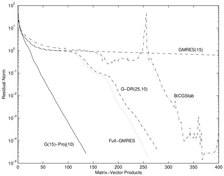
Figure 1: Solution of second right-hand side.

For the first right-hand side, BiCGStab uses more matrix-vector products than GMRES-DR but considerably less flops. BiCGStab needs 17.5 million flops versus 81.1 million for GMRES-DR to improve the residual norm by $10^{-6}$. However, GMRES-Proj saves on both matrix-vector products and flops for the second right-hand side. It uses 130 matrix-vector products compared to 365 for BiCGStab and 14.1 million flops versus 17.5. Of course GMRES-Proj needs GMRES-DR applied first, but if there are a number of right-hand sides, the GMRES approach can still be competitive in terms of flops even for such a very sparse matrix. For example, if there are 10 right-hand sides, then GMRES-DR for the first right-hand side and GMRES-Proj for the next nine takes 1405 matrix-vector products and 204.5 million flops. BiCGStab on all 10 right-hand sides uses 4113 matrix-vector products and 197.6 million flops.

III.2 Effect in GMRES-Proj of the size of the GMRES subspace

We experiment with changing the size of the GMRES subspaces used to solve the subsequent right-hand sides. The same problem from the experiment in the previous subsection is considered with again the first right-hand side solved with GMRES-DR(25,10). This time ten right-hand sides are solved, with different $m$ values for GMRES(m)-Proj(10). The first column of Table 1 gives the total number of matrix-vector products required to solve all ten systems. We see that even with deflation, larger subspaces are helpful. However, if the matrix-vector product is inexpensive, using a small value of $m$ such as $m=10$ might be more efficient than $m=20$ in spite of increased iterations.

Table 1: Changing $m$ and the frequency of projection for GMRES-Proj

	project every cycle	project every 5th	project every 10th	project at 10,20, …
$m$	mat-vec’s	mat-vec’s	mat-vec’s	mat-vec’s
5	2440	2577	2596	1962
10	1658	1678	1636	1604
15	1405	1411	1673	1910
20	1298	1330	2107	2438
25	1257	1478	2521	2843

III.3 Projecting less frequently

Table 1 also shows the effect of not projecting between every cycle of GMRES(m). For small values of $m$, it is not necessary to project very often. Projecting reduces components of $r$ in the directions of the eigenvectors corresponding to small eigenvalues, and these components may not need to be reduced futher for a while (basically until the rest of the residual vector has been reduced to the point that these components are again significant). For $m=10$, projecting every tenth cycle is good enough. For $m=20$, projecting every fifth is almost as good as projecting every cycle, while projecting every tenth is not as effective.

In the case of $m=5$ and project every tenth cycle, the projections

are performed before the 1st, 11th, 21st, …cycles of GMRES. If instead we project before the 10th, 20th, …cycles, the results are better, with only 1962 matrix-vector products needed instead of 2596 (see the last column of Table 1). It is not clear why the convergence is better if no projection is performed until after nine cycles of GMRES.

III.4 Solving the first right-hand side to greater accuracy

We test here the notion that the eigenvector approximations provided by GMRES-DR might not be optimal at the same point that the linear equations are considered solved. For the case of Example 1, solving 10 right-hand sides with $rtol$ of $10^{-6}$ requires 1405 iterations. But if the system with the first right-hand side is solved to greater accuracy of $10^{-8}$, while the final nine systems are again are solved to $10^{-6}$, the total number of iterations drops to 1343. This is in spite of the fact that solution of the first system takes 69 more iterations. The average savings per subsequent right-hand side is 13.6 iterations. However, solving the first right-hand side to even greater accuracy does not pay off. With relative tolerance of $10^{-10}$, 1388 iterations are needed for all ten right-hand sides (exempting the first, the number actually stays the same as for the first $rtol$ being $10^{-8}$).

III.5 Comparison with other deflation approaches

While the GMRES-Proj method deflates eigenvalues with a projection that is separate from the GMRES phase, there are other ways of deflating eigenvalues as discussed at the beginning of this section. We will compare GMRES-Proj with the versions of GMRES-E and DEFLATION that use eigenvectors to augment or precondition, but are adapted so they do not attempt to improve on the eigenvectors. Note GMRES-DR is used on the first right-hand side to compute the eigenvectors for each method, then nine additional right-hand sides are solved. We see from the results in Table 2 that the methods perform similarly. However, as mentioned earlier, there is a difference in expense, since GMRES-Proj uses eigenvectors only once per cycle. DEFLATION applies eigenvectors at every iteration, and the cost above the normal GMRES expense is $2k$ length $n$ vector operations per iteration or about $2km$ per cycle. Costs for GMRES-E with $k$ approximate eigenvectors augmenting a $m$-dimensional Krylov subspace are a little greater than for DEFLATION (extra expense of about $2km+k^{2}$ length $n$ vector operations per cycle). Meanwhile, as mentioned, GMRES-Proj requires about $3k$ extra per cycle. So GMRES-Proj can be more efficient. However, for very expensive matrix-vector product or for small $k$, GMRES-Proj may not be a significantly better way of deflating.

Table 2: Comparson of different deflation approaches

	eigenvectors used for projection:	eigenvectors in subspace:	eigenvector preconditioner:
$m$	GMRES-Proj	GMRES-E	DEFLATION
5	2440	2565	2528
10	1658	1658	1613
15	1405	1405	1387
20	1298	1296	1284
25	1257	1251	1241

III.6 Comparison with block-QMR

Here we show that the GMRES-Proj method can be competitive with block methods. Specifically, we compare against block-QMR [26] for 10 right-hand sides. GMRES(15)-Proj(10) uses projections every fifth GMRES cycle. Table 3 has the results for both the number of matrix-vector products and the number of flops as counted by MATLAB. GMRES-Proj is a little better than block-QMR in terms of flops, since block-QMR with blocksize 10 has significant orthogonalization expense. (Table 4 includes comparison with 40 right-hand sides.)

Table 3: Comparison with nonrestarted methods including block QMR

Method	matrix-vector products	Mflops
GMRES-DR + GMRES-Proj	1411	198.3
Block-QMR	1782	567.5
QMR, 10 times	5220	245.7
BiCGStab, 10 times	4113	197.6

III.7 The case of related right-hand sides

One expects intuitively that if the right-hand sides are closely related to each other then there should be a way to take advantage of the situation. However, it is discussed in [27] that block methods may not be successful at this. We suggest here a simple way for GMRES-Proj to deal with this case. For the second and subsequent right-hand sides, projections are done over all previously computed solutions (step 2 of the GMRES-Proj algorithm). We project over each solution vector individually, but another option is to project over all at once.

We again compare GMRES-Proj with block-QMR for 10 right-hand sides. This time the first has random normal entries and all the others are equal to the first one plus $10^{-4}$ times a random vector. GMRES-Proj is better able to take advantage of the related right-hand sides, because it solves them sequentially, and the results of one solution are available for the next problem. GMRES-Proj uses only 521 matrix-vector products compared to 1702 for block-QMR. In terms of flops, GMRES-Proj needs 110 million versus to 542 million for block-QMR.

III.8 A QCD Example

We demonstrate the GMRES-Proj method for an application from particle physics. In lattice quantum chromodynamics (QCD), very large systems of linear equations arise that have complex non-Hermitian matrices. For such matrices, we need to change transpose to Hermitian transpose in the algorithms. Often there are multiple right-hand sides for each QCD matrix. However, block methods are not typically used. The matrix-vector product is moderately expensive (it can be implemented for a cost equivalent to 72 non-zeros per row [28] even though there would actually be about three times as many non-zeros in the matrix if it was formed). The orthogonalization costs are significant enough to discourage block methods. Therefore it would be very useful to improve convergence of the main methods used for QCD problems such as restarted GMRES and BiCGStab. Our application of deflation to multiple right-hand sides is new; however, deflation in the context of lattice problems was originally considered in [29]. See [31, 30, 32] for other approaches.

Example 2.

We look at a typical Wilson-Dirac matrix from QCD. It has even-odd preconditioning [25], and the dimension is 248,832 by 248,832. The value of $\kappa$ is 0.159, which is approximately $\kappa_{critical}$, so the leftmost eigenvalues are near the imaginary axis. The right-hand sides are unit vectors associated with particular space-time, Dirac and color coordinates. The first right-hand side is solved with GMRES-DR(50,30) to three different residual tolerances. Then for the second right-hand side, GMRES-Proj uses 30 approximate eigenvectors for the projection in between cycles of GMRES(20). See Figure 2 for the results. Solving the first right-hand side to one of the more demanding tolerances ($10^{-10}$ or $10^{-14}$) pays off. GMRES(20)-Proj(30) can converge in less than one-tenth of the iterations needed for GMRES(20).

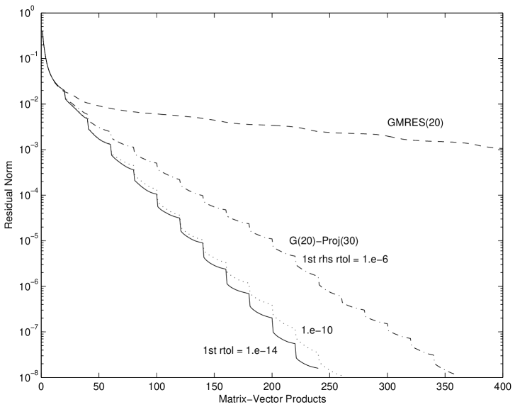
Figure 2: Solution of second RHS for large QCD matrix.

Figure 3 shows convergence with different frequencies of projection for GMRES(20)-Proj(30) with the first right-hand side solved to $rtol=10^{-10}$ . Projecting in between every cycle turns out a little better (for a different QCD matrix in [25], projecting every third cycle was as effective as every cycle).

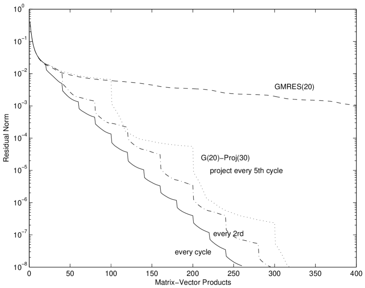
Figure 3: Different frequencies of projection for the QCD matrix.

Figure 4 shows the harmonic Ritz values generated by GMRES-DR(50,30) after 50, 550 and 890 matrix-vector products. The case of 550 corresponds to $rtol=10^{-10}$. Figure 5 has a blowup of the portion of that graph near the origin. After 550 iterations, the small approximate eigenvalues are settling in near to where they are after 890. These graphs show why deflating eigenvalues is so effective for this problem. The origin is halfway surrounded by eigenvalues, until the smallest ones are deflated.

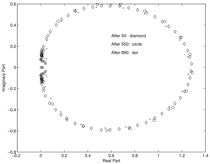
Figure 4: Harmonic Ritz values from GMRES-DR with the QCD matrix.

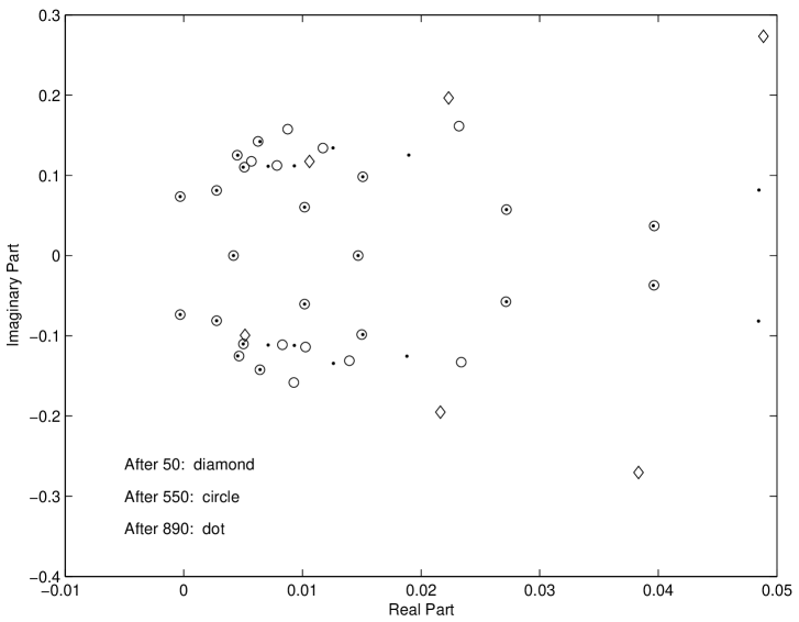
Figure 5: Closeup of harmonic Ritz values near the origin.

IV Deflation for Nonrestarted Methods

IV.1 A simple deflated BiCGSTAB

Nonrestarted methods are popular, because they use a large Krylov subspace but don’t have excessive expense or storage. For difficult problems, nonrestarted methods often converge much faster than regular restarted GMRES. Deflated versions of GMRES are usually more competitive, but there are still problems for which nonrestarted methods are preferable. This is particularly true for the case of fairly inexpensive matrix-vector product, or when storage is limited. We now look at using deflation to improve BiCGSTAB and other nonrestarted methods for multiple right-hand sides. As in the previous section, we plan to apply GMRES-DR to the first right-hand side and then use the eigenvector information generated to assist with the other right-hand sides. However, a projection is only possible at a restart. Therefore a nonrestarted iterative method must rely on just one projection, before the iteration begins. We note that deflation could be applied during the iteration with an eigenvector preconditioner [5] and possibly similar to [33], where eigenvectors are worked into the conjugate gradient algorithm. However, here we only consider using a projection over the subspace of approximate eigenvectors. A deflated version of BiCGStab that can be applied to the second and subsequent right-hand sides is now given. It will later be modified.

Preliminary BiCGStab-Proj(k)

1. After applying the initial guess $x_{0}^{(i)}$, let the system

   of equations be $A(x^{(i)}-x_{0}^{(i)})=r_{0}^{(i)}$.

2. Apply the minres projection using the $V_{k+1}$ and $\bar{H}_{k}$ matrices developed while solving the first right-hand side with GMRES-DR.

3. Apply BiCGStab until satisfied with convergence.

Example 3. We use the same matrix and right-hand sides as in Example 1. The first right-hand side is solved using GMRES-DR with $rtol=10^{-8}$. Ten eigenvectors are calculated with GMRES-DR(25,10) and five with GMRES-DR(25,5). Figure 6 shows the effect of projecting before BiCGSTAB. With projection of 10 eigenvectors, the method is effective. With five eigenvectors, the projection actually makes things worse. The good effect appears to wear off. This is because the components of the residual vector in the directions of the the eigenvectors corresponding to the smallest eigenvalues are not reduced enough by the projection. The BiCGStab iteration must eventually confront the small eigencomponents. Partially removing these components can make it more difficult for BiCGStab to develop these eigenvectors, since then BiCGStab has a poor starting vector for that task. So partially removing eigencomponents can slow down eventual convergence.

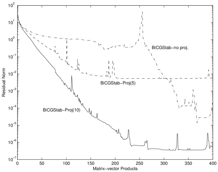
Figure 6: Deflation for BiCGStab using only right eigenvectors.

The minres projection simply does not do a good job. Even though in some sense it is the best projection, it does not necessarily reduce small eigencomponents enough. To see the problem with the minres projection, we assume that we have one exact real eigenvector. We would like to be able to eliminate the component of the residual vector in that direction, but the minres projection does not necessarily accomplish this.

THEOREM 4.1. Suppose $A$ has a full set of eigenvectors. Let $z_{1},z_{2},\ldots,z_{n}$ be the normalized eigenvectors. Let the current linear equations problem be $A(x-x_{0})=r_{0}$, with $r_{0}=\alpha_{1}z_{1}+\alpha_{2}z_{2}+\ldots+\alpha_{n}z_{n}$. Then after the minres projection over the subspace $Span\{z_{1}\}$, the new residual’s component in the direction of $z_{1}$ is

$$-\sum_{i=2}^{n}\alpha_{i}z_{1}^{T}z_{i}.$$ (3)

Proof. Let $V$ be an othonormal matrix with columns spanning the desired subspace (the columns may be complex). The minres projection is equivalent [24] to solving

$$V^{T}A^{T}AVd=V^{T}A^{T}r_{0}$$ (4)

for $d$. The new residual vector is then $r=r_{0}-AVd$.

With projection over one exact eigenvector $z_{1}$, Equation (4) becomes

$$z_{1}^{T}A^{T}Az_{1}d=z_{1}^{T}A^{T}r_{0},$$

which gives

$$\lambda_{1}^{2}d=\lambda_{1}\sum_{i=1}^{n}\alpha_{i}z_{1}^{T}z_{i}.$$

Then after solving for $d$, and with $r=r_{0}-d\lambda_{1}z_{1}$, the $z_{1}$ component of $r$ is as given in Equation (3).

Equation 3 shows that the minres projection over one exact eigenvector works best if the components of the residual in the directions other than $z_{1}$ are small and if the eigenvectors are nearly orthogonal. For nonsymmetric matrices, this projection may only reduce the size of the $z_{1}$ component to roughly the size of the other components. There is no reason to expect the $z_{1}$ component to be reduced far enough so that it will not need any further reduction from the BiCGStab iteration.

IV.2 Restarting deflated BiCGSTAB

One way to remedy the imperfection of the minres projection is to do another projection along the way to further reduce the size of the components of the residual vector in the directions of the smallest eigenvectors. However, this requires a restart.

Example 4.

Figure 7 shows what happens if deflated BiCGSTAB using five eigenvectors is restarted once with an additional projection at the restart. Three different runs are shown, with the restarts at 100, 150 and 200 matrix-vector products. This approach seems fairly effective, although the restart at 100 is too early and the residual norm plateaus around $10^{-4}$. There may be cases where an occasionally restarted version of deflated BiCGSTAB is useful. The restarting would generally not need to be as frequent as for deflated GMRES, because there are no growing orthogonalization costs for BiCGSTAB. However, the idea of restarting a normally nonrestarted method such as BiCGSTAB is not appealing and might slow down convergence for difficult problems. Also, it may be difficult to know the appropriate point or points at which to restart. We will next look at another possible approach that avoids restarting but needs left eigenvectors.

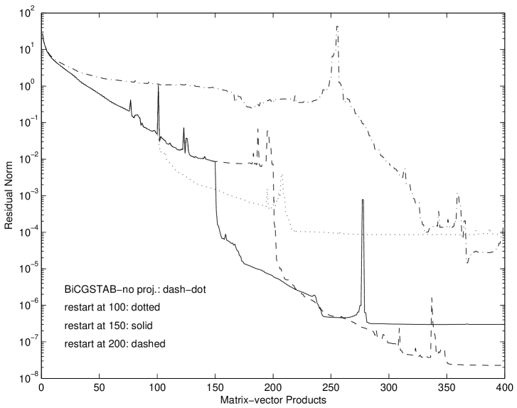
Figure 7: Restarting deflated BiCGSTAB at different points.

IV.3 A projection with left and right eigenvectors

We give a projection over both left and right eigenvectors that does a much better job of reducing the eigencomponents of the residual in the directions of already determined eigenvectors. It is simply a Petrov-Galerkin projection [24] with the right space spanned by approximate right eigenvectors and the left space spanned by approximate left eigenvectors.

Left-right Projection

1. Let the current approximate solution be $x_{0}$ and the current system of equations be $A(x-x_{0})=r_{0}$. Let $V$ have columns spanned by approximate right eigenvectors and let the columns of $W$ be spanned by approximate left eigenvectors (we choose both $V$ and $W$ to be orthonormal).

2. Solve $W^{T}AVd=W^{T}r_{0}$.

3. The new approximate solution is $x_{k}=x_{0}+Vd$.

4. The new residual vector is $r_{k}=r_{0}-AVd$.

THEOREM 4.2. Suppose $A$ has a full set of eigenvectors. Let $z_{1},z_{2},\ldots,z_{n}$ be the right eigenvectors of length one and $u_{1},u_{2},\ldots,u_{n}$ be the left eigenvectors normalized so that $u_{i}^{T}z_{i}=1$. Let the current linear equations problem be $A(x-x_{0})=r_{0}$, with $r_{0}=\alpha_{1}z_{1}+\alpha_{2}z_{2}+\ldots+\alpha_{n}z_{n}$. Then after the left-right projection with right subspace $Span\{z_{1}\}$ and left subspace $Span\{w\}$, where $w=\sum_{i=1}^{n}\beta_{i}u_{i}$, the new residual’s component in the direction of $z_{1}$ is

$$-\sum_{i=2}^{n}\alpha_{i}{\beta_{i}\over\beta_{1}}.$$ (5)

Proof. Putting $V=z_{1}$ and $W=w$ into $W^{T}AVd=W^{T}r_{0}$, we get

$$w^{T}Az_{1}d=w^{T}r_{0},$$

which using the biorthogonality of the left and right eigenvectors gives

$$\lambda_{1}\beta_{1}d=\sum_{i=1}^{n}\alpha_{i}\beta_{i}.$$

Then $d={\alpha_{1}\over\lambda_{1}}+{1\over\lambda_{1}}\sum_{i=2}^{n}\alpha_{i}{\beta_{i}\over\beta_{1}}$, and with $r=r_{0}-d\lambda_{1}z_{1}$, the $z_{1}$ component of $r$ is as given in Equation (5).

This theorem tells us that the left-right projection does a better job of reducing the size of the residual’s component in the $z_{1}$ direction if the other components are small and if the left vector $w$ is mostly in the direction of the left eigenvector $u_{1}$. If $w=u_{1}$, then the component in the direction of $z_{1}$ is zeroed out. This holds true even for projections over more than one vector.

THEOREM 4.3. Suppose $A$ has a full set of eigenvectors. Then with a Petrov-Galerkin projection with $z_{1}$ contained in the right subspace and the corresponding left eigenvector $u_{1}$ in the left subspace, the component of the residual in the direction of $z_{1}$ is zeroed out.

Proof. Let the current linear equations problem be $A(x-x_{0})=r_{0}$, with $r_{0}=\alpha_{1}z_{1}+\alpha_{2}z_{2}+\ldots+\alpha_{n}z_{n}$.

Let $Z$ and $U$ be matrices with right and left eigenvectors respectively as columns, ordered so that the desired eigenvector is first and normalized so that $U^{H}Z=I$.

For the projection, without loss of generality $W$ can be chosen to have first column equal to ${u_{1}\over||u_{1}||}.$ Let $k$ be the number of columns in $W$. Then $W=UB$, with $B$ an $n$ by $k$ matrix with first column equal to $[{1\over||u_{1}||},0,0,\ldots 0]^{T}$. Also using $A=Z\Lambda U^{H}$, the problem $W^{T}AVd=W^{T}r_{0}$ can be written as

$$B^{H}U^{H}Z\Lambda U^{H}Vd=W^{T}r_{0}.$$

Since $\hat{x}=Vd$, this becomes

$$B^{H}\Lambda U^{H}\hat{x}=W^{T}r_{0}.$$

Now $W^{T}r_{0}$ has first entry ${\alpha_{1}\over||u_{1}||}$. Using the forms of $B$ and $\Lambda$, we see the solution is such that $U^{H}\hat{x}$ has first entry equal to ${\alpha_{1}\over\lambda_{1}}$, and that is the component of $\hat{x}$ in the direction of $z_{1}$. The component of $A\hat{x}$ in the direction of $z_{1}$ is then just $\alpha_{1}$. So the component of $r=r_{0}-A\hat{x}$ in that direction is zero.

Example 5. We use the same matrix and right-hand sides as in Example 1. The first right-hand side is solved using GMRES-DR with $rtol=10^{-8}$. Ten eigenvectors are calculated with GMRES-DR(25,10) and five with GMRES-DR(25,5). The left eigenvectors were computed separately using the same algorithms applied to the transpose of $A$. Figure 8 shows the effect of using the left-right projection before BiCGSTAB. Projecting with either five or 10 right and left approximate eigenvectors improves the result considerably over non-deflated BiCGSTAB and also improves compared to just projecting with right eigenvectors. We also compute the left eigenvectors to greater accuracy (using 20 cycles of GMRES(40,20) applied to $A^{T}$, then taking the eigenvectors corresponding to the smallest five or 10 eigenvalues), and the results are even better. On the graph these results are noted as “accurate left”. As suggested by Theorem 4.2, the accuracy of the left eigenvectors in the projection is important.

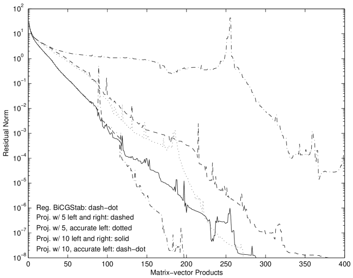
Figure 8: Deflation for BiCGStab using right and left eigenvectors.

IV.4 The special case of QCD matrices

For the Wilson-Dirac matrix from lattice QCD, there is a relationship between the right and left eigenvectors that can be exploited. Using that a certain matrix $\gamma_{5}$ [28, 34] symmetrizes the matrix $A$, it can be shown that the left eigenvector corresponding to an eigenvalue is $\gamma_{5}$ times the right eigenvector corresponding to the complex conjugate of the eigenvalue. So if we calculate the right eigenvectors for the smallest eigenvalues (including both of any complex conjugate pairs), then $\gamma_{5}$ times this set gives the left eigenvectors. Because of the simple form for $\gamma_{5}$, there is no additional cost for the left eigenvectors. We next give an example showing that deflating eigenvalues from BiCGStab can be helpful in QCD.

Example 6.

We use a small QCD matrix. It is complex with dimension 1536. Solution of the second right-hand side has a left-right projection to deflate either eight or 16 eigenvalues followed by BiCGStab. The right eigenvectors are from solution of the first right-hand side with GMRES-DR and the left eigenvectors come from the relationship with the right eigenvectors. Figure 9 shows that to reach residual norm of $10^{-6}$ requires only about one-third as many iterations of deflated BiCGStab as plain BiCGStab if 16 approximate eigenvectors are projected.

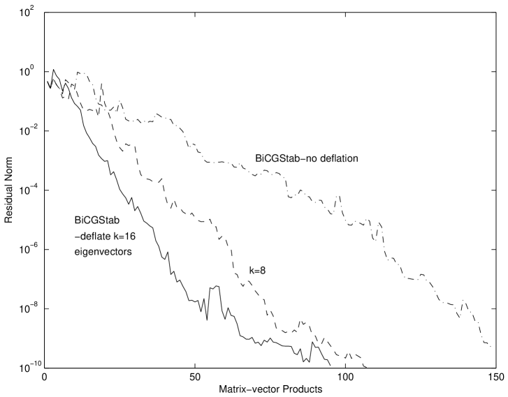
Figure 9: Deflated BiCGStab for a small QCD example.

V Block Methods

Block methods are well-known for solving systems of equations with multiple right-hand sides. We saw in Subsection III.F an example for which GMRES-Proj is better than block-QMR in terms of both matrix-vector products and flops. However, with more right-hand sides in the next example, block-QMR is best in terms of matrix-vector products. So there are situations with expensive matrix-vector product where block methods are needed. This is particularly the case when the matrix-vector product can be efficiently applied to several right-hand sides simultaneously. In this section we look at combining GMRES-Proj with block methods.

A block GMRES method with deflated restarting called block-GMRES-DR is proposed in [27]. Here we look at the situation where a block method is worth considering, but there are more right-hand sides than can be efficiently solved with a single block run. This could be either because the orthogonalization expense or storage would be too great or because not all right-hand sides are available at once. We propose to solve the first group of say $p$ right-hand sides with block-GMRES-DR(m,p,k) (subspaces of dimension $m$ are used, the block-size is $p$, and $k$ approximate eigenvectors are generated). The eigenvectors satisfy a block Arnoldi-like recurrence of the form $AV_{k}=V_{k+p}\bar{H}_{m}$, where $V_{k}$ is an orthonormal matrix with columns spanning the space of approximate eigenvectors, $V_{k+p}$ has $p$ columns appended to $V_{k}$, and $\bar{H}_{k}$ is $k+p$ by $k$. For the next group of $p$ right-hand sides, we alternate minres projections over the approximate eigenvectors with cycles of block-GMRES. Other right-hand sides are dealt with the same way, $p$ at a time.

Bl-GMRES(m,p)-Proj(k)

1. Apply initial guesses to the current $p$ right-hand sides being considered.

2. Apply the Minres Projection to all $p$ systems using the $V_{k+p}$ and $\bar{H}_{k}$ matrices developed while solving the first $p$ right-hand sides with Bl-GMRES-DR(m,p,k).

3. Apply one cycle of Bl-GMRES(m,p).

4. Test the residual norms for convergence (can also test during the Bl-GMRES cycles). If not satisfied, go back to step 2.

Example 7. We test the matrix of Example 1 for 40 right-hand sides. See Table 4 for the results. The method Bl-G-DR(170,20,10) + Bl-G(160,20)-Proj(10) means that Block-GMRES-DR with block-size of 20, 10 approximate eigenvectors, and total subspaces of dimension 170 is applied to the first 20 right-hand sides. Then for the next 20 right-hand sides, minres projection over the 10 approximate eigenvectors is alternated with Block-GMRES using block-size of 20 and subspaces of maximum dimension 160. However, for this problem Block-GMRES-DR does not converge. The dimension of the Krylov subspace generated for each right-hand side is just 8, which is not enough for this difficult problem. With block-size of 5, the method Bl-G-DR(170,5,10) + Bl-G(160,5)-Proj(10) uses many more flops than the non-block GMRES-Proj approach, but it does use less matrix-vector products. Block-QMR uses even fewer matrix-vector products, and it can potentially take advantage of applying 40 matrix-vector products simultaneously. Block-QMR builds a very large subspace that eventually contains approximations to many eigenvectors, thus giving this rapid convergence. If one is only interested exclusively in the number of matrix-vector products, Bl-GMRES-DR can actually be the winner. Only 2400 matrix-vector products are needed for Bl-GMRES-DR(1220,40,20).

Table 4: Comparison of block-GMRES-Proj with other methods for 40 right-hand sides

Method	matrix-vector products	Mflops
GMRES-DR(25,10) + GMRES(15)-Proj(10)	5151	6.1
Bl-G-DR(170,20,10) + Bl-G(160,20)-Proj(10)	-	-
Bl-G-DR(170,10,10) + Bl-G(160,10)-Proj(10)	4960	170.4
Bl-G-DR(170,5,10) + Bl-G(160,5)-Proj(10)	4169	116.6
Bl-G-DR(60,5,10) + Bl-G(50,5)-Proj(10)	5900	30.9
Bl-QMR	3298	117.2

V.1 Deflating Block-QMR

Deflation can be used to help block-QMR, as in the section on deflated BiCGStab. We can use both left and right eigenvectors to remove small eigenvalue components then apply the block method. While improving block-QMR is an interesting idea, it is not so easy to do.

We continue the experiments in Example 7. We use 10 right and left eigenvectors (with the accurate left eigenvectors from Example 5) to deflate, then apply block-QMR. Table 5 has the number of matrix-vector products that are required. With three right-hand sides, the number of matrix-vector products is reduced significantly, from 922 to 538. We also tried using 20 right and left eigenvectors and the number of matrix-vector products went down to 412. However, the improvement is not so good for larger blocks. Regular block-QMR manages its own deflation of eigenvalues as it builds large subspaces.

Deflated block-QMR does converge quicker at the initial stages. For instance, if the convergence tolerance is only $10^{-4}$ for 10 right-hand sides, then the deflated approach reduces the number of matrix-vector products by 31% (from 1570 to 1076) compared to 22% (from 1782 to 1384) for tolerance of $10^{-6}$.

Table 5: Test of deflated block-QMR

number of right-hand sides	Bl-QMR	deflated Bl-QMR
1	534	180
3	922	538
5	1256	838
10	1782	1384
20	2452	2116
40	3298	3074

VI Conclusion

In this paper, we have shown that deflating eigenvalues can be very helpful for solving systems with multiple right-hand sides. The first right-hand side is solved with the deflated GMRES method GMRES-DR. This method develops eigenvector information that is used for all subsequent right-hand sides. Therefore there is no requirement that the right-hand sides all be available simultaneously. Also, since the needed eigenvector information is available from the beginning for the subsequent right-hand sides, the convergence can be much faster, particularly for tough problems with small eigenvalues. The approach in GMRES-Proj of projecting in between cycles of GMRES is very efficient. For the case of related right-hand sides, there is a simple, but especially effective approach.

In lattice QCD physics, very large systems with multiple right-hand sides need to be solved. In one example, GMRES-Proj is an order of magnitude better that regular restarted GMRES.

Block methods are a competing approach. However, block methods can be combined with deflation of eigenvalues by not solving all systems at once.

For non-restarted methods such as BiCGStab, deflating eigenvalues can also be useful. Approximate eigenvectors from solving the first right-hand side with GMRES-DR can be projected one time, but both right and left eigenvectors are needed. For many QCD matrices, left eigenvectors are available once the right eigenvectors have been computed. Since BiCGStab is a popular method in QCD, this new approach should be useful.

Future research will focus on deflating eigenvalues for QCD problems which not only have multiple right-hand sides, but have multiple shifts of the matrix for each right-hand side. The goal is to solve all the shifted systems for approximately the same cost as solving one. It would also be worthwhile to investigate deflation for other QCD problems such as twisted mass and overlap fermions.

For problems that are not from QCD, the need for both left and right eigenvectors for deflated BiCGStab makes development of a deflated restarted BiCG or QMR method desirable. This method would solve linear equations and simultaneously compute left and right eigenvectors.

References

- [1] V. Simoncini and E. Gallopoulos. An iterative method for nonsymmetric systems with multiple right-hand sides. SIAM J. Sci. Comput., 16:917–933, 1995.
- [2] Y. Saad and M. H. Schultz. GMRES: a generalized minimum residual algorithm for solving nonsymmetric linear systems. SIAM J. Sci. Statist. Comput., 7:856–869, 1986.
- [3] H. A. van der Vorst. Bi-CGSTAB: A fast and smoothly converging variant of Bi-CG for the solution of non-symmetric linear systems. SIAM J. Sci. Statist. Comput., 12:631–644, 1992.
- [4] J. Baglama, D. Calvetti, G. H. Golub, and L. Reichel. Adaptively preconditioned GMRES algorithms. SIAM J. Sci. Comput., 20:243–269, 1998.
- [5] K. Burrage and J. Erhel. On the performance of various adaptive preconditioned GMRES strategies. Num. Lin. Alg. with Appl., 5:101–121, 1998.
- [6] C. Le Calvez and B. Molina. Implicitly restarted and deflated GMRES. Numer. Algo., 21:261–285, 1999.
- [7] A. Chapman and Y. Saad. Deflated and augmented Krylov subspace techniques. Num. Lin. Alg. with Appl., 4:43–66, 1997.
- [8] E. De Sturler. Truncation strategies for optimal Krylov subspace methods. SIAM J. Numer. Anal., 36:864–889, 1999.
- [9] J. Erhel, K. Burrage, and B. Pohl. Restarted GMRES preconditioned by deflation. J. Comput. Appl. Math., 69:303–318, 1996.
- [10] S. A. Kharchenko and A. Y. Yeremin. Eigenvalue translation based preconditioners for the GMRES(k) method. Num. Lin. Alg. with Appl., 2:51–77, 1995.
- [11] R. B. Morgan. A Restarted GMRES Method Augmented with Eigenvectors. SIAM J. Matrix Anal. Appl., 16:1154–1171, 1995.
- [12] R. B. Morgan. Implicitly Restarted GMRES and Arnoldi Methods for Nonsymmetric Systems of Equations. SIAM J. Matrix Anal. Appl., 21:1112–1135, 2000.
- [13] R. B. Morgan. GMRES with Deflated Restarting. SIAM J. Sci. Comput., 24:20–37, 2002.
- [14] Y. Saad. Analysis of augmented Krylov subspace techniques. SIAM J. Matrix Anal. Appl., 18:435–449, 1997.
- [15] D. C. Sorensen. Implicit application of polynomial filters in a k-step Arnoldi method. SIAM J. Matrix Anal. Appl., 13:357–385, 1992.
- [16] K. Wu and H. Simon. Thick-restart Lanczos method for symmetric eigenvalue problems. SIAM J. Matrix Anal. Appl., 22:602 – 616, 2000.
- [17] R. B. Morgan. On restarting the Arnoldi method for large nonsymmetric eigenvalue problems. Math. Comp., 65:1213–1230, 1996.
- [18] G. W. Stewart. A Krylov–Schur algorithm for large eigenproblems. SIAM J. Matrix Anal. Appl., 23:601 – 614, 2001.
- [19] R. B. Morgan and M. Zeng. Harmonic Restarted Arnoldi for Calculating Eigenvalues and Determining Multiplicity. Preprint, 2003.
- [20] R. B. Morgan. Computing interior eigenvalues of large matrices. Linear Algebra Appl., 154-156:289–309, 1991.
- [21] R. W. Freund. Quasi-kernel polynomials and their use in non-Hermitian matrix iterations. J. Comput. Appl. Math., 43:135–158, 1992.
- [22] C. C. Paige, B. N. Parlett, and H. A. van der Vorst. Approximate solutions and eigenvalue bounds from Krylov subspaces. Num. Lin. Alg. with Appl., 2:115–133, 1995.
- [23] R. B. Morgan and M. Zeng. Harmonic projection methods for large non-symmetric eigenvalue problems. Num. Lin. Alg. with Appl., 5:33–55, 1998.
- [24] Y. Saad. Iterative Methods for Sparse Linear Systems. PWS Publishing, Boston, MA, 1996.
- [25] R. B. Morgan and W. Wilcox. Deflation of Eigenvalues for GMRES in Lattice QCD. Nucl. Phys. B (Proc. Suppl.), 106:1067–1069, 2002.
- [26] R. W. Freund and M. Malhotra. A block QMR algorithm for non-Hermitian linear systems with multiple right-hand sides. Linear Algebra Appl., 254:119–157, 1997.
- [27] R. B. Morgan. Restarted block GMRES with deflation of eigenvalues. 2003.
- [28] A. Frommer and B. Medeke. Exploiting structure in Krylov subspace methods for the Wilson fermion matrix. Technical Report BUGHW-SC 97/3, Bergische Universität Wüppertal, Wüppertal, Germany, 1997.
- [29] P. de Forcrand. Progress on Lattice QCD Algoriths. Nucl. Phys. B (Proc. Suppl.), 47:228–235, 1996.
- [30] S. J. Dong, F. X. Lee, K. F. Liu, and J. B. Zhang. Chiral symmetry, quark mass, and scaling of the overlap fermions. Phys. Rev. Lett., 85:5051–5054, 2000.
- [31] R. G. Edwards, U. M. Heller, and R. Narayanan. Study of Chiral Symmetry in Quenched QCD Using the Overlap Dirac Operator. Phys. Rev. D, 59:0945101–0945108, 1999.
- [32] H. Neff, N. Eicker, Th. Lippert, J. W. Negele, and K. Schilling. On the low fermionic eigenmode dominance in QCD on the lattice. Preprint, hep-lat/0106016., 2001.
- [33] Y. Saad, M. C. Yeung, J. Erhel, and F. Guyomarc’h. A deflated version of the conjugate gradient algorithm. SIAM J. Sci. Comput., 21:1909–1926, 2000.
- [34] A. Frommer. Linear Systems Solvers - Recent Developments and Implications for Lattice Computations. Nucl. Phys. B (Proc. Suppl.), 53:120–126, 1997.