Height fluctuations in the honeycomb dimer model

Abstract

We study a model of random surfaces arising in the dimer model on the honeycomb lattice. For a fixed “wire frame” boundary condition, as the lattice spacing $\epsilon\to 0$, Cohn, Kenyon and Propp [3] showed the almost sure convergence of a random surface to a non-random limit shape $\Sigma_{0}$. In [11], Okounkov and the author showed how to parametrize the limit shapes in terms of analytic functions, in particular constructing a natural conformal structure on them. We show here that when $\Sigma_{0}$ has no facets, for a family of boundary conditions approximating the wire frame, the large-scale surface fluctuations (height fluctuations) about $\Sigma_{0}$ converge as $\epsilon\to 0$ to a Gaussian free field for the above conformal structure. We also show that the local statistics of the fluctuations near a given point $x$ are, as conjectured in [3], given by the unique ergodic Gibbs measure (on plane configurations) whose slope is the slope of the tangent plane of $\Sigma_{0}$ at $x$.

1 Introduction

1.1 Dimers and surfaces

A dimer covering, or perfect matching, of a finite graph is a set of edges covering all the vertices exactly once. The dimer model is the study of random dimer coverings of a graph. Here we shall for the most part deal with the uniform measure on dimer coverings.

In this paper we study the dimer model on the honeycomb lattice (the periodic planar graph whose faces are regular hexagons), or rather, on large pieces of it. This model, and more generally dimer models on other periodic bipartite planar graphs, are statistical mechanical models for discrete random interfaces. Part of their interest lies in the conformal invariance properties of their scaling limits [8, 9].

Dimer coverings of the honeycomb graph are dual to tilings with $60^{\circ}$ rhombi, also known as lozenges, see Figure 1.

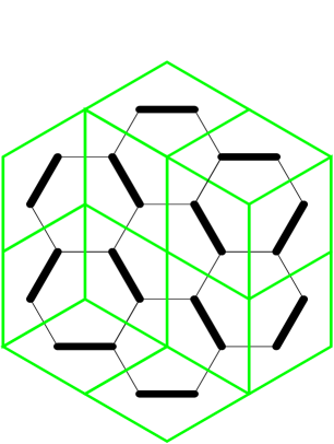
Figure 1: Honeycomb dimers (solid) and the corresponding “lozenge” tiling (green).

Lozenge tilings can in turn be viewed as orthogonal projections onto the plane $P_{111}=\{x+y+z=0\}$ of stepped surfaces which are polygonal surfaces in ${\mathbb{R}}^{3}$ whose faces are squares in the $2$-skeleton of ${\mathbb{Z}}^{3}$ (the stepped surfaces are monotone in the sense that the projection is injective), see Figures 1,3. Each stepped surface is the graph of a function, the normalized height function, on the underlying tiling, which is linear on each tile. This function is defined simply as $\sqrt{3}$ times the distance from the surface to the plane $P_{111}$. (The scaling factor $\sqrt{3}$ is just to make the function integer-valued on ${\mathbb{Z}}^{3}$.)

1.2 Results

We are interested in studying the scaling limit of the honeycomb dimer model, that is, the limiting behavior of a uniform random dimer covering of a fixed plane region $U$ when the lattice spacing $\epsilon$ goes to zero. Equivalently, we take stepped surfaces in $\epsilon{\mathbb{Z}}^{3}$ and let $\epsilon\to 0$. As boundary conditions we are interested in stepped surfaces spanning a “wire frame” which is a simple closed polygonal path $\gamma_{\epsilon}$ in $\epsilon{\mathbb{Z}}^{3}$. We take $\gamma_{\epsilon}$ converging as $\epsilon\to 0$ to a smooth path $\gamma$ which projects to $\partial U$.

1.2.1 Limit shape

Let $U$ be a domain in $P_{111}$, and $\gamma$ be a smooth closed curve in ${\mathbb{R}}^{3}$, projecting orthogonally to $\partial U$. For each $\epsilon>0$ let $\gamma_{\epsilon}$ be a nearest-neighbor path in $\epsilon{\mathbb{Z}}^{3}$ approximating $\gamma$ (in the Hausdorff metric) and which can be spanned by a monotone stepped surface $\Sigma_{\epsilon}$, monotone in the sense that it projects injectively to $P_{111}$, or in other words it is the graph of a function on $P_{111}$. See for example Figure 3 (although there the boundary is only piecewise smooth).

The existence of such an approximating sequence imposes constraints on $\gamma$, see [3, 5], as follows: the curve $\gamma$ can be spanned by a surface $\Sigma$, which is the graph of a continuous function on $U$, and such that the normal $\nu$ to the surface points into the positive orthant ${\mathbb{R}}_{\geq 0}^{3}$. Conversely, any such curve $\gamma$ can be approximated by $\gamma_{\epsilon}$ as above, see [3]. The condition of positivity of the normal to $\Sigma$ can be stated in terms of the gradient of the function $h$ whose graph is $\Sigma$: this gradient must lie in a certain triangle. The formulation in terms of the normal is more symmetric, however.

For a given $\gamma_{\epsilon}$ there are, typically, many spanning surfaces $\Sigma_{\epsilon}$ and we study the limiting properties of the uniform measure on the set of $\Sigma_{\epsilon}$ as $\epsilon\to 0$.

For a surface $\Sigma_{\epsilon}$ spanning $\gamma_{\epsilon}$, let $h_{\epsilon}:P_{111}\to{\mathbb{R}}$ be the normalized height function, defined on the region enclosed by $U_{\epsilon}:=\pi_{111}(\gamma_{\epsilon})$, whose graph is $\Sigma_{\epsilon}$.

Under the above hypotheses Cohn, Kenyon and Propp proved the existence of a limit shape:

Theorem 1.1 (Cohn, Kenyon, Propp [3])

The distribution of $h_{\epsilon}$ converges as $\epsilon\to 0$ a.s. to a nonrandom function $\bar{h}:U\to{\mathbb{R}}$. The function $\bar{h}$ is the unique function $h$ which minimizes the “surface tension” functional

$$\min_{h}\int_{U}\sigma(\nabla h)\,dx\,dy,$$

where, in terms of the normal vector $(p_{a},p_{b},p_{c})\in{\mathbb{R}}^{3}$ to the graph of $h$ scaled so that $p_{a}+p_{b}+p_{c}=1$, we have $\sigma(p_{a},p_{b},p_{c})=-\frac{1}{\pi}(L(\pi p_{a})+L(\pi p_{b})+L(\pi p_{c}))$ and $L(x)=-\int_{0}^{x}\log 2\sin t\,dt$ is the Lobachevsky function.

Here the minimum is over Lipschitz functions whose graph has normal with nonnegative coordinates. Equivalently, these are functions whose gradient lies in a certain triangle. In the above formula the surface tension $\sigma$ is the negative of the exponential growth rate of the number of discrete surfaces of average slope $\nabla h$.

The function $\bar{h}$ is called the asymptotic height function. Its graph is a surface $\Sigma_{0}$ spanning $\gamma$.

1.2.2 Local statistics

Suppose that the gradient of $\bar{h}$ is not maximal at any point in $\bar{U}$, i.e. the normal to $\Sigma_{0}$ has nonzero coordinates at every point of $\bar{U}$. In this paper we show that, if the precise local behavior of the approximating curves $\gamma_{\epsilon}$ is chosen in a particular way, then both the local statistics and the global height fluctuations of $\Sigma_{\epsilon}$ can be determined.

Here is the result on the local statistics.

Theorem 1.2

Suppose that the gradient of $\bar{h}$ is not maximal at any point in $\bar{U}$, that is, the normal vector to the surface has nonzero coordinates at every point. Under appropriate hypotheses on the local structure of the approximating curves $\gamma_{\epsilon}$, the local statistics of $\Sigma_{\epsilon}$ near a given point are given by the unique Gibbs measure of slope equal to the slope of $\bar{h}$ at that point.

For the precise statement see Theorem 6.1. In particular the hypotheses on $\gamma_{\epsilon}$ are explained in sections 2.6 and 3.2.

Suppose that $(p_{a},p_{b},p_{c})$ is a normal vector to the surface at a point. Recall that $p_{a},p_{b},p_{c}>0.$ If we rescale so that $p_{a}+p_{b}+p_{c}=1$, then one consequence of Theorem 6.1 is that the quantities $p_{a},p_{b},p_{c}$ are the densities of the three orientations of lozenges near the corresponding point on the surface.

1.2.3 Fluctuations

The fluctuations are the image of the Gaussian free field under a certain diffeomorphism from the unit disk ${\mathbb{D}}$ to $U$. To describe the fluctuations, we first describe the relevant conformal structure on $U$. It is a function of the normal to the graph of $\bar{h}$, and is defined as follows. Let $(p_{a},p_{b},p_{c})$ be the normal to $\bar{h}$, scaled so that $p_{a}+p_{b}+p_{c}=1$. Let $\theta_{a}=\pi p_{a},\theta_{b}=\pi p_{b},\theta_{c}=\pi p_{c}$. Let $a,b,c$ be the edges of a Euclidean triangle with angles $\theta_{a},\theta_{b},\theta_{c}$. Let $z=-e^{-i\theta_{c}}$ and $w=-e^{i\theta_{b}}$ so that $a+bz+cw=0$. See Figure 2; here the triangle on the left has edges $a,bz,cw$ when these edges are oriented counterclockwise.

Figure 2: The triangle and a scaled copy with vertices $0,1,\Phi$.

We define $\Phi=-cw/a$. All of these quantities are functions on $U$, although $a,b,c$ are only defined up to scale. Let $\hat{x},\hat{y},\hat{z}$ be the unit vectors in $P_{111}$ in the directions of the projections of the standard basis vectors in ${\mathbb{R}}^{3}$.

Theorem 1.3 ([11])

The function $\Phi$ satisfies the complex Burgers equation

$$\Phi_{\hat{x}}+\Phi\Phi_{\hat{y}}=0,$$ (1)

where $\Phi_{\hat{x}},\Phi_{\hat{y}}$ are directional derivatives of $\Phi$ in directions $\hat{x},\hat{y}$ respectively.

The function $\Phi:U\to{\mathbb{C}}$ can be used to define a conformal structure on $U$, as follows. A function $g:U\to{\mathbb{C}}$ is defined to be analytic in this conformal structure on $U$ if it satisfies $g_{\hat{x}}+\Phi g_{\hat{y}}=0$, where $g_{\hat{x}},g_{\hat{y}}$ are the directional derivatives of $g$ in the directions $\hat{x},\hat{y}$ respectively. By the Alhfors-Bers theorem there is a diffeomorphism $f:U\to{\mathbb{D}}$ satisfying $f_{\hat{x}}+\Phi f_{\hat{y}}=0$; the conformal structure on $U$ is the pull-back of the standard conformal structure on ${\mathbb{D}}$ under $f$. The conformal structure on $U$ can be described by a Beltrami coefficient $\xi$ (see below) which in the current case is $\xi=(\Phi-e^{i\pi/3})/(\Phi-e^{-i\pi/3})$.

In the special cases that $\Phi$ is constant (which correspond to the cases where $\gamma$ is contained in a plane), this means that the conformal structure is just a linear image of the standard conformal structure. For example, note that in the standard conformal structure on $P_{111}$, a function $g$ is analytic if $g_{\hat{x}}+e^{i\pi/3}g_{\hat{y}}=0$. So the case $\Phi=e^{i\pi/3}$, which corresponds to the case $a=b=c$, gives the standard conformal structure (recall that the vectors $\hat{x}$ and $\hat{y}$ are $120^{\circ}$ apart).

Theorem 1.4

Suppose that the gradient of $\bar{h}$ is not maximal at any point in $\bar{U}$. Under the same hypotheses on $\gamma_{\epsilon}$ as in Theorem 1.2, the fluctuations of the unnormalized height function, $\frac{1}{\epsilon}(h_{\epsilon}-\bar{h})$, have a weak limit as $\epsilon\to 0$ which is the Gaussian free field in the complex structure defined by $\Phi$, that is, the pull-back under the map $f:U\to{\mathbb{D}}$ above, of the Gaussian free field on the unit disk ${\mathbb{D}}$.

For the definition of the Gaussian free field see below.

As mentioned above, we require that the normal to the graph of $\bar{h}$ be strictly inside the positive orthant, so that we have a positive lower bound on the values of $p_{a},p_{b},p_{c}$, whereas the results of [3] and [11] do not require this restriction. Indeed, in many of the simplest cases the surface $\Sigma_{0}$ will have facets, which are regions on which $(p_{a},p_{b},p_{c})=(1,0,0),(0,1,0)$ or $(0,0,1)$. Our results do not apply to these situations.

This work builds on work of [9, 12, 11]. Previously Theorem 1.4 was proved for a the dimer model on ${\mathbb{Z}}^{2}$ in a special case which in our context corresponds to the wire frame $\gamma$ lying in the plane $P_{111}$, see [9]. In that case the conformal structure is the standard conformal structure on $U$.

In the present case we still require special boundary conditions, which generalize the “Temperleyan” boundary conditions of [8, 9]. It remains an open question whether the result holds for all boundary conditions. The fluctuations in the presence of facets are also unknown, and the current techniques to not seem to immediately extend to this more general setting.

1.3 The Gaussian free field

The Gaussian free field $X$ on ${\mathbb{D}}$ [17] is a random object in the space of distributions on ${\mathbb{D}}$, defined on smooth test functions as follows. For any smooth test function $\psi$ on ${\mathbb{D}}$, $\int_{\mathbb{D}}\psi(x)X(x)|dx|^{2}$ is a real Gaussian random variable of mean zero and variance given by

$$\int_{{\mathbb{D}}}\int_{{\mathbb{D}}}\psi(x_{1})\psi(x_{2})G(x_{1},x_{2})|dx_{1}|^{2}|dx_{2}|^{2},$$

where the kernel $G$ is the Dirichlet Green’s function on ${\mathbb{D}}$:

$$G(x_{1},x_{2})=-\frac{1}{2\pi}\log\left|\frac{x_{1}-x_{2}}{1-\bar{x}_{1}x_{2}}\right|.$$

A similar definition holds (for the standard conformal structure) on any bounded domain in ${\mathbb{C}}$, only the expression for the Green’s function is different.

An alternative description of the Gaussian free field is that it is the unique Gaussian process which satisfies ${\mathbb{E}}[X(x_{1})X(x_{2})]=G(x_{1},x_{2})$. Higher moments of Gaussian processes can always be written in terms of the moments of order $2$; for the Gaussian free field we have

$${\mathbb{E}}(X(x_{1})\dots X(x_{n}))=0\text{~{}~{}~{}if $n$ is odd,}$$

and

$${\mathbb{E}}(X(x_{1})\dots X(x_{2k}))=\sum_{\text{pairings}}G(x_{\sigma(1)},x_{\sigma(2)})\dots G(x_{\sigma(2k-1)},x_{\sigma(2k)})$$ (2)

where the sum is over all $(2k-1)!!$ pairings of the indices. Any process whose moments satisfy (2) is the Gaussian free field [9].

1.4 Beltrami coefficient

A conformal structure on $U$ can be defined as an equivalence class of diffeomorphisms $\phi:U\to{\mathbb{D}}$, where mappings $\phi_{1},\phi_{2}$ are equivalent if the composition $\phi_{1}\circ\phi_{2}^{-1}$ is a conformal self-map of ${\mathbb{D}}$. The Beltrami differential $\xi(z)\frac{d\bar{z}}{dz}$ of $\phi$ is defined by the formula

$$\xi(z)\frac{d\bar{z}}{dz}=\frac{\phi_{\bar{z}}}{\phi_{z}}\frac{d\bar{z}}{dz}.$$

The Beltrami differential is invariant under post-composition of $\phi$ with a conformal map, so it is a function only of the conformal structure (and in fact defines the conformal structure as well). It is not hard to show that $|\xi(z)|<1$; note that $\xi(z)=0$ if and only if the map is conformal. The Ahlfors-Bers uniformization theorem [1] says that any smooth function (even any measurable function) $\xi(z)$ satisfying $|\xi(z)|<1$ defines a conformal structure.

1.5 Examples

The simplest case is when the wire frame $\gamma$ is contained in a plane $\{(x,y,z)\in{{\mathbb{R}}^{3}}~{}|~{}p_{a}x+p_{b}y+p_{c}z=const\}$. In this case the limit surface $\Sigma_{0}$ is linear. The normal $(p_{a},p_{b},p_{c})$ is constant, and the conformal structure is a linear image of the standard conformal structure. That is, the map $f:U\to{\mathbb{D}}$ is a linear map $L$ composed with a conformal map.

For a more interesting case, consider the boxed plane partition (BPP) shown in Figure 3, which is a random lozenge tiling of a regular hexagon.

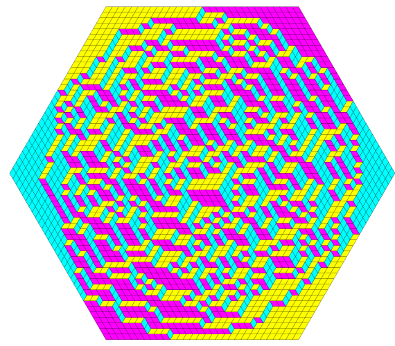
Figure 3: Boxed plane partition.

In [4] it was shown that, for a random tiling of the hexagon, the asymptotic height function $\bar{h}$ is linear outside of the inscribed circle and analytic inside (with an explicit but somewhat complicated formula). Although our theorem does not apply to this case because of the facets outside the inscribed circle, if we choose boundary conditions inside the inscribed circle, and boundary values equal to the graph of the function there, our results apply. Suppose that the hexagon has sides of length $1$, so that the inscribed circle has radius $\sqrt{3}/2$. Let $U$ be a disk of radius $r<\sqrt{3}/2$ concentric with it. Suppose that the normalized height function on the boundary of $U$ is chosen to agree with the asymptotic height function of the corresponding region in the BPP, so that the asymptotic height function of $U$ equals the asymptotic height function of the BPP restricted to $U$. Then the fluctuations on $U$ can be computed using Theorem 7.1. In fact in this setting, the conformal structure can be explicitly computed: take the standard conformal structure on a hemisphere in ${\mathbb{R}}^{3}$, and project it orthogonally onto the plane containing its equator. Identifying the equator with the inscribed circle in the BPP gives the relevant conformal structure in $U$. Remarkably, in this example the Beltrami coefficient is rotationally invariant, even though $\bar{h}$ itself is not. See section 8.

We conjecture that the fluctuations for the BPP are given by the limit $r\to\sqrt{3}/2$ of this construction (it is known [4] that fluctuations in the “frozen” regions outside the circle are exponentially small in $1/\epsilon$).

1.6 Proof outline

The fundamental tool in the study of the dimer model is the Kasteleyn matrix (defined below). Minors of the inverse Kasteleyn matrix compute edge correlations in the model. The main goal of the paper is to obtain an asymptotic expansion of the inverse Kasteleyn matrix. This is complicated by the fact that it grows exponentially in the distance between vertices (except in the special case when the boundary height function is horizontal). However by pre- and post-composition with an appropriate diagonal matrix, we can remove the exponential growth and relate $K^{-1}$ to the standard Green’s function with Dirichlet boundary conditions on a related graph ${\cal G}_{T}$.

Here is a sketch of the main ideas.

1. We construct a discrete version of the map $f$ of Theorem 1.4. For each $\epsilon$ we define a directed graph ${\cal G}_{T}$ embedded in the upper half plane ${\mathbb{H}}$, and a geometric map $\phi$ from $U_{\epsilon}$ to ${\cal G}_{T}$, such that the Laplacian on ${\cal G}_{T}$ is related (via the construction of [13, 14]) with the Kasteleyn matrix on $U_{\epsilon}$. The existence of such a graph ${\cal G}_{T}$ follows from [14]. This is done in section 3.1 in the “constant slope” case and section 4.3 in the general case.

2. Standard techniques for discrete harmonic functions yield an asymptotic expansion for the Green’s function on ${\cal G}_{T}$. This is done in section 2.6.4.

3. The asymptotic expansion of the inverse Kasteleyn matrix on $U_{\epsilon}$ is obtained from the derivative of the Green’s function on ${\cal G}_{T}$, pulled back under the mapping $\phi$. See sections 2.6.4 and 6.

4. Asymptotic expansions of the moments of the height fluctuations are computed via integrals of the asymptotic inverse Kasteleyn matrix. These moments are the moments of the Gaussian free field on ${\mathbb{H}}$ pulled back under $\phi$.

Acknowledgments. Many ideas in this paper were inspired by conversations with Henry Cohn, Jim Propp, Jean-René Geoffroy, Scott Sheffield, Béatrice deTilière, Cédric Boutillier, and Andrei Okounkov. We thanks the referees for useful comments. This paper was partially completed while the author was visiting Princeton University.

2 Definitions

2.1 Graphs

Let $\pi_{111}$ be the orthogonal projection of ${\mathbb{R}}^{3}$ onto $P_{111}$. Let $\hat{x},\hat{y},\hat{z}$ be the $\pi_{111}$-projections of the unit basis vectors. Define $e_{1}=\frac{1}{3}(\hat{x}-\hat{z}),e_{2}=\frac{1}{3}(\hat{y}-\hat{x}),e_{3}=\frac{1}{3}(\hat{z}-\hat{y}),$ so that $\hat{x}=e_{1}-e_{2},\hat{y}=e_{2}-e_{3},\hat{z}=e_{3}-e_{1}$. Let ${\cal H}$ be the honeycomb lattice in $P_{111}$: vertices of ${\cal H}$ are $L\cup(L+e_{1})$, where $L$ is the lattice $L={\mathbb{Z}}(e_{1}-e_{2})+{\mathbb{Z}}(e_{2}-e_{3})={\mathbb{Z}}\hat{x}+{\mathbb{Z}}\hat{y},$ and edges connect nearest neighbors. Vertices in $L$ are colored white, those in $L+e_{1}$ are black. See Figure 4.

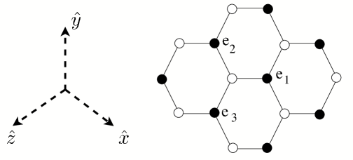
Figure 4: The honeycomb graph.

2.1.1 Dual graph

Let $U$ be a Jordan domain in $P_{111}$ with smooth boundary. In $\epsilon{\cal H}$, take a simple closed polygonal path with approximates $\partial U$ in a reasonable way, for example the polygonal curve is locally monotone in the same direction as the curve $\partial U$. Let ${\cal G}$ be the subgraph of $\epsilon{\cal H}$ bounded by this polygonal path. We define a special kind of dual graph ${\cal G}^{*}$ as follows. Let $\epsilon{\cal H}^{*}$ be the usual planar dual of $\epsilon{\cal H}$. For each white vertex of ${\cal G}$ take the corresponding triangular face of $\epsilon{\cal H}^{*}$; the union of the edges forming these triangles, along with the corresponding vertices, forms ${\cal G}^{*}$. In other words, ${\cal G}^{*}$ has a face for each white vertex of ${\cal G}$, as well as for black vertices which have all three neighbors in ${\cal G}$. See Figure 5.

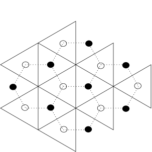
Figure 5: The “dual” graph ${\cal G}^{*}$ (solid lines) of the graph ${\cal G}$ of Figure 4.

Throughout the paper the graph ${\cal G}$ and its related graphs will be scaled by a factor $\epsilon$ over the corresponding graphs ${\cal H}$, and so the ${\cal G}$ graphs have edge lengths of order $\epsilon$, and the graph ${\cal H}$ and its related graphs have edge lengths of order $1$.

2.1.2 Forms

For an edge in ${\cal G}$ joining vertices $\mathsf{b}$ and $\mathsf{w}$, we denote by $(\mathsf{b}\mathsf{w})^{*}$ the dual edge in ${\cal G}^{*}$, which we orient at $+90^{\circ}$ from the edge $\mathsf{b}\mathsf{w}$ (when this edge is oriented from $\mathsf{b}$ to $\mathsf{w}$).

A $1$-form $\omega$ on a graph is a function on directed edges which is antisymmetric with respect to reversing the orientation: $\omega(v_{1}v_{2})=-\omega(v_{2}v_{1})$. A $1$-form is also called a flow. If the graph is planar one can similarly define a $1$-form on the dual graph. If $\omega$ is a $1$-form, $\omega^{*}$ is the dual $1$-form, defined by $\omega^{*}((v_{1}v_{2})^{*}):=\omega(v_{1}v_{2})$.

On a planar graph with a $1$-form $\omega$, $d\omega$ is a function on oriented faces defined by $d\omega(f)=\sum_{e}\omega(e)$ where the sum is over the edges on a path around the face going counterclockwise. This is also known as the curl of the flow $\omega$. The form $d\omega^{*}$ is a function on vertices (faces of the dual graph), defined by $d\omega^{*}(v)=\sum_{v^{\prime}\sim v}\omega(v,v^{\prime})$. In other words it is the divergence of the flow $\omega$.

A $1$-form $\omega$ is closed if $d\omega=0$, that is, the sum of $\omega$ along any cycle is zero (in the language of flows, the flow has zero curl). If is exact if $\omega=df$ for some function $f$ on the vertices, that is $\omega(v_{1}v_{2})=f(v_{1})-f(v_{2}).$ A $1$-form is co-closed if its dual form is closed. The corresponding flow is divergence-free.

If $d\omega^{*}=0$, the integral of $\omega^{*}$ between two faces of ${\cal G}$ (i.e. on a path in the dual graph) is the flux, or total flow, between those faces.

2.2 Heights and asymptotics

The unnormalized height function, or just height function, of a tiling is the integer-valued function on the vertices of the lozenges (faces of ${\cal G}$) which is the sum of the coordinates of the corresponding point in ${\mathbb{Z}}^{3}$. It changes by $\pm 1$ along each edge of a tile. When we scale the lattice by $\epsilon$, so that we are discussing surfaces in $\epsilon{\mathbb{Z}}^{3}$, the height function is defined as $1/\epsilon$ times the coordinate sum, so that it is still integer-valued. The normalized height function is $\epsilon$ times the height function, and is the function which, when scaled by $\sqrt{3}$, has graph which is the surface in $\epsilon{\mathbb{Z}}^{3}$.

Let $u:\partial U\to{\mathbb{R}}$ be a continuous function with the property that $u$ can be extended to a Lipschitz function $\tilde{u}$ on the interior of $U$ having the property that the normal to the graph of $\tilde{u}$ has nonnegative coordinates, that is, the normal points into the positive orthant ${\mathbb{R}}_{\geq 0}^{3}$. In other words, the graph of $u$ is a wire frame $\gamma$ of the type discussed before.

Let $\bar{h}\colon U\to{\mathbb{R}}$ be the asymptotic height function with boundary values $u$, from Theorem 1.1. It is smooth assuming the hypothesis of Theorem 1.4.

Let $\nu=(p_{a},p_{b},p_{c})$ be the normal vector to the graph of $\bar{h}$, scaled so that $p_{a}+p_{b}+p_{c}=1$. The directional derivatives of $\bar{h}$ in the directions $\hat{x},\hat{y},\hat{z}$ are respectively

$$3p_{c}-1,3p_{a}-1,3p_{b}-1.$$ (3)

2.3 Measures and gauge equivalence

We let $\mu=\mu({\cal G})$ be the uniform measure on dimer configurations on a finite graph ${\cal G}$.

If edges of ${\cal G}$ are given positive real weights, we can define a new probability measure, the Boltzmann measure, giving a configuration a probability proportional to the product of its edge weights.

Certain edge-weight functions lead to the same Boltzmann measure: in particular if we multiply by a constant the weights of all the edges in ${\cal G}$ having a fixed vertex, the Boltzmann measure does not change, since exactly one of these weights is used in every configuration. More generally, two weight functions $\nu_{1},\nu_{2}$ are said to be gauge equivalent if $\nu_{1}/\nu_{2}$ is a product of such operations, that is, if there are functions $F_{1}$ on white vertices and $F_{2}$ on black vertices so that for each edge $\mathsf{w}\mathsf{b}$, $\nu_{1}(\mathsf{w}\mathsf{b})/\nu_{2}(\mathsf{w}\mathsf{b})=F_{1}(\mathsf{w})F_{2}(\mathsf{b}).$ Gauge equivalent weights define the same Boltzmann measure.

It is not hard to show that for planar graphs, two edge-weight functions are gauge equivalent if and only if they have the same face weights, where the weight of a face is defined to be the alternating product of the edge weights around the face (that is, the first, divided by the second, times the third, and so on), see e.g. [12].

In this paper we will only consider weights which are gauge equivalent to constant weights (or nearly so), so the Boltzmann measure will always be (nearly) the uniform measure.

2.4 Kasteleyn matrices

Kasteleyn showed that one can count dimer configurations on planar graph with the determinant of the certain matrix, the “Kasteleyn matrix” [6]. In the current case, when the underlying graph is part of the honeycomb graph, the Kasteleyn matrix $K$ is just the adjacency matrix from white vertices to black vertices.

For more general bipartite planar graphs, and when the edges have weights, the matrix is a signed, weighted version of the adjacency matrix [16], whose determinant is the sum of the weights of dimer coverings. Each entry $K(\mathsf{w},\mathsf{b})$ is a complex number with modulus given by the corresponding edge weight (or zero if the vertices are not adjacent), and an argument which must be chosen in such a way that around each face the alternating product of the entries (the first, divided by the second, times the third, and so on) is positive if the face has $2\bmod 4$ edges and negative if the face has $0\bmod 4$ edges (since we are assuming the graph is bipartite, each face has an even number of edges. For nonbipartite graphs, a more complicated condition is necessary).

The Kasteleyn matrix is unique up to gauge transformations, which consist of pre- and post-multiplication by diagonal matrices (with, in general, complex entries). If the weights are real then we can choose a gauge in which $K$ is real, although in certain cases it is convenient to allow complex numbers (we will below).

Probabilities of individual edges occurring in a random tiling can likewise be computed using the minors of the inverse Kasteleyn matrix:

Theorem 2.1 ([7])

The probability of edges $\{(\mathsf{b}_{1},\mathsf{w}_{1}),\dots,(\mathsf{b}_{k},\mathsf{w}_{k})\}$ occurring in a random dimer covering is

$$\left(\prod_{i=1}^{k}K(\mathsf{w}_{i},\mathsf{b}_{i})\right)\det\{K^{-1}(\mathsf{b}_{i},\mathsf{w}_{j})\}_{1\leq i,j\leq k}.$$

On an infinite graph $K$ is defined similarly but $K^{-1}$ is not unique in general. This is related to the fact that there are potentially many different measures which could be obtained as limits of Boltzmann measures on sequences of finite graphs filling out the infinite graph. The edge probabilities for these measures can all be described as in the theorem above, but where the matrix “$K^{-1}$” now depends on the measure; see the next section for examples.

2.5 Measures in infinite volume

On the infinite honeycomb graph ${\cal H}$ there is a two-parameter family of natural translation-invariant and ergodic probability measures on dimer configurations, which restrict to the uniform measure on finite regions (i.e. when conditioned on the complement of the finite region: we say they are conditionally uniform). Such measures are also known as ergodic Gibbs measures. They are classified in the following theorem due to Sheffield.

Theorem 2.2 ([18])

For each $\nu=(p_{a},p_{b},p_{c})$ with $p_{a},p_{b},p_{c}\geq 0$ and scaled so that $p_{a}+p_{b}+p_{c}=1$ there is a unique translation-invariant ergodic Gibbs measure $\mu_{\nu}$ on the set of dimer coverings of ${\cal H}$, for which the height function has average normal $\nu$. This measure can be obtained as the limit as $n\to\infty$ of the uniform measure on the set of those dimer coverings of ${\cal H}_{n}={\cal H}/nL$ whose proportion of dimers in the three orientations is $(p_{a}:p_{b}:p_{c})$, up to errors tending to zero as $n\to\infty$. Moreover every ergodic Gibbs measure on ${\cal H}$ is of the above type for some $\nu$.

The unicity in the above statement is a deep and important result.

Associated to $\mu_{\nu}$ is an infinite matrix, the inverse Kasteleyn matrix of $\mu_{\nu}$, $K^{-1}_{\nu}=(K^{-1}_{\nu}(\mathsf{b},\mathsf{w}))$ whose rows index the black vertices and columns index the white vertices, and whose minors give local statistics for $\mu_{\nu}$, just as in Theorem 2.1. From [12] there is an explicit formula for $K_{\nu}^{-1}$: let $\mathsf{w}=m_{1}\hat{x}+n_{1}\hat{y}$ and $\mathsf{b}=e_{1}+m_{2}\hat{x}+n_{2}\hat{y}=\mathsf{w}+e_{1}+m\hat{x}+n\hat{y}$ where $m=m_{2}-m_{1},n=n_{2}-n_{1}$. Then

$$K^{-1}_{\nu}(\mathsf{b},\mathsf{w})=a(\frac{a}{b})^{m}(\frac{b}{c})^{n}K^{-1}_{abc}(\mathsf{b},\mathsf{w}),$$ (4)

where $a,b,c,z,w$ are as defined in section (1.2.3) and

$$K^{-1}_{abc}(\mathsf{b},\mathsf{w}) = \frac{1}{(2\pi i)^{2}}\int_{|z|=|w|=1}\frac{z_{1}^{-m+n}w_{1}^{-n}}{a+bz_{1}+cw_{1}}\frac{dz_{1}}{z_{1}}\frac{dw_{1}}{w_{1}}$$ (5)

$$= \frac{1}{\pi}{\rm{Im}}\left(\frac{z^{-m+n}w^{-n}}{cwm+an}\right)+O\left(\frac{1}{m^{2}+n^{2}}\right).$$ (6)

This formula for $K_{abc}^{-1}$ and its asymptotics were derived in [12]: they are obtained from the limit $n\to\infty$ of the inverse Kasteleyn matrix on the torus ${\cal H}/nL$ with edge weights $a,b,c$ according to direction. It is not hard to check from (5) that $KK^{-1}=Id$

From (4), the matrix $K_{\nu}^{-1}$ is just a gauge transformation of $K_{abc}^{-1}$, that is, obtained by pre- and post-composing with diagonal matrices.

Defining $F(\mathsf{w})=(bz/a)^{m_{1}}(cw/bz)^{n_{1}}$ and $F(\mathsf{b})=a(bz/a)^{-m_{2}}(cw/bz)^{-n_{2}}$ we can write, using (6),

$$K^{-1}_{\nu}(\mathsf{b},\mathsf{w})=\frac{1}{\pi}{\rm{Im}}\left(\frac{F(\mathsf{w})F(\mathsf{b})}{cwm+an}\right)+|F(\mathsf{b})F(\mathsf{w})|O(\frac{1}{m^{2}+n^{2}}).$$ (7)

We’ll use this function $F$ below.

As a sample calculation, the $\mu_{\nu}$-probability of a single horizontal edge, from $\mathsf{w}=0$ to $\mathsf{b}=e_{1}$, being present in a random dimer covering is (see Theorem 2.1)

$$K_{\nu}^{-1}(\mathsf{b},\mathsf{w})=aK_{abc}^{-1}(\mathsf{b},\mathsf{w})=\frac{a}{(2\pi i)^{2}}\int_{{\mathbb{T}}^{2}}\frac{1}{a+bz_{1}+cw_{1}}\frac{dz_{1}}{z_{1}}\frac{dw_{1}}{w_{1}}=\frac{\theta_{a}}{\pi},$$

where $\theta_{a}$ is, as before, the angle opposite side $a$ in a triangle with sides $a,b,c$. This is consistent with (3).

2.6 $T$-graphs

2.6.1 Definition

$T$-graphs were defined and studied in [14]. A pairwise disjoint collection $L_{1},L_{2},\ldots,L_{n}$ of open line segments in ${\mathbb{R}}^{2}$ forms a T-graph in ${\mathbb{R}}^{2}$ if $\cup_{i=1}^{n}L_{i}$ is connected and contains all of its limit points except for some finite set $R=\{r_{1},\ldots,r_{m}\}$, where each $r_{i}$ lies on the boundary of the infinite component of ${\mathbb{R}}^{2}$ minus the closure of $\cup_{i=1}^{n}L_{i}$. See Figure 6 for an example where the outer boundary is a polygon. Elements in $R$ are called root vertices and are labeled in cyclic order; the $L_{i}$ are called complete edges. We only consider the case that the outer boundary of the $T$-graph is a simple polygon, and the root vertices are the convex corners of this polygon. (An example where the outer boundary is not a polygon is a “T” formed from two edges, one ending in the interior of the other.)

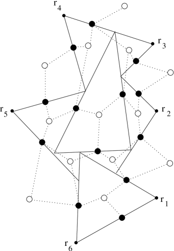
Figure 6: A T-graph (solid) and associated graph ${\cal G}_{D}$ (dotted).

Associated to a $T$-graph is a Markov chain ${\cal G}_{T}$, whose vertices are the points which are endpoints of some $L_{i}$. Each non-root vertex is in the interior of a unique $L_{j}$ (because the $L_{j}$ are disjoint); there is a transition from that vertex to its adjacent vertices along $L_{j}$, and the transition probabilities are proportional to the inverses of the Euclidean distances. Root vertices are sinks of the Markov chain. See Figure 7.

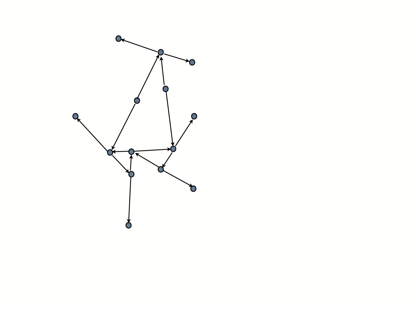
Figure 7: The Markov chain associated to the $T$-graph of Figure 6. Note that root vertices are sinks of the Markov chain.

Note that the coordinate functions on ${\cal G}_{T}$ are harmonic functions on ${\cal G}_{T}\setminus R$. More generally, any function $f$ on ${\cal G}_{T}$ which is harmonic on ${\cal G}_{T}\setminus R$ (we refer to such functions as harmonic functions on ${\cal G}_{T}$) has the property that it is linear along edges, that is, if $v_{1},v_{2},v_{3}$ are vertices on the same complete edge then

$$\frac{f(v_{1})-f(v_{2})}{v_{1}-v_{2}}=\frac{f(v_{2})-f(v_{3})}{v_{2}-v_{3}}.$$ (8)

2.6.2 Associated dimer graph and Kasteleyn matrix

Associated to a $T$-graph is a weighted bipartite planar graph ${\cal G}_{D}$ constructed as follows, see Figure 6. Black vertices of ${\cal G}_{D}$ are the $L_{j}$. White vertices are the bounded complementary regions, as well as one white vertex for each boundary path joining consecutive root vertices $r_{j}$ and $r_{j+1}$ (but not for the path from $r_{m}$ to $r_{1}$). The complementary regions are called faces; the paths between adjacent root vertices are called outer faces. Edges connect the $L_{i}$ to each face it borders along a positive-length subsegment. The edge weights are equal to the Euclidean length of the bounding segment.

To ${\cal G}_{D}$ there is a canonically associated Kasteleyn matrix of ${\cal G}_{D}$: this is the $n\times n$ matrix $K_{{\cal G}_{D}}=(K_{{\cal G}_{D}}(\mathsf{w},\mathsf{b}))$ with rows indexing the white vertices and columns indexing the black vertices of ${\cal G}_{D}$. We have $K_{{\cal G}_{D}}(\mathsf{w},\mathsf{b})=0$ if $\mathsf{w}$ and $\mathsf{b}$ are not adjacent, and otherwise $K_{{\cal G}_{D}}(\mathsf{w},\mathsf{b})$ is the complex number equal to the edge vector corresponding to the edge of the region $\mathsf{w}$ along complete edge $\mathsf{b}$ (taken in the counterclockwise direction around $\mathsf{w}$). In particular $|K_{{\cal G}_{D}}(\mathsf{w},\mathsf{b})|$ is the length of the corresponding edge of $\mathsf{w}$.

Lemma 2.3

$K_{{\cal G}_{D}}$ is a Kasteleyn matrix for ${\cal G}_{D}$, that is, the alternating product of the matrix entries for edges around a bounded face is positive real or negative real according to whether the face has $2\bmod 4$ or $0\bmod 4$ edges, respectively.

By alternating product we mean the first, divided by the second, times the third, etc.

Proof:     Let $f$ be a bounded face of ${\cal G}_{D}$ (we mean not one of the outer faces). It corresponds to a meeting point of two or more complete edges; this meeting point is in the interior of exactly one of these complete edges, $L$. See Figure 8. In ${\cal G}_{D}$, for each other black vertex on that face the two edges of the $T$-graph to neighboring white vertices have opposite orientations. The two edges parallel to $L$ (horizontal in the figure) have the same orientation, so their ratio is positive. This implies the result. $\square$

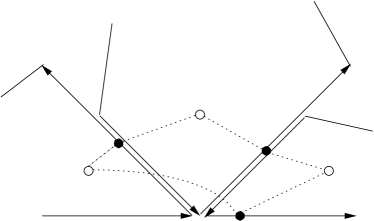
Figure 8: A face of ${\cal G}_{D}$ (dotted).

Although we won’t need this fact, in [14] it is shown that the set in-directed spanning forests of ${\cal G}_{T}$ (rooted at the root vertices and weighted by the product of the transition probabilities) is in measure-preserving (up to a global constant) bijection with the set of dimer coverings of ${\cal G}_{D}$.

2.6.3 Harmonic functions and discrete analytic functions

To a harmonic function $f$ on a $T$-graph ${\cal G}_{T}$ we associate a derivative $df$ which is a function on black vertices of ${\cal G}_{D}$ as follows. Let $v_{1}$ and $v_{2}$ be two distinct points on complete edge $\mathsf{b}$, considered as complex numbers. We define

$$df(\mathsf{b})=\frac{f(v_{2})-f(v_{1})}{v_{2}-v_{1}}.$$ (9)

Since $f$ is linear along any complete edge (equation (8)), $df$ is independent of the choice of $v_{1}$ and $v_{2}$.

Lemma 2.4

If $f$ is harmonic on a $T$-graph ${\cal G}_{T}$ and $K=K_{{\cal G}_{D}}$ is the associated Kasteleny matrix, then $\sum_{\mathsf{b}\in B}K(\mathsf{w},\mathsf{b})df(\mathsf{b})=0$ for any interior white vertex $\mathsf{w}$.

Proof:     Let $\mathsf{b}_{1},\dots,\mathsf{b}_{k}$ be the neighbors of $\mathsf{w}$ in cyclic order. To each neighbor $\mathsf{b}_{i}$ is associated a segment of a complete edge $L_{i}$. Let $v_{i}$ and $v_{i+1}$ be the endpoints of that segment, and $w_{i}$ and $w_{i}^{\prime}$ be the endpoints of $L_{i}$. Then

$$\frac{f(v_{i+1})-f(v_{i})}{v_{i+1}-v_{i}}=\frac{f(w_{i}^{\prime})-f(w_{i})}{w_{i}^{\prime}-w_{i}}$$

since the harmonic function is linear along $L_{i}$. In particular

$$K_{{\cal G}_{D}}(\mathsf{w},\mathsf{b}_{i})df(\mathsf{b}_{i})=(v_{i+1}-v_{i})\frac{f(w_{i}^{\prime})-f(w_{i})}{w_{i}^{\prime}-w_{i}}=f(v_{i+1})-f(v_{i}).$$

Summing over $i$ (with cyclic indices) yields the result. $\square$

Note that at a boundary white vertex $\mathsf{w}$, $\sum_{B}K_{{\cal G}_{D}}(\mathsf{w},\mathsf{b})df(\mathsf{b})$ is the difference in $f$-values at the adjacent root vertices of ${\cal G}_{T}$.

We will refer to a function $g$ on black vertices of ${\cal G}_{D}$ satisfying $\sum_{\mathsf{b}\in B}K_{{\cal G}_{D}}(\mathsf{w},\mathsf{b})g(\mathsf{b})=0$ for all interior white vertices $\mathsf{w}$ as a discrete analytic function.

The construction in the above lemma can be reversed, starting from a discrete analytic function $df$ (on black vertices of ${\cal G}_{D}$) and integrating to get a harmonic function $f$ on ${\cal G}_{T}$: define $f$ arbitrarily at a vertex of ${\cal G}_{T}$ and then extend to neighboring vertices (on a same complete edge) using (9). The extension is well-defined by discrete analyticity.

2.6.4 Green’s function and $K_{{\cal G}_{D}}^{-1}$

We can relate $K_{{\cal G}_{D}}^{-1}$ to the conjugate Green’s function on ${\cal G}_{T}$ using the construction of the previous section, as follows.

Let $\mathsf{w}$ be an interior face of ${\cal G}_{T}$, and $\ell$ a path from a point in $\mathsf{w}$ to the outer boundary of ${\cal G}_{T}$ which misses all the vertices of ${\cal G}_{T}$. For vertices $v$ of ${\cal G}_{T}$, define the conjugate Green’s function $G^{*}(\mathsf{w},v)$ to be the expected algebraic number of crossings of $\ell$ by the random walk started at $v$ and stopped at the boundary. This is the unique function with zero boundary values which is harmonic everywhere except for a jump discontinuity of $-1$ across $\ell$ when going counterclockwise around $\mathsf{w}$. (If there were two such functions, their difference would be harmonic everywhere with zero boundary values. ) See Figure 9 for an example.

Let $K_{{\cal G}_{D}}^{-1}(\mathsf{b},\mathsf{w})$ be the discrete analytic function of $\mathsf{b}$ defined from $G^{*}(\mathsf{w},v)$ as in the previous section; on an edge which crosses $\ell$, define $K_{{\cal G}_{D}}^{-1}(\mathsf{b},\mathsf{w})$ using two points on $\mathsf{b}$ on the same side of $\ell$. This function clearly satisfies $K_{{\cal G}_{D}}K_{{\cal G}_{D}}^{-1}=I$ by Lemma 2.4, and therefore is independent of the choice of $\ell$.

Note that $K_{{\cal G}_{D}}^{-1}$ also has the following probabilistic interpretation: take two particles, started simultaneously at two different points $v_{1},v_{2}$ of the same complete edge, and couple their random walks so that they start independently, take simultaneous steps, and when they meet they stick together for all future times. Then the difference in their winding numbers around $\mathsf{w}$ is determined by their crossings of $\ell$ before they meet. That is, $K_{{\cal G}_{D}}^{-1}(\mathsf{b},\mathsf{w})(v_{1}-v_{2})$ is the expected difference in crossings before the particles meet or until they hit the boundary, whichever comes first.

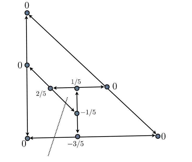
Figure 9: Conjugate Green’s function example. Here the sides of the triangle are bisected in ratio $2:3$ and interior complete edges $1:1$.

3 Constant-slope case

In this section we compute the asymptotic expansion of $K^{-1}_{{\cal G}_{D}}$ (Theorem 3.7) in the special case is when $\gamma$ is planar. In this case the normalized asymptotic height function $\bar{h}$ is linear, and its normal $\nu$ is constant. This case already contains most of the complexity of the general case, which is treated in section 4.

Let $\nu=(p_{a},p_{b},p_{c})$ be the normal to $\bar{h}$, scaled as usual so that $p_{a}+p_{b}+p_{c}=1$. The angles $\theta_{a},\theta_{b},\theta_{c}$ are constant, and we choose $a,b,c$ as before to be constant as well. Define a function

$$F(\mathsf{w})=(bz/a)^{m}(cw/bz)^{n}$$

at a white vertex $\mathsf{w}=m\hat{x}+n\hat{y}$ and

$$F(\mathsf{b})=a(bz/a)^{-m}(cw/bz)^{-n}$$

at a black vertex $\mathsf{b}=e_{1}+m\hat{x}+n\hat{y}$. These functions are defined on all of the honeycomb graph ${\cal H}$. Let $K_{\cal H}$ be the adjacency matrix of ${\cal H}$ (which, as we mentioned earlier, is a Kasteleyn matrix for ${\cal H}$).

Lemma 3.1

We have

$$\sum_{\mathsf{b}}K_{\cal H}(\mathsf{w},\mathsf{b})F(\mathsf{b})=0=\sum_{\mathsf{w}}F(\mathsf{w})K_{\cal H}(\mathsf{w},\mathsf{b})$$ (10)

where $K_{\cal H}$ is the adjacency matrix of ${\cal H}$.

Proof:     This follows from the equation $a+bz+cw=0$. $\square$

3.1 $T$-graph construction

Define a $1$-form $\Omega$ on edges of ${\cal H}$ by

$$\Omega(\mathsf{w}\mathsf{b})=-\Omega(\mathsf{b}\mathsf{w})=2{\rm{Re}}(F(\mathsf{w}))F(\mathsf{b}).$$ (11)

By (10) the dual form $\Omega^{*}$ (defined by $\Omega^{*}((\mathsf{w}\mathsf{b})^{*})=\Omega(\mathsf{w}\mathsf{b})$) is closed (the integral around any closed cycle is zero) and therefore $\Omega^{*}=d\Psi$ for a complex-valued function $\Psi$ on ${\cal H}^{*}$. Here ${\cal H}^{*}$, the dual of the honeycomb, is the graph of the equilateral triangulation of the plane. Extend $\Psi$ linearly over the edges of ${\cal H}^{*}$. This defines a mapping from ${\cal H}^{*}$ to ${\mathbb{C}}$ with the property that the images of the white faces are triangles similar to the $a,b,c$-triangle (via orientation-preserving similarities), and the images of black faces are segments. This follows immediately from the definitions: if $\mathsf{b}_{1},\mathsf{b}_{2},\mathsf{b}_{3}$ are the three neighbors of a white vertex $\mathsf{w}$ of ${\cal H}$, the edges $\mathsf{w}\mathsf{b}_{i}$ have values $2{\rm{Re}}(F(\mathsf{w}))F(\mathsf{b}_{i})$ which are proportional to $F(\mathsf{b}_{1}):F(\mathsf{b}_{2}):F(\mathsf{b}_{3})$, which in turn are proportional to $a:bz:cw$ by (10). If $\mathsf{w}_{1},\mathsf{w}_{2},\mathsf{w}_{3}$ are the three neighbors of a black vertex then the corresponding edge values are $2{\rm{Re}}(F(\mathsf{w}_{i}))F(\mathsf{b})$ which are proportional to ${\rm{Re}}(F(\mathsf{w}_{1})):{\rm{Re}}(F(\mathsf{w}_{2})):{\rm{Re}}(F(\mathsf{w}_{3}))$, that is, they all have the same slope and sum to zero.

It is not hard to see that the images of the white triangles are in fact non-overlapping (see [14], Section 5 for the proof, or look at Figure 10). It may be that ${\rm{Re}}F(\mathsf{w})=0$ for some $\mathsf{w}$; in this case choose a generic modulus-$1$ complex number $\lambda$ and replace $F(\mathsf{w})$ by $\lambda F(\mathsf{w})$ and $F(\mathsf{b})$ by $\overline{\lambda}F(\mathsf{b})$. So we can assume that each white triangle is similar to the $a,b,c$-triangle. In fact, this operation will be important later; note that by varying $\lambda$ the size of an individual triangle varies; by an appropriate choice we can make any particular triangle have maximal size (side lengths $a,b,c$).

Figure 10: The $\Psi$-image of ${\cal H}^{*}$ is a $T$-graph covering ${\mathbb{R}}^{2}$

Lemma 3.2

The mapping $\Psi$ is almost linear, that is, it is a linear map $\phi(m,n)=cwm+an$ plus a bounded function.

Proof:     Consider for example a vertical column of horizontal edges $\{\mathsf{w}_{1}\mathsf{b}_{1},\dots,\mathsf{w}_{k}\mathsf{b}_{k}\}$ of ${\cal H}$ connecting a face $f_{1}$ to face $f_{k+1}$. We have

$$\sum_{i=1}^{k}\Omega^{*}((\mathsf{w}_{i}\mathsf{b}_{i})^{*}) = \sum_{i=1}^{k}\Omega(\mathsf{w}_{i}\mathsf{b}_{i})$$

$$= \sum_{i=1}^{k}(F(\mathsf{w}_{i})+\overline{F(\mathsf{w}_{i})})F(\mathsf{b}_{i})$$

$$= ka+\sum_{i=1}^{k}\overline{F(\mathsf{w}_{i})}F(\mathsf{b}_{i})$$

$$= ka+a\sum_{i=1}^{k}z^{2i}w^{-2i}$$

$$= \phi(f_{k+1})-\phi(f_{1})+osc,$$

where $osc$ is oscillating and in fact $O(1)$ independently of $k$ (by hypothesis $z/w\not\in{\mathbb{R}}$). In the other two lattice directions the linear part of $\Psi$ is again $\phi$, so that $\Psi$ is almost linear in all directions. $\square$

This lemma shows that the image of ${\cal H}^{*}$ under $\Psi$ is an infinite $T$-graph ${\cal H}_{T}$ covering all of ${\mathbb{R}}^{2}$. The images of the black triangles are the complete edges and have lengths $O(1)$.

If we insert a $\lambda$ as above and let $\lambda$ vary over the unit circle, one sees all possible local structures of the $T$-graph, that is, the geometry of the $T$-graph ${\cal H}_{T}={\cal H}_{T}(\lambda)$ in a neighborhood of a triangle $\Psi(\mathsf{w})$ only depends up to homothety on the argument of $\lambda F(\mathsf{w})$.

Recall that ${\cal G}^{*}$ is a subgraph of $\epsilon{\cal H}^{*}$ approximating $U$. We can restrict $\Psi$ to $\frac{1}{\epsilon}{\cal G}^{*}$ thought of as a subgraph of $\frac{1}{\epsilon}{\cal H}$, and then multiply its image by $\epsilon$. Thus we get a finite sub-$T$-graph ${\cal G}_{T}$ of $\epsilon{\cal H}_{T}$. Let $\Psi_{\epsilon}=\epsilon\circ\Phi\circ\frac{1}{\epsilon}$ so that $\Psi_{\epsilon}$ acts on ${\cal G}^{*}$.

The union of the $\Psi_{\epsilon}$-images of the white triangles in ${\cal G}^{*}$ forms a polygon $P$. Define the “dimer” graphs ${\cal H}_{D}$ associated to ${\cal H}_{T},$ and ${\cal G}_{D}$ associated to ${\cal G}_{T}$ as in section 2.6.2. See Figure 6 for the $T$-graph arising from the graph ${\cal G}^{*}$ of Figure 5. Note that ${\cal G}_{D}$ contains ${\cal G}$ (defined in section 2.1.1) but has extra white vertices along the boundaries. These extra vertices make the height function on ${\cal G}_{D}$ approximate the desired linear function (whose graph has normal $\nu$), see the next section.

From (11) we have

Lemma 3.3

Edge weights of ${\cal H}_{D}$ and ${\cal G}_{D}$ are gauge equivalent to constant edge weights. Indeed, for $\mathsf{w}$ not on the boundary of ${\cal G}_{D}$ we have

$$K_{{\cal G}_{D}}(\mathsf{w},\mathsf{b})=2\epsilon{\rm{Re}}(F(\mathsf{w}))F(\mathsf{b})K_{\cal G}(\mathsf{w},\mathsf{b})$$ (13)

and similarly for all $\mathsf{w}$,

$$K_{{\cal H}_{D}}=2{\rm{Re}}(F(\mathsf{w}))F(\mathsf{b})K_{\cal H}(\mathsf{w},\mathsf{b}).$$ (14)

Asymptotics of $K_{{\cal G}_{D}}^{-1}$ are described below in section 3.4. For $K_{{\cal H}_{D}}$, from (7) and (14) we have

$$K_{{\cal H}_{D}}^{-1}(\mathsf{b},\mathsf{w})=\frac{1}{2\pi{\rm{Re}}(F(\mathsf{w}))F(\mathsf{b})}{\rm{Im}}\left(\frac{F(\mathsf{w})F(\mathsf{b})}{\phi(\mathsf{b})-\phi(\mathsf{w})}\right)+O(\frac{1}{|\phi(\mathsf{b})-\phi(\mathsf{w})|^{2}}).$$ (15)

Here $K^{-1}_{{\cal H}_{D}}$ is the inverse constructed from the conjugate Green’s function on the $T$-graph ${\cal H}_{T}$. We use the fact that $2{\rm{Re}}(F(\mathsf{w}))F(\mathsf{b})K^{-1}_{{\cal H}_{D}}(\mathsf{b},\mathsf{w})$ coincides with $K^{-1}_{\nu}$ of (7) since both satisfy the equation that $dK^{-1}$ equals the conjugate Green’s function.

3.2 Boundary behavior

Recall that from our region $U$ we constructed a graph ${\cal G}$ (section 2.1.1). From the normalized height function $u$ on $\partial U$ (which is the restriction of a linear function to $\partial U$) we constructed the $T$-graph ${\cal G}_{T}$ and then the dimer graph ${\cal G}_{D}$.

In this section we show that the normalized boundary height function of ${\cal G}_{D}$ when ${\cal G}_{D}$ is chosen as above approximates $\bar{h}$. This is proved in a roundabout way: we first show that the boundary height does not depend (up to local fluctuations) on the exact choice of boundary conditions, as long as we construct ${\cal G}_{T}$ from ${\cal G}^{*}$ as in section 2.1. Then we compute the height change for “simple” boundary conditions.

3.2.1 Flows and dimer configurations

Any dimer configuration $m$ defines a flow (or $1$-form) $[m]$ with divergence $1$ at each white vertex and divergence $-1$ at each black vertex: just flow by $1$ along each edge in $m$ and $0$ on the other edges.

The set $\Omega_{1}\subset[0,1]^{E}$ of unit white-to-black flows (i.e. flows with divergence $1$ at each white vertex and $-1$ at each black vertex) and with capacity $1$ on each edge is a convex polytope whose vertices are the dimer configurations [15]. On the graph ${\cal H}$ define the flow $\omega_{1/3}\in\Omega_{1}$ to be the flow with value $1/3$ on each edge $\mathsf{w}\mathsf{b}$ from $\mathsf{w}$ to $\mathsf{b}$. Up to a factor $1/3$, this flow can be used to define the height function, in the sense that for any dimer configuration $m$, $[m]-\omega_{1/3}$ is a divergence-free flow and the integral of its dual (which is closed) is $1/3$ times the height function of $m$. That is, the height difference between two points is three times the flux of $[m]-\omega_{1/3}$ between those points. This is easy to see: across an edge which contains a dimer the height changes by $\pm 2$ (depending on the orientation); if the edge does not contain a dimer the height changes by $\mp 1$, for so that the height change can be written $\pm(3\chi-1)$ where $\chi$ is the indicator function of a dimer on that edge.

For a finite subgraph of ${\cal H}$ the boundary height function can be obtained by integrating around the boundary ($3$ times) the dual of $[m]-\omega_{1/3}$ for some $m$.

3.2.2 Canonical flow

On ${\cal H}_{D}$ there is a canonical flow $\omega\in\Omega_{1}$ defined as illustrated in Figure 11: let $v_{1}v_{2}$ be the two vertices of ${\cal G}_{T}$ along $\mathsf{b}$ adjacent to $\mathsf{w}$. The flow from $\mathsf{w}$ to $\mathsf{b}$ is $1/(2\pi)$ times the sum of the two angles that the complete edges through $v_{1}$ and $v_{2}$ make with $\mathsf{b}$. One or both of these angles may be zero.

Note that the total flow out of $\mathsf{w}$ is $1$. For an edge $\mathsf{b}$, the total flow into $\mathsf{b}$ is also $1$ as illustrated on the right in Figure 11.

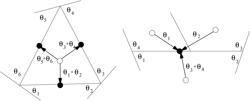
Figure 11: Defining the canonical flow (divide the angles by $2\pi$).

Now ${\cal G}_{D}$ is a subgraph of ${\cal H}_{D}$ with extra white vertices around its boundary. The canonical flow on ${\cal H}_{D}$ restricts to a flow on ${\cal G}_{D}$ except on edges connecting to these extra white vertices (we define the canonical flow there to be zero). This flow has divergence $1,-1$ at white/black vertices, except at the black vertices of ${\cal G}_{D}$ connected to the boundary white vertices, and the boundary white vertices themselves. If $m$ is a dimer covering of ${\cal G}_{D}$, the flow $[m]-\omega$ is now a divergence-free flow on ${\cal G}_{D}$ except at these black and white boundary vertices.

Lemma 3.4

Along the boundary of ${\cal G}_{D}$ the divergence of $[m]-\omega$ for any dimer configuration $m$ is the turning angle of the boundary of $P$.

Proof:     Consider a complete edge $L$ corresponding to black vertex $\mathsf{b}$. The canonical flow into $\mathsf{b}$ has a contribution from the two endpoints of $L$. The flow $[m]$ can be considered to contribute $-1/2$ for each endpoint.

Recall that each endpoint of $L$ ends in the interior of another complete edge or at a convex vertex of the polygon $P$. If an endpoint of $L$ ends in the interior of another complete edge, and there are white faces adjacent to the two sides of this endpoint (that is, the endpoint is not a concave vertex of $P$) then the contribution of the canonical flow is also $-1/2$, so the contribution of $[m]-\omega$ is zero.

Suppose the endpoint is at a concave vertex $v$ of $P$ with exterior angle $\theta<\pi$. The contribution from $v$ to the flow of $[m]-\omega$ into $L$ is $-1/2+\frac{\theta}{2\pi}$. The other complete edge at $v$ does not end at $v$ and so has no contribution. This quantity is $1/2\pi$ times the turning angle of the boundary.

Suppose the endpoint is at a convex vertex $v^{\prime}$ of $P$ of interior angle $\theta<\pi$. There is some complete edge $L^{\prime}$ of ${\cal H}_{T}$, containing $v^{\prime}$ in its interior, which is not in ${\cal G}_{T}$. The sum of the contributions of $[m]-\omega$ for the endpoints of the two complete edges $L_{1},L_{2}$ of ${\cal G}_{T}$ meeting at $v^{\prime}$ is $-1/2-\theta/2\pi$. This is the $1/2\pi$ times the turning angle at the convex vertex, minus $1$.

The contribution from $[m]$ from the boundary white vertices is $1$ per white boundary vertex, that is, one per convex vertex of $P$. $\square$

This lemma proves in particular that the divergence of $[m]-\omega$ is bounded for any $[m]$.

3.2.3 Boundary height

Recall that the height function of a dimer covering $m$ can be defined as the flux of $\omega_{1/3}-[m]$. In particular, the flux of $\omega_{1/3}-\omega$ defines the boundary height function up to $O(1)$ (the turning of the boundary), since the flux of $[m]-\omega$ is the boundary turning angle.

The flux of $\omega_{1/3}-\omega$ between two faces can be computed along any path, and in fact because both $\omega_{1/3}$ and $\omega$ are locally defined from ${\cal H}_{D}$, we see that the flux does not depend on the choice of the nearby boundary. Let us compute this flux and show that it is linear along lattice directions, and therefore linear everywhere in ${\cal H}_{D}$.

Take a vertical column of horizontal edges in ${\cal G}$, and let us compute $\omega$ on this set of edges. The $\Psi$ image of the dual of this column is a polygonal curve $\eta$ whose $j$th edge is (using (3.1)) a constant times $1+(\frac{z}{w})^{2j}$. The image of the triangles in the vertical column of ${\cal G}^{*}$ is as shown in Figure 12.

Figure 12: A column of triangles from ${\cal G}_{T}$.

The $j$th edge is part of a complete edge corresponding to the $j$th black vertex in the column. By the argument of the previous section, the flux is equal to the number of convex corners of this polygonal curve $\eta$, that is, corners where the curve turns left. The curve $\eta$ has a convex corner when

$${\rm{Im}}\left(\frac{1+(z/w)^{2j+2}}{1+(z/w)^{2j}}\right)\geq 0,$$

that is, using $z/w=-e^{i\theta_{a}},$ when $2j\theta_{a}\in[\pi,\pi+2\theta_{a}].$ Assuming that $\theta_{a}$ is irrational, this happens with frequency $\frac{2\theta_{a}}{2\pi}$, so the flux of $\omega_{1/3}-\omega$ along a column of length $n$ is $n(\frac{\theta_{a}}{\pi}-\frac{1}{3})$, and the average flux per edge is $p_{a}-1/3$. Therefore the average height change per horizontal edge is $3p_{a}-1$. If $\theta_{a}$ is rational, a continuity argument shows that $3p_{a}-1$ is still the average height change per horizontal edge. A similar result holds in the other directions, and (3) show that the average height has normal $(p_{a},p_{b},p_{c})$ as desired.

3.3 Continuous and discrete harmonic functions

To understand the asymptotic expansion of $G^{*}$, the conjugate Green’s function on ${\cal G}_{T}$, from which we can get $K^{-1}$, we need two ingredients. We need to understand the conjugate Green’s function on ${\cal H}_{T}$, and also the relation between continuous harmonic functions on domains in ${\mathbb{R}}^{2}$ and discrete harmonic functions on (domains in) $\epsilon{\cal H}_{T}$.

3.3.1 Discrete and continuous Green’s functions

On ${\cal H}_{T}$, the discrete conjugate Green’s function $G^{*}(\mathsf{w},v)$, for $\mathsf{w}\in{\cal H}$ and $v\in{\cal H}_{T}$, can be obtained from integrating the exact formula for $K^{-1}_{\nu}$ given in (4) as discussed in Section 2.6.4.

As we shall see, this formula differs even in its leading term from the continuous conjugate Green’s function, due to the singularity at the diagonal. Basically, because our Markov chain is directed, a long random walk can have a nonzero expected winding number around the origin. This causes the conjugate Green’s function, which measures this winding, to have a component of ${\rm{Re}}\log v$ as well as a part ${\rm{Im}}\log v$.

The continuous conjugate Green’s function on the whole plane is

$$g^{*}(v_{1},v_{2})=\frac{1}{2\pi}{\rm{Im}}\log(v_{2}-v_{1}).$$

(We use $G^{*}$ to denote the discrete conjugate Green’s function and $g^{*}$ the continuous version.)

To compute the discrete conjugate Green’s function $G^{*}$, if we simply restrict $g^{*}$ to the vertices of $\epsilon{\cal H}_{T}$, it will be very nearly harmonic as a function of $v_{2}$ for large $|v_{2}-v_{1}|$, but the discrete Laplacian of $g^{*}$ at vertices $v_{2}$ near $v_{1}$ (within $O(\epsilon)$ of $v_{1}$) will be of constant order in general. We can correct for the non-harmonicity at a vertex $v^{\prime}$ by adding an appropriate multiple of the actual (non-conjugate) discrete Green’s function $G(v,v_{2})$. The large scale behavior of this correction term is a constant times ${\rm{Re}}\log(v_{2}-v^{\prime}).$ So we can expect the long-range behavior of the discrete conjugate Green’s function $G^{*}(\mathsf{w},v)$, for $|\mathsf{w}-v|$ large, to be equal to $g^{*}(\mathsf{w},v)$ plus a sum of terms involving the real part ${\rm{Re}}\log(v-v^{\prime})$ for $v^{\prime}$s within $O(\epsilon)$ of $\phi(\mathsf{w})$. These extra terms sum to a function of the form $c\log|v-\phi(\mathsf{w})|+\epsilon s(v)+O(\epsilon^{2}),$ where $s$ is a smooth function and $c$ is a real constant, both $c$ and $s$ depending on the local structure of ${\cal H}_{T}$ near $\phi(\mathsf{w})$.

This form of $G^{*}$ can be seen explicitly, of course, if we integrate the exact formula (15). We have

Lemma 3.5

The discrete conjugate Green’s function $G^{*}$ on the plane $\epsilon{\cal H}_{T}$ is asymptotically

$$G^{*}(\mathsf{w},v)=\frac{1}{2\pi}\left({\rm{Im}}\log(v-\phi(\mathsf{w}))+\frac{{\rm{Im}}(F(\mathsf{w}))}{{\rm{Re}}(F(\mathsf{w}))}{\rm{Re}}\log(v-\phi(\mathsf{w}))\right)+\\ +\epsilon s(\mathsf{w},v)+O(\epsilon^{2})+O(\frac{1}{|v-\phi(\mathsf{w})|})$$ (16)

$$=\frac{1}{2\pi{\rm{Re}}(F(\mathsf{w}))}{\rm{Im}}\bigl{(}F(\mathsf{w})\log(v-\phi(\mathsf{w}))\bigr{)}+\epsilon s(\mathsf{w},v)+O(\epsilon^{2})+O(\frac{1}{|v-\phi(\mathsf{w})|})$$ (17)

where $s(\mathsf{w},v)$ is a smooth function of $v$.

Proof:     From the argument of the previous paragraph, it suffices to compute the constant in front of the ${\rm{Re}}\log(v-\phi(\mathsf{w}))$ term. This can be computed by differentiating the above formula with respect to $v$ and comparing with formula (15) for $K^{-1}$. The differential of $\epsilon s(\mathsf{w},v)$ is $O(\epsilon)$. Let $v_{1},v_{2}$ be two vertices of complete edge $\mathsf{b}$, coming from adjacent faces of ${\cal H}$, adjacent across an edge $\mathsf{b}\mathsf{w}_{1}$ (so that $v_{1}-v_{2}=\Omega^{*}(\mathsf{b}\mathsf{w}_{1})=2\epsilon{\rm{Re}}(F(\mathsf{w}_{1}))F(\mathsf{b})$). We have for $\mathsf{w}$ far from $\mathsf{w}_{1}$

$$K_{{\cal H}_{D}}^{-1}(\mathsf{b},\mathsf{w}) = \frac{G^{*}(\mathsf{w},v_{1})-G^{*}(\mathsf{w},v_{2})}{v_{1}-v_{2}}$$

$$= \frac{\frac{1}{2\pi}{\rm{Im}}\left(\frac{F(\mathsf{w})}{{\rm{Re}}(F(\mathsf{w}))}\frac{v_{1}-v_{2}}{\phi(\mathsf{b})-\phi(\mathsf{w})}\right)}{2\epsilon{\rm{Re}}(F(\mathsf{w}_{1}))F(\mathsf{b})}+O(\epsilon)$$

$$= \frac{1}{2\pi{\rm{Re}}(F(\mathsf{w}))F(\mathsf{b})}{\rm{Im}}\left(\frac{F(\mathsf{w})F(\mathsf{b})}{\phi(\mathsf{b})-\phi(\mathsf{w})}\right)+O(\epsilon).$$

$\square$

Note that in fact for any complex number $\lambda$ of modulus $1$, we get a discrete conjugate Green’s function $G^{*}_{\lambda}$ on the graph $\epsilon{\cal H}_{T}(\lambda)$ (from Section 3.2) with similar asymptotics.

3.3.2 Smooth functions

Constant and linear functions on ${\mathbb{R}}^{2}$, when restricted to $\epsilon{\cal H}_{T}$, are exactly harmonic. More generally, if we take a continuous harmonic function $f$ on ${\mathbb{R}}^{2}$ and evaluate it on the vertices of $\epsilon{\cal H}_{T}$, the result will be close to a discrete harmonic function $f_{\epsilon}$, in the sense that the discrete Laplacian will be $O(\epsilon^{2})$: if $v$ is a vertex of $\epsilon{\cal H}_{T}$ and $v_{1},v_{2}$ are its (forward) neighbors located at $v_{1}=v-\epsilon d_{1}e^{i\theta}$ and $v_{2}=v+\epsilon d_{2}e^{i\theta}$ then the Taylor expansion of $f$ about $v$ yields

$$\Delta f(v)=f(v)-\frac{d_{2}}{d_{1}+d_{2}}f(v-\epsilon d_{1}e^{i\theta})-\frac{d_{1}}{d_{1}+d_{2}}f(v+\epsilon d_{2}e^{i\theta})=O(\epsilon^{2}).$$

This situation is not as good as in the (more standard) case of a graph like $\epsilon{\mathbb{Z}}^{2}$, where if we evaluate a continuous harmonic function on the vertices, the Laplacian of the resulting discrete function is $O(\epsilon^{4})$:

$$f(v)-\frac{1}{4}\Big{(}f(v+\epsilon)+f(v+\epsilon i)+f(v-\epsilon)+f(v-\epsilon i)\Big{)}=O(\epsilon^{4}).$$

In the present case the principal error is due to the second derivatives of $f$. To get an error smaller than $O(\epsilon^{2})$, we need to add to $f$ a term which cancels out the $\epsilon^{2}$ error. We can add to $f$ a function which is $\epsilon^{2}$ times a bounded function $f_{2}$ whose value at a point $v$ depends only on the local structure of $\epsilon{\cal H}_{T}$ near $v$ and on the second derivatives of $f$ at $v$.

Lemma 3.6

For a smooth harmonic function $f$ on ${\mathbb{R}}^{2}$ whose second partial derivatives don’t all vanish at any point, there is a bounded function $f_{\epsilon}$ on ${\cal H}_{T}$ such that

$$f_{\epsilon}(z)=f(z)+\epsilon^{2}f_{2}(z)$$

has discrete Laplacian of order $O(\epsilon^{3})$, where $f_{2}(z)$ depends only the second derivatives of $f$ at $z$ and on the local structure of the graph ${\cal H}_{T}$ at $z$.

Proof:     We have exact formulas for one discrete harmonic function, the conjugate Green’s function on $\epsilon{\cal H}_{T}$, and we know its asymptotics (Lemma 3.5), equation (17), which are

$$G^{*}(\mathsf{w},z_{2})\approx\eta(z_{1},z_{2})=\frac{1}{2\pi}{\rm{Im}}(c\log(z_{2}-z_{1}))$$

for a constant $c$ depending on the local structure of the graph near $\mathsf{w}$, and where $z_{1}$ is a point in $\phi(\mathsf{w})$. We’ll let $\mathsf{w}$ be the origin in $\epsilon{\cal H}_{T}$ and $z_{1}=0$; $\eta(0,z_{2})$ is a continuous harmonic function of $z_{2}$.

For $z\in{\mathbb{R}}^{2}$ consider the second derivatives of the function $f$, which by hypothesis are not all zero. There is a point $z_{2}=\beta(z)\in{\mathbb{R}}^{2}$ at which $\eta(0,z_{2})$ has the same second derivatives. Indeed, $f$ has three second partial derivatives, $f_{xx},f_{xy},$ and $f_{yy}$, but because $f$ is harmonic $f_{yy}=-f_{xx}$. We have $\frac{\partial}{\partial z_{2}}\eta(0,z_{2})=\frac{1}{2pi}{\rm{Im}}\frac{c}{z_{2}}$, and the second partial derivatives of $\eta$ are the real and imaginary parts of $const/z_{2}^{2}$, which is surjective, in fact $2$ to $1$, as a mapping of ${\mathbb{R}}^{2}-\{0\}$ to itself. In particular there are two choices of $z_{2}$ for which $f(z)$ and $\eta(\beta(z))$ have the same second derivatives. Since $f$ and $\eta$ are smooth, by taking a consistent choice, $\beta$ can be chosen to be a smooth function as well.

Consider the function

$$f_{\epsilon}(z)=f(z)+G_{\lambda}^{*}(0,\beta(z))-\eta(0,\beta(z)),$$

where $G_{\lambda}^{*}$ is the discrete conjugate Green’s function and $\lambda$ is chosen so that ${\cal H}_{T}(\lambda)$ (see section 3.2) has local structure at $\beta(z)$ identical to that of ${\cal H}_{T}$ at $z$.

We claim that the discrete Laplacian of $f_{\epsilon}$ is $O(\epsilon^{3})$. This is because $G^{*}_{\lambda}(0,\beta(z))$ is discrete harmonic, and $f(z)-\eta(0,\beta(z))$ has vanishing second derivatives.

We also have that $G^{*}(0,\beta(z))-\eta(0,\beta(z))=O(\epsilon^{2})$, see Lemma 3.5 above. $\square$

3.4 $K_{{\cal G}_{D}}^{-1}$ in constant-slope case

Theorem 3.7

In the case of constant slope $\nu$ and a bounded domain $U$, let $\xi$ be a conformal diffeomorphism from $\phi(U)$ to ${\mathbb{H}}$. When $\mathsf{b}$ and $\mathsf{w}$ are converging to different points as $\epsilon\to 0$ we have

$$K_{{\cal G}_{D}}^{-1}(\mathsf{b},\mathsf{w})=\frac{1}{2\pi{\rm{Re}}(F(\mathsf{w}))F(\mathsf{b})}{\rm{Im}}\left(\frac{\xi^{\prime}(\phi(\mathsf{b}))F(\mathsf{w})F(\mathsf{b})}{\xi(\phi(\mathsf{b}))-\xi(\phi(\mathsf{w}))}+\frac{\xi^{\prime}(\phi(\mathsf{b}))\overline{F(\mathsf{w})}F(\mathsf{b})}{\xi(\phi(\mathsf{b}))-\overline{\xi(\phi(\mathsf{w}))}}\right)+O(\epsilon).$$ (18)

Proof:     The function $G^{*}_{{\cal G}_{T}}(\mathsf{w},v)$ is equal to the function (16) for the whole plane, plus a harmonic function on ${\cal G}_{T}$ whose boundary values are the negative of the values of (16) on the boundary of ${\cal G}_{T}$.

Since discrete harmonic functions on ${\cal G}_{T}$ are close to continuous harmonic functions on $U$, we can work with the corresponding continuous functions.

From (17) we have

$$G^{*}_{{\cal H}_{T}}(\mathsf{w},v)=\frac{1}{2\pi}{\rm{Im}}\left(\frac{F(\mathsf{w})}{{\rm{Re}}(F(\mathsf{w}))}\log(v-z_{1})\right)+\epsilon s(z_{1},v)+O(\epsilon)^{2},$$ (19)

where $z_{1}$ is a point in face $\phi(\mathsf{w})$. The continuous harmonic function of $v$ on $U$ whose values on $\partial U$ are the negative of the values of (19) on $\partial U$ is

$$-\frac{1}{2\pi}{\rm{Im}}\left(\frac{F(\mathsf{w})}{{\rm{Re}}F(\mathsf{w})}\log(v-z_{1})\right)+\\ \frac{1}{2\pi}{\rm{Im}}\left(\frac{F(\mathsf{w})}{{\rm{Re}}F(\mathsf{w})}\log(\xi(v)-\xi(z_{1}))+\frac{\overline{F(\mathsf{w})}}{{\rm{Re}}F(\mathsf{w})}\log(\xi(v)-\overline{\xi(z_{1})})\right)+\epsilon s_{2}(z_{1},v)+O(\epsilon)^{2},$$ (20)

where $s_{2}$ is smooth.

The discrete Green’s function $G^{*}_{{\cal G}_{T}}$ must be the sum of (19) and (20):

$$G^{*}_{{\cal G}_{T}}(\mathsf{w},v)=\frac{1}{2\pi}{\rm{Im}}\left(\frac{F(\mathsf{w})}{{\rm{Re}}F(\mathsf{w})}\log(\xi(v)-\xi(z_{1}))+\frac{\overline{F(\mathsf{w})}}{{\rm{Re}}F(\mathsf{w})}\log(\xi(v)-\overline{\xi(z_{1})})\right)+\epsilon s_{3}(z_{1},v)+O(\epsilon)^{2}.$$

Differentiating gives the result (as in Lemma 3.5). $\square$

It is instructive to compare the discrete conjugate Green’s function in the above proof with the continuous conjugate Green’s function on $U$ which is

$$g^{*}(z_{1},z_{2})=\frac{1}{2\pi}{\rm{Im}}\log(\xi(z_{1})-\xi(z_{2}))+\frac{1}{2\pi}{\rm{Im}}\log(\xi(z_{1})-\overline{\xi(z_{2})}).$$

3.4.1 Values near the diagonal

Note that when $\mathsf{b}$ is within $O(\epsilon)$ of $\mathsf{w}$, and neither is close to the boundary, the discrete Green’s function $G^{*}(\mathsf{w},v)$ for $v$ on $\mathsf{b}$ is equal to the discrete Green’s function on the plane $G_{{\cal H}_{T}}^{*}(\mathsf{w},v)$ plus an error which is $O(1)$ coming from the corrective term due to the boundary. The error is smooth plus oscillations of order $O(\epsilon^{2})$, so that within $O(\epsilon)$ of $\mathsf{w}$ the error is a linear function plus $O(\epsilon)$. Therefore when we take derivatives

$$K^{-1}_{{\cal G}_{D}}(\mathsf{b},\mathsf{w})=K^{-1}_{{\cal H}_{D}}(\mathsf{b},\mathsf{w})+O(1),$$

which, since $K^{-1}_{{\cal H}_{D}}$ is of order $O(\epsilon^{-1})$ when $|\mathsf{b}-\mathsf{w}|=O(\epsilon)$, implies that the local statistics are given by $\mu_{\nu}$.

Theorem 3.8

In the case of constant slope $\nu$, the local statistics at any point in the interior of $U$ are given in the limit $\epsilon\to 0$ by $\mu_{\nu}$, the ergodic Gibbs measure on tilings of the plane of slope $\nu$.

4 General boundary conditions

Here we consider the general setting: $U$ is a smooth Jordan domain and $\bar{h}$, the normalized asymptotic height function on $U$, is not necessarily linear.

4.1 The complex height function

The equation (1) implies that the form

$$\log(\Phi-1)d\hat{x}-\log(\frac{1}{\Phi}-1)d\hat{y}$$

is closed. Since $U$ is simply connected it is $dH$ for a function $H\colon U\to{\mathbb{C}}$ which we call the complex height function.

The imaginary part of $H$ is related to $\bar{h}$: we have $\arg(\Phi-1)=\pi-\theta_{c}$ (Figure 2) and $\arg(\frac{1}{\Phi}-1)=\theta_{a}-\pi$, which gives ${\rm{Im}}\,dH=(\pi-\theta_{c})d\hat{x}+(\pi-\theta_{a})d\hat{y}.$ From (3) we have $d\bar{h}=(3p_{c}-1)d\hat{x}+(3p_{a}-1)d\hat{y},$ so

$$\frac{3}{\pi}{\rm{Im}}\,dH=2(d\hat{x}+d\hat{y})-d\bar{h}.$$

The real part of $H$ is the logarithm of a special gauge function which we describe below.

We have

$$H_{\hat{x}} = \log(\Phi-1)$$ (21)

$$H_{\hat{y}} = -\log(\frac{1}{\Phi}-1)$$ (22)

$$H_{\hat{x}\hat{x}} = \frac{\Phi_{\hat{x}}}{\Phi-1}=\frac{-\Phi\Phi_{\hat{y}}}{\Phi-1}$$ (23)

$$H_{\hat{y}\hat{y}} = -\frac{1}{\Phi-1}\frac{\Phi_{\hat{y}}}{\Phi}.$$ (24)

4.2 Gauge transformation

The mapping $\Phi$ is a real analytic mapping from $U$ to the upper half plane. It is an open mapping since ${\rm{Im}}(\Phi_{\hat{x}}/\Phi_{\hat{y}})=-{\rm{Im}}\Phi\neq 0$, but may have isolated critical points. The Ahlfors-Bers theorem gives us a diffeomorphism $\phi$ from $U$ onto the upper half plane satisfying the Beltrami equation

$$\frac{\frac{d\phi}{d\bar{z}}}{\frac{d\phi}{dz}}=\frac{\frac{d\Phi}{d\bar{z}}}{\frac{d\Phi}{dz}}=\frac{\Phi-e^{i\pi/3}}{\Phi-e^{-i\pi/3}},$$

that is $\phi_{\hat{x}}=-\Phi\phi_{\hat{y}}$. Such a $\phi$ exists by the Ahlfors-Bers theorem [1]. It follows that $\Phi$ is of the form $f(\phi)$ for some holomorphic function $f$ from ${\mathbb{H}}$ into ${\mathbb{H}}$. Since $\partial U$ is smooth, $\phi$ is smooth up to and including the boundary, and $\phi_{\hat{x}},\phi_{\hat{y}}$ are both nonzero.

For white vertices of ${\cal G}$ define

$$F(\mathsf{w})=e^{\frac{1}{\epsilon}H(\mathsf{w})}\sqrt{\phi_{\hat{y}}(\mathsf{w})}(1+\epsilon M(\mathsf{w})),$$ (25)

where $M(\mathsf{w})$ is any function which satisfies

$$e^{-H_{\hat{x}}}M_{\hat{x}}-e^{H_{\hat{y}}}M_{\hat{y}}=e^{-H_{\hat{x}}}\left(\frac{H_{\hat{x}\hat{x}}^{2}}{8}-\frac{H_{\hat{x}\hat{x}\hat{x}}}{6}-\frac{H_{\hat{x}\hat{x}}\phi_{\hat{x}\hat{y}}}{4\phi_{\hat{y}}}-\frac{\phi_{\hat{x}\hat{y}}^{2}}{8\phi_{\hat{y}}^{2}}+\frac{\phi_{\hat{x}\hat{y}\hat{y}}}{4\phi_{\hat{y}}}\right)+\\ e^{H_{\hat{y}}}\left(\frac{H_{\hat{y}\hat{y}}^{2}}{8}+\frac{H_{\hat{y}\hat{y}\hat{y}}}{6}+\frac{H_{\hat{y}\hat{y}}\phi_{\hat{y}\hat{y}}}{4\phi_{\hat{y}}}-\frac{\phi_{\hat{y}\hat{y}}^{2}}{8\phi_{\hat{y}}^{2}}+\frac{\phi_{\hat{y}\hat{y}\hat{y}}}{4\phi_{\hat{y}}}\right).$$ (26)

The existence of such an $M$ follows from the fact that the ratio of the coefficients of $M_{\hat{x}}$ and $M_{\hat{y}}$ is $-e^{H_{\hat{x}}+H_{\hat{y}}}=\Phi$, so (26) is of the form

$$M_{\hat{x}}+\Phi M_{\hat{y}}=J(x,y)$$

for some smooth function $J$. This is the $\bar{\partial}$ equation in coordinate $\phi$. We don’t need to know $M$ explicitly; the final result is independent of $M$. We just need its existence to get better estimates on the error terms in Lemma 4.1 below.

For black vertices $\mathsf{b}$ define

$$F(\mathsf{b})=e^{-\frac{1}{\epsilon}H(\mathsf{w})}\sqrt{\phi_{\hat{y}}(\mathsf{w})}(1-\epsilon M(\mathsf{w})),$$ (27)

where $\mathsf{w}$ is the vertex adjacent to and left of $\mathsf{b}$ and $M(\mathsf{w})$ is as above.

Lemma 4.1

For each black vertex $\mathsf{b}$ with three neighbors in ${\cal G}$ we have

$$\sum_{\mathsf{w}}F(\mathsf{w})K(\mathsf{w},\mathsf{b})=O(\epsilon^{3})$$

and for each white vertex $\mathsf{w}$ we have

$$\sum_{\mathsf{b}}K(\mathsf{w},\mathsf{b})F(\mathsf{b})=O(\epsilon^{3}).$$

Proof:     This is a calculation. Let $\mathsf{w},\mathsf{w}-\epsilon\hat{x},\mathsf{w}+\epsilon\hat{y}$ be the three neighbors of $\mathsf{b}$. Then, setting $H=H(\mathsf{w})$, $\phi_{\hat{y}}=\phi_{\hat{y}}(\mathsf{w})$, and $M=M(\mathsf{w})$ we have

$$F(\mathsf{w}-\epsilon\hat{x})=e^{\frac{1}{\epsilon}(H-\epsilon H_{\hat{x}}+\frac{\epsilon^{2}}{2}H_{\hat{x}\hat{x}}-\frac{\epsilon^{3}}{6}H_{\hat{x}\hat{x}\hat{x}}+O(\epsilon^{4}))}\sqrt{\phi_{\hat{y}}-\epsilon\phi_{\hat{y}\hat{x}}+\frac{\epsilon^{2}}{2}\phi_{yxx}+O(\epsilon^{3})}(1+\epsilon M-\epsilon^{2}M_{\hat{x}}+O(\epsilon^{3}))$$

$$F(\mathsf{w}+\epsilon\hat{y})=e^{\frac{1}{\epsilon}(H+\epsilon H_{\hat{y}}+\frac{\epsilon^{2}}{2}H_{\hat{y}\hat{y}}+\frac{\epsilon^{3}}{6}H_{\hat{y}\hat{y}\hat{y}}+O(\epsilon^{4}))}\sqrt{\phi_{\hat{y}}+\epsilon\phi_{\hat{y}\hat{y}}+\frac{\epsilon^{2}}{2}\phi_{\hat{y}\hat{y}\hat{y}}+O(\epsilon^{3})}(1+\epsilon M+\epsilon^{2}M_{\hat{y}}+O(\epsilon^{3})).$$

The sum of the leading order terms in $F(w)+F(w-\epsilon\hat{x})+F(w+\epsilon\hat{y})$ is

$$e^{\frac{1}{\epsilon}H}\sqrt{\phi_{\hat{y}}}(1+e^{-H_{\hat{x}}}+e^{H_{\hat{y}}})=e^{\frac{1}{\epsilon}H}\sqrt{\phi}(1+\frac{1}{\Phi-1}+\frac{\Phi}{1-\Phi})=0.$$

The sum of the terms of order $\epsilon$ is $\frac{\epsilon}{2}e^{\frac{1}{\epsilon}H}\sqrt{\phi_{\hat{y}}}$ times

$$e^{-H_{\hat{x}}}(-\frac{\phi_{\hat{y}\hat{x}}}{\phi_{\hat{y}}}+H_{\hat{x}\hat{x}})+e^{H_{\hat{y}}}(\frac{\phi_{\hat{y}\hat{y}}}{\phi_{\hat{y}}}+H_{\hat{y}\hat{y}})=$$

$$=\frac{1}{\Phi-1}\left(\frac{\Phi\phi_{\hat{y}\hat{y}}}{\phi_{\hat{y}}}+\Phi_{\hat{y}}+\frac{-\Phi\Phi_{\hat{y}}}{\Phi-1}\right)+\frac{\Phi}{1-\Phi}\left(\frac{\phi_{\hat{y}\hat{y}}}{\phi_{\hat{y}}}-\frac{\Phi_{\hat{y}}}{\Phi(\Phi-1)}\right)=0$$

and the sum of the order-$\epsilon^{2}$ terms is $\epsilon^{2}e^{\frac{1}{\epsilon}H}\sqrt{\phi_{\hat{y}}}$ times

$$-e^{-H_{\hat{x}}}M_{\hat{x}}+e^{H_{\hat{y}}}M_{\hat{y}}+e^{-H_{\hat{x}}}\left(\frac{H_{\hat{x}\hat{x}}^{2}}{8}-\frac{H_{\hat{x}\hat{x}\hat{x}}}{6}-\frac{H_{\hat{x}\hat{x}}\phi_{\hat{x}\hat{y}}}{4\phi_{\hat{y}}}-\frac{\phi_{\hat{x}\hat{y}}^{2}}{8\phi_{\hat{y}}^{2}}+\frac{\phi_{\hat{x}\hat{y}\hat{y}}}{4\phi_{\hat{y}}}\right)+\\ e^{H_{\hat{y}}}\left(\frac{H_{\hat{y}\hat{y}}^{2}}{8}+\frac{H_{\hat{y}\hat{y}\hat{y}}}{6}+\frac{H_{\hat{y}\hat{y}}\phi_{\hat{y}\hat{y}}}{4\phi_{\hat{y}}}-\frac{\phi_{\hat{y}\hat{y}}^{2}}{8\phi_{\hat{y}}^{2}}+\frac{\phi_{\hat{y}\hat{y}\hat{y}}}{4\phi_{\hat{y}}}\right)=0.$$ (28)

A similar calculation holds at a white vertex, and we get the same expression for the $\epsilon^{2}$ contribution (changing the signs of $M,H,d/d\hat{x}$ and $d/d\hat{y}$ gives the same expression). $\square$

It is clear from this proof that the error in the statement can be improved to any order $O(\epsilon^{3+k})$ by replacing $M(\mathsf{w})$ with $M_{0}(\mathsf{w})+\epsilon M_{1}(\mathsf{w})+\dots+\epsilon^{k}M_{k}(\mathsf{w})$, where each $M_{j}$ satisfies an equation of the form (26) except with a different right hand side—the right-hand side will depend on derivatives of $H,\phi$ and the $M_{i}$ for $i<j$. For our proof below we need an error $O(\epsilon^{4})$ and therefore the $M_{0}$ and $M_{1}$ terms, even though the final result will depend on neither $M_{0}$ nor $M_{1}$.

4.3 Embedding

Define a $1$-form

$$\Omega(\mathsf{w}\mathsf{b})=2{\rm{Re}}(F(\mathsf{w}))F(\mathsf{b})K(\mathsf{w},\mathsf{b})$$

on edges of ${\cal G}$, where $F$ is defined in (25,27) (since $K(\mathsf{w},\mathsf{b})=\epsilon$ is a constant, this is an unimportant factor for now, but in a moment we will perturb $K$). By the comments after the proof of Lemma 4.1, the dual form $\Omega^{*}$ on ${\cal G}^{*}$ can be chosen to be closed up to $O(\epsilon^{4})$ and so there is a function $\tilde{\phi}$ on ${\cal G}^{*}$, defined up to an additive constant, satisfying $d\tilde{\phi}=\Omega^{*}+O(\epsilon^{3})$.

In fact up to the choice of the additive constant, $\tilde{\phi}$ is equal to $\phi$ plus an oscillating function. This can be seen as follows. For a horizontal edge $\mathsf{w}\mathsf{b}$ we have $F(\mathsf{w})F(\mathsf{b})=\phi_{\hat{y}}(\mathsf{w})+O(\epsilon^{2}).$ Thus on a vertical column $\{\mathsf{w}_{1}\mathsf{b}_{1},\dots,\mathsf{w}_{k}\mathsf{b}_{k}\}$ of horizontal edges we have

$$\sum_{i=1}^{k}\Omega^{*}(\mathsf{w}_{i}\mathsf{b}_{i})=\epsilon\sum_{i=1}^{k}(F(\mathsf{w}_{i})+\overline{F(\mathsf{w}_{i})})F(\mathsf{b}_{i})=\epsilon\sum\phi_{\hat{y}}(\mathsf{w}_{i})+\epsilon\sum_{i=1}^{k}\overline{F(\mathsf{w}_{i})}F(\mathsf{b}_{i})+O(\epsilon^{3}).$$

The first sum gives the change in $\phi$ from one endpoint of the column to the other, and the second sum is oscillating ($\overline{F(\mathsf{w}_{i})}$ and $F(\mathsf{b}_{i})$ have the same argument which is in $(0,\pi)$ and which is a continuous function of the position) and so contributes $O(\epsilon)$. Similarly, in the other two lattice directions the sum is given by the change in $\phi$ plus an oscillating term.

Therefore by choosing the additive constant appropriately, $\tilde{\phi}$ maps ${\cal G}^{*}$ to a small neighborhood of ${\mathbb{H}}$ in the spherical metric on $\hat{\mathbb{C}}$, which shrinks to ${\mathbb{H}}$ as $\epsilon\to 0$.

The map $\tilde{\phi}$ has the following additional properties. The image of the three edges of a black face of ${\cal G}^{*}$ are nearly collinear, and the image of a white triangle is a triangle nearly similar to the $a,b,c$-triangle, and of the same orientation. Thus it is nearly a mapping onto a $T$-graph. In fact near a point where the relative weights are $a,b,c$ (weights which are slowly varying on the scale of the lattice) the map is up to small errors the map $\Psi$ of section 3.

We can adjust the mapping $\tilde{\phi}$ by $O(\epsilon^{3})$ so that the image of each black triangle is an exact line segment: this can be arranged by choosing for each black face a line such that the $\tilde{\phi}$-image of the corresponding black face is within $O(\epsilon^{3})$ of that line; the intersections of these lines can then be used to define a new mapping $\Psi\colon{\cal G}^{*}\to{\mathbb{C}}$ which is an exact $T$-graph mapping.

The mapping $\Psi$ will then correspond to the above $1$-form $\Omega$ but for a matrix $\tilde{K}$ with slightly different edge weights. Let us check how much the weights differ from the original weights (which are $\epsilon$). As long as the triangular faces are of size of order $\epsilon$ (which they are typically), the adjustment will change the edge lengths locally by $O(\epsilon^{3})$ and therefore their relative lengths by $1+O(\epsilon^{2})$. There will be some isolated triangular faces, however, which will be smaller—of order $O(\epsilon^{2})$ because of the possibility that $F(\mathsf{w})$ might be nearly pure imaginary. We can deal with these as follows. Once we have readjusted the “large” triangular faces we have an exact $T$-graph mapping on most of the graph. We can then multiply $F(\mathsf{w})$ by $\lambda=i$ and $F(\mathsf{b})$ by $\overline{\lambda}=-i$: the readjusted weights give (for most of the graph) a new exact $T$-graph mapping (because we now have $\tilde{K}F=F\tilde{K}=0$ exactly for these weights), but now all faces which were too small before become $O(\epsilon)$ in size and we can readjust their dimensions locally by a factor $1+O(\epsilon^{2})$.

In the end we have an exact mapping $\Psi$ of ${\cal G}^{*}$ onto a $T$-graph ${\cal G}_{T}$ and it distorts the edge weights of $K$ by at most $1+O(\epsilon^{2})$. We shall see in section 5 that this is close enough to get a good approximation to $K^{-1}$.

In conclusion the Kasteleyn matrix for ${\cal G}_{D}$ is equal to $2{\rm{Re}}(F(\mathsf{w}))F(\mathsf{b})\tilde{K}(\mathsf{w},\mathsf{b})$ where $\tilde{K}$ has edge weights $\epsilon+O(\epsilon^{3})$.

4.4 Boundary

Along the boundary we claim that the normalized height function of ${\cal G}_{D}$ follows $u$. Since ${\cal G}_{D}$ arises from a $T$-graph, we can use its canonical flow (section 3.2.2). Near any given point the canonical flow looks like the canonical flow in the constant-weight case—since the weights vary continuously, they vary slowly at the scale $\epsilon$, the scale of the graph. Since the canonical flow defines the slope of the normalized height function, we have pointwise convergence of the derivative of $\bar{h}$ along the boundary to the derivative of $u$. Thus $\bar{h}$ converges to $u$. In fact this argument shows that the normalized height function of the canonical flow converges to the asymptotic height function in the interior of $U$ as well.

5 Continuity of $K^{-1}$

In this section we show how $K^{-1}$ changes under a small change in edge weights.

Lemma 5.1

Suppose $0<\delta\ll\epsilon$. If ${\cal G}^{\prime}$ is a graph identical to ${\cal G}_{D}$ but with edge weights which differ by a factor $1+O(\delta)$, then

$$K^{-1}_{{\cal G}_{D}}=K^{-1}_{{\cal G}^{\prime}}(1+O(\delta/\epsilon)).$$

In particular since $\delta=\epsilon^{2}$ in our case this will be sufficient to approximate $K^{-1}$ to within $1+O(\epsilon)$.

Proof:     For any matrix $A$ we have

$$(K+\delta\epsilon A)^{-1}=K^{-1}\left(1+\sum_{j=1}^{\infty}(-1)^{j}(\delta\epsilon)^{j}(AK^{-1})^{j}\right),$$

as long as this sum converges.

From Theorem 6.1 below we have that $K_{{\cal G}^{\prime}}^{-1}(\mathsf{b},\mathsf{w})=O(1/|\mathsf{b}-\mathsf{w}|)$. When $A$ represents a bounded, weighted adjacency matrix of ${\cal G}_{D}$, the matrix norm of $AK^{-1}$ is then

$$\|AK^{-1}\|\leq\max_{\mathsf{w}^{\prime}}\sum_{\mathsf{w}}|\sum_{\mathsf{b}}A(\mathsf{w}^{\prime},\mathsf{b})K^{-1}(\mathsf{b},\mathsf{w})|\leq 3a\max_{\mathsf{w}^{\prime}}\sum_{\mathsf{w}\neq\mathsf{w}^{\prime}}\frac{1}{|\mathsf{w}^{\prime}-\mathsf{w}|}=O(\epsilon^{-2})$$

where $a$ is the maximum entry of $A$. In particular when $\delta\ll\epsilon$ we have

$$(K+\delta\epsilon A)^{-1}=K^{-1}(1+O(\delta/\epsilon)).$$

$\square$

6 Asymptotic coupling function

We define $K_{{\cal G}_{D}}$ as in (13) using the values (25,27) for $F$ (and $K_{{\cal G}}$ is the adjacency matrix of ${\cal G}$).

Theorem 6.1

If $\mathsf{b},\mathsf{w}$ are not within $o(1)$ of the boundary of $U$, we have

$$K_{{\cal G}_{D}}^{-1}(\mathsf{b},\mathsf{w})=\frac{1}{2\pi{\rm{Re}}(F(\mathsf{w}))F(\mathsf{b})}{\rm{Im}}\left(\frac{F(\mathsf{w})F(\mathsf{b})}{\phi(\mathsf{b})-\phi(\mathsf{w})}+\frac{\overline{F(\mathsf{w})}F(\mathsf{b})}{\phi(\mathsf{b})-\overline{\phi(\mathsf{w})}}\right)+O(\epsilon).$$ (29)

When one or both of $\mathsf{b},\mathsf{w}$ are near the boundary, but they are not within $o(1)$ of each other, then $K_{{\cal G}_{D}}^{-1}(\mathsf{b},\mathsf{w})=O(1)$.

Proof:     The proof is identical to the proof in the constant-slope case, see Theorem 3.7, except that $\xi\phi$ there is $\phi$ here. The $\xi^{\prime}$ factors from (18) are here absorbed in the definition of the functions $\phi$ and $F$. $\square$

As in the case of constant slope, when $\mathsf{b}$ and $\mathsf{w}$ are close to each other (within $O(\epsilon)$) and not within $o(1)$ of the boundary, Theorem 3.8 applies to show that the local statistics are give by $\mu_{\nu}$.

7 Free field moments

As before let $\phi$ be a diffeomorphism from $U$ to ${\mathbb{H}}$ satisfying $\phi_{\hat{x}}=-\Phi\phi_{\hat{y}}$ where $\Phi$ is defined from $\bar{h}$ as in section 4.1.

Theorem 7.1

Let $\bar{h}$ be the asymptotic height function on ${\cal G}_{D}$, $h_{\epsilon}$ the normalized height function of a random tiling, and $\hat{h}=\frac{2\sqrt{\pi}}{3\epsilon}(h_{\epsilon}-\bar{h})$. Then $\hat{h}$ converges weakly as $\epsilon\to 0$ to $\phi^{*}{\cal F},$ the pull-back under $\phi$ of ${\cal F}$, the Gaussian free field on ${\mathbb{H}}$.

Here weak convergence means that for any smooth test function $\psi$ on $U$, zero on the boundary, we have

$$\epsilon^{2}\sum_{{\cal G}_{D}}\psi(f)\hat{h}(f)\to\int_{U}\psi(x){\cal F}(\phi(x))|dx|^{2},$$

where the sum on the left is over faces $f$ of ${\cal G}_{D}$.

Proof:     We compute the moments of $\cal F$. Let $\psi_{1},\dots,\psi_{k}$ be smooth functions on $U$, each zero on the boundary. We have

$${\mathbb{E}}\left[\left(\epsilon^{2}\sum_{f_{1}\in{\cal G}_{D}}\psi_{1}(f_{1})\hat{h}(f_{1})\right)\cdots\left(\epsilon^{2}\sum_{f_{k}\in{\cal G}_{D}}\psi_{k}(f_{k})\hat{h}(f_{k})\right)\right]=$$

$$=\epsilon^{2k}\sum_{f_{1},\dots,f_{k}}\psi_{1}(f_{1})\cdots\psi_{k}(f_{k}){\mathbb{E}}[\hat{h}(f_{1})\dots\hat{h}(f_{k})].$$

From Theorem 7.2 below the sum becomes

$$=\int_{U}\cdots\int_{U}{\mathbb{E}}[{\cal F}(\phi(x_{1}))\dots\cal F(\phi(x_{k}))]\prod\psi_{i}(x_{i})|dx_{i}|^{2}+o(1),$$

that is, the moments of $\hat{h}$ converge to the moments of the free field $\phi^{*}({\cal F})$. Since the free field is a Gaussian process, it is determined by its moments. This completes the proof. $\square$

Theorem 7.2

Let $s_{1},\dots,s_{k}\in U$ be distinct points in the interior of $U$. For each $\epsilon$ let $f_{1},f_{2},\dots,f_{k}$ be faces of ${\cal G}_{D}$, with $f_{i}$ converging to $s_{i}$ as $\epsilon\to 0$. If $k$ is odd we have

$$\lim_{\epsilon\to 0}{\mathbb{E}}[\hat{h}(f_{1})\dots\hat{h}(f_{k})]=0$$

and if $k$ is even we have

$$\lim_{\epsilon\to 0}{\mathbb{E}}[\hat{h}(f_{1})\dots\hat{h}(f_{k})]=\sum_{\text{pairings }\sigma}\prod_{j=1}^{k/2}G(\phi(s_{\sigma(2j-1)}),\phi(s_{\sigma(2j)}))$$

where

$$G(z,z^{\prime})=-\frac{1}{2\pi}\log\left|\frac{z-z^{\prime}}{z-\bar{z}^{\prime}}\right|$$

is the Dirichlet Green’s function on ${\mathbb{H}}$ and the sum is over all pairings of the indices.

If two or more of the $s_{i}$ are equal, we have

$${\mathbb{E}}[\hat{h}(f_{1})\dots\hat{h}(f_{k})]=O(\epsilon^{-\ell}),$$

where $\ell$ is the number of coincidences (i.e. $k-\ell$ is the number of distinct $s_{i}$).

Proof:     We first deal with the case that the $s_{i}$ are distinct. Let $\gamma_{1},\dots,\gamma_{k}$ be pairwise disjoint paths of faces from points $s_{i}^{\prime}$ on the boundary to the $f_{i}$. We assume that these paths are far apart from each other (that is, as $\epsilon\to 0$ they converge to disjoint paths). The height $h_{\epsilon}(f_{i})$ can be measured as a sum along $\gamma_{i}$.

We suppose without loss of generality that each $\gamma_{i}$ is a polygonal path consisting of a bounded number of straight segments which are parallel to the lattice directions $\hat{x},\hat{y},\hat{z}$. In this case, by additivity of the height change along $\gamma_{i}$ and linearity of the moment in each index, we may as well assume that $\gamma_{i}$ is in a single lattice direction.

Now the change in $\hat{h}$ along $\gamma_{i}$ is given by the sum of $a_{ij}-{\mathbb{E}}(a_{ij})$ where $a_{ij}$ is the indicator function of the $j$th edge crossing $\gamma_{i}$ (with a sign according the the direction of $\gamma_{i}$). So the moment is

$${\mathbb{E}}[\hat{h}(f_{1})\dots\hat{h}(f_{k})]=\sum_{j_{1}\in\gamma_{1},\dots,j_{k}\in\gamma_{k}}{\mathbb{E}}[(a_{1j_{1}}-{\mathbb{E}}[a_{1j_{1}}])\dots(a_{kj_{k}}-{\mathbb{E}}[a_{kj_{k}}])].$$

If $\mathsf{w}_{ij_{i}},\mathsf{b}_{ij_{i}}$ are the vertices of edge $a_{ij_{i}}$, this moment becomes (see [8])

$$\sum_{j_{1},\dots,j_{k}}\left(\prod_{i=1}^{k}K(\mathsf{w}_{ij_{i}},\mathsf{b}_{ij_{i}})\right)\left|\begin{array}[]{cccc}0&K^{-1}(\mathsf{b}_{2j_{2}},\mathsf{w}_{1j_{1}})&\dots&K^{-1}(\mathsf{b}_{kj_{k}},\mathsf{w}_{1j_{1}})\\ K^{-1}(\mathsf{b}_{1j_{1}},\mathsf{w}_{2j_{2}})&0\\ \vdots&&\ddots&\vdots\\ K^{-1}(\mathsf{b}_{1j_{1}},\mathsf{w}_{kj_{k}})&\dots&K^{-1}(\mathsf{b}_{k-1j_{k-1}},\mathsf{w}_{kj_{k}})&0\end{array}\right|.$$

In particular, the effect of subtracting off the mean values of the $a_{ij_{i}}$ is equivalent to cancelling the diagonal terms $K^{-1}(b_{ij_{i}},w_{ij_{i}})$ in the matrix.

Expand the determinant as a sum over the symmetric group. For a given permutation $\sigma$, which must be fixed-point free or else the term is zero, we expand out the corresponding product, and sum along the paths. For example if $\sigma$ is the $k$-cycle $\sigma=(12\dots k)$, the corresponding term is

$$\text{sgn}(\sigma)\sum_{j_{1},\dots,j_{k}}\left(\prod_{i=1}^{k}K(w_{ij_{i}},b_{ij_{i}})\right)K^{-1}(\mathsf{b}_{1j_{1}},\mathsf{w}_{2j_{2}})K^{-1}(\mathsf{b}_{2j_{2}},\mathsf{w}_{3j_{3}})\cdots K^{-1}(\mathsf{b}_{kj_{k}},\mathsf{w}_{1j_{1}})=$$

$$=-(\frac{-1}{4\pi i})^{k}\sum_{j_{1},\dots,j_{k}}\left(\frac{F(\mathsf{b}_{1j_{1}})F(\mathsf{w}_{2j_{2}})}{\phi(\mathsf{b}_{1j_{1}})-\phi(\mathsf{w}_{2j_{2}})}+\frac{F(\mathsf{b}_{1j_{1}})\overline{F(\mathsf{w}_{2j_{2}})}}{\phi(\mathsf{b}_{1j_{1}})-\overline{\phi(\mathsf{w}_{2j_{2}})}}-\frac{\overline{F(\mathsf{b}_{1j_{1}})}F(\mathsf{w}_{2j_{2}})}{\overline{\phi(\mathsf{b}_{1j_{1}})}-\phi(\mathsf{w}_{2j_{2}})}-\frac{\overline{F(\mathsf{b}_{1j_{1}})F(\mathsf{w}_{2j_{2}})}}{\overline{\phi(\mathsf{b}_{1j_{1}})}-\overline{\phi(\mathsf{w}_{2j_{2}})}}\right)\dots{\\ }\dots\left(\frac{F(\mathsf{b}_{kj_{k}})F(\mathsf{w}_{1j_{1}})}{\phi(\mathsf{b}_{1j_{1}})-\phi(\mathsf{w}_{2j_{2}})}+\frac{F(\mathsf{b}_{kj_{k}})\overline{F(\mathsf{w}_{1j_{1}})}}{\phi(\mathsf{b}_{kj_{k}})-\overline{\phi(\mathsf{w}_{1j_{1}})}}-\frac{\overline{F(\mathsf{b}_{kj_{k}})}F(\mathsf{w}_{1j_{1}})}{\overline{\phi(\mathsf{b}_{kj_{k}})}-\phi(\mathsf{w}_{1j_{1}})}-\frac{\overline{F(\mathsf{b}_{kj_{k}})F(\mathsf{w}_{1j_{1}})}}{\overline{\phi(\mathsf{b}_{kj_{k}})}-\overline{\phi(\mathsf{w}_{1j_{1}})}}\right)$$ (30)

plus lower-order terms. Multiplying out this product, all $4^{k}$ terms have an oscillating coefficient (as some $j_{i}$ varies) except for the terms in which the pairs $F(\mathsf{b}_{ij_{i}})$ and $F(\mathsf{w}_{ij_{i}})$ in the numerator are either both conjugated or both unconjugated for each $i$. That is, any term involving $F(\mathsf{b}_{ij_{i}})\overline{F(\mathsf{w}_{ij_{i}})}$ or its conjugate will oscillate as $j_{i}$ varies and so contribute negligibly to the sum. There are only $2^{k}$ terms which survive.

Let $z_{i}$ denote the point $z_{i}=\phi(\mathsf{b}_{ij_{i}})\approx\phi(\mathsf{w}_{ij_{i}})$.

For a term with $F(\mathsf{b}_{ij_{i}})$ and $F(\mathsf{w}_{ij_{i}})$ both conjugated, the coefficient

$$\overline{F(\mathsf{b}_{ij_{i}})F(\mathsf{w}_{ij_{i}})}$$

is equal to $d\overline{z_{i}}$, otherwise it is equal to $dz_{i}$, where $dz_{i}$ is the amount that $\phi$ changes when moving by one step along path $\gamma_{i}$, that is, when $j_{i}$ increases by $1$.

So the above term for the $k$-cycle $\sigma$ becomes

$$-(\frac{-1}{4\pi i})^{k}\sum_{\varepsilon_{1},\dots,\varepsilon_{k}=\pm 1}\left(\prod_{j}\varepsilon_{j}\right)\int_{\phi(\gamma_{1})}\dots\int_{\phi(\gamma_{k})}\frac{dz_{1}^{(\varepsilon_{1})}\dots dz_{k}^{(\varepsilon_{k})}}{(z_{1}^{(\varepsilon_{1})}-z_{2}^{(\varepsilon_{2})})(z_{2}^{(\varepsilon_{2})}-z_{3}^{(\varepsilon_{3})})\dots(z_{k}^{(\varepsilon_{k})}-z_{1}^{(\varepsilon_{1})})}$$

plus an error of lower order, where $z_{j}^{(1)}=z_{j}$ and $z_{j}^{(-1)}=\bar{z}_{j}$, with similar expressions for other $\sigma$.

When we now sum over all permutations $\sigma$, only the fixed-point free involutions do not cancel:

Lemma 7.3 ([2])

For $n>2$ let $C_{n}$ be the set of $n$-cycles in the symmetric group $S_{n}$. Then

$$\sum_{\sigma\in C_{n}}\prod_{i=1}^{n}\frac{1}{z_{\sigma(i)}-z_{\sigma(i+1)}}=0,$$

where the indices are taken cyclically.

Proof:     This is true for $n$ odd by antisymmetry (pair each cycle with its inverse). For $n$ even, the left-hand side is a symmetric rational function whose denominator is the Vandermonde $\prod_{i<j}(z_{i}-z_{j})$ and whose numerator is of lower degree than the denominator. Since the denominator is antisymmetric, the numerator must be as well. But the only antisymmetric polynomial of lower degree than the Vandermonde is $0$. $\square$

By the lemma, in the big determinant all terms cancel except those for which $\sigma$ is a fixed-point free involution. It remains to evaluate what happens for a single transposition, since a general fixed-point free involution $\sigma$ will be a disjoint product of these:

$$\frac{1}{(4\pi i)^{2}}\left[\int_{\phi(s_{1}^{\prime})}^{\phi(s_{1})}\int_{\phi(s_{2}^{\prime})}^{\phi(s_{2})}\frac{dz_{1}dz_{2}}{(z_{1}-z_{2})^{2}}-\int_{\phi(s_{1}^{\prime})}^{\phi(s_{1})}\int_{\phi(s_{2}^{\prime})}^{\phi(s_{2})}\frac{d\bar{z}_{1}dz_{2}}{(\bar{z}_{1}-z_{2})^{2}}-\int_{\phi(s_{1}^{\prime})}^{\phi(s_{1})}\int_{\phi(s_{2}^{\prime})}^{\phi(s_{2})}\frac{dz_{1}d\bar{z}_{2}}{(z_{1}-\bar{z}_{2})^{2}}+\int_{\phi(s_{1}^{\prime})}^{\phi(s_{1})}\int_{\phi(s_{2}^{\prime})}^{\phi(s_{2})}\frac{d\bar{z}_{1}d\bar{z}_{2}}{(\bar{z}_{1}-\bar{z}_{2})^{2}}\right]$$

$$=\frac{1}{(4\pi i)^{2}}\int_{\overline{\phi(s_{1})}}^{\phi(s_{1})}\int_{\overline{\phi(s_{2})}}^{\phi(s_{2})}\frac{dz_{1}dz_{2}}{(z_{1}-z_{2})^{2}}$$

$$=\frac{1}{2\pi}G(\phi(s_{1}),\phi(s_{2}))$$

where we used $\phi(s_{i}^{\prime})\in{\mathbb{R}}$.

Now suppose that some of the $s_{i}$ coincide. We choose paths $\gamma_{i}$ as before but suppose that the $\gamma_{i}$ are close only at those endpoints where the $s_{i}$ coincide. Let $\delta=\sqrt{\epsilon}$. For pairs of edges $a_{ij_{i}},a_{i^{\prime},j_{i^{\prime}}}$ on different paths, both within $\delta$ of such an endpoint we use the bound $K^{-1}(\mathsf{b},\mathsf{w})=O(\frac{1}{\epsilon})$, so that the big determinant, multiplied by the prefactor $\prod_{i}K(\mathsf{w}_{ij_{i}},\mathsf{b}_{ij_{i}})$, is $O(1)$. In the sum over paths the net contribution for each coincidence is then $O(\delta/\epsilon)^{2}=O(\epsilon^{-1})$, since this is the number of terms in which both edges of two different paths are near the endpoint. $\square$

8 Boxed plane partition example

For the boxed plane partition, whose hexagon has vertices

$$\{(1,0),(1,1),(0,1),(-1,0),(-1,-1),(0,-1)\}$$

in $(\hat{x},\hat{y})$ coordinates, see Figure 3, it is shown in [11] that $\Phi$ satisfies $(-\Phi x+y)^{2}=1-\Phi+\Phi^{2}$, or

$$\Phi(x,y)=\frac{1-2xy+\sqrt{4(x^{2}-xy+y^{2})-3}}{2(1-x^{2})}$$

for $(x,y)$ inside the circle $x^{2}-xy+y^{2}\leq 3/4$. $\Phi$ maps the region inside the inscribed circle with degree $2$ onto the upper half-plane, with critical point $(0,0)$ mapping to $e^{\pi i/3}$. If we map the half plane to the unit disk with the mapping $z\mapsto\frac{z-e^{\pi i/3}}{z-e^{-\pi i/3}},$ the composition is

$$\frac{\Phi(x,y)-e^{\pi i/3}}{\Phi(x,y)-e^{-i\pi/3}}=\frac{2r^{2}-3+\sqrt{9-12r^{2}}}{2(y-\bar{\omega}x)^{2}}$$ (31)

(where $r^{2}=x^{2}-xy+y^{2}$) which maps circles concentric about the origin to circles concentric about the origin. To see this, note that $z=i(y-\omega x)$ defines the standard conformal structure, and $|z|^{2}=x^{2}-xy+y^{2}=r^{2}$, so that the right-hand side of the equation (31) is $f(r)/\bar{z}^{2}$.

Note also that the Beltrami differential of $\Phi$, which is

$$\mu(x,y)=\frac{\Phi_{\bar{z}}}{\Phi_{z}}=\frac{\Phi-e^{\pi i/3}}{\Phi-e^{-\pi i/3}},$$

satisfies

$$\mu=\frac{\mu_{\bar{z}}}{\mu_{z}},$$

that is, it is its own Beltrami differential! This is simply a restatement of the PDE (1) in terms of $\mu$.

The diffeomorphism $\phi$ from the region inside the inscribed circle to the unit disk is also very simple, it is just $\phi=\sqrt{\mu},$ or

$$\phi(re^{i\theta})=\frac{\sqrt{3}-\sqrt{3-4r^{2}}}{2r}e^{i\theta}.$$

The inverse of $\phi$ which maps ${\mathbb{D}}$ to $U$ is even simpler: it is

$$\phi^{-1}(z)=\frac{z\sqrt{3}}{1+|z|^{2}}.$$

This map can be viewed as the orthogonal projection of a hemisphere onto the plane through its equator, if we identify ${\mathbb{D}}$ conformally with the upper hemisphere sending $0$ to the north pole.

In conclusion if the domain $U$ is the disk $\{(x,y)~{}|~{}x^{2}-xy+y^{2}\leq r^{2}\}$, where $r^{2}<3/4$, and the height function on the boundary of $U$ is given by the height function $\bar{h}$ of the BPP on $\partial U$, then the $\bar{h}$ on $U$ will equal the $\bar{h}$ on BPP restricted to $U$, and the fluctuations of the height function are the pull-back of the Gaussian free field on the disk of radius $\frac{\sqrt{3}-\sqrt{3-4r^{2}}}{2r}$ under $\phi$.

References

- [1] L. Ahlfors, L. Bers, Riemann’s mapping theorem for variable metrics Ann. Math 72 (1960), 385-404.
- [2] C. Boutillier, Thesis, Université Paris-Sud, 2004.
- [3] H. Cohn, R. Kenyon, J. Propp, A variational principle for domino tilings, J. AMS 14 (2001), 297-346.
- [4] H. Cohn, M. Larsen, J. Propp, The shape of a typical boxed plane partition, New York J. Math 4 (1998), 137-165.
- [5] J. C. Fournier, Pavage des figures planes sans trous par des dominos: fondement graphique de l’algorithme de Thurston, parallélisation, unicité et décomposition. C. R. Acad. Sci. Paris Sér. I Math. 320 (1995), no. 1, 107–112.
- [6] P. Kasteleyn, Graph theory and crystal physics. 1967 Graph Theory and Theoretical Physics pp. 43–110 Academic Press, London.
- [7] R. Kenyon, Local statistics of lattice dimers. Ann. Inst. H. Poincar Probab. Statist. 33 (1997), no. 5, 591–618.
- [8] R. Kenyon, Conformal invariance of domino tiling. Ann. Probab. 28 (2000), 759-795.
- [9] R. Kenyon, Dominos and the Gaussian free field. Ann. Probab. 29 (2001), 1128-1137.
- [10] R. Kenyon, The Laplacian and Dirac operators on critical planar graphs, Invent. Math. 150 (2002), 409-439.
- [11] R. Kenyon, A. Okounkov, Dimers and the complex Burgers equation, to appear Acta Math 2007.
- [12] R. Kenyon, A. Okounkov, S. Sheffield Dimers and amoebae. Ann. of Math. (2) 163 (2006), no. 3, 1019–1056.
- [13] R. Kenyon, J. Propp, D. Wilson, Trees and matchings. Electr. J. Combin. 7 (2000), research paper 25.
- [14] R. Kenyon, S. Sheffield, Dimers, tilings and trees. J. Combin. Theory Ser. B 92 (2004), no. 2, 295–317
- [15] L. Lovasz, M. Plummer, Matching Theory, North-Holland Mathematics Studies, 121 Annals of Discrete Mathematics 29 North-Holland Publishing Co., Amsterdam (1986).
- [16] J. Percus, One more technique for the dimer problem. J. Mathematical Phys. 10 (1969) 1881–1888.
- [17] S. Sheffield, Gaussian free fields for mathematicians, preprint, math.PR/0312099.
- [18] S. Sheffield, Random surfaces. Astérisque No. 304 (2005).