Moment instabilities in multidimensional systems with noise

Abstract

We present a systematic study of moment evolution in multidimensional stochastic difference systems, focusing on characterizing systems whose low-order moments diverge in the neighborhood of a stable fixed point. We consider systems with a simple, dominant eigenvalue and stationary, white noise. When the noise is small, we obtain general expressions for the approximate asymptotic distribution and moment Lyapunov exponents. In the case of larger noise, the second moment is calculated using a different approach, which gives an exact result for some types of noise. We analyze the dependence of the moments on the system’s dimension, relevant system properties, the form of the noise, and the magnitude of the noise. We determine a critical value for noise strength, as a function of the unperturbed system’s convergence rate, above which the second moment diverges and large fluctuations are likely. Analytical results are validated by numerical simulations. We show that our results cannot be extended to the continuous time limit except in certain special cases.

1 Introduction

1.1 Motivation and previous work

The stability of fixed points in a multidimensional system is easily ascertained when the system is perfectly deterministic by using linear stability analysisGuckenheimer . Many real-world systems, however, are not perfectly deterministic because their interactions are subject to noise Gardiner . It is therefore of interest to consider the effect of a multiplicative noise term on a linearized system:

$$\mathbf{x}^{t}=(\mathbf{A}+\mathbf{B}^{t})\mathbf{x}^{t-1}.$$ (1)

In this paper we analyze the effect of white, stationary mean 0 noise in discrete systems. This type of noise has no effect on a system’s stability in mean, because the expected value evolves exactly as if the system were unperturbed (§2.1). However, multiplicative noise processes cause fluctuations which can be large even if the fixed point is stable (figure 1), knocking the system out of the linear regime and coupling it to nonlinearities. Even for exact linear models, large fluctuations can cause long delays in convergence. An example of fluctuations in such a system is shown is figure 1, where the dotted line shows evolution of the first component of $\mathbf{x}$ without noise, and the solid line shows one instance of evolution with noise.

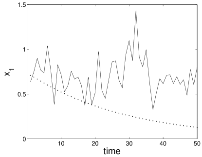
Figure 1: Example of fluctuations in a linear system

Fluctuations in a stochastic system are studied by way of the system’s moments Gardiner . The $p$th moment of a multivariate system is simply the expected value of $|\mathbf{x}|^{p}$; large moments, especially the low order moments such as the second and third, indicate that a system attains large values with non-negligible probability Rice . For example, the system of figure 1 has a divergent moments for $p\geq 3$.

Multiplicative noise causes fluctuations because its effect is to cause the moments of a system to diverge, even when the system converges in mean Redner ; LewontinCohen . In particular, divergent low-order moments in the neighborhood of a stable fixed point are likely to cause the large fluctuations described above. The evolution of the moments is thus an important consideration in regards to fixed point stability in systems whose interactions are subject to noise.

The asymptotic behavior of a random system and its moments is characterized by the system’s Lyapunov exponent and moment Lyapunov exponents Arnold1986 . Calculation of Lyapunov exponents for multivariate systems is very difficult in general, even in simple cases Tsitsiklis . Stability analysis and calculation of Lyapunov exponents for discrete linear stochastic systems and random matrix products has been a major area of research in mathematics BougerolLacroix ; Stewartmatrixpowers ; CohenNewman ; Gurvits ; Barabanov ; Hinrichsenpencils ; Hinrichsenpositive , control theory KumarVaraiya ; Xiao ; Moustakidis ; MiliVerriest , physics CrisantiPaladin ; VanKampen , engineering mechanics MaCaughey ; Kozin ; Haddad , and biology stabilityofecosystems ; LewontinCohen , among others. However, the subject of most research has been stability in mean, not stability of the moments. The traditional approach to determining convergence in random systems is to use bounds (above mathematics references; see also Khas1966 ; Mao , for example, for continuous systems).

There has been little previous work on calculating exact expressions for moment evolution in multidimensional stochastic systems. One exception is Arnoldperturbation for continuous 2-dimensional systems, the results of which are discussed in context in §7.

1.2 Problem statement and notation

We are studying a system evolving according to the difference equation

$$\mathbf{x}^{t}=(\mathbf{A}+\mathbf{B}^{t})\mathbf{x}^{t-1},$$ (2)

or

$$\mathbf{x}^{t}=[\prod_{\tau=1}^{t}(\mathbf{A}+\mathbf{B}^{\tau})]\mathbf{x}^{0}.$$ (3)

Here $\mathbf{x}$ is the system state, a vector of random variables and $\mathbf{B}^{t}$ is a matrix of white noise processes with mean 0. (That is, $\langle B^{t}_{ij}\rangle=0$ and $\langle B^{t}_{ij}B^{t^{\prime}}_{ij}\rangle\sim\delta_{tt^{\prime}}$.) The initial state $\mathbf{x}^{0}$ of the system is assumed to be fixed. The eigenvalues of the matrix $\mathbf{A}$ are $\lambda_{i}$; the largest eigenvalue $\lambda_{1}$ or simply $\lambda$ is simple and dominant, that is, $\lambda>\lambda_{i}$ for all $i\neq 1$.

The system size is $n$. We define the mean of the $\mathbf{A}_{ij}$ to be $a$, and the variance to be $\sigma_{A}^{2}$. In the mean value approximation, $\mathbf{A}\approx a\mathbf{G}$ where $\mathbf{G}$ is the matrix whose elements are all 1. We will be diagonalizing $\mathbf{A}$ into the form $\mathbf{P}\mathbf{\Lambda}\mathbf{P}^{-1}$, where $\mathbf{\Lambda}$ is the diagonal matrix of eigenvalues of $\mathbf{A}$, and

$$\mathbf{u} = \mathbf{P}_{i1}=\mbox{normalized right eigenvector}$$

$$~{}~{}~{}~{}~{}~{}~{}~{}~{}~{}~{}~{}~{}\mbox{corresponding to }\lambda;$$

$$\mathbf{v} = (\mathbf{P}_{1i}^{-1})^{T}=\mbox{non-normalized left eigenvector}$$

$$~{}~{}~{}~{}~{}~{}~{}~{}~{}~{}~{}~{}~{}~{}~{}~{}~{}\mbox{corresponding to }\lambda.$$

so that $|\mathbf{u}|=1$. Note that $\mathbf{v}\cdot\mathbf{u}=1$ and so $|\mathbf{v}|\geq 1$.

A vector $\mathbf{x}^{t}$ converges in mean if $\langle x^{t}_{i}\rangle$ converges for all $i$ . We use any typical definition for convergence. The system’s fixed point is stable whenever the system converges in mean, because the initial state is irrelevant to convergence Strang .

We define the pth moment of the system to be $\langle|\mathbf{x}^{t}|^{p}\rangle$. Moment convergence can be elegantly expressed in terms of moment Lyapunov exponents, discussed in Arnold1986 and defined as

$$L_{p}=\lim_{t\rightarrow\infty}\frac{\log\langle|\mathbf{x}^{t}|^{p}\rangle}{t}.$$ (6)

The asymptotic behavior of the $p$th moment is then given by $\langle|\mathbf{x}^{t}|^{p}\rangle\sim e^{tL_{p}}$ and the $p$th moment converges if

$$L_{p}\leq 0.$$

Finally, in the case that all the elements of the noise matrix have the same variance $b^{2}$, we define the critical value $b_{c}^{2}$ to be the level of noise above which the second moment diverges.

1.3 Overview of results

The central results of this paper are the approximations and exact expressions describing the evolution of moments of the system (2), in particular the second moment. The small noise case is treated first using a perturbation approach. This approach allows us to calculate the system’s approximate asymptotic distribution and moment Lyapunov exponents. For larger noises, an iteration technique is presented which gives both small and large noise results for the second moment. For certain types of noise, the iteration method allows us to calculate the second moment Lyapunov exponent exactly in any system. These results appear to be the first general analytic results for the Lyapunov exponents of discrete multivariate systems.

The analysis of this paper is valid in discrete systems with a simple, dominant eigenvalue. The eigenvalue requirement is satisfied by all nonnegative systems (see appendix B) and many arbitrary systems. Nonnegative BermanNeumann and positive FarinaRinaldi ; positivesystems discrete systems arise in Markov models, and the fields of biology, population models, economics (input-output models), finance, and cooperative problem solving, among others. Applications to arbitrary systems are too numerous to list.

Particular results of this paper are as follows. First, we show that in the small noise regime, the problem of approximating the asymptotic probability distribution of a multidimensional system reduces to the scalar case, which is trivial (§2.2, §4.1, §4.3). We thus obtain the expression

$$\langle|\mathbf{x}^{t}|^{p}\rangle=|\langle\mathbf{x}^{t}\rangle|^{p}e^{t\varepsilon^{2}\frac{p(p-1)}{2}+O(\varepsilon^{4})}$$ (7)

where $\langle\mathbf{x}^{t}\rangle$ is the expected (unperturbed) value of the system at time $t$, and $\varepsilon$ is a small parameter which depends on the noise and is calculated for various forms of noise (equation (29) and table 3). This approximation is justified by simulation (figures 6,7,8) and its accuracy is discussed briefly in §4.5.

In the case of larger noise, the iteration approach of section §5 presents a methodology for calculating the second moment Lyapunov exponent to any degree of accuracy in any system, provided the noise elements have the same variance. The exact value of the Lyapunov exponent is expressed as the largest eigenvalue of a matrix and its accuracy is justified in the simulation of figure 9.

It is shown that the results of the iteration technique agree with (7) for small noise, and with the $\lambda\rightarrow 0$ limit for large noise. It is also shown that all results agree with the trivial scalar case discussed in §2.2.

While the unperturbed value of the system depends only on the initial state and the dominant eigenvalue in the asymptotic limit, the moments depends on other properties of the system including the system size and the form of the noise. It is shown that

• the effect of a given level of noise can be magnified, in some cases greatly, if the dominant eigenvalue of the unperturbed system is ill-conditioned (§3, §4.3);

• the destabilizing effect of the noise is damped as the number of independent components of noise increases (“destructive interference” of independent noises) (§4.4, figure 7);

• the destructive interference of independent noises is maximized in the mean value limit (§1.2) and is mitigated by any deviation from this limit (§4.4, figure 8).

• large noise (§6.2), or small noise in systems with a very ill-conditioned dominant eigenvalue (§5.2, figure 9), almost certainly destabilizes the system.

We also present a discussion of the critical value for the noise variance above which the second moment diverges and fluctuations become a major consideration. This discussion is largely restricted to the case in which all the noise elements have the same variance for simplicity. We obtain the following expression for the critical value:

$$b_{c}^{2}=\frac{1}{n^{k}+\frac{f_{v}f_{u}\lambda^{2}}{1-\lambda^{2}}},$$ (8)

where $f_{u}$ and $f_{v}$ are parameters related to $\mathbf{A}$ and the type of noise considered which are very close to 1 in the large majority of systems, and $k$ equals 1 if all the noise elements are independent and 2 if they are all correlated. This expression is shown to be accurate in both the small and large noise cases, and is used to create a stability diagram for the system in figures 11 and 12.

The dependence of the critical value on system parameters is discussed. We show that

• for small noise, the critical value depends weakly on the system size and type of noise considered (§6.4, figure 13);

• for large noise, the critical value depends strongly on the system size and type of noise (§6.4);

• the critical value provides a much more accurate indication of the level of noise below which the second moment converges than a simple bound on convergence (§6.5, appendix D);

• for most convergent systems subject to small noise, the low-order moments diverge only if the unperturbed system converges slowly (§6.1).

This last statement is especially true for positive systems (figure 5); note that systems with slow convergence may have other problems besides fluctuations due to noise, such as large transient behaviorTrefethen .

Finally, we consider the continuous limit and show that our results only extend to this limit in certain very special cases (§7.1, §7.2).

1.4 Paper organization

The paper is organized as follows. In §2 we present simple preliminary results: asymptotic expressions for the system’s expected value, moments in the scalar ($n=1$) case, and second moment in the case that $\mathbf{A}=0$. Section 3 discusses the important properties of the multivariate system. Moment evolution is calculated for multivariate systems in the small noise limit using a perturbation approach in §4, and the result is discussed. Section 5 uses an iteration approach to treat the second moment’s evolution in the case of larger noise. The critical value of noise for second moment divergence is the subject of §6. The accuracy of the approximations is justified in numerical simulations throughout the paper. Finally, §7 presents a discussion of the continuous time limit.

2 Preliminaries

This section presents a calculation of the expected value of the system, as well as calculations of two limiting cases: a scalar stochastic system, and a multivariate system with no fixed part (noise only).

A discussion of the expected value of the system and its convergence properties is a necessary preliminary step to any study of the moments. The computation is trivial, as we show, because the noise is white with mean zero.

Calculation of the moments of a scalar system provides a framework which we will apply in the small noise limit of the multivariate case (§4). The scalar system also provides a demonstration of how multiplicative noise leads to a log-normal distribution and moment divergence.

The noise only, $\mathbf{A}=\mathbf{0}$ multivariate system is a system in which the moments can be found exactly, yielding the zeroth order term for the large-noise limit (see §5.3). The calculations involved also provide a useful preview of those in §5.

All of the calculations in this section are quite straightforward and have very likely been presented, in whole or part, in some previous work. However, we did not find a specific reference with the exception of MiliVerriest for a cursory treatment of the scalar case.

2.1 Expected value and unperturbed system

The expected (average) state of the system and the state of the unperturbed system are equivalent since the noise is white with mean 0. White noise means that $\mathbf{x}^{t-1}$ and $\mathbf{B}^{t}$ are independent, so that

$$\langle\mathbf{x}^{t}\rangle=(\mathbf{A}+\langle\mathbf{B}^{t}\rangle)\langle\mathbf{x}^{t-1}\rangle=\mathbf{A}\langle\mathbf{x}^{t-1}\rangle,$$

since the mean is 0. Thus

$$\langle\mathbf{x}^{t}\rangle=\mathbf{A}^{t}\mathbf{x}^{0}=\mathbf{x}^{t}_{\textnormal{unperturbed}}.$$

In systems with a simple dominant eigenvalue $\lambda$, the asymptotic behavior of unperturbed system is completely determined by the largest eigenvalue of $\mathbf{A}$Strang . For large $t$,

$$\mathbf{x}_{\textnormal{unperturbed}}^{t}=\lambda^{t}(\mathbf{v}\cdot\mathbf{x}^{0})\mathbf{u}$$ (9)

and the moment Lyapunov exponents are simply

$$L_{p}^{0}=p\log\lambda.$$ (10)

The system will converge to 0 for any initial conditions if $\lambda<1$, and it will diverge if $\lambda_{1}>1$. In the case of stochastic matrices with $\lambda=1$, the above formula is accurate because $\lambda$ is simple. We are not interested in the case in which $\mathbf{x}^{0}$ is orthogonal to $\mathbf{v}$.

2.2 Scalar stochastic system

In the case $n=1$ it is not difficult to determine the asymptotic distribution, as well as the exact expressions for any moment. We go through a derivation here because this analysis will apply to the small noise multivariate case. The scalar system is

$$x_{t}=x_{0}\prod_{\tau=1}^{t}(a+b_{\tau}),$$

where $\langle b_{\tau}\rangle=0$ and $\langle b_{\tau}b_{\tau^{\prime}}\rangle=b^{2}\delta_{\tau\tau^{\prime}}$. Notice that we express time as a subscript in this section, whereas in the multidimensional treatment time is a superscript.

2.2.1 Exact expressions

We have

$$\langle x^{p}_{t}\rangle = x_{0}^{p}\langle[a+b_{\tau}]^{p}\rangle^{t}$$ (11)

$$= x_{0}^{p}a^{pt}\left(\sum_{k=1}^{p}{p\choose k}\langle b_{\tau}/a\rangle^{k}\right)^{t}.$$

In particular, $\langle x_{t}\rangle=a^{t}$ and $\langle x^{2}_{t}\rangle=(a^{2}+b^{2})^{t}$, so that

$$L_{2}=\log(a^{2}+b^{2}).$$ (12)

2.2.2 Approximate asymptotic distribution

In this subsection we assume small noise, that is, $|b_{\tau}/a|<1$. This allows us to take logs and ensures that the moments of $b_{\tau}/a$ are well behaved. We have

$$\log\frac{x_{t}}{x_{0}}=t\log a+\sum_{\tau}s_{\tau}$$

where

$$s_{\tau}=\log(1+b_{\tau}/a).$$

The $s_{\tau}$ are i.i.d., so the sum is normal for large $t$ with mean $t\mu_{s}$ and variance $t\sigma_{s}^{2}$, where $\mu_{s}$ and $\sigma_{s}^{2}$ are the mean and variance of the $s_{\tau}$, by the central limit theorem. The system is thus log-normally distributed in the asymptotic limit and its moments are given by

$$\langle x_{t}^{p}\rangle=x_{0}^{p}a^{pt}e^{pt\mu_{s}+p^{2}t\sigma_{s}^{2}/2}.$$ (13)

Since we know that the first moment $\langle x_{t}\rangle=x_{0}a^{t}$ is independent of the noise, we can conclude that $\mu_{s}=-\sigma_{s}^{2}/2$ and we have

$$\langle x^{p}_{t}\rangle=\langle x_{t}\rangle^{p}e^{-t\mu_{s}p(p-1)}$$ (14)

in the large $t$ limit. Thus the Lyapunov exponents are given by

$$L_{p}=p\log a-\mu_{s}p(p-1),$$

or

$$L_{p}=L^{0}_{p}-\mu_{s}p(p-1)$$ (15)

where $L^{0}_{p}$ is the Lyapunov exponent for the unperturbed system. Notice that $\mu_{s}<0$ because the log function weights the negative values of $b_{t}/a$ more heavily than the positive ones.

Expanding the log in the expression for $\mu_{s}=\langle\log(1+b_{\tau}/a)\rangle$ we find:

$$\mu_{s}=-\sum_{k}\frac{\langle b_{\tau}/a\rangle^{k}}{k}(-1)^{k}.$$

The $\langle b_{\tau}/a\rangle^{k}$ term in the expansion must be $O(b/a)^{k}$ or smaller since $b_{\tau}/a$ can never exceed 1. Thus

$$L_{p}=L^{0}_{p}+p(p-1)(b/a)^{2}/2+O(b/a)^{3}.$$ (16)

The error is $O(b/a)^{4}$ if the noise is symmetric. In particular, for the second moment,

$$L_{2}\approx L^{0}_{p}+(b/a)^{2}+O(b/a)^{3},$$ (17)

in agreement with the exact value to second order.

The approximation and exact results for a scalar system are compared to simulation in figure 2 below. This system converges in mean but has diverging moments for $p\geq 3$. The parameters for the simulation are $a=0.97$ and normal noise with $b^{2}=0.05$. The solid lines show the average of the moments $\langle x_{t}^{p}\rangle$ for $p=1,2,3$ and 4, over $10^{6}$ runs. The dashed lines are the exact prediction (11) and are shown only for $p=3$ and 4. The crosses are the approximation (16); the inaccuracy for $p=4$ is due to the expansion of the log. The initial value was $x_{0}=1$ and noises larger than $a$ were not allowed.

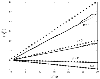
Figure 2: Moment evolution in scalar system

2.3 $\mathbf{A}=\mathbf{0}$ limit of multivariate case

Returning to the multivariate system, we consider as a first treatment the $\mathbf{A}=\mathbf{0}$ limit. The system’s evolution in this limit is given by

$$\mathbf{x}^{t}=\big{[}\prod_{\tau=1}^{t}\mathbf{B}^{\tau}\big{]}\mathbf{x}^{0}.$$ (18)

The expected value of $\mathbf{x}$ is $\mathbf{0}$. The expression for moments contains two or more occurrences of each $\mathbf{B}^{\tau}$; the difficulty in its evaluation, and in general the difficulty of any multivariate system, is that the noise matrices do not commute. However, when $\mathbf{A}=\mathbf{0}$ and the noise is white, the sum may be evaluated explicitly. Its value depends on the type of noise considered. In this section we show the details of how to evaluate such a sum; in later sections such steps will be skipped.

In principle any moment of $\mathbf{x}$ could be calculated exactly, given a particular distribution for the noise elements. Here we restrict our calculation to the second moment for clarity and simplicity.

2.3.1 Independent noises

We first consider the case where all the noise elements vary independently. The matrices $\mathbf{B}^{\tau}$ do not commute so we must consider the full term by term expansion to evaluate the second moment:

$$\langle|\mathbf{x}^{t}|^{2}\rangle = \sum_{i}\sum_{j_{1}j_{2}\ldots j_{t}}\sum_{k_{1}k_{2}\ldots k_{t}}\left\langle B^{1}_{j_{1}j_{2}}B^{2}_{j_{2}j_{3}}\cdot\ldots\right.$$

$$~{}~{}~{}~{}\left.\cdot B^{t}_{j_{t}i}x^{0}_{i}B^{1}_{k_{1}k_{2}}B^{2}_{k_{2}k_{3}}\cdot\ldots\cdot B^{t}_{k_{t}i}x^{0}_{i}\right\rangle$$

where the expected value goes inside the sum because it is a linear function. All the elements of every $\mathbf{B}$ are independent, and we get a $\delta_{j_{\tau}k_{\tau}}$ for every $\tau=1\ldots t$ when we sum on the $k$’s. This gives

$$\langle|\mathbf{x}^{t}|^{2}\rangle=\sum_{j_{1}j_{2}\ldots j_{t}i}\langle(B^{1}_{j_{1}j_{2}})^{2}\rangle\langle(B^{2}_{j_{2}j_{3}})^{2}\rangle\cdot\ldots\cdot\langle(B^{t}_{j_{t}i})^{2}(x^{0}_{i})^{2}\rangle$$ (20)

When all the noise elements have the same variance $b^{2}$, each of the $t$ sums on $j_{2},\ldots,j_{t}$ and $i$ simply gives a factor of $nb^{2}$. The remaining sum is just the norm squared of $x^{0}$, and we obtain

$$\langle|\mathbf{x}^{t}|^{2}\rangle=(nb^{2})^{t}|\mathbf{x}^{0}|^{2}.$$ (21)

If the noises did not all have the same variance, the result would be identical with $b^{2}$ replaced the average variance

$$\bar{b}^{2}=\frac{\sum_{ij}\langle(B_{ij})^{2}\rangle}{n^{2}}.$$

2.3.2 Correlated noises

When all the noises are correlated with the same variance (T noise) the calculation is similar except that both the sum on the $\{j_{\tau}\}$ and the sum on the $\{k_{\tau}\}$ in equation (20) give a factor of $n$. We thus obtain

$$\langle|\mathbf{x}^{t}|^{2}\rangle=(n^{2}b^{2})^{t}|\mathbf{x}^{0}|^{2}.$$ (22)

We note that this result can be also found immediately by transforming to the eigenspace, since in this case $\mathbf{B}$ is proportional to the matrix $\mathbf{G}$ of all ones which has $\lambda=n$ and all other eigenvalues equal to 0.

The case of noises where only certain elements are correlated provides an intermediate case between independent and correlated noises. The expressions are complex and are left for future work.

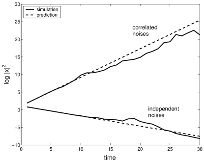
Figure 3: Second moment evolution for $\mathbf{A}=\mathbf{0}$

Second moment evolution in the noise-only case is shown in figure 3. The simulations show the value of $|\mathbf{x}|^{2}$ averaged over 1,000 runs, in the independent noise case, and 100,000 runs for correlated noise. Here $n=3$ and the elements of $\mathbf{B}$ were chosen from a normal distribution with variance 0.25. The simulations are compared to the predictions of (21) and (22).

3 Properties of multivariate stochastic systems

3.1 Log-normal character of distribution

As we saw in §2.2, scalar stochastic systems with stationary multiplicative noise are log-normally distributed with parameters proportional to time, so the system moments evolve as $\exp[tp(\mu+p\sigma^{2}/2)]$. While $\mu$ is typically negative, for large $p$ the positive $p\sigma^{2}/2$ term dominates and causes divergence. The effect of the multiplicative noise is thus to cause the system’s $p$th moments to diverge for all $p$ greater than some $p_{0}$.

While the components of multidimensional stochastic systems with multiplicative noise do not have an exact log-normal distribution, they retain the general log-normal character including the heavy tail and divergent moments. To be exact, any element of a product of $t$ stationary random matrices is asymptotically log-normally distributed with parameters proportional to $t$Bellman ; FurstenbergKesten . Components of a multivariate stochastic difference system are thus linear combinations of log-normal variables with parameters proportional to $t$. Just as in the scalar case, therefore, multiplicative noise in multivariate systems causes the system’s moments to diverge.

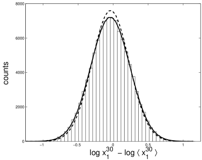
Figure 4: Approximately log-normal distribution of the system state

In the particular case of small noise and simple dominant $\lambda$, the distribution of the elements of a multivariate system is very close to log-normal. This is shown in the simulation of figure 4 which presents a histogram of the log of 100,000 instances of $x^{30}_{1}$ in a positive system whose $\mathbf{A}$ is given in (63). The data were normalized by the expected value $\langle\mathbf{x}^{30}_{1}\rangle$. The solid line is a Matlab normal fit with $\mu=-.0389$ and $\sigma=0.2725$. The dashed line is the prediction of §4.3 and has $\mu=-0.348$ and $\sigma=0.2639$.

3.2 Relevant properties of $\mathbf{A}$

3.2.1 Simple dominant eigenvalue

In this paper we only consider systems with simple, dominant $\lambda$. Geometrically, the effect of $\mathbf{A}$ repeatedly acting on a vector is to bring that vector into the direction of $\mathbf{u}$ and to multiply its length repeatedly by $\lambda$. The behavior of unperturbed multivariate systems with a simple, dominant $\lambda$ is thus equivalent to scalar systems in the asymptotic limit.

The requirement that $\lambda$ be simple and dominant is met in all nonnegative systems of interest (appendix B), so our treatment of nonnegative systems is comprehensive. Although many arbitrary systems meet this condition as well, some do not and we do not attempt to treat these cases. We also neglect systems with defective (non-diagonalizable) $\mathbf{A}$, which form a set of measure 0, because the nonzero elements of $\mathbf{A}$ are impossible to determine exactly in most applications.

3.2.2 Condition of $\mathbf{\lambda}$

The effect of noise on a multivariate system, from a geometric perspective, is to perturb both the direction and length of the vector $\mathbf{x}$. Noise as a small perturbation means that a given noise matrix does not swing the $\mathbf{x}$ far from the direction of $\mathbf{u}$ or multiply $|\mathbf{x}|$ by a factor far from $\lambda$. In this regime, the dynamics are well approximated by the dynamics of a perturbed scalar system.

The regime of small noise, for the multivariate systems, is determined not only by the size of the noise elements but also by the sensitivity of the system to perturbation. There exist matrices whose eigenvalues and eigenvectors are violently affected by even a small perturbation to the matrix elementsGolubbook ; Edelman . For a perturbation treatment, we need to know how much the dominant eigenvalue $\lambda$ and its eigenvector $\mathbf{u}$ of the system are perturbed by a given level of noise.

The response of $\lambda$ to noise is characterized by a quantity $\kappa(\lambda)$ called the condition of $\lambda$. When $\kappa(\lambda)$ is large $\lambda$ is said to be ill-conditioned, meaning that its response to a system perturbation is large with respect to the perturbation. Even a small noise causes moment divergence in systems with an ill-conditioned $\lambda$. Conversely, when $\kappa(\lambda)=1$, $\lambda$ is said to be perfectly conditioned; its response to a system perturbation is the smallest possible and is on the order of the size of the perturbation. In systems with a well-conditioned $\lambda$, the perturbation approximation is applicable to relatively large noises.

The change in $\lambda$ due to a small noise matrix $\mathbf{B}$ (small in the sense that
$|\mathbf{B}|=\delta\ll 1$) is given by

$$\delta\lambda\approx\mathbf{v}\cdot(\mathbf{B}\mathbf{u})$$ (23)

to first order in $\delta$. Taking norms, we obtain the expression for the condition of $\lambda$ in the case of normalized $\mathbf{u}$:

$$\kappa(\lambda)=|\mathbf{v}|.$$ (24)

It is clear that $\kappa\geq 1$ by the Schwartz inequality. The sensitivity of $\mathbf{u}$ to noise may also be calculated to first orderGolubbook and depends on the condition of $\lambda$. It also depends on the gaps $\lambda-\lambda_{i}$ between the dominant eigenvalue and the others, and is therefore related to the accuracy of the approximation

$$\mathbf{A}^{p}\approx\lambda^{p}\mathbf{u}\mathbf{v}^{T}$$ (25)

obtained by neglecting all $\lambda_{i}^{p}$ compared to $\lambda^{p}$. In the limit that $\lambda_{2}\rightarrow 0$, 25 is exact for all $p$ and the sensitivity of $\mathbf{u}$ is minimized.

The level of noise which qualifies as a small perturbation must therefore depend on $\kappa(\lambda)$ and $\lambda-|\lambda_{2}|$, which it does, as we will show. The effect of a given level of noise is the smallest in well-behaved systems with a well-behaved $\lambda$ and small eigenvalue gap.

Matrix type	Eigenvalue gap	Condition $\kappa(\lambda)$
	$\lambda-|\lambda_{2}|$	of $\lambda$
$\mathbf{A}=a\mathbf{G}$	0	1
small $\sigma_{A}^{2}$	small	close to 1
normal $\mathbf{A}$	?	1
large $\sigma_{A}^{2}$	possibly small	possibly large

Table 1: Properties of some types of $\mathbf{A}$. Recall that $\mathbf{G}$ is the matrix of all 1’s (mean value approximation).

It is difficult to generally characterize the condition of $\lambda$ and the eigenvalue gap in terms of more physical properties of the matrix $\mathbf{A}$. What we can say is summarized in Table 1.

Systems close to the mean value approximation (recall $\mathbf{A}\approx a\mathbf{G}$ where $\mathbf{G}$ is a matrix of 1’s in the mean value approximation; §1.2) are sure to be well-behaved; however, some systems far from the mean value approximation are also well-behaved, as shown in figure 5 below as well as figures 15 and 14.

The correlation between eigenvalue gap and condition number of $\lambda$ are demonstrated in the scatter plots of figure 5 which show the eigenvalue gap versus $\kappa(\lambda)$ for 10000 randomly generated $5\times 5$ matrices. The matrices were generated from a normal distribution (top left), uniform distribution (top right), uniform distribution with probability 1/2 and 0 with probability 1/2 (bottom left) and uniform distribution with mean 0.2 and variance 0.02 (bottom right). For the arbitrary matrices, only those with real $\lambda$ were accepted and the entries were normalized so that $\lambda=1$. Note the difference in the regions plotted.

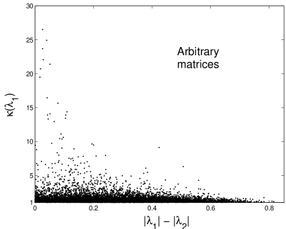
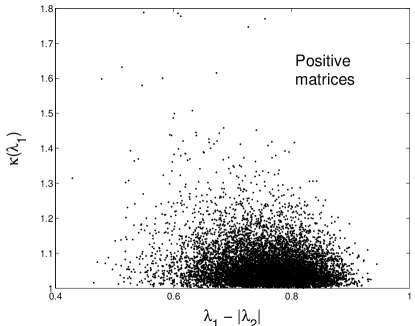
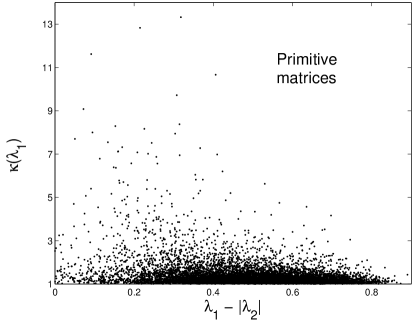
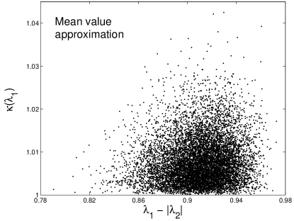
Figure 5: Eigenvalue gap versus condition of $\lambda$ in randomly generated matrices.

As shown in the figure, the likelihood that a given system is well-behaved is larger for nonnegative matrices than for arbitrary matrices, and larger still for positive matrices. See appendix C for further discussion.

3.2.3 Limits on average element size

Finally we note that in the case of nonnegative matrices, it is impossible to have a small $\lambda$ if the elements of $\mathbf{A}$ are too large. Many quite accurate bounds on the largest eigenvalue of nonnegative matrices exist (see Minc for a list); a relatively inaccurate but analytically tractable bound is the row sum bound, $\min_{i}(\sum_{j}A_{ij})\leq\lambda\leq\max_{i}(\sum_{j}A_{ij})$. This estimate implies that on average we need to take

$$a<1/n$$ (26)

to keep $\lambda<1$ and ensure that the system converges in mean. This is exactly the asymptotic $n$ result of Juhasz , and the result we would obtain in the mean value approximation $\mathbf{A}\approx a\mathbf{G}$.

3.3 Types of noise for multivariate systems

For multivariate systems many different forms of noise are possible, distinguished by whether the elements are correlated and how large their relative variances are. In this paper we consider five cases which are analytically tractable and have some relevance to physical systems. The correlation rules for these cases are shown in table 2 which provides a summary.

For the correlation we consider three cases. Uncorrelated noise means that the elements of the noise matrix vary independently. Totally correlated noise means that all the noise elements vary in the same way at each time step. For symmetric systems, we consider symmetrically correlated noise.

For the variance we consider two possibilities. For homogeneous noise, the variance of every element is identical and equal to $b^{2}$. For proportional noise, the standard deviation of $B_{ij}$ is proportional to $A_{ij}$ by some factor $q$ which we will take to be less than 1.

Noise type	Correlation rule
Uncorrelated homogeneous (UH)	$\langle B_{ij}B_{i^{\prime}j^{\prime}}\rangle=b^{2}\delta_{ii^{\prime}}\delta_{jj^{\prime}}$
Symmetrically correlated homogeneous (SH)	$\langle B_{ij}B_{i^{\prime}j^{\prime}}\rangle=b^{2}(\delta_{ii^{\prime}}\delta_{jj^{\prime}}+\delta_{ij^{\prime}}\delta_{i^{\prime}j})$
Totally correlated (T)	$\langle B_{ij}B_{i^{\prime}j^{\prime}}\rangle=b^{2}$
Uncorrelated proportional (UP)	$\langle B_{ij}B_{i^{\prime}j^{\prime}}\rangle=q^{2}(A_{ij})^{2}\delta_{ii^{\prime}}\delta_{jj^{\prime}}$
Symmetrically correlated proportional (SP)	$\langle B_{ij}B_{i^{\prime}j^{\prime}}\rangle=q^{2}(A_{ij})^{2}(\delta_{ii^{\prime}}\delta_{jj^{\prime}}+\delta_{ij^{\prime}}\delta_{i^{\prime}j})$

Table 2: Correlation rules for types of noise considered in this paper

4 Small noise as a perturbation

In this section we determine approximate expressions for the moment Lyapunov exponents for multivariate systems subject to small noise using a perturbation treatment. We examine the dependence of the Lyapunov exponents on system properties, and discuss the accuracy of the approximation.

First let us reexpress the matrix product in (3):

$$\mathbf{x}^{t} = \left[\prod_{\tau=1}^{t}(\mathbf{A}+\mathbf{B}^{\tau})\right]\mathbf{x}^{0}$$

$$= \left[\sum_{\mathbf{Y}^{t}=\mathbf{A},\mathbf{B}^{t}}\sum_{\mathbf{Y}^{t-1}=\mathbf{A},\mathbf{B}^{t-1}}\sum_{\mathbf{Y}^{1}=\mathbf{A},\mathbf{B}^{1}}\mathbf{Y}^{t}\mathbf{Y}^{t-1}\cdots\mathbf{Y}^{1}\right]\mathbf{x}^{0}$$

$$= \sum_{\textnormal{each }\mathbf{Y}^{\tau}=\mathbf{A},\mathbf{B}^{\tau}}\mathbf{Y}^{t}\mathbf{Y}^{t-1}\cdots\mathbf{Y}^{1}\mathbf{x}^{0}$$ (28)

meaning that each $\mathbf{Y}^{\tau}$ in the sum can be either $\mathbf{A}$ or $\mathbf{B}^{\tau}$, for $\tau=1\ldots t$. There are $2^{t}$ terms in the sum; each term is a vector.

4.1 Perturbation expansion

The perturbation expansion consists of considering only terms in (28) which have very few $\mathbf{B}$’s. For small noise, these terms make the only important contribution to the sum. Let us assume that this is so without justification, even before we define small noise.

The reason that this strategy simplifies the calculation is as follows. Consider the evolution in time of the length and direction of a single term of (28) with few $\mathbf{B}$’s. In the asymptotic limit, a typical term with few $\mathbf{B}$’s has long strings of consecutive $\mathbf{A}$’s broken by single occurrences of $\mathbf{B}$’s. As far as the direction of such a term, the long strings of $\mathbf{A}$’s act to bring it parallel to $\mathbf{u}$ as previously mentioned (see (25)). When a $\mathbf{B}^{\tau}$ acts on the term, the term lies almost parallel to $\mathbf{u}$; even though the noise causes the term to point away from $\mathbf{u}$, the next string of $\mathbf{A}$’s brings it back to the direction of $\mathbf{u}$ before another noise term occurs. The action of $\mathbf{B}^{\tau}$ is thus independent of $\tau$. As to the length, a string of $p$ $\mathbf{A}$’s simply multiplies the term length by $\lambda^{p}$; and the $\mathbf{B}$’s multiply the length by some stationary random variable.

In a term with few $\mathbf{B}$’s, therefore, the position of the matrices in the sum (28) is unrelated to their net effect on the term. Thus the matrices in the sum can be replaced by scalars, and the matrix product (4) becomes a product of scalars. To illustrate this, consider a typical term for $t=10$ with a $\mathbf{B}^{\tau}$ only in the $\tau=6$ spot:

$$\mathbf{A}\mathbf{A}\mathbf{A}\mathbf{A}\mathbf{B}^{6}\mathbf{A}\mathbf{A}\mathbf{A}\mathbf{A}\mathbf{A}\mathbf{x}^{0} \approx (\lambda^{4}\mathbf{u}\mathbf{v}^{T})(\mathbf{B}^{6})(\lambda^{5}\mathbf{u}\mathbf{v}^{T})\mathbf{x}^{0}$$

$$\approx \lambda^{10}\varepsilon_{6}\mathbf{u}(\mathbf{v}\cdot\mathbf{x}^{0})$$

where we define the random variable

$$\varepsilon_{\tau}=\frac{\mathbf{v}^{T}\mathbf{B}^{\tau}\mathbf{u}}{\lambda}.$$ (29)

In general, a term of the sum (28) that has long strings of $\mathbf{A}$’s and $m$ isolated $\mathbf{B}$’s $\{\mathbf{B}^{\tau_{1}},\ldots,\mathbf{B}^{\tau_{m}}\}$ points in the direction of $\mathbf{u}$ and has length $\lambda^{t}(\varepsilon_{\tau_{1}}\cdot\ldots\cdot\varepsilon_{\tau_{m}})\mathbf{u}(\mathbf{v}\cdot\mathbf{x}^{0})$. Such terms dominate the sum (28) (see §4.5) and so the system state is given approximately by

$$\mathbf{x}^{t}\approx\mathbf{u}(\mathbf{v}\cdot\mathbf{x}^{0})\lambda^{t}\prod_{\tau=1}^{t}(1+\varepsilon_{\tau}).$$ (30)

The random variables $\varepsilon_{\tau}$ are i.i.d. and satisfy $\langle\varepsilon_{\tau}\rangle=0$; the moments depend on the form of the noise. Notice that the numerator of $\varepsilon_{\tau}$ is exactly equal to the first order change in $\lambda$ due to a small perturbation to $\mathbf{A}$ (23) and thus closely related to the condition $\kappa(\lambda)$ (24). The eigenvalue gap and thus the sensitivity of $\mathbf{u}$ is implicitly involved in this expression from the application of (25).

4.2 Criterion for small noise

The simplest small noise criterion is

$$\langle\varepsilon_{\tau}^{p}\rangle\ll 1$$

for all $p$. This is a rather complicated condition since the calculation of all the moments can be difficult for some forms of noise. Instead we choose a more restrictive (triple) condition,

$$P(|\varepsilon_{\tau}|>1) = 0$$

$$\langle\varepsilon_{\tau}^{p}\rangle \sim \varepsilon^{p^{\prime}},\ \ p^{\prime}\leq p$$ (31)

$$\varepsilon^{2} \ll 1$$ (32)

Note that this requirement is not trivial as in the scalar case because the condition of $\lambda$ can be large. Less restrictive conditions are possible but this will enable us to better understand the dynamics by taking logs and expanding in a power series in $\varepsilon$.

4.3 Moment evolution

Using the perturbation expansion of section 4, we may now present approximate expressions for the moments of a multivariate stochastic system. We do so by calculating the approximate Lyapunov exponents, proceeding from (30) exactly as in the scalar case of §2.2.2 with $\varepsilon_{\tau}$ playing the role of $b_{\tau}$ and $\lambda$ the multidimensional analog of $a$.

We thus find

$$L_{p} \approx p\log\lambda-p(p-1)\langle\ln(1+\varepsilon_{\tau})\rangle$$ (33)

$$\approx L^{0}_{p}+p(p-1)\frac{\varepsilon^{2}}{2}+O(\varepsilon^{3})$$

where

$$L^{0}_{p}=p\log\lambda$$

is the Lyapunov exponent for the unperturbed system and the error is $O(\varepsilon^{4})$ if the noise is symmetric. The system moments are

$$\langle|\mathbf{x}^{t}|^{p}\rangle \approx |\mathbf{v}\cdot\mathbf{x}^{0}|^{p}e^{tL_{p}}$$ (34)

$$\approx |\langle\mathbf{x}^{t}\rangle|^{p}e^{t\varepsilon^{2}\frac{p(p-1)}{2}+O(\varepsilon^{3})}.$$

In particular,

$$L_{2}\approx L^{0}_{2}+\varepsilon^{2}$$ (35)

to second degree in $\varepsilon$, and

$$\langle|\mathbf{x}^{t}|^{2}\rangle\approx|\langle\mathbf{x}^{t}\rangle|^{2}e^{t\varepsilon^{2}}.$$ (36)

Notice that to this level of approximation, first moment (norm) convergence is not distinguishable from convergence in mean.

Noise Type	$\varepsilon^{2}$
UH	$\frac{v^{2}b^{2}}{\lambda^{2}}$
SH	$\frac{2b^{2}}{\lambda^{2}}$
T	$\frac{b^{2}}{\lambda^{2}}(\Sigma_{i}v_{i})^{2}(\Sigma_{i}u_{i})^{2}$
UP	$\frac{fq^{2}}{\lambda^{2}}\sum_{ij}v^{2}_{i}(A_{ij})^{2}u_{j}^{2}$
SP	$\frac{fq^{2}}{\lambda^{2}}\sum_{ij}(A_{ij})^{2}[v_{i}^{2}u_{j}^{2}+v_{i}v_{j}u_{i}u_{j}]$

Table 3: Values of $\varepsilon^{2}$ for the types of noise defined in §3.3

To proceed beyond these expressions we must evaluate $\varepsilon^{2}=\langle(\frac{\mathbf{v}^{T}\mathbf{B}\mathbf{u}}{\lambda})^{2}\rangle$, which we cannot do without specifying the form of the noise. The values of $\varepsilon^{2}$ for the noises described in §3.3 are easily calculated and presented in table 3. Here UP is uncorrelated proportional noise, UH is uncorrelated homogeneous, SP is symmetrically correlated proportional, SH is symmetrically correlated homogeneous, and T is and totally correlated. In the proportional noise, $f$ is a factor which depends on the distribution chosen; for example, $f=1$ for normal noise and $f=1/3$ for uniform noise. In the case of symmetrically correlated noise, a symmetric $\mathbf{A}$ is assumed.

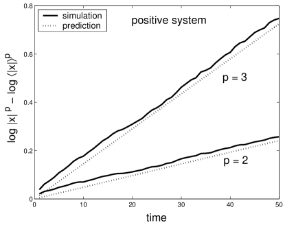
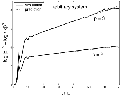
Figure 6: Moment evolution in two systems

The accuracy of the above approximations for the moment evolution is demonstrated in figure 6. In this figure, the log of the 2nd and 3rd moments of two randomly generated systems are shown. The plots are normalized by the expected value (unperturbed value) of the system and show only the noise part. The solid line is the average over 10,000 runs of the simulation, and the dotted line shows the analytic prediction of (34). At left is the positive system of (63) subjected to uniform UP noise with $q=0.5$. Note that the asymptotic limit is reached almost immediately in this system. At right is an arbitrary system with simple dominant $\lambda$ subjected to normal UH noise with $b=0.1$. This system has large transient behavior before it settles in to its asymptotic limit around $t=20$. The analytic prediction, which cannot account for the transient, has been artificially placed to demonstrate the asymptotic accuracy of the slope.

4.4 Dependence on system size

We can now explore the $n$ dependence of the moments. Because the small noise case is important for applications, we present a detailed discussion of the size dependence based only on the expressions developed thus far. A different discussion of the $n$ dependence for larger noises is presented in §6.4. For simplicity, we consider only the second moment in this section.

As we show, independently varying noises “interfere” with each other and diminish the effect of the noise, compared to the unperturbed system. Thus, the effect of the noise decreases as $n$ increases in the case of uncorrelated noise. There is no $n$ dependence to second order, however, in the case of totally correlated noise. Symmetrically correlated noise provides an intermediate case.

We also show that for noise proportional to the system elements, as the system deviates from the mean value approximation and in particular becomes closer to diagonal, the destructive interference is decreased and the noise has a greater effect.

4.4.1 Mean value approximation

As a first simplification, we consider the mean value approximation where $\mathbf{A}\approx a\mathbf{G}$. In this case, $v_{i}\approx u_{i}\approx 1/\sqrt{n}$ for all $i$, and $\lambda\approx na$. We consider homogeneous noise (all the noise elements have the same variance, which is almost equivalent to proportional noise in the mean value approximation) with variance $b^{2}=q^{2}a^{2}$, $q<1$.

Noise Type	$L_{2}$
UH	$L_{2}\approx L^{0}_{2}+\frac{q^{2}}{n^{2}}$
SH:	$L_{2}\approx L^{0}_{2}+\frac{q^{2}}{n^{2}/2}$
T:	$L_{2}\approx L^{0}_{2}+q^{2}$

Table 4: Approximate value of $L_{2}$ for three types of homogeneous noise

Using (35) and table 3, the values of $L_{2}$ for three types of homogeneous noise are easily computed in the mean value approximation and are shown in table 4. These expressions are to be compared to the scalar case $L_{2}\approx L^{0}_{2}+q^{2}$ (equation 17).

Note in particular how the noise effect (the $q^{2}$ term) is divided by a factor related to the number of independent elements of the noise. This destructive interference is not surprising when we consider why multiplicative noise processes generate the anomalously large events which make up the heavy tail of the log-normal distribution. The anomalous events result from a long sequence of large, positive noises 02thing . When there are $n^{2}$ independent noises per time step, as opposed to 1, anomalous events are rarer. However, when all the elements of noise vary identically, the effect of the noise is the same in scalar and multidimensional systems. Note that symmetric noise provides an intermediate calculable case; there are $n(n+1)/2$ independent components in a symmetric noise.

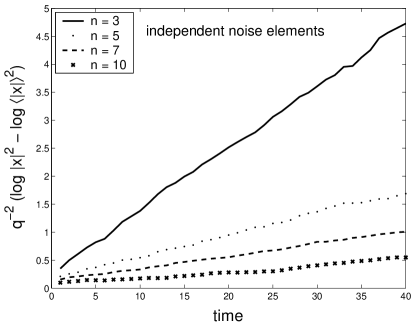
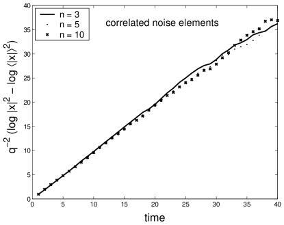
Figure 7: Dependence of the noise effect on the number of independent noise elements.

The dependence of the noise effect on the number of independent elements of the noise is demonstrated in the simulation of figure 7. By table 4 and equation (36)

$$\langle|\mathbf{x}|^{2}\rangle/|\langle\mathbf{x}\rangle|^{2}=e^{tfq^{2}}$$

in the asymptotic limit, where $f=1/n^{2}$ for UH noise (all noise elements independent) and $f=1$ for T noise (all noise elements correlated). Accordingly we plot
$q^{-2}(\log|\mathbf{x}|^{2}-\log|\langle\mathbf{x}\rangle|^{2})$, averaged over 100,000 runs, for various values of $n$. On the left is the plot for UH noise, where the lines should have slope $1/n^{2}$; on the right is the plot for T noise where the slope should be 1 for any $n$. The agreement is excellent. The $\mathbf{A}$’s for these systems were randomly generated from uniform distributions with small variance. The initial state was a vector of 1’s, and $q=1/4$. Because we are in the mean value approximation, $\lambda_{2}$ is very small for these systems and the asymptotic limit for $t$ begins almost immediately.

4.4.2 Deviation from the mean value approximation

We examine the effect of a deviation from the mean value approximation on $L_{2}$ in the case of uncorrelated proportional noise. The result is that the noise effect roughly increases the larger the deviation, as the $1/n^{2}$ damping caused by the independent noise elements is mitigated. This is because we have assumed that the typical size of a noise element is proportional to the corresponding element of $\mathbf{A}$ (UP noise), so that small entries of $\mathbf{A}$ contribute little to the interference effect of the independent noises.

In this subsection we assume that the approximation (25) is accurate for $p=2$ so that $A_{ij}^{2}\approx\lambda^{2}u_{i}^{2}v_{j}^{2}$. Recall that (25) is generally more accurate the closer $\mathbf{A}$ is to the mean value approximation, but it can be accurate even if the variance of the $A_{ij}$ is large, as discussed above.

With the above approximation we have

$$L_{2}\approx\ln\lambda^{2}+q^{2}w^{4}$$ (37)

where we define

$$w^{2}=\sum_{i}v^{2}_{i}u^{2}_{i}.$$

Comparing (37) to the mean value case, we see that the $1/n$ factor is replaced by $w^{2}$. This quantity satisfies

$$1/n\leq w^{2}\leq 1$$

since $\mathbf{v}\cdot\mathbf{u}=1$. The lower bound is achieved in the mean value case; the upper bound is achieved when $\mathbf{A}$ is diagonal. $w^{2}$ is thus a rough measure of the deviation of the $A_{ij}$ from the mean value approximation; it generally increases as the variance of the $A_{ij}$ increases.

Larger values of $w^{2}$ for deviations from the mean value approximation thus mean a larger noise effect. This effect is demonstrated in figure 8, which is analogous to figure 7 and compares the noise parts of the second moment $q^{-2}(\log|\mathbf{x}|^{2}-\log|\langle\mathbf{x}\rangle|^{2})$ of a mean value approximation (MVA) system and of a system with the same $\lambda$ and $n=5$ but whose elements have a much larger standard deviation. UP noise was considered, so the slope should be $w^{4}$ by (37). The dashed line system has $w^{2}=0.2888$, $w^{4}=0.0834$ while the MVA system has $w^{2}=0.2002\approx 1/n$ and $w^{4}=0.04$; a rough linear interpolation fit to the data shows an asymptotic slope 0.095 for the dashed system and 0.0385 for the MVA system. Note how the dashed system does not immediately reach its asymptotic limit; it has $|\lambda_{2}|\sim\lambda/2$ as opposed to $|\lambda_{2}|\ll 1$ for the MVA system.

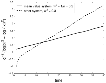
Figure 8: Larger noise effect of a deviation from the mean value approximation

4.4.3 Large $n$ limit and homogeneous noise

When the noise is homogeneous we can apply results on spectral theory of matrices to study the $n$ dependence in the large $n$ limit without appealing to a mean value approximation. In the case of a symmetric matrix with entries drawn from a distribution with mean $a$ and variance $\sigma^{2}_{a}$

$$\lambda=na+\sigma^{2}_{a}/a$$

on average FurediKomlos . For an arbitrary (asymmetric) matrix Juhasz

$$\lambda\sim na,$$

which is really just the mean value approximation.

Arbitrary system	$L_{2}\sim L^{0}_{2}+\frac{b^{2}/a^{2}}{n^{2}}$
Symmetric system	$L_{2}\sim L^{0}_{2}+\frac{b^{2}/a^{2}}{(n^{2}+2n\sigma_{a}^{2}/a^{2})/2}$

Table 5: Large $n$ dependence of arbitrary and symmetric systems with homogeneous noise.

We thus obtain table 5 for the $n$ dependence. Recall the notation $b^{2}$ for the variance of the homogeneous noise. Note again the $n^{2}$ damping in the arbitrary system, and a damping on the order of $n(n+1)/2$ in the symmetric case, in agreement with the previous analysis. We have assumed independently varying noise in the arbitrary system, and symmetrically varying noise in the symmetric system.

4.5 Approximation justification, accuracy, failure

The justification for equation (30) in the small noise approximation is as follows. Expand the product $\prod_{\tau}(1+\varepsilon_{\tau})$ into a sum. The typical size of the random variable $\varepsilon_{\tau}$ is $\varepsilon$, and the largest contribution to the sum comes from terms with $k_{\max}$ $\varepsilon_{\tau}$’s, where

$$k_{\max}=[t\varepsilon]$$

is the binomial expected value. The brackets denote the closest integer. This means that the largest terms in the sum come from terms of (28) with $k_{\max}$ $\mathbf{B}$’s. From symmetry considerations it is clear that in the asymptotic limit, the average separation $d$ between two $\mathbf{B}$’s in a term with $k_{\max}$ $\mathbf{B}$’s is

$$\langle d\rangle=\frac{t}{1+t\varepsilon},$$

which is large for small $\varepsilon$ and asymptotically independent of $t$. Furthermore, in a term with $k_{\max}\approx t\varepsilon$ $\mathbf{B}^{\prime}s$, the separation satisfiesRice

$$P(d<d_{0})=1-(1-\frac{d_{0}}{t})^{t\varepsilon}\rightarrow\varepsilon d_{0}\\$$

in the asymptotic limit, which is small for small $\varepsilon$ and independent of $t$. Therefore, the important terms of (28) for small $\varepsilon$ are those with a few $\mathbf{B}$’s separated by long strings of $\mathbf{A}$’s for all $t$ .

However, this analysis does not tell the entire story. The accuracy of the perturbation approximation is in fact much higher than one would expect from the above calculation. To understand this, consider a term of the sum (28) with many $\mathbf{B}$’s. This term’s direction is impossible to determine in general because each noise matrix transforms it arbitrarily. There are many such terms and they are all affected by a different set of noise matrices. Their directions are thus widely distributed in $\mathbf{R}^{n}$ and mostly cancel out in the sum.

When $\varepsilon$ is not small terms in the sum (28) with many $\mathbf{B}$’s become important. This causes the perturbation approximation to be inaccurate for two different reasons. First, when $\mathbf{B}$’s are adjacent, the approximation of replacing $\mathbf{B}$ by $\varepsilon_{\tau}$ is poor; second, when there are many strings of only a few adjacent $\mathbf{A}$’s, both replacing $\mathbf{A}$ by $\lambda^{2}$ and $\mathbf{B}^{\tau}$ by $\varepsilon_{\tau}$ can be inaccurate. The relative importance of these two inaccuracies can be different. For example, the accuracy of the $\mathbf{A}$ factor is independent of $n$ while the accuracy of the $\mathbf{B}$ factor decreases as $n$ increases.

It is difficult to determine a cut-off where $\varepsilon$ becomes large. The overall error may be much smaller than the error of each term of the sum (28), because the deviations of the terms may lie in different directions and cancel out in the sum. It is clear that the cut-off depends on how quickly $\mathbf{A}^{p}$ brings a random vector into alignment with $\mathbf{u}$, but even this is a complicated function of the eigenvalue gap and the condition of $\lambda$ Golubbook . To account for large $\varepsilon$ and handle the contribution from neighboring $\mathbf{B}$’s accurately for large $n$, we develop a different approximation in the next section.

5 Arbitrary noise using iteration approximation

We now present a different method, the iteration technique, which can be applied to find an approximate value for the second moment for small or large noise in well- or ill-conditioned systems.

For homogeneous noise (that is, all the noise elements having the same variance), the approximation can be extended to any level of accuracy for any noise. Unfortunately, for other forms of noise including proportional noise, only the first approximation is applicable.

In addition to providing a way to treat systems where the noise effect is not small, this technique is able to detect the explicit $n$-dependence of the noise effect. This effect is very slight in the small noise case, but quite important for larger noises.

The general strategy of the method is to express $\langle|\mathbf{x}^{t+1}|^{2}\rangle$ as a time-independent function of $\{\langle|\mathbf{x}^{t}|^{2}\rangle,\langle|\mathbf{x}^{t-1}|^{2}\rangle,\ldots\}$ in the asymptotic limit. A similar technique was independently developed in Roy for other applications.

5.1 First approximation

The first approximation of this method consists of applying the relation

$$\sum_{ij}(A^{r}_{ij})^{2}\approx\lambda^{2r}v^{2},$$ (38)

where $\mathbf{u}$ has been normalized to have length 1, for all $r$, even $r=1$. In this approximation we can express $\langle|\mathbf{x}^{t+1}|^{2}\rangle$ as a $t$-independent function of $\langle|\mathbf{x}^{t}|^{2}\rangle$ alone, as we will see. We thus define $\mathbf{x}_{A}^{t}=\mathbf{A}\mathbf{x}^{t-1}$ and $\mathbf{x}_{B}^{t}=\mathbf{B}\mathbf{x}^{t-1}$, so that $\mathbf{x}^{t}=\mathbf{x}_{A}^{t}+\mathbf{x}^{t}_{B}$. We have

$$\langle|\mathbf{x}^{t}|^{2}\rangle=\langle|\mathbf{x}_{A}^{t}|^{2}\rangle+\langle|\mathbf{x}_{B}^{t}|^{2}\rangle;$$ (39)

the cross term is zero in expectation because there is one power of $\mathbf{B}^{t}$. We will establish a matrix recurrence relation

$$\left(\begin{array}[]{c}\langle|\mathbf{x}_{A}^{t+1}|^{2}\rangle\\ \langle|\mathbf{x}_{B}^{t+1}|^{2}\rangle\end{array}\right)\approx\mathbf{M}_{1}\left(\begin{array}[]{c}\langle|\mathbf{x}_{A}^{t}|^{2}\rangle\\ \langle|\mathbf{x}_{B}^{t}|^{2}\rangle\end{array}\right)$$ (40)

where the elements of $\mathbf{M}_{1}$ (subscript 1 for first approximation) are independent of time. The asymptotic behavior of the second moment is $\langle|\mathbf{x}^{t}|^{2}\rangle\sim\mu_{1}^{t}$, where $\mu_{1}$ is the largest eigenvalue of $\mathbf{M}_{1}$, and

$$L_{2}\approx\ln\mu_{1}$$

for the Lyapunov exponent.

Using the new notation on the recurrence relation, we have:

$$\langle|\mathbf{x}^{t+1}|^{2}\rangle = \sum_{ijj^{\prime}}\left\langle(A+B^{t+1})_{ij}(x_{A}^{t}+x_{B}^{t})_{j}\right.$$

$$\left.(A+B^{t+1})_{ij^{\prime}}(x_{A}^{t}+x_{B}^{t})_{j^{\prime}}\right\rangle$$

or

$$\langle|\mathbf{x}^{t+1}|^{2}\rangle=\langle|\mathbf{A}\mathbf{x}_{A}^{t}|^{2}\rangle+\sum_{ijj^{\prime}}A_{ij}A_{ij^{\prime}}\langle(x_{B}^{t})_{j}(x_{B}^{t})_{j^{\prime}}\rangle+$$ (42)

$$+\sum_{ijj^{\prime}}\langle B_{ij}B_{ij^{\prime}}\rangle\langle(x_{A}^{t})_{j}(x_{A}^{t})_{j^{\prime}}\rangle+\sum_{ijj^{\prime}}\langle B_{ij}B_{ij^{\prime}}\rangle\langle(x_{B}^{t})_{j}(x_{B}^{t})_{j^{\prime}}\rangle$$

because the noise is white with mean 0. This is the simplest form we can obtain without considering particular types of noise.

5.1.1 Homogeneous noise

Recall that homogeneous noise is a type of noise in which all the elements of $\mathbf{B}$ have the same variance. In this case, equation (42) becomes

$$\langle|\mathbf{x}^{t+1}|^{2}\rangle \approx \lambda^{2}\langle|\mathbf{x}_{A}^{t}|^{2}\rangle+(\lambda^{2}f_{v}/n)\langle|\mathbf{x}_{B}^{t}|^{2}\rangle+$$

$$\!\!\!\!\!+(n^{k}b^{2}f_{u})\langle|\mathbf{x}_{A}^{t}|^{2}\rangle+(n^{k}b^{2})\langle|\mathbf{x}_{B}^{t}|^{2}\rangle)$$

where we introduce the notation

$$f_{v}=\left\{\begin{array}[]{cc}v^{2},&\textnormal{UH noise}\\ (\Sigma_{i}v_{i})^{2},&\textnormal{T noise}\end{array}\right.$$ (44)

$$f_{u}=\left\{\begin{array}[]{cc}1,&\textnormal{UH noise}\\ (\Sigma_{i}u_{i})^{2},&\textnormal{T noise}\end{array}\right.$$ (45)

as well as the factor

$$k=\left\{\begin{array}[]{cc}1,&\textnormal{UH noise}\\ 2,&\textnormal{T noise}\end{array}\right.$$ (46)

to account for the difference between independent (UH) noise and correlated (T) noise. Multiple steps have been skipped in obtaining equation (5.1.1), including the use of (25) with $p=2$ on the first term and (38) on the others.

We thus obtain

$$\mathbf{M}^{UH}_{1}=\left(\begin{array}[]{cc}\lambda^{2}&f_{v}\lambda^{2}/n\\ nf_{u}b^{2}&n^{k}b^{2}\end{array}\right).$$

and the second moment evolves as $\mu_{1}^{t}$, where the largest eigenvalue $\mu_{1}$ of $\mathbf{M}^{UH}_{1}$ is

$$\mu_{1}=\frac{\lambda^{2}+n^{k}b^{2}+\sqrt{(\lambda^{2}-n^{k}b^{2})^{2}+4\lambda^{2}v^{2}b^{2}}}{2}.$$ (47)

Recalling that for UH noise $v^{2}b^{2}/\lambda^{2}=\varepsilon^{2}$, while for T noise $b^{2}(\Sigma_{i}u_{i})^{2}(\Sigma_{i}v_{i})^{2}/\lambda^{2}=\varepsilon^{2}$, we thus have

$$L^{UH}_{2} \approx \ln[\lambda^{2}(\frac{1+n^{k}b^{2}/\lambda^{2}+\sqrt{(1-n^{k}b^{2}/\lambda^{2})^{2}+4\varepsilon^{2}}}{2})]$$ (48)

$$\approx L^{0}_{2}+\varepsilon^{2}+\varepsilon^{4}(\frac{n^{k}}{v^{2}}-\frac{3}{2})+O(\varepsilon^{6}),$$

where $L^{0}_{2}=2\log\lambda$, and the approximation in the second line is valid in the limit of small $\varepsilon^{2}$ and small $nb^{2}/\lambda^{2}$. The main difference between this expression and the perturbation expansion is that we have taken into account the effect of two neighboring $\mathbf{B}$’s, which produces a factor of $n$. The $n$ dependence enters only in the second and higher order terms; this expression agrees with the perturbation approximation (35) to first order.

5.1.2 Proportional noise

In the case where the noise elements satisfy $b_{ij}=qA_{ij}$ with $q<1$, we apply 38 with $p=1$ and proceed as above to find

$$L^{UP}_{2} \approx \ln[\lambda^{2}(\frac{1+q^{2}w^{2}+\sqrt{(1-q^{2}w^{2})^{2}+4q^{2}w^{4}}}{2})]$$

$$\approx L_{2}^{0}+(qw^{2})^{2}+(qw^{2})^{4}(\frac{1}{w^{2}}-\frac{3}{2})+O(qw^{2})^{6},$$

where $w^{2}$ was defined previously (§4.4) as $\sum_{j}v^{2}_{j}u_{j}^{2}$, and the approximation in the second line is valid in the limit of small $qw^{2}$. As expected this agrees with the perturbation approximation result (35) for proportional noise to first order.

5.2 Further approximation

The above treatment is completely accurate in the way it handles the $\mathbf{B}$ for homogeneous noise. Any inaccuracy stems from using the approximation $\mathbf{A}^{r}\approx\lambda^{r}\mathbf{u}\mathbf{v}^{T}$ on the $\mathbf{A}$ for $r=1$. We can improve on this inaccuracy to any desired degree, as explained below. Unfortunately, any approximation past the first order is only applicable to homogeneous noise (all variances the same) and not to proportional noise or any other form with different variances. For the remainder of this section, therefore, only homogeneous noise will be considered.

5.2.1 Second approximation

To illustrate the idea, we begin with a second approximation wherein (38) is assumed to be accurate for $r=2$ and higher, but not $r=1$. In this second approximation, $\mathbf{A}$’s which occur “alone” (surrounded by two $B$’s) in an element contribute a factor $\alpha_{1}\lambda^{2}_{1}$ instead of just $\lambda^{2}$.

We now break $\mathbf{x}^{t}$ into $\mathbf{x}^{t}=\mathbf{x}_{AA}^{t}+\mathbf{x}_{AB}^{t}+\mathbf{x}_{B}^{t}$ analogously to (39), where $\mathbf{x}_{AA}^{t}$ are the terms beginning with $\mathbf{A}\mathbf{A}$, etc. Proceeding just as above, we find that

$$\left(\begin{array}[]{c}\langle|\mathbf{x}_{AA}^{t+1}|^{2}\rangle\\ \langle|\mathbf{x}_{AB}^{t+1}|^{2}\rangle\\ \langle|\mathbf{x}_{B}^{t+1}|^{2}\rangle\end{array}\right)\approx\mathbf{M}_{2}\left(\begin{array}[]{c}\langle|\mathbf{x}_{AA}^{t}|^{2}\rangle\\ \langle|\mathbf{x}_{AB}^{t}|^{2}\rangle\\ \langle|\mathbf{x}_{B}^{t}|^{2}\rangle\end{array}\right)$$

with

$$\mathbf{M}_{2}=\left(\begin{array}[]{ccc}\lambda^{2}&\lambda^{2}/\alpha_{1}&0\\ 0&0&f_{v}\alpha_{1}\lambda^{2}/n\\ nf_{u}b^{2}&nf_{u}b^{2}&n^{k}b^{2}\end{array}\right),$$

where $f_{u}$, $f_{v}$ and $k$ were previously defined in (45), (44) and (46) and account for the difference between UH noise and T noise.

The second moment will diverge when the largest eigenvalue of $M_{2}$ is greater than 1. This eigenvalue is the largest root of the equation

$$\mu^{3} - \mu^{2}(\lambda_{1}^{2}+n^{k}b^{2})+\mu\lambda_{1}^{2}b^{2}(n^{k}-f_{u}f_{v}\alpha_{1})+$$

$$~{}~{}~{}~{}b^{2}\lambda_{1}^{4}f_{u}f_{v}(1-\alpha_{1})=0.$$

Notice that in the limit $\alpha_{1}=1$, that is, the limit that the first approximation is accurate, we recover the characteristic equation for the first approximation (47).

5.2.2 Higher order approximation

We can extend the above procedure to any level of accuracy. Define a vector $\mathbf{\alpha}$ by

$$\alpha_{r}=\frac{1}{f_{u}f_{v}\lambda_{1}^{2r}}\sum_{ab}(A^{r}_{ab})^{2}$$

The elements of $\mathbf{\alpha}$ are the successive corrections to (38). As $r$ increases, $\alpha_{r}$ tends to 1 because $\lambda_{1}^{p}\gg\lambda_{i}^{p}$ becomes very accurate for large $p$. The Lyapunov exponent of the system is given by the log of the largest eigenvalue of

$$\footnotesize\mathbf{M}_{r}=\left(\begin{array}[]{cccccc}\lambda_{1}^{2}&\lambda_{1}^{2}\frac{1}{\alpha_{r}}&0&\cdots&0&0\\ 0&0&\lambda_{1}^{2}\frac{\alpha_{r}}{\alpha_{r-1}}&\cdots&0&0\\ \vdots&\vdots&\vdots&\ddots&\vdots&\vdots\\ 0&0&0&\ldots&\lambda_{1}^{2}\frac{\alpha_{2}}{\alpha_{1}}&0\\ 0&0&0&\ldots&0&\lambda_{1}^{2}\alpha_{1}f_{v}/n\\ nf_{u}b^{2}&nf_{u}b^{2}&nf_{u}b^{2}&\ldots&nf_{u}b^{2}&n^{k}b^{2}\end{array}\right).$$ (49)

in the large $p$ limit. The characteristic equation for this matrix can be expressed iteratively as in §5.3 below, but the largest eigenvalue must be computed numerically. This method is exact for any noise and any $\mathbf{A}$ with a simple, dominant eigenvalue, however ill-conditioned $\lambda$ may be.

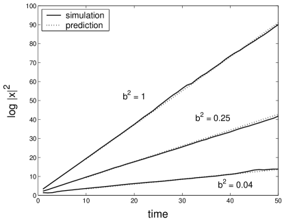
Figure 9: Accuracy of approximation for very ill-conditioned system with large noise

The accuracy of the higher-order approximation method is demonstrated in the simulation of figure 9. In this figure, the second moment of a system with a very poorly-behaved $\mathbf{A}$ (equation 64), subject to normal UH noise with various $b^{2}$, is simulated. The solid lines are the average over 10,000 runs of the simulation, and the dotted lines are the analytical prediction of §5.2.2 for $r=6$. The $\mathbf{A}$ in this system has $v^{2}=170.51$ and so virtually any noise is not treatable using the perturbation approximation. The slopes of the dotted lines are 0.255, 0.833, and 1.794 for $b^{2}=0.04,0.25$, and 1 respectively. Compare to the perturbation approximation which estimates 2.02, 3.85 and 5.24. This system is convergent in mean with $\lambda=0.95$; notice how quickly the moments diverge even for small noise because $v^{2}$ is large.

5.3 Large noise limit

Using the results of the higher order approximation, we can obtain an approximation for the Lyapunov exponent for second moment evolution in the large noise limit.

Note that situations where a small noise has a large effect because the system’s dominant eigenvalue is ill-conditioned (§3) are not treatable using the formalism of this section, for the reasons given below.

5.3.1 Criterion for large noise

A good estimate for the onset of the large noise regime can be obtained by comparing the largest eigenvalue of $\mathbf{A}$ to the average largest eigenvalue of the $\mathbf{B}$.

For independent (UH) noises with variance $b^{2}$ chosen from a normal distribution, the magnitude of the largest eigenvalue of $\mathbf{B}$ is given on average by Geman_largest_eigenvalue

$$\overline{\lambda_{B}}=b\sqrt{n},\;\mbox{ independent noises}$$ (50)

For correlated (T) noises chosen from a normal distribution, the matrix $\mathbf{B}$ is simply a normal random multiple of the matrix $\mathbf{G}$ of all ones. $\mathbf{G}$ has largest eigenvalue $n$ and so the largest eigenvalue of $\mathbf{B}$ is on average

$$\overline{\lambda_{B}}=bn,\;\mbox{ correlated noises}$$ (51)

The large noise case corresponds to $\lambda_{B}\gg\lambda$, that is,

$$n^{k}b^{2}\gg\lambda^{2}$$ (52)

where $k=1$ for independent (UH) noise and $k=2$ for correlated (T) noises.

5.3.2 Lyapunov exponent

To find the Lyapunov exponent for second moment evolution in the large noise limit that $n^{k}b^{2}\gg\lambda^{2}$, we introduce the small parameter

$$\delta=\frac{\lambda^{2}}{n^{k}b^{2}}\ll 1.$$ (53)

We will appeal to the iteration treatment of §5.2.2 which was accurate for any noise. Recall that the Lyapunov exponent is given in this treatment by the log of the largest eigenvalue $\mu_{r}$ of the matrix $M_{r}$ (equation 49), where $r$ is any integer. The approximation is more accurate the larger $r$ is, but as we will see, in the large noise limit there is no need to consider large $r$.

Note that the parameters $\{\alpha_{i}\}$, $f_{u}$, and $f_{v}$ enter into the calculation of $\mu_{r}$ (equation 49). If these parameters are large, they can ruin our expansion since they multiply $\delta$. We therefore assume that they are $O(1)$. Note that this amounts to assuming the system is well-behaved; this is why, as noted above, this expansion is not applicable to ill-conditioned systems.

The characteristic equation for $\mathbf{M}_{r+1}$ can be written

$$0=(\lambda^{2}-\mu)[\mu D_{r}+\alpha_{r}\lambda^{2r}b^{2}f_{u}f_{v}]+\lambda^{2r}b^{2}f_{u}f_{v}$$

where $\mu$ are the eigenvalues and the $D_{r}$ are defined recursively by

$$D_{r+1}=-\mu D_{r}+\alpha_{r}\lambda^{2r}b^{2}f_{u}f_{v}$$

with

$$D_{2}=\det\left(\begin{array}[]{cc}-\mu&f_{v}\alpha_{1}\lambda^{2}/n\\ nf_{u}b^{2}&n^{k}b^{2}-\mu\end{array}\right).$$

Keeping only terms to first order in $\delta$ in the characteristic equation above, we find that the largest eigenvalue $\mu_{r+1}$ is given approximately by

$$\mu_{r+1}^{2}=n^{k}b^{2}\left(\frac{1+\delta+\sqrt{(\delta-1)^{2}+\delta\frac{4\alpha_{1}f_{u}f_{v}}{n}}}{2}\right)$$ (54)

independent of $r$, so that

$$L_{2} \approx \log n^{k}b^{2}+\delta\frac{\alpha_{1}f_{u}f_{v}}{n^{k}}+O(\delta^{2})$$ (55)

$$\approx \log n^{k}b^{2}+\lambda^{2}\frac{\alpha_{1}f_{u}f_{v}}{n^{2k}b^{2}}+O(\lambda^{4}).$$ (56)

Note that the zeroth order term corresponds to that found in the $\mathbf{A}=0$ limit by different means in §2.3.

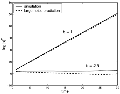
Figure 10: Accuracy (and inaccuracy) of large noise prediction

The range of applicability of the large noise approximation is demonstrated in figure where the second moment is plotted against the prediction of (55). The $\mathbf{A}$ of (63) is used, which has $n=5$ and $\lambda=0.96$. Thus $b=1$ is well within the large noise regime, as shown in the figure. Even $b=0.25$, which is not within the large noise regime, is reasonably well predicted by this approximation.

6 Critical value and stability diagram

As a general rule, large deviations from the average become reasonably likely when the noise is large enough that the second moment diverges. The onset of second moment divergence therefore marks a threshold between two types of behavior and defines a critical value of the size of the noise.

In the case of a homogeneous noise, in which all the noise elements have the same variance $b^{2}$, the critical value can be simply expressed as the value of the variance where the second moment Lyapunov exponent $L_{2}$ equals 1. For a proportional noise, the critical value is the value $q_{c}$ of the constant of proportionality (see table 2) for which $L_{2}=1$. The approaches used in this paper allow for a detailed treatment of the critical value $b_{c}^{2}$ in the case of homogeneous noise, but unfortunately not for proportional or other forms of noise, which is left as a topic for future work. Proportional noise is only discussed in the mean value case where it takes the same form as homogeneous noise.

Throughout this section we will assume that the system is well-behaved, that is, $f_{u}$, $f_{v}$ and the $\{\alpha_{i}\}$ are close to 1. Recall that $f_{u}$ and $f_{v}$ account for the difference between independent and correlated noises, and the $\{\alpha_{i}\}$ measure the accuracy of the approximation (38) for successive powers $\mathbf{A}^{i}$.

6.1 $\lambda^{2}\rightarrow 1$ limit

A limit of particular interest when considering the critical value is $\lambda^{2}\rightarrow 1$, where, as we will see, the critical value drops sharply to 0. Since only small noise is required to cause divergence in this limit, we can apply the first approximation of the iteration treatment, in particular equation 47, to find the critical value

$$(b_{c}^{2})_{\mbox{\footnotesize small noise}}\approx\frac{1}{n^{k}+\frac{f_{u}f_{v}\lambda^{2}}{1-\lambda^{2}}}.$$ (57)

where $k=1$ for independent noises and $k=2$ for correlated noises. The sharp dropoff to 0 of the critical value is evident from this expression and demonstrated in figure 11 below. Note that when $n=1$, in which case $f_{u}=f_{v}=1$ and $\lambda=a$ we retrieve the scalar result $b^{2}_{c}=1-a^{2}$.

Our above expression for $b_{c}^{2}$ should coincide with that implied by the perturbation approximation of §4. Using equation 35 combined with table 3 and definitions (45) and (44) for $f_{u}$ and $f_{v}$, we obtain the perturbation approximation result

$$(b_{c}^{2})_{\mbox{\footnotesize pert}}=\frac{1-\lambda^{2}}{f_{u}f_{v}},$$

which is easily seen to be equivalent to (57) to first order in $(1-\lambda^{2})$.

6.2 $\lambda\longrightarrow 0$ limit

When $\lambda^{2}$ is small and the system well-behaved, the second moment will only diverge if the noise is large. In this case the limit can be obtained from the large noise treatment of §5.3, in particular equation (54) whence we find

$$(b_{c}^{2})_{\mbox{\footnotesize large noise}}\approx\frac{1}{n^{k}+\frac{\alpha_{1}f_{v}f_{u}\lambda^{2}}{1-\lambda^{2}}}.$$ (58)

For well behaved systems with $\alpha_{1}\approx 1$, this expression is almost equivalent to the small noise expression (57)! The scalar result is again retrieved from this expression. We also note that when $\lambda=0$, we obtain the critical value

$$(b_{c}^{2})_{\lambda=0}=1/n^{k},$$

which was obtained in a different way in section 2.3.

6.3 Stability diagram

In the case of a well-behaved system with $\alpha_{1}\approx 1$, the functional form of the critical value is the same for small and large values of $\lambda^{2}$. We thus propose the following expression

$$b_{c}^{2}=\frac{1}{n^{k}+\frac{f_{v}f_{u}\lambda^{2}}{1-\lambda^{2}}}$$ (59)

for the critical value for all ranges of homogeneous noise in well-behaved systems.

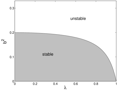
Figure 11: Second moment stability diagram for $n=5$

Using this expression we can make a phase plot for the stability regions of the system, as shown in figure 11 for $n=5$ and independent (UH) noise.

As for proportional noise, we can produce a stability diagram to compare with the homogeneous noise case in the mean value limit. This diagram indicates how large, as a fraction of the size of the unperturbed elements, the noise must be to cause divergence.

Recall that the size of a proportional noise was defined by the factor $q$, the constant of proportionality between the typical noise size and the average element of $\mathbf{A}$ (see table 2). In the mean value approximation, the largest eigenvalue is given approximately by $\lambda\approx an$ and we thus obtain the critical value

$$q_{c}=\frac{n}{\lambda}b_{c}.$$

This relation produces the phase plot of figure 12 for the constant of proportionality $q_{c}$ as a function of $\lambda$.

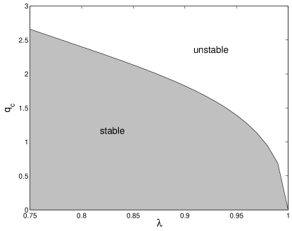
Figure 12: Stability diagram for proportional noise in mean value approximation, $n=5$

6.4 $n$ dependence of critical value

Expression (59) can be used to study the $n$ dependence of the critical value. The $n$ dependence is weak for large $\lambda$, but it is strong when $\lambda$ is small and a large noise is required to cause divergence.

In the limit $\lambda\longrightarrow 1$, where only a small noise is needed to create second moment divergence, it is seen from expression (59) that the $n$ dependence is quite weak. Indeed, the expansion (48) for small noise showed that $n$ dependence enters only in the second order term in this limit. The effects of different forms of noise in this case are quite similar.

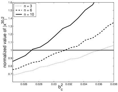
Figure 13: $n$ dependence of critical value

The $n$ dependence of the critical value for small, independent (UH) noises is demonstrated in figure 13. The figure plots the value of the second moment at $t=30$ for systems with various $b$, normalized and averaged over 300,000 runs. Because of the normalization, the initial value (at $t=0$) of the system’s second moment was 1. The critical value $b_{c}^{2}$ is thus indicated for each $n$ by $x$-coordinate for which the plotted curve’s $y$-coordinate begins to exceed 1. Compare the values of $b^{2}_{c}$ given by the simulation to the analytic estimates $b^{2}_{c}=0.0365,0.0326,0.0288$ for $n=3,6,10$, respectively from equation (59). The values of the elements of the $\mathbf{A}$s used in this plot were generated randomly from a normal distribution, and the matrices were normalized to have $\lambda=0.98$.

In the opposite limit of $\lambda\longrightarrow 0$ and large noise, the $n$ dependence is quite strong, as shown in (55). It is in this limit that the difference between independent and correlated noises is quite marked, due to the “destructive interference” phenomenon of independently varying noises discussed previously in §4.4.

6.5 Comparison to convergence bounds

The critical value (59) provides a much more accurate estimate of the “safe” level of noise for which the second moment does not diverge than do the convergence bounds of appendix D. We bring this point up because the traditional mathematical approach to stochastic stability is to use bounds.

These bounds are $b^{2}<\frac{(1-\lambda_{1}^{2})}{n}$ for the second moment (72) and $b^{2}<\frac{(1-\lambda_{1})^{2}}{4n}$ for any moment (71) in the large $n$ limit. For typical well–conditioned systems with $v^{2}$ relatively close to 1 (figure 5, appendix C), it is clear that the critical value is much less restrictive than either of the bounds. That is, the bounds stipulate that we must take a very small noise to guarantee convergence of the second moment; but the critical value indicates that the second moment will converge for a much larger range of noise. When $v^{2}$ is large, $\lambda$ and thus the matrix $\mathbf{A}$ are ill-conditioned and the norm of $\mathbf{A}$ is typically much greater than $\lambda$, so the above bounds are not accurate.

7 Results are generally inapplicable to continuous limit

As a last subject, we discuss the continuous limit of our stochastic system. The results of this paper are not generally applicable in the continuous limit because there is no such thing as small noise, in the sense we have used, in the continuous limit. Of the cases we have considered, the discrete result is only applicable to the continuous limit in the mean value approximation that $\mathbf{A}\approx a\mathbf{G}$.

The reason that the relative size of the noise depends on the time scale is that the correct limit of a white noise process has standard deviation proportional to $\sqrt{dt}$ KloedenPlaten . Thus, the noise necessarily dominates as $dt\rightarrow 0$. To illustrate this point, consider a particle moving in a one dimensional diffusion process

$$dx=((a-1)dt+bdw)x$$

where $dw$ is a Wiener process. When we consider the system’s average motion on a large time scale, the particle generally progresses along the curve $x_{0}e^{(a-1)t}$. However, on very small time scale, the motion is completely erratic because it is dominated by the noise.

For multidimensional systems, the continuous limit of (2) is the stochastic differential equation (in the Ito sense)

$$d\mathbf{x}=[(\mathbf{A}-\mathbf{I})dt+d\mathbf{B}]\mathbf{x}$$ (60)

where $d\mathbf{B}=bd\mathbf{W}$ is a matrix of Wiener processes with mean 0 and standard deviation proportional to $b\sqrt{dt}$, and $\mathbf{I}$ is the identity matrix. Again, in the $dt\rightarrow 0$ limit, the motion is completely dominated by the noise and the vector $\mathbf{x}$ is transformed erratically around in $\mathbf{R}^{n}$. The system can never become aligned with $\mathbf{u}$ because the large noise causes it to couple with the other modes of $\mathbf{A}$. Only when $\lambda_{2}\rightarrow 0$ does the system become aligned with $\mathbf{u}$ and behave similarly to the perturbation approximation, above.

7.1 Correspondence between continuous and discrete results in the mean value approximation

For correspondence between the discrete and continuous cases we consider a system in which $\lambda_{2}=0$: the mean value limit that $\mathbf{A}=a\mathbf{G}$. For this $\mathbf{A}$ and totally correlated noise, an analytic solution to (60) is possible because $\mathbf{A}$ and $d\mathbf{W}=\mathbf{G}dw$ commute Oksendal ; Mao . Here $dw$ is a one-dimensional Wiener process and $\lambda=na$ is the only nonzero eigenvalue of $\mathbf{A}$. The solution to (60) is

$$\mathbf{x}(t)=e^{(\mathbf{A}-\mathbf{I}-b^{2}\mathbf{G}^{2}/2)t+b\mathbf{G}w}\mathbf{x}(0).$$

where $w=\int_{0}^{t}dw$ is normal with variance $t$. From this it is straightforward to calculate that

$$\langle|\mathbf{x}(t)|^{p}\rangle=e^{pt[(na-1)-\frac{n^{2}b^{2}}{2}]}e^{\frac{b^{2}p^{2}n^{2}}{2}t}\left|\frac{1}{n}\mathbf{G}\mathbf{x}(0)\right|^{p}$$

in the asymptotic limit, and the moment Lyapunov exponent is

$$\ell_{p}=-p\delta+p(p-1)\frac{n^{2}b^{2}}{2}$$

where we have taken $\lambda=na=1-\delta$. This can be compared with the discrete result for the mean value limit and totally correlated noise:

$$L_{p}\approx-p\delta+p(p-1)\frac{n^{2}b^{2}}{2}(1-2\delta)+O(\delta^{2})+O(b^{4}),$$

where we have applied $v_{i}=u_{i}=n^{-1/2}$. In the limit of small time step the expressions are equivalent to lowest order. This same analysis can also be performed for a scalar system where there are no other modes to couple to.

7.2 Failure of discrete result in the continuous limit

When there are nonzero modes for $\mathbf{A}$ other that $\lambda$, the discrete result should not, and does not, correspond to the continuous limit. This can be verified by comparison to the result of Arnoldperturbation for small noise moment Lyapunov exponents of arbitrary two-dimensional linear stochastic differential equations. This result, for white noise, is

$$\ell_{p}=-p\delta+p\gamma_{1}\frac{b^{2}}{2}+p^{2}\gamma_{2}\frac{b^{2}}{2}+pO(b^{2})+O(p^{2})$$ (61)

where we take $\lambda=1-\delta$. The $\gamma$ factors depend on the form of noise considered. $\gamma_{2}$ depends only on the dominant eigenmode, while $\gamma_{1}$ depends on both eigenmodes. To proceed we assume UH noise for definiteness, wherein one can show that $\gamma_{2}=v^{2}$. The discrete result (35) for UH noise is

$$L_{p}\approx-p\delta+p(p-1)\frac{v^{2}b^{2}}{2}(1-2\delta)+O(\delta^{2})+O(b^{4}).$$ (62)

Comparing this expression to the continuous version (61), we see that the $1-2\delta$ factor on the noise term accounts for the difference between discrete and continuous evolution, as in §7.1, and that the $p^{2}\gamma_{2}\frac{b^{2}}{2}+pO(b^{2})$ in (61) probably corresponds to the $p(p-1)\frac{v^{2}b^{2}}{2}$ term in (62). Note that the $p(p-1)$ form is present in both continuous scalar and T noise cases and is typical of log-normal distributions.

However, the term in (61) proportional to $\gamma_{1}$ is completely absent in the discrete result; moreover, it depends on $\lambda_{2}$ and its eigenvector which have no effect on the small noise discrete system. This term shows how the solution is coupled to all modes, not just the dominant one, in the continuous limit. In fact, for UH noise, one can show (see (67)) that $\gamma_{1}=1-v^{2}$; in the mean value limit $v^{2}=1$ and the contribution of the second mode is 0.

Appendix A Matrices used to generate figures

All of the unperturbed matrices $\mathbf{A}$ used to generate the figures of this paper were randomly generated. Two particular $\mathbf{A}$s are presented here. The others were generated as described in the text from distributions with low variance, and it would be a waste of space to present them exactly (see discussion in §3.2).

The matrix which was used to generate figure 1 and many others as noted in the text is

$$\footnotesize\mathbf{A}=\left(\begin{array}[]{ccccc}0.1795&0.0861&0.1860&0.0924&0.1661\\ 0.1429&0.1680&0.0517&0.2626&0.3272\\ 0.3558&0.0127&0.2797&0.0221&0.3227\\ 0.2766&0.2654&0.1611&0.0408&0.0745\\ 0.3539&0.3059&0.0596&0.2933&0.3147\\ \end{array}\right).$$ (63)

This matrix has largest eigenvalue $\lambda=0.966$, second largest eigenvalue $|\lambda_{2}|=0.228$, and $v^{2}=1.10$ as computed by Matlab. This matrix is thus quite well-behaved as defined in §3.2.

The matrix with ill-conditioned $\lambda$ used to generate the plot of figure 9 is

$$\footnotesize\mathbf{A}=\left(\begin{array}[]{ccccc}0.5086&0.3496&0.0795&-0.2044&-0.3530\\ -0.6168&0.1553&0.5224&-0.0293&0.0137\\ -0.5526&0.0069&0.0008&-0.3189&0.4345\\ 0.4805&0.8053&-0.5502&0.6173&-0.3041\\ -0.4307&0.8960&0.0255&0.1454&0.6965\\ \end{array}\right)$$ (64)

with largest eigenvalue $\lambda=0.950$, second largest eigenvalue $|\lambda_{2}|=0.888$, and $v^{2}=170.3$ as computed by Matlab.

Appendix B Reduction of nonnegative stability analysis to primitive systems

The reason that $\lambda$ is simple and dominant in all nonnegative systems of interest is that we need only consider systems with primitive $\mathbf{A}$, and primitive matrices have the above property by the Perron-Frobenius theorem. Stability analysis of any nonnegative system whose matrix is not primitive reduces to analysis of primitive subsystems.

More precisely, nonnegative matrices which are not primitive may be either reducible or irreducible imprimitive. Reducible matrices are those which can be written in the form

$$\left(\begin{array}[]{cc}\mathbf{C}&\mathbf{X}\\ \mathbf{0}&\mathbf{D}\end{array}\right),$$ (65)

where $\mathbf{C}$ and $\mathbf{D}$ are square, by renaming the indicesBermanPlemmons . Stability analysis reduces to analysis of the subsystems $\mathbf{C}$ and $\mathbf{D}$, because $\left(\begin{array}[]{cc}\mathbf{C}&\mathbf{X}\\ \mathbf{0}&\mathbf{D}\end{array}\right)^{n}=\left(\begin{array}[]{cc}\mathbf{C}^{n}&\mathbf{Y}\\ \mathbf{0}&\mathbf{D}^{n}\end{array}\right)$. A similar reduction occurs on the subsystems unless they are irreducible. Irreducible imprimitive matrices can be written as

$$\left(\begin{array}[]{ccccc}\mathbf{0}&\mathbf{C}_{12}&\mathbf{0}&\ldots&\mathbf{0}\\ \mathbf{0}&\mathbf{0}&\mathbf{C}_{23}&\ldots&\mathbf{0}\\ \vdots&&\vdots&\ddots&\vdots\\ \mathbf{0}&\mathbf{0}&\mathbf{0}&\ldots&\mathbf{C}_{h-1h}\\ \mathbf{C}_{h1}&\mathbf{0}&\mathbf{0}&\ldots&\mathbf{0}\end{array}\right),$$ (66)

where the 0 blocks along the diagonal are square (second part of Perron Frobenius theorem). The $h$th power of such a matrix is block diagonal and the blocks are primitive BermanPlemmons , so the stability analysis is again reduced.

Physically, primitive matrices have the property that their powers are positive (have no 0 elements). From a physical perspective, primitive systems are thus “fully interacting”. This is in contrast to other nonnegative matrices which have zero blocks when raised to any power.

Appendix C Further discussion of properties of $\mathbf{A}$

There is a correlation between an ill-conditioned $\lambda$ and a small eigenvalue gap. This is so because a matrix with a large $\kappa(\lambda)$ is close to a matrix where $\lambda$ is repeated. In particularGolubbook , there exists a matrix $\mathbf{E}$ such that $\lambda$ is a repeated eigenvalue of $\mathbf{A}+\mathbf{E}$ and

$$|\mathbf{E}|\leq\frac{|\mathbf{A}|}{\sqrt{(\kappa(\lambda))^{2}-1}}.$$

However, $\kappa(\lambda)$ may be small even if the gap is small. The relation between $\kappa(\lambda)$ and the eigenvalue gap is shown in figure 5, above.

There is also a correlation between normality of $\mathbf{A}$ and a small $\kappa(\lambda)$. When $\mathbf{A}$ is normal, that is, $\mathbf{A}\mathbf{A}^{T}=\mathbf{A}^{T}\mathbf{A}$, all of its eigenvectors are orthogonal and all the eigenvalues are perfectly conditioned. However, $\kappa(\lambda)$ may be small in matrices which are far from normal. The relation between $\kappa(\lambda)$ and the normality of $\mathbf{A}$ is shown in figure 14.

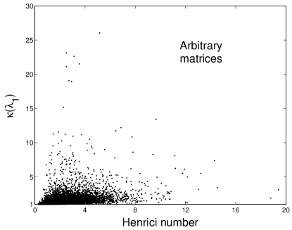
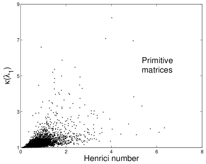
Figure 14: Scatter plots of $|\mathbf{v}|$ versus the Henrici number $|\mathbf{A}\mathbf{A}^{T}-\mathbf{A}^{T}\mathbf{A}|$, a measure of non-normality, for 10,000 randomly generated $5\times 5$ matrices normalized so that $\lambda=1$. At left the elements were chosen from a normal distribution and only plotted if $\lambda$ was real. At right, the matrices are nonnegative primitive; a random number of elements were 0, and the nonzero elements were chosen from a uniform distribution.

Another way to characterize $\kappa$ is the relation

$$v^{2}=1-\sum_{i\neq 1}(\mathbf{u}\cdot\mathbf{e}^{R}_{i})(\mathbf{v}\cdot\mathbf{e}^{L}_{i})$$ (67)

where $\mathbf{e}^{R}_{i}$ is the $i$th column of $\mathbf{P}$ (the right eigenvector corresponding to $\lambda_{i}$) and $\mathbf{e}^{L}_{i}$ is the $i$th row of $\mathbf{P}^{-1}$ (the left eigenvector corresponding to $\lambda_{i}$) This relation is established by noting that $\sum_{ij}\mathbf{e}^{R}_{i}\mathbf{e}^{R}_{j}\mathbf{e}^{L}_{i}\mathbf{e}^{L}_{j}=1$. It shows how $v^{2}$ is related to the angles between the eigenvectors. In particular, we see that for a normal matrix where the eigenvectors are orthogonal, $v^{2}=1$; but in general, the angular distribution of the eigenvalues is complicated.

Finally, there is a correlation between $|\lambda_{2}|\rightarrow 0$ and the variance $\sigma_{A}^{2}$ of the elements of $\mathbf{A}$. Bounds for the second largest eigenvalue can be found in the case of row (or column) stochastic matrices, for exampleBermanPlemmons : $|\lambda_{2}|\leq\min\big{(}1-\sum_{i}\min_{j}A_{ij},\sum_{i}\max_{j}A_{ij}-1\big{)}$. This shows that, at least for stochastic matrices, a small variance $\sigma_{A}^{2}$ corresponds to a large eigenvalue gap. This is shown to be true for all matrices in figure 15. Of course, the converse is not true; matrices with large $\sigma_{A}^{2}$ can also have a large eigenvalue gap, as also is shown in figure 15.

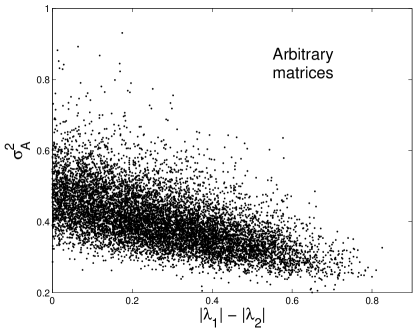
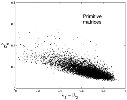
Figure 15: Scatter plots of eigenvalue gap $\lambda-|\lambda_{2}|$ versus standard deviation of the $\mathbf{A}_{ij}$ for 10,000 randomly generated $5\times 5$ matrices, normalized so that $\lambda=1$. At left the elements were chosen from a normal distribution and only plotted if $\lambda$ is real. At right, the matrices are nonnegative primitive; a random number of elements were 0, and the nonzero elements were chosen from a uniform distribution.

Appendix D Bounds on convergence of $\langle|\mathbf{x}|^{2}\rangle$

In this section we apply the matrix 2-norm to determine two different bounds on the variance of the noise which, if satisfied, ensure the convergence of $\langle|\mathbf{x}|^{2}\rangle$. These conditions are sufficient but by no means necessary. The second moment will of course never converge if the system does not converge in mean. We therefore take $\lambda<1$ in this section.

The norm of a matrix is any function satisfying the regular properties of a vector norm and additionally the inequality $|\mathbf{A}\mathbf{B}|\leq|\mathbf{A}||\mathbf{B}|$. The matrix 2-norm corresponding to the usual Euclidean vector norm is

$$|\mathbf{A}|_{2}=(\rho(\mathbf{A}\mathbf{A}^{*}))^{1/2}.$$ (68)

where $\rho$ is the spectral radius. Note that for any norm, $|A|\geq|\mathbf{x}\mathbf{A}|/|\mathbf{x}|=|\lambda|$ for any eigenvalue $\lambda$, so that in particular,

$$\lambda\leq|\mathbf{A}|.$$ (69)

For ill-conditioned matrices, which includes those with ill-conditioned $\lambda$, $|\mathbf{A}|$ is typically much larger than $\lambda$ Golubbook .

D.1 Bound on convergence of any moment

We have $|\mathbf{x}^{t+1}|^{p}\leq{|\mathbf{A}+\mathbf{B}^{t}|}^{p}|\mathbf{x}^{t}|^{p}$, so that

$$\langle|\mathbf{x}^{t}|^{p}\rangle\leq\left[\prod_{\tau=1}^{t-1}\langle|\mathbf{A}+\mathbf{B}^{\tau}|\rangle^{p}\right]|\mathbf{x}^{0}|^{p}$$

where the expected value goes inside the product because the noise is white noise. $\langle|\mathbf{x}|^{p}\rangle$ will thus converge for any $p$ provided that $\langle|\mathbf{A}+\mathbf{B}|\rangle<1$ (we neglect the time superscript because the noise is stationary), or more usefully

$$\langle|\mathbf{B}|\rangle<1-|\mathbf{A}|.$$ (70)

using $|\mathbf{A}+\mathbf{B}|\leq|\mathbf{A}|+|\mathbf{B}|$. Since convergence of every moment is a much stronger condition than convergence of just the second moment, this bound is typically poor when applied to the second moment.

We may estimate a lower limit for this bound for well-conditioned systems in the large $n$ limit when the noise is UH (uncorrelated $B_{ij}$ all with the same variance $b^{2}$). We do so by using $|\mathbf{A}|>\lambda$ (equation 69) and a result of Geman that $\liminf|\mathbf{B}|\geq 2b\sqrt{n}$ almost surely in the large $n$ limit, provided that the elements of $\mathbf{B}$ are mean 0 i.i.d. and their moments do not grow too fast (which is satisfied for any reasonable noise). Thus

$$\lambda_{1}+2b\sqrt{n}\leq|\mathbf{A}|+\langle|\mathbf{B}|\rangle$$

and the condition (70) on $b$ for convergence at least weaker than

$$b^{2}<\frac{(1-\lambda_{1})^{2}}{4n}$$ (71)

in the large $n$ limit. That is to say, (70) is more restrictive on $b$ than (71). For ill-conditioned systems, (71) may not be accurate because $|\mathbf{A}|$ may be much larger than $\lambda$.

D.2 Second moment bound

A different bound on the convergence of the second moment in the case of UH noise can be found by applying the expected value before taking norms. We have

$$\langle|\mathbf{x}^{t}|^{2}\rangle = \langle|(\mathbf{A}+\mathbf{B}^{t})\mathbf{x}^{t-1}|^{2}\rangle$$

$$\leq (|\mathbf{A}|^{2}+nb^{2})\langle|\mathbf{x}^{t-1}|^{2}\rangle$$

where we have used the properties of the norm and the fact that the noise is UH, white and has mean 0. We thus have the convergence condition $|\mathbf{A}|^{2}+nb^{2}<1$, or

$$b^{2}<\frac{(1-|\mathbf{A}|^{2})}{n}$$

for the convergence of $\langle|x|^{2}\rangle$. Note that this condition is at least weaker than the condition

$$b^{2}<\frac{(1-\lambda_{1}^{2})}{n}$$ (72)

because of (69). Again, (72) may not be accurate for ill-conditioned $\mathbf{A}$ because $|\mathbf{A}|$ may be much larger than $\lambda$.

References

- (1) J. Guckenheimer, Lectures in Applied Math 17, 187 (1979).
- (2) C. W. Gardiner, Handbook of Stochastic Methods for Physics, Chemistry and the Natural Sciences, 2nd ed. (Springer-Verlag, Berlin, 1985).
- (3) J. A. Rice, Mathematical Statistics and Data Analysis, 2nd ed. (Duxbury Press, Belmont, California, 1995).
- (4) S. Redner, American Journal of Physics 53, 267 (1990).
- (5) R. C. Lewontin and D. Cohen, Proceedings of the National Academy of Sciences 62, 1056 (1969).
- (6) L. Arnold and V. Wihstutz, editors, Lyapunov Exponents, Lecture Notes in Mathematics Vol. 1186 (Springer, New York, 1986).
- (7) J. N. Tsitsiklis and V. D. Blondel, Mathematics of Control, Signals, and Systems 10, 31 (1997).
- (8) P. Bougerol and J. Lacroix, Products of Random Matrices with Applications to Schrödinger Operators (Birkhäuser, Boston, 1985).
- (9) G. W. Stewart, University of Maryland Institute for Advanced Computer Studies Report No. 91, 2001 (unpublished), To appear in Numerische Mathematik.
- (10) J. E. Cohen and C. M. Newman, The Annals of Probability 12, 283 (1984).
- (11) L. Gurvits, Linear Algebra and its Applications 231, 47 (1995).
- (12) N. E. Barabanov, Automation and Remote Control 49, 152 (1988).
- (13) D. Hinrichsen and N. K. Son, International Journal of Robust and Nonlinear Control 1, 79 (1991).
- (14) D. Hinrichsen and N. K. Son, Stability radii of positive discrete-time systems, in Proceedings of the Third International Conference on Approximation and Optimization, edited by B. Bank et al., All ACM Conferences, The Electronic Library of Mathematics (1997), 1995.
- (15) P. R. Kumar and P. Varaiya, Stochastic Systems: Estimation, Identification and Adaptive Control (Prentice-Hall, Englewood Cliffs, New Jersey, 1986).
- (16) C. Xiao, D. J. Hill, and P. Agathoklis, IEEE Transactions on Circuits and Systems 44, 614 (1997).
- (17) G. V. Moustakidis, International Journal of Adaptive Control and Signal Processing 12, 579 (1998).
- (18) M. Milisavljević and E. I. Verriest, Stability and stabilization of discrete systems with multiplicative noise, in Proceedings of the European Control Conference, 1997.
- (19) A. Crisanti, G. Paladin, and A. Vulpiani, Products of Random Matrices in Statistical Physics (Springer-Verlag, Berlin, 1993).
- (20) N. G. van Kampen, Stochastic Processes in Physics and Chemistry (North-Holland, Amsterdam, 1992).
- (21) F. Ma and T. K. Caughey, International Journal of Nonlinear Mechanics 16, 139 (1981).
- (22) F. Kozin, Automatica 5, 95 (1969).
- (23) W. M. Haddad, V. Chellaboina, and S. G. Nersesov, Mathematical Problems in Engineering 8, 493 (2002).
- (24) T. Hogg, B. A. Huberman, and J. M. McGlade, Proceedings of the Royal Society of London B237, 43 (1989).
- (25) R. Z. Khas’minskii, Prikladnaya matematika i mekhanika (Journal of applied mathematics and mechanics) 31, 1021 (1967).
- (26) X. Mao, Stochastic Differential Equations and Applications (Horwood, Chichester, 1997).
- (27) L. Arnold, M. M. Doyle, and N. S. Namachchivaya, Dynamics and Stability of Systems 12, 187 (1997).
- (28) G. Strang, Linear Algebra and Its Applications (Academic Press, New York, 1976).
- (29) A. Berman, M. Neumann, and R. J. Stern, Nonnegative Matrices in Dynamic Systems (John Wiley and Sons, New York, 1989).
- (30) L. Farina and S. Rinaldi, Positive Linear Systems: Theory and Applications (John Wiley and Sons, New York, 2000).
- (31) L. Benvenuti, A. de Santis, and L. Farina, editors, Positive Systems, , Lecture Notes in Control and Information Sciences Vol. 294, Berlin, 2003, Springer.
- (32) L. N. Trefethen, A. E. Trefethen, S. C. Reddy, and T. A. Driscoll, Science 261, 578 (1993).
- (33) R. Bellman, Duke Mathematical Journal 21, 491 (1954).
- (34) H. Furstenberg and H. Kesten, Annals of Mathematical Statistics 31, 457 (1960).
- (35) G. H. Golub and C. F. van Loan, Matrix Computations, 2nd ed. (The Johns Hopkins University Press, Baltimore, 1989).
- (36) A. Edelman, Eigenvalues and Condition Numbers of Random Matrices, PhD dissertation, MIT, 1989.
- (37) H. Minc, Nonnegative Matrices (John Wiley and Sons, New York, 1988).
- (38) F. Juhasz, Discrete Mathematics 41, 161 (1982).
- (39) Y. B. Zel’dovich, S. A. Molchanov, A. A. Ruzmaikin, and D. D. Sokolov, Uspekhi Fizicheskikh Nauk 152, 3 (1987).
- (40) Z. Füredi and J. Komlós, Combinatorica 1, 233 (1981).
- (41) S. Roy, Moment-Linear Stochastic Systems and Their Applications, PhD dissertation, MIT, 2003.
- (42) S. Geman, Ann. Probab. 14, 1318 (1986).
- (43) P. E. Kloeden and E. Platen, Numerical Solution of Stochastic Differential Equations (Springer-Verlag, Berlin, 1992).
- (44) B. K. Øksendal, Stochastic Differential Equations: an Introduction with Applications, 6th ed. (Springer, Berlin, 2003).
- (45) A. Berman and R. J. Plemmons, Nonnegative Matrices in the Mathematical Sciences (Academic Press, New York, 1979).
- (46) S. Geman, The Annals of Probability 8, 252 (1980).