On the resolvent and spectral functions of a second order differential operator with a regular singularity

Abstract.

We consider the resolvent of a second order differential operator with a regular singularity, admitting a family of self-adjoint extensions. We find that the asymptotic expansion for the resolvent in the general case presents unusual powers of $\lambda$ which depend on the singularity. The consequences for the pole structure of the $\zeta$-function, and for the small-$t$ asymptotic expansion of the heat-kernel, are also discussed.

1. Introduction

It is well known that in Quantum Field Theory under external conditions, quantities like vacuum energies and effective actions, which describe the influence of boundaries or external fields on the physical system, are generically divergent and require a renormalization to get a physical meaning.

In this context, a powerful and elegant regularization scheme to deal with these problems is based on the use of the $\zeta$-function [1, 2] or the heat-kernel (for recent reviews see, for example, [3, 4, 5, 6, 7]) associated to the relevant differential operators appearing in the quadratic part of the actions. In this way, ground state energies, heat-kernel coefficients, functional determinants and partition functions for quantum fields can be given in terms of the corresponding $\zeta$-function, where the ultraviolet divergent pieces of the one-loop contributions are encoded as poles of its holomorphic extension.

Thus, it is of major interest in Physics to determine the singularity structure of $\zeta$-functions associated with these physical models.

In particular [8], for an elliptic boundary value problem in a $\nu$-dimensional compact manifold with boundary, described by a differential operator $A$ of order $\omega$, with smooth coefficients and a ray of minimal growth, defined on a domain of functions subject to local boundary conditions, the $\zeta$-function

(1.1) $$\zeta_{A}(s):=Tr\{A^{-s}\}$$

has a meromorphic extension to the complex $s$-plane whose singularities are isolated simple poles at $s=(\nu-j)/\omega$, with $j=0,1,2,\dots$

In the case of positive definite operators, the $\zeta$-function is related, via Mellin transform, to the trace of the heat-kernel of the problem, and the pole structure of $\zeta_{A}(s)$ determines the small-$t$ asymptotic expansion of this trace [8, 9]:

(1.2) $$Tr\{e^{-tA}\}\sim\sum_{j=0}^{\infty}a_{j}(A)\,t^{(j-\nu)/\omega},$$

where the coefficients are related to the residues by

(1.3) $$a_{j}(A)=\left.{\rm Res}\right|_{s=(\nu-j)/\omega}\Gamma(s)\,\zeta_{A}(s).$$

For operators of the form $-\partial_{x}^{2}+V(x)$ with a singular potential $V(x)$ asymptotic to $\kappa/x^{2}$ as $x\rightarrow 0$, this expansion is substantially different. If $\kappa\geq 3/4$, the operator is essentially self-adjoint. This case has been treated in [10, 11, 12], where log terms are found, as well as terms with coefficients which are distributions concentrated at the singular point $x=0$. For the case $\kappa>-1/4$, the Friedrichs extension has been treated in [13] for operators in $\mathbf{L_{2}}(0,1)$, and in [14] for operators in $\mathbf{L_{2}}(\mathbf{R^{+}})$, making use of the scale invariance of the operator domain and explicit representations of the resolvent. Moreover, as a particular case of a manifold with an isolated conic singularity, reference [15] gave a description of the boundary behavior of the Friedrichs heat-kernel which does not make use of the resolvent, and showed vía boundary maps how it can be used to construct the heat-kernel for other self-adjoint extensions of these operators, showing explicitly the first two terms in the asymptotic expansion of the trace of their difference.

On the other hand, reference [16] gave the pole structure of the $\zeta$-function of a second order differential operator defined on the (non compact) half-line $\mathbf{R}^{+}$, having a singular zero-th order term $V(x)=\kappa\,x^{-2}+x^{2}$. It showed that, for a certain range of real values of $\kappa$, this operator admits nontrivial self-adjoint extensions in $\mathbf{L_{2}}(\mathbf{R^{+}})$, for which the associated $\zeta$-function (given by an integral representation) presents isolated simple poles which (in general) do not lie at $s=(1-j)/2$ for $j=0,1,\dots$ (as would be the case for a regular $V(x)$), and can even take irrational values.

A similar structure has been noticed in [17] for the singularities of the $\zeta$ and $\eta$-functions of a system of first order differential operators with a singular zero-th order term $\sim g\,x^{-1}$, which also admits a family of self-adjoint extensions for real $g$ taking values in certain range. It has been shown that, in the general case, the asymptotic expansion of the resolvent contains $g-$dependent powers of $\lambda$ which make the $\zeta$ and $\eta$-functions to present poles lying at points which depend on the singularity, with residues depending on the self-adjoint extension.

Let us mention that singular potentials $\sim 1/x^{2}$ have been considered in the description of several physical systems, like the Calogero Model [18, 19, 16, 20], conformal invariant quantum mechanical models [21, 22, 23] and, more recently, the dynamics of quantum particles in the asymptotic near-horizon region of black-holes [24, 25, 26, 27, 28]. The self-adjoint extensions of these operators have also been considered in [29]. Moreover, singular superpotentials has been considered as possible agents of supersymmetry breaking in models of Supersymmetric Quantum Mechanics [30, 31, 32].

It is the aim of the present article to analyze the behavior of the resolvent, the $\zeta$-function and the trace of the heat-kernel of a second order differential operator with a regular singularity in a compact segment, $D_{x}=-\partial_{x}^{2}+{g(g-1)}\,{x^{-2}}$, for those values of $g$ for which it admits a family of self-adjoint extensions.

Following the scheme developed in [17], we will show that the asymptotic expansion for the resolvent in the general case presents powers of $\lambda$ which depend on the singularity, and can even take irrational values. The consequence of this behavior on the corresponding $\zeta$-function is the presence of simple poles lying at points which also depend on the singularity, with residues depending on the self-adjoint extension considered.

We first construct the resolvents for two particular extensions, for which the boundary condition at the singular point $x=0$ is invariant under the scaling $x\rightarrow c\,x$. The resolvent expansion for these special extensions displays the usual powers, leading to the usual poles for the $\zeta$-function (and the usual structure for the asymptotic expansion of the heat-kernel trace).

The resolvents of the remaining extensions are convex linear combinations of these special extensions, but the coefficients in the convex combination depend on the eigenvalue parameter $\lambda$. This dependence leads to unusual powers in the resolvent expansion, and hence to unusual poles for the zeta-function (and unusual powers in the asymptotic expansion of the heat-kernel trace).

These self-adjoint extensions are not invariant under the scaling $x\rightarrow c\,x$. As $c\rightarrow 0$ they tend (at least formally) to one of the invariant extensions, and as $c\rightarrow\infty$ they tend to the other. As $c\rightarrow 0$ the residues at the anomalous poles tend to zero, whereas as $c\rightarrow\infty$ these residues become infinite. The way these residues depend on the boundary condition is explained by a scaling argument in Section 7.

The structure of the article is as follows: In Section 2 we define the operator and determine its self-adjoint extensions for $\frac{1}{2}<g<\frac{3}{2}$, and in Section 3 we study their spectra. In Section 4 we construct the resolvent for a general extension as a linear combination of the resolvent of two limiting cases, and in Section 5 we consider the traces of these operators. The asymptotic expansions of these traces, evaluated in Section 6, are used in Section 7 to construct the associated $\zeta$-function and study its singularities, as well as the small-t asymptotic expansion of the heat-kernel trace. The special case $g=\frac{1}{2}$ is considered in Appendix A.

2. The operator and its self-adjoint extensions

Let us consider the differential operator

(2.1) $$D_{x}=-\frac{d^{2}}{dx^{2}}+\frac{g(g-1)}{x^{2}}\,,$$

with $g\in\mathbb{R}$, defined on a domain of smooth functions with compact support in a segment, $\mathcal{D}(D)=\mathcal{C}_{0}^{\infty}(0,1)$. It can be easily seen that $D_{x}$ so defined is symmetric.

The adjoint operator $D_{x}^{*}$, which is the maximal extension of $D_{x}$, is defined on the domain $\mathcal{D}(D_{x}^{*})$ of functions $\phi(x)\in\mathbf{L_{2}}(0,1)$, having a locally sumable second derivative and such that

(2.2) $$D_{x}\phi(x)=-\phi^{\prime\prime}(x)+\frac{g(g-1)}{x^{2}}\,\phi(x)=f(x)\in\mathbf{L_{2}}(0,1)\,.$$

Lemma 2.1.

If $\phi(x)\in\mathcal{D}(D_{x}^{*})$ and $\frac{1}{2}<g<\frac{3}{2}$, then

(2.3) $${\left|\,\phi(x)-\left(\frac{C_{1}[\phi]\,x^{g}+C_{2}[\phi]\,x^{1-g}}{\sqrt{2g-1}}\right)\right|\leq\frac{\|D_{x}\phi(x)\|}{(3/2-g)\sqrt{2g+1}}\ x^{3/2}}$$

and

(2.4) $${\left|\,\phi^{\prime}(x)-\left(\frac{g\,C_{1}[\phi]\,x^{g-1}+(1-g)\,C_{2}[\phi]\,x^{-g}}{\sqrt{2g-1}}\right)\right|\leq\frac{3/2\,\|D_{x}\phi(x)\|}{(3/2-g)\sqrt{2g+1}}\ x^{1/2}}$$

for some constants $C_{1}[\phi]$ and $C_{2}[\phi]$, where $\|\cdot\|$ is the $\mathbf{L_{2}}$-norm.

Proof: Let us write $\phi(x)=x^{g}u(x)$. Then, Eq. (2.2) implies

(2.5) $$\begin{array}[]{c}\displaystyle{u^{\prime}(x)=K_{2}\,x^{-2g}-x^{-2g}\,\int_{0}^{x}y^{g}\,f(y)\,dy\,,}\\ \\ \displaystyle{u(x)=K_{1}+\frac{K_{2}}{1-2g}\,x^{1-2g}-\int_{0}^{x}y^{-2g}\,\int_{0}^{y}z^{g}\,f(z)\,dz\ dy\,,}\end{array}$$

for some constants $K_{1}$ and $K_{2}$. Now, taking into account that

(2.6) $$\begin{array}[]{c}\displaystyle{\left|\int_{0}^{x}y^{g}\,f(y)\,dy\right|\leq\frac{x^{g+1/2}}{\sqrt{2g+1}}\,\|f\|}\,,\\ \\ \displaystyle{\left|\int_{0}^{x}y^{-2g}\int_{0}^{y}z^{g}\,f(z)\,dz\,dy\right|\leq\frac{x^{3/2-g}}{(3/2-g)\sqrt{2g+1}}\,\|f\|}\,,\end{array}$$

we immediately get Eqs. (2.3) and (2.4).

Lemma 2.2.

Let $\phi(x),\psi(x)\in\mathcal{D}(D^{*})$ and $\frac{1}{2}<g<\frac{3}{2}$. Then

(2.7) $$\begin{array}[]{c}\left(D_{x}\psi,\phi\right)-\left(\psi,D_{x}\phi\right)=\\ \\ =\Big{\{}C_{1}[\psi]^{*}C_{2}[\phi]-C_{2}[\psi]^{*}C_{1}[\phi]\Big{\}}+\Big{\{}\psi(1)^{*}\,\phi^{\prime}(1)-\psi^{\prime}(1)^{*}\,\phi(1)\Big{\}}\,.\end{array}$$

Proof: From Eq. (2.2) one easily obtains

(2.8) $$\begin{array}[]{c}\left(D_{x}\psi,\phi\right)-\left(\psi,D_{x}\phi\right)=\\ \\ =\displaystyle{\lim_{\varepsilon\rightarrow 0^{+}}\int_{\varepsilon}^{1}\partial_{x}\Big{\{}\psi(x)^{*}\,\phi^{\prime}(x)-\psi^{\prime}(x)^{*}\,\phi(x)\Big{\}}\,dx}\,,\end{array}$$

from which, taking into account the results in Lemma 2.1, Eq. (2.7) follows directly.

Now, if $\psi(x)$ in Eq. (2.7) belongs to the domain of the closure of $D_{x}$, $\overline{D}_{x}=(D_{x}^{*})^{*}$,

(2.9) $$\psi(x)\in\mathcal{D}(\overline{D}_{x})\subset\mathcal{D}(D_{x}^{*})\,,$$

then the right hand side of Eq. (2.7) must vanish for any $\phi(x)\in\mathcal{D}(D_{x}^{*})$. Therefore

(2.10) $$C_{1}[\psi]=C_{2}[\psi]=\psi(1)=\psi^{\prime}(1)=0\,.$$

On the other hand, if $\psi(x),\phi(x)$ belong to the domain of a symmetric extension of $D_{x}$ (contained in $\mathcal{D}(D_{x}^{*})$), the right hand side of Eq. (2.7) must also vanish.

Thus, the closed extensions of $D_{x}$ correspond to the subspaces of $\mathbb{C}^{4}$ under the map $\Phi\rightarrow\left(C_{1}[\Phi],C_{2}[\Phi],\phi(1),\phi^{\prime}(1)\right)$, and the self-adjoint extensions correspond to those subspaces $S\subset\mathbb{C}^{4}$ such that $S=S^{\perp}$, with the orthogonal complement taken in the sense of the symplectic form on the right hand side of Eq. (2.7).

For definiteness, in the following we will consider self-adjoint extensions satisfying the local boundary condition

(2.11) $$\phi(1)=0\,.$$

Each such extension is determined by a condition of the form

(2.12) $$\alpha\,C_{1}[\Phi]+\beta\,C_{2}[\Phi]=0\,,$$

with $\alpha,\beta\in\mathbb{R}$, and $\alpha^{2}+\beta^{2}=1$. We denote this extension by $D_{x}^{(\alpha,\beta)}$.

3. The spectrum

In order to determine the spectrum of the self-adjoint extensions of $D_{x}$ for $\frac{1}{2}<g<\frac{3}{2}$, we need the solutions of

(3.1) $$(D_{x}-\lambda)\phi_{\lambda}(x)=0\,,$$

satisfying the boundary conditions in Eqs. (2.11) and (2.12).

The general solution of the homogeneous equation for $\lambda=0$ is

(3.2) $$\phi_{0}(x)=\frac{1}{\sqrt{2g-1}}\left(C_{1}\,x^{g}+C_{2}\,x^{1-g}\right)\,,$$

and the boundary conditions in Eqs. (2.11) and (2.12) imply that

(3.3) $$C_{1}+C_{2}=0\,,\quad\alpha\,C_{1}+\beta\,C_{2}=0\,.$$

Consequently, there are no zero modes except for the self-adjoint extension characterized by $\alpha=\beta=1/\sqrt{2}$.

For $\lambda\neq 0$, the solutions of Eq. (3.1) are of the form

(3.4) $$\begin{array}[]{c}\displaystyle{\phi(x)=\frac{{C}_{1}}{{\sqrt{2\,g-1}}}\,\frac{\Gamma(\frac{1}{2}+g)}{2^{\frac{1}{2}-g}\,{\mu}^{g-\frac{1}{2}}}\,{\sqrt{x}}\,J_{g-\frac{1}{2}}(\mu\,x)+}\\ \\ \displaystyle{+\frac{{C}_{2}}{{\sqrt{2\,g-1}}}\,\frac{\Gamma(\frac{3}{2}-g)}{2^{g-\frac{1}{2}}\,{\mu}^{\frac{1}{2}-{g}}}\,{\sqrt{x}}\,J_{\frac{1}{2}-g}(\mu\,x)\,,}\end{array}$$

where $\mu=+\sqrt{\lambda}$, and the $\mu$-dependent coefficients have been introduced for later convenience.

Taking into account that

(3.5) $$J_{\nu}(z)=z^{\nu}\,\left\{\frac{1}{2^{\nu}\,\Gamma(1+\nu)}+O(z^{2})\right\}\,,$$

we get from Eqs. (2.3) and (2.12)

(3.6) $$\alpha\,C_{1}+\beta\,C_{2}=0\,.$$

On the other hand, the condition in Eq. (2.11) implies

(3.7) $$\begin{array}[]{c}\displaystyle{\phi(1)=\frac{{C}_{1}}{{\sqrt{2\,g-1}}}\,\frac{\Gamma(\frac{1}{2}+g)}{2^{\frac{1}{2}-g}\,{\mu}^{g-\frac{1}{2}}}\,J_{g-\frac{1}{2}}(\mu)+}\\ \\ \displaystyle{+\frac{{C}_{2}}{{\sqrt{2\,g-1}}}\,\frac{\Gamma(\frac{3}{2}-g)}{2^{g-\frac{1}{2}}\,{\mu}^{\frac{1}{2}-{g}}}\,J_{\frac{1}{2}-g}(\mu)=0\,.}\end{array}$$

For $\alpha=0$, Eq. (3.6) implies $C_{2}=0$ (Dirichlet boundary conditions at the origin). Therefore, $\phi(1)=0\Rightarrow J_{g-\frac{1}{2}}(\mu)=0$. Thus, the spectrum of this self-adjoint extension is positive and non-degenerate, with the eigenvalues of $D_{x}^{D}:=D_{x}^{(0,1)}$ given by

(3.8) $$\lambda_{n}=j_{g-\frac{1}{2},n}^{2}\,,\quad n=1,2,\dots\,,$$

where $j_{\nu,n}$ is the $n$-th positive zero of the Bessel function $J_{\nu}(z)$.

For $\alpha\neq 0$, from Eqs. (3.6) and (3.7) we easily get the following transcendental equation for the eigenvalues of $D_{x}^{(\alpha,\beta)}$:

(3.10) $$F(\mu):={\mu}^{2\,g-1}\,\frac{J_{\frac{1}{2}-g}(\mu)}{J_{g-\frac{1}{2}}(\mu)}=\rho(\alpha,\beta)\,,$$

where we have defined

(3.11) $$\rho(\alpha,\beta):=\frac{\beta}{\alpha}\ \frac{2^{2\,g-1}\,\Gamma(\frac{1}{2}+g)}{\Gamma(\frac{3}{2}-g)}\,.$$

For the positive eigenvalues ${\lambda}=\mu^{2}$, both sides in Eq. (3.10) have been plotted in Figure 1, for particular values of $\rho(\alpha,\beta)$ and $g$.

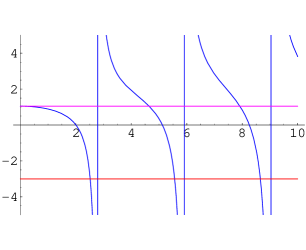
Figure 1. Plot for $F(\mu)$, $\rho(\alpha,\beta)=-3$ and $\displaystyle{\rho(\alpha,\alpha)}$, with $g=3/4$.

Moreover, if $\beta/\alpha>1\Rightarrow\rho(\alpha,\beta)>\rho(\alpha,\alpha)$, and the extension $D_{x}^{(\alpha,\beta)}$ has a negative eigenvalue. Indeed, if $\lambda_{-}=(i\mu)^{2}<0$, then

(3.12) $$\begin{array}[]{c}\displaystyle{F(i\,\mu)={\mu}^{2\,g-1}\,\frac{I_{\frac{1}{2}-g}(\mu)}{I_{g-\frac{1}{2}}(\mu)}=}\\ \\ \displaystyle{=2^{2\,g-1}\,\frac{\Gamma(\frac{1}{2}+g)}{\Gamma(\frac{3}{2}-g)}\left\{1+\frac{\left(2\,g-1\right)\,{\mu}^{2}}{\left(3-2\,g\right)\,\left(1+2\,g\right)}+{O}(\mu^{4})\right\}}\,,\end{array}$$

where $I_{\nu}(\mu)$ is the modified Bessel function. For a plot, see Figure 2.

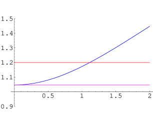
Figure 2. Plot for $F(i\,\mu)$, $\rho(\alpha,\beta)=1.2$ and $\displaystyle{\rho(\alpha,\alpha)}$, with $g=3/4$.

Notice that the spectrum is always non-degenerate, and there is a positive eigenvalue between each pair of consecutive squared zeroes of $J_{g-\frac{1}{2}}(\lambda)$. Therefore, from Eq. (3.9) we get $\lambda_{n}=\pi^{2}\,n^{2}+O(n)$.

In particular, for the $\beta=0$ extension (which we call the “N-extension”), $D_{x}^{N}:=D_{x}^{(1,0)}$, it can be seen fron Eq. (3.10) that the eigenvalues are given by

(3.13) $$\lambda_{n}=j_{\frac{1}{2}-g,n}^{2}\,,\ n=1,2,\dots\,,$$

where $j_{\frac{1}{2}-g,n}^{2}$ are the positive zeroes of $J_{\frac{1}{2}-g}(\mu)$.

4. The resolvent

In this Section we will construct the resolvent of $D_{x}$,

(4.1) $$G(\lambda)=(D_{x}-\lambda)^{-1}\,,$$

for its different self-adjoint extensions when $\frac{1}{2}<g<\frac{3}{2}$.

We will first consider the two limiting cases in Eq. (2.12), namely the “$D$-extension”, for which $\alpha=0\Rightarrow C_{2}[\phi]=0$, and the “$N$-extension”, with $\beta=0\Rightarrow C_{1}[\phi]=0$. The resolvent for a general self-adjoint extension will be later evaluated as a linear combination of those obtained for these two limiting cases.

For the kernel of the resolvent we have

(4.2) $$(D_{x}-\mu^{2})\,G(x,y;\mu^{2})=\delta(x-y)\,,$$

where $\mu^{2}=\lambda$, with $-\pi/2<{\rm arg}(\mu)\leq\pi/2$.

To proceed, we need some particular solutions of the homogeneous equation (3.1). Then, let us define

(4.3) $$\left\{\begin{array}[]{l}\displaystyle{L^{D}(x,\mu)={\sqrt{x}}\,J_{g-\frac{1}{2}}(\mu\,x)\,,}\\ \\ \displaystyle{L^{N}(x,\mu)={\sqrt{x}}\,J_{\frac{1}{2}-g}(\mu\,x)\,,}\\ \\ \displaystyle{R(x,\mu)={\sqrt{x}}\,\left(J_{\frac{1}{2}-g}(\mu)\,J_{g-\frac{1}{2}}(\mu\,x)-J_{g-\frac{1}{2}}(\mu)\,J_{\frac{1}{2}-g}(\mu\,x)\right)\,.}\end{array}\right.$$

Notice that $R(1,\mu)=0$.

We will also need the Wronskians

(4.4) $$\left\{\begin{array}[]{c}\displaystyle{W\left[L^{D}(x,\mu),R(x,\mu)\right]=\frac{2\,\cos(g\,\pi)}{\pi}\,J_{g-\frac{1}{2}}(\mu)=\frac{1}{\gamma_{D}(\mu)}\,,}\\ \\ \displaystyle{W\left[L^{N}(x,\mu),R(x,\mu)\right]=\frac{2\,\cos(g\,\pi)}{\pi}\,J_{\frac{1}{2}-g}(\mu)=\frac{1}{\gamma_{N}(\mu)}\,,}\end{array}\right.$$

which vanish only at the zeroes of $J_{\nu}({\mu})$, for $\nu=\pm\left(g-\frac{1}{2}\right)$.

4.1. The resolvent for the $D$-extension

In this case, the function

(4.5) $$\phi(x)=\int_{0}^{1}G_{D}(x,y;\mu^{2})\,f(y)\,dy$$

must satisfy $\phi(1)=0$ and $C_{2}[\phi]=0$, for any function $f(x)\in\mathbf{L_{2}}(0,1)$.

This requires that

(4.6) $$G_{D}(x,y;\mu^{2})=\gamma_{D}(\mu)\times\left\{\begin{array}[]{c}L^{D}(x,\mu)\,R(y,\mu),\ {\rm for}\ x\leq y\,,\\ \\ R(x,\mu)\,L^{D}(y,\mu),\ {\rm for}\ x\geq y\,.\end{array}\right.$$

The fact that the boundary conditions are satisfied, as well as $(D_{x}-\mu^{2})\,\phi(x)=f(x)$, can be straightforwardly verified from Eqs. (4.3) and (4.4).

Indeed, from Eqs. (4.5), (4.6), (4.3) and (4.4), one gets

(4.7) $$\phi(x)=\frac{C_{1}^{D}[\phi]}{\sqrt{2\,g-1}}\,x^{g}+O({x}^{3/2})\,,$$

with

(4.8) $$C_{1}^{D}[\phi]=\frac{\pi\,\mu^{g-\frac{1}{2}}\,\sqrt{2\,g-1}}{2^{\frac{1}{2}+g}\cos(g\,\pi)J_{g-\frac{1}{2}}({\mu})\,\Gamma\left(\frac{1}{2}+g\right)}\ \int_{0}^{1}R(y,\mu)f(y)\,dy\,,$$

for $\mu$ not a zero of $J_{g-\frac{1}{2}}({\mu})$.

Notice that $C_{1}^{D}[\phi]\neq 0$ if the integral in the right hand side of Eq. (4.8) is non vanishing.

4.2. The resolvent for the $N$-extension

In this case, the function

(4.9) $$\phi(x)=\int_{0}^{1}G_{N}(x,y;\mu^{2})\,f(y)\,dy$$

must satisfy $\phi(1)=0$ and $C_{1}[\phi]=0$, for any function $f(x)\in\mathbf{L_{2}}(0,1)$.

This requires that

(4.10) $$G_{N}(x,y;\mu^{2})=\gamma_{N}(\mu)\times\left\{\begin{array}[]{c}L^{N}(x,\mu)\,R(y,\mu),\ {\rm for}\ x\leq y\,,\\ \\ R(x,\mu)\,L^{N}(y,\mu),\ {\rm for}\ x\geq y\,.\end{array}\right.$$

These boundary conditions, as well as the fact that $(D_{x}-\mu^{2})\,\phi(x)=f(x)$, can be straightforwardly verified from Eqs. (4.3) and (4.4).

In this case, from Eqs. (4.9), (4.10), (4.3) and (4.4), one gets

(4.11) $$\phi(x)=\frac{C_{2}^{N}[\phi]}{\sqrt{2\,g-1}}\,x^{1-g}+O({x}^{3/2})\,,$$

with

(4.12) $$\begin{array}[]{c}\displaystyle{C_{2}^{N}[\phi]=\frac{\pi\,\mu^{\frac{1}{2}-g}\,{\sqrt{2\,g-1}}}{2^{\frac{3}{2}-g}\cos(g\,\pi)J_{\frac{1}{2}-g}({\mu})\,\Gamma\left(\frac{3}{2}-g\right)}\int_{0}^{1}R(y,\mu)f(y)\,dy\,,}\end{array}$$

for $\mu$ not a zero of $J_{\frac{1}{2}-g}({\mu})$.

Notice that $C_{2}^{N}[\phi]\neq 0$ if the integral in the right hand side of Eq. (4.12) (the same integral as the one appearing in the $D$-extension, Eq. (4.8)) is non vanishing.

4.3. The resolvent for a general self-adjoint extension of $D_{x}$

For the general case, we can adjust the boundary conditions

(4.13) $$\phi(1)=0\,,\quad\alpha\,C_{1}[\phi]+\beta\,C_{2}[\phi]=0\,,\ \alpha,\beta\neq 0\,,$$

for

(4.14) $$\phi(x)=\int_{0}^{1}G(x,y;\lambda)\,f(y)\,dy\,,$$

for any $f(x)\in\mathbf{L_{2}}(0,1)$, by taking a linear combination of the resolvent for the limiting cases,

(4.15) $$G(x,y;\lambda)=\left[1-\tau(\lambda)\right]G_{D}(x,y;\lambda)+\tau(\lambda)\,G_{N}(x,y;\lambda)\,.$$

Since the boundary condition at $x=1$ is automatically fulfilled, one must just impose

(4.16) $$\alpha\left[1-\tau(\lambda)\right]C_{1}^{D}[\phi]+\beta\,\tau(\lambda)\,C_{2}^{N}[\phi]=0\,.$$

Notice that, in view of Eq. (4.8), (4.12) and (3.10),

(4.17) $$\alpha\,C_{1}^{D}[\phi]-\beta\,C_{2}^{N}[\phi]=0$$

precisely when $\lambda=\mu^{2}$ is an eigenvalue of $D_{x}^{(\alpha,\beta)}$. Therefore, from Eq. (4.16) we get the resolvent of $D_{x}^{(\alpha,\beta)}$ by setting

(4.18) $$\begin{array}[]{c}\tau(\mu^{2})=\displaystyle{\frac{\alpha\,C_{1}^{D}[\phi]}{\alpha\,C_{1}^{D}[\phi]-\beta\,C_{2}^{N}[\phi]}}=\\ \\ =\displaystyle{\frac{1}{1-\rho(\alpha,\beta)\,{\mu}^{1-2\,g}\,\displaystyle{\frac{J_{g-\frac{1}{2}}(\mu)}{J_{\frac{1}{2}-g}(\mu)}}}}\,,\end{array}$$

for $\mu$ not a zero of $J_{\frac{1}{2}-g}(\mu)$.

5. The trace of the resolvent

It follows from Eq. (4.15) that the resolvent of a general self-adjoint extension of $D_{x}$ can be expressed in terms of the resolvents of the two limiting cases, $G_{D}(\lambda)$ and $G_{N}(\lambda)$. Moreover, since the eigenvalues of any extension grow as $n^{2}$ (see Section 3), these resolvents are trace class operators.

Then, we have

(5.1) $$Tr\left\{G(\lambda)\right\}=Tr\left\{G_{D}(\lambda)\right\}-\tau(\lambda)\left[Tr\left\{G_{D}(\lambda)\right\}-Tr\left\{G_{N}(\lambda)\right\}\right]$$

From Eqs. (4.6) and (4.10) we straightforwardly get (see Appendix B for the details)

(5.2) $$\begin{array}[]{c}Tr\{G_{D}(\mu^{2})\}=\displaystyle{\int_{0}^{1}tr\{G_{D}(x,x;\mu^{2})\}\,dx}=\\ \\ =\displaystyle{\frac{J_{\frac{1}{2}+g}(\mu)}{2\,\mu\,J_{g-\frac{1}{2}}(\mu)}=\frac{2\,g-1}{4\,\mu^{2}}-\frac{J^{\prime}_{g-\frac{1}{2}}(\mu)}{2\,\mu\,J_{g-\frac{1}{2}}(\mu)}\,,}\end{array}$$

and

(5.3) $$\begin{array}[]{c}Tr\{G_{N}(\mu^{2})\}=\displaystyle{\int_{0}^{1}tr\{G_{N}(x,x;\mu^{2})\}\,dx}=\\ \\ =\displaystyle{\frac{J_{\frac{3}{2}-g}(\mu)}{2\,\mu\,J_{\frac{1}{2}-g}(\mu)}=-\frac{2\,g-1}{4\,\mu^{2}}-\frac{J^{\prime}_{\frac{1}{2}-g}(\mu)}{2\,\mu\,J_{\frac{1}{2}-g}(\mu)}\,,}\end{array}$$

where we have taken into account that

(5.4) $$J_{\nu+1}(z)=\frac{\nu}{z}\,J_{\nu}(z)-J^{\prime}_{\nu}(z)\,.$$

Finally, we get

(5.5) $$\begin{array}[]{c}Tr\{G(\mu^{2})\}=\displaystyle{\left\{\frac{2\,g-1}{4\,\mu^{2}}-\frac{J^{\prime}_{g-\frac{1}{2}}(\mu)}{2\,\mu\,J_{g-\frac{1}{2}}(\mu)}\right\}-}\\ \\ \displaystyle{-\tau(\mu^{2})\left\{\frac{2\,g-1}{2\,\mu^{2}}-\frac{1}{2\,\mu}\left(\frac{J^{\prime}_{g-\frac{1}{2}}(\mu)}{J_{g-\frac{1}{2}}(\mu)}-\frac{J^{\prime}_{\frac{1}{2}-g}(\mu)}{J_{\frac{1}{2}-g}(\mu)}\right)\right\}}\,.\end{array}$$

6. Asymptotic expansion for the trace of the resolvent

Using the Hankel asymptotic expansion for Bessel functions [34] (see Appendix C), we get for the first term in the right hand side of Eq. (5.5)

(6.1) $$\begin{array}[]{c}\displaystyle{Tr\{G_{D}(\mu^{2})\}\sim\sum_{k=1}^{\infty}\frac{A_{k}(g,\sigma)}{\mu^{k}}=}\\ \\ =\displaystyle{\frac{i\,\sigma}{2\,\mu}+\frac{g}{2\,{\mu}^{2}}-\frac{i\,{\sigma}\,g\left(g-1\right)}{{4\,\mu}^{3}}+\frac{g\left(g-1\right)}{4\,{\mu}^{4}}+{{O}({\mu^{-5}})}}\,,\end{array}$$

where $\sigma=1$ for $\Im(\mu)>0$, and $\sigma=-1$ for $\Im(\mu)<0$. The coefficients in this series can be straightforwardly evaluated from Eqs. (C.8) and (C.19). Notice that $A_{k}(g,-1)=A_{k}(g,1)^{*}$, since $A_{2k}(g,1)$ is real and $A_{2k+1}(g,1)$ is pure imaginary.

Similarly, from (C.22) we simply get for the second factor in the second term in the right hand side of Eq. (5.5)

(6.2) $$Tr\{G_{D}(\mu^{2})-G_{N}(\mu^{2})\}\sim\frac{2g-1}{2\,\mu^{2}}\,.$$

Finally, taking into account Eq. (C.12), we have

(6.3) $$\begin{array}[]{c}\tau(\mu^{2})\sim\displaystyle{\frac{1}{1-\displaystyle{{e^{\sigma\,i\,\pi\left(g-\frac{1}{2}\right)}\,{\rho(\alpha,\beta)}\,{\mu}^{1-2\,g}}}}\sim}\\ \\ \sim\displaystyle{\sum_{k=0}^{\infty}\left({e^{\sigma\,i\,\pi\,(g-\frac{1}{2})}\,\rho(\alpha,\beta)\,\mu^{1-2g}}\right)^{k}\,,}\end{array}$$

where $\sigma=1$ ($\sigma=-1$) corresponds to $\Im(\mu)>0$ ($\Im(\mu)<0$).

Notice the appearance of $g$-dependent powers of $\mu$ in this asymptotic expansion.

7. The $\zeta$-function and the trace of the heat-kernel

The $\zeta$-function for a general self-adjoint extension of $D_{x}$ is defined, for $\Re(s)>1/2$, as

(7.1) $$\zeta(s)=-\frac{1}{2\,\pi\,i}\oint_{\mathcal{C}}{\lambda^{-s}}\,Tr\left\{G(\lambda)\right\}\,d\lambda\,,$$

where the curve $\mathcal{C}$ encircles counterclockwise the spectrum of the operator, keeping to the left of the origin. According to Eq. (5.1), we have

(7.2) $$\zeta(s)=\zeta^{D}(s)+\frac{1}{2\,\pi\,i}\oint_{\mathcal{C}}{\lambda^{-s}}\,\tau(\lambda)\,Tr\{G_{D}(\lambda)-G_{N}(\lambda)\}\,d\lambda\,,$$

where $\zeta^{D}(s)$ is the $\zeta$-function for the $D$-extension.

Since, according to the discussion in Section 3, $D_{x}^{D}$ has a positive spectrum, and the self-adjoint extension $D_{x}^{(\alpha,\beta)}$ has at most one negative eigenvalue, we can write

(7.3) $$\begin{array}[]{c}\displaystyle{\zeta^{(\alpha,\beta)}(s)=\zeta^{D}(s)+\Theta(s)\,-}\\ \\ \displaystyle{-\frac{1}{2\,\pi\,i}\int_{-i\,\infty+0}^{i\,\infty+0}{\lambda^{-s}}\,\tau(\lambda)\,Tr\{G_{D}(\lambda)-G_{N}(\lambda)\}\,d\lambda}\,,\end{array}$$

where $\Theta(s)=\lambda_{-}^{-s}$ if there is a negative eigenvalue, and vanishes otherwise.

We can also write

(7.4) $$\begin{array}[]{c}\displaystyle{\zeta^{(\alpha,\beta)}(s)=\frac{e^{-i\,\frac{\pi}{2}\,s}}{\pi}\int_{1}^{\infty}{\mu^{1-2s}}\,Tr\left\{G\Big{(}(e^{i\,\frac{\pi}{4}}\,\mu)^{2}\Big{)}\right\}\,d\mu\,+}\\ \\ \displaystyle{+\frac{e^{i\,\frac{\pi}{2}\,s}}{\pi}\int_{1}^{\infty}{\mu^{1-2s}}\,Tr\left\{G\Big{(}(e^{-i\,\frac{\pi}{4}}\,\mu)^{2}\Big{)}\right\}\,d\mu+{h_{1}(s)}\,,}\end{array}$$

where $h_{1}(s)$ is an entire function. Therefore, in order to determine the poles of $\zeta^{(\alpha,\beta)}(s)$, we can subtract and add a partial sum of the asymptotic expansion obtained in the previous Section to $Tr\left\{G(\lambda)\right\}$ in the integrands in the right hand side of Eq. (7.4).

In so doing, we get for the $D$-extension and for a real $s>1/2$

(7.5) $$\begin{array}[]{c}\displaystyle{\zeta^{D}(s)=}\\ \\ \displaystyle{=\frac{1}{\pi}\sum_{\sigma=\pm 1}\int_{1}^{\infty}e^{-i\,\sigma\,\frac{\pi}{2}\,s}\,{\mu^{1-2s}}\,\left\{\sum_{k=1}^{N}e^{-i\,\sigma\,\frac{\pi}{4}\,k}\,A_{k}(g,\sigma)\,\mu^{-k}\right\}\,d\mu\,+}\\ \\ \displaystyle{+{h_{2}(s)}=\frac{1}{\pi}\,\sum_{k=1}^{N}\frac{\Re\left\{e^{-i\,\frac{\pi}{2}\,(s+k/2)}\,A_{k}(g,1)\right\}}{s-(1-k/2)}+{h_{2}(s)}\,,}\end{array}$$

where $h_{2}(s)$ is holomorphic in the open half plane $\Re(s)>(1-N)/2$.

Consequently, the meromorphic extension of $\zeta^{D}(s)$ presents simple poles at

(7.6) $$s=1-k/2\,,\quad{\rm for}\ k=1,2,3,\dots,$$

with residues

(7.7) $$\left.{\rm Res}\,\zeta^{D}(s)\right|_{s=1-k/2}=-\frac{1}{\pi}\,\Re\left\{i\,A_{k}(g,1)\right\}\,,$$

where the coefficients $A_{k}(g,1)$ are given in Eq. (6.1). Notice that these residues vanish for even $k$.

In particular, for $s=1/2$ ($k=1$) one gets

(7.8) $$\left.{\rm Res}\,\zeta^{D}(s)\right|_{s=1/2}=-\frac{1}{\pi}\,\Re\left\{i\,A_{1}(g,1)\right\}=\frac{1}{2\,\pi}\,.$$

This is the unique pole present in $\zeta^{D}(s)$ for the $g=1$ case, where there is no singularity in the 0-th order coefficient of $D_{x}$.

For a general self-adjoint extension $D_{x}^{(\alpha,\beta)}$, we must also consider the singularities coming from the asymptotic expansion of $\tau(\lambda)\,Tr\{G_{D}(\lambda)-G_{N}(\lambda)\}$ in Eq. (5.1), given in Eqs. (6.2) and (6.3).

From Eq. (7.3), and taking into account Eq. (7.4), for real $s>1/2$ we can write

(7.9) $$\begin{array}[]{c}\zeta^{(\alpha,\beta)}(s)-\zeta^{D}(s)=\displaystyle{{h_{3}(s)}}\,-\frac{2\,g-1}{2\,\pi}\,\times\\ \\ \displaystyle{\sum_{\sigma=\pm 1}e^{-i\,\sigma\,\frac{\pi}{2}\,(s+1)}\,\int_{1}^{\infty}{\mu^{-1-2s}}\,\left\{\sum_{k=0}^{N}\left({e^{i\,\sigma\,\frac{\pi}{2}(g-\frac{1}{2})}}{\rho(\alpha,\beta)}\,\mu^{1-2\,g}\right)^{k}\right\}\,d\mu\,=}\\ \\ \displaystyle{-\left(\frac{2\,g-1}{2\,\pi}\right)\sum_{k=0}^{N}\,\frac{1}{s-(\frac{1}{2}-g)k}\ \Re\left\{{e^{i\,\frac{\pi}{2}\left((g-\frac{1}{2})k-s-1\right)}}{\rho(\alpha,\beta)^{k}}\right\}+\displaystyle{{h_{3}(s)}}\,,}\end{array}$$

where $h_{3}(s)$ is holomorphic for $\Re(s)>\left(\frac{1}{2}-g\right)(N+1)$.

Therefore, $\left(\zeta^{(\alpha,\beta)}(s)-\zeta^{D}(s)\right)$ has a meromorphic extension which presents simple poles located at negative $g$-dependent positions,

(7.10) $$s=-\left(g-\frac{1}{2}\right)k\,,\quad{\rm for}\ k=1,2,\dots\,,$$

with residues which depend on the self-adjoint extension given by

(7.11) $$\begin{array}[]{c}\left.{\rm Res}\,\left\{\zeta^{(\alpha,\beta)}(s)-\zeta^{D}(s)\right\}\right|_{s=\left(\frac{1}{2}-g\right)k}=\\ \\ =\displaystyle{-\left(\frac{2\,g-1}{2\,\pi}\right)\rho(\alpha,\beta)^{k}\ {\sin\left[\frac{\pi}{2}\left(2g-1\right)k\right]}}\,.\end{array}$$

Notice that these poles are irrational for irrational values of $g$. Moreover, the residues vanish for the “N-extension” ($\rho(\alpha,0)=0$), and have a singular limit for $\alpha\rightarrow 0$.

In particular, these poles for the $g=1$ case (for which there are no singularity in the zero-th order term of $D_{x}$) are negative half-integers, since in this case the residues vanish for even $k$.

It is interesting to notice that the poles in Eq. (7.10) are also poles of the $\zeta$-function of the corresponding self-adjoint extension of the operator $-\partial_{x}^{2}+{g(g-1)}\,{x^{-2}}+x^{2}$ in $\mathbf{L}_{2}(\mathbb{R}^{+})$ considered in [16], with exactly the same residues, as can be easily verified.

Let us remark that when $\alpha\neq 0$ the residue of $\zeta^{(\alpha,\beta)}$ at $s=-\left(g-\frac{1}{2}\right)k$ is a constant times $(\beta/\alpha)^{k}$. This is consistent with the behavior of $D_{x}$ under the scaling isometry $Tu(x)=c^{1/2}\,u(c\,x)$ taking $\mathbf{L_{2}}(0,1)\rightarrow\mathbf{L_{2}}(0,1/c)$. The extension $D_{x}^{(\alpha,\beta)}$ is unitarily equivalent to the operator $(1/c^{2})\dot{D}_{x}^{(\alpha^{\prime},\beta^{\prime})}$ similarly defined on $\mathbf{L_{2}}(0,1/c)$, with $\alpha^{\prime}=c^{-g}\,\alpha$ and $\beta^{\prime}=c^{g-1}\,\beta$:

(7.12) $$T\,D_{x}^{(\alpha,\beta)}=\frac{1}{c^{2}}\,\dot{D}_{x}^{(\alpha^{\prime},\beta^{\prime})}\,T\,.$$

Notice that only for the extensions with $\alpha=0$ or $\beta=0$ the boundary condition at the singular point $x=0$, Eq. (2.12), is left invariant by this scaling.

Therefore, we have for the $\zeta$-function of the scaled problem

(7.13) $$\dot{\zeta}^{(\alpha^{\prime},\beta^{\prime})}(s)=c^{-2\,s}\,\zeta^{(\alpha,\beta)}(s)\,,$$

and for the residues

(7.14) $$\left.{\rm Res}\,\left\{\dot{\zeta}^{(\alpha^{\prime},\beta^{\prime})}(s)\right\}\right|_{s=\left(\frac{1}{2}-g\right)k}=c^{(2\,g-1)k}\left.{\rm Res}\,\left\{{\zeta}^{(\alpha,\beta)}(s)\right\}\right|_{s=\left(\frac{1}{2}-g\right)k}\,.$$

The factor $c^{(2\,g-1)k}$ exactly cancels the effect the change in the boundary condition at the singularity has on $\rho(\alpha,\beta)$,

(7.15) $$\rho(\alpha,\beta)^{k}=c^{(1-2\,g)k}\,\rho(\alpha^{\prime},\beta^{\prime})^{k}\,.$$

Then, the difference between the intervals $(0,1)$ and $(0,1/c)$ has no effect on the structure of these residues, which presumably are determined locally in a neighborhood of $x=0$.

In this way we conclude that, for a general self-adjoint extension, the presence of poles in the $\zeta$-function located at $g$-dependent positions is a consequence of the singular behavior ($\sim x^{-2}$) of the zero-th order term in $D_{x}$ near the origin, together with a scaling non-invariant boundary condition at the singularity.

Finally, let us remark that the relation between the $\zeta$-function and the trace of the heat-kernel of $D_{x}^{(\alpha,\beta)}$,

(7.16) $$\zeta^{(\alpha,\beta)}(s)=\frac{1}{\Gamma(s)}\int_{0}^{1}t^{s-1}\,Tr\left\{e^{-t\,D_{x}^{(\alpha,\beta)}}\right\}\,dt+H(s)\,,$$

where $H(s)$ is an entire function, straightforwardly lead to the following small-$t$ asymptotic expansion,

(7.17) $$\begin{array}[]{c}\displaystyle{Tr\left\{e^{-t\,D_{x}^{(\alpha,\beta)}}-e^{-t\,D_{x}^{D}}\right\}\sim\left(g-\frac{1}{2}\right)-}\\ \\ \displaystyle{-\sum_{k=1}^{\infty}}\left\{\Gamma\left(\left[\frac{1}{2}-g\right]k\right)\frac{2\,g-1}{2\,\pi}\,\rho(\alpha,\beta)^{k}\ {\sin\left[\frac{\pi}{2}\left(2g-1\right)k\right]}\right\}t^{\left(g-\frac{1}{2}\right)k}\,.\end{array}$$

The first term in the right hand side, coming from Eq. (6.2) and the first term in the asymptotic expansion of $\tau(\lambda)$ in Eq. (6.3), coincides with the result reported in [15]. Notice also the $g$-dependent powers of $t$ appearing in the asymptotic series in the right hand side of Eq. (7.17) for any general self-adjoint extension (except for the “N-extension”, for which $\rho(\alpha,0)=0$). In particular, the first term in this series reduces to

(7.18) $$-\frac{\beta}{\alpha}\,\frac{2^{2g-1}}{\Gamma(\frac{1}{2}-g)}\ t^{g-\frac{1}{2}}\,.$$

This power of $t$ also coincides with the result quoted in [15], but we find a different coefficient.

Acknowledgements: We would like to thank Prof. Robert Seeley for useful discussions.

H.F. and P.A.G.P. acknowledge support from Universidad Nacional de La Plata (grant 11/X298) and CONICET (grant 0459/98), Argentina.

M.A.M. acknowledge support from Universidad Nacional de La Plata (grant 11/X228), Argentina.

Appendix A The case $g=1/2$

The case $g=1/2$, for which the differential operator $D_{x}$ takes the form

(A.1) $$D_{x}=-\frac{d^{2}}{dx^{2}}-\frac{1}{4\,x^{2}}\,,$$

requires a separate consideration which we briefly present in this Appendix.

Along the same lines as in the proof of Lemma 2.1, it is straightforward to show that, if $\phi(x)\in\mathcal{D}(D_{x}^{*})$, then

(A.2) $${\left|\,\phi(x)-\left(C_{1}[\phi]\,\sqrt{x}+C_{2}[\phi]\,\sqrt{x}\,\log{x}\right)\right|\leq\frac{\|D_{x}\phi(x)\|}{\sqrt{2}}\ x^{3/2}}$$

and

(A.3) $$\begin{array}[]{c}\displaystyle{\left|\,\phi^{\prime}(x)-\left[\frac{1}{2}C_{1}[\phi]\,x^{-1/2}+C_{2}[\phi]\left(x^{-1/2}+\frac{1}{2}x^{-1/2}\log{x}\right)\right]\right|\leq}\\ \\ \displaystyle{\leq\frac{3}{2\sqrt{2}}\|D_{x}\phi(x)\|\,x^{1/2}}\end{array}$$

for some constants $C_{1}[\phi]$ and $C_{2}[\phi]$, where $\|\cdot\|$ stands for the $\mathbf{L_{2}}$-norm.

Therefore, it is easy to see that Eq. (2.7) is also valid in the present case, and the self-adjoint extensions of $D_{x}$ correspond again to those subspaces $S\subset\mathbb{C}^{4}$ such that $S=S^{\perp}$, with the orthogonal complement taken in the sense of the symplectic form on the right hand side of Eq. (2.7).

If, in addition, we select the Dirichlet condition at $x=1$, $\phi(1)=0$, the remaining self-adjoint extensions of $D_{x}$ correspond to a one-parameter family characterized by Eq. (2.12), $D_{x}^{(\alpha,\beta)}$.

There exists a particular self-adjoint extension for which $C_{2}[\phi]=0$, namely $D_{x}^{D}:=D_{x}^{(0,1)}$, such that the functions in its domain behave near the origin as

(A.4) $$\phi(x)=C_{1}[\phi]\,\sqrt{x}+O(x^{3/2}).$$

The eigenfunction of $D_{x}^{D}$ corresponding to the eigenvalue $\lambda$ is given by,

(A.5) $$\phi(x)=C_{1}[\phi]\sqrt{x}\,J_{0}(\mu x),$$

where $\lambda=\mu^{2}$ and $\mu$ is a (positive) zero of $J_{0}(\mu)$.

For an arbitrary self-adjoint extension $D_{x}^{(\alpha,\beta)}$ with $\alpha\neq 0$, the eigenfunction corresponding to the eigenvalue $\lambda=\mu^{2}$ is given by

(A.6) $$\begin{array}[]{c}\phi(x)=\left\{C_{1}[\phi]-C_{2}[\phi](\log{\mu}-\log{2}+\gamma)\right\}\,\sqrt{x}\,J_{0}(\mu x)\,+\\ \\ \displaystyle{+\frac{\pi}{2}\,C_{2}[\phi]\,\sqrt{x}\,N_{0}(\mu x)}\,,\end{array}$$

where $C_{1}[\phi],C_{2}[\phi]$ are constrained by eq. (2.12). The condition $\phi(1)=0$ leads to the equation

(A.7) $$(\theta-\log{\mu})J_{0}(\mu)+\frac{\pi}{2}N_{0}(\mu)=0\,,$$

where $\theta=-\beta/\alpha+\log{2}-\gamma$, which determines the spectrum of $D_{x}^{(\alpha,\beta)}$. Notice that there are no negative eigenvalues.

In order to determine the kernels of the resolvents $\mathcal{G}^{D}(\mu^{2}):=(D_{x}^{D}-\mu^{2})^{-1}$ and $\mathcal{G}^{(\alpha,\beta)}(\mu^{2}):=(D_{x}^{(\alpha,\beta)}-\mu^{2})^{-1}$, we define

(A.8) $$\left\{\begin{array}[]{l}\mathcal{L}^{D}(x;\mu)=\sqrt{x}\,J_{0}(\mu x)\,,\\ \\ \displaystyle{\mathcal{L}^{(\alpha,\beta)}(x;\mu)=\sqrt{x}\,\left\{(\theta-\log{\mu})J_{0}(\mu x)+\frac{\pi}{2}N_{0}(\mu x)\right\}\,,}\\ \\ \mathcal{R}(x;\mu)=\sqrt{x}\,\left\{N_{0}(\mu)\,J_{0}(\mu x)-J_{0}(\mu)\,N_{0}(\mu x)\right\}\,,\end{array}\right.$$

to get

(A.9) $$\begin{array}[]{c}\mathcal{G}^{D}(x,y;\mu^{2})=\\ \\ \displaystyle{=\frac{1}{W[\mathcal{L}^{D}(x;\mu),\mathcal{R}(x;\mu)]}\left\{\begin{array}[]{lr}\mathcal{L}^{D}(x;\mu)\,\mathcal{R}(y;\mu)\,,&x\leq y\,,\\ \\ \mathcal{L}^{D}(y;\mu)\,\mathcal{R}(x;\mu)\,,&x\geq y\,,\end{array}\right.}\end{array}$$

and

(A.10) $$\begin{array}[]{c}\mathcal{G}^{(\alpha,\beta)}(x,y;\mu^{2})=\\ \\ \displaystyle{=\frac{1}{W[\mathcal{L}^{(\alpha,\beta)}(x;\mu),\mathcal{R}(x;\mu)]}\left\{\begin{array}[]{lr}\mathcal{L}^{(\alpha,\beta)}(x;\mu)\,\mathcal{R}(y;\mu)\,,&x\leq y\,,\\ \\ \mathcal{L}^{(\alpha,\beta)}(y;\mu)\,\mathcal{R}(x;\mu)\,,&x\geq y\,,\end{array}\right.}\end{array}$$

where the Wronskians can be easily computed from (A.8),

(A.11) $$\begin{array}[]{c}\displaystyle{W[\mathcal{L}^{D}(x;\mu),\mathcal{R}(x;\mu)]=\frac{2}{\pi}\,J_{0}(\mu)}\,,\\ \\ \displaystyle{W[\mathcal{L}^{(\alpha,\beta)}(x;\mu),\mathcal{R}(x;\mu)]=\frac{2}{\pi}\,(\theta-\log{\mu})J_{0}(\mu)+N_{0}(\mu)}\,.\end{array}$$

From Eq. (3.9), it can be seen that both $\mathcal{G}^{D}(\lambda)$ and $\mathcal{G}^{(\alpha,\beta)}(\lambda)$ are trace class operators.

Now, taking into account that [34, 35]

(A.12) $$\begin{array}[]{c}\displaystyle{\int x\,Z_{1}(0,x)\,Z_{2}(0,x)\,dx=}\\ \\ \displaystyle{=\frac{x^{2}}{2}\left\{Z_{1}(0,x)\,Z_{2}(0,x)+Z_{1}(1,x)\,Z_{2}(1,x)\right\}\,,}\end{array}$$

where $Z_{1,2}(\nu,x)=J_{\nu}(x)$ or $N_{\nu}(x)$, the traces of the resolvents can be readily computed to get

(A.13) $$\begin{array}[]{c}\displaystyle{Tr\left\{\mathcal{G}^{D}(\mu^{2})\right\}=\int_{0}^{1}\mathcal{G}^{D}(x,x;\mu^{2})\,dx=\frac{1}{2\mu}\frac{J_{1}(\mu)}{J_{0}(\mu)}}\,,\\ \\ \displaystyle{Tr\left(\mathcal{G}^{(\alpha,\beta)(\mu^{2})}\right)=\int_{0}^{1}\mathcal{G}^{(\alpha,\beta)}(x,x;\mu^{2})\,dx=}\\ \\ \displaystyle{=\frac{1}{2\mu}\,\frac{\frac{2}{\pi}(\theta-\log{\mu})J_{1}(\mu)+N_{1}(\mu)}{\frac{2}{\pi}(\theta-\log{\mu})J_{0}(\mu)+N_{0}(\mu)}}\,.\end{array}$$

From Eqs. (C.6 - C.7) one straightforwardly gets the same asymptotic expansion for these two traces,

(A.14) $$\begin{array}[]{c}\displaystyle{Tr\left\{\mathcal{G}^{D}(\mu^{2})\right\}\sim\frac{e^{i\sigma\frac{\pi}{2}}}{2\mu}\left(\frac{P(1,\mu)-i\sigma\,Q(1,\mu)}{P(0,\mu)-i\sigma\,Q(0,\mu)}\right)\sim Tr\left(\mathcal{G}^{(\alpha,\beta)}(\mu^{2})\right)\sim}\\ \\ \displaystyle{\sim\sum_{k=1}^{\infty}\frac{A_{k}(1/2,\sigma)}{\mu^{k}}={\frac{i\,\sigma}{2\mu}}+\frac{1}{4\,{\mu}^{2}}+{\frac{i\,\sigma}{16{\mu}^{3}}}-\frac{1}{16\,{\mu}^{4}}+{{O}({\mu^{-5}})}}\,,\end{array}$$

where $\sigma=+1$ ($-1$) for $\Im(\mu)>0$ ($\Im(\mu)<0$).

Notice that the asymptotic series in Eq. (A.14) coincides with the right hand side of Eq. (6.1) evaluated at $g=1/2$. Therefore, from Eq. (7.5) one concludes that, in the present case, $\zeta^{(\alpha,\beta)}(s)$ has simple poles only at $s=1-k/2$, for $k=1,2,3,\dots$, with residues given by

(A.15) $$\left.{\rm Res}\,\zeta^{D}(s)\right|_{s=1-k/2}=-\frac{1}{\pi}\,\Re\left\{i\,A_{k}(1/2,1)\right\}$$

(vanishing for even $k$) for all the self-adjoint extensions of $D_{x}$.

So, in contrast to the case of $1/2<g<3/2$, the pole structure of the $\zeta$-function for $g=1/2$ is independent of the self-adjoint extension considered and does not differ from the usual one.

Appendix B Evaluation of the traces of the resolvents

In this Appendix we briefly describe the evaluation of the traces appearing in Section 5.

From Eq. (4.6) we get for the kernel of $G_{D}(\lambda)$ on the diagonal

(B.1) $$\begin{array}[]{c}G_{D}(x,x;\mu^{2})=\gamma_{D}\,x\left\{J_{\frac{1}{2}-g}(\mu)\,J_{g-\frac{1}{2}}(\mu\,x)^{2}-\right.\\ \\ \left.J_{g-\frac{1}{2}}(\mu)\,J_{g-\frac{1}{2}}(\mu\,x)\,J_{\frac{1}{2}-g}(\mu\,)\right\}\,.\end{array}$$

Therefore, in order to evaluate its trace it is sufficient to know the primitives [35, 36]

(B.2) $$\int x\,J_{\nu}^{2}(\mu\,x)\,dx=\frac{x^{2}}{2}\,\left\{{J_{\nu}(x\,\mu)}^{2}-J_{\nu-1}(x\,\mu)\,J_{\nu+1}(x\,\mu)\right\}$$

and

(B.3) $$\begin{array}[]{c}\displaystyle{\int x\,J_{\nu}(\mu\,x)\,J_{-\nu}(\mu\,x)\,dx=}\\ \\ =\displaystyle{\frac{-{\nu}^{2}}{{\mu}^{2}\,\Gamma(1-\nu)\,\Gamma(1+\nu)}\,\left[\,{}_{1}F_{2}\left(\{-{1}/{2}\},\{-\nu,\nu\},-x^{2}\,{\mu}^{2}\right)-1\right]}\,,\end{array}$$

where

(B.4) $$\begin{array}[]{c}{}_{1}F_{2}\left(\{-{1}/{2}\},\{-\nu,\nu\},-x^{2}\,{\mu}^{2}\right)\displaystyle{=-\frac{\pi\,x^{2}\,{\mu}^{2}\,\,\csc(\pi\,\nu)}{4\,\nu}\,\times}\\ \\ \left\{J_{-1-\nu}(x\,\mu)\,J_{-1+\nu}(x\,\mu)+2\,J_{-\nu}(x\,\mu)\,J_{\nu}(x\,\mu)+J_{1-\nu}(x\,\mu)\,J_{1+\nu}(x\,\mu)\right\}\,.\end{array}$$

These primitives, together with the relation

(B.5) $$J_{\nu-1}(z)+J_{\nu+1}(z)=\frac{2\nu}{z}J_{\nu}(z)\,,$$

necessary to simplify the intermediate results, straightforwardly lead to Eq. (5.2).

Similarly, for the kernel of $G_{N}(\lambda)$ on the diagonal we have

(B.6) $$\begin{array}[]{c}G_{N}(x,x;\mu^{2})=\gamma_{N}\,x\left\{-J_{g-\frac{1}{2}}(\mu)\,{J_{\frac{1}{2}-g}(\mu\,x)}^{2}\,+\right.\\ \\ \left.+J_{\frac{1}{2}-g}(\mu)\,J_{\frac{1}{2}-g}(\mu\,x)\,J_{g-\frac{1}{2}}(\mu\,x)\right\}\,.\end{array}$$

The same argument as before leads to Eq. (5.3).

Appendix C The Hankel expansion

To develop an asymptotic expansion for the trace of the resolvent we employ the Hankel asymptotic expansion for the Bessel functions which, for completeness, we briefly describe in this Appendix.

For $|z|\rightarrow\infty$, with $\nu$ fixed and $|\arg z|<\pi$, we have [34]

(C.1) $$J_{\nu}(z)\sim\left(\frac{2}{\pi\,z}\right)^{\frac{1}{2}}\left\{P(\nu,z)\cos\chi(\nu,z)-Q(\nu,z)\sin\chi(\nu,z)\right\}\,,$$

and

(C.2) $$N_{\nu}(z)\sim\left(\frac{2}{\pi\,z}\right)^{\frac{1}{2}}\left\{P(\nu,z)\sin\chi(\nu,z)+Q(\nu,z)\cos\chi(\nu,z)\right\}\,,$$

where

(C.3) $$\chi(\nu,z)=z-\left(\frac{\nu}{2}+\frac{1}{4}\right)\pi,$$

(C.4) $$P(\nu,z)\sim\sum_{k=0}^{\infty}\frac{(-1)^{k}\,\Gamma\left(\frac{1}{2}+\nu+2k\right)}{(2k)!\,\Gamma\left(\frac{1}{2}+\nu-2k\right)}\,\frac{1}{\left(2z\right)^{2k}}\,,$$

and

(C.5) $$Q(\nu,z)\sim\sum_{k=0}^{\infty}\frac{(-1)^{k}\,\Gamma\left(\frac{1}{2}+\nu+2k+1\right)}{(2k+1)!\,\Gamma\left(\frac{1}{2}+\nu-2k-1\right)}\,\frac{1}{\left(2z\right)^{2k+1}}\,.$$

Moreover, $P(-\nu,z)=P(\nu,z)$ and $Q(-\nu,z)=Q(\nu,z)$, since these functions depend only on $\nu^{2}$ (see Ref. [34], page 364).

Therefore,

(C.6) $$J_{\nu}(z)\sim\frac{e^{-i\sigma z}\,e^{i\sigma\pi\left(\frac{\nu}{2}+\frac{1}{4}\right)}}{\sqrt{2\pi z}}\left\{P(\nu,z)-i\sigma\,Q(\nu,z)\right\}\,,$$

where $\sigma=1$ for $z$ in the upper open half plane and $\sigma=-1$ for $z$ in the lower open half plane.

Similarly,

(C.7) $$N_{\nu}(z)\sim i\sigma\,\frac{e^{-i\sigma z}\,e^{i\sigma\pi\left(\frac{\nu}{2}+\frac{1}{4}\right)}}{\sqrt{2\pi z}}\,\left\{P(\nu,z)-i\sigma\,Q(\nu,z)\right\}\,,$$

with $\sigma=1$ if $\Im(z)>0$ and $\sigma=-1$ for $\Im(z)<0$.

In these equations,

(C.8) $$P(\nu,z)-i\sigma\,Q(\nu,z)\sim\sum_{k=0}^{\infty}\langle\nu,k\rangle\,\left(\frac{-i\sigma}{2z}\right)^{k}\,,$$

where the coefficients

(C.9) $$\langle\nu,k\rangle=\frac{\Gamma\left(\frac{1}{2}+\nu+k\right)}{k!\,\Gamma\left(\frac{1}{2}+\nu-k\right)}=\langle-\nu,k\rangle$$

are the Hankel symbols.

For the quotient of two Bessel functions we have

(C.10) $$\frac{J_{\nu_{1}}(z)}{J_{\nu_{2}}(z)}\sim e^{i\sigma\frac{\pi}{2}(\nu_{1}-\nu_{2})}\,\frac{P(\nu_{1},z)-i\sigma\,Q(\nu_{1},z)}{P(\nu_{2},z)-i\sigma\,Q(\nu_{2},z)}\,,$$

where $\sigma=1$ for $\Im(z)>0$ and $\sigma=-1$ for $\Im(z)<0$. The coefficients of this asymptotic expansion can be easily obtained, to any order, from Eq. (C.8),

(C.11) $$\begin{array}[]{c}\displaystyle{\frac{P(\nu_{1},z)\pm i\,Q(\nu_{1},z)}{P(\nu_{2},z)\pm i\,Q(\nu_{2},z)}}\sim 1+\Big{(}\langle\nu_{1},1\rangle-\langle\nu_{2},1\rangle\Big{)}\,\left(\frac{\pm i}{2z}\right)+O\left(\frac{1}{z^{2}}\right)\,.\end{array}$$

In particular,

(C.12) $$\frac{J_{\frac{1}{2}-g}(z)}{J_{g-\frac{1}{2}}(z)}\sim e^{i\sigma\pi\left(\frac{1}{2}-g\right)}\frac{P(\frac{1}{2}-g,z)-i\sigma\,Q(\frac{1}{2}-g,z)}{P(g-\frac{1}{2},z)-i\sigma\,Q(g-\frac{1}{2},z)}=e^{i\sigma\pi\left(\frac{1}{2}-g\right)}\,,$$

since $P(\nu,z)$ and $Q(\nu,z)$ are even in $\nu$.

Similarly, the derivative of the Bessel function has the following asymptotic expansion [34] for $|\arg z|<\pi$,

(C.13) $$J^{\prime}_{\nu}(z)\sim-\frac{2}{\sqrt{2\pi z}}\left\{R(\nu,z)\sin\chi(\nu,z)+S(\nu,z)\cos\chi(\nu,z)\right\}\,,$$

and

(C.14) $$N^{\prime}_{\nu}(z)\sim\frac{2}{\sqrt{2\pi z}}\left\{R(\nu,z)\cos\chi(\nu,z)-S(\nu,z)\sin\chi(\nu,z)\right\}\,,$$

where

(C.15) $$R(\nu,z)\sim\sum_{k=0}^{\infty}(-1)^{k}\,\frac{\nu^{2}+(2k)^{2}-1/4}{\nu^{2}-(2k-1/2)^{2}}\,\frac{\langle\nu,2k\rangle}{\left(2z\right)^{2k}}\,,$$

and

(C.16) $$S(\nu,z)\sim\sum_{k=0}^{\infty}(-1)^{k}\,\frac{\nu^{2}+(2k+1)^{2}-1/4}{\nu^{2}-(2k+1-1/2)^{2}}\,\frac{\langle\nu,2k+1\rangle}{\left(2z\right)^{2k+1}}\,.$$

Then,

(C.17) $$J^{\prime}_{\nu}(z)\sim\mp i\,\frac{e^{\mp iz}\,e^{\pm i\pi\left(\frac{\nu}{2}+\frac{1}{4}\right)}}{\sqrt{2\pi z}}\left\{R(\nu,z)\mp i\,S(\nu,z)\right\}\,,$$

where the upper sign is valid for $\Im(\lambda)>0$, and the lower one for $\Im(\lambda)<0$. We have also

(C.18) $$R(\nu,z)\pm i\,S(\nu,z)=P(\nu,z)\pm i\,Q(\nu,z)+T_{\pm}(\nu,z)\,,$$

with

(C.19) $$T_{\pm}(\nu,z)\sim\sum_{k=1}^{\infty}(2k-1)\langle\nu,k-1\rangle\left(\frac{\pm i}{2z}\right)^{k}\,.$$

Therefore, we get

(C.20) $$\frac{J^{\prime}_{\nu}(z)}{J_{\nu}(z)}\sim\mp i\left\{1+\frac{T_{\mp}(\nu,z)}{P(\nu,z)\mp iQ(\nu,z)}\right\}\,,$$

where the upper sign is valid for $\Im(\lambda)>0$, and the lower one for $\Im(\lambda)<0$. The coefficients of the asymptotic expansion in the right hand side of Eq. (C.20) can be easily obtained from Eq. (C.8) and (C.19),

(C.21) $$\begin{array}[]{c}\displaystyle{\frac{T_{\pm}(\nu,z)}{P(\nu,z)\pm iQ(\nu,z)}=\left(\frac{\pm i}{2z}\right)+O\left(\frac{1}{z^{2}}\right)}\end{array}$$

Finally, since the Hankel symbols are even in $\nu$ (see Eq. (C.9)), from Eq. (C.8), (C.19) and (C.20) we have

(C.22) $$\frac{J^{\prime}_{\nu}(z)}{J_{\nu}(z)}\sim\frac{J^{\prime}_{-\nu}(z)}{J_{-\nu}(z)}\,.$$

References

[1]J.S. Dowker and R. Critchley, Phys. Rev. D 13, 3224 (1976).
[3]E. Elizalde, S.D. Odintsov, A. Romeo, A.A. Bytsenko and S. Zerbini, Zeta Regularization Techniques with
Applications. World Scientific, Singapore (1994).
[4]A.A. Bytsenko, G. Cognola, L. Vanzo and S. Zerbini, Phys. Rep. 266, 1 (1996).
[5]K. Kirsten. Spectral Functions in Mathematics and
Physics,
Chapman & Hall/CRC, Boca Raton, Florida, 2001.
[6]M. Bordag, U. Mohideen and V.M. Mostepanenko.
Physics Reptorts 353, 1-205 (2001).
[7] D. V. Vassilevich,
Physics Reptorts 388, 279-360 (2003).
[8]R.T. Seeley. A. M. S. Proc. Symp. Pure Math. 10, 288 (1967). Am. Journ. Math. 91, 889 (1969).
Am. Journ. Math. 91, 963 (1969).
[9]P.B. Gilkey, Invariance Theory, the Heat Equation and
the Atiyah - Singer Index Theorem, CRC Press, Boca Ratón
(1995).