Upper and lower limits on the number of bound states in a central potential

Abstract

In a recent paper new upper and lower limits were given, in the context of the Schrödinger or Klein-Gordon equations, for the number $N_{0}$ of S-wave bound states possessed by a monotonically nondecreasing central potential vanishing at infinity. In this paper these results are extended to the number $N_{\ell}$ of bound states for the $\ell$-th partial wave, and results are also obtained for potentials that are not monotonic and even somewhere positive. New results are also obtained for the case treated previously, including the remarkably neat lower limit $N_{\ell}\geq\left\{\left\{\left[\sigma/(2\ell+1)+1\right]/2\right\}\right\}$ with $\sigma=\left(2/\pi\right)\underset{0\leq r<\infty}{\max}\left[r\left|V(r)\right|^{1/2}\right]$ (valid in the Schrödinger case, for a class of potentials that includes the monotonically nondecreasing ones), entailing the following lower limit for the total number $N$ of bound states possessed by a monotonically nondecreasing central potential vanishing at infinity: $N\geq\left\{\left\{\left(\sigma+1\right)/2\right\}\right\}\left\{\left\{\left(\sigma+3\right)/2\right\}\right\}/2$ (here the double braces denote of course the integer part).

I INTRODUCTION AND MAIN RESULTS

In a previous paper BC new upper and lower limits were provided for the number $N_{0}$ of S-wave bound states possessed, in the framework of the Schrödinger or Klein-Gordon equations, by a central potential $V(r)$ vanishing at infinity and having the property to yield a nowhere repulsive force, so that, for all (nonnegative) values of the radius $r$,

$$V^{\prime}(r)\geq 0,$$ (1)

hence

$$-V(r)=\left|V(r)\right|.$$ (2)

In (1), and always below, appended primes signify of course differentiation with respect to the radius $r$. The main purpose of the present paper is to extend the results of BC to higher partial waves, namely to provide new upper and lower limits for the number $N_{\ell}$ of $\ell$-wave bound states possessed by a central potential $V(r)$. Here and always below $\ell$ is of course the angular momentum quantum number (a nonnegative integer). For simplicity we restrict attention here to the Schrödinger case, since the extension of the results to the Klein-Gordon case is essentially trivial, see BC . As in BC we assume the potential to be finite for $0<r<\infty$, to vanish at infinity faster than the inverse square of $r$,

$$\underset{r\rightarrow\infty}{\lim}\left[r^{2+\varepsilon}V(r)\right]=0,$$ (3)

and, unless otherwise specified, not to diverge at the origin faster than the inverse square of $r$,

$$\underset{r\rightarrow 0}{\lim}\left[r^{2-\varepsilon}V(r)\right]=0.$$ (4)

Here of course $\varepsilon$ denotes some positive quantity, $\varepsilon>0$. Moreover, in the following the “monotonicity” property (1) is generally replaced by the less stringent condition

$$-\frac{V^{\prime}(r)}{V(r)}+\frac{4\,\ell}{r}\geq 0,$$ (5a)

or equivalently

$$\left[V(r)r^{-4\ell}\right]^{\prime}\geq 0,$$ (5b)

which is of course automatically satisfied by monotonic potentials vanishing at infinity, see (1) and (2); and we also obtain results for potentials that do not necessarily satisfy for all values of $$r$$ the “monotonicity” condition (5) and possibly not even the “negativity” property (2). In any case the properties of the potential required for the validity of the various results reported below will be specified in each case.

In the process of deriving the results presented below we also uncovered some new neat limits (such as those reported in the Abstract) which are as well applicable in the S-wave case and are different from those given in BC . These results therefore extend those presented in BC .

From the upper and lower limits for $N_{\ell}$ one can obtain upper and lower limits for the total number,

$$N=\sum_{\ell=0}^{L}\left(2\ell+1\right)\,N_{\ell},$$ (6)

of bound states possessed by the potential $V(r)$; the upper limit, $L$, of the sum in the right-hand side of this formula, (6), is of course the largest value of $\ell$ for which the potential $V(r)$ possesses bound states. It is well known that the conditions (3) and (4) are sufficient to guarantee that both $L$ and $N$ are finite. New upper and lower limits on the values of the maximal angular momentum quantum number $L$ for which bound states do exist are also exhibited below, as well as new upper and lower limits on the total number of bound states $N$. Note that we are assuming, see (6), to work in the (ordinary) three-dimensional world, with spherically symmetrical potentials.

As in BC , we begin below with a terse review of known results, and we then exhibit our new upper and lower limits and briefly outline their main features. A more detailed discussion of the properties of these new limits, including tests for various potentials of their cogency (compared with that of previously known limits), are then presented in Section II. The proofs of our results are given in Section III, and some final remarks in Section IV.

I.1 Units and preliminaries

We use the standard quantum-mechanical units such that $2m=\hbar=1$, where $m$ is the mass of the particle bound by the central potential $V(r)$. This entails that the potential $V(r)$ has the dimension of an inverse square length, hence the following two quantities are dimensionless:

$$S=\frac{2}{\pi}\int\nolimits_{0}^{\infty}dr\,\left[-V^{(-)}(r)\right]^{1/2},$$ (7)

$$\sigma=\frac{2}{\pi}\,\underset{0\leq r<\infty}{\max}\left\{r\,\left[-V^{(-)}(r)\right]^{1/2}\right\}.$$ (8)

Here, and always below, $V^{(-)}(r)$ denotes the potential that obtains from $V(r)$ by setting to zero its positive part,

$$V^{(-)}(r)=V(r)\,\theta\left[-V(r)\right].$$ (9)

Here, and always below, $\theta(x)$ is the standard step function, $\theta(x)=1$ if $x\geq 0$, $\theta(x)=0$ if $x<0$.

These quantities, $S$ and $\sigma$, play an important role in the following. The motivation for inserting the $(2/\pi)$ prefactor in these definitions is to make neater some of the formulas given below.

As for the $\ell$-wave radial Schrödinger equation, in these standard units it reads

$$u_{\ell}^{\prime\prime}(\kappa;r)=\left[\kappa^{2}+V(r)+\frac{\ell(\ell+1)}{r^{2}}\right]\,u_{\ell}(\kappa;r).$$ (10)

The eigenvalue problem based on this ordinary differential equation (ODE) characterizes the (moduli of the) $\ell$-wave bound-state energies, $\kappa^{2}=\kappa_{\ell,n}^{2}$, via the requirement that the corresponding eigenfunctions, $u_{\ell}(\kappa_{\ell,n};r)$ vanish at the origin,

$$u_{\ell}(\kappa_{\ell,n};0)=0,$$ (11)

and be normalizable, hence vanish at infinity,

$$\underset{r\rightarrow\infty}{\lim}\left[u_{\ell}(\kappa_{\ell,n};r)\right]=0.$$ (12)

It is well known that the conditions (3) and (4) on the potential $V(r)$ are sufficient to guarantee that the (singular) Sturm-Liouville problem characterized by the ODE (10) with the boundary conditions (11) and (12) have a finite (possibly vanishing) number of discrete eigenvalues $\kappa_{\ell,n}^{2}$. To count them one notes that for sufficiently large (for definiteness, positive) values of $\kappa$ the solution $u_{\ell}(\kappa;r)$ of the radial Schrödinger equation (10) with the boundary condition (11) (which characterizes the solution uniquely up to a multiplicative constant) has no zeros in the interval $0<r<\infty$ and diverges as $r\rightarrow\infty$ (proportionally to $\exp(\kappa r)$), because for sufficiently large values of $\kappa$ the quantity in the square bracket on the right-hand side of the radial Schrödinger equation (10) is positive for all values of $r$, hence the solution $u_{\ell}(\kappa;r)$ of this second-order ODE, (10), is everywhere convex. Let us then imagine to decrease gradually the value of the positive constant $\kappa$ so that the quantity in the square bracket in the right-hand side of (10) becomes negative in some region(s) (for this to happen the potential $V(r)$ must be itself negative in some region(s), this being of course a necessary condition for the existence of bound states), entailing that the solution $u_{\ell}(\kappa;r)$ becomes concave in that region(s). For some value, say $\kappa=\kappa_{\ell,1}$, the solution $u_{\ell}(\kappa_{\ell,1};r)$ may then have a zero at $r=\infty$, namely vanish as $r\rightarrow\infty$ (proportionally to $\exp(-\kappa_{\ell,1}\,r)$), thereby satisfying the boundary condition at infinity (12) hence qualifying as a bound-state wave function and thereby entailing that $\kappa_{\ell,1}^{2}$ is the (modulus of the) binding energy of the first (the most bound) $\ell$-wave state associated with the potential $V(r)$. If one decreases $\kappa$ below $\kappa_{\ell,1}$, the zero will then enter (from the right) the interval $0<r<\infty,$ occurring, say, at $r=r_{\ell,1}(\kappa)$ (namely $u_{\ell}\left[\kappa;r_{\ell,1}(\kappa)\right]=0$ with $0<r_{\ell,1}(\kappa)<\infty$), since the effect of decreasing $\kappa$, by decreasing the value of the quantity in the square bracket in the right-hand side of the radial Schrödinger equation (10), is to make the solution $u_{\ell}(\kappa;r)$ more concave, hence to move its zeros to smaller values of $r$ (towards the left on the positive real line $0<r<\infty$). Continuing the process of decreasing $\kappa$, for $\kappa=\kappa_{\ell,2}$ a second zero of the solution $u_{\ell}(\kappa;r)$ may appear at $r=\infty,$ entailing that this solution, $u_{\ell}(\kappa_{\ell,2};r)$, satisfies again the boundary condition at infinity (12), hence qualifies as a bound-state wave function, implying that $\kappa_{\ell,2}^{2}$ is the (modulus of the) binding energy of the next most bound $\ell$-wave state associated with the potential $V(r)$. The process can then be continued, yielding a sequence of decreasing (in modulus) binding energies $\kappa_{\ell,n}^{2}$ with $n=1,2,\ldots,N_{\ell}$. Correspondingly, the solution $u_{\ell}(\kappa;r)$ of the radial Schrödinger equation (10) characterized by the boundary condition (11) shall have, for $\kappa_{\ell,n-1}>\kappa>\kappa_{\ell,n}$, $n-1$ zeros in the interval $0<r<\infty$. The process of decreasing the parameter $\kappa$ we just described ends when this parameter reaches the value $\kappa=0$, and it clearly entails that the number of zeros $r_{\ell,n}(0)$ of the zero-energy solution $u_{\ell}(0;r)$ of the radial Schrödinger equation (10) characterized by the boundary condition (11) coincides with the number $N_{\ell}$ of bound states possessed by the potential $V(r)$ (namely: $u_{\ell}\left[0;r_{\ell,n}(0)\right]=0$ with $0<r_{\ell,1}<r_{\ell,2}<\ldots<r_{\ell,N_{\ell}-1}<r_{\ell,N_{\ell}}<\infty$).

Hence in the following – as indeed in BC – in order to obtain upper and lower limits on the number $N_{\ell}$ of $\ell$-wave bound states we focus on obtaining upper and lower limits on the number $N_{\ell}$ of zeros of the zero-energy solution $u_{\ell}(0;r)$ of the radial Schrödinger equation (10) characterized by the boundary condition (11) (for notational simplicity, these zeros will be hereafter denoted as $z_{n}$, and the zero-energy solution of the radial Schrödinger equation (10) characterized by the boundary condition (11) as $u(r),$ namely $u(r)\equiv u_{\ell}(0;r)$ with $u(z_{n})=0,$ $0<z_{1}<\ldots<z_{N_{\ell}}<\infty$: see Section III). Let us moreover emphasize that here, and throughout this paper, we ignore the marginal possibility that the potential $V(r)$ under consideration possess a “zero-energy”bound state, namely that $u(r)$ vanish as $r\rightarrow\infty$ (for $\ell>0)$, or tend to a constant value in the S-wave case; namely, we assume $z_{N_{\ell}}<\infty$, because keeping this possibility into account would force us to go several times into cumbersome details, the effort to do so being clearly out of proportion with the additional clarification gained.

In the following subsections we briefly review the known expressions, in terms of a given central potential $V(r)$, of upper and lower limits on the number $N_{\ell}$ of $\ell$-wave bound states, and also on the maximum value, $L$, of the angular momentum quantum number for which bound states do exist, as well as on the total number $N$ of bound states, see (6); and we also present our new upper and lower limits on these quantities.

Before listing these upper and lower limits let us note that an immediate hunch on the accuracy of these limits for strong potentials may be obtained via the introduction of a (dimensionless, positive) “coupling constant” $g$ by setting

$$V(r)=g^{2}\,v(r),$$ (13)

where $v(r)$ is assumed to be independent of $g,$ and by recalling that, at large $g$, $N_{\ell}$ grows proportionally to $g$ CalBook ,

$$N_{\ell}\sim g\quad\text{as\quad}g\rightarrow\infty,$$ (14a)

indeed Cha

$$N_{\ell}\approx\frac{1}{\pi}\int_{0}^{\infty}dr\,\left[-V^{(-)}(r)\right]^{1/2}\quad\text{as\quad}g\rightarrow\infty.$$ (14b)

Here, and always below, we denote with the symbols $$\approx \sim$$ respectively asymptotic equality respectively proportionality.

The analogous asymptotic behaviors of $L$ and of $N$ read

$$L\sim g,\quad\text{as\quad}g\rightarrow\infty,$$ (15a)

indeed BS

$$L\approx\underset{0\leq r<\infty}{\max}\left\{r\left[-V^{(-)}(r)\right]^{1/2}\right\}\quad\text{as\quad}g\rightarrow\infty,$$ (15b)

and

$$N\sim g^{3}\quad\text{as\quad}g\rightarrow\infty$$ (16a)

indeed AM1

$$N\approx\frac{2}{3\pi}\int_{0}^{\infty}dr\,r^{2}\,\left[-V^{(-)}(r)\right]^{3/2}\quad\text{as\quad}g\rightarrow\infty.$$ (16b)

I.2 Limits defined in terms of global properties of the potential (i. e., involving integrals over the potential)

In this subsection we only consider results which can be formulated in terms of integrals over the potential $V(r)$, possibly raised to a power, see below. We firstly review tersely known upper and lower limits on the number $N_{\ell}$ of bound states, as well as known upper and lower limits on the maximum value $L$ for which bound states do exist; and we then provide new upper and lower limits for both $N_{\ell}$ and $L$.

The earliest upper limit of this kind on the number $N_{\ell}$ of $\ell$-wave bound states is due to V. Bargmann barg (and then also discussed by J. Schwinger sch ), and we hereafter refer to it as the BS$\ell$ upper limit:

$$\text{BS}\ell\text{:\quad}N_{\ell}<\frac{1}{2\ell+1}\int\nolimits_{0}^{\infty}dr\,r\,\left[-V^{(-)}(r)\right].$$ (17)

Remark. In writing this upper limit we have used the strict inequality sign; we will follow this rule in all the analogous formulas we write hereafter. Let us repeat that in this manner we systematically ignore the possibility that a potential possess exactly the number of bound states given by the (upper or lower) limit expression being displayed (which in such a case would have to yield an integer value), since this would correspond to the occurrence of a “zero-energy bound state” (in the S-wave case) or a “zero-energy resonance” (in the higher-wave case) – a marginal possibility we believe can be ignored without significant loss of generality.

Since the right-hand side of this inequality, (17), grows proportionally to $g^{2}$ (see (13)) rather than $g$ (see (14)) as $g$ diverges, for strong potentials possessing many bound states this upper limit, (17), is generally very far from the exact value. It clearly implies the following upper limit on $L$:

$$\text{BSL:\quad}L<L_{\text{BSL}}^{(+)}=-\frac{1}{2}+\frac{1}{2}\int\nolimits_{0}^{\infty}dr\,r\,\left[-V^{(-)}(r)\right].$$ (18)

The right-hand side of this inequality also grows proportionally to $g^{2}$ (see (13)) rather than to $g$ (see (15)) as $g$ diverges, hence for strong potentials possessing many bound states this upper limit, (18), is also generally very far from the exact value. The limit BS$\ell$ is however best possible, namely there is a potential $V(r)$,

$$V(r)=g\,R^{-1}\sum_{n=1}^{N_{\ell}}\alpha_{n}\,\delta(r-\beta_{n}\,R)$$ (19)

(with an appropriate assignment of the $2N_{\ell}$ dimensionless constants $\alpha_{n}$ and $\beta_{n},$ depending of course on $g$, on $\ell$ and on $N_{\ell}$) that possesses $N_{\ell}$ $\ell$-wave bound states and for which the right-hand side of (17) takes a value arbitrarily close to $N_{\ell}$.

The next upper limit we report is due to K. Chadan, A. Martin and J. Stubbe CMS , and we denote it as CMS. It holds only for potentials that satisfy the monotonicity condition (1), and it reads (see (7)):

$$\text{CMS:\quad}N_{\ell}<S+1-\sqrt{1+\left(\frac{2}{\pi}\right)^{2}\,\ell(\ell+1)}.$$ (20)

A less stringent but neater version CMS of this upper limit, which we denote as CMSn, reads

$$\text{CMSn:\quad}N_{\ell}<S+1-\frac{2\ell+1}{\pi}.$$ (21)

Clearly this inequality, (21), entails the following neat upper limit on $L$, which we denote as CMSL:

$$\text{CMSL:}\quad L<L_{\text{CMSL}}^{(+)}=\frac{\pi}{2}S-\frac{1}{2}.$$ (22)

A more stringent but less neat upper limit on $L$, which we do not write, can of course be obtained from the CMS upper limit (20).

The next upper limit we report is immediately implied by a result due to A. Martin AM , and we denote it as M$\ell$. It reads

$$\text{M}\ell\text{:\quad}N_{\ell}<\left[\int\nolimits_{0}^{\infty}dr\,r^{2}\,V_{\ell,\text{eff}}^{(-)}(r)\int\nolimits_{0}^{\infty}dr\,V_{\ell,\text{eff}}^{(-)}(r)\right]^{1/4},$$ (23)

with $V_{\ell,\text{eff}}^{(-)}(r)$ being the negative part of the “effective $\ell$-wave potential” (see (10))

$$V_{\ell,\text{eff}}(r)=V(r)+\frac{\ell(\ell+1)}{r^{2}}.$$ (24)

Finally, the last two upper limits of this type we report are due to V. Glaser, H. Grosse, A. Martin and W. Thirring GGMT , and again to K. Chadan, A. Martin and J. Stubbe CMS2 , and we denote them as GGMT and CMS2. The first of these upper limits reads

$$\text{GGMT:\quad}N_{\ell}<(2\ell+1)^{1-2p}\,C_{p}\,\int\nolimits_{0}^{\infty}\frac{dr}{r}\,\left[-r^{2}\,V^{(-)}(r)\right]^{p}$$ (25a)

with

$$C_{p}=\frac{(p-1)^{p-1}\,\Gamma(2p)}{p^{p}\,\Gamma^{2}(p)},$$ (25b)

and the restriction $p\geq 1$. This upper limit GGMT is however always characterized by an unsatisfactory dependence on $g$ as $g\rightarrow\infty$ (see (13)): the right-hand side of (25a) is proportional to $g^{2p}$ with $p\geq 1$ rather than to $g$ (see (13) and (14)), hence it always yields a result far from the exact value for strong potentials possessing many bound states.

The second of these upper limits reads

$$\text{CMS2:\quad}N_{\ell}<(2\ell+1)^{1-2p}\,\tilde{C}_{p}\,\int\nolimits_{0}^{\infty}\frac{dr}{r}\left|r^{2}\,V(r)\right|^{p},$$ (26a)

with

$$\tilde{C}_{p}=p\,(1-p)^{p-1},$$ (26b)

with the restriction $$1/2\leq p<1, r, 0\leq r<\infty,$$ and it is valid provided the potential is nowhere positive, see (2), and moreover satisfies for all values of the relation

$$\left\{r^{1-2p}\left[-V(r)\right]^{1-p}\right\}^{\prime}\leq 0.$$ (27)

Note that the right-hand side of (26a) features the correct power growth proportional to $g,$ see (13) and (14), only if $p=1/2$, in which case the condition (27) is equivalent to the condition (1) but the upper limit CMS2 then reads (see (I.2) and (7))

$$N_{\ell}<2^{-3/2}\pi\,S,$$ (28)

hence it is analogous, but less stringent (since $2^{-3/2}\pi\cong 1.11>1$), than the limit CC,

$$\text{CC:\quad}N_{\ell}<S,$$ (29)

(see eq. (1.4) of BC ; of course this limit, valid for S-waves, is a fortiori valid for all partial waves – albeit clearly not very good for large $\ell$, and moreover off by a factor 2 in the asymptotic limit of strong potentials, see (13) and (14b) – indeed the main motivation for, and achievement of, the research reported in BC was just to provide upper and lower limits to $N_{0}$ that do not have this last defect).

Let us turn now to known lower limits, always restricting our consideration here to results which can be formulated in terms of integrals over the potential $V(r)$, possibly raised to a power, see below.

Only one result of this kind seems to be previously known Cal1 ; CalBook , and we will denote it as C$\ell$. It states (without requiring any additional conditions on the potential other than (3) and (4) – and even these conditions are sufficient but non necessary) that

$$\text{C}\ell\text{:\quad}N_{\ell}>-\frac{1}{2}+\frac{1}{\pi}\,\max_{0\leq a<\infty}\left\{\int_{0}^{\infty}dr\,\min\left[a^{-1}\left(\frac{r}{a}\right)^{2\ell},-a\,V(r)\left(\frac{r}{a}\right)^{-2\ell}\right]\right\}.$$ (30)

In this formula, and hereafter, the notation $\min\left[x,y\right]$ signifies $x$ if $x\leq y$, $y$ if $y\leq x.$ Let us now assume that the equation

$$a^{-1}\left(\frac{r}{a}\right)^{2\ell}=-a\,V(r)\left(\frac{r}{a}\right)^{-2\ell}$$ (31)

admits one and only one solution, say $r=R(a)$ (and note that validity for all values of $r$ of the “monotonicity condition” (5) is sufficient to guarantee that this is indeed the case), so that the lower limit (30) can be rewritten as follows:

$$N_{\ell}>-\frac{1}{2}+\frac{1}{\pi}\,\underset{0\leq a<\infty}{\max}\left\{\int_{0}^{R(a)}dr\,a^{-1}\left(\frac{r}{a}\right)^{2\ell}-\int_{R(a)}^{\infty}dr\,a\,V(r)\left(\frac{r}{a}\right)^{-2\ell}\right\},$$ (32)

where of course $r=R(a)$ is the solution of (31). It is then easy, using (31), to calculate the maximum in the right-hand side of this inequality (note that the first integral inside the braces in the right-hand side of the above inequality, (32), is elementary) and to obtain thereby the following lower limit, that we denote here as C$\ell$n:

$$\text{C}\ell\text{n}:\quad N_{\ell}>-\frac{1}{2}+\frac{2}{\pi}\frac{\rho\,\left|V(\rho)\right|^{1/2}}{2\ell+1}$$ (33a)

with the radius $$\rho$$ defined to be the solution of the following equation:

$$\rho\,V(\rho)=(2\ell+1)\int\nolimits_{\rho}^{\infty}dr\,\left(\frac{\rho}{r}\right)^{2\ell}\,V(r).$$ (33b)

This lower limit C$$\ell g \rho g$$n presents the correct dependence on , see (13) and (14), since clearly does not depend on . It is best possible, and the potential that saturates it has the form Cal1 ; CalBook

$$V(r)=-g^{2}R^{-2}\,\left(\frac{r}{R}\right)^{4\ell}\,\quad\text{for\quad}0\leq r<\alpha\,R,$$ (34a)

$$V(r)=0\quad\text{for\quad}r\geq\alpha\text{\thinspace}R,$$ (34b)

with $$R \alpha$$ an arbitrary (of course positive) radius and a dimensionless constant given by

$$\alpha=\left[\frac{\pi\,(2\ell+1)\,(N_{\ell}+\delta)}{g}\right]^{1/(2\ell+1)},\quad 0\leq\delta<1/2.$$ (35)

Let us now present our new upper and lower limits on the number of bound states possessed by the central potential $V(r)$. All these results are proven in Section III.

We begin with a new upper limit on the number $N_{0}$ of S-wave bound states, possessed by a central potential $V(r)$ that features the following properties: it has two zeros, $V(r_{\pm})=0$ (with $r_{-}<r_{+}),$ it is positive for $r$ smaller than $r_{-}$, negative for $r$ in the interval from $r_{-}$ to $r_{+}$, again positive for $r$ larger than $r_{+}$,

$$V(r)>0\quad\text{for\quad}0\leq r<r_{-},$$ (36a)

$$V(r)<0\quad\text{for\quad}r_{-}<r<r_{+},$$ (36b)

$$V(r)>0\quad\text{for\quad}r_{+}<r<\infty.$$ (36c)

Note that we do not exclude the possibility that the potential diverge (but then to positive infinity) at the origin; so, for the validity of the result we now report, the condition (4) need not hold, and indeed even the condition (3) can be forsaken, provided the potential does vanish at infinity, $$V(\infty)=0 V(r) V_{\ell,\text{eff}}(r) \ell r_{-}=0 r_{+}=\infty$$. Indeed one option we shall exploit below is to replace the potential with , see (24), and to thereby include in the present framework the treatment of the -wave case. On the other hand the assumption that the potential have only two zeros and no more is made here for simplicity; the extension to potentials having more than two zeros is straightforward, but the corresponding results lack the neatness that justifies their explicit presentation here (we trust any potential user of our results who needs to apply them to the more general case of a potential with more than two zeros will be able to obtain easily the relevant formulas by extending the treatment of Section III). Let us also note that the following results remain valid (but may become trivial) if or .

We denote as NUL1 (“New Upper Limit no. 1”) this result:

$$\text{NUL1:\quad}N_{0}<1+\frac{2}{\pi}\left\{(r_{+}-r_{-})\int_{0}^{\infty}dr\,\left[-V^{(-)}(r)\right]\right\}^{1/2}.$$ (37)

It can actually be shown (see subsection III.7) that this upper limit NUL1 is generally less cogent than the upper limit NUL2, see (44) below; but it has the advantage over NUL2 of being simpler, and for this reason it is nevertheless worthwhile to report it separately here.

Let us now report a new lower limit on the number $N_{0}$ of S-wave bound states that holds for potentials that satisfy the same conditions (36), and that we denote as NLL1 (“New Lower Limit no. 1”). It is actually a variation of the lower limit C$\ell$, see (30), and it reads:

$$\text{NLL1:\quad}N_{0}>-1+\frac{1}{\pi}\,\underset{0\leq a<\infty}{\max}\left\{\int_{0}^{\infty}dr\,\min\left(a^{-1},a\left[-V^{(-)}(r)\right]\right)\right\}.$$ (38)

Of course, a less cogent but perhaps simpler version of this lower bound reads

$$\text{NLL1n:}\quad N_{0}>-1+\frac{1}{\pi}\left\{\int_{0}^{\infty}dr\,\left[-V^{(-)}(r)\right]\right\}\,\left\{\max\left[-V^{(-)}(r)\right]\right\}^{-1/2}$$ (39)

(it clearly obtains from NLL1 by setting $a=\left\{\max\left[-V^{(-)}(r)\right]\right\}^{-1/2}$).

These new upper and lower limits become relevant to the number $N_{\ell}$ of $\ell$-wave bound states possessed by the central potential $V(r)$ via the replacement in the above inequalities, (37) and (39), of $V(r)$ with $V_{\ell,\text{eff}}(r)$, see (24). Note that, for a large class of central potentials $V(r)$ satisfying the conditions (3) and (4), this effective $\ell$-wave potential $V_{\ell,\text{eff}}(r),$ especially for $\ell>0$, is indeed likely to satisfy the conditions (see (36))

$$V_{\ell,\text{eff}}(r)=V(r)+\frac{\ell\,(\ell+1)}{r^{2}}>0\quad\text{for\quad}0\leq r<r_{-}^{(\ell)},$$ (40a)

$$V_{\ell,\text{eff}}(r)=V(r)+\frac{\ell\,(\ell+1)}{r^{2}}<0\quad\text{for\quad}r_{-}^{(\ell)}<r<r_{+}^{(\ell)},$$ (40b)

$$V_{\ell,\text{eff}}(r)=V(r)+\frac{\ell\,(\ell+1)}{r^{2}}>0\quad\text{for\quad}r_{+}^{(\ell)}<r<\infty,$$ (40c)

required for the validity of the upper and lower limits NUL1 and NLL1, see (37) and (38). We denote the new upper and lower limits obtained in this manner as NUL1$$\ell \ell$$ and NLL1n:

$$\text{NUL1}\ell\text{:\quad}N_{\ell}<1+\frac{2}{\pi}\left\{(r_{+}^{(\ell)}-r_{-}^{(\ell)})\left[-\ell(\ell+1)\,\left(\frac{1}{r_{-}^{(\ell)}}-\frac{1}{r_{+}^{(\ell)}}\right)+\int_{r_{-}^{(\ell)}}^{r_{+}^{(\ell)}}dr\,\left|V(r)\right|\right]\right\}^{1/2},$$ (41)

$$\text{NLL1n}\ell \quad N_{\ell}>-1+\frac{1}{\pi}\left[-\ell(\ell+1)\,\left(\frac{1}{r_{-}^{(\ell)}}-\frac{1}{r_{+}^{(\ell)}}\right)+\int_{r_{-}^{(\ell)}}^{r_{+}^{(\ell)}}dr\,\left|V(r)\right|\right]\cdot$$ : (42)

$$\cdot\left[\underset{r_{-}^{(\ell)}<r<r_{+}^{(\ell)}}{\max}\left|V(r)+\frac{\ell(\ell+1)}{r^{2}}\right|\right]^{-1/2}.$$

Next, we report new upper and lower limits on the number $N_{0}$ of S-wave bound states somewhat analogous to those given in BC , but applicable to nonmonotonic potentials. As above, we restrict for simplicity our consideration to potentials that satisfy the conditions (36). We do moreover, again for simplicity, require the potential $V(r)$ to possess only one minimum, at $r=r_{\text{min}}$:

$$V(r)>0\quad\text{for\quad}0\leq r<r_{-},$$ (43a)

$$V(r)<0,\,V^{\prime}(r)\leq 0\quad\text{for\quad}r_{-}<r\leq r_{\text{min}},$$ (43b)

$$V(r)<0,\,V^{\prime}(r)\geq 0\quad\text{for\quad}r_{\text{min}}\leq r<r_{+},$$ (43c)

$$V(r)>0\quad\text{for\quad}r_{+}<r<\infty.$$ (43d)

We denote these new upper, respectively lower, limits on the number $$N_{0}$$ of S-wave bound states as NUL2, respectively NLL2:

$$\text{NUL2:\quad}N_{0}<1+\frac{S}{2}+\frac{1}{2\pi}\,\log\left[\frac{-V^{(-)}(r_{\text{min}})}{M}\right],$$ (44)

$$\text{NLL2:\quad}N_{0}>-\frac{3}{2}+\frac{S}{2}-\frac{1}{2\pi}\,\log\left[\frac{-V^{(-)}(r_{\text{min}})}{M}\right],$$ (45)

where $S$ is of course defined by (7) and

$$M=\min\left[-V^{(-)}(p),-V^{(-)}(q)\right]$$ (46)

with the two radii $p$ and $q$ defined as the solutions of the following equations:

$$\int_{0}^{p}dr\,\left[-V^{(-)}(r)\right]^{1/2}=\frac{\pi}{2},$$ (47)

$$\int_{q}^{\infty}dr\,\left[-V^{(-)}(r)\right]^{1/2}=\frac{\pi}{2},$$ (48)

and with the additional condition (which might rule out the applicability of these limits to potentials possessing very few bound states, but which is certainly satisfied by potentials that are sufficiently strong to possess several bound states)

$$p\leq r_{\text{min}}\leq q.$$ (49)

As already mentioned above and explained in subsection III.7, the upper limit NUL2, see (44), is generally more cogent than the upper limit NUL1, see (37), but it requires the additional computation of the two radii $p$ and $q$.

Again, as above, new limits (hereafter denoted NUL2$\ell$ respectively NLL2$\ell$) on the number $N_{\ell}$ of $\ell$-wave bound states possessed by the central potential $V(r)$ are entailed by these results via the replacement of $V(r)$ with $V_{\ell,\text{eff}}(r),$ see (24), so that the relevant formulas read as follows:

$$V_{\ell,\text{eff}}(r)>0\quad\text{for\quad}0\leq r<r_{-}^{(\ell)},$$ (50a)

$$V_{\ell,\text{eff}}(r)<0,\,V_{\ell,\text{eff}}^{\prime}(r)\leq 0\quad\text{for\quad}r_{-}^{(\ell)}<r\leq r_{\text{min}}^{(\ell)},$$ (50b)

$$V_{\ell,\text{eff}}(r)<0,\,V_{\ell,\text{eff}}^{\prime}(r)\geq 0\quad\text{for\quad}r_{\text{min}}^{(\ell)}\leq r<r_{+}^{(\ell)},$$ (50c)

$$V_{\ell,\text{eff}}(r)>0\quad\text{for\quad}r_{+}^{(\ell)}<r<\infty;$$ (50d)

$$\text{NUL2}\ell\text{:\quad}N_{\ell}<1+\frac{1}{\pi}\,\int_{r_{-}^{(\ell)}}^{r_{+}^{(\ell)}}dr\,\left[-V_{\ell,\text{eff}}^{(-)}(r)\right]^{1/2}+\frac{1}{2\pi}\,\log\left\{\frac{\left[-V_{\ell,\text{eff}}^{(-)}(r_{\text{min}}^{(\ell)})\right]}{M}\right\},$$ (51)

$$\text{NLL2}\ell\text{:\quad}N_{\ell}>-\frac{3}{2}+\frac{1}{\pi}\,\int_{r_{-}^{(\ell)}}^{r_{+}^{(\ell)}}dr\,\left[-V_{\ell,\text{eff}}^{(-)}(r)\right]^{1/2}-\frac{1}{2\pi}\,\log\left\{\frac{\left[-V_{\ell,\text{eff}}^{(-)}(r_{\text{min}}^{(\ell)})\right]}{M}\right\};$$ (52)

$$\int_{r_{-}^{(\ell)}}^{p^{(\ell)}}dr\,\left[-V_{\ell,\text{eff}}^{(-)}(r)\right]^{1/2}=\frac{\pi}{2},$$ (53)

$$\int_{q^{(\ell)}}^{r_{+}^{(\ell)}}dr\left[-V_{\ell,\text{eff}}^{(-)}(r)\right]^{1/2}=\frac{\pi}{2};$$ (54)

$$p^{(\ell)}\leq r_{\text{min}}^{(\ell)}\leq q^{(\ell)},$$ (55)

$$M=\min\left[-V_{\ell,\text{eff}}^{(-)}(p^{(\ell)}),\,-V_{\ell,\text{eff}}^{(-)}(q^{(\ell)})\right].$$ (56)

Let us now report another new lower limit on the number $N_{\ell}$ of $\ell$-wave bound states applicable to nonmonotonic potentials. As above, we restrict for simplicity our consideration to potentials that satisfy the conditions (36). We do moreover, again for simplicity, require the potential $V(r)$ to possess only one minimum, at $r=r_{\text{min}}$, see (43). We denote it by the acronym NLL3s:

$$\text{NLL3s:\quad}N_{\ell}>-1+\frac{1}{\pi}\int_{0}^{s}dr\,\left[-V^{(-)}(r)\right]^{1/2}-\frac{1}{4\pi}\log\left\{\frac{\left[V^{(-)}(r_{\text{min}})\right]^{2}}{V^{(-)}(p)V^{(-)}(s)}\right\}-\frac{\ell}{\pi}\log\left(\frac{s}{p}\right),$$ (57)

where the radius $p$ is defined by (47) and $s$ is an arbitrary radius (of course larger than $p$, $s>p$). The value of $s$ that yields the most stringent limit is a (or the) solution of the equation

$$s\,V^{\prime}(s)=4\,s\,\left|V(s)\right|^{3/2}+4\ell\,V(s)$$ (58)

(since clearly for this value of $s$ the potential $V(r)$ is negative, $V(s)=-|V(s)|$, in this formula $V(s)$ could be replaced by $V^{(-)}(s)$ with the condition $r_{-}<s<r_{+}$, see (36)).

A neater, if marginally less stringent, version of this lower limit NLL3s, which we denote as NLL3, reads as follows:

$$\text{NLL3:\quad}N_{\ell}>\nu-\frac{\ell}{\pi}\log\left(\frac{q}{p}\right)$$ (59a)

where

$$\nu=-\frac{3}{2}+\frac{1}{2}S-\frac{1}{4\pi}\log\left\{\frac{\left[V^{(-)}(r_{\text{min}})\right]^{2}}{V^{(-)}(p)V^{(-)}(q)}\right\}.$$ (59b)

Here of course $$p q S p q, q\geq p r_{\text{min}} p$$ is defined as above, see (47), while is defined by the formula (48), and of course is defined by (7). Here and below, see (59) and (60), as well as in all subsequent formulas involving both and see (47) and (48), we always assume validity of the inequality , as is indeed generally the case for any potential possessing enough bound states. [These results are also valid if the potential has only one zero or no zero at all, and even if the derivative of the potential never vanishes; in this latter case in (57) and (59b) must be replaced by ].

Clearly this lower limit, NLL3, see (59), implies the following new lower limit $L_{\text{NLL3L}}^{(-)}$ on the largest value $L$ of the angular momentum quantum number $\ell$ for which the potential $V(r)$ possesses bound states (entailing of course that for $\ell\leq L_{\text{NLL3L}}^{(-)}$ the potential $V(r)$ does certainly possess at least one $\ell$-wave bound state):

$$\text{NLL3L:\quad}L\geq L_{\text{NLL3L}}^{(-)}=\left\{\left\{\pi\left[\log\left(\frac{q}{p}\right)\right]^{-1}\nu\right\}\right\},$$ (60)

of course with $p,q$ and $\nu$ defined by (47), (48) and (59b). Here of course the double braces denote the integer part.

I.3 Limits defined in terms of local properties of the potential (not involving integrals over the potential)

In this subsection we report a new lower limit on the number of $\ell$-wave bound states $N_{\ell},$ which depends on the potential only via the quantity $\sigma$, see (8). Note that, perhaps with a slight abuse of language, we consider (see the title of this section) the quantity $\sigma$ to depend only on local properties of the potential, since to calculate it only the value(s) of $r$ at which the function $2V(r)+r\,V^{\prime}(r)$ vanishes must be identified. We also provide, in terms of this quantity $\sigma$, new upper and lower limits on the largest value $L$ of $\ell$ for which the potential $V(r)$ possesses bound states.

The lower limit on $N_{\ell}$, which we denote NLL4, holds provided the potential $V(r)$ satisfies, for all values of $r,$ $0\leq r<\infty$, the inequality (5), which as we already noted above is automatically satisfied by monotonically nondecreasing potentials, see (1). It takes the neat form

$$\text{NLL4:\quad}N_{\ell}>-\frac{1}{2}+\frac{\sigma}{2(2\ell+1)}.$$ (61)

This lower limit features the correct power growth, see (14a), as $g$ (see (13)) diverges, and it is best possible, being saturated by the potential (34) with (35). The analogy of this lower limit NLL4, see (61), with the lower limit C$\ell$n, see (33), is remarkable; note that, since obviously $\sigma\geq(2/\pi)\rho\left|V(\rho)\right|^{1/2}$ (see (8)), this new limit, NLL4, would always be more stringent than C$\ell$n, were it not for the additional factor $1/2$ multiplying $\sigma$ in the right-hand side of the inequality (61) (in comparison to (33a)).

This result, (61), clearly entails the following new lower limit $L_{\text{NLL4L}}^{(-)}$ on the largest value $L$ of $\ell$ for which the potential $V(r)$ possesses bound states (entailing of course that for $\ell\leq L_{\text{NLL4L}}^{(-)}$ the potential $V(r)$ does certainly possess at least one $\ell$-wave bound state):

$$\text{NLL4L:\quad}L\geq L_{\text{NLL4L}}^{(-)}=\left\{\left\{\frac{1}{2}(\sigma-1)\right\}\right\}.$$ (62)

Note that this lower limit features as well the correct power growth, see (15), as $g$ (see (13)) diverges, and is best possible, being saturated by the potential (34) with (35).

Let us recall that a somewhat analogous upper limit $L_{\text{eff}}^{(+)}$ on the largest value $L$ of $\ell$ for which the potential $V(r)$ possesses bound states (entailing of course that for $\ell>L_{\text{eff}}^{(+)}$ the potential $V(r)$ certainly does not possess any $\ell$-wave bound state), which we denote as ULL, reads

$$\text{ULL:}\quad L\leq L_{\text{eff}}^{(+)}=\left\{\left\{\frac{1}{2}(\pi\sigma-1)\right\}\right\}.$$ (63)

[Indeed, it is an immediate consequence – via a standard comparison argument, see below – of the well-known fact that the solution $u(r)$ characterized by the boundary condition $u(0)=0$ of the ODE $r^{2}\,u^{\prime\prime}(r)+c\,u(r)=0$ features a zero in $0<r<\infty$ only if the real constant $c$ exceeds $\frac{1}{4},$ $c>\frac{1}{4}$].

I.4 Limits defined in terms of comparison potentials

The results reported in this subsection are directly based on the elementary remark that, if $V^{(1)}(r)\leq V^{(2)}(r)$ for all values of $r,$ $0\leq r<\infty,$ then the number $N_{\ell}^{(2)}$ of $\ell$-wave bound states associated with the potential $V^{(2)}(r)$ cannot exceed the number $N_{\ell}^{(1)}$ of $\ell$-wave bound states associated with the potential $V^{(1)}(r),$ $N_{\ell}^{(1)}\geq N_{\ell}^{(2)}.$

Let $V(r)$ satisfy the negativity condition (2) and let $H_{\lambda}^{(\ell)}(r)$ be the “additional” ($\ell$-dependent) potential defined as follows (see Section III):

$$H_{\lambda}^{(\ell)}(r)=-\frac{\ell(\ell+1)}{r^{2}}+\frac{5}{16}\left(\frac{V^{\prime}(r)}{V(r)}\right)^{2}+\frac{V^{\prime\prime}(r)}{4\left|V(r)\right|}+(1-4\lambda^{2})\left|\,V(r)\right|,$$ (64)

with $\lambda$ an arbitrary nonnegative constant, $\lambda\geq 0$. There holds then the following limits on the number $N_{\ell}$ of $\ell$-wave bound states possessed by the potential $V(r)$:

$$N_{\ell}\geq\left\{\left\{\lambda\,S\right\}\right\}\quad\text{if}\quad H_{\lambda}^{(\ell)}(r)\geq 0\quad\text{for}\quad 0\leq r<\infty,$$ (65)

$$N_{\ell}\leq\left\{\left\{\lambda\,S\right\}\right\}\quad\text{if}\quad H_{\lambda}^{(\ell)}(r)\leq 0\quad\text{for}\quad 0\leq r<\infty,$$ (66)

where of course $S$ is defined by (7) and the double braces denote the integer part. Note however that, for higher partial waves ($\ell>0$), the lower limit, (65), is applicable only to potentials that vanish at the origin ($r=0$) at least proportionally to $r^{4\ell}$ and asymptotically ($r\rightarrow\infty$) no faster than $r^{-4(\ell+1)}$; while for S-waves ($\ell=0$), the upper limit is only applicable to potentials that vanish asymptotically proportionally to $r^{-p}$ with (see (3)) $2<p\leq 4$.

Note in particular that (the special case with $\ell=0$ and $\lambda=1/2$ of) this result implies that, for any potential $V(r)$ that satisfies, in addition to the negativity condition (2), the inequality

$$\frac{5}{4}\left(\frac{V^{\prime}(r)}{V(r)}\right)^{2}-\frac{V^{\prime\prime}(r)}{V(r)}\geq 0\quad\text{for\quad}0\leq r<\infty,$$ (67)

there holds the following new lower bound on the number $N_{0}$ of S-wave bound states:

$$N_{0}\geq\left\{\left\{\frac{S}{2}\right\}\right\}.$$ (68)

As can be easily verified, this lower limit is for instance applicable to the (class of) potential(s)

$$V(r)=-\frac{g^{2}}{R^{2}}\,\left(\frac{r}{R}\right)^{\alpha-2}\,\exp\left[-\left(\frac{r}{R}\right)^{\beta}\right]$$ (69)

where $\alpha$ and $\beta$ are two arbitrary positive constants, $\alpha>0$, $\beta>0$, that satisfy the following condition:

$$\alpha\beta\geq\beta^{2}+1.$$ (70)

It then yields the explicit lower limit

$$N_{0}\geq\left\{\left\{\frac{g}{\pi\beta}\,2^{\frac{\alpha}{2\beta}}\,\Gamma\left(\frac{\alpha}{2\beta}\right)\right\}\right\}.$$ (71)

In particular, when $\alpha=2$ and $\beta=1$, we obtain the lower limit $N_{0}\geq\{\{2g/\pi\}\}$ on the number of S-wave bound states for the exponential potential which simplifies and improves the lower bound found in our previous work (see eq. (2.13) of Ref. BC ).

The particular case of the special potential $V(r)$ that yields via (64) $H_{\lambda}^{(\ell)}(r)=0$ is investigated elsewhere BC2 .

I.5 Limits of second kind, defined in terms of recursive formulas

In this section we exhibit new upper and lower limits on the number of bound states, defined in terms of recursive formulas which are particularly convenient for numerical computation. We call these limits “of second kind,” following the terminology introduced in Ref. BC . It is possible, following BC , to derive such limits directly for the number $N_{\ell}$ of $\ell$-wave bound states possessed by a central potential $V(r)$ having some monotonicity properties, via a treatment based on the ODE (191) (see Section III) and utilizing the potential (34) that, as discussed in Section III, trivializes the solution of this ODE (just as the square-well potential employed in Ref. BC to obtain this kind of results trivializes the S-wave version of this ODE). But the results we obtained in this manner, including the precise monotonicity conditions on the potential $V(r)$ required for their validity (although, as a matter of fact, the simple monotonicity condition (1) would be more than enough for the validity of the upper limit), are not sufficiently neat, nor are they expected to be sufficiently stringent, to warrant our reporting them here. We rather focus on the derivation, using essentially the same technique employed in Ref. BC , of new upper and lower limits on the number $N_{0}$ of S-wave bound states possessed by a (nonmonotonic) potential $V(r)$ that has two zeros, $V(r_{\pm})=0,$ and that is positive for $r$ smaller than $r_{-},$ negative for$\ r$ in the interval from $r_{-}$ to $r_{+}$ with only one minimum, say at $r=r_{\text{min}},$ in this interval, and is again positive for $r$ larger than r${}_{+},$ see (43). Indeed, as already noted in subsection I.2, one can then obtain new upper and lower limits on the number $N_{\ell}$ of $\ell$-wave bound states by replacing the potential $V(r)$ with the effective potential $V_{\ell,\text{eff}}(r)$, see (24), since such a potential, for a fairly large class of potentials $V(r)$, does indeed satisfy the shape conditions mentioned above: see (50).

To get the new upper limit one introduces the following two recursions:

$$r_{j+1}^{(\text{up,incr)}}=r_{j}^{(\text{up,incr)}}+\frac{\pi}{2\,}\,\left|V(r_{j}^{(\text{up,incr)}})\right|^{-1/2},\quad\text{with}\quad r_{0}^{(\text{up,incr)}}=r_{\text{min}},$$ (72)

$$r_{j+1}^{(\text{up,decr)}}=r_{j}^{(\text{up,decr)}}-\frac{\pi}{2\,}\,\left|V(r_{j}^{(\text{up,decr)}})\right|^{-1/2},\quad\text{with}\quad r_{0}^{(\text{up,decr)}}=r_{\text{min}},$$ (73)

that define the increasing respectively decreasing sequences of radii $r_{j}^{(\text{up,incr)}}$ respectively $r_{j}^{(\text{up,decr)}},$ both starting from the value $r_{\text{min}}$ at which the potential attains its minimum value, see (43). Now let $J^{(\text{up,incr})}$ be the first value of $j$ such that $r_{j}^{(\text{up,incr)}}$ exceeds or equals $r_{+}$,

$$r_{J^{(\text{up,incr)}}-1}^{(\text{up,incr)}}<r_{+}\leq r_{J^{(\text{up,incr)}}}^{(\text{up,incr)}},$$ (74)

and likewise let $J^{(\text{up,decr})}$ be the first value of $j$ such that $r_{j}^{(\text{up,decr)}}$ becomes smaller than, or equal to, $r_{-}$,

$$r_{J^{(\text{up,decr)}}}^{(\text{up,decr)}}\leq r_{-}<r_{J^{(\text{up,decr)}}-1}^{(\text{up,decr)}}.$$ (75)

The new upper limit of the second kind (ULSK) is then provided by the neat formula

$$\text{ULSK}:\quad N_{0}<\frac{1}{2}\left[J^{(\text{up,incr})}+J^{(\text{up,decr})}+1+\theta\left(r_{J^{(\text{up,decr)}}}^{(\text{up,decr)}}\right)\right].$$ (76)

Here $\theta(x)$ is the standard step function, $\theta(x)=1$ if $x\geq 0$, $\theta(x)=0$ if $x<0$, and of course $r_{J^{(\text{up,decr)}}}^{(\text{up,decr)}}$ is the “last” (smallest) radius yielded by the recursion (73), see (75). [Of course the “$\theta$-term” in the right-hand side of this formula, (76), is not very significant, at least for potentials possessing many bound states, namely just when this upper limit is more likely to be quite cogent, see Section II].

To obtain a lower limit one must instead define the following increasing respectively decreasing sequences of radii $r_{j}^{(\text{lo,incr)}}$ respectively $r_{j}^{(\text{lo,decr)}}$:

$$r_{j+1}^{(\text{lo,incr)}}=r_{j}^{(\text{lo,incr)}}+\frac{\pi}{2\,}\,\left|V(r_{j}^{(\text{lo,incr)}})\right|^{-1/2},\quad\text{with}\quad r_{0}^{(\text{lo,incr)}}>r_{-},$$ (77)

$$r_{j+1}^{(\text{lo,decr)}}=r_{j}^{(\text{lo,decr)}}-\frac{\pi}{2\,}\,\left|V(r_{j}^{(\text{lo,decr)}})\right|^{-1/2},\quad\text{with}\quad r_{0}^{(\text{lo,decr)}}<r_{+}.$$ (78)

Now let $J^{(\text{lo,incr})}$ be the first value of $j$ such that $r_{j}^{(\text{lo,incr)}}$ exceeds or equals $r_{\text{min}}$,

$$r_{J^{(\text{lo,incr)}}-1}^{(\text{lo,incr)}}<r_{\text{min}}\leq r_{J^{(\text{lo,incr)}}}^{(\text{lo,incr)}},$$ (79)

and likewise let $J^{(\text{up,decr})}$ be the first value of $j$ such that $r_{j}^{(\text{up,decr)}}$ becomes smaller than, or equal to, $r_{\text{min}}$,

$$r_{J^{(\text{lo,decr)}}}^{(\text{lo,decr)}}\leq r_{\text{min}}<r_{J^{(\text{lo,decr)}}-1}^{(\text{lo,decr)}}.$$ (80)

The new lower limit of the second kind (LLSK) is then provided by the neat formula

$$\text{LLSK}:\quad N_{0}>\frac{1}{2}\left(J^{(\text{lo,incr})}+J^{(\text{lo,decr})}-H\right)-1,$$ (81)

where the parameter $H$ vanishes, $H=0,$ provided either $\left|V\left(r_{J^{(\text{lo,incr)}}-1}^{(\text{lo,incr)}}\right)\right|\leq$ $\left|V\left(r_{J^{(\text{lo,decr)}}-1}^{(\text{lo,decr)}}\right)\right|$ and $r_{J^{(\text{lo,incr)}}}^{(\text{lo,incr)}}$ does not exceed $r_{J^{(\text{lo,decr)}}-1}^{(\text{lo,decr)}}$, $r_{J^{(\text{lo,incr)}}}^{(\text{lo,incr)}}\leq r_{J^{(\text{lo,decr)}}-1}^{(\text{lo,decr)}},$ or $\left|V\left(r_{J^{(\text{lo,incr)}}-1}^{(\text{lo,incr)}}\right)\right|\geq$ $\left|V\left(r_{J^{(\text{lo,decr)}}-1}^{(\text{lo,decr)}}\right)\right|$ and $r_{J^{(\text{lo,incr)}}-1}^{(\text{lo,incr)}}$ does not exceed $r_{J^{(\text{lo,decr)}}}^{(\text{lo,decr)}}$, $r_{J^{(\text{lo,incr)}}-1}^{(\text{lo,incr)}}\leq r_{J^{(\text{lo,decr)}}}^{(\text{lo,decr)}}$, and it is unity, $H=1$, otherwise. [Anyway this term does not make a very significant contribution, at least for potentials possessing many bound states, when this lower limit is more likely to be quite cogent, see Section II]. Note moreover that, in the recursions (77) respectively (78), the starting points, $r_{0}^{(\text{lo,incr)}}$ respectively $r_{0}^{(\text{lo,decr)}},$ are only restricted by inequalities; of course interesting results will obtain only by assigning $r_{0}^{(\text{lo,incr)}}$ relatively, but not exceedingly, close to $r_{-}$, and $r_{0}^{(\text{lo,decr)}}$ relatively, but not exceedingly, close to $r_{+}$ [to get some understanding of which choices of these parameters, $r_{0}^{(\text{lo,incr)}}$ and $r_{0}^{(\text{lo,decr)}},$ are likely to produce more cogent results, the interested reader is referred to the proof of the lower limit given in Section III; of course numerically one can make a search for the values of these parameters, $r_{0}^{(\text{lo,incr)}}$ respectively $r_{0}^{(\text{lo,decr)}},$ that maximize the right-hand side of (81), starting from values close to $r_{-}$ respectively $r_{+}$].

I.6 Limits on the total number of bound states

Clearly if $N_{\ell}^{(-)}$ respectively $N_{\ell}^{(+)}$ provide lower, respectively upper, limits on the number $N_{\ell}$ of $\ell$-wave bound states, and likewise $L^{(-)},$ respectively $L^{(+)},$ provide lower, respectively upper, limits on the largest value $L$ of the angular momentum quantum number $\ell$ for which the potential $V(r)$ does possess bound states, it is plain that the quantities

$$N^{(\pm)}=N\left(L^{(\pm)}\right),$$ (82a)

where

$$N\left(L\right)=\sum_{\ell=0}^{L}\left(2\ell+1\right)\,N_{\ell}^{(\pm)},$$ (82b)

provide lower respectively upper limits,

$$N^{(-)}\leq N\leq N^{(+)},$$ (83)

to the total number $N$, see (6), of bound states possessed by the potential $V(r).$ Hence several such limits can be easily obtained from the results reported above.

Remark. There is however a significant loss of accuracy in using these formulas, (82) and (83), to obtain upper or lower limits on the total number of bound states $N$. Note that of course the upper limit, $L,$ of the sum in the right-hand side of (82b) must be an integer, but after the sum has been performed to calculate $N(L),$ see (82b), it gets generally replaced by a noninteger number, $L^{(+)}$ respectively $L^{(-)}$, to evaluate the upper respectively lower limit $N^{(+)}$ respectively $N^{(-)}$, see (82a) and (83). Let us illustrate this effect by a fictitious numerical example. Suppose we were able to prove, say, the lower limit $N_{\ell}>\frac{13}{3}-\ell$. We would then know that $N_{0}>\frac{13}{3}$, $N_{1}>\frac{10}{3}$, $N_{2}>\frac{7}{3}$, $N_{3}>\frac{4}{3}$, $N_{4}>\frac{1}{3}$ entailing $N_{0}\geq 5$, $N_{1}\geq 4$, $N_{2}\geq 3$, $N_{3}\geq 2$, $N_{4}\geq 1$ hence we could conclude that there are at least $55$ bound states ($5+12+15+14+9=55$), $N\geq 55$. But via the above procedure we would infer that $L^{(-)}=\frac{10}{3}$ and $N\left(L\right)=\frac{1}{6}\,\left(L+1\right)\,\left(26+21L-4L^{2}\right)$ entailing $N^{(-)}>37.23$ hence $N\geq 38$. This is a much less stringent (lower) limit. Clearly, due to the round off errors, a lot of information got lost. This defect can be remedied, but only marginally, by inserting in the expression $N(L)$ the best value of $L^{(-)}$ yielded by the above fictitious lower bound, namely $L^{(-)}=4,$ since we then obtain $N^{(-)}>38.3$ hence $N\geq 39$. And the analogous calculation via (82) and (83) from an hypothetical upper limit $N_{\ell}<\frac{13}{3}-\ell$, which clearly entails $N_{0}\leq 4$, $N_{1}\leq 3$, $N_{2}\leq 2$, $N_{3}\leq 1$ and hence $N\leq 30$, yields again a less stringent result, namely the upper limit $N\leq 37$ if $L^{(+)}=\frac{10}{3}$ is used. This limit can be slightly improved, namely $N\leq 35$, if the integer part of $L^{(+)}=3$ is used. In the following we have tried to take care of this problem – to the extent possible compatibly with the goal to obtain simple explicit formulas.

In the next section we illustrate the remark just made by computing firstly, via the upper and lower limits NUL2$\ell$ and NLL2$\ell,$ two sets of integers $N_{\ell}^{(-)}$ and $N_{\ell}^{(+)}$ such that $N_{\ell}^{(-)}\leq N_{\ell}\leq N_{\ell}^{(+)},$ and by then evaluating upper and lower limits $N^{(\pm)}$ on the total number $N$ of bound states, see (83), via the standard formula (82b) with $L$ replaced, as it were, by $\infty$, the sum being automatically stopped by the vanishing of the summand. The upper and lower limits obtained with this procedure will be called NUL2N and NLL2N respectively.

Anyway in this subsection some results obtained via (82) and (83) are reported, namely those we believe deserve to be displayed thanks to their neat character. But firstly let us tersely review the upper limits on the total number of bound states $N$ previously known (we did not find any lower limits on $N$ in the literature).

A classical result, the validity of which is not restricted to central potentials, is known in the literature as the Birman-Schwinger upper bound sch ; bir , and we denote it as BiS. It reads as follows:

$$\text{BiS:\quad}N<\frac{1}{(4\pi)^{2}}\,\int d^{3}\vec{r}_{1}\,d^{3}\vec{r}_{2}\frac{V^{(-)}(\vec{r}_{1})\,V^{(-)}(\vec{r}_{2})}{\left|\vec{r}_{1}-\vec{r}_{2}\right|^{2}},$$ (84)

implying, for central potentials,

$$\text{BiScentral:\quad}N<\frac{1}{2}\int_{0}^{\infty}dr_{1}\,r_{1}\,V^{(-)}(r_{1})\,\int_{0}^{\infty}dr_{2}\,r_{2}\,V^{(-)}(r_{2})\,\log\left|\frac{r_{1}+r_{2}}{r_{1}-r_{2}}\right|.$$ (85)

This upper limit, however, is proportional to $g^{4}$ (see (13)) rather than $g^{3}$ (see (16)), hence it provides a limit much larger than the exact result for strong potentials possessing many bound states.

A simple upper limit, that we denote BSN, can be obtained from the BS$\ell$ upper limit, see (17); it reads

$$\text{BSN:\quad}N<\left\{\left\{I\right\}\right\}\left\{\left\{\frac{I+1}{2}\right\}\right\},$$ (86)

with

$$I=\int_{0}^{\infty}dr\,r\,\left[-V^{(-)}(r)\right].$$ (87)

This upper limit is also proportional to $g^{4}$ rather than $g^{3}$.

An upper limit that does not have this defect and that is also valid for potentials that need not be central was obtained by E. Lieb L . We denote it as L:

$$\text{L:\quad}N<0.116\int d^{3}\vec{r}\,\left[-V^{(-)}(\vec{r}\,)\right]^{3/2}$$ (88)

(for the origin of the numerical coefficient in the right-hand side of this formula, we refer to the original paper L ). For central potentials it reads as follows:

$$\text{Lcentral:\quad}N<1.458\int_{0}^{\infty}dr\,r^{2}\,\left[-V^{(-)}(r)\right]^{3/2}$$ (89)

(the numerical coefficient in this formula is of course obtained by multiplying that in the preceding formula by $4\pi$; for other results of this kind, none of which seems however to be more stringent than those reported here, see BlSt ).

Let us end this listing of previously known results by reporting the upper limit on the total number of bound states $N$ obtained CMS by inserting (21) and (22) in (82). As entailed by its origin, it only holds for monotonically nondecreasing potentials, see (1) and (2). We denote it as CMSN:

$$\text{CMSN:\quad}N<\frac{\pi^{2}}{12}\,\left[S^{3}+3S^{2}+\frac{2}{\pi}\left(3-\frac{1}{2\pi}\right)S+\frac{3}{\pi^{2}}\right],$$ (90)

with $S$ defined by (7).

We did not obtain any new upper limit on the total number $N$ of bound states sufficiently neat to be worth reporting. We report instead a rather trivial upper limit on $N$ obtained via (82) with $L$ replaced by its upper limit $L_{\text{eff}}^{(+)}$ (see (63)) and with $N_{\ell}\leq N_{0}$ and $N_{0}$ bounded above by NUL2, see (44). This upper limit on the total number $N$ of bound states is therefore applicable to potentials that satisfy the condition (36), and we denote it as NUL2Nn:

$$\text{NUL2Nn}:\quad N<\frac{1}{8}(\pi\sigma+1)^{2}\,\left\{2+S+\frac{1}{\pi}\log\left[\frac{-V^{(-)}(r_{\text{min}})}{M}\right]\right\},$$ (91)

with $M$ defined by (46), $\sigma$ defined by (8), $S$ defined by (7) and $V^{(-)}(r_{\text{min}})$ the minimal value of (the negative part of) the potential, see (36). For a monotonic potential, see (1), this upper limit takes the simpler form

$$\text{NUL2Nm}:\quad N<\frac{1}{8}(\pi\sigma+1)^{2}\,\left\{1+S+\frac{1}{2\pi}\log\left[\frac{V(p)}{V(q)}\right]\right\},$$ (92)

where $p$ and $q$ are defined by (47) and (48) respectively (this result is of course obtained using, instead of NUL2, the analogous result valid for monotonic potentials BC ). It is remarkable that, in spite of the drastic approximation $N_{\ell}\leq N_{0}$ used to get these two limits, they turn out, in all the tests performed in Section II, to be more stringent than all previously known results.

We now report two new lower limits, which recommend themselves because of their neatness, although, for the reason outlined above, one cannot expect them to be very stringent.

A new lower limit, that we denote as NLLN3, on the total number $N$ of bound states for a potential $V(r)$ that satisfies the conditions (36), follows from the lower limits NLL3, see (59), and NLL3L, see (60). A simple calculation yields

$$\text{NLLN3:\quad}N>\frac{\nu}{6\lambda^{2}}(2\nu+\lambda)(\nu+\lambda),$$ (93)

with $\nu$ defined by (59b) and

$$\lambda=\frac{1}{\pi}\log\left(\frac{q}{p}\right)$$ (94)

with $q$ and $p$ defined by (47) and (48) (we assume of course $q\geq p$, hence $\lambda\geq 0$).

Another new lower limit, that we denote as NLLN4, on the total number $N$ of bound states for a potential $V(r)$ that satisfies the condition (5) is implied, via (82), from the lower limits NLL4, see (61), and NLL4L, see (62). A simple calculation yields

$$\text{NLLN4:\quad}N\geq\frac{1}{2}\left\{\left\{\left(\frac{\sigma+1}{2}\right)\right\}\right\}\,\left\{\left\{\left(\frac{\sigma+3}{2}\right)\right\}\right\},$$ (95)

with $\sigma$ defined by (8). Here, as usual, the double braces denote the integer part. This lower limit has the merit of being rather neat, but it grows proportionally to $g^{2}$ (see (13)) rather than $g^{3}$ (see (16)), hence it cannot be expected to be cogent for strong potentials possessing many bound states.

II TESTS

In this section we test the efficiency of the new limits reported in Section I by comparing them for some representative potentials with the exact results and with the results obtained via previously known limits. For these tests we use three different potentials: the Morse potential mors29 (hereafter referred to as M)

$$\text{M:}\quad V(r)=-g^{2}\,R^{-2}\,\left\{2\exp\left[-\left(\frac{r}{R}-\alpha\right)\right]-\exp\left[-2\left(\frac{r}{R}-\alpha\right)\right]\right\};$$ (96)

the exponential potential (hereafter referred to as E)

$$\text{E:}\quad V(r)=-g^{2}\,R^{-2}\,\exp\left(-\frac{r}{R}\right);$$ (97)

and the Yukawa potential (hereafter referred to as Y)

$$\text{Y:}\quad V(r)=-g^{2}\,(rR)^{-1}\,\exp\left(-\frac{r}{R}\right).$$ (98)

In all these equations, and below, $R$ is an arbitrary (of course positive) given radius, and $g$, as well as $\alpha$ in (96), are arbitrary dimensionless positive constants.

II.1 Tests of the limits on the number of bound states $N_{\ell}$

The first potential we use to test the new limits is the M potential (96). This is a nonmonotonic potential for which the number $N_{0}$ of bound states for vanishing angular momentum is known; we indeed consider for this potential only the $\ell=0$ case. [We do not test the GGMT and CMS2 limits with this M potential since, from their incorrect behavior when the strength $g$ of the potential diverges, we already know that these limits give poor results. But, in spite of this incorrect behavior, these limits could be useful when there are few bound states; they are therefore tested below with the E and Y potentials, in cases with $\ell>0$].

The exact formula for the number of S-wave bound states for the M potential is

$$N_{0}=\left\{\left\{g+\frac{1}{2}\right\}\right\}.$$ (99)

Note that it is independent of the value of the constant $\alpha$.

For this potential, the limits NUL2 and NLL2, see (44) and (45), can be computed (almost completely) analytically:

$$\text{NUL2}:\quad N_{0} < g-\frac{1}{2\pi}\log s+1,$$ (100)

$$\text{NLL2}:\quad N_{0} > g+\frac{1}{2\pi}\log s-\frac{3}{2},$$ (101)

with $s=\min(2y-y^{2},2x-x^{2})$ and $x$, $y$ solutions of

$$\pi-\sqrt{2y-y^{2}}-2\arcsin\left(\frac{y}{2}\right) = \frac{\pi}{2g},$$ (102)

$$\sqrt{2x-x^{2}}+2\arcsin\left(\frac{x}{2}\right) = \frac{\pi}{2g}$$ (103)

The calculation of the cutoff radii $p$ and $q$, see (47) and (48), cannot be evaluated analytically. But one can compute upper and lower limits, $\tilde{p}<p$ and $\tilde{q}>q$, on these radii by using only the attractive part of the potential in the definition (47) and (48) of $p$ and $q$. When $\tilde{p}$ and $\tilde{q}$ are used in place of $p$ and $q$ we obtain the (marginally less stringent) limits (denotes as NUL2s and NLL2s)

$$\text{NUL2s}:\quad N_{0} < g+\frac{1}{2\pi}\log\left[\frac{z^{4}}{4(z^{2}-1)}\right]+1,$$ (104)

$$\text{NLL2s}:\quad N_{0} > g-\frac{1}{2\pi}\log\left[\frac{z^{4}}{4(z^{2}-1)}\right]-\frac{3}{2},$$ (105)

with $z=8g/\pi$. As mentioned in Section I, validity of the inequalities $\tilde{p}\leq r_{\text{min}}\leq\tilde{q}$ is required in order to use the NUL2s and NLL2s limits; this leads to the restriction $g\geq\pi\sqrt{2}/(8(\sqrt{2}-1))\cong 1.34$.

The NLL1 limit (38) takes for the M potential the simple form

$$\text{NLL1:}\quad N_{0}>0.672\,g-1.$$ (106)

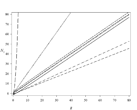
Figure 1: Comparison between the exact value (99) of $N_{0}$ (ladder), the upper limits BS$\ell$ (107) (long dash), M$\ell$ (108) (spare dot) and NUL2s (104) (short dash) and the lower limits C$\ell$ (109) (dash-dot), NLL2s (105) (solid) and NLL1 (106) (dash-dot-dot) for the M potential (96) (all with $\ell=0$ and $\alpha=1$).

The other new limits cannot be tested with this potential: the upper limit NUL1 and the limits of the second kind are not applicable because $r_{+}=\infty$, the lower limit NLL4 is only applicable to monotone potentials, and the lower limit NLL3 coincides with NLL2 for $\ell=0$.

The previously known limits applicable to this potential (note that the CMS upper limit is only applicable to monotone potentials) take the form:

$$\text{BS}\ell:\quad N_{0}\leq 2g^{2}(\alpha+\log 2+\frac{3}{2});$$ (107)

$$\text{M}\ell:\quad N_{0}\leq\sqrt{2}g(\alpha^{2}+(3-2\log 2)\alpha+1.901)^{1/4};$$ (108)

$$\text{C}\ell:\quad N_{0} > -\frac{1}{2}+\frac{2}{\pi}g\,T(\alpha),$$ (109a)

$$T(\alpha) = \max_{0\leq\gamma\leq 1}\left\{\frac{1}{\gamma}\left[\exp(\alpha)-\frac{1}{4}\exp(2\alpha)-\sqrt{1-\gamma^{2}}+\frac{\gamma^{2}}{2}\log\left(\frac{1+\sqrt{1-\gamma^{2}}}{1-\sqrt{1-\gamma^{2}}}\right)\right]\right\}.$$ (109b)

To obtain this limit we set $$a=R/(\gamma g) \ell=0 \alpha>\alpha_{0}\cong 1.386 \,\exp(\alpha_{0})=\exp(2\alpha_{0}) \ell T(\alpha) \alpha=\log 2, T(\alpha) T(\alpha)=1.055 g g \alpha \ell g) \alpha g_{\alpha} g\geq g_{\alpha} \ell \alpha=1 \ell g\geq 5.22$$ in (30) with . Note that for , with 4, this lower limit C is trivial because is then negative). Note that, for reach is maximal value: . The factor multiplying in the right-hand side of (109a) coincides which that multiplying in the right-hand side of the NLL1 lower limit (106); so for this particular value of , this C limit is slightly more stringent (of course for all values of than the NLL1 lower limit. For all other values of , there exists a value such as for all , the NLL1 limit is more stringent than the C limit. For example, for , the NLL1 limit yield more cogent results than the C limit as soon as , namely as soon as the number of bound states is greater than five.

Fig. 1 displays these limits as a function of $g$. Note that the limits depend on $\alpha$ while the exact result does not. We tested the results for the $\alpha=1$ case (not $\alpha=0,$ in oder to have a nonmonotonic potential). It is clear from this figure that the generalizations to nonmonotonic potentials of the results obtained in Ref. BC , namely the limits NUL2 and NLL2, are quite cogent. This remains true even for large values of $g:$ for instance, when the exact number $N_{0}$ of bound states is 5000, these upper and lower limits restrict its value to the rather small interval $[4996,5003]$. In this case the BS$\ell$ upper limit exceeds $1.5\ 10^{8}$, the M$\ell$ upper limit only informs us that $N<10307$, the lower limit C$\ell$ that $N>2879$ and the lower limit NLL1 that $N>3359$.

The second test is performed with the E potential (97). The exact number $N_{\ell}$ of bound states for this potential is computed by integrating numerically (191) with $\eta(0)=0$ and $\eta(\infty)=N_{\ell}\pi$, see Section III.

The upper limit NUL1$\ell$ reads

$$\text{NUL1}\ell:\quad N_{\ell}<1+\frac{2}{\pi}\sqrt{x_{+}-x_{-}}\left\{g^{2}\,\left[\exp(-x_{-})-\exp(-x_{+})\right]-\ell(\ell+1)\left(\frac{1}{x_{-}}-\frac{1}{x_{+}}\right)\right\}^{1/2},$$ (110)

where $x_{\pm}$ are the two solutions of

$$\ell(\ell+1)=g^{2}\,x_{\pm}^{2}\,\exp(-x_{\pm}).$$ (111)

The NLL1n$\ell$ limit reads

$$\text{NUL1n}\ell:\quad N_{\ell}>-1+\frac{1}{\pi}\left\{g^{2}\left[\exp(-x_{-})-\exp(-x_{+})\right]-\ell(\ell+1)\left(\frac{1}{x_{-}}-\frac{1}{x_{+}}\right)\right\}\ |V_{\ell,\text{eff}}^{\text{min}}|^{-1/2},$$ (112)

where $V_{\ell,\text{eff}}^{\text{min}}$ is the minimal value of the effective potential (24). The NUL2$\ell$ and NLL2$\ell$ limits can be written as follows:

$$\text{NUL2}\ell:\quad N_{\ell} < \frac{1}{\pi}F(g,\ell;x_{-},x_{+})+\frac{1}{2\pi}\log\left|\frac{V_{\ell,\text{eff}}^{\text{min}}}{M}\right|+1,$$ (113)

$$\text{NLL2}\ell:\quad N_{\ell} > \frac{1}{\pi}F(g,\ell;x_{-},x_{+})-\frac{1}{2\pi}\log\left|\frac{V_{\ell,\text{eff}}^{\text{min}}}{M}\right|-\frac{3}{2},$$ (114)

where

$$F(g,\ell;a,b)=\int_{a}^{b}\frac{dx}{x}\sqrt{g^{2}x^{2}\exp(-x)-\ell(\ell+1)},$$ (115)

and

$$M=\min\left[|V_{\ell,\text{eff}}(p)|,|V_{\ell,\text{eff}}(q)|\right]$$ (116a)

where $$p q$$ and are solutions of

$$F(g,\ell;x_{-},\frac{p}{R})=\frac{\pi}{2},\quad F(g,\ell;\frac{q}{R},x_{+})=\frac{\pi}{2}.$$ (116b)

The lower limits NLL3 and NLL4 take much simpler forms:

$$\text{NLL3}:\quad N_{\ell}>\frac{2}{\pi}\,g-\frac{1}{2\pi}\log\left(\frac{4g}{\pi}\right)-\frac{3}{2}-\frac{\ell}{\pi}\log\left[\frac{\log x}{\log(1-x)}\right],$$ (117)

with $x=\pi/(4g)$, and

$$\text{NLL4}:\quad N_{\ell}>\frac{2g}{\pi e(2\ell+1)}-\frac{1}{2}.$$ (118)

The previously known limits are found to be:

$$\text{BS}\ell:\quad N_{\ell}<\frac{g^{2}}{2\ell+1};$$ (119)

$$\text{CMS}:\quad N_{\ell}<\frac{4g}{\pi}+1-\sqrt{1+\frac{4\,\ell\,(\ell+1)}{\pi^{2}}};$$ (120)

$$\text{M}\ell:\quad N_{\ell}<(AB)^{1/4}$$ (121a)

where $$A B$$ and are given by

$$A = g^{2}\,\left[\exp(-x_{-})(x_{-}^{2}+2x_{-}+2)-\exp(-x_{+})(x_{+}^{2}+2x_{+}+2)\right]-\ell(\ell+1)(x_{+}-x_{-}),$$ (121b)

$$B = g^{2}\,\left[\exp(-x_{-})-\exp(-x_{+})\right]-\ell(\ell+1)\left(\frac{1}{x_{-}}-\frac{1}{x_{+}}\right);$$ (121c)

$$\text{GGMT}:\quad N_{\ell}\leq g^{2p}(2\ell+1)^{(1-2p)}\,\frac{C_{p}\Gamma(2p)}{p^{2p}},$$ (122)

with $C_{p}$ defined by (25b);

$$\text{CMS2}:\quad N_{\ell}<g^{2p}(2\ell+1)^{(1-2p)}\,\frac{\tilde{C}_{p}\Gamma(2p)}{p^{2p}},$$ (123)

with $\tilde{C}_{p}$ defined by (26b);

$$\text{C}\ell:\quad N_{\ell}>\frac{2g}{\pi(2\ell+1)}\,y\exp\left(-\frac{y}{2}\right)-\frac{1}{2},$$ (124)

where $y$ is the solution of $y\exp(-y)=(2\ell+1)y^{2\ell}\Gamma(1-2\ell,y)$.

Table 1: Comparison for the E potential (97) between the exact number $N_{\ell}$ of bound states, various upper and lower limits on $N_{\ell}$ previously known and new upper and lower limits on $N_{\ell}$, for several values of $g$ and $\ell$.

$g$	$\ell$	LLSK	NLL3	NLL1n$\ell$	NLL2$\ell$	Ex	NUL2$\ell$	BS$\ell$	CMS	M$\ell$	GGMT	NUL1$\ell$	ULSK
8	1	3	3	3	3	4	5	21	9	8	21	12	6
	3	1	1	2	1	2	3	9	8	5	6	6	4
13	2	5	4	4	5	7	8	33	15	13	31	18	9
	6	2	0	2	2	3	4	13	13	7	7	7	5
18	3	7	6	6	7	9	10	46	21	18	43	25	11
	9	2	0	3	2	4	4	17	17	9	8	9	5
24	4	10	8	8	10	12	13	64	28	24	60	33	14
	12	4	0	4	4	5	6	23	23	13	11	12	7
29	5	13	9	9	13	15	16	76	34	29	71	40	17
	15	4	0	5	4	6	7	27	28	15	13	13	8
35	6	16	11	11	16	18	19	94	41	35	88	49	20
	18	6	0	6	6	7	8	33	33	18	16	16	9
40	7	18	12	13	18	20	21	106	47	40	100	55	22
	21	6	0	6	6	8	9	37	38	20	18	18	10

Comparisons between the various limits and the exact results are presented in Table 1. The BS$\ell$ limit gives poor results when $g$ becomes large but becomes slightly better as $\ell$ grows. The CMS gives better restrictions when $\ell$ is small but behaves like the BS$\ell$ limit when $\ell$ grows. The M$\ell$ limit overestimates the number of bound states by a factor 2 when $\ell$ is small; it is no better for larger $\ell$, yet better than the BS$\ell$ and CMS limits. The GGMT limit (with, in each case, the optimized value of the parameter $p,$ see (122)) gives similar results to those yielded by the BS$\ell$ limit when $\ell$ is small and becomes better and equivalent to the M$\ell$ limit for larger values of $\ell$. The results obtained with the CMS2 limit are uninteresting hence not reported: indeed, the values of $p$ which minimize the value of the limit are either $p=1/2$ for small values of $\ell$ (in which case this limit is analogous but less stringent than the CC limit, see (29)), or $p=1$ for larger values of $\ell$ (and this yields the BS$\ell$ limit). The new limits NUL2$\ell$ and NLL2$\ell$ clearly yield the most stringent results. The NLL1n$\ell$ lower limit only yields cogent results for large values of the angular momentum. The NLL3 lower limit works reasonably well for small values of $\ell$ but becomes poor for higher values of the angular momentum. The limits of the second kind ULSK and LLSK yield similar results to those given by the NUL2$\ell$ and NLL2$\ell$ limits. Note that the arbitrary radii $r_{0}^{(\text{lo,incr)}}$ and $r_{0}^{(\text{lo,decr)}}$ have been chosen to optimize the restriction on the number of $\ell$-wave bound states. Finally, the results obtained with the C$\ell$n and the NLL4 lower limits are not reported because they are very poor. These limits give $N_{\ell}\geq 1$ for small value of $\ell$ and $N_{\ell}\geq 0$ for large value of $\ell$. This defect comes from the presence of the factor $1/(2\ell+1)$ which for instance implies that this lower bound becomes three times smaller when $\ell$ go from $0$ to $1$ while the actual number of bound states $N_{\ell}$ decreases generally only by one or two units.

The last test is performed with the Y potential (98). The exact number $N_{\ell}$ of bound states is again computed by integrating numerically (191) with $\eta(0)=0$ and $\eta(\infty)=N_{\ell}\pi$, see Section III.

The NUL1$\ell$ limit takes the form

$$\text{NUL1}\ell:\quad N_{\ell}<1+\frac{2}{\pi}\sqrt{x_{+}-x_{-}}\left\{g^{2}\int_{x_{-}}^{x_{+}}dx\frac{\exp(-x)}{x}-\ell(\ell+1)\left(\frac{1}{x_{-}}-\frac{1}{x_{+}}\right)\right\}^{1/2},$$ (125)

where $x_{\pm}$ are the two solutions of the following equation

$$\ell(\ell+1)=g^{2}\,x_{\pm}\,\exp(-x_{\pm}).$$ (126)

The NLL1n$\ell$ limit reads

$$\text{NLL1n}\ell:\quad N_{\ell}>-1+\frac{1}{\pi}\left\{g^{2}\int_{x_{-}}^{x_{+}}dx\frac{\exp(-x)}{x}-\ell(\ell+1)\left(\frac{1}{x_{-}}-\frac{1}{x_{+}}\right)\right\}\ |V_{\ell,\text{eff}}^{\text{min}}|^{-1/2},$$ (127)

where $V_{\ell,\text{eff}}^{\text{min}}$ is the minimum value of the effective potential (24). The NUL2$\ell$ and NLL2$\ell$ limits can be written as follows:

$$\text{NUL2}\ell:\quad N < \frac{1}{\pi}G(g,\ell;x_{-},x_{+})+\frac{1}{2\pi}\log\left|\frac{V_{\ell,\text{eff}}^{\text{min}}}{M}\right|+1,$$ (128)

$$\text{NLL2}\ell:\quad N > \frac{1}{\pi}G(g,\ell;x_{-},x_{+})-\frac{1}{2\pi}\log\left|\frac{V_{\ell,\text{eff}}^{\text{min}}}{M}\right|-\frac{3}{2},$$ (129)

where

$$G(g,\ell;a,b)=\int_{a}^{b}\frac{dx}{x}\sqrt{g^{2}x\exp(-x)-\ell(\ell+1)}.$$ (130)

and

$$M=\min\left[|V_{\ell,\text{eff}}(p)|,|V_{\ell,\text{eff}}(q)|\right]$$ (131a)

where $$p q$$ and are solutions of

$$G(g,\ell;x_{-},\frac{p}{R})=\frac{\pi}{2},\quad G(g,\ell;\frac{q}{R},x_{+})=\frac{\pi}{2}.$$ (131b)

The lower limits NLL3 and NLL4 take somewhat simpler forms:

$$\text{NLL3}:\quad N_{\ell}>\sqrt{\frac{2}{\pi}}\,g-\frac{x^{2}-y^{2}}{2\pi}\log\left(\frac{4g}{\pi}\right)-\frac{3}{2}-\frac{(1+4\ell)}{2\pi}\log\left(\frac{x}{y}\right),$$ (132)

where $y$ and $x$ are defined by $\text{erf}(y)=\sqrt{\pi/8}/g$, $\text{erf}(x)=1-\sqrt{\pi/8}/g$, and

$$\text{NLL4}:\quad N_{\ell}>\frac{g}{\pi\sqrt{e}(2\ell+1)}-\frac{1}{2}.$$ (133)

The previously known limits take the form:

$$\text{BS}\ell:\quad N_{\ell}<\frac{g^{2}}{2\ell+1};$$ (134)

$$\text{CMS}:\quad N_{\ell}<2\sqrt{\frac{2}{\pi}}g+1-\sqrt{1+\frac{4\,\ell\,(\ell+1)}{\pi^{2}}};$$ (135)

$$\text{M}\ell:\quad N_{\ell}<(AB)^{1/4}$$ (136a)

where $$A B$$ and are given by

$$A = g^{2}(\exp(-x_{-})(1+x_{-})-\exp(-x_{+})(1+x_{+}))-\ell(\ell+1)(x_{+}-x_{-}),$$ (136b)

$$B = g^{2}\int_{x_{-}}^{x_{+}}dx\frac{\exp(-x)}{x}-\ell(\ell+1)\left(\frac{1}{x_{-}}-\frac{1}{x_{+}}\right);$$ (136c)

$$\text{GGMT}:\quad N_{\ell}\leq g^{2p}(2\ell+1)^{(1-2p)}\,\frac{C_{p}\Gamma(p)}{p^{p}};$$ (137)

$$\text{CMS2}:\quad N_{\ell}\leq g^{2p}(2\ell+1)^{(1-2p)}\,\frac{\tilde{C}_{p}\Gamma(p)}{p^{p}};$$ (138)

$$\text{C}\ell:\quad N_{\ell}\geq\frac{2g}{\pi(2\ell+1)}\,\sqrt{y}\exp\left(-\frac{y}{2}\right)-\frac{1}{2},$$ (139)

where $y$ is the solution of $\exp(-y)=(2\ell+1)y^{2\ell}\Gamma(-2\ell,y)$.

Table 2: Comparison for the Y potential (98) between the exact number $N_{\ell}$ of bound states, various upper and lower limits on $N_{\ell}$ previously known and new upper and lower limits on $N_{\ell}$, for several values of $g$ and $\ell$.

$g$	$\ell$	LLSK	NLL3	NLL1n$\ell$	NLL2$\ell$	Ex	NUL2$\ell$	BS$\ell$	CMS	M$\ell$	GGMT	NUL1$\ell$	ULSK
8	1	3	3	2	3	5	6	21	12	8	19	16	7
	3	1	0	2	1	2	3	9	11	5	4	5	5
15	2	7	5	4	7	9	11	45	23	17	41	32	13
	6	2	0	3	2	4	5	17	20	8	8	9	8
22	3	11	8	5	11	13	15	69	33	25	64	48	17
	9	4	0	4	4	5	6	25	29	12	12	13	11
29	4	16	10	7	16	18	19	93	44	33	87	64	22
	12	5	0	5	6	7	8	33	39	16	16	18	14
35	5	19	11	8	19	21	23	111	53	40	104	76	26
	15	6	0	6	6	8	9	39	46	18	18	20	16
41	6	23	12	10	23	25	27	129	62	47	120	89	30
	18	7	0	6	7	9	10	45	54	20	20	22	18

Comparisons between the various limits and the exact results are presented in Table 2. The characteristics of the various limits for the Y potential are analogous to those commented above for the E potential. Here again the NUL2$\ell$ and the NLL2$\ell$ limits are the most effective ones, being indeed fairly stringent for all the values of $g$ and $\ell$ considered, and the limits of the second kind ULSK and LLSK also give quite stringent limits.

II.2 Tests of the limits for the value of $L$

In this subsection we test various limits on the largest value $L$ of the angular momentum quantum number $\ell$ for which the potentials E and Y do possess bound states. In this article we only obtained new lower limits on $L$. Indeed neat upper limits on $L$ cannot be extracted from the new upper limits on $N_{\ell}$ presented in Section I. But we will now see that the “naïve” upper limit $L_{\text{eff}}^{(+)}$ (63) is quite good indeed better than the previously known upper limits $L_{\text{BSL}}^{(+)}$ and $L_{\text{CMSL}}^{(+)},$ see (18) and (22).

The first test is performed with the nonsingular E potential (97). The lower limit NLL3L gives

$$L_{\text{NLL3L}}^{(-)}=\left\{\left\{\frac{\nu}{\lambda}\right\}\right\},$$ (140a)

with

$$\nu = \frac{2g}{\pi}-\frac{1}{2\pi}\log\left[\frac{1-x}{x}\right]-\frac{3}{2},$$ (140b)

$$\lambda = \frac{1}{\pi}\log\left[\frac{\log x}{\log(1-x)}\right],$$ (140c)

and $$x=\pi/(4g)$$. The lower limit NLL4L gives

$$L_{\text{NLL4L}}^{(-)}=\left\{\left\{\frac{1}{2}\left(\frac{4g}{\pi e}-1\right)\right\}\right\}.$$ (141)

The previously known upper limits on $L$ can also be obtained analytically:

$$L_{\text{BSL}}^{(+)}=\left\{\left\{\frac{1}{2}\left(g^{2}-1\right)\right\}\right\},$$ (142)

$$L_{\text{CMSL}}^{(+)}=\left\{\left\{\frac{1}{2}\left(4\,g-1\right)\right\}\right\},$$ (143)

$$L_{\text{eff}}^{(+)}=\left\{\left\{\frac{1}{2}\left(\frac{4g}{e}-1\right)\right\}\right\}.$$ (144)

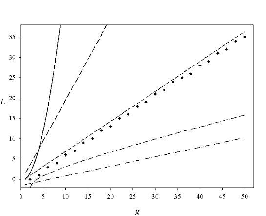
Figure 2: Comparison between the exact value of $L$ (diamond), the upper limits BSL (142) (solid), CMSL (143) (long dash) and $L_{\text{eff}}^{(+)}$ (144) (short dash) and the lower limits NLL3L (140) (dash-dot) and NLL4L (141) (dash-dot-dot) for the E potential (97).

A comparison between these limits and the exact results (computed numerically, as indicated in the preceding subsection) is presented in Fig. 2. Except for the BSL upper limit, we have the correct linear behavior in $g$ as discussed above, the best result being clearly provided by the naïve upper bound $L_{\text{eff}}^{(+)}$. Indeed this result appears hardly improvable, because the error introduced by this upper limit $L_{\text{eff}}^{(+)}$ is of at most one unit (at least for this example, as well as the following one, see below).

The second test is performed with the singular Y potential (again the exact result can only be computed numerically). The lower limit NLL3L gives

$$L_{\text{NLL3L}}^{(-)}=\left\{\left\{\frac{\nu}{\lambda}\right\}\right\},$$ (145a)

with

$$\nu = \sqrt{\frac{2}{\pi}}g-\frac{x^{2}-y^{2}}{2\pi}-\frac{1}{2\pi}\log\left[\frac{x}{y}\right]-\frac{3}{2},$$ (145b)

$$\lambda = \frac{2}{\pi}\log\left[\frac{x}{y}\right],$$ (145c)

where $$y x \text{erf}(y)=\alpha \text{erf}(x)=1-\alpha \alpha=\sqrt{(\pi/8)}/g$$ and are defined by , , . The lower limit NLL4L gives

$$L_{\text{NLL4L}}^{(-)}=\left\{\left\{-\frac{1}{2}+\frac{g}{\pi\sqrt{e}}\right\}\right\}.$$ (146)

The previously known limits on $L$ can also be obtained analytically:

$$L_{\text{BSL}}^{(+)}=\left\{\left\{\frac{1}{2}\left(g^{2}-1\right)\right\}\right\},$$ (147)

$$L_{\text{CMSL}}^{(+)}=\left\{\left\{\frac{1}{2}\left(4\sqrt{\frac{2}{\pi}}\,g-1\right)\right\}\right\},$$ (148)

$$L_{\text{eff}}^{(+)}=\left\{\left\{\frac{1}{2}\left(\frac{2g}{\sqrt{e}}-1\right)\right\}\right\}.$$ (149)

The comparison between these limits and the exact results is presented in Fig. 3. Here again, the best result is obtained from the naïve upper bound $L_{\text{eff}}^{(+)}$ for which the error is, as indicated above, of at most one unit.

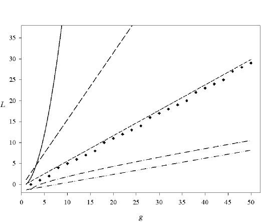
Figure 3: Comparison between the exact value of $L$ (diamond), the upper limits BSL (147) (solid), CMSL (148) (long dash) and $L_{\text{eff}}^{(+)}$ ( 149) (short dash) and the lower limits NLL3L (145) (dash-dot) and NLL4L (146) (dash-dot-dot) for the Y potential (98).

II.3 Tests of the limits for the total number of bound states $N$

This subsection is devoted to test the limits on the total number of bound states $N$. We will not test the BiS limit due to its bad behavior at large $g$. We do however test the BSN limit which yields the same incorrect behavior but is simpler to compute.

The first test is performed with the E potential (97). Again, the exact result can only be calculated numerically.

The new upper limit NUL2Nm, see (92), takes the simple form

$$N<\frac{1}{8}\left(\frac{4g}{e}+1\right)^{2}\,\left(\frac{4g}{\pi}+\frac{1}{\pi}\log\frac{4g}{\pi}+1\right).$$ (150)

The new lower limit NLLN3 reads

$$N>\frac{\nu}{6}\left(2\left(L_{\text{NLL3L}}^{(-)}\right)^{2}+7L_{\text{NLL3L}}^{(-)}+6\right),$$ (151)

with $L_{\text{NLL3L}}^{(-)}$ and $\nu$ given by equations (140a) and (140b); and the new lower limit NLLN4 is given by (95) with $\sigma=4\,g/(e\,\pi)$.

The other, previously known limits read as follows:

$$\text{BSN}:\quad N<\frac{1}{2}g^{2}(g^{2}+1),$$ (152)

$$\text{Lcentral}:\quad N<0.864\,g^{3},$$ (153)

$$\text{CMSN}:\quad N<1.698\,(g^{3}+2.3562\,g^{2}+1.116\,g+0.1473).$$ (154)

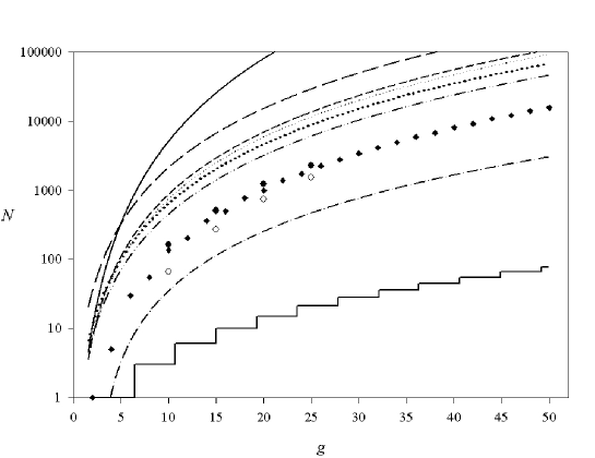
Figure 4: Comparison between the exact value of $N$ (diamond), the upper limits BSN (152) (solid), CMSN (154) (long dash), Lcentral (153) (short dash), improved BSN (155) (dot), improved CMSN (156) (sparse dot), NUL2Nm (150) (dash dot dot) and the lower limits NLLN3 (151) (dash dot) and NLLN4 (95) (ladder) for the E potential (97). The black and the white circles correspond respectively to the NUL2N and NLL2N limits.

The BSN and the CMSN limits can be improved: instead of using the limit on $L$ provided by these limits ($L_{\text{BSL}}^{(+)}$ and $L_{\text{CMSL}}^{(+)}$), we can use the best upper limits $L_{\text{eff}}^{(+)}$ (63); the BSN and CMSN limits obtained in this manner are called here improved BSN and CMSN limits:

$$\text{{improved} BSN:}\quad N<\frac{1}{2}g^{2}\left(\frac{4g}{e}+1\right)$$ (155)

$$\text{{improved} CMSN:}\quad N<0.5202\,(g^{3}+2.179\,g^{2}+1.726\,g+0.4806)$$ (156)

Fig. 4 presents a comparison between the various limits and the exact result. It shows that the limits on the total number of bound states which can be expressed in a neat form are not very stringent. [Indeed, the best results are yielded by the upper limit NUL2Nn which is obtained using only a limit on the number of S-wave bound states, $N_{0}$, and the simple limit $L_{\text{eff}}^{(+)}$ on the maximal value $L$ of $\ell$ for which bound states do exist]. There are at least three reasons for this. First, most of the limits do not contain the appropriate functional of the potential (as identified by the asymptotic behavior at large $g$ of $N,$ see (16b)): only the Lieb limit Lcentral, see (89), features the correct form, but the numerical factor is not optimal indeed too large (by approximately a factor 7). The second reason is that for every value of $\ell$, there is a round-off error introduced by the limit; to obtain the limit on the total number of bound states we sum all these errors. The third reason is that to be able to make the summation over the values of $\ell$ we must have an explicit dependence of the limits on $\ell$, and this entails that we cannot use some of the limits we found; in particular we cannot use the new upper and lower limits NUL2 and the NLL2, which are quite stringent, to obtain a neat formula. But we can use them and compute upper and lower limits on $N_{\ell}$, then sum all these contributions to obtain upper and lower limits on $N$, the sum being stopped when $N_{\ell}^{(+)}$ is smaller than 1 and $N_{\ell}^{(-)}$ is negative (see subsection I.6). We call NUL2N respectively NLL2N the upper respectively lower limits on the total number of bound states $N$ obtained (from NUL2 respectively NLL2) via this (inelegant) procedure. Fig. 4 shows, for 4 values of $g$, that these limits are quite stringent.

The second test is performed with the Y potential. Again, the exact total number of bound states is computed numerically, as indicated above.

The new upper limit NUL2Nm, see (92) reads

$$\text{NUL2Nm:}\quad N<\frac{1}{8}\left(\frac{2g}{\sqrt{e}}+1\right)^{2}\,\left(2g\sqrt{\frac{2}{\pi}}+\frac{x^{2}-y^{2}}{\pi}+\frac{1}{\pi}\log\frac{x}{y}+1\right),$$ (157)

where $y$ and $x$ are defined by $\text{erf}(y)=\sqrt{\pi/8}/g$, $\text{erf}(x)=1-\sqrt{\pi/8}/g$. The new limits NLLN3 and NLLN4 are:

$$\text{NLLN3:}\quad N>\frac{\nu}{6}\left(2\left(L_{\text{NLL3L}}^{(-)}\right)^{2}+7L_{\text{NLL3L}}^{(-)}+6\right),$$ (158)

with $L_{\text{NLL3L}}^{(-)}$ and $\nu$ given by equations (145) and (145b); while the lower limit NLLN4 is given by (95) with $\sigma=2\,g/(\sqrt{e}\pi)$.

The other previously known limits read:

$$\text{BSN}:\quad N<\frac{1}{2}g^{2}(g^{2}+1),$$ (159)

$$\text{Lcentral}:\quad N<0.703\,g^{3},$$ (160)

$$\text{CMSN}:\quad N<3.3422\,(g^{3}+1.88\,g^{2}+0.711\,g+0.075).$$ (161)

$$\text{{improved} BSN:}\quad N<\frac{1}{2}g^{2}\left(\frac{2g}{\sqrt{e}}+1\right)$$ (162)

$$\text{{improved} CMSN:}\quad N<0.4924\,(g^{3}+2.237\,g^{2}+1.781\,g+0.5078)$$ (163)

A comparison between the various limits and the exact numerical results is presented in Fig. 5, in analogy to the case of the E potential and with analogous conclusions, see above.

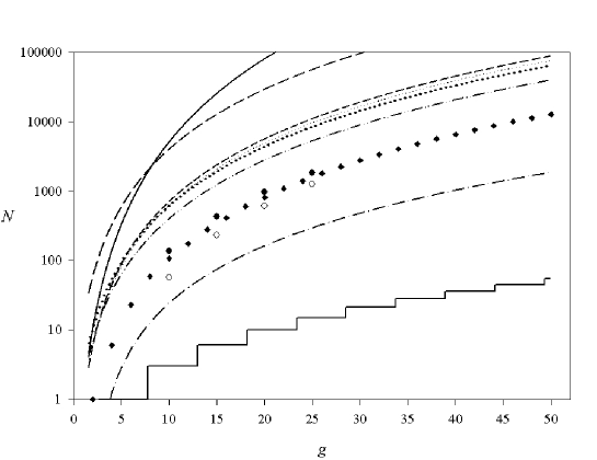
Figure 5: Comparison between the exact value of $N$ (diamond), the upper limits BSN (159) (solid), CMSN (161) (long dash), Lcentral (160) (short dash), improved BSN (162) (dot) and improved CMSN (163) (sparse dot), NUL2Nm (157) (dash dot dot) and the lower limits NLLN3 (158) (dash dot) and NLLN4 (95) (ladder) for the Y potential (98). The black and the white circles correspond respectively to the NUL2N and NLL2N limits.

III PROOFS

In this section we prove the new results reported in Section I. Because we tried and presented those results in Section I in a user-friendly order, the proofs given below do not follow the same order, due to the need here to follow a more logical sequence. To provide some guidance we divided this section into several subsections, but we must forewarn the reader that a sequential reading is essential to understand what goes on.

III.1 Tools

The starting point of our treatment is the well-known fact (see Section I) that the number $N_{\ell}$ of ($\ell$-wave) bound states possessed by the potential $V(r)$ coincides with the number of zeros, in the interval $0<r<\infty,$ of the function $u(r)$ uniquely defined (up to an irrelevant multiplicative constant) as the solution of the zero-energy $\ell$-wave radial Schrödinger equation

$$u^{\prime\prime}(r)=\left[V(r)+\frac{\ell(\ell+1)}{r^{2}}\right]\,u(r)$$ (164a)

with the boundary condition

$$u(0)=0.$$ (164b)

To get an efficient handle on the task of counting these zeros (or rather, of providing upper and lower limits on their number) it is convenient to introduce a new dependent variable $\eta(r)$ related to $u(r)$ as follows:

$$\left[-U(r)\right]^{1/2}\cot\left[\eta(r)\right]=f(r)+\frac{u^{\prime}(r)}{u(r)}.$$ (165)

Here we moreover introduce two new functions: a function $f(r)$, which we reserve to assign at our convenience below with the only proviso that it be finite in the open interval $0<r<\infty$, and nonnegative throughout this interval,

$$f(r)\geq 0\quad\text{for}\quad 0\leq r<\infty;$$ (166)

and a function $U(r),$ which might or might not coincide with the potential $V(r)$ (see below) but that (unless we explicitly state otherwise) we require to be finite in the open interval $0<r<\infty$ , to satisfy (at least) the properties (see (2), (3) and (4))

$$-U(r)=\left|U(r)\right|,$$ (167)

$$\underset{r\rightarrow\infty}{\lim}\left[r^{2+\varepsilon}U(r)\right]=0,$$ (168)

$$\underset{r\rightarrow 0}{\lim}\left[r^{2-\varepsilon}U(r)\right]=0,$$ (169)

and to be related to the potential $V(r)$ as follows:

$$U(r)+W(r)=V(r)+\frac{\ell(\ell+1)}{r^{2}},$$ (170)

where we still reserve the privilege to assign the function $W(r)$ at our convenience (a possibility will be to set $U(r)=V(r)$ hence $W(r)=\ell(\ell+1)/r^{2}$; but it shall not be the only one, see below). Of course the function $\eta(r)$ (as well as $u(r)$) depends on $\ell$, although for notational simplicity we omit to indicate this explicitly, and this remark may as well apply to the other functions, $f(r),$ $U(r),$ $W(r)$, introduced here and utilized below.

It is then easy to see that the function $\eta(r)$ is uniquely characterized by the first-order nonlinear ODE (implied by (165) with (170), and (164a))

$$\eta^{\prime}(r) = \left|U(r)\right|^{1/2}+\left|U(r)\right|^{-1/2}\left\{\left[f(r)\right]^{2}-f^{\prime}(r)-W(r)\right\}\sin^{2}\left[\eta(r)\right]$$ (171)

$$-\left\{\left[4\left|U(r)\right|\right]^{-1}\,U^{\prime}(r)+f(r)\right\}\sin\left[2\eta(r)\right],$$

with the boundary condition (implied by (165) with (164b) and (169))

$$\eta(0)=0.$$ (172)

We of course assume the function $\eta(r)$ to be continuous, disposing thereby of the $\text{mod}(\pi)$ ambiguity entailed by the definition (165).

It is now easy to see that this function $\eta(r)$ provides a convenient tool to evaluate the number of zeros $N_{\ell}$ of $u(r)$. Indeed, if we denote with $z_{n}$ the zeros of $u(r),$ $u(z_{n})=0$, ordered so that

$$0\equiv z_{0}<z_{1}<\ldots<z_{N_{\ell}}$$ (173)

(see Section I), since clearly (see (171)) whenever $\eta(r)$ is an integer multiple of $\pi$ the derivative $\eta^{\prime}(r)$ is nonnegative, $\eta^{\prime}(r)\geq 0$, we may conclude (see (165)) that

$$\eta(z_{n})=n\pi,\quad n=0,1,\ldots,N_{\ell},$$ (174)

with

$$(n-1)\pi\leq\eta(r)\leq n\pi\quad\text{for}\quad z_{n-1}\leq r\leq z_{n},\ n=1,\ldots,N_{\ell}.$$ (175)

It is moreover plain that, provided (see (165))

$$\underset{r\rightarrow\infty}{\lim}\left[\frac{\left|U(r)\right|^{1/2}}{f(r)+\frac{u^{\prime}(r)}{u(r)}}\right]=0,$$ (176)

there holds the asymptotic relation

$$\eta(\infty)=N_{\ell}\pi,$$ (177)

and that this asymptotic value is approached from above. [To prove the last statement one sets, in the asymptotic large $r$ region, $\eta(r)=N_{\ell}\pi+\varepsilon(r)$ with $\left|\varepsilon(r)\right|\ll 1$, and uses the asymptotic estimates $\sin^{2}(N_{\ell}\pi+\varepsilon)\approx\varepsilon^{2},$ $\sin\left[2(N_{\ell}\pi+\varepsilon)\right]\approx 2\varepsilon$ to rewrite the ODE (171) in the asymptotic region as follows (recall that $U(r)$ is nonpositive, see (167)):

$$\varepsilon^{\prime}(r)\approx\left[-U(r)\right]^{1/2}+\left\{\frac{U^{\prime}(r)}{2\,U(r)}-2\,f(r)\right\}\varepsilon(r).$$ (178)

One can then replace the approximate equality sign $\approx$ in this formula with the equality sign = and integrate the resulting linear ODE, obtaining

$$\varepsilon(r)=\left|U(r)\right|^{1/2}\int_{R}^{r}dx\,\exp\left[2\int_{r}^{x}dy\,f(y)\right],$$ (179)

where $R$ is a (finite) integration constant, and this formula (valid in the asymptotic, large $r$, region, where of course $r>R$) shows that $\varepsilon(r)$ is indeed positive].

To get a more detailed information on the behavior of the function $\eta(r)$ we make the additional assumption that the assignments of the auxiliary functions $f(r)$ and $W(r)$ guarantee validity of the following inequality:

$$\left[f(r)\right]^{2}-f^{\prime}(r)-W(r)\geq 0$$ (180)

(it would be enough for our purposes that this inequality be valid only at large values of $r$ – but for simplicity we assume hereafter its validity for all values of $r,$ $0\leq r<\infty$). It is then clear from the ODE (171) satisfied by $\eta(r)$ that, wherever $\eta(r)$ takes a value which is an odd integer multiple of $\pi/2$, namely at the points $r=b_{n}$ such that

$$\eta(b_{n})=\frac{1}{2}(2n-1)\pi,\quad n=1,2,\ldots,N_{\ell},$$ (181)

its derivative $\eta^{\prime}(r)$ is nonnegative, $\eta^{\prime}(b_{n})\geq 0$. Hence we may complement the information provided by (174) with that provided by this formula, (181), and moreover replace the information provided by (175) with the following more detailed information:

$$(n-1)\pi\leq\eta(r)\leq\frac{1}{2}(2n-1)\pi\quad\text{for}\quad z_{n-1}\leq r\leq b_{n},\ n=1,\ldots,N_{\ell},$$ (182)

$$(2n-1)\frac{\pi}{2}\leq\eta(r)\leq n\pi\quad\text{for}\quad b_{n}\leq r\leq z_{n},\ n=1,\ldots,N_{\ell},$$ (183)

which of course also entails that the points $z_{n}$ and $b_{n}$ are interlaced,

$$z_{0}<b_{1}<z_{1}<b_{2}<\ldots<z_{N_{\ell}-1}<b_{N_{\ell}}<z_{N_{\ell}}<\infty.$$ (184)

And note in particular that these formulas entail the following important inequality (implied by the non existence of $b_{N_{\ell}+1}$), valid for all values of $r,$ $0\leq r<\infty$:

$$0\leq\eta(r)<\left(N_{\ell}+\frac{1}{2}\right)\pi.$$ (185)

It is moreover clear that the maximum value of $\eta(r)$,

$$\hat{\eta}=\underset{0\leq r<\infty}{\max}\left[\eta(r)\right],$$ (186)

is actually attained in the interval $z_{N_{\ell}}<r<\infty$, and that it lies in the range

$$N_{\ell}\,\pi\leq\hat{\eta}<\left(N_{\ell}+\frac{1}{2}\right)\,\pi.$$ (187)

We are now in the position to derive the new upper and lower limits reported in Section I.

III.2 Proof of the lower limits NLL4

We begin by proving the lower limit NLL4, see (61). To this end we assign as follows the functions $f(r)$ and $W(r)$:

$$f(r)=\frac{\ell}{r},\quad W(r)=\frac{\ell(\ell+1)}{r^{2}},$$ (188)

entailing that the left-hand side of the inequality (180) vanishes, that

$$U(r)=V(r),$$ (189)

that the definition (165) now reads

$$\left|V(r)\right|^{1/2}\,\cot\left[\eta(r)\right]=\frac{\ell}{r}+\frac{u^{\prime}(r)}{u(r)},$$ (190)

and, most importantly, that (171) reads

$$\eta^{\prime}(r)=\left|V(r)\right|^{1/2}-\left\{\frac{V^{\prime}(r)}{4\left|V(r)\right|}\,+\frac{\ell}{r}\right\}\sin\left[2\eta(r)\right].$$ (191)

Here we are of course assuming the potential $V(r)$ to satisfy the condition (2).

Before proceeding with the proof, let us note that, for the potential (34), the second term in the right-hand side of this ODE, (191), vanishes, hence one immediately obtains

$$\eta(r)=\frac{g}{2\ell+1}\min\left[\alpha^{2\ell+1},\left(\frac{r}{R}\right)^{2\ell+1}\right].$$ (192)

Hence (see (177)), for the potential (34),

$$N_{\ell}=\left\{\left\{\frac{g\,\alpha^{2\ell+1}}{\pi(2\ell+1)}\right\}\right\},$$ (193)

where as usual the double braces signify that the integral part must be taken of their contents. This observation implies that the upper and lower limits which obtain (see below) by massaging the last term in the right-hand side of the ODE (191) are generally best possible, being saturated by the potential (34) (if need be, with an appropriate choice of the parameter $\alpha$, see Section I).

To prove (61) with (8) we now introduce the auxiliary function $\eta_{\text{lo}}(r)$ via the ODE

$$\eta_{\text{lo}}^{\prime}(r)=\left|V(r)\right|^{1/2}-\left\{\frac{V^{\prime}(r)}{2\left|V(r)\right|}\,+\frac{2\ell}{r}\right\}\eta_{\text{lo}}(r)$$ (194)

with the boundary condition

$$\eta_{\text{lo}}(0)=0.$$ (195)

We then assume the potential $V(r)$ to satisfy, in addition to (2), the condition (5). It is then plain (see (191) with (172), (194) with (195), and (5)) that, for all values of $r,$ $0\leq r<\infty$,

$$\eta_{\text{lo}}(r)\leq\eta(r).$$ (196)

[Indeed (194) obtains from (191) via the replacement $\sin(x)\Rightarrow x,$ and for positive $x$, $\sin(x)\leq x$; hence $\eta_{\text{lo}}(r)$ can never overtake $\eta(r)$ because, at the overtaking point, a comparison of (194) with (191) entails $\eta_{\text{lo}}^{\prime}(r)\leq\eta^{\prime}(r)$, which negates the possibility to perform the overtaking]. But the linear ODE (194) with (195) can be easily integrated to yield (recalling (2))

$$\eta_{\text{lo}}(r)=\frac{r\,\left|V(r)\right|^{1/2}}{2\ell+1},$$ (197)

hence we conclude (see (186), (196), (197) and (8)) that

$$\hat{\eta}\geq\frac{\pi\sigma}{2(2\ell+1)},$$ (198)

and via (187) this entails the lower limit NLL4, see (61), which is thereby proven.

III.3 Proof of the upper and lower limits NUL2 and NLL2

Let us now prove the upper and lower limits NUL2 and NLL2, see (44) and (45), on the number $N_{0}$ of S-wave bound states possessed by the central potential $V(r)$, of course under the assumption that this potential satisfy the conditions (43). The main tool of the proof is the same function $\eta(r)$ as defined in the preceding subsection III.2, which is therefore now defined by the formula (see (190))

$$\left|V(r)\right|^{1/2}\,\cot\left[\eta(r)\right]=\frac{u^{\prime}(r)}{u(r)},$$ (199)

and satisfies the ODE (see (191))

$$\eta^{\prime}(r)=\left|V(r)\right|^{1/2}-\frac{V^{\prime}(r)}{4\left|V(r)\right|}\,\sin\left[2\eta(r)\right].$$ (200)

Note that this is just the function $\eta(r)$ that provided our main analytical tool in BC ; however the conditions (43a) and (43b) (which clearly imply $V(r_{-})=0$) entail now, via (199), the condition

$$\eta(r_{-})=0,$$ (201)

as well as the fact that $u(r)$ is concave in the interval $0\leq r\leq r_{-}$ (see (164a) and (43a)), hence it has no zero in that interval, hence

$$r_{-}<b_{1}<z_{1}$$ (202)

(see (174), (181) and (199)). Likewise the fact that $u(r)$ is also concave in the interval $r_{+}\leq r<\infty$ (see (164a) and (43d)), hence it has no extremum in that interval, entails

$$z_{N_{0}-1}<b_{N_{0}}<r_{+}.$$ (203)

To obtain the upper limit NUL2 we now integrate the ODE (200) from $z_{1}$ to $z_{N_{0}-1}$ (and note that, thanks to (202) and (203), as well as (43), we can hereafter replace, whenever convenient, $\left|V(r)\right|$ with $-V^{(-)}(r)$, see (9)):

$$\eta(z_{N_{0}-1})-\eta(z_{1}) = (N_{0}-2)\,\pi=\int_{z_{1}}^{z_{N_{0}-1}}dr\,\left[-V^{(-)}(r)\right]^{1/2}-\frac{1}{4}\int_{z_{1}}^{r_{\text{min}}}dr\,\frac{V^{\prime}(r)}{\left|V(r)\right|}\,\sin\left[2\eta(r)\right]$$ (204)

$$-\frac{1}{4}\int_{r_{\text{min}}}^{z_{N_{0}-1}}dr\,\frac{V^{\prime}(r)}{\left|V(r)\right|}\,\sin\left[2\eta(r)\right].$$

The first equality is of course entailed by (174). As for the second equation, note that we conveniently split the integration of the second term in the right-hand side of (200) in two parts. The properties (43b), (43c) (as well as the obvious fact that $\left|\sin(x)\right|\leq 1$), allow us to majorize the right-hand side of this equation, (204). We thereby get

$$\left(N_{0}-2\right)\,\pi<\int_{z_{1}}^{z_{N_{0}-1}}dr\,\left[-V^{(-)}(r)\right]^{1/2}+\frac{1}{4}\int_{z_{1}}^{r_{\text{min}}}dr\,\frac{V^{\prime}(r)}{V(r)}-\frac{1}{4}\int_{r_{\text{min}}}^{z_{N_{0}-1}}dr\,\frac{V^{\prime}(r)}{V(r)},$$ (205)

hence,

$$\left(N_{0}-2\right)\,\pi<\int_{z_{1}}^{z_{N_{0}-1}}dr\,\left[-V^{(-)}(r)\right]^{1/2}+\frac{1}{4}\,\log\left\{\frac{\left[V^{(-)}(r_{\text{min}})\right]^{2}}{V^{(-)}(z_{1})\,V^{(-)}(z_{N_{0}-1})}\right\}.$$ (206)

We now need to find quantities $p$ and $q$, defined only in terms of the potential, such that $p\leq z_{1}$ and $q\geq z_{N_{0}-1}$ and also such that $\left|V(p)\right|\leq\left|V(z_{1})\right|$ and $\left|V(q)\right|\leq\left|V(z_{N_{0}-1})\right|$. Let us first consider the “favorable” case (which obtains for a sufficiently attractive potential): $z_{1}\leq r_{\text{min}}$ and $z_{N_{0}-1}\geq r_{\text{min}}$. In this case, we integrate (200) from $b_{1}$ to $z_{1}$ and since in this interval both $V^{\prime}(r)/\left|V(r)\right|$ and $\sin\left[2\eta(r)\right]$ are negative, we infer

$$\eta(z_{1})-\eta(b_{1})=\frac{\pi}{2}\leq\int_{b_{1}}^{z_{1}}dr\,\left[-V^{(-)}(r)\right]^{1/2},$$ (207)

hence a fortiori (see (202))

$$\int_{0}^{z_{1}}dr\,\left[-V^{(-)}(r)\right]^{1/2}>\frac{\pi}{2}.$$ (208)

If we define $p$ via the formula

$$\int_{0}^{p}dr\,\left[-V^{(-)}(r)\right]^{1/2}=\frac{\pi}{2},$$ (209)

then we conclude (by comparing (208) with (209)) that $p<z_{1}$. Moreover, since we have supposed $z_{1}\leq r_{\text{min}}$, we have also $\left|V(p)\right|<\left|V(z_{1})\right|$. We then integrate (200) from $z_{N_{0}-1}$ to $b_{N_{0}},$ and taking advantage of the fact that in this interval both $V^{\prime}(r)/\left|V(r)\right|$ and $\sin\left[2\,\eta(r)\right]$ are positive, we infer

$$\eta(b_{N_{0}})-\eta(z_{N_{0}-1})=\frac{\pi}{2}\leq\int_{z_{N_{0}-1}}^{b_{N_{0}}}dr\,\left[-V^{(-)}(r)\right]^{1/2},$$ (210)

hence a fortiori (see (203))

$$\frac{\pi}{2}<\int_{z_{N_{0}-1}}^{\infty}dr\,\left[-V^{(-)}(r)\right]^{1/2}.$$ (211)

Analogously, if we define $q$ via the formula

$$\int_{q}^{\infty}dr\,\left[-V^{(-)}(r)\right]^{1/2}=\frac{\pi}{2},$$ (212)

we conclude that $q>z_{N_{0}-1}$. Moreover, since we have supposed $z_{N_{0}-1}\geq r_{\text{min}}$, we have also $\left|V(q)\right|<\left|V(z_{N_{0}-1})\right|$. Thus if these two relations, $z_{1}\leq r_{\text{min}}$ and $z_{N_{0}-1}\geq r_{\text{min}},$ hold, we obtain

$$N_{0}<\frac{1}{\pi}\int\nolimits_{0}^{\infty}dr\,\left[-V^{(-)}(r)\right]^{1/2}+\frac{1}{4\pi}\log\left\{\frac{\left[V^{(-)}(r_{\text{min}})\right]^{2}}{V^{(-)}(p)V^{(-)}(q)}\right\}+1,$$ (213)

where we have used the equations (209) and (212). This last relation imply the validity of the relation (44).

We need now to consider the cases where $z_{1}>r_{\text{min}}$ or $z_{N-1}<r_{\text{min}}$. In these cases we could have, for example, $p<z_{1}$ and $\left|V(p)\right|>\left|V(z_{1})\right|$.

Firstly, suppose $z_{1}>r_{\text{min}}$ which implies that $z_{N_{0}-1}>r_{\text{min}}$. Now we impose a first condition for the applicability of the limit NUL2: $p\leq r_{\text{min}}$. This condition is always true for a potential which possesses enough bound states; in practice, the limit NUL2 will be applicable only when the attractive strength of the potential is large enough. This condition ensures that $p<z_{1}$ (this is not necessarily true, with the definition (209), when $z_{1}>r_{\text{min}}$). Indeed, if $z_{1}\leq r_{\text{min}}$, we have proved it above, and if $z_{1}>r_{\text{min}}$, this is still true since $p\leq r_{\text{min}}$. Moreover, since $z_{1}>r_{\text{min}}$, we have $\left|V(z_{1})\right|>\left|V(z_{N_{0}-1})\right|>\left|V(q)\right|\geq M$, with

$$M=\min(\left|V(p)\right|,\left|V(q)\right|)=\min\left[-V^{(-)}(p),-V^{(-)}(q)\right].$$ (214)

This implies the validity of the relation (44).

Secondly, suppose $z_{N_{0}-1}<r_{\text{min}}$ which obviously implies $z_{1}<r_{\text{min}}$. Now we impose a second condition for the applicability of the limit: $q\geq r_{\text{min}}$. This condition is always true for a potential which possesses enough bound states. This condition ensure that $q>z_{N_{0}-1}$ (this is not necessarily true, with the definition (212), when $z_{N_{0}-1}<r_{\text{min}}$). Indeed, if $z_{N_{0}-1}\geq r_{\text{min}}$, we have proved it above, and if $z_{N_{0}-1}<r_{\text{min}}$, this is still true since $q\geq r_{\text{min}}$. Moreover, since $z_{N_{0}-1}<r_{\text{min}}$, we have $\left|V(z_{N_{0}-1})\right|>\left|V(z_{1})\right|>\left|V(p)\right|\geq M$, with $M$ defined again by (214). This implies, via the definitions (7) and (9), the validity of the relation (44), and concludes our proof of the new upper limit NUL2.

The proof of the new lower limit NLL2, see (45), is completely analogous, except that one integrates the ODE (200) from $p$ to $q$

$$\eta(q)-\eta(p)\geq\int_{p}^{q}dr\,\left[-V^{(-)}(r)\right]^{1/2}-\frac{1}{4}\int_{p}^{r_{\text{min}}}dr\,\frac{V^{\prime}(r)}{V(r)}+\frac{1}{4}\int_{r_{\text{min}}}^{q}dr\,\frac{V^{\prime}(r)}{V(r)},$$ (215)

and from the inequalities (actually valid for any positive radius, see (185))

$$\eta(p)\geq 0,$$ (216)

$$\eta(q)<\left(N_{0}+\frac{1}{2}\right)\,\pi,$$ (217)

we clearly infer

$$\eta(q)-\eta(p)<\left(N_{0}+\frac{1}{2}\right)\,\pi.$$ (218)

Hence

$$\left(N_{0}+\frac{1}{2}\right)\,\pi>\int_{p}^{q}dr\,\left[-V^{(-)}(r)\right]^{1/2}-\frac{1}{4}\int_{p}^{r_{\text{min}}}dr\,\frac{V^{\prime}(r)}{V(r)}+\frac{1}{4}\int_{r_{\text{min}}}^{q}dr\,\frac{V^{\prime}(r)}{V(r)},$$ (219)

hence, via the definitions (209) and (212) of $p$ and $q$,

$$\left(N_{0}+\frac{3}{2}\right)\,\pi>\int_{0}^{\infty}dr\,\left[-V^{(-)}(r)\right]^{1/2}-\frac{1}{4}\,\log\left\{\frac{\left[V^{(-)}(r_{\text{min}})\right]^{2}}{V^{(-)}(p)\,V^{(-)}(q)}\right\}.$$ (220)

Note that this inequality is true in any case, provided $p\leq r_{\text{min}}\leq q$, and of course it implies (again, via the definitions (7) and (9), as well as (214)) the validity of the marginally less stringent lower bound (45) (we preferred to display in Section I the lower bound (45) rather than the more stringent one implied by (220) to underline its analogy with the upper bound (44)).

III.4 Proof of the lower limits NLL3s and NLL3

Let us now proceed and prove (following BC ) the new lower limits NLL3s and NLL3, see (57) and (59). The proof is analogous to the proofs of the NUL2 and NLL2 limits given in the previous subsection except that now instead of considering the equation (200) for $\eta(r)$ we use the equation (191). To obtain NLL3s, we integrate the ODE (191) from $p$ to an arbitrary radius $s\geq r_{\text{min}}$:

$$\eta(s)-\eta(p) = \int_{p}^{s}dr\,\left[-V^{(-)}(r)\right]^{1/2}-\frac{1}{4}\int_{p}^{r_{\text{min}}}dr\,\frac{V^{\prime}(r)}{\left|V(r)\right|}\,\sin\left[2\eta(r)\right]$$ (221)

$$-\frac{1}{4}\int_{r_{\text{min}}}^{s}dr\,\frac{V^{\prime}(r)}{\left|V(r)\right|}\,\sin\left[2\eta(r)\right]-\int\nolimits_{p}^{s}dr\,\frac{\ell}{r}\,\sin\left[2\eta(r)\right].$$

The right-hand side of this last equation can be minorized (since $\eta(s)<(N_{\ell}+1/2)\pi$ and $\eta(p)>0$, see (185)) to yield

$$\left(N_{\ell}+\frac{1}{2}\right)\,\pi>\eta(s)-\eta(p)\geq\int_{p}^{s}dr\,\left[-V^{(-)}(r)\right]^{1/2}-\frac{1}{4}\int_{p}^{r_{\text{min}}}dr\,\frac{V^{\prime}(r)}{V(r)}+\frac{1}{4}\int_{r_{\text{min}}}^{s}dr\,\frac{V^{\prime}(r)}{V(r)}-\ell\,\log\left(\frac{s}{p}\right).$$ (222)

From the definition of $p$, see (47), we finally obtain

$$\left(N_{\ell}+1\right)\pi>\int_{0}^{s}dr\,\left[-V^{(-)}(r)\right]^{1/2}-\frac{1}{4}\log\left\{\frac{\left[V^{(-)}(r_{\text{min}})\right]^{2}}{V^{(-)}(p)V^{(-)}(s)}\right\}-\ell\log\left(\frac{s}{p}\right),$$ (223)

which coincides with the lower limit NLL3s, see (57), that is thereby proven.

To get the lower limit NLL3 we proceed as above, except that we integrate from $p$ to $q,$ see (47) and (48).

III.5 Proof of the results in terms of comparison potentials (see Section I.4)

Let us now prove the relations (65) and (66). We assume for this purpose that the potential $V(r)$ satisfy the negativity condition (2), but we require no monotonicity condition on $V(r)$; we do however require the potential $V(r)$ to be nonsingular for $0\leq r<\infty$ and to satisfy the conditions, see (3) and (4), that are sufficient to guarantee that the quantity $S$, see (7), be finite.

Let us now replace the potential $V(r)$ with $V(r)+H_{\lambda}^{(\ell)}(r)$, so that the radial Schrödinger equation, see (164a), read now

$$u^{\prime\prime}(r)=\left[V(r)+H_{\lambda}^{(\ell)}(r)+\frac{\ell\,(\ell+1)}{r^{2}}\right]\,u(r)$$ (224)

and the relation (170) read now

$$U(r)+W(r)=V(r)+H_{\lambda}^{(\ell)}(r)+\frac{\ell\,(\ell+1)}{r^{2}}.$$ (225)

Let us moreover set (see (165))

$$U(r)=V(r),$$ (226)

$$f(r)=\frac{V^{\prime}(r)}{4V(r)},$$ (227)

so that (see (225))

$$W(r)=H_{\lambda}^{(\ell)}(r)+\frac{\ell\,(\ell+1)}{r^{2}},$$ (228)

with the additional requirement

$$H_{\lambda}^{(\ell)}(r)+\frac{\ell(\ell+1)}{r^{2}}-\left[f(r)\right]^{2}+f^{\prime}(r)=\beta\,\left|V(r)\right|,$$ (229)

where $\beta<1$. [Note that we imposed in (180) that the left-hand side of (229) be positive. Actually this restriction, which was introduced to prove that $\eta^{\prime}(b_{n})\geq 0$ (see (181)), was too strong for our needs. Indeed, one can verify from (171) that we still have $\eta^{\prime}(b_{n})\geq 0$ provided $\beta<1$]. It is easily seen that this entails for $H_{\lambda}^{(\ell)}(r)$ the definition (64) via the assignment

$$\beta=1-4\lambda^{2}.$$ (230)

Hence these assignments imply that the definition of $\eta(r),$ see (165), reads now

$$\left[-V(r)\right]^{1/2}\cot\left[\eta(r)\right]=\frac{V^{\prime}(r)}{4\,V(r)}+\frac{u^{\prime}(r)}{u(r)},$$ (231)

and, most importantly, that the equation (171) satisfied by $\eta(r)$ becomes now simply

$$\eta^{\prime}(r)=\left|V(r)\right|^{1/2}\left\{1-\beta\,\sin^{2}\left[\eta(r)\right]\right\},$$ (232)

entailing

$$\eta^{\prime}(r)\left\{1-\beta\,\sin^{2}\left[\eta(r)\right]\right\}^{-1}=\left|V(r)\right|^{1/2}.$$ (233)

Both sides of this last equation are now easily integrated, the right-hand side from $r=0$ to $r=\infty,$ and the left-hand side, correspondingly, from $\eta=0$ (see (172), which is clearly implied by (231) and by (164b)) to $\eta(\infty)$, yielding (see (7) and (230))

$$\eta(\infty)=\,\lambda\,S\,\pi.$$ (234)

It is on the other hand clear that in this case as well

$$N_{\ell}\,\pi\leq\eta(\infty)<(N_{\ell}+1)\,\pi.$$ (235)

[Indeed, while in this case the relation (176) does not hold and therefore neither (177) nor (187) need be true, the relation (174) is still implied by the definition (231), and moreover (233) clearly implies $\eta^{\prime}(z_{n})\geq 0,$ entailing validity of these inequalities]. Hence (see (234))

$$N_{\ell}^{(V+H_{\lambda}^{(\ell)})}=\left\{\left\{\lambda\,S\right\}\right\}\,,$$ (236)

where as usual the double brace denote the integer part. In this last formula the notation $N_{\ell}^{(V+H_{\lambda}^{(\ell)})}$ denotes of course the number of $\ell$-wave bound states possessed by the potential $V(r)+H_{\lambda}^{(\ell)}(r).$

But if the “additional potential” $H_{\lambda}^{(\ell)}(r)$, see (64), is nowhere negative, this potential $V(r)+H_{\lambda}^{(\ell)}(r)$ cannot possess less ($\ell$-wave) bound states than the potential $V(r)$, hence the lower limit (65) is proved. And under the same conditions, if the function $H_{\lambda}^{(\ell)}(r)$ is nowhere positive, the potential $V(r)+H_{\lambda}^{(\ell)}(r)$ has no less bound states than the potential $V(r)$, hence the upper limit (66) is proven.

III.6 Proof of the upper and lower limits NUL1 and NLL1

Next, we prove the new upper and lower limits NUL1 and NLL1, see (37) and (38). To prove them we of course assume the potential $V(r)$ to possess the properties (36), and we set $\ell=0$. We moreover set (see (165))

$$f(r)=0$$ (237)

and

$$U(r)=-a^{2},$$ (238)

where $a$ is a positive constant, $a>0$, the value of which we reserve to assign at our convenience later. Note that in this case our assignment for $U(r)$ does not satisfy the conditions (168) and (169), and that the definition (165) of $\eta(r)$ now reads

$$a\,\cot\left[\eta(r)\right]=\frac{u^{\prime}(r)}{u(r)}.$$ (239)

Consistently with these assignments we also set (see (170))

$$W(r)=V(r)+a^{2},$$ (240)

and the equation satisfied by $\eta(r)$, see (171), now reads

$$\eta^{\prime}(r)=a\,\cos^{2}\left[\eta(r)\right]-a^{-1}\,V(r)\,\sin^{2}\left[\eta(r)\right].$$ (241)

We then integrate this ODE from $r=r_{-}$ to $r=r_{+}$:

$$\eta(r_{+})-\eta(r_{-})=\int_{r_{-}}^{r_{+}}dr\,\left\{a\,\cos^{2}\left[\eta(r)\right]+a^{-1}\,\left|V(r)\right|\,\sin^{2}\left[\eta(r)\right]\right\}.$$ (242)

Note that we used (36b).

Now the definition (239) of $\eta(r)$ entails that the radii $b_{n}$, see (181), coincide with the extrema of the zero-energy wave function $u(r),$ $u^{\prime}(b_{n})=0.$ We therefore can use (36a) to conclude that, since the zero-energy wave function $u(r)$ is concave in the interval $0\leq r<r_{-},$ the first extremum $b_{1}$ must occur after $r_{-}$, $r_{-}<b_{1}$, hence (see (181))

$$0\leq\eta(r_{-})<\frac{\pi}{2}.$$ (243)

Likewise, (36c) entails that $u(r)$ is concave in the interval $r_{+}<r<\infty,$ hence the last extremum, $b_{N_{0}},$ must occur before $r_{+}$, $b_{N_{0}}<r_{+}$, while of course $\eta(r)$ can never reach $(N_{0}+1)\,\pi$ (note that in this case the condition (176) does not hold hence the more stringent condition (185) does not apply). Hence

$$\left(N_{0}-\frac{1}{2}\right)\,\pi<\eta(r_{+})<\left(N_{0}+1\right)\,\pi,$$ (244)

where we are of course denoting as $N_{0}$ the number of bound states possessed by the potential $V(r)$. Hence we may assert that

$$\left(N_{0}-1\right)\,\pi<\eta(r_{+})-\eta(r_{-})<\left(N_{0}+1\right)\,\pi.$$ (245)

From the left-hand one of these two inequalities, and (242), we immediately get

$$\left(N_{0}-1\right)\,\pi<\int_{r_{-}}^{r_{+}}dr\,\left\{a\,+a^{-1}\,\left|V(r)\right|\right\},$$ (246)

since the replacement of $\cos^{2}\left[\eta(r)\right]$ and$\,\ \sin^{2}\left[\eta(r)\right]$ by unity in the right-hand side of (242) entails a (further) majorization. Hence

$$N_{0}<1+\frac{1}{\pi}\left[a\,(r_{+}-r_{-})+a^{-1}\int_{0}^{\infty}dr\,\left[-V^{(-)}(r)\right]\right],$$ (247)

and by setting

$$a=(r_{+}-r_{-})^{-1/2}\left(\int_{0}^{\infty}dr\,\left[-V^{(-)}(r)\right]\right)^{1/2}$$ (248)

we get

$$N_{0}<1+\frac{2}{\pi}\left[\,(r_{+}-r_{-})\int_{0}^{\infty}dr\,\left[-V^{(-)}(r)\right]\right]^{1/2}.$$ (249)

The result NUL1, see (37), is thereby proven.

To prove the lower limit NLL1, see (38), we use the second inequality of (245) to get from (242) the inequality:

$$(N_{0}+1)\,\pi>\eta(r_{+})-\eta(r_{-})\geq\int_{0}^{\infty}dr\,\min\left[a,a^{-1}\,\left[-V^{(-)}(r)\right]\right],$$ (250)

and this coincides with the formula (38). The lower limit NLL1 is thereby proven.

III.7 Unified derivation of the upper limits NUL1 and NUL2

In this subsection we indicate how the derivations of the two upper limits, NUL1 and NUL2, can be unified. This entails that, in this context, the limit NUL2 is the optimal one. In view of the previous developments our treatment here is rather terse.

The starting point of the treatment is the ODE

$$\eta^{\prime}(r)=\left|U(r)\right|^{1/2}\,\cos^{2}\left[\eta(r)\right]-V(r)\,\left|U(r)\right|^{-1/2}\sin^{2}\left[\eta(r)\right]+\frac{U^{\prime}(r)}{4\,U(r)}\,\sin\left[2\eta(r)\right],$$ (251)

that corresponds to (171) with $\ell=0,$ $f(r)=0,$ and $W(r)=V(r)-U(r),$ where we always assume $U(r)$ to be nonpositive, see (167), but otherwise we maintain the option to assign it at our convenience. Clearly this formula entails

$$\eta^{\prime}(r)\leq\max\left[\left|U(r)\right|^{1/2}\,,-V(r)\,\left|U(r)\right|^{-1/2}\right]+\left|\frac{U^{\prime}(r)}{4\,U(r)}\right|$$ (252)

hence

$$\eta(r_{2})-\eta(r_{1})\leq\int_{r_{1}}^{r_{2}}dr\,\left\{\max\left[\left|U(r)\right|^{1/2}\,,-V(r)\,\left|U(r)\right|^{-1/2}\right]+\left|\frac{U^{\prime}(r)}{4\,U(r)}\right|\right\}.$$ (253)

It is now clear that two assignments of $U(r)$ recommend themselves. One possibility is to assume that $U(r)$ is constant, implying that the last term in the right-hand side of this inequality vanishes: this is indeed the choice (238), and it leads to the neat upper limit NUL1, see the preceding subsection III.6. The other, optimal, possibility is to equate the two arguments of the maximum functional in the right-hand side of this inequality, (253), namely to make the assignment (189), and then to proceed as in subsection III.4, arriving thereby to the upper limit NUL2 (and note that a closely analogous procedure was used in BC , albeit in the simpler context of a monotonically increasing potential).

III.8 Proof of the upper and lower limits of second kind (see Section I.5)

Let us now prove the results of Section I.5, beginning with the proof of the upper limit (76). To this end let us assume first of all that $r_{J^{(\text{up, decr)}}}^{(\text{up,decr)}}>0$ (see (73) and (75)), and let us then introduce the piecewise constant comparison potential $V^{(+)}(r),$ defined as follows:

$$V^{(+)}(r)=0\quad\text{for\quad}0\leq r<r_{J^{(\text{up, decr)}}}^{(\text{up,decr)}},$$ (254a)

$$V^{(+)}(r)=V(r_{j-1}^{(\text{up,decr)}})\quad\text{for\quad}r_{j-1}^{(\text{up,decr)}}\leq r<r_{j}^{(\text{up,decr)}}\text{\quad with\quad}j=J^{(\text{up,decr)}},J^{(\text{up,decr)}}-1,\ldots,0,$$ (254b)

$$V^{(+)}(r)=V(r_{j}^{\text{(up,incr)}})\quad\text{for\quad}r_{j-1}^{\text{(up,incr)}}\leq r<r_{j}^{(\text{up,incr)}}\text{\quad with\quad}j=1,\ldots,J^{(\text{up,incr)}},$$ (254c)

$$V^{(+)}(r)=0\quad\text{for\quad}r_{J^{(\text{up,incr)}}}\leq r.$$ (254d)

It is obvious by construction (if in doubt, draw a graph!) that

$$V(r)\geq V^{(+)}(r),$$ (255)

hence, if we indicate with $N_{0}^{(+)}$ the number of S-wave bound states possessed by the potential $V^{(+)}(r)$ (and of course with $N_{0}$ the number of S-wave bound states possessed by the potential $V(r)),$ clearly

$$N_{0}\leq N_{0}^{(+)}.$$ (256)

It is moreover clear from the previous treatment, see in particular (199) and (200) that we now write, in self-evident notation, as follows,

$$\left|V^{(+)}(r)\right|^{1/2}\,\cot\left[\eta^{(+)}(r)\right]=\frac{u^{(+)\prime}(r)}{u^{(+)}(r)},$$ (257)

$$\eta^{(+)\prime}(r)=\left|V^{(+)}(r)\right|^{1/2}-\frac{V^{(+)\prime}(r)}{4\left|V^{(+)}(r)\right|}\,\sin\left[2\eta^{(+)}(r)\right],$$ (258)

that the number $N_{0}^{(+)}$of S-wave bound states possessed by the potential $V^{(+)}(r)$ can be obtained in the usual manner via the solution $\eta^{(+)}(r)$, for $r\geq r_{J^{(\text{up, decr)}}}^{(\text{up,decr)}}$, of this ODE, (258), characterized by the boundary condition (see (257) and (254a) entailing $u(r)=u^{\prime}(0)\,r$ for $0\leq r\leq r_{J^{(\text{up, decr})}}^{(\text{up,decr})}$)

$$\left|V^{(+)}\left(r_{J^{(\text{up, decr)}}}^{(\text{up,decr)}}\right)\right|^{1/2}\,\cot\left[\eta^{(+)}\left(r_{J^{(\text{up, decr)}}}^{(\text{up,decr)}}\right)\right]=\left[r_{J^{(\text{up, decr)}}}^{(\text{up,decr)}}\right]^{-1},$$ (259)

namely

$$\tan\left[\eta^{(+)}\left(r_{J^{(\text{up, decr)}}}^{(\text{up,decr)}}\right)\right]=\left[r_{J^{(\text{up, decr)}}}^{(\text{up,decr)}}\right]\,\left|V^{(+)}\left(r_{J^{(\text{up, decr)}}}^{(\text{up,decr)}}\right)\right|^{1/2}$$ (260)

entailing

$$\eta^{(+)}\left(r_{J^{(\text{up, decr)}}}^{(\text{up,decr)}}\right)<\frac{\pi}{2}.$$ (261)

The number $N_{0}^{(+)}$of S-wave bound states possessed by the potential $V^{(+)}(r)$ is then characterized by the inequality

$$N_{0}^{(+)}\leq\frac{1}{\pi}\eta^{(+)}\left(r_{J^{(\text{up, incr)}}}^{(\text{up,incr)}}\right)+\frac{1}{2}.$$ (262)

[Indeed, in self-evident notation, $b_{N_{0}^{(+)}}^{(+)}\leq r_{J^{(\text{up, incr)}}}^{(\text{up,incr)}},$ see (254d), hence $\eta^{(+)}\left(b_{N_{0}^{(+)}}^{(+)}\right)\leq\eta^{(+)}\left(r_{J^{(\text{up, incr)}}}^{(\text{up,incr)}}\right)$ (see (258) and (254c)), and $\eta^{(+)}\left(b_{N_{0}^{(+)}}^{(+)}\right)=\left(N_{0}^{(+)}\,-\frac{1}{2}\right)\pi,$ see (181)].

We now introduce another solution, $\eta^{(++)}(r),$ of the ODE (258) in the interval $r_{J^{(\text{up, decr)}}}^{(\text{up,decr)}}\leq r\leq r_{J^{(\text{up, incr)}}}^{(\text{up,incr)}}$, characterized by the boundary condition

$$\eta^{(++)}\left(r_{J^{(\text{up, decr)}}}^{(\text{up,decr)}}\right)=\frac{\pi}{2}.$$ (263)

It is then plain, from a comparison of this “initial condition” (263) with (261), that, throughout this interval, $\eta^{(++)}(r)>\eta^{(+)}(r),$ hence in particular $\eta^{(++)}\left(r_{J^{(\text{up, incr)}}}^{(\text{up,incr)}}\right)>\eta^{(+)}\left(r_{J^{(\text{up, incr)}}}^{(\text{up,incr)}}\right),$ hence from (262) we infer a fortiori

$$N_{0}^{(+)}<\frac{1}{\pi}\eta^{(++)}\left(r_{J^{(\text{up, incr)}}}^{(\text{up,incr)}}\right)+\frac{1}{2}.$$ (264)

But the function $\eta^{(++)}(r)$ can be easily evaluated in closed form, since de facto it satisfies the ODE

$$\eta^{(++)\prime}(r)=\left|V^{(+)}(r)\right|^{1/2}.$$ (265)

Indeed the second term in the right-hand side of the ODE (258) now vanishes: inside the intervals in which the potential $V^{(+)}(r)$ is constant, see (254), because its derivative $V^{(+)\prime}(r)$ vanishes; and at the boundary of these intervals, where the potential $V^{(+)}(r)$ is discontinuous hence its derivative $V^{(+)\prime}(r)$ features a delta-function contribution, because the term $\sin\left[2\eta^{(++)}(r)\right]$ vanishes: indeed, as can be immediately verified, the ODE (265) with the initial condition (263) and the piece-wise potential (254), entails that at these boundaries, say at $r=r_{n}^{(+)}$ with

$$r_{1}^{(+)} = r_{J^{(\text{up, decr)}}}^{(\text{up,decr)}},\,r_{2}^{(+)}=r_{J^{(\text{up, decr)}}-1}^{(\text{up,decr)}},\ldots,r_{J^{(\text{up, decr)}}}^{(+)}=r_{1}^{(\text{up,decr)}},$$

$$r_{J^{(\text{up, decr)}}+1}^{(+)} = r_{\text{min}},r_{J^{(\text{up, decr)}}+2}^{(+)}=r_{1}^{(\text{up,incr)}},\,r_{J^{(\text{up, decr)}}+3}^{(+)}=r_{2}^{(\text{up,incr)}},$$

$$\ldots,r_{J^{(\text{up, decr)}}+J^{(\text{up, incr)}}}^{(+)} = r_{J^{(\text{up, incr)}}-1}^{(\text{up,incr)}},\,r_{J^{(\text{up, decr)}}+J^{(\text{up, incr)}}+1}^{(+)}=r_{J^{(\text{up, incr)}}}^{(\text{up,incr)}},$$ (266)

there hold the relations

$$\eta^{(++)}(r_{n}^{(+)})=n\,\frac{\pi}{2},\,n=1,2,...,J^{(\text{up, decr)}}+J^{(\text{up, incr)}}+1.$$ (267)

This last formula entails indeed $\sin\left[2\eta^{(++)}(r_{n}^{(+)})\right]=0,$ and moreover

$$\eta^{(++)}\left(r_{J^{(\text{up, incr)}}}^{(\text{up,incr)}}\right)=\left(J^{(\text{up, decr)}}+J^{(\text{up, incr)}}+1\right)\,\frac{\pi}{2},$$ (268)

hence, via (264),

$$N_{0}<\frac{1}{2}\left(J^{(\text{up,incr})}+J^{(\text{up,decr})}+2\right),$$ (269)

consistently with the new upper limit of the second kind, see (76), in the case $r_{J^{(\text{up, decr)}}}^{(\text{up,decr)}}>0$.

If instead $r_{J^{(\text{up, decr)}}}^{(\text{up,decr)}}\leq 0$, the proof is analogous, except that the formula (254a) is now irrelevant, the “initial condition” (261) is replaced by

$$\eta^{(+)}(0)=0,$$ (270)

the “initial condition” (263) is replaced by

$$\eta^{(++)}\left(0\right)=\frac{\pi}{2}-\frac{\left|V\left(r_{J^{(\text{up,decr)}}-1}^{(\text{up,decr)}}\right)\right|^{-1/2}}{r_{J^{(\text{up,decr)}}-1}^{(\text{up,decr)}}\,},$$ (271)

in the definition (266) of the radii $r_{n}^{(+)}$ the lower index in the right-hand side is always decreased by one unit (i. e., $r_{1}^{(+)}=r_{J^{(\text{up, decr)}}-1}^{(\text{up,decr)}}$ and so on, entailing $r_{J^{(\text{up, decr)}}+J^{(\text{up, incr)}}}^{(+)}=r_{J^{(\text{up, incr)}}}^{(\text{up,incr)}}),$ hence (268) reads

$$\eta^{(++)}\left(r_{J^{(\text{up, incr)}}}^{(\text{up,incr)}}\right)=\left(J^{(\text{up, decr)}}+J^{(\text{up, incr)}}\right)\,\frac{\pi}{2},$$ (272)

and consequently (269) reads

$$N_{0}<\frac{1}{2}\left(J^{(\text{up,incr})}+J^{(\text{up,decr})}+1\right),$$ (273)

consistently with (76) in the case $r_{J^{(\text{up, decr)}}}^{(\text{up,decr)}}\leq 0.$ The proof of the new upper limit of the second kind (76) is thereby completed.

The proof of the new lower limit of the second kind, see (81), is analogous, and we therefore only outline it here. It is again based on the construction of a piecewise potential $V^{(-)}(r)$ that (in this case) maximizes the potential $V(r)$ and for which the number $N_{0}^{(-)}$of S-wave bound states (or rather, an upper limit to this number) can be computed easily in closed form. We manufacture this piecewise potential $V^{(-)}(r)$ according to the following prescriptions:

$$V^{(-)}(r)=\infty\quad\text{for\quad}0\leq r<r_{0}^{\text{(lo,incr)}},$$ (274a)

$$V^{(-)}(r)=V\left(r_{j-1}^{\text{(lo,incr)}}\right)\quad\text{for\quad}r_{j-1}^{\text{(lo,incr)}}\leq r<r_{j}^{\text{(lo,incr)}}\text{\quad with\quad}j=1,2,\ldots,J^{\text{(lo,incr)}}-1,$$ (274b)

$$V^{(-)}(r)=\max\left[V\left(r_{J^{\text{(lo,incr)}}-1}^{\text{(lo,incr)}}\right),V\left(r_{J^{\text{(lo,decr)}}-1}^{\text{(lo,decr)}}\right)\right]\text{\quad for\quad}r_{J^{\text{(lo,incr)}}-1}^{\text{(lo,incr)}}\leq r<r_{J^{\text{(lo,decr)}}-1}^{\text{(lo,decr)}},$$ (274c)

$$V^{(-)}(r) = V\left(r_{j}^{\text{(lo,decr)}}\right)\quad\text{for\quad}r_{j+1}^{\text{(lo,decr)}}\leq r<r_{j}^{\text{(lo,decr)}}$$

$$\text{with\quad}j = J^{\text{(lo,decr)}}-1,\ J^{\text{(lo,decr)}}-2,\ldots,1,0,$$ (274d)

$$V^{(-)}(r)=\max_{r>r_{+}}[V(r)]\quad\text{for\quad}r_{0}^{\text{(lo,decr)}}\leq r.$$ (274e)

It is then obvious (draw graph if in doubt!) that this potential maximizes the original potential $$V(r),$$

$$V(r)\leq V^{(-)}(r),$$ (275)

hence that the number $N_{0}^{(-)}$of its bound states provides a lower limit to the number $N_{0}$ of bound states of the potential $V(r)$,

$$N_{0}\geq N_{0}^{(-)}.$$ (276)

But it is also clear, on the basis of the analysis given above (and leaving to the alert reader the task to provide the details required to turn this argument into a rigorous proof), that each of the $J^{\text{(lo,incr)}}+J^{\text{(lo,decr)}}$ intervals in which the piecewise potential $V^{(-)}(r)$ is negative, see (274b), (274c) and (274d), can accommodate “half a bound state” (namely it yields an increase by $\pi/2$ of the relevant function $\eta(r)$), except possibly for the central interval around $r_{\text{min}}$, which can or cannot accommodate such “half a bound state” depending whether the product of the square root of the modulus of the potential $V^{(-)}(r)$ in that interval times the length of that interval,

$$\left[r_{J^{\text{(lo,decr)}}-1}^{\text{(lo,decr)}}-r_{J^{\text{(lo,incr)}}-1}^{\text{(lo,incr)}}\right]\min\left[\left|V\left(r_{J^{\text{(lo,incr)}}-1}^{\text{(lo,incr)}}\right)\right|^{1/2},\left|V\left(r_{J^{\text{(lo,decr)}}-1}^{\text{(lo,decr)}}\right)\right|^{1/2}\right],$$ (277)

does or does not amount to no less than $\pi/2$ (and it easy to verify that the definition of $H$ as given after (81) entails $H=0$ in the former case, $H=1$ in the latter: see (77) and (78)). This justifies the expression in the right-hand side of (81), except for the additional term $-1$ appearing there, which takes care of the two extremal intervals of the potential $V^{(-)}(r)$, see (274a) and (274e), each of which can at most “unbound half a bound state” (i.e., cause a decrease of the relevant $\eta(r)$ by $\pi/2$).

IV OUTLOOK

With modern personal computers the calculation of the number of bound states in a given central potential $V(r)$ is an easy numerical task (especially using (191) with (172) and (177)), as well as the numerical computation of the corresponding binding energies and eigenfunctions. It remains however of interest to obtain neat formulas which provide directly in terms of the potential $V(r)$ upper and lower limits for these physical quantities – as indeed demonstrated by the continued attention given to these problems in the recent literature BlSt ; BC ; BC2 ; chad03 ; CMS2 ; CMS ; hund00 ; hund98 ; lapt00 ; lass97 . The technique used in this paper, and in the one that preceded it BC , go back to the 60’s (see for instance CalBook ), yet our findings demonstrate that it can still yield remarkably neat, and cogent, new results. We plan to explore in the future the applicability of this approach CalBook to establish upper and lower limits to the energies of bound states, as well as to obtain upper and lower limits on the number of bound states (or, more generally, of discrete eigenvalues) in more general contexts, including those spectral problems on the entire line that are relevant for the investigation of integrable nonlinear partial differential equations, a context in which the number of discrete eigenvalues is generally related to the number of solitons, see for instance CD .

- (1) V. Bargmann, “On the number of bound states in a central field of force”, Proc. Nat. Acad. Sci. U.S.A. 38, 961-966 (1952).
- (2) S. Birman, “The spectrum of singular boundary problems”, Math. Sb. 55, 124-174 (1961), Amer. Math. Soc. Transl. 53, 23-80 (1966).
- (3) Ph. Blanchard and J. Stubbe, “Bound states for Schrödinger Hamiltonians: phase space methods and applications”, Rev. Math. Phys. 8, 503-547 (1996).
- (4) F. Brau and F. Calogero, “Upper and lower limits for the number of S-waves bound states in an attractive potential”, J. Math. Phys. 44, 1554-1575 (2003).
- (5) F. Brau and F. Calogero, “A class of (-dependent) potentials with the same number of (-wave) bound states”, Phys. Lett. A 312, 16-20 (2003).
- (6) F. Calogero, “Upper and lower limits for the number of bound states in a given central potential”, Commun. Math. Phys. 1, 80-88 (1965).
- (7) F. Calogero, Variable Phase Approach to Potential Scattering, Academic Press, New York, 1967.
- (8) F. Calogero and A. Degasperis, Spectral transform and solitons, North Holland, Amsterdam, 1982.
- (9) K. Chadan, “The asymptotic behavior of the number of bound states of a given potential in the limit of large coupling”, Nuovo Cimento A 58, 191-204 (1968).
- (10) K. Chadan, N. N. Khuri, A. Martin and T. T. Wu, “Bound states in one and two spatial dimensions”, J. Math. Phys. 44, 406-422 (2003).
- (11) K. Chadan, A. Martin, and J. Stubbe, “The Calogero bound for nonzero angular momentum”, J. Math. Phys. 36, 1616-1624 (1995).
- (12) K. Chadan, A. Martin, and J. Stubbe, “New bounds on the number of bound states for Schrödinger operators”, Lett. Math. Phys. 35, 213-219 (1995).
- (13) V. Glaser, H. Grosse, A. Martin and W. Thirring, “A family of optimal conditions for the absence of bound states in a potential”, in Studies in mathematical physics - Essays in honor of Valentine Bargmann, edited by E. H. Lieb, B. Simon and A. S. Wightman, Princeton University Press, 1976, pp. 169-194.
- (14) D. Hundertmark, A. Laptev and T. Weidl, “New bounds on the Lieb-Thirring constant ”, Invent. math. 140, 693-704 (2000).
- (15) D. Hundertmark, E. H. Lieb and L. E. Thomas, “A sharp bound for an eigenvalue moment of the one-dimensional Schrödinger operator”, Adv. Theor. Phys. 2, 719-731 (1998).
- (16) A. Laptev and T. Weidl, “Sharp Lieb-Thirring inequalities in high dimensions”, Acta Math. 184, 87-111 (2000).
- (17) M. Lassaut and R. J. Lombard, “A sufficient condition for the existence of bound states for scalar spherically symmetric potentials”, J. Phys. A 30, 2467-2481 (1997).
- (18) E. H. Lieb, “Bounds on the eigenvalues of the Laplace and Schrödinger operators ”, Bull. Am. Math. Soc. 82, 751-753 (1976); E. H. Lieb “The number of bound states of one-body Schrödinger operators and the Weyl problem ”, Proc. Am. Math. Soc. 36, 241-252 (1980).
- (19) A. Martin, “Bound states in the strong coupling limit”, Helv. Phys. Acta 45, 140-148 (1972).
- (20) A. Martin, “An inequality on S-wave bound states, with correct coupling constant dependence”, Commun. Math. Phys. 55, 293-298 (1977).
- (21) P. H. Morse, “Diatomic molecules according to the wave mechanics. II. Vibrational levels”, Phys. Rev. 34, 57-64 (1929).
- (22) J. Schwinger, “On the bound states for a given potential”, Proc. Nat. Acad. Sci. U.S.A. 47, 122-129 (1961).
- (23) B. Simon, “On the growth of the number of bound states with increase in potential strength”, J. Math. Phys. 10, 1123-1126 (1969).