SLE, CFT and zig-zag probabilities.

Abstract

The aim of these notes is threefold. First, we discuss geometrical aspects of conformal covariance in stochastic Schramm-Loewner evolutions (SLEs). This leads us to introduce new “dipolar” SLEs, besides the known chordal, radial or annular SLEs. Second, we review the main features of our approach connecting SLEs to conformal field theories (CFTs). It is based on using boundary CFTs to probe the SLE hulls. Finally, we study zig-zag probabilities and their relation with CFT correlation functions. We suggest a putative link between the braiding of SLE samples and that of CFT correlation functions.

Michel Bauer and Denis Bernard

Service de Physique Théorique de Saclay

CEA/DSM/SPhT, Unité de recherche associée au CNRS

CEA-Saclay, 91191 Gif-sur-Yvette, France

1 Introduction.

The purpose of these notes is to give a compact exposition of the way we have been thinking about the relationships between stochastic Schramm-Loewner evolution (SLE) and conformal field theory (CFT). Part of the material is an abridged, but hopefully readable, version of previously published work. Our approach consists in using CFT to probe SLE hulls. However, we have tried to put more emphasis on general features. The other part contains some new remarks. In the short description that follows, we stress the original points that do not appear elsewhere in our previous work.

In the first part, we look at the relationship between stochastic Loewner evolution (SLE) and conformal field theory (CFT) with emphasis on conformal covariance. We stress the role of two vector fields that underly the geometry of conformally covariant stochastic differential equations. The possibility to embed the Lie algebra they generate in a manageable Lie sub-algebra of the Virasoro algebra is at the heart of the SLE-CFT relationship. We treat from this unified geometric viewpoint the definition of SLE and its connection with CFT under two symmetry conditions : the domain and the boundary conditions for SLE should be invariant under a one parameter group of conformal automorphisms and under an involution. Apart from the well studied chordal and radial cases, these conditions are met in two cases, dipolar and annular SLE. We have not met the dipolar case in the previous literature. It has the property that dipolar SLE hulls never touch a forbidden interval on the boundary. The annular case involves a simple moduli space. These two cases have not yet been investigated thoroughly.

Next we recall how a special representation of the Virasoro algebra, degenerate at level 2, allows to construct a martingale generating function for SLE and we explain the CFT physical picture that underlies this construction. We give details for the chordal case, and brief discussions of the other, slightly more involved, three cases. A short discussion of the explicit implementation of conformal transformations in CFT follows, together with its applications to the Virasoro Wick theorem and to representation theory. This is then used to define CFTs in the complement of the SLE hulls which is the key point for coupling CFTs to SLEs.

The purpose of the second part is to illustrate, in the example of chordal SLE, how to perform probabilistic SLE computations in the CFT framework. We review briefly the CFT interpretation of the restriction martingale as a CFT partition function. We then turn to boundary and bulk properties of the hulls by relating the probability that the SLE trace zig-zags in a prescribed order through a finite number of small balls (small intervals on the boundary, small disks in the bulk) to an explicit correlation function in CFT. After a review of previously computed functions, we treat some new manageable cases explicitly. We also present a CFT computation of the fractal dimension of the SLE trace. The conformal operators involved in all these probabilities, as well as their dimensions, are explicited. However to completely specify the value of the correlation functions, the intermediate states (or conformal blocks) that propagate from one operator to the next have to be determined. For that we do not have a general answer and we have to rely on a case by case analysis using the appropriate boundary conditions. Nevertheless, the answer to this well posed problem contains important data because, due to the extended structure of the hulls, the bulk correlation functions depend on the order of visits which means that some non trivial CFT monodromies, alias braiding relations, quantum group actions and yangians should appear naturally in SLEs.

2 A few avatars of SLE.

From a general point of view, stochastic Schramm-Loewner evolutions [2] describe, by means of a stochastic differential equation, the growth of random curves or hulls emerging from the boundary of a Riemann surface. One of the crucial features should be conformal covariance, in the sense that if two Riemann surfaces are related by a conformal map $\varphi$, respective SLE samples should be related by $\varphi$ as well.

Although interesting attempts have been made [14, 15, 16], the implementation of SLE in such a general setting is still in its infancy. The situations that have been thoroughly studied up to now is when the Riemann surface is a simply connected domain $\mathbb{U}$ in the complex plane and the hulls either connect two points on the boundary $\partial\mathbb{U}$ (chordal SLE) or one point on the boundary and one in the bulk of $\mathbb{U}$ (radial SLE), see refs.[2, 3, 4, 6]. In the following, we shall try to abstract common features of these two cases and use these to look at two little known examples.

2.1 Conformal covariance.

Our starting point is a discussion of conformal covariance for stochastic differential equations in the following sense. It is well known that trajectories of points on manifolds are related to vector fields. The case of interest for us is when the manifold is a Riemann surface $\Sigma$. Suppose $z\in\mathbb{U}\subset\mathbb{C}$ is a coordinate system for some open subset of $\Sigma$ and $\varphi$ maps $\mathbb{U}$ conformally to some domain $\mathbb{V}\subset\mathbb{C}$. Suppose that an intrinsic motion of points on $\Sigma$, when written in the local coordinate in $\mathbb{U}$, satisfies the family of differential equations $df_{t}(z)=dt\,\nu(f_{t}(z))$, with initial conditions $f_{0}(z)=z$, where $\nu$ is holomorphic in $\mathbb{U}$. Then, when written in the local coordinate in $\mathbb{V}$, the corresponding map is $f^{\varphi}_{t}\equiv\varphi\circ f_{t}\circ\varphi^{-1}$, which satisfies $df^{\varphi}_{t}=dt\,\nu^{\varphi}\circ f^{\varphi}_{t}$ with $\nu^{\varphi}\circ\varphi=\varphi^{\prime}\nu$. This equation expresses that $w=\nu(z)\partial_{z}$ is a holomorphic vector field on some open subset of $\Sigma$.

What happens now if the motion on $\Sigma$ is stochastic ? Suppose that $\xi_{t}$ a Brownian motion with covariance ${\bf E}[\xi_{t}\,\xi_{s}]=\kappa\,{\rm min}(t,s)$ and that the motion, read in $\mathbb{U}$, satisfies

$$df_{t}(z)=dt\,\sigma(f_{t}(z))+d\xi_{t}\,\rho(f_{t}(z)),$$ (1)

in the following sense : for each trajectory $\xi_{t}$ there is a random but almost surely positive time $T$ and a nonempty open domain $\mathbb{U}_{T}\subset\mathbb{U}$ such that $f_{t}$ maps $\mathbb{U}_{T}$ into $\mathbb{U}$ and solves the above differential equation for $t\in[0,T]$ and $z\in\mathbb{U}_{T}$. Then, by Itô’s formula, the motion read in $\mathbb{V}$ satisfies $df^{\varphi}_{t}=dt\,\sigma^{\varphi}\circ f^{\varphi}_{t}+d\xi_{t}\,\rho^{\varphi}\circ f^{\varphi}_{t}$ with $f^{\varphi}_{t}\equiv\varphi\circ f_{t}\circ\varphi^{-1}$, and

$$\rho^{\varphi}\circ\varphi=\varphi^{\prime}\rho\quad\mathrm{and}\quad\sigma^{\varphi}\circ\varphi=\varphi^{\prime}\sigma+\frac{\kappa}{2}\varphi^{\prime\prime}\rho^{2}.$$ (2)

By a simple rearrangement, this means that

$$w_{-1}\equiv\rho(z)\,\partial_{z}\quad\mathrm{and}\quad w_{-2}\equiv\frac{1}{2}\left(-\sigma(z)+\frac{\kappa}{2}\rho(z)\rho^{\prime}(z)\right)\partial_{z}$$ (3)

are holomorphic vector fields on an open subset of $\Sigma$. Under the motion, some points may leave this open subset before time $t$. The corresponding random subsets of $\mathbb{U}$ and $\mathbb{V}$ are related by $\varphi$.

To make contact with group theory, let us assume that i) there is a linear space $O$ of holomorphic functions and a group $N$ that (anti) acts faithfully on $O$ by composition $\gamma_{f}\cdot F\equiv F\circ f$ for $F\in O$ and $f\in N$, and ii) that $f_{t}\in N$, at least up to a possibly random but strictly positive time. In this situation we may view $f_{t}$ as a random process on $N$. For chordal and radial SLE we shall exhibit appropriate $O$ and $N$ later.

Itô’s formula shows that $\gamma_{f_{t}}^{-1}\cdot d\gamma_{f_{t}}.\cdot F=(dt\,\sigma+d\xi_{t}\,\rho)F^{\prime}+dt\,\frac{\kappa}{2}\rho^{2}F^{\prime\prime}$, or equivalently

$$\gamma_{f_{t}}^{-1}\cdot d\gamma_{f_{t}}=dt\,(-2w_{-2}+\frac{\kappa}{2}w_{-1}^{2})-d\xi_{t}\,w_{-1}.$$ (4)

This equation involves only intrinsic geometric objects. It is at the heart of the relation between SLE and conformal field theory. Eq.(4) can be transformed into an ordinary differential equation for $g_{t}\equiv e^{\xi_{t}w_{-1}}\cdot f_{t}$, i.e. $\gamma_{g_{t}}=\gamma_{f_{t}}e^{\xi_{t}w_{-1}}$, which satisfies $\gamma_{g_{t}}^{-1}\cdot d\gamma_{g_{t}}=-2dt\,(e^{-\xi_{t}w_{-1}}w_{-2}e^{\xi_{t}w_{-1}})$.

The structure of the Lie algebra generated by $w_{-1}$ and $w_{-2}$ plays an important role, and the possibility to embed this Lie algebra in the Virasoro algebra is crucial. Recall that the Virasoro algebra $\mathfrak{vir}$ is the Lie algebra generated by $\{L_{n},\;n\in\mathbb{Z},\;c\}$ with commutation relations :

$$[L_{n},L_{m}]=(n-m)L_{n+m}+\frac{c}{12}(n^{3}-n)\delta_{n+m,0}\qquad[c,L_{n}]=0.$$ (5)

It is the (essentially unique) central extension of the Lie algebra of Laurent polynomial vector fields in $\mathbb{C}$ via the map $\ell_{n}=-z^{n+1}\partial_{z}\rightarrow L_{n}$. The relevant properties of $\mathfrak{vir}$ and its representations will be presented in section 3.

2.2 Chordal SLEs.

Chordal SLE [2, 3, 4, 6] describes the local random growth of hulls between two points on the boundary of a simply connected domain in $\mathbb{C}$. Let us start with the definition when the domain is the upper half plane and the hulls grow from the origin to the point at infinity.

A hull in the upper half plane $\mathbb{H}=\{z\in\mathbb{C},\Im{\rm m}\,z>0\}$ is a bounded subset $\mathbb{K}\subset\mathbb{H}$ such that $\mathbb{H}\setminus\mathbb{K}$ is open, connected and simply connected. The local growth of a family of hulls $\mathbb{K}_{t}$ parameterized by $t\in[0,T[$ with $\mathbb{K}_{0}=\emptyset$ is related to complex analysis as follows. By the Riemann mapping theorem, $\mathbb{H}_{t}\equiv\mathbb{H}\setminus\mathbb{K}_{t}$, the complement of $\mathbb{K}_{t}$ in $\mathbb{H}$, which is simply connected by hypothesis, is conformally equivalent to $\mathbb{H}$ via a map $g_{t}$. This map can be normalized to behave as $g_{t}(z)=z+2t/z+O(1/z^{2})$, using the $PSL_{2}(\mathbb{R})$ automorphism group of $\mathbb{H}$ and an appropriate time parameterization. The crucial condition of local growth leads to the Loewner differential equation

$$\partial_{t}g_{t}(z)=\frac{2}{g_{t}(z)-\xi_{t}}\ ,\quad g_{t=0}(z)=z$$ (6)

with $\xi_{t}$ a real function. For fixed $z$, $g_{t}(z)$ is well-defined up to the time $\tau_{z}$ for which $g_{\tau_{z}}(z)=\xi_{\tau_{z}}$.

Chordal stochastic Loewner evolution is obtained [2] by choosing $\xi_{t}=\sqrt{\kappa}\,B_{t}$ with $B_{t}$ a normalized Brownian motion and $\kappa$ a real positive parameter so that ${\bf E}[\xi_{t}\,\xi_{s}]=\kappa\,{\rm min}(t,s)$. The SLE hull is reconstructed from $g_{t}$ by $\mathbb{K}_{t}=\{z\in{\mathbb{H}}:\ \tau_{z}\leq t\}$ and the SLE trace $\gamma_{[0,t]}$ by $\gamma(t)=\lim_{\epsilon\to 0^{+}}g_{t}^{-1}(\xi_{t}+i\epsilon)$. Basic properties of the SLE hulls and SLE traces are described in [2, 3, 4]. In particular, $\gamma_{[0,t]}$ is almost surely a curve. It is non-self intersecting and it coincides with $\mathbb{K}_{t}$ for $0<\kappa\leq 4$, while for $4<\kappa<8$ it possesses double-points and it does not coincide with $\mathbb{K}_{t}$. For $8\leq\kappa$ it is space filling. The normalization at infinity ensures that (almost surely) $\gamma_{t}\rightarrow\infty$ when $t\rightarrow\infty$.

To make contact with stochastic differential equations and conformal covariance, it is useful to define $f_{t}(z)\equiv g_{t}(z)-\xi_{t}$ which satisfies

$$df_{t}=\frac{2dt}{f_{t}}-d\xi_{t}.$$

According to our previous discussion, $w_{-1}=-\partial_{z}=\ell_{-1}$ and $w_{2}=-\frac{1}{z}\partial_{z}=\ell_{-2}$. The first vector field is holomorphic in $\mathbb{H}$ and tangent to the boundary, so that by the Schwarz reflection principle it extends automatically to a holomorphic vector field in the full complex plane. The second one is holomorphic in $\mathbb{H}$ and tangent to the boundary except at the origin. For the same reason it extends automatically to a holomorphic vector field in the complex plane with the origin removed ; the extension has a simple pole with residue $2$ as its sole singularity. Both $w_{-1}$ and $w_{-2}$ vanish at infinity, a double and triple zero respectively, which accounts for the fact that $f_{t}(z)=z+O(1)$ at infinity. They have no other common zero, which is the geometric reason why the SLE trace goes to infinity at large $t$. The germ of $f_{t}$ at infinity belongs to the group $N_{-}$ of germs of holomorphic functions at $\infty$ of the form $z+\sum_{m\leq-1}f_{m}z^{m+1}$ (with real coefficients). The group $N_{-}$ (anti)acts by composition on $O_{-}$, the space of germs of holomorphic functions at $\infty$ fixing $\infty$. In particular, to $f_{t}$ we can associate $\gamma_{f_{t}}\in N_{-}$, which satisfies eq.(4) i.e. explicitly

$$\gamma_{f_{t}}^{-1}\cdot d\gamma_{f_{t}}=dt(\frac{2}{z}\partial_{z}+\frac{\kappa}{2}\partial_{z}^{2})-d\xi_{t}\partial_{z}.$$ (7)

We shall see later that physically meaningful representations of the Virasoro algebra can be turned into representations of $N_{-}$. This is closely related to the fact that the Lie algebra generated by $-\partial_{z}$ and $-\frac{1}{z}\partial_{z}$ is isomorphic to the negative (locally) nilpotent sub-algebra of the Virasoro algebra.

If one thinks in terms of singularities, the most general holomorphic vector field in $\mathbb{H}$ vanishing at infinity and tangent to the boundary is a linear combination of $\ell_{-1}$ and $\ell_{0}=-z\partial_{z}$. Similarly, the most general holomorphic vector field in $\mathbb{H}$ vanishing at infinity and tangent to the boundary but at the origin, where it has a simple pole of residue $2$, is $-2\ell_{2}$ modulo a linear combination of $\ell_{-1}$ and $\ell_{0}$. Imposing left-right symmetry leads to $w_{-1}\propto\ell_{-1}$ and $w_{-2}-\ell_{-2}\propto\ell_{0}$. The $\ell_{0}$ contribution can be eliminated by a rescaling of $f_{t}$ and a deterministic time change preserving the Brownian character of $\xi_{t}$. Note that to define Brownian motion along a curve, one needs a parameterization. The fact that $\ell_{-1}$ is the infinitesimal generator of a one parameter group of conformal automorphisms of $\mathbb{H}$ that extend to the boundary can be viewed as providing such a parameterization.

Here are again some remarks on conformal covariance.

If $\mathbb{U}$ is a general simply connected domain (possibly with some regularity conditions for the boundary) with two marked points $P_{0}$ and $P_{\infty}$ on the boundary, the Riemann mapping theorem can be applied to map the complement of a hull in $\mathbb{U}$ to $\mathbb{U}$ itself just as before. Let $\varphi$ be the conformal transformation, well defined up to an irrelevant dilation in $\mathbb{H}$, that maps $\mathbb{H}$ to $\mathbb{U}$, $0$ to $P_{0}$ and $\infty$ to $P_{\infty}$. The uniformizing map for the hull $\varphi(\mathbb{K})$ in $\mathbb{U}$ is $\varphi\circ f\circ\varphi^{-1}$ where $f$ is the uniformizing map for the hull $\mathbb{K}$ in $\mathbb{H}$. The Loewner equation for growing hulls in $\mathbb{U}$, say in the normalization when the tip of the hull is always mapped to $P_{0}$, then follows by transport.

One can reformulate this as follows. Consider the abstract Riemann surface $\Sigma$ with two marked boundary points which is the equivalence class of all open subsets $\mathbb{U}$ of $\mathbb{C}$ conformally equivalent to $\mathbb{H}$ with $P_{0}$ and $P_{\infty}$ mapped to $0$ and $\infty$. The above discussion means that the Loewner equation and the Loewner hulls are intrinsic geometric objects on $\Sigma$. From the point of view of probabilities, this is not really a big constraint : once a probability measure on hulls in $\mathbb{H}$ is defined, one can always transport it to the other non empty simply connected open sets in $\mathbb{C}$. It is plain that the transported measure is also related to Loewner uniformization when the one in $\mathbb{H}$ is.

What is highly nontrivial is that continuum limits of discrete 2D critical statistical mechanics models are conformally covariant. Such models are usually defined on a lattice, say $a\mathbb{Z}+ia\mathbb{Z}$ where $a>0$ is a unit of length. Criticality is the statement that when $a$ goes to zero certain nontrivial physical observables survive and do not depend on any scale. The limit has to be defined carefully. If $\mathbb{U}$ and $\mathbb{V}$ are two conformally equivalent open subsets of $\mathbb{C}$, related by a conformal map $\varphi$, one can consider the model in the intersection of the lattice $a\mathbb{Z}+ia\mathbb{Z}$ with $\mathbb{U}$ or $\mathbb{V}$. When $a$ goes to $0$, scale invariance does not a priori imply that the limit theories on $\mathbb{U}$ and $\mathbb{V}$ are related in a simple way. Based on heuristic arguments of locality, it was conjectured in [1] about twenty years ago, using another language, that the limiting theory is well defined on the abstract Riemann surface which is the equivalence class of all open subsets of $\mathbb{C}$ conformally equivalent to $\mathbb{U}$. For instance, as recalled in section 5, correlation functions of local observables become sections of appropriate bundles, i.e. have transformations that involve derivatives of $\varphi$ when going from $\mathbb{U}$ to $\mathbb{V}$. Interfaces are directly related by $\varphi$ and the probability law governing their fluctuations as well. So SLE hulls behave geometrically as they should to encode the statistics of critical interfaces. However, SLE does it in a very specific way, involving Loewner evolution and $1d$ Brownian motion. Even if, as we shall recall in section 3, there is a simple and elegant direct relation between SLE and CFT, we have no rigorous understanding why the fluctuations of critical interfaces are so closely related to the Markov property and the continuity which characterize Brownian motion. At least intuitively, conformal invariance is related to the Markov property of SLE conformal maps and the fact that interfaces are not supposed to branch is related to continuity.

We end this section with a caveat. The above statement, that SLE is conformally covariant under domain change, should not be confused with the, incorrect in general, statement that SLE growth processes are conformally invariant in the sense $2d$ Brownian motion is conformally invariant. A local conformal transformation maps Brownian motion to Brownian motion modulo a random time change. But the classical locality computation, see e.g. ref.[6], shows that SLE is conformally invariant in that sense only for $\kappa=6$, which corresponds to percolation, for which the central charge and the conformal weight to be introduced later both vanish.

2.3 Radial SLEs.

Radial SLE [2, 3, 4, 6] describes the growth of a hull from a point on the boundary of a simply connected domain $\mathbb{U}$ in the complex plane to a point inside $\mathbb{U}$. Conformal covariance and conformal automorphisms allow to choose $\mathbb{H}$ as $\mathbb{U}$, $0$ as the boundary point where the SLE trace emerges and $i$ as the inside point where the SLE trace converges. In terms of geometry of vector fields, we can still use holomorphicity, the Schwarz symmetry principle and left-right symmetry, and impose that $-2w_{-2}$ has after extension a simple pole at the origin with residue $2$ (this is just a choice of time scale, the crucial point is that it has positive residue), and that $w_{-1}$ is holomorphic. The sole difference is that this time the vector fields have to vanish at $i$, where the SLE trace converges. This gives two real conditions, so the situation is more rigid than in the chordal case. One finds $w_{-2}=-\frac{(1+z^{2})}{z}\partial_{z}$, and $w_{-1}\propto-(1+z^{2})\partial_{z}$. The choice of the proportionality factor is just a normalization of $\kappa$. For the space $O$ we choose this time the germs of holomorphic functions at $i$ fixing $i$ and $N$ is the subspace of $O$ made of the germs with non vanishing derivative at $i$. Eq.(4) reads explicitly

$$\gamma_{f_{t}}^{-1}\cdot d\gamma_{f_{t}}=dt\left(2\frac{1+z^{2}}{z}\partial_{z}+\frac{\kappa}{2}((1+z^{2})\partial_{z})^{2}\right)-d\xi_{t}(1+z^{2})\partial_{z}.$$ (8)

Observe that this time we do not use translations but another one parameter subgroup of the group of conformal automorphisms of $\mathbb{H}$, namely the ones fixing $i$, to parameterize the real axis and define Brownian motion.

Contact with conformal field theory is via the equalities

$$w_{-2}=\ell_{-2}+\ell_{0}\quad w_{-1}=\ell_{-1}+\ell_{1}.$$

Notice that

$$e^{-\xi_{t}w_{-1}}w_{-2}e^{\xi_{t}w_{-1}}=-(1+z^{2})\frac{1+z\tan\xi_{t}}{z-\tan\xi_{t}}$$

so that the ordinary differential equation governing radial SLE in $\mathbb{H}$ is

$$\partial_{t}g_{t}(z)=2(1+g_{t}(z)^{2})\frac{1+g_{t}(z)\tan\xi_{t}}{g_{t}(z)-\tan\xi_{t}}.$$

The more traditional presentation of radial SLE has the unit disk $\mathbb{D}$ as $\mathbb{U}$, $1$ as the boundary point where the SLE trace emerges and $0$ as the inside point where the SLE trace converges. The disk variable is $Z=-\frac{z-i}{z+i}$. The vector field $w_{-1}=-2iZ\partial_{Z}$ generates rigid rotations. Rescaling things to eliminate the unesthetic factor of $2$, one retrieves the standard radial stochastic Loewner equation. With this normalization, one finds $w_{-1}=-iZ\partial_{Z}$ and $2w_{-2}=Z\frac{Z+1}{Z-1}$. Notice for further use that for a holomorphic vector field $v(Z)\partial_{Z}$ in the unit disk tangent at the boundary, the Schwarz symmetry principle reads $v(1/\overline{Z})=-\overline{v(Z)}/\;\overline{Z}^{2}$, which is of course satisfied by $w_{-1}$ and $w_{-2}$.

2.4 Dipolar SLEs.

If one realizes that radial SLE is closely linked to a compact Cartan torus of $SL_{2}(\mathbb{R})$, related to rigid rotations of the disk, it is tempting to look at what we call dipolar SLE, obtained by replacing rotations by a non compact Cartan torus of $SL_{2}(\mathbb{R})$. This amounts to replace the complex fixed point $i$ by the pair of real fixed points $1$ and $-1$ and leads to

$$w_{-2}=\ell_{-2}-\ell_{0}=-\frac{(1-z^{2})}{z}\partial_{z}\quad w_{-1}=\ell_{-1}-\ell_{1}=(1-z^{2})\partial_{z},$$

For $O$ and $N$, one has two natural choices : germs of holomorphic functions at $\pm 1$ fixing $\pm 1$. One can check that the corresponding ordinary differential equation,

$$\partial_{t}g_{t}(z)=2(1-g_{t}(z)^{2})\frac{1-g_{t}(z)\tanh\xi_{t}}{g_{t}(z)-\tanh\xi_{t}}.$$

is the Loewner equation when the Loewner map is normalized to fix $1$ and $-1$ and have the same derivative at these two points : $g^{\prime}_{t}(\pm 1)=e^{-4t}$.

The simple time independent case, obtained by replacing the Brownian $\xi_{t}$ by a constant $\xi$, can be solved explicitly. For $\xi=0$ the solution is $g_{t}^{(0)}(z)=\sqrt{e^{-4t}z^{2}+1-e^{-4t}}$ and the SLE trace is $\gamma_{t}=i\sqrt{e^{4t}-1}$ which swallows the positive imaginary axis. For general $\xi$, $g_{t}=h_{\xi}\circ g_{t}^{(0)}\circ h_{\xi}^{-1}$ where $h_{\xi}(z)=\frac{z+\tanh\xi}{1+z\tanh\xi}$ is the conformal transformation fixing $\pm 1$ and mapping $0$ to $\tanh\xi$. The trace is the semi circle starting at $\tanh\xi$ and ending at $\coth\xi$.

The vector field $2(1-z^{2})\frac{1-z\tanh\xi}{z-\tanh\xi}\partial_{z}$ vanishes at three points, $\pm 1$ and $\coth\xi$ and has a simple pole at $\tanh\xi$. For positive $\xi$, it looks as in Figure 1. The fixed points $\pm 1$ are attractive, but $\coth\xi$ is repulsive. The structure of the vector field at the pole illustrates the square root singularity of the Loewner map at the tip of the trace. The trace is the unstable curve, joining the pole to the repulsive fixed point, that separates the basins of attraction of $1$ and $-1$. It takes an infinite time to reach its end point.

Figure 1: Qualitative picture of the dipolar Loewner vector field.

Let us return to the case when $\xi_{t}$ is a Brownian motion. Since the complement $I$ of $]-1,1[$ in $\overline{\mathbb{R}}$ is invariant under the SLE map, a simple property is that the hull cannot hit $I$. A rough argument goes as follows. Assume the contrary. By continuity, before the hull hits $I$, it has to leave the half disk $|z|<1/2$. The probability $P_{1/2}(t)$ that this happens before time $t$ is $<1$ for every $t$ and increases with $t$. The probability $P_{I}(t)$ that the hull hits $I$ before time $t$ has the same properties. Now, the time when the hull leaves the half disk $|z|<1/2$ is a stopping time, say $\tau_{1/2}$. For $t\geq\tau_{1/2}$, $f_{t}\circ f_{\tau_{1/2}}^{-1}$ is a new SLE process, starting from $0$. As $I$ is invariant under the time evolution, the original process hits $I$ only if the new one does. Independence yields $P_{I}(t)=\int_{0}^{t}P_{I}(t-t^{\prime})dP_{1/2}(t^{\prime})\leq P_{I}(t)P_{1/2}(t)$ from which we deduce that $P_{I}(t)=0$ because $P_{1/2}(t)<1$.

Together with the static picture, this leads to the following qualitative picture for dipolar SLE traces. The Brownian motion will oscillate indefinitely, little by little covering the whole real line. As $\coth\xi_{t}$ approaches $\pm 1$ exponentially fast for large $\xi_{t}$, a plausible scenario is that most of the time the SLE trace will move towards points close to $\pm 1$, hesitating alternatively between the two points, but never swallowing $\pm 1$. Dipolar SLE certainly deserves a rigorous investigation.

2.5 Annular SLEs.

There is yet another geometry with all the useful properties used in the above examples, namely the possibility to apply the Schwarz symmetry principle, left-right symmetry and a one parameter group of automorphisms. The geometry is that of an annulus. One new feature is the existence of moduli. This case was treated from another viewpoint by [15]. The case of percolation $\kappa=6$ has been investigated by [17].

It is a classical theorem that any open domain in $\mathbb{C}$ with the topology of an annulus is conformally equivalent to an open annulus $\mathbb{A}_{p}=\{Z\in\mathbb{C},e^{-p}<|Z|<1\}$ for some unique $p\in]0,\infty[$. The automorphism group of $\mathbb{A}_{p}$ is generated by rigid rotations and the discrete symmetry $Z\rightarrow e^{-p}/Z$ which exchanges the boundary components.

Suppose that a hull $\mathbb{K}$ is removed from $\mathbb{A}_{p}$ and that the boundary of the resulting domain contains the internal circle $|Z|=e^{-p}$ and a non empty (open) interval of the external circle $|Z|=1$. The domain $\mathbb{A}_{p}\setminus\mathbb{K}$ is conformally equivalent to say $\mathbb{A}_{q}$ via a map $g$, well defined modulo rotations, mapping the circle $|Z|=e^{-p}$ to the circle $|Z|=e^{-q}$, see Figure(2).

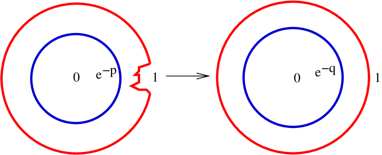
Figure 2: Uniformizing map.

Let $G_{p}$ be the group acting on $\mathbb{C}^{*}$ generated by the two transformations $S_{0}:Z\rightarrow 1/\overline{Z}$ and $S_{p}:Z\rightarrow e^{-2p}/\overline{Z}$. As abstract groups, $G_{p}$ and $G_{q}$ are isomorphic via $S_{0}\leftrightarrow S_{0}$, $S_{p}\leftrightarrow S_{q}$ : we write $T_{p}$ for a generic element in $G_{p}$ and $T_{q}$ for the corresponding element of $G_{q}$. Note that $\mathbb{A}_{q}$ is a fundamental domain for the action of $G_{q}$ on $\mathbb{C}^{*}$. Let $\mathbb{C}^{*}(p,\mathbb{K})\equiv\mathbb{C}^{*}\setminus\cup_{T_{p}\in G_{p}}T_{p}(\overline{\mathbb{K}})$ be the connected open subset of $\mathbb{C}^{*}$ obtained by removal of the $G_{p}$-translates of the closure of $\mathbb{K}$, see Figure(3).

The Schwarz symmetry principle implies that $g$ can be extended to a holomorphic function on $\mathbb{C}^{*}(p,\mathbb{K})$ by $g(T_{p}(Z))=T_{q}(g(Z))$. This extension satisfies

$$g(1/\overline{Z})=1/\overline{g(Z)},\qquad g(e^{-2p}/\overline{Z})=e^{-2q}/\overline{g(Z)},\quad Z\in\mathbb{C}^{*}(p,\mathbb{K}).$$ (9)

The relationship between $p$, $q$ and $\mathbb{K}$ is non trivial.

In the infinitesimal case, when $\mathbb{K}$ is a compact strict subset of the circle $|Z|=1$, we write $g(Z)=Z+\epsilon v(Z)$ for some holomorphic vector field on $\mathbb{C}^{*}(p,\mathbb{K})$ and $q=p-\epsilon s$. Eqs.(9) for $g$ translate into

$$v(1/\overline{Z})=-\overline{v(Z)}/\overline{Z}^{2}\qquad e^{2p}v(e^{-2p}/\overline{Z})=-\overline{v(Z)}/\overline{Z}^{2}+2s/\overline{Z}$$ (10)

for the vector field $v$.

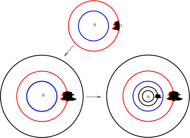
Figure 3: Recursive construction of $\mathbb{C}^{*}(p,\mathbb{K})$ and extension of the holomorphy domain by successive Schwarz symmetries.

To describe the case of an infinitesimal slit emerging from $1$, we impose that $\mathbb{K}=\{1\}$ and $v(Z)\sim-\frac{2}{Z-1}$ for $Z\rightarrow 1$. A lengthy but elementary computation shows that the above system has no solution if $s\neq 1$ and that if $s=1$ the most general solution is an automorphic form :

$$v(Z)/Z=1+i\lambda-2\left(\sum_{m\geq 0}\frac{Z}{Z-e^{2mp}}+\sum_{m<0}\frac{e^{2mp}}{Z-e^{2mp}}\right),$$

where $\lambda$ is an arbitrary real parameter. As usual, $w_{-1}$ is the generator associated to the $\lambda$-ambiguity and imposing left-right symmetry leads to

$$w_{-1}=-iZ\partial_{Z}\qquad w_{-2}^{[p]}=\left(\frac{Z(Z+1)}{2(Z-1)}+\sum_{m>0}\frac{Z^{2}}{Z-e^{2mp}}+\sum_{m<0}\frac{Ze^{2mp}}{Z-e^{2mp}}\right)\partial_{Z}.$$

One can check that $w_{-2}^{[p]}$ vanishes at $Z=-1$, as suggested by symmetry.

Several remarks are in order. The vector field $w_{-1}=-iZ\partial_{Z}$ is the same as for radial SLE. A new feature is the dependence of $w_{-2}$ on the moduli $p$. When $p\rightarrow+\infty$, one recovers radial SLE. As expected, $s$ is not an independent parameter but is determined by $\mathbb{K}$. The value $s=1$ that we found implies that if we iterate infinitesimal slits to make a Loewner evolution, the parameter of the annulus varies linearly : $q=p-t$ with the normalizations we have chosen. This leads to a slight modification of eq.(1) :

$$df_{t}(z)=dt\,\sigma^{[p-t]}(f_{t}(z))+d\xi_{t}\,\rho(f_{t}(z))$$

with $\sigma^{[p]}$ and $\rho$ related to $w_{-1}$ and $w_{-2}$ as in eq.(3). Standard arguments lead to the existence of local (in time and space) solutions of this equation with initial data $f_{0}(z)=z$. Correspondingly, eq.(4) becomes :

$$\gamma_{f_{t}}^{-1}\cdot d\gamma_{f_{t}}=dt\,(-2w_{-2}^{[p-t]}+\frac{\kappa}{2}w_{-1}^{2})-d\xi_{t}\,w_{-1}.$$

The corresponding ordinary differential equation for $g_{t}\equiv e^{\xi_{t}w_{-1}}\cdot f_{t}$ is

$$\frac{dg_{t}(z)}{dt} = g_{t}(z)\frac{1+g_{t}(z)e^{i\xi_{t}}}{1-g_{t}(z)e^{i\xi_{t}}}+2\sum_{m>0}\frac{g_{t}(z)^{2}e^{i\xi_{t}}}{e^{2m(p-t)}-g_{t}(z)e^{i\xi_{t}}}$$

$$\hskip 90.19518pt+2\sum_{m<0}\frac{g_{t}(z)e^{2m(p-t)}}{e^{2m(p-t)}-g_{t}(z)e^{i\xi_{t}}}.$$

This time we have, alas, yet no natural group to interpret $\gamma_{f_{t}}$ or $\gamma_{g_{t}}$, because no point is fixed under the evolution.

At time $t=t_{c}\equiv p$, the evolution terminates because the hull touches the inner boundary of the annulus, and the distribution of the hitting point is one of the first problems that comes to mind. This question is related to the behavior of the solutions of the stochastic differential equation that describes the motion of points on the inner boundary $|Z|=e^{-p+t}$ at time $t$. Setting $f_{t}=e^{\zeta_{t}}$, the stochastic differential equation eq.(1) becomes

$$d\zeta_{t}=id\xi_{t}+dt\left(1-2\sum_{m\geq 0}\frac{e^{\zeta_{t}}}{e^{\zeta_{t}}-e^{2m(p-t)}}-2\sum_{m<0}\frac{e^{2m(p-t)}}{e^{\zeta_{t}}-e^{2m(p-t)}}\right)$$

The motion of points on the outer and inner boundary are different. The motion of points on the outer boundary $|Z|=1$ is obtained by imposing $\zeta_{t}=i\theta_{t}$ with real $\theta_{t}$. This is consistent with the stochastic differential equation and leads to

$$d\theta_{t}=d\xi_{t}+dt\left(\cot\frac{\theta_{t}}{2}+2\sum_{m>0}\frac{\sin\theta_{t}}{\cosh 2m(p-t)-\cos\theta_{t}}\right).$$

The motions of points on the inner boundary $|Z|=e^{t-p}$ is obtained by setting $\zeta_{t}=t-p+i\varphi_{t}$. This is again consistent with the stochastic differential equation and leads to

$$d\varphi_{t}=d\xi_{t}+2dt\sum_{m\geq 0}\frac{\sin\varphi_{t}}{\cosh(2m+1)(p-t)-\cos\varphi_{t}}.$$

The $dt$ coefficient in the equations for $\theta_{t}$ and $\varphi_{t}$ becomes singular when $t\rightarrow t_{c}=p$. These motions are closely related to the elliptic Calogero Hamiltonian, but not identical because of the explicit time dependence.

To conclude this discussion of SLE avatars, let us mention that from the original point of view of Loewner deterministic evolutions in the annular case, it may be more natural to work with a Loewner uniformizing map that fixes a point on the outer circle of the annulus, say $1$, to describe a growing hull starting from the inner circle. The corresponding vector field is of course again given by some automorphic form, but slightly different from our $w_{-2}$. However, in that case there is no automorphism left, so our formalism based on symmetries gives no clue to define a Brownian source in a natural way. There is probably a nice SLE in that situation too, so that a more unifying idea is needed to get a hand on general SLEs.

3 CFTs of chordal SLEs.

We now describe the relation between SLE and conformal field theory (CFT) which we developed in ref.[7]. Another approach has been presented in ref.[10].

Recall that $f_{t}(z)\equiv g_{t}(z)-\xi_{t}$ satisfies the stochastic differential equation

$$df_{t}=\frac{2dt}{f_{t}}-d\xi_{t}.$$

According to section (2.2), to $f_{t}$ we can associate $\gamma_{f_{t}}\in N_{-}$, with $N_{-}$ the group of germs of holomorphic functions at $\infty$ of the form $z+\sum_{m\leq-1}f_{m}z^{m+1}$. By Itô’s formula, it satisfies:

$$\gamma_{f_{t}}^{-1}\cdot d\gamma_{f_{t}}=dt(\frac{2}{z}\partial_{z}+\frac{\kappa}{2}\partial_{z}^{2})-d\xi_{t}\partial_{z}.$$ (11)

The operators $\ell_{n}=-z^{n+1}\partial_{z}$ are represented in conformal field theories by operators $L_{n}$ which satisfy the Virasoro algebra $\mathfrak{vir}$, see eq.(5). We need to recall a few basic facts concerning the Virasoro algebra and its highest weight representations. These representations possess a highest weight vector $|h\rangle$ are such that $L_{n}|h\rangle=0$ for $n>0$ and $L_{0}|h\rangle=h|h\rangle$. The parameter $h$ is called the conformal dimension of the representation. Define

$$h_{r;s}={[(r\kappa-4s)^{2}-(\kappa-4)^{2}]}/{16\kappa}$$

for

$$c=1-6{(\kappa-4)^{2}}/{4\kappa}.$$

Values of $h_{r;s}$, $r,s=1,2,\cdots$ label degenerate highest weight representations of the Virasoro algebra, with a singular vector at level $rs$. Many interesting conformal weights that appear in CFTs of SLEs are related to simple integral or half integral values of $r$ and $s$.

The representations of $\mathfrak{vir}$ are not automatically representations of $N_{-}$, one of the reasons being that the Lie algebra of $N_{-}$ contains infinite linear combinations of the $\ell_{n}$’s. However, as we shall explain in section 5, highest weight representations of $\mathfrak{vir}$ can be extended in such a way that $N_{-}$ get embedded in a appropriate completion $\overline{\mathcal{U}(\mathfrak{n}_{-})}$ of the enveloping algebra of some sub-algebra $\mathfrak{n}_{-}$ of $\mathfrak{vir}$. This will allows us to associate to any $\gamma_{f}\in N_{-}$ an operator $G_{f}$ acting on appropriate representations of $\mathfrak{vir}$ and satisfying $G_{g\circ f}=G_{f}G_{g}$. Implementing this construction for $f_{t}$ yields random operators $G_{t}\equiv G_{f_{t}}\in\overline{\mathcal{U}(\mathfrak{n}_{-})}$ which satisfy the stochastic Itô equation [7]:

$$G_{t}^{-1}dG_{t}=dt(-2L_{-2}+\frac{\kappa}{2}L_{-1}^{2})+d\xi_{t}L_{-1}.$$ (12)

Compare with eq.(11). This may be viewed as defining a Markov process in $\overline{\mathcal{U}(\mathfrak{n}_{-})}$.

Since $G_{t}$ turns out to be the operator intertwining the conformal field theories in $\mathbb{H}$ and in the random domain $\mathbb{H}_{t}$, the basic observation which allows us to couple CFTs to SLEs is the following [7]:

Let $|\omega\rangle\equiv|h_{1;2}\rangle$ be the highest weight vector in the irreducible highest weight representation of $\mathfrak{vir}$ of central charge $c_{\kappa}=\frac{(6-\kappa)(3\kappa-8)}{2\kappa}$ and conformal weight $h_{\kappa}\equiv h_{1;2}=\frac{6-\kappa}{2\kappa}$.

Then $G_{t}|\omega\rangle$ is a local martingale.

Assuming appropriate boundedness conditions on $\langle v|$, the scalar $\langle v|G_{t}|\omega\rangle$ is a martingale so that ${\bf E}[\langle v|G_{t}|\omega\rangle|\{{G_{u}}\}_{u\leq s}]$ is time independent for $t\geq s$ and:

$${\bf E}[\,\langle v|G_{t}|\omega\rangle\,|\{G_{u}\}_{u\leq s}]=\langle v|G_{s}|\omega\rangle$$ (13)

This result is a direct consequence of eq.(12) and the null vector relation $(-2L_{-2}+\frac{\kappa}{2}L_{-1}^{2})|\omega\rangle=0$ so that $dG_{t}|\omega\rangle=G_{t}L_{-1}|\omega\rangle d\xi_{t}$.

This result has the following consequences. Consider CFT correlation functions in $\mathbb{H}_{t}$. They can be computed by looking at the same theory in $\mathbb{H}$ modulo the insertion of an operator representing the deformation from $\mathbb{H}$ to $\mathbb{H}_{t}$, see the next section. This operator is $G_{t}$. Suppose that the central charge is $c_{\kappa}$ and the boundary conditions are such that there is a boundary changing primary operator of weight $h_{1;2}$ inserted at the tip of $\mathbb{K}_{t}$. Then in average the correlation functions of the conformal field theory in the fluctuating geometry $\mathbb{H}_{t}$ are time independent and equal to their value at $t=0$.

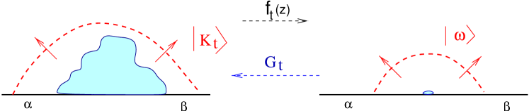
Figure 4: A representation of the boundary hull state and of the map intertwining different formulations of the CFT.

The state $G_{t}|\omega\rangle$ may be interpreted as follows. Imagine defining the conformal field theory in $\mathbb{H}_{t}$ via a radial quantization, so that the conformal Hilbert spaces are defined over curves topologically equivalent to half circles around the origin. Then, the SLE hulls manifest themselves as disturbances localized around the origin, and as such they generate states in the conformal Hilbert spaces. Since $G_{t}$ intertwines the CFT in $\mathbb{H}$ and in $\mathbb{H}_{t}$, these states are $G_{t}|\omega\rangle$ with $|\omega\rangle$ keeping track of the boundary conditions. See Figure (4).

4 CFTs of other SLEs.

The degenerate representation with highest weight state $|\omega\rangle$ plays a fundamental role in radial, dipolar and annular SLE as well, and we would like to see this explicitly in this short section.

In all cases we can choose the geometry in such a way that the real axis is a boundary globally fixed by the SLE evolution and that $w_{-1}$ and $w_{-2}$ where meromorphic in a neighborhood of the origin, with computable small $z$ expansion. The embedding $\ell_{n}\rightarrow L_{n}$ allows to turn $w_{-1}$ and $w_{-2}$ into operators $W_{-1}$ and $W_{-2}$. In all cases, $|\omega\rangle$ turns out to be an eigenvector of the diffusion operator $\mathcal{A}=-2W_{-2}+\frac{\kappa}{2}W_{-1}^{2}$. Let us see this explicitly.

Radial SLE : We have seen that $w_{-1}=\ell_{-1}+\ell_{1}$ and $w_{-2}=\ell_{-2}+\ell_{0}$, so that

$$W_{-1}=L_{-1}+L_{1}\qquad W_{-2}=L_{-2}+L_{0}.$$

A simple rearrangement leads to

$$-2W_{-2}+\frac{\kappa}{2}W_{-1}^{2}=\left(-2L_{-2}+\frac{\kappa}{2}L_{-1}^{2}\right)+(\kappa-2)L_{0}+\kappa L_{-1}L_{1}+\frac{\kappa}{2}L_{1}^{2},$$

Finally

$$\mathcal{A}|\omega\rangle=\frac{(\kappa-2)(6-\kappa)}{2\kappa}|\omega\rangle=8h_{0;1/2}|\omega\rangle.$$

If $G_{t}$ represents the action of $\gamma_{f_{t}}$ in the radial case we find that

$$M_{t}\equiv e^{-8h_{0;1/2}t}G_{t}|\omega\rangle$$

is a local martingale. The prefactor $e^{-8h_{0;1/2}t}$ accounts for the insertion of a bulk conformal field of scaling dimension $2h_{0;1/2}$ localized at the fixed point, see ref.[18] for further details.

Dipolar SLE : We have seen that $w_{-1}=\ell_{-1}-\ell_{1}$ and $w_{-2}=\ell_{-2}-\ell_{0}$, so that

$$W_{-1}=L_{-1}-L_{1}\qquad W_{-2}=L_{-2}-L_{0}.$$

and by the same rearrangement

$$\mathcal{A}|\omega\rangle=-\frac{(\kappa-2)(6-\kappa)}{2\kappa}|\omega\rangle=-8h_{0;1/2}|\omega\rangle.$$

If $G_{t}$ represents the action of $\gamma_{f_{t}}$ in the dipolar case (we have given two natural candidates) we find that

$$M_{t}\equiv e^{8h_{0;1/2}t}G_{t}|\omega\rangle$$

is a local martingale. The prefactor $e^{+8h_{0;1/2}t}$ accounts for the insertion of two boundary conformal fields, each of dimension $h_{0;1/2}$, localized at the two fixed points which are the end points of the forbidden zone.

Annular SLE : To see the relation with the Virasoro algebra, we go to a more convenient geometry. The change of variable $z=i\frac{1-Z}{1+Z}$ maps the annulus to the complement of a disk in the upper-half plane $\mathbb{H}$. In the new variable one obtains $w_{-1}=-\frac{1}{2}(1+z^{2})\partial_{z}$, and

$$w_{-2}^{[p]}=-\frac{1}{4}(1+z^{2})\left(\frac{1}{z}+2z\sum_{m>0}\frac{1}{z^{2}\cosh^{2}mp+\sinh^{2}mp}\right)\partial_{z}.$$

The time change to recover the standard normalization is not so convenient here because of the explicit dependence on the modulus, hence on time. Expansion in powers of $z$ reveals that $w_{-1}=\frac{1}{2}(\ell_{-1}+\ell_{1})$ and

$$w_{-2}^{[p]}=\sum_{n\geq-1}a_{n}\ell_{2n}=\frac{1}{4}\ell_{-2}+\frac{1}{4}\left(1+2\sum_{m>0}\frac{1}{\sinh^{2}mp}\right)\ell_{0}+\cdots,$$

with

$$a_{n}=\frac{(-)^{n}}{2}\sum_{m>0}\frac{\cosh^{2n-2}mp}{\sinh^{2n+2}mp},\;n\geq 1.$$

Hence

$$W_{-1}=\frac{1}{2}(L_{-1}+L_{1})\qquad W_{-2}^{[p]}=\frac{1}{4}L_{-2}+\frac{1}{4}\left(1+2\sum_{m>0}\frac{1}{\sinh^{2}mp}\right)L_{0}+\cdots$$

where the missing terms annihilate $|\omega\rangle$. So :

$$\mathcal{A}^{[p]}|\omega\rangle=\left(2h_{0;1/2}-h_{1;2}\sum_{m>0}\frac{1}{\sinh^{2}mp}\right)|\omega\rangle.$$

The new feature is that the eigenvalue is time dependent : it involves the second Eisenstein series in elliptic function theory.

For the annular case, we have not constructed explicitly the spaces $O$ and $N$ so the existence of $\gamma_{f_{t}}$ remains hypothetical. From a physical viewpoint however, the existence of the action of $G_{t}$ in conformal field theory makes little doubt, and

$$M_{t}\equiv\frac{e^{-2h_{0;1/2}t}}{\prod_{m>0}\left(1-e^{2m(t-p)}\right)^{2h_{1;2}}}\;G_{t}|\omega\rangle$$

should be a local martingale. For large $p$, we retrieve the radial formula. The prefactor is closely related to the classical partition function, or equivalently to the Dedekind $\eta$ function. Its modular properties allow to rewrite

$$M_{t}=e^{-2h_{0;1/2}t}\left(\frac{(p-t)^{\frac{1}{2}}e^{-\frac{p-t}{12}+\frac{\pi^{2}}{12(p-t)}}}{\pi^{\frac{1}{2}}\prod_{m>0}\left(1-e^{\frac{2m\pi^{2}}{t-p}}\right)}\right)^{2h_{1;2}}G_{t}|\omega\rangle,$$

which gives the limiting behavior when $t\rightarrow t_{c}=p$.

5 Conformal transformations in CFT and applications.

Recall that we are using boundary CFT on $\mathbb{H}_{t}$, the complement of the SLE hulls, to probe these hulls. We thus need to know how to implement algebraically conformal maps in CFT.

The basic principles of conformal field theory state that correlation functions in a domain $\mathbb{U}$ are known once they are known in a domain $\mathbb{U}_{0}$ and an explicit conformal map $f$ from $\mathbb{U}$ to $\mathbb{U}_{0}$ preserving boundary conditions is given. Primary fields have a very simple behavior under conformal transformations: for a bulk primary field $\Phi$ of weight $(h,\overline{h})$, $\Phi(z,\overline{z})dz^{h}d\overline{z}^{\overline{h}}$ is invariant, and for a boundary conformal field $\Psi$ of weight $\delta$, $\Psi(x)|dx|^{\delta}$ is invariant. Their statistical correlations in $\mathbb{U}$ and $\mathbb{U}_{0}$ are related by

$$\langle\cdots\Phi(z,\overline{z})\cdots\Psi(x)\cdots\rangle_{\mathbb{U}}$$

$$\hskip-42.67912pt=\langle\cdots\Phi(f(z),\overline{f(z)})f^{\prime}(z)^{h}\overline{f^{\prime}(z)}^{\overline{h}}\cdots\Psi(f(x))|f^{\prime}(x)|^{\delta}\cdots\rangle_{\mathbb{U}_{0}}.$$ (14)

Infinitesimal deformations of the underlying geometry are implemented in local field theories by insertions of the stress-tensor. In conformal field theories, the stress-tensor is traceless so that it has only two independent components, one of which, $T(z)$, is holomorphic (except for possible singularities when its argument approaches the arguments of other inserted operators). The field $T(z)$ itself is not a primary field but a projective connection,

$$\langle\cdots T(z)\cdots\rangle_{\mathbb{U}}=\langle\cdots T(f(z))f^{\prime}(z)^{2}+\frac{c}{12}\mathrm{S}f(z)\cdots\rangle_{\mathbb{U}_{0}},$$

with $c$ the CFT central charge and $\mathrm{S}f(z)=\left(\frac{f^{\prime\prime}(z)}{f^{\prime}(z)}\right)^{\prime}-\frac{1}{2}\left(\frac{f^{\prime\prime}(z)}{f^{\prime}(z)}\right)^{2}$ the Schwarzian derivative of $f$ at $z$.

This applies to infinitesimal deformations of the upper half plane. Consider an infinitesimal hull $\mathbb{K}_{\epsilon;\mu}$, whose boundary is the curve $x\to\epsilon\,\pi\mu(x)$, $x$ real and $\epsilon\ll 1$, so that $\mathbb{K}_{\epsilon;\mu}=\{z=x+iy\in\mathbb{H},\ 0<y<\epsilon\,\pi\mu(x)\}$. Assume for simplicity that $\mathbb{K}_{\epsilon;\mu}$ is bounded away from $0$ and $\infty$. Let $\mathbb{H}_{\epsilon;\mu}\equiv\mathbb{H}\setminus\mathbb{K}_{\epsilon;\mu}$. To first order in $\epsilon$, the uniformizing map onto $\mathbb{H}$ is

$$z+\epsilon\,\int_{\mathbb{R}}\frac{\mu(y)dy}{z-y}+o(\epsilon).$$

To first order in $\epsilon$ again, correlation functions in $\mathbb{H}_{\epsilon;\mu}$ are related to those in $\mathbb{H}$ by insertion of $T$:

$$\frac{d}{d\epsilon}\langle\left(\cdots\Phi(z,\overline{z})\cdots\Psi(x)\cdots\right)\rangle_{\mathbb{H}_{\epsilon;\mu}}\Big{|}_{\epsilon=0^{+}}$$

$$\hskip-42.67912pt=-\int_{\mathbb{R}}dy\mu(y)\,\langle T(y)\left(\cdots\Phi(z,\overline{z})\cdots\Psi(x)\cdots\right)\rangle_{\mathbb{H}}$$ (15)

With the basic CFT relation [1] between the stress tensor and the Virasoro generators, $T(z)=\sum_{n}L_{n}z^{n-2}$, this indicates that infinitesimal deformations of the domains are described by insertions of elements of the Virasoro algebra.

Finite conformal transformations are implemented in conformal field theories by insertion of operators, representing some appropriate exponentiation of insertions of the stress tensor. Let $\mathbb{U}$ be conformally equivalent to the upper half plane $\mathbb{H}$ and $f$ the corresponding uniformizing map. Then, following [9], the finite conformal deformations that leads from the conformal field theory on $\mathbb{U}$ to that on $\mathbb{H}$ can be represented by an operator $G_{f}$:

$$\langle\cdots\Phi(z,\overline{z})\cdots\Psi(x)\cdots\rangle_{\mathbb{U}}=\langle G_{f}^{-1}\left(\cdots{\Phi}(z,\overline{z})\cdots{\Psi}(x)\cdots\right)G_{f}\rangle_{\mathbb{H}}.$$ (16)

This relates correlation functions in $\mathbb{U}$ to correlation functions in $\mathbb{H}$ where the field arguments are taken at the same point but conjugated by $G_{f}$. Radial quantization is implicitly assumed in eq.(16). Compare with eq.(14).

The following is a summary, extracting the main steps, of a construction of $G_{f}$ described in details in [9]. To be more precise, we need to distinguish cases depending whether $f$ fixes the origin or the point at infinity. We also need a few simple definitions. We let $\mathfrak{vir}$ be the Virasoro algebra generated by the $L_{n}$ and $c$, and $\mathfrak{n}_{-}$ (resp. $\mathfrak{n}_{+}$) be the nilpotent Lie sub-algebra of $\mathfrak{vir}$ generated by the $L_{n}$’s, $n<0$ (resp. $n>0$), and by $\mathfrak{b}_{-}$ (resp. $\mathfrak{b}_{+}$) the Borel Lie sub-algebra of $\mathfrak{vir}$ generated by the $L_{n}$’s, $n\leq 0$ (resp. $n\geq 0$) and $c$. We denote by $\overline{\mathcal{U}(\mathfrak{n}_{-})}$ (resp. $\overline{\mathcal{U}(\mathfrak{n}_{+})}$) appropriate completion of the enveloping algebra of $\mathfrak{n}_{-}$ (resp. $\mathfrak{n}_{+}$). We shall only consider highest weight vector representations of the Virasoro algebra.

5.1 Finite deformations fixing $0$.

Let $N_{+}$ be the space of power series of the form $z+\sum_{m\geq 1}f_{m}z^{m+1}$ which have a non vanishing radius of convergence. With words, $N_{+}$ is the set of germs of holomorphic functions at the origin fixing the origin and whose derivative at the origin is $1$. In applications to the chordal SLE, we shall only need the case when the coefficients are real. But it is useful to consider the $f_{m}$’s as independent commuting indeterminates.

$N_{+}$ is a group for composition. Our aim is to construct a group (anti)-isomorphism from $N_{+}$ with composition onto a subset $\mathcal{N}_{+}\subset\overline{\mathcal{U}(\mathfrak{n}_{+})}$ with the associative algebra product.

We let $N_{+}$ act on $O_{0}$, the space of germs of holomorphic functions at the origin, by $\gamma_{f}\cdot F\equiv F\circ f$ for $f\in N_{+}$ and $F\in O_{0}$. This representation is faithful and $\gamma_{g\circ f}=\gamma_{f}\gamma_{g}$. We need to know how $\gamma_{f}$ varies when $f$ varies as $f\to f+\varepsilon v(f)$ for small $\varepsilon$ and an arbitrary vector field $v$. Taking $g=z+\varepsilon v(z)$ in the group law leads to $\gamma_{f+\varepsilon v(f)}F=\gamma_{f}\cdot F+\varepsilon\gamma_{f}\cdot(v\cdot F)+o(\varepsilon)$, where $v\cdot F(z)\equiv v(z)F^{\prime}(z)$ is the standard action of vector fields on functions. Using Lagrange inversion formula to determine the vector field $v$ corresponding to the variation of the indeterminate $f_{m}$ yields:

$$\gamma_{f}^{-1}\,\frac{\partial\gamma_{f}}{\partial f_{m}}=\sum_{n\geq m}\left(\oint_{0}\frac{dw}{2i\pi}w^{m+1}\frac{f^{\prime}(w)}{f(w)^{n+2}}\right)\,z^{n+1}\partial_{z}.$$

This system of first order partial differential equations makes sense in $\overline{\mathcal{U}(\mathfrak{n}_{+})}$ if we replace $\ell_{n}=-z^{n+1}\partial_{z}$ by $L_{n}$. So, we define a connection $A_{m}$ in $\overline{\mathcal{U}(\mathfrak{n}_{+})}$ by

$$A_{m}(f)\equiv\sum_{n\geq m}L_{n}\,\left(\oint_{0}\frac{dw}{2i\pi}w^{m+1}\frac{f^{\prime}(w)}{f(w)^{n+2}}\right)$$

which by construction satisfies the zero curvature condition, $\frac{\partial A_{l}}{\partial f_{k}}-\frac{\partial A_{k}}{\partial f_{l}}=[A_{k},A_{l}].$

We may thus construct an element $G_{f}\in\mathcal{N}_{+}\subset\overline{\mathcal{U}(\mathfrak{n}_{+})}$ for each $f\in N_{+}$ by solving the system

$$\frac{\partial G_{f}}{\partial f_{m}}=-G_{f}A_{m}(f),\qquad m\geq 1.$$ (17)

This system is guaranteed to be compatible, because $N_{+}$ is convex and the representation of $N_{+}$ on $O_{0}$ is well defined for finite deformations $f$, faithful and solves the analogous system. The existence and uniqueness of $G_{f}$, with the initial condition $G_{f=z}=1$, is clear and the group (anti)-homomorphism property, $G_{f}G_{g}=G_{g\circ f}$, is true because it is true infinitesimally and $N_{+}$ is convex. To lowest orders: $G_{f}=1-f_{1}L_{1}+\frac{f_{1}^{2}}{2}(L_{1}^{2}+2L_{2})-f_{2}L_{2}+\cdots.$

The element $G_{f}$, acting on a highest weight representation of the Virasoro algebra, is the operator which implements the conformal map $f$ in conformal field theory. It acts on the stress tensor by conjugation as:

$$G_{f}^{-1}T(z)G_{f}=T(f(z))f^{\prime}(z)^{2}+\frac{c}{12}Sf(z),$$ (18)

a formula which makes sense as long as $z$ is in the disk of convergence of $f^{\prime}(z)$ and $Sf(z)$, but which can be extended by analytic continuation if $f(z)$ allows it. A similar formula would hold if we would have considered the action of $G_{f}$ on local fields. In particular, by eq.(18), $G_{f}$ induces an automorphism of the Virasoro algebra by $L_{m}\to L_{m}(f)\equiv G_{f}^{-1}L_{m}G_{f}$ with $G_{f}^{-1}T(z)G_{f}=\sum_{m}L_{m}(f)z^{-m-2}$:

$$G_{f}^{-1}L_{m}G_{f}=\frac{c}{12}\,\left(\oint_{0}\frac{dw}{2i\pi}w^{m+1}Sf(w)\right)+\sum_{n\geq m}L_{n}\,\left(\oint_{0}\frac{dw}{2i\pi}w^{m+1}\frac{f^{\prime}(w)^{2}}{f(w)^{n+2}}\right).$$

Eq.(17), which specifies the variations of $G_{f}$, can be rewritten in a maybe more familiar way involving the stress tensor. Namely, if $f$ is changed to $f+\delta f$ with $\delta f=\varepsilon v(f)$, then:

$$\delta G_{f}=-\varepsilon\,G_{f}\,\oint_{0}\frac{dz}{2i\pi}\,T(z)\,v(z).$$

If $v$ is not just a formal power series at the origin, but a convergent one in a neighborhood of the origin, we can freely deform contours in this formula, thus making contact with the infinitesimal deformations considered in eq.(15).

5.2 Finite deformations fixing $\infty$.

All the previous considerations could be extended to the case in which the holomorphic functions fix $\infty$ instead of $0$. Let $N_{-}$ be the space of power series of the form $z+\sum_{m\leq-1}f_{m}z^{m+1}$ which have a non vanishing radius of convergence. We let it act on $O_{\infty}$, the space of germs of holomorphic functions at infinity, by $\gamma_{f}\cdot F\equiv F\circ f$. The adaptation of the previous computations shows that $\gamma_{f}^{-1}\frac{\partial\gamma_{f}}{\partial f_{m}}=\sum_{n\leq m}\left(\oint_{\infty}\frac{dw}{2i\pi}w^{m+1}\frac{f^{\prime}(w)}{f(w)^{n+2}}\right)z^{n+1}\partial_{z}.$ We transfer this relation to $\overline{\mathcal{U}(\mathfrak{n}_{-})}$ to define an (anti)-isomorphism from $N_{-}$ to $\mathcal{N}_{-}\subset\overline{\mathcal{U}(\mathfrak{n}_{-})}$ mapping $f$ to $G_{f}$ such that

$$\frac{\partial G_{f}}{\partial f_{m}}=-G_{f}\sum_{n\leq m}L_{n}\,\left(\oint_{\infty}\frac{dw}{2i\pi}w^{m+1}\frac{f^{\prime}(w)}{f(w)^{n+2}}\right),\qquad m\leq-1.$$

5.3 Dilatations and translations.

We have been dealing with deformations around $0$ and $\infty$ that did not involve dilatation at the fixed point: $f^{\prime}(0)$ or $f^{\prime}(\infty)$ was unity. To gain some flexibility we may also authorize dilatations, say at the origin. The operator associated to a pure dilatation $z\to\lambda z$ is $\lambda^{-L_{0}}$. One can view a general $f$ fixing $0$ as the composition $f(z)=f^{\prime}(0)(z+\sum_{m}f_{m}z^{m+1})$ of a deformation at $0$ with derivative $1$ at $0$ followed by a dilatation, so that $G_{f}=G_{f/f^{\prime}(0)}\,f^{\prime}(0)^{-L_{0}}.$

We may also implement translations. Suppose that $f(z)=f^{\prime}(0)(z+\sum_{m}f_{m}z^{m+1})$ is a generic invertible germ of holomorphic function fixing the origin. If $a$ is in the interior of the disk of convergence of the power series expansion of $f$ and $f^{\prime}(a)\neq 0$, we may define a new germ $f_{a}(z)\equiv f(a+z)-f(a)$ with the same properties. The operators $G_{f}$ and $G_{f_{a}}$ implementing $f$ and $f_{a}$ are then related by $G_{f_{a}}=e^{-aL_{-1}}\,G_{f}\,e^{f(a)L_{-1}}.$

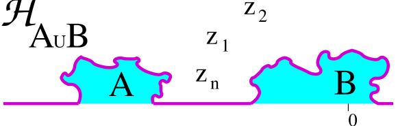
Figure 5: A typical two hull geometry.

5.4 Deformations around $0$ and $\infty$ and ‘Virasoro Wick theorem’.

Consider now a domain $\mathbb{H}_{A\cup B}$ of the type represented on Figure(5) which is the complement of two disjoint hulls, the first one, say $A$, located around infinity but away from the origin, and the second one, say B, located around the origin and away from infinity. The uniformizing map $f_{A\cup B}$ of $\mathbb{H}_{A\cup B}$ onto $\mathbb{H}$ then does not exist at $0$ or at $\infty$.

However, in this situation, we may obtain the map $f_{A\cup B}$ by first removing $B$ by $f_{B}$, which is regular around $\infty$ and such that $f_{B}(z)=z+O(1)$ at infinity, and then $\widetilde{A}\equiv f_{B}(A)$ by $f_{\widetilde{A}}$ which is regular around $0$ and fixes $0$ ($f_{\widetilde{A}}^{\prime}(0)\neq 1$ is allowed). Of course, the roles of $A$ and $B$ could be interchanged, and we could first remove $A$ by $f_{A}$ which is regular around $0$ and fixes $0$ and then $\widetilde{B}\equiv f_{A}(B)$ by $f_{\widetilde{B}}$ which is regular around $\infty$ and such that $f_{\widetilde{B}}(z)=z+O(1)$.

Suppose that $f_{A}$ and $f_{B}$ are given. There is some freedom in the choice of $f_{\widetilde{A}}$ and $f_{\widetilde{B}}$ : namely we can replace $f_{\widetilde{A}}$ by $h_{0}\circ f_{\widetilde{A}}$ where $h_{0}\in PSL_{2}(\mathbb{R})$ fixing $0$, and $f_{\widetilde{B}}$ by $h_{\infty}\circ f_{\widetilde{B}}$ where $h_{\infty}\in PSL_{2}(\mathbb{R})$ such that $h_{\infty}(z)=z+O(1)$ at infinity, i.e. a translation. A simple computation shows that generically there is a unique choice of $f_{\widetilde{A}}$ and $f_{\widetilde{B}}$ such that $f_{\widetilde{B}}\circ f_{A}=f_{\widetilde{A}}\circ f_{B}$ and both equal to $f_{A\cup B}$. This commutative diagram was introduced in [5].

For sufficiently disjoint hulls $A$ and $B$, as in Figure(5), there exists an open set such that for $z$ in this set, both products $G^{-1}_{f_{\widetilde{A}}}\left(G^{-1}_{f_{B}}T(z)G_{f_{B}}\right)G_{f_{\widetilde{A}}}$ and $G^{-1}_{f_{\widetilde{B}}}\left(G^{-1}_{f_{A}}T(z)G_{f_{A}}\right)G_{f_{\widetilde{B}}}$ are well defined, given by absolutely convergent series, and are both equal to $T(f_{A\cup B}(z))f^{\prime}_{A\cup B}(z)^{2}+\frac{c}{12}Sf_{A\cup B}(z)$. As the modes $L_{n}$ of $~{}T(z)$ generate all states in a highest weight representation, the operators $G_{f_{B}}G_{f_{\widetilde{A}}}$ and $G_{f_{A}}G_{f_{\widetilde{B}}}$ have to be proportional: they differ at most by a factor involving the central charge $c$. We write $G_{f_{B}}G_{f_{\widetilde{A}}}=Z(A,B)\;G_{f_{A}}G_{f_{\widetilde{B}}},$ or [9]

$$G_{f_{A}}^{-1}\,G_{f_{B}}=Z(A,B)\,G_{f_{\widetilde{B}}}\,G_{f_{\widetilde{A}}}^{-1}.$$ (19)

Formula (19) plays for the Virasoro algebra the role that Wick’s theorem plays for collections of harmonic oscillators. Since $G_{f_{A}}$ and $G_{f_{\widetilde{A}}}$ belong to $\mathcal{N}_{+}$ while $G_{f_{B}}$ and $G_{f_{\widetilde{B}}}$ to $\mathcal{N}_{-}$, eq.(19) may also be viewed as defining a product between elements in $\mathcal{N}_{+}$ and $\mathcal{N}_{-}$. Note that $G_{f_{\widetilde{B}}}\,G_{f_{\widetilde{A}}}^{-1}$ is clearly well defined in highest weight vector representations of $\mathfrak{vir}$.

As implicit in the notation, $Z(A,B)$ depends only on $A$ and $B$: a simple computation shows that it is invariant if $f_{A}$ is replaced by $h_{0}\circ f_{A}$ and $f_{B}$ by $h_{\infty}\circ f_{B}$. It may be evaluated as follows. Let $A_{s}$ and $B_{t}$ be two families of hulls that interpolate between the trivial hull and $A$ or $B$ respectively and $f_{A_{s}}$ and $f_{B_{t}}$ be their uniformizing map. We arrange that $f_{A_{s}}$ and $f_{B_{t}}$ satisfy the genericity condition, so that unique $f_{A_{s,t}}$ and $f_{B_{t,s}}$ exist, which satisfy $f_{B_{t,s}}\circ f_{A_{s}}=f_{A_{s,t}}\circ f_{B_{t}}$. Define vector fields by $v_{A_{s}}$ and $v_{B_{t}}$ by $\frac{\partial f_{A_{s}}}{\partial s}=v_{A_{s}}(f_{A_{s}})$ and $\frac{\partial f_{B_{t}}}{\partial t}=v_{B_{t}}(f_{B_{t}})$. Then [9]:

$$\log Z(A_{\sigma},B_{\tau}) = \frac{c}{12}\int_{0}^{\sigma}ds\oint\frac{dw}{2i\pi}\;v_{A_{s}}(w)Sf_{B_{\tau,s}}(w)$$ (20)

$$= -\frac{c}{12}\int_{0}^{\tau}dt\oint\frac{dz}{2i\pi}\;v_{B_{t}}(z)Sf_{A_{\sigma,t}}(z).$$

$Z(A,B)$ may physically be interpreted as the interacting part of the CFT partition function in $\mathbb{H}\setminus(A\cup B)$.

6 Deformations and Virasoro representations.

The above formula may be used to define generalized coherent state representations of $\mathfrak{vir}$. The key point is to interpret the ‘Virasoro Wick theorem’, eq.(19), as defining an action of $\mathfrak{vir}$ on $\mathcal{N}_{-}$. This is a reformulation of a construction à la Borel-Weil presented in ref.[8].

6.1 Representations around infinity.

Consider first the action of infinitesimal conformal transformations on $N_{-}$, i.e. on functions $f(z)=z+\sum_{m\leq-1}f_{m}z^{m+1}\in N_{-}$. The generator $\ell_{-n}=-z^{1-n}\partial_{z}$, $n>0$ acts on $N_{-}$ by $\widetilde{\delta}_{n}f(z)=-z^{1-n}\,f^{\prime}(z)$. If $n\leq 0$, this infinitesimal variation does not preserve the required behavior of $f$ at infinity and $z^{1-n}\,f^{\prime}(z)$ does not belong to $N_{-}$ for $n\leq 0$. We may however restore this behavior by using the commutative diagram $\widetilde{\phi}\circ f=\widetilde{f}\circ\phi$ with $\phi(z)=z+\varepsilon z^{1-n}$. Then $\widetilde{\phi}(z)=z+\varepsilon\widetilde{y}_{n}(z)$, with $\widetilde{y}_{n}$ polynomial in $z$ of degree $1-n$, and $\widetilde{f}=f+\varepsilon\widetilde{\delta}_{n}f$ belongs to $N_{-}$ with

$$\widetilde{\delta}_{n}f(z)=-z^{1-n}\,f^{\prime}(z)+\widetilde{y}_{n}(f(z))$$ (21)

The polynomial $\widetilde{y}_{n}$ is uniquely fixed by demanding that $\widetilde{\delta}_{n}f(z)=o(z)$ at infinity. Namely, $\widetilde{y}_{n}(w)=\sum_{k}y_{k}w^{k+1}$ with $y_{k}=\oint_{\infty}\frac{dz}{2i\pi}z^{1-n}f^{\prime}(z)^{2}/f(z)^{k+2}$.

Eqs.(21) now define an action of the Virasoro algebra, without central extension, on $N_{-}$. They have a simple interpretation: they are infinitesimal conformal transformations in the source space generated by $\ell_{-n}=-z^{1-n}\partial_{z}$ preserving the normalization at infinity.

To get an action of the Virasoro algebra with central extension, we have to slightly generalize this construction using the ‘Virasoro Wick theorem’. Consider a Verma module $V(c,h)$ and take $x\neq 0$ its highest weight vector. Let $f=z+\sum_{m\leq-1}f_{m}z^{m+1}\in N_{-}$ and $G_{f}$ be the corresponding element in $\mathcal{N}_{-}$. The space $\{P_{y}[f]\equiv\left<y,G_{f}x\right>,y\in V(c,h)^{*}\}$, or $\{Q_{y}[f]\equiv\langle y,G_{f}^{-1}x\rangle,y\in V(c,h)^{*}\}$, is the space of all polynomials in the independent variables $f_{-1},f_{-2},\cdots$. So we have two linear isomorphisms from $V(c,h)^{*}$ to $\mathbb{C}[f_{-1},f_{-2},\cdots]$ and we can use them to transport the action of $\mathfrak{vir}$. We denote by $\mathcal{R}_{n}$ and $\mathcal{S}_{n}$ the differential operators such that

$$\left<L_{n}y,G_{f}x\right>=\mathcal{R}_{n}\left<y,G_{f}x\right>\quad,\quad\langle L_{n}y,G_{f}^{-1}x\rangle=\mathcal{S}_{n}\langle y,G_{f}^{-1}x\rangle$$

for $y\in V^{*}(c,h)$. By construction the operators $\mathcal{R}_{n}$ and $\mathcal{S}_{n}$ are first order differential operators satisfying the Virasoro algebra with non vanishing central charge,

$$[\mathcal{R}_{n},\mathcal{R}_{m}]=(n-m)\mathcal{R}_{n+m}+\frac{c}{12}n(n^{2}-1)\delta_{n;-m},$$

such that $\mathcal{R}_{n}\cdot 1=0$ for $n>0$ and $\mathcal{R}_{0}\cdot 1=h$. Similar results hold for the $\mathcal{S}_{n}$’s. Explicit expressions of these differential operators may be found in ref.[8, 9].

To be a bit more precise, let us consider $P_{y}[f]=\left<y,G_{f}x\right>$ and $P_{L_{n}y}[f]=\mathcal{R}_{n}P_{y}[f]$. We have $\left<L_{n}y,G_{f}x\right>=\left<y,L_{-n}G_{f}x\right>$. If $n>0$, $L_{-n}\in\mathfrak{n}_{-}$, and, by the group law, the product $L_{-n}G_{f}$ corresponds to the infinitesimal variation of $\widetilde{\delta}_{n}f(z)$ generated by $\ell_{-n}=-z^{1-n}\partial_{z}$. If $n\leq 0$, $L_{-n}\in\mathfrak{b}_{+}$ so that we need to re-order the product $L_{-n}G_{f}$ in such way that it corresponds to an action of $\mathfrak{b}_{+}$ associated to a variation of $f$. This may be done using the Virasoro Wick theorem, $G^{-1}_{\phi}G_{f}=Z(\phi,f)\,G_{\widetilde{f}}G_{\widetilde{\phi}}^{-1}$, eq.(19), which follows from the commutative diagram $\widetilde{\phi}\circ f=\widetilde{f}\circ\phi$ with $\phi(z)=z+\varepsilon z^{1-n}$ as above. This diagram shows that $\phi\in N_{+}$ acts on $N_{-}$ by $f\to\widetilde{f}$. For $\phi(z)=z+\varepsilon z^{1-n}$, we have $G^{-1}_{\phi}=1+\varepsilon L_{-n}$ and $G_{\widetilde{\phi}}^{-1}=1+\varepsilon(G_{f}^{-1}L_{-n}G_{f})_{\mathfrak{b}_{+}}$ with $(G_{f}^{-1}L_{n}G_{f})_{\mathfrak{b}_{+}}=\sum_{k}y_{k}L_{k}$. The partition function is $Z(\phi,f)=1+\varepsilon c\zeta$ with $\zeta=\frac{1}{12}\oint_{\infty}\frac{dz}{2i\pi}z^{1-n}Sf(z)$. As a consequence,

$$\left<L_{n}y,G_{f}x\right>=(c\zeta+hy_{0})\left<y,G_{f}x\right>+\frac{d}{d\varepsilon}\langle y,G_{\widetilde{f}}x\rangle_{\varepsilon=0}.$$

This completely specifies the differential operators $\mathcal{R}_{n}$.

A similar construction may be used to deal with $Q_{y}[f]=\langle y,G_{f}^{-1}x\rangle$ giving formulæ for $Q_{L_{n}y}[f]$ as a first order differential operator $\mathcal{S}_{n}$ acting on $Q_{y}[f]$. Once again the key point is that eq.(19) allows to induce an action of $\mathfrak{vir}$ on $\mathcal{N}_{-}$. The operators $\mathcal{S}_{n}$ and $\mathcal{R}_{n}$ are of course related as one goes from ones to the others by changing $f$ into its inverse. As a consequence the variation $f\to\widehat{f}=f+\varepsilon\widehat{\delta}_{n}f$ induced by $L_{n}$ is now:

$$\widehat{\delta}_{n}f(z)=f(z)^{1-n}-\widehat{y}_{n}(z)f^{\prime}(z)$$ (22)

where $\widehat{y}_{n}(z)$ is uniquely fixed by demanding that $\widehat{\delta}_{n}f(z)=o(z)$, ie. $\widehat{y}_{n}(z)=(f(z)^{1-n}/f^{\prime}(z))_{+}$ is the polynomial part of $(f(z)^{1-n}/f^{\prime}(z))$. Again, eqs.(22) have a simple interpretation: they are infinitesimal conformal transformations in the target space generated by $\widehat{\ell}_{-n}=f^{1-n}\partial_{f}$ preserving the normalization at infinity.

The construction of the differential operators $\mathcal{S}_{n}$ then goes as that of the $\mathcal{R}_{n}$. In particular, $\mathcal{S}_{1}$ corresponds to the variation $\widehat{\delta}_{1}f=1$ and $\mathcal{S}_{2}$ to $\widehat{\delta}_{2}f=1/f$:

$$\mathcal{S}_{1} = \frac{\partial}{\partial f_{-1}}$$

$$\mathcal{S}_{2} = \sum_{m\leq-2}\left(\oint_{\infty}dz\frac{1}{f(z)z^{m+2}}\right)\frac{\partial}{\partial f_{m}}.$$

The other operators $\mathcal{S}_{n}$ may easily be found, and are explicitly given in ref.[8, 9].

6.2 Representations around the origin.

The presentation parallels quite closely the case of deformations around $\infty$ so we shall not give all the details. Let $f=z+\sum_{m\geq 1}f_{m}z^{m+1}$ be an element of $N_{+}$. Consider a Verma module $V(c,h)$ and take $x$ its highest weight vector. The space $\{\left<G_{f}y,x\right>,y\in V(c,h)^{*}\}$, or $\{\langle G_{f}^{-1}y,x\rangle,y\in V(c,h)^{*}\}$, is the space of all polynomials in the independent variables $f_{1},f_{2},\cdots$. So we again have two linear isomorphisms from $V(c,h)^{*}$ to $\mathbb{C}[f_{1},f_{2},\cdots]$, and we can use them to transport the action of $\mathfrak{vir}$. This yields differential operators $\mathcal{P}_{n}$ and $\mathcal{Q}_{n}$ in the indeterminates $f_{m}$ such that:

$$\left<G_{f}L_{n}y,x\right>=\mathcal{P}_{n}\left<G_{f}y,x\right>\quad,\quad\langle G_{f}^{-1}L_{n}y,x\rangle=\mathcal{Q}_{n}\langle G_{f}^{-1}y,x\rangle$$

for $y\in V^{*}(c,h)$. By construction the operators $\mathcal{P}_{n}$, and $\mathcal{Q}_{n}$, satisfy the Virasoro algebra with central charge $c$. Their expressions are given in [9]. It is interesting to notice the operators $\mathcal{Q}_{n}$, $n\geq 0$, coincide with those introduced in matrix models. However, the above construction provides a representation of the complete Virasoro algebra, with central charge, and not only of one of its Borel sub-algebras.

7 Applications to SLE.

The first application is a justification of eq.(12) which is essential in establishing contact between SLE and CFT.

The SLE maps $g_{t}$ and $f_{t}=g_{t}-\xi_{t}$ that uniformize the SLE hull $\mathbb{K}_{t}$ fix the point at infinity, so that there are well defined elements $G_{g_{t}},G_{f_{t}}\in\mathcal{N}_{-}\subset\overline{\mathcal{U}(\mathfrak{n}_{-})}$ implementing them in CFT. The maps are related by a change of the constant coefficient in the expansion around $\infty$, and the operators are related by $G_{f_{t}}=G_{g_{t}}e^{\xi_{t}L_{-1}}$. The map $g_{t}$ satisfies the ordinary differential equation $\partial_{t}g_{t}(z)=\frac{2}{g_{t}(z)-\xi_{t}}$ and the corresponding vector field is $v(g)=\frac{2}{g-\xi_{t}}$, so that

$$G_{g_{t}}^{-1}dG_{g_{t}}=-2e^{\xi_{t}L_{-1}}L_{-2}e^{-\xi_{t}L_{-1}}dt.$$

To get $G_{f_{t}}^{-1}dG_{f_{t}}$ it remains only to compute the Itô derivative of $e^{\xi_{t}L_{-1}}$ which reads $e^{-\xi_{t}L_{-1}}de^{\xi_{t}L_{-1}}=L_{-1}d\xi_{t}+\frac{\kappa}{2}L_{-1}^{2}dt$. Finally,

$$G_{f_{t}}^{-1}dG_{f_{t}}=(-2L_{-2}+\frac{\kappa}{2}L_{-1}^{2})dt+L_{-1}d\xi_{t}$$

as announced in eq.(12) with $G_{t}\equiv G_{f_{t}}$.

7.1 Crossing probabilities.

Crossing probabilities are probabilities associated to some stopping time events. They have been initially computed by Lawler, Schramm and Werner using probabilistic arguments [4]. The approach we have been developing [7] relates them to CFT correlations. It consists in projecting, in an appropriate way depending on the problem, the martingale equation, eq.(13), which, as is well known, may be extended to stopping times. Given an event $\mathcal{E}$ associated to a stopping time $\tau$, we shall identify a vector $\langle v_{\mathcal{E}}|$ such that

$$\langle v_{\mathcal{E}}|\,G_{\tau}|\omega\rangle={\bf 1}_{\mathcal{E}}.$$

The martingale property of $G_{t}|\omega\rangle$ then implies a simple formula for the probabilities:

$${\bf P}[\mathcal{E}]\equiv{\bf E}[\,{\bf 1}_{\mathcal{E}}\,]=\langle{v_{\mathcal{E}}}|\omega\rangle.$$

For most of the considered events $\mathcal{E}$, the vectors $\langle v_{\mathcal{E}}|$ are constructed using conformal fields. The fact that these vectors satisfy the appropriate requirements, $\langle v_{\mathcal{E}}|\,G_{\tau}|\omega\rangle={\bf 1}_{\mathcal{E}}$, is then linked to operator product expansion properties [1] of conformal fields. This leads to express the crossing probabilities in terms of correlation functions of conformal field theories defined over the upper half plane.

Consider for instance Cardy’s crossing probabilities [13]. The problem may be formulated as follows. Let $a$ and $b$ be two points at finite distance on the real axis with $a<0<b$ and define stopping times $\tau_{a}$ and $\tau_{b}$ as the first times at which the SLE trace $\gamma_{[0,t]}$ touches the intervals $(-\infty,a]$ and $[b,+\infty)$ respectively. The generalized Cardy’s probability is the probability that the SLE trace hits first the interval $(-\infty,a]$, that is ${\bf P}[\,\tau_{a}<\tau_{b}\,]$. For this event, the vector $\langle v_{\mathcal{E}}|$ is constructed using the product of two boundary conformal fields $\Psi_{0}(a)$ and $\Psi_{0}(b)$ each of conformal weight $0$. This leads to the formula for $4<\kappa<8$:

$${\bf P}[\,\tau_{a}<\tau_{b}\,]=\frac{C_{0}(a/b)-C_{0}(\infty)}{C_{0}(0)-C_{0}(\infty)}$$

where $C_{0}$ is the CFT correlation function, which only depends on $a/b$:

$$C_{0}(a/b)=\langle\omega|\Psi_{0}(a)\Psi_{0}(b)|\omega\rangle.$$

More detailed examples have been described in [7]. Zig-zag probabilities to be discussed below give another illustration of the method.

Our approach and that of Lawler, Schramm and Werner, refs.[4, 2], are linked but they are in a way reversed one from the other. Indeed, the latter evaluate the crossing probabilities using the differential equations they satisfy – because they are associated to martingales,– while we compute them by identifying them with CFT correlation functions – because they are associated to martingales – and as such they satisfy the differential equations.

7.2 The restriction martingale.

Let us now go to another application to SLEs by giving a CFT interpretation of the restriction martingale first computed in ref.[5]. As already mentioned the basic point is eq.(13) which says that $G_{t}|\omega\rangle$ is a local martingale.

We apply the results of the previous two hull construction in the case when $B$ is the growing SLE hull $\mathbb{K}_{t}$ and $A$ is another disjoint hull away from $\mathbb{K}_{t}$ and the infinity. Let $f_{A}$ be the uniformizing map of $\mathbb{H}\setminus A$ onto $\mathbb{H}$ fixing the origin. Since $G_{t}|\omega\rangle$ is a local martingale, so is $M_{A}(t)\equiv\langle\omega|G_{f_{A}}^{-1}G_{t}|\omega\rangle$.

To compute it, we start from $f_{A}$ and $f_{t}$ to build a commutative diagram as in previous section, with maps denoted by $f_{\widetilde{A}_{t}}$ and $\widetilde{f}_{t}$ uniformizing respectively $f_{t}(A)$ and $f_{A}(\mathbb{K}_{t})$ and satisfying $\widetilde{f}_{t}\circ f_{A}=f_{\widetilde{A}_{t}}\circ f_{t}$. Then, from eq.(19) with $G_{t}\equiv G_{f_{t}}$, we have:

$$\langle\omega|G_{f_{A}}^{-1}G_{t}|\omega\rangle=Z(A,\mathbb{K}_{t})\,\langle\omega|G_{\widetilde{f}_{t}}\,G_{f_{\widetilde{A}_{t}}}^{-1}|\omega\rangle$$

$Z(A,\mathbb{K}_{t})$ may be computed using eq.(20): $\log Z(A,\mathbb{K}_{t})={-\frac{c}{6}\int_{0}^{t}d\tau Sf_{A_{\tau}}(0)}.$ We have $\langle\omega|G_{\widetilde{f}_{t}}\,G_{f_{\widetilde{A}_{t}}}^{-1}|\omega\rangle=f_{\widetilde{A}_{t}}^{\prime}(0)^{h_{\kappa}}.$ Thus the partition function martingale $M_{A}(t)$ reads:

$$M_{A}(t)=f_{\widetilde{A}_{t}}^{\prime}(0)^{h_{\kappa}}\ \exp{-\frac{c_{\kappa}}{6}\int_{0}^{t}d\tau\,Sf_{A_{\tau}}(0)}.$$

This local martingale was discovered without any recourse to representation theory in [5] but it is clearly deeply rooted in CFT. From it, one may deduce [5] the probability that, for $\kappa=8/3$, the SLE trace $\gamma_{[0,\infty]}$ does not touch $A$:

$${\bf P}[\gamma_{[0,\infty]}\cap A=\emptyset]=f_{A}^{\prime}(0)^{5/8}$$

where $f_{A}$ has been further normalized by $f_{A}(0)=0$ and $f_{A}(z)=z+O(1)$ at infinity. Recall that for $\kappa=8/3\leq 4$, the SLE hull $\mathbb{K}_{t}$ coincides with the SLE trace $\gamma_{[0,t]}$ and that it almost surely avoids the real axis at any finite time.

7.3 Generating martingale algebra.

We may also rephrase the main result, eq.(13), in more algebraic language, see ref.[8]. Let $\mathcal{R}_{n}$ and $\mathcal{S}_{n}$ be the differential operators define above and consider $f_{t}$ the SLE map. Its coefficients $f_{-1},f_{-2},\cdots$ are random (for instance $f_{-1}$ is simply a Brownian motion of covariance $\kappa$). Because $\mathcal{S}_{n}$, $n>0$, are the differential operators implementing the variation $\widehat{\delta}_{n}f=f^{1-n}$, the stochastic Loewner evolution (6) may be written in terms of the Virasoro generators $\mathcal{S}_{n}$ acting on functions $\mathcal{F}[f]$ of the $f_{m}$:

$$d\mathcal{F}[f]=dt\,(2\mathcal{S}_{2}+\frac{\kappa}{2}\mathcal{S}_{1}^{2})\mathcal{F}[f]-d\xi_{t}\,\mathcal{S}_{1}\mathcal{F}[f]$$

Consider now the Verma module $V(c_{\kappa},h_{\kappa})$, with $c_{\kappa}=\frac{(6-\kappa)(3\kappa-8)}{2\kappa}$ and $h_{\kappa}=\frac{6-\kappa}{2\kappa}$. It is not irreducible, since $(-2L_{-2}+\frac{\kappa}{2}L_{-1}^{2})x$ is a singular vector in $V(c_{\kappa},h_{\kappa})$, annihilated by the $L_{n}$’s, $n\geq 1$, so that it does not couple to any descendant of $x^{*}$, the dual of $x$. The descendants of $x^{*}$ in $V^{*}(c_{\kappa},h_{\kappa})$ generate the irreducible highest weight representation of weight $(c_{\kappa},h_{\kappa})$. If $y$ is a descendant of $x^{*}$, $\left<y,G_{f}(-2L_{-2}+\frac{\kappa}{2}L_{-1}^{2})x\right>=0$, or equivalently,

$$(2\mathcal{S}_{2}+\frac{\kappa}{2}\mathcal{S}_{1}^{2})\left<y,G_{f}x\right>=0$$

since, as function of the $f_{m}$, $\left<y,G_{f}L_{-n}x\right>=-\mathcal{S}_{n}\left<y,G_{f}x\right>$ for $n\geq 1$.

As a consequence, all the polynomials in $f_{-1},f_{-2},\cdots$ obtained by acting repeatedly on the polynomial $1$ with the $\mathcal{R}_{m}$’s (they build the irreducible representation with highest weight $(c_{\kappa},h_{\kappa})$) are annihilated by $2\mathcal{S}_{2}+\frac{\kappa}{2}\mathcal{S}_{1}^{2}$. For generic $\kappa$ there is no other singular vector in $V(c_{\kappa},h_{\kappa})$, and this leads to a satisfactory description of the irreducible representation of highest weight $(c_{\kappa},h_{\kappa})$: the representation space is given by the kernel of an explicit differential operator acting on $\mathbb{C}[f_{-1},f_{-2},\cdots]$, and the states are build by repeated action of the differential operators $\mathcal{R}_{m}$ on the highest weight state $1$.

The above computation can be interpreted as follows: the space of polynomials of the coefficients of the expansion of $f_{t}$ at $\infty$ for SLE_κ can be endowed with a Virasoro module structure isomorphic to $V^{*}(c_{\kappa},h_{\kappa})$. Within that space, the subspace of (polynomial) martingales is a submodule isomorphic to the irreducible highest weight representation of weight $(c_{\kappa},h_{\kappa})$.

8 Boundary zig-zag probabilities.

What we call boundary zig-zag probabilities are the probabilities that the SLE curve visits a set of intervals on the real axis in a given order. We are going to show on a few examples how these probabilities are related to particular CFT correlation functions of boundary primary fields. These relations reveal connections between topological properties of SLE paths and fusion algebras and operator production expansions in conformal field theory.

In this section we assume $4<\kappa<8$ and we shall use freely known results from conformal field theory.

We shall use the following notation. For $I_{p}=[x_{p},X_{p}]$ disjoint intervals on the real axis ($|x_{p}|<|X_{p}|$, $x_{p}X_{p}>0$) let

$$P_{n}(I_{1};\cdots;I_{n})\equiv{\bf P}[\tau_{x_{1}}<\tau_{X_{1}},\cdots,\tau_{x_{n}}<\tau_{X_{n}}\ {\rm and}\ \tau_{x_{1}}<\tau_{x_{2}}<\cdots<\tau_{x_{n}}]$$

be the probabilities that SLE curves touch these intervals in the order used to index them, i.e. $I_{1},\ I_{2},\cdots,I_{n}$.

8.1 0ne interval probabilities.

Consider the probability $P_{1}([x,X])$ that the SLE curve touches an interval $[x,X]$ on the positive real axis. In terms of swallowing times this is the probability ${\bf P}[\tau_{x}<\tau_{X}]$. It is directly related to the distribution of the position $a_{0}$ of the first point on the real axis bigger than $x$ touched by the SLE path. Indeed the probability that $a_{0}\geq X$ is simply the probability that $x$ and $X$ are swallowed at the same instant, ie. the probability that $\tau_{x}=\tau_{X}$. Hence,

$$P_{1}([x,X])\equiv{\bf P}[\tau_{x}<\tau_{X}]=1-{\bf P}[\tau_{x}=\tau_{X}]$$

We shall compute ${\bf P}[\tau_{x}=\tau_{X}]$, which was already determined in ref.[3], by relating it to a CFT correlation function with dimension zero boundary primary fields inserted at end points of the interval $[x,X]$.

To prepare for the computation, we study the correlation function

$$\langle\omega|\Psi_{0}(X)\Psi_{0}(x)|\omega\rangle.$$

If $x$ comes close to $0$, we can expand this function by computing the operator product expansion of $\Psi_{0}(x)|\omega\rangle$. This is constrained by the fusion rules which arise from the null vector $(L_{-2}-\frac{\kappa}{4}L_{-1}^{2})|\omega\rangle=0$. It can involve at most two conformal families of dimension $h_{1;2}$ or $h_{1;0}$. We demand that only the conformal family of dimension $h_{1;0}$ appears in the operator product expansion. This fixes the boundary conditions we impose on the correlation functions. In other words, we choose the primary field $\Psi_{0}(x)$ to intertwines Virasoro modules of dimensions $h_{1;2}$ and $h_{1;0}$. Then, $\Psi_{0}(x)|\omega\rangle\sim x^{\frac{\kappa-4}{\kappa}}|h_{1;0}\rangle$, and this goes to $0$ for $\kappa>4$.

If the points $x$ and $X$ come close together, the operator product expansion $\Psi_{0}(X)\Psi_{0}(x)$ is more involved. General rules of conformal field theory ensure that the identity operator contributes, but apart from that, there is no a priori restrictions on the conformal families $\Psi_{\delta}$ that may appear. However, only those for which $\langle\omega|\Psi_{\delta}|\omega\rangle\neq 0$ remain, and this restricts to two conformal families, the identity and $\Psi_{1;3}$. Namely, when $x$ and $X$ come close together,

$$\langle\omega|\Psi_{0}(X)\Psi_{0}(x)|\omega\rangle\simeq 1+\cdots+(X-x)^{h_{1;3}}C_{1}\,\langle\omega|\Psi_{1;3}(x)|\omega\rangle+\cdots$$

with $h_{1;3}=\frac{8-\kappa}{\kappa}$ and $C_{1}$ some fusion coefficient. The dominant contribution to $\langle\omega|\Psi_{0}(X)\Psi_{0}(x)|\omega\rangle$ is either $1$ or $(X-x)^{h_{1;3}}$, depending on whether $\kappa<8$ or $\kappa>8$.

Hence, if $4<\kappa<8$, the correlation function

$$\langle\omega|\Psi_{0}(X){}_{[1;0]}\Psi_{0}(x)|\omega\rangle,$$

vanishes as $x\to 0$ and takes value $1$ at $X\to x$. Here, we have specified with the index _[1;0] that the intermediate conformal family has dimension $h_{1;0}$.

Now, for nonzero $t$, we write

$$\langle\omega|\Psi_{0}(X){}_{[1;0]}\Psi_{0}(x)G_{t}|\omega\rangle = \langle\omega|\Psi_{0}(f_{t}(X)){}_{[1;0]}\Psi_{0}(f_{t}(x))|\omega\rangle$$

$$= \langle\omega|\Psi_{0}(1){}_{[1;0]}\Psi_{0}(f_{t}(x)/f_{t}(X))|\omega\rangle.$$

The last equality follows by dimensional analysis. If $a_{0}$, the position of the SLE trace at $t=\tau_{x}$, satisfies $x<a_{0}<X$, $f_{\tau_{x}}(X)$ remains away from the origin but $f_{\tau_{x}}(x)\to 0$ and the correlation function vanishes. On the other hand, if $X\leq a_{0}$, it is a general property of hulls that $\lim_{t\nearrow\tau_{x}}f_{t}(x)/f_{t}(X)=1$ and the correlation function is unity. Thus

$$\langle\omega|\Psi_{0}(X){}_{[1;0]}\Psi_{0}(x)G_{\tau_{x}}|\omega\rangle=\mathbf{1}_{a_{0}\geq X}=\mathbf{1}_{\tau_{x}=\tau_{X}}.$$

From the martingale property (13), we infer that

$${\bf E}[\langle\omega|\Psi_{0}(X){}_{[1;0]}\Psi_{0}(x)G_{\tau_{x}}|\omega\rangle]=\langle\omega|\Psi_{0}(X){}_{[1;0]}\Psi_{0}(x)|\omega\rangle$$

and thus

$${\bf P}[\tau_{x}=\tau_{X}]=\langle\omega|\Psi_{0}(X){}_{[1;0]}\Psi_{0}(x)|\omega\rangle.$$ (23)

This example is instructive, because it shows in a fairly simple case that the thresholds $\kappa=4,8$ for topological properties of SLE appear in the CFT framework as thresholds at which divergences emerge in operator product expansions. It also clearly shows how the intermediate conformal families appearing in the CFT correlation functions are selected according to the topological behavior specified by the probabilities one computes.

Furthermore, the fact that $\langle\omega|\Psi_{0}(X)\Psi_{0}(x)(-2L_{-2}+\frac{\kappa}{2}L_{-1}^{2})|\omega\rangle=0$ translates into a differential equation for the correlations functions. Since this correlation function depends only on $s=x/X$, we derive that

$$\left(\frac{d^{2}}{ds^{2}}+\left(\frac{4}{\kappa s}+\frac{2(4-\kappa)}{\kappa(1-s)}\right)\frac{d}{ds}\right)\langle\omega|\Psi_{0}(1)\Psi_{0}(s)|\omega\rangle=0.$$

The differential operator annihilates the constants, a remnant of the fact that the identity operator has weight 0. With the chosen normalization for $\Psi_{0}(x)$, the relevant solution vanishes at the origin. The integration is straightforward. Finally, with $s=x/X$,

$${\bf P}[\tau_{x}=\tau_{X}]=\frac{s^{\frac{\kappa-4}{\kappa}}\Gamma\left(\frac{4}{\kappa}\right)}{\Gamma\left(\frac{\kappa-4}{\kappa}\right)\Gamma\left(\frac{8-\kappa}{\kappa}\right)}\int_{0}^{1}d\sigma\sigma^{-\frac{4}{\kappa}}(1-s\sigma)^{2\frac{4-\kappa}{\kappa}}.$$

Recall that the probability that the SLE path touches the interval $[x,X]$ is simply $P_{1}([x,X])=1-{\bf P}[\tau_{x}=\tau_{X}]$. The limit of an infinitesimal interval may be taken by fusing $\Psi_{0}(X)$ and $\Psi_{0}(x)$ together. We then get $(X-x)^{h_{1;3}}C_{1}\,\langle\omega|\Psi_{1;3}(x)|\omega\rangle$, or alternatively,

$$P_{1}([x,x+dx])=C_{1}\ (dx/|x|)^{h_{1;3}}\quad,\quad h_{1;3}=\frac{8-\kappa}{\kappa}$$ (24)

with $C_{1}$ the fusion constant. This formula indicates that the operator coding for two SLE paths emerging from the real axis is the boundary operator $\Psi_{1;3}$.

8.2 A recursion formula.

The Markov property of SLE implies a simple recursion formula for the probabilities $P_{n}(I_{1};\cdots;I_{n})$:

$$P_{n}(I_{1};\cdots;I_{n})$$

$$\hskip-42.67912pt={\bf E}[{\bf 1}_{\tau_{x_{1}}<\tau_{X_{1}}}\ {\bf 1}_{\tau_{x_{1}}<\min(\tau_{x_{2}},\cdots,\tau_{x_{n}})}\ P_{n-1}(f_{\tau_{x_{1}}}(I_{2});\cdots;f_{\tau_{x_{1}}}(I_{n}))]$$ (25)

The Markov property of SLE means that, for $t>s$, $f_{t}\circ f_{s}^{-1}$ and $f_{t-s}$ are identically distributed and that $f_{t}\circ f_{s}^{-1}$ is independent of $f_{r}$ for $0\leq r<s<t$.

Eq.(25) may be understood by considering the event $\mathcal{E}_{1}$ for which the SLE curve first touches the interval $I_{1}$, i.e. $\mathcal{E}_{1}=\{\tau_{x_{1}}<\tau_{X_{1}},\ \tau_{x_{1}}<\min(\tau_{x_{2}},\cdots,\tau_{x_{n}})\}$. We have the standard relation ${\bf E}[{\bf 1}_{\mathcal{E}_{1}}{\bf 1}_{\mathcal{E}_{2}}]={\bf E}[{\bf 1}_{\mathcal{E}_{1}}{\bf P}[{\mathcal{E}_{2}}|\mathcal{E}_{1}]]$ for conditional probabilities. We look at the probability ${P}_{n-1}[I_{2};\cdots;I_{n}|\mathcal{E}_{1}]$ that the SLE curve touches the intervals $I_{2};\cdots;I_{n}$ knowing that it has first touched the interval $I_{1}$. At the instant $\tau_{x_{1}}$ at which the SLE curve touches $I_{1}$, the other intervals are mapped into $f_{\tau_{x_{1}}}(I_{2});\cdots;f_{\tau_{x_{1}}}(I_{n})$. By the Markov property we may restart the SLE process at time $\tau_{x_{1}}$, so that the last conditional probability is simply $P_{n-1}(f_{\tau_{x_{1}}}(I_{2});\cdots;f_{\tau_{x_{1}}}(I_{n}))$. Eq.(25) then follows.

The Markov property has another consequence on zig-zag probabilities. Looking at the evolution of the SLE trace during a short period of time tells us that the process $t\to P_{n}(f_{t}(I_{1});\cdots;f_{t}(I_{n}))$, defined as long as none of the interval has been swallowed, is a local martingale. By Itô calculus, this implies differential equations for $P_{n}(I_{1};\cdots;I_{n})$. Supplemented with appropriate boundary conditions, they may allow to determine $P_{n}$. This is however not the route we would like to follow as it does not reveal the CFT interpretation of the zig-zag probabilities.

8.3 An example of zig-zag probabilities.

To generalize further our previous example, let us consider the zig-zag probability that the SLE traces touch say first an interval $[x,X]$ on the positive real axis and then an infinitesimal interval located at $y<0$. See Figure(6). From the result of the previous section, we know that this probability scales as $(dy)^{h_{1;3}}$. We denote it by

$$P_{2}([x,X],[y,y+dy])\equiv Q_{2}(x,X;y)(dy)^{h_{1;3}}.$$

By the recursion formula (25) and eq.(24), we have:

$$Q_{2}(x,X;y)=C_{1}\ {\bf E}[{\bf 1}_{\tau_{x}<\tau_{X}}\ {\bf 1}_{\tau_{x}<\tau_{y}}\ \Big{|}{\frac{f^{\prime}_{\tau_{x}}(y)}{f_{\tau_{x}}(y)}}\Big{|}^{h_{1;3}}]$$ (26)

By definition, it satisfies the boundary conditions:

$$Q_{2}(x,X;y)\cases{=0,&for $y\to 0$;\cr\simeq C_{1}\,|y|^{-h_{1;3}}+\cdots,&for $x\to 0$, $\forall X$;\cr=0,&for $X\to x$;\cr}$$ (27)

The first one follows from the fact that as $y\to 0$ the SLE trace swallows the point $y$ before $x$ with probability one. The second one is a consequence of the fact that as $x\to 0$ the SLE trace hits first the interval $[x,X]$ with probability one so that $P_{2}([x,X],[y,y+dy])\simeq P_{1}([y,y+dy])$ as $x\to 0$. The third one is obvious.

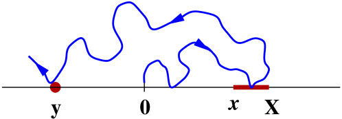
Figure 6: Two interval zig-zag probability.

We shall identify $Q_{2}(x,X;y)$ with a particular CFT correlation function which involves a primary field $\Psi_{1;3}$ of weight $h_{1;3}$ localized on the infinitesimal interval $[y,y+dy]$ and two primary fields $\Psi_{0}$ of weight zero localized at the end points of the macroscopic interval $[x,X]$.

So let us consider the correlation function

$$F(X,x;y)\equiv\langle\omega|\Psi_{0}(X){}_{[1;2]}\,\Psi_{0}(x){}_{[1;4]}\,\Psi_{1;3}(y)|\omega\rangle$$ (28)

The intermediate indices _[1;2] and _[1;4] refer to the conformal weights of the Virasoro representations which propagate in the intermediate channels, eg. $\Psi_{1;3}(y)$ in the above formula is the primary field of dimension $h_{1;3}$ intertwining Virasoro modules of weights $h_{1;2}$ and $h_{1;4}$. By the CFT fusion rules, which are consequences of the null vector relation $(L_{-2}-\frac{\kappa}{4}L_{-1}^{2})|\omega\rangle=0$, in the correlation function (28), the intermediate representation between the dimension zero operators $\Psi_{0}(X)$ and $\Psi_{0}(x)$ could only have weight $h_{1;0}$ or $h_{1;2}$ – and we choose $h_{1;2}$ – whereas the intermediate representation between $\Psi_{0}(x)$ and $\Psi_{1;3}(y)$ could only have weight $h_{1;2}$ or $h_{1;4}$ – and we choose $h_{1;4}$ there. Choosing these representations amounts to select a particular conformal block.

We are going to argue (i) that, up to a proportionality coefficient, $F(X,x;y)$ satisfies the same boundary conditions (27) as $Q_{2}(x,X;y)$ – and this is how we have chosen the intermediate channels, and (ii) that, up to the same proportionality coefficient, it is such that

$$F\Big{(}f_{\tau}(X),f_{\tau}(x);f_{\tau}(y)\Big{)}\,|f^{\prime}_{\tau}(y)|^{h_{1;3}}={\rm const.}\,{\bf 1}_{\tau_{x}<\tau_{X}}\ {\bf 1}_{\tau_{x}<\tau_{y}}\ \Big{|}{\frac{f^{\prime}_{\tau_{x}}(y)}{f_{\tau_{x}}(y)}}\Big{|}^{h_{1;3}}$$ (29)

for $\tau=\min(\tau_{x},\tau_{y})$. This will follow from the fact that $F(x,X;y)$ satisfies the boundary conditions (27). Since by the martingale property, we know that

$${\bf E}[\,F\Big{(}f_{\tau}(X),f_{\tau}(x);f_{\tau}(y)\Big{)}\,|f^{\prime}_{\tau}(y)|^{h_{1;3}}\,]=F(X,x;y),$$

this will imply that $F(X,x;y)={\rm const.}\,Q_{2}(y;x,X)$, where ${\rm const.}$ is the above mentioned proportionality coefficient.

Let us first look at the boundary conditions. Consider the limit $y\to 0$. By CFT fusion rules, the operator $\Psi_{1;3}(y)$ maps $|\omega\rangle$ in a Virasoro module of weight $h_{1;2}$ or $h_{1;4}$. Demanding that $\Psi_{1;3}(y)|\omega\rangle$ vanishes as $y\to 0$ selects the image space to be of Virasoro weight $h_{1;4}$, because then $\Psi_{1;3}(y)|\omega\rangle\simeq y^{4/\kappa}|h_{1;4}\rangle+\cdots$, without contribution from the $h_{1;2}$ module which would be divergent. This fixes the intermediate channel between $\Psi_{0}(x)$ and $\Psi_{1;3}(y)$ to be _[1;4].

To fix the other intermediate channel we look at the limit $x\to 0$. In this limit, $x$ is approaching the localization point of $|\omega\rangle$, so we have to exchange the order by which we act with $\Psi_{0}(x)$ and $\Psi_{1;3}(y)$ using the CFT braiding relations:

$$\Psi_{0}(x){}_{[1;4]}\,\Psi_{1;3}(y)|\omega\rangle=B_{[1;4]}^{[1;2]}\ \Psi_{1;3}(y){}_{[1;2]}\,\Psi_{0}(x)|\omega\rangle+B_{[1;4]}^{[1;0]\ }\Psi_{1;3}(y){}_{[1;0]}\,\Psi_{0}(x)|\omega\rangle$$

There are only two contributions to this braiding relation because of the fusion rules implied by the level two null vector $(L_{-2}-\frac{\kappa}{4}L_{-1}^{2})|\omega\rangle=0$. In the limit $x\to 0$, the first term dominates and $\Psi_{0}(x){}_{[1;4]}\,\Psi_{1;3}(y)|\omega\rangle\simeq B_{[1;4]}^{[1;2]}\ \Psi_{1;3}(y)|\omega\rangle+\cdots$. This gives, as $x\to 0$,

$$\langle\omega|\Psi_{0}(X)\Psi_{0}(x){}_{[1;4]}\,\Psi_{1;3}(y)|\omega\rangle\simeq B_{[1;4]}^{[1;2]}\ \langle\omega|\Psi_{0}(X)\Psi_{1;3}(y)|\omega\rangle+\cdots$$

The boundary condition (27) demands the above r.h.s. be proportional to $|y|^{-h_{1;3}}$ for all $X$. This fixes the intermediate representation between $\Psi_{0}(X)$ and $\Psi_{1;3}(y)$ to be of weight $h_{1;2}$ and not $h_{1;0}$, because $\langle\omega|\Psi_{0}(X){}_{[1;2]}\Psi_{1;3}(y)|\omega\rangle=|y|^{-h_{1;3}}$ for all $X$.

The last boundary condition for $X\to x$ is again a consequence of the fusion relation of the dimension zero operators:

$$\langle\omega|\Psi_{0}(X){}_{[1;2]}\Psi_{0}(x){}_{[1;4]}\simeq(X-x)^{h_{1;3}}\,\langle\omega|\Psi_{1;3}(x){}_{[1;4]}+\cdots$$

Only the operators $\Psi_{1;3}$ and $\Psi_{1;5}$ may appear in this fusion, and the $\Psi_{1;3}$ contribution is dominant as $X\to x$.

Let us now show that these boundary conditions imply that $F(X,x;y)$ satisfies eq.(29). We have to distinguish the three topologically distinct configurations: (i) $\tau_{y}<\tau_{x}\leq\tau_{X}$, (ii) $\tau_{x}=\tau_{X}<\tau_{y}$ and (iii) $\tau_{x}<\tau_{y}$ and $\tau_{x}<\tau_{X}$. In case (i), point $y$ is swallowed before $x$ and $X$, thus $\tau=\tau_{y}$ and $f_{\tau}(y)\to 0$ with $f_{\tau}(x)$ and $f_{\tau}(X)$ finite. The first boundary condition (27) then implies that $F(f_{\tau}(X),f_{\tau}(x);f_{\tau}(y))\,|f^{\prime}_{\tau}(y)|^{h_{1;3}}$ vanishes. In case (ii), points $x$ and $X$ are swallowed simultaneously before $y$, so $\tau=\tau_{x}$ and $(f_{\tau}(x)-f_{\tau}(X))\to 0$ faster that $f_{\tau}(x)$ and $f_{\tau}(X)$ while $f_{\tau}(y)$ remains finite. The third boundary condition (27) implies that $F(f_{\tau}(X),f_{\tau}(x);f_{\tau}(y))\,|f^{\prime}_{\tau}(y)|^{h_{1;3}}$ also vanishes in this case. In case (ii), the SLE trace touches the interval $[x,X]$ before swallowing $y$, hence $\tau=\tau_{x}$ and $f_{\tau}(x)\to 0$ with $f_{\tau}(X)$ and $f_{\tau}(y)$ finite. The second boundary condition (27) then implies that $F(f_{\tau}(X),f_{\tau}(x);f_{\tau}(y))\,|f^{\prime}_{\tau}(y)|^{h_{1;3}}$ is equal to $|f^{\prime}_{\tau_{x}}(y)/f_{\tau_{x}}(y)|^{h_{1;3}}$. This proves eq.(29) and hence $F(X,x;y)={\rm const.}\,Q_{2}(y;x,X)$.

We can now go on and look for the density probability of hitting two infinitesimal intervals, say on both side of the origin, touching first $[x,x+dx]$ and then $[y,y+dy]$ with $y<0<x$:

$$P_{2}([x,x+dx];[y,y+dy])\equiv Q_{2;2}(x;y)\,(dy)^{h_{1;3}}(dx)^{h_{1;3}}$$

This may be obtained from eq.(28) by fusing the weight zero primary operators as above: $\langle\omega|\Psi_{0}(X){}_{[1;2]}\Psi_{0}(x){}_{[1;4]}\simeq C_{1}(X-x)^{h_{1;3}}\,\langle\omega|\Psi_{1;3}(x){}_{[1;4]}+\cdots$. We get, up to a proportionality coefficient:

$$Q_{2;2}(x;y)={\rm const.}\,\langle\omega|\Psi_{1;3}(x){}_{[1;4]}\Psi_{1;3}(y)|\omega\rangle$$

where, again, the index _[1;4] specifies the intermediate channel. It satisfies a hypergeometric differential equation and it may thus be written in terms of hypergeometric function. The explicit formula, although easy to obtain, is not very useful at this point. This correlation function may also be identified, up to a proportionality coefficient, with

$${\bf E}[{\bf 1}_{\tau_{x}<\tau_{y}}\Big{|}\frac{f^{\prime}_{\tau_{x}}(x)f^{\prime}_{\tau_{x}}(y)}{f_{\tau_{x}}(x)f_{\tau_{x}}(y)}\Big{|}^{h_{1;3}}].$$

This shows that each infinitesimal interval counts for the insertion of a factor $\big{|}f^{\prime}_{\tau}(x)/f_{\tau}(x)\big{|}^{h_{1;3}}$ in the SLE expectation or for the insertion of the boundary primary field $\Psi_{1;3}$ in the CFT correlation functions.

This example illustrate how zig-zag probabilities of SLE paths may be identified with CFT correlation functions. It shows that fusion algebras of CFT are at the heart of this identification.

Other examples dealing with more intervals, in various side of the origin and visited by the SLE path in various order, may be considered. However, the identification of the appropriate CFT correlation functions which will code for these zig-zag probabilities becomes more and more involved. For instance, it is clear that probabilities that the SLE path touches infinitesimal intervals are given by correlation functions of $\Psi_{1;3}$ operators and that specifying the order in which these intervals are visited selects the appropriate conformal block. But we didn’t find any simple rule encompassing all cases.

9 Bulk zig-zag probabilities.

Bulk zig-zag probabilities are probabilities for the SLE curve to visit a set of balls on the upper half plane in a given order. The following is essentially a reformulation, using CFT approach, of Beffara’s proof [11] that the fractal dimension of a SLE curve is $d_{\kappa}=1+\kappa/8$ for $\kappa\leq 8$ and $d_{\kappa}=2$ for $\kappa\geq 8$, a formula which was conjectured by Duplantier [12].

9.1 Fractal dimension and one-point function.

The fractal dimension $d_{\kappa}$ may be evaluated by using a one point estimate, namely the probability that the SLE path approaches a point $z_{0}$ in the bulk of the upper half plane at a distance less that $\varepsilon$:

$${\bf P}[\gamma_{[0,+\infty)}\cap\mathbb{B}_{\varepsilon}(z_{0})\not=\emptyset]\approx\varepsilon^{2-d_{\kappa}},\quad\varepsilon\to 0$$

with $\mathbb{B}_{\varepsilon}(z_{0})$ the ball of radius $\varepsilon$ centered in $z_{0}$. This yields [12, 11]: $d_{\kappa}=2-2h_{0;1}=1+\kappa/8$ for $\kappa<8$.

The complete determination of $d_{\kappa}$ requires also establishing a two point estimate, which is much harder to obtain but which may be found in the nice reference [11].

Let $z_{0}\in\mathbb{H}$, $\Im{\rm m}z_{0}>0$, be a point in the upper half plane and $\delta_{t}(z_{0})$ its distance to the SLE curve $\gamma_{[0,t]}$ stopped at time $t$. We shall evaluate $\delta_{t}(z_{0})$ using the conformal radius of $\gamma_{[0,t]}$ seen from $z_{0}$. Let $h_{t}(z)$, defined by

$$h_{t}(z)=\frac{g_{t}(z)-g_{t}(z_{0})}{g_{t}(z)-\overline{g_{t}(z_{0})}}$$

be a uniformizing map of $\mathbb{H}\setminus\mathbb{K}_{t}$ onto the unit disk with $h_{t}(z_{0})=0$, $h_{t}(\infty)=1$. It maps the tip of the curve on the unit circle, $U_{t}\equiv h_{t}(\gamma(t))\in\mathbb{S}_{1}$, with $U_{t}=f_{t}(z_{0})/\overline{f_{t}(z_{0})}\equiv e^{i\alpha_{t}}$. This defines a process $\alpha_{t}$ on the unit circle with $\alpha_{t}\to 0$ or $2\pi$ as $t\to\tau_{z_{0}}$ depending whether $z_{0}$ has been swallowed clockwise, or counterclockwise, by the SLE trace. Actually, up to a random time reparametrization, $ds=(\frac{2\Im{\rm m}f_{t}(z_{0})}{|f_{t}(z_{0})|^{2}})^{2}dt$, this process is driven by $d\alpha_{s}=\frac{\kappa-4}{4}\cot(\alpha_{s}/2)+d\xi_{s}$.

The conformal radius of $\gamma_{[0,t]}$ viewed from $z_{0}$ is defined as $\rho_{t}(z_{0})\equiv|h_{t}^{\prime}(z_{0})|^{-1}$. An explicit computation shows that $\rho_{t}(z_{0})=|2\Im{\rm m}f_{t}(z_{0})/f^{\prime}_{t}(z_{0})|$. Köbe $1/4$-theorem states that $\delta_{t}(z_{0})$ and $\rho_{t}(z_{0})$ scale the same way, since $(1/4)\rho_{t}(z_{0})\leq\delta_{t}(z_{0})\leq\rho_{t}(z_{0})$. One may check that $\rho_{t}(z_{0})$ is always decreasing as time goes by. So instead of estimating the distance between the SLE path and $z_{0}$, we shall estimate its conformal radius, $\rho(z_{0},\gamma)=\lim_{t\to\tau_{z_{0}}}\rho_{t}(z_{0})$, and the probability

$${\bf P}[\rho(z_{0},\gamma)\leq\varepsilon]$$ (30)

Estimating ${\bf P}[\rho(z_{0},\gamma)\leq\varepsilon]$ can be formulated [11] as a survival probability problem for the process $\alpha_{s}$ but, in order to understand its CFT origin, we shall compute it using our favorite martingale $G_{t}|\omega\rangle$. For $\kappa<8$, let us consider the expectation value

$$\hat{M}_{t}(z_{0})\equiv\langle\omega|\Phi_{0;1}(z_{0},\bar{z}_{0})G_{t}|\omega\rangle$$

with $\Phi_{0;1}$ the bulk conformal field of weight $2h_{0;1}=(8-\kappa)/8$. By construction this is well defined up to time $t<\tau_{z_{0}}$. The correlation function $\langle\omega|\Phi_{0;1}(z_{0},\bar{z}_{0})|\omega\rangle$ may be computed exactly using the level two null vector. It is equal to

$$|2\Im{\rm m}z_{0}|^{-2h_{0;1}}(\sin\alpha_{0}/2)^{\kappa/8-1}$$

with $z_{0}/\bar{z}_{0}=e^{i\alpha_{0}}$ so that

$$\hat{M}_{t}(z_{0})=\Big{|}\frac{f^{\prime}_{t}(z_{0})}{2\Im{\rm m}f_{t}(z_{0})}\Big{|}^{2h_{0;1}}\,(\sin\alpha_{t}/2)^{\kappa/8-1}=\rho_{t}(z_{0})^{-2h_{0;1}}\,(\sin\alpha_{t}/2)^{\kappa/8-1}$$

Let $\theta_{z_{0}}^{\varepsilon}$ be either the time at which the conformal radius $\rho_{t}(z_{0})$ reaches the value $\varepsilon$, if $\rho(z_{0},\gamma)\leq\varepsilon$, or the swallowing time $\tau_{z_{0}}$ if the point $z_{0}$ is swallowed before the conformal radius reaches this value, i.e. if $\rho(z_{0},\gamma)>\varepsilon$. The time $\theta_{z_{0}}^{\varepsilon}$ is a stopping time. Since $f^{\prime}_{t}(z_{0})$ vanishes faster than $f_{t}(z_{0})$ as $t\to\tau_{z_{0}}$, the martingale $\hat{M}_{t}(z_{0})$ vanishes as $t\to\tau_{z_{0}}$ for $\kappa<8$. Therefore it projects on

$$\hat{M}_{\theta_{z_{0}}^{\varepsilon}}(z_{0})=\varepsilon^{-2h_{0;1}}\,(\sin\alpha_{\theta_{z_{0}}^{\varepsilon}}/2)^{\kappa/8-1}\ {\bf 1}_{\rho(z_{0},\gamma)\leq\varepsilon}$$

By construction $\hat{M}_{t}(z_{0})$ is a martingale so that ${\bf E}[\hat{M}_{\theta_{z_{0}}^{\varepsilon}}(z_{0})]=\hat{M}_{t=0}(z_{0})$, or, using the basic definition of conditional probability,

$${\bf P}[\rho(z_{0},\gamma)\leq\varepsilon]\ \cdot\ {\bf E}[(\sin\alpha_{\theta_{z_{0}}^{\varepsilon}}/2)^{\kappa/8-1}\,|\,\rho(z_{0},\gamma)\leq\varepsilon]$$

$$\hskip 28.45274pt=\Big{(}\frac{\varepsilon}{2\Im{\rm m}z_{0}}\Big{)}^{2h_{0;1}}\ (\sin\alpha_{0}/2)^{\kappa/8-1}$$

The conditional probability ${\bf E}[(\sin\alpha_{\theta_{z_{0}}^{\varepsilon}}/2)^{\kappa/8-1}\,|\,\rho(z_{0},\gamma)\leq\varepsilon]$ is bounded so that ${\bf P}[\rho(z_{0},\gamma)\leq\varepsilon]\approx\varepsilon^{2h_{0;1}}$ as $\varepsilon\to 0$. This gives the one point estimate (30) and the fractal dimension $d_{\kappa}=2-2h_{0;1}$.

9.2 Bulk zig-zags and $N$-point functions.

The previous computation indicates that the operator testing for the emergence of two SLE paths from a tiny ball in $\mathbb{H}$ is the bulk primary field $\Phi_{0;1}$.

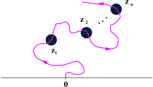
Figure 7: Bulk zig-zag probabilities.

As in Figure(7), one may look for the zig-zag density probability that the SLE path visit balls $\mathbb{B}_{\varepsilon}(z_{p})$, $\varepsilon\to 0$, centered in points $z_{p}$,

$$\lim_{\varepsilon\to 0}\varepsilon^{-2nh_{0;1}}\,{\bf P}[\gamma_{[0,\infty)}\ {\rm visits}\ B_{\varepsilon}(z_{1})\cup\cdots\cup B_{\varepsilon}(z_{n})]$$

in the order $z_{1},\cdots,z_{n}$. This is clearly proportional to a CFT correlation functions of field of dimension $h_{0;1}$:

$$\langle\omega|\Phi_{0;1}(z_{1},\bar{z}_{1})\cdots\Phi_{0;1}(z_{n},\bar{z}_{n})|\omega\rangle$$

As in the boundary case, to define these correlation functions one has to specify the Virasoro representations propagating in the intermediate channels.

If no order among the visited balls is specified, these correlation functions have no monodromy and they thus correspond to the complete $\Phi_{0;1}$ CFT correlation functions. Zig-zag probabilities with specified ordering in the visits would probably be exchanged as one moves the points $z_{p}$ around. In other words, there is probably a quite direct relation between CFT monodromies, alias quantum groups, and braiding properties of samples of SLE traces.

Acknowledgments:

Work supported in part by EC contract number HPRN-CT-2002-00325 of the EUCLID research training network.

References

- [1] A. Belavin, A. Polyakov and A. Zamolodchikov, Nucl. Phys. B241, 333-380, (1984).
- [2] O. Schramm, Israel J. Math., 118, 221-288, (2000);
- [3] S. Rhode and O. Schramm, Basic properties of SLE, arXiv: math.PR/0106036; and references therein.
-
[4]
G. Lawler, O. Schramm and W. Werner,
(I): Acta Mathematica 187 (2001) 237-273; arXiv:math.PR/9911084
G. Lawler, O. Schramm and W. Werner, (II): Acta Mathematica 187 (2001) 275-308; arXiv:math.PR/0003156
G. Lawler, O. Schramm and W. Werner, (III): Ann. Henri Poincaré 38 (2002) 109-123. arXiv:math.PR/0005294. - [5] G. Lawler, O. Schramm and W. Werner, Conformal restriction: the chordal case, arXiv:math.PR/0209343.
- [6] G. Lawler, introductory texts, including the draft of a book, may be found at http://www.math.cornell.edu/lawler
- [7] M. Bauer and D. Bernard, Commun. Math. Phys. 239 (2003) 493-521, arXiv:hep-th/0210015, and Phys. Lett. B543 (2002) 135-138, arXiv:math-ph/0206028.
- [8] M. Bauer and D. Bernard, Phys. Lett. B557 (2003) 309-316, arXiv:hep-th/0301064.
- [9] M. Bauer and D. Bernard, Conformal transformations and the SLE partition function martingale, arXiv:math-ph/0305061.
- [10] R.Friedrich and W. Werner, Conformal restriction, highest weight representations and SLE, arXiv:math-ph/0301018.
- [11] V. Beffara, The dimension of the SLE curves, arXiv:math.PR/0211322.
- [12] B. Duplantier, Conformal fractal geometry and boundary quantum gravity, arXiv:math-ph/0303034, and references therein.
- [13] J. Cardy, J. Phys. A25, L201-206, (1992).
- [14] N. Makarov, seminar at IHP-Paris, 2002, unpublished.
- [15] D. Zhan, Stochastic Loewner evolution in doubly connected domains, arXiv:math.PR/031035.
- [16] R. Friedrich and J. Kalkkinen, On Conformal Field Theory and Stochastic Loewner Evolution, arXiv:hep-th/0308020.
- [17] J. Dubédat, Critical percolation in annuli and , arXiv: math.PR/0306056.
- [18] M. Bauer and D. Bernard, CFTs of SLEs : the radial case, arXiv:math-ph/0310032.