The uses of random partitions

Abstract

These are extended notes for my talk at the ICMP 2003 in Lisbon. Our goal here is to demonstrate how natural and fundamental random partitions are from many different points of view. We discuss various natural measures on partitions, their correlation functions, limit shapes, and how they arise in applications, in particular, in the Gromov-Witten and Seiberg-Witten theory.

1 Recognizing random partitions

1.1 Why partitions ?

1.1.1

Random partitions occur in mathematics and physics in a wide variety of contexts. For example, a partition can record a state of some random growth process. More often it happens that a certain quantity of interest is expressed, explicitly or implicitly, as a sum over partitions. This can come as a result of a localization computation in geometry, or from a character expansion of a matrix integral, or from something as innocent as expanding a determinant. Typically, one can recognize in such a sum a discrete version of some random matrix integral and so one can ask whether the powerful and honed tools of the random matrix theory can be applied.

The purpose of these notes is to argue that certain natural measures on partitions are not just discrete caricatures of random matrix ensembles, but are, in fact, objects of fundamental importance, with profound connections to many central themes of mathematics and physics, including, in particular, integrable systems. Therefore, I believe that it is very natural to present these views in this special session on Random Matrix Theory and Integrable Systems.

1.1.2

The wealth of applications and connections of random matrices is such that it is utterly impossible to argue that something is “just as good” in one short talk. So, instead of trying to paint the whole picture, I will give a few illustrative examples, selected according to my own limited expertise and taste. Much, much more can be found in the works cited in the bibliography. But even though I tried to make the bibliography rather extensive, it is still hopelessly far from being complete.

Several topics that should be covered in any reasonable survey on random partitions are completely omitted here. These include, for example, the 2-dimensional Yang-Mills theory and character expansions in the random matrix theory. We also say nothing about the relation between random partitions and planar dimer models, even though the 2-dimensional point of view on random partitions if often illuminating, has several technical advantages, as well as some exciting connections to algebraic geometry [44].

1.2 Coordinates on partitions

1.2.1 Diagram of a partition

By definition, a partition $\lambda$ is simply a monotone sequence

$$\lambda=(\lambda_{1}\geq\lambda_{2}\geq\lambda_{3}\geq\dots\geq 0)$$

of nonnegative integers such that $\lambda_{i}=0$ for $i\gg 0$. The size of $\lambda$ is, by definition, the number $|\lambda|=\sum\lambda_{i}$.

The standard geometric object associated to a partition is its diagram. There are several competing traditions of drawing the diagram. We will follow the one illustrated in Fig. 1,

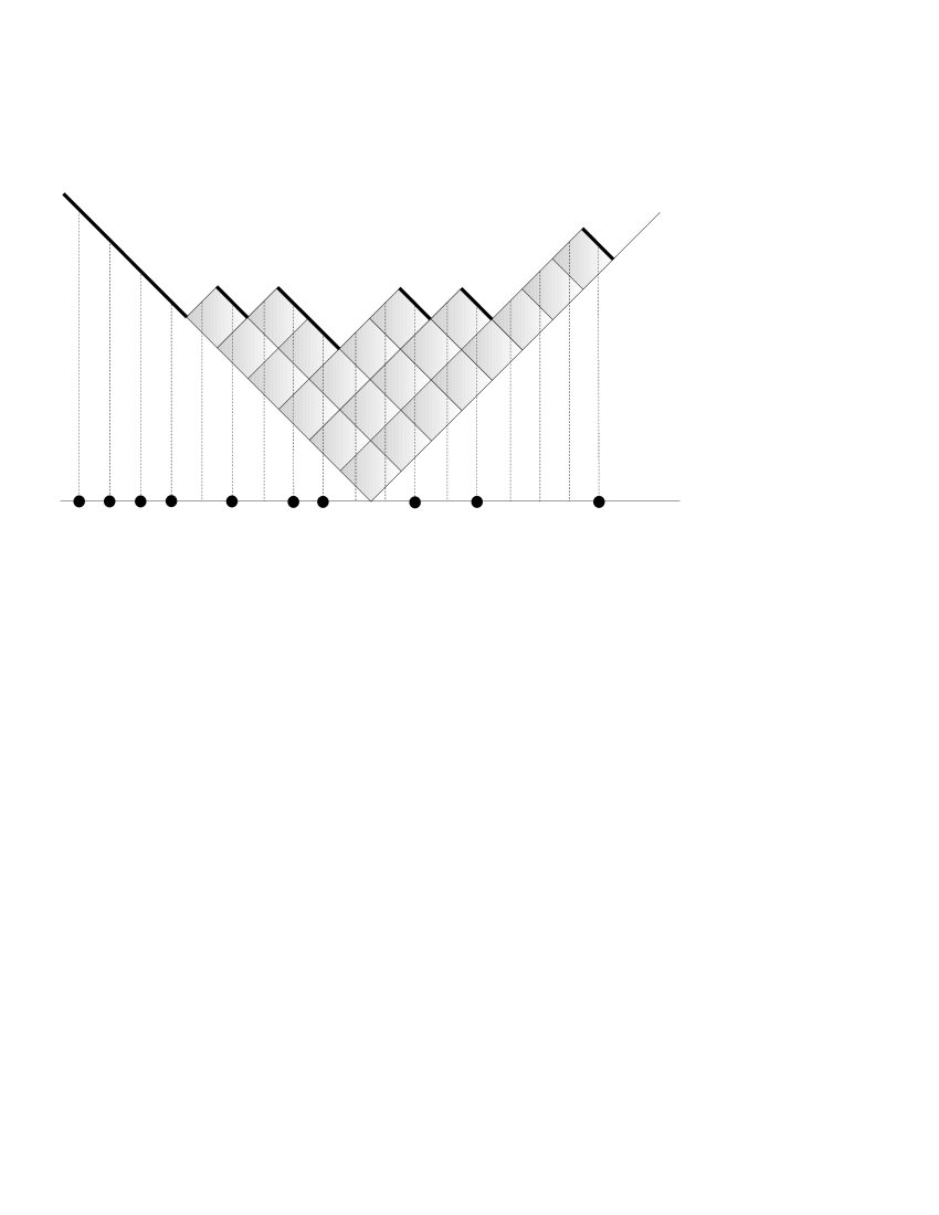
Figure 1: The partition $(8,5,4,2,2,1)$

which portrays the partition $\lambda=(8,5,4,2,2,1)$. This way of drawing diagrams is sometimes referred to as the Russian one (as opposed to the older French and English traditions of drawing partitions). Its advantages are not just that the picture looks more balanced on the page and saves space by a factor of $\approx\sqrt{2}$, but also that from it one can see more clearly several other useful ways of parameterizing the partitions.

1.2.2 Profile of a partition

The upper boundary in Fig. 1 is a graph of a function $f_{\lambda}(x)$ such that $f^{\prime}_{\lambda}(x)=\pm 1$. This function $f_{\lambda}$ is known as the profile of the partition $\lambda$. The map $\lambda\mapsto f_{\lambda}$ from partitions to functions with Lipschitz constant $1$ allows one to talk about limit shape of partitions. Namely, given a sequence of probability measures on partitions, we say that it has a limit shape $f$ if, after a suitable scaling, the corresponding measures on functions converge weakly to the $\delta$-measure on $f$.

1.2.3 Partitions vs. particles

Another useful way to parametrize partitions is via the map

$$\mathfrak{S}:\lambda\mapsto\left\{\lambda_{i}-i+\frac{1}{2}\right\}\subset\mathbb{Z}+\frac{1}{2}$$

from partitions to subsets of $\mathbb{Z}+\frac{1}{2}$. The geometric meaning of the set $\mathfrak{S}(\lambda)$ should be clear from Fig. 1 where the elements of $\mathfrak{S}(\lambda)$ are shown by bold dots. The map $\mathfrak{S}$ makes a random partition a random subset of $\mathbb{Z}+\frac{1}{2}$ or, in other words, an ensemble of random particles on the lattice. It is these random particles that are the analogs of eigenvalues of a random matrix. A natural question here is to compute the correlation functions, that is, the probability to observe particles in specified locations.

1.3 Partitions and the fermionic Fock space

1.3.1 Subspaces instead of subsets

Note that, for any partition $\lambda$, the set $\mathfrak{S}(\lambda)$ has as many positive elements as it has negative holes (that is, negative half-integers not in $\mathfrak{S}(\lambda)$). It can be viewed, therefore, as a finite excitation over the Dirac sea

$$\mathfrak{S}(\emptyset)=\left\{-1/2,-3/2,-5/2,\dots\right\}\,,$$

in which all negative positions are filled by particles while all positive ones are vacant.

Consider the vector space $V$ with an orthonormal basis $\{e_{k}\}$, $k\in\mathbb{Z}+\frac{1}{2}$, indexed by all possible positions of one particle. To a partition $\lambda$ one then associated the following vector

$$v_{\lambda}=e_{\lambda_{1}-\frac{1}{2}}\wedge e_{\lambda_{2}-\frac{3}{2}}\wedge e_{\lambda_{3}-\frac{5}{2}}\wedge\dots$$

in the half-infinite exterior power ${\bigwedge}^{\!\frac{\infty}{2}}V$ of the $1$-particle space $V$. In other words, one associates to a partition $\lambda$ the image of the subspace spanned by $\{e_{k}\}$, $k\in\mathfrak{S}(\lambda)$, under the Plücker embedding of the corresponding Grassmannian.

Note that the vectors $v_{\lambda}$ are orthonormal with respect to the natural inner product, and, in particular, any vector $v$ in their span defines a probability measure measure $\mathfrak{M}_{v}$ on partitions by

$$\mathfrak{M}_{v}(\lambda)=\frac{|(v,v_{\lambda})|^{2}}{\|v\|^{2}}\,.$$ (1.1)

1.3.2 The action of $GL(\infty)$

The main advantage of trading sets for linear spaces like we just did is the following. The group $GL(V)$ of invertible linear transformations of a finite-dimensional vector space $V$ acts naturally in all exterior powers of $V$. The case of an infinite exterior power of an infinite-dimensional space requires more care (in particular, the need for normal ordering of operators arises), but it is still possible to define a projective action on ${\bigwedge}^{\!\frac{\infty}{2}}V$ of a suitable version of the group $GL(V)$, see for example [42, 60, 81].

For our purposes, it suffices to define the action of the operators of the form $e^{X}$, where the matrix $X$ lies in the Lie algebra $\mathfrak{gl}(V)$. If $X$ has zeros on the diagonal then the naive definition of its action on ${\bigwedge}^{\!\frac{\infty}{2}}V$ works fine (note however, that a central extension appears, see e.g. (1.9)). For diagonal matrices $X$, we will use the formula (2.9) as our regularization recipe.

It is the gigantic symmetry group $GL(V)$ that makes certain computations in ${\bigwedge}^{\!\frac{\infty}{2}}V$ so pleasant (such as, for example, computations of correlation functions, see below). It also opens up the connection to integrable systems, where, through the work of the Kyoto school and others, the space ${\bigwedge}^{\!\frac{\infty}{2}}V$ has become one of the cornerstones of the theory.

1.4 Plancherel measure

We conclude this introductory section with the discussion of the most basic measure on the set of partitions — the Plancherel measure.

1.4.1 Representation theory

The general linear group and the symmetric group $S(n)$ are the two most important groups in mathematics and the representation theory of both groups is saturated with partitions. In particular, over a field of characteristic zero (we will not come across any other fields in these notes), irreducible representations of $S(n)$ are indexed by partitions $\lambda$ of size $n$. Let $\dim\lambda$ denote the dimension of the corresponding representation. It follows from a theorem of Burnside that the formula

$$\mathfrak{M}_{\textup{Planch}}(\lambda)=\frac{(\dim\lambda)^{2}}{n!}$$ (1.2)

defines a probability measure on the set of partitions of $n$. This measure is known as the Plancherel measure, because of its relation to the Fourier transform on the group $S(n)$.

Often, it is more convenient to consider a related measure on the set of all partitions defined by

$$\mathfrak{M}_{\textup{PP}}(\lambda)=e^{-\xi}\,\xi^{|\lambda|}\,\left(\frac{\dim\lambda}{|\lambda|!}\right)^{2}\,,\quad\xi>0\,.$$ (1.3)

It is known as the poissonized Plancherel measure, the number $\xi>0$ being the parameter of the poissonization.

1.4.2 Plancherel and GUE

While representation theory provides an important motivation for the study of the Plancherel measure, the representation–theoretic definition of it may sound like something very distant from the “real world” until one recognizes, through other interpretations of the number $\dim\lambda$, that one is dealing here with a distinguished discretization of the GUE ensemble from the random matrix theory. S. Kerov (see, for example his book [50]) and K. Johansson [38] were among the first to recognize this connection.

A pedestrian way to see the connection to the GUE ensemble is to use the following formula

$$\dim\lambda=\frac{|\lambda|!}{\prod(\lambda_{i}+k-i)!}\,\prod_{i<j\leq k}(\lambda_{i}-\lambda_{j}+j-i)\,,$$ (1.4)

where $k$ is any number such that $\lambda_{k+1}=0$. The first factor in (1.4) is roughly a multinomial coefficient and hence a discrete analog of the Gaussian weight, while the second factor looks like Vandermonde determinant in the variables $\mathfrak{S}(\lambda)$. This makes $(\dim\lambda)^{2}$ resemble the radial part of the GUE measure given, up to a constant factor, by the weight

$$e^{-\frac{1}{2}\sum x_{i}^{2}}\prod_{i<j\leq N}(x_{i}-x_{j})^{2}\,,$$ (1.5)

the particles $\mathfrak{S}(\lambda)$ playing the role of the eigenvalues $\{x_{i}\}$.

1.4.3 Plancherel measure and random growth

Another interpretation of $\dim\lambda$ is the following: it is the number of ways to grow the diagram of $\lambda$ from the empty diagram $\emptyset$ by adding a square at a time, while maintaining a partition at every step. For example, $\dim(2,2)=2$ corresponds to the two possible growth histories shown in Fig. 2.

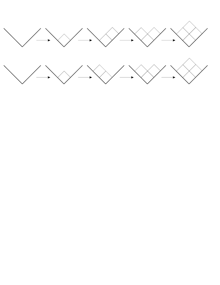
Figure 2: The two ways to grow the partition $(2,2)$

In representation theory, this interpretation of $\dim\lambda$ is a consequence of the branching rule for the restriction $S(n)\downarrow S(n-1)$. It links Plancherel measure with the Robinson-Schensted algorithm (see, for example, [12, 84]) and many related growth processes.

In particular, by a theorem of Schensted, the distribution of $\lambda_{1}$ with respect to $\mathfrak{M}_{\textup{Planch}}$ is precisely the distribution of the longest increasing subsequence in a uniformly random permutation of $\{1,\dots,n\}$. The understanding of this distribution was a major stimulus for the study of Plancherel measure, culminating in the work of J. Baik, P. Deift, and K. Johansson [3]. They proved that the scaled and centered distribution of $\lambda_{1}$ converges to the Tracy-Widom distribution [85] which describes the maximal eigenvalue of a large random Hermitian matrix. They also proved a similar statement for $\lambda_{2}$ and conjectured that, more generally, the joint distribution of $\{\lambda_{1},\lambda_{2},\dots\}$, scaled and centered, converges to the Airy ensemble which describes the behavior of the $1$st, $2$nd, and so on eigenvalues of a large random matrix. This conjecture was established in [68, 8, 39], see more in Section 4.2.2 below.

Plancherel measure also arises in more general growth processes, where both adding and removing a square is allowed, see below. This is a discrete analog of how one finds the GUE distribution in the context of non-intersecting Brownian motions, see for example [40].

1.4.4 Operator form of partition growth

Consider the following elements of the Lie algebra $\mathfrak{gl}(V)$

$$\alpha_{n}\cdot e_{k}=e_{k-n}\,.$$ (1.6)

From definitions, one finds that in the basis $v_{\lambda}$ the operator $\alpha_{-1}$ acts as follows

$$\alpha_{-1}\cdot v_{\lambda}=\sum_{\mu=\lambda+\square}v_{\mu}\,,$$ (1.7)

where the summation is over all possibilities to add a square to the partition $\lambda$. Exponentiating (1.7) and comparing it to (1.1), we conclude that $\mathfrak{M}_{PP}=\mathfrak{M}_{v}$, where

$$v=\exp\left(\sqrt{\xi}\,\alpha_{-1}\right)\cdot v_{\emptyset}\,.$$ (1.8)

Similarly, the adjoint operator $\alpha_{1}=\alpha_{-1}^{*}$ removes a square from partitions. From the basic commutation relation

$$\left[\alpha_{n},\alpha_{m}\right]=n\,\delta_{n+m}$$ (1.9)

satisfied by the operators $\alpha_{n}$ in the (projective) representation ${\bigwedge}^{\!\frac{\infty}{2}}V$, one sees that mixing adding squares with removing squares leads again to the Plancherel measure.

The formula (1.8) leads to a simple computation of the correlation function of the Plancherel measure, see below.

2 Random partitions in Gromov-Witten theory

2.1 Random matrices and moduli of curves

2.1.1 Matrix integrals in 2D quantum gravity

The Wick formula expansion of the following Gaussian integral over the space of $N\times N$ Hermitian matrices $H$

$$\int e^{-\frac{1}{2}\operatorname{tr}H^{2}}\prod_{i=1}^{n}\operatorname{tr}H^{k_{i}}\,dH=\textup{const}\int_{\mathbb{R}^{N}}e^{-\frac{1}{2}\sum x_{i}^{2}}\prod_{i<j}(x_{i}-x_{j})^{2}\prod_{i=1}^{n}\left(\sum_{j=1}^{N}x_{j}^{k_{i}}\right)\,dx$$ (2.1)

is well-known to enumerate different ways to glue an orientable surfaces of a given genus $g$ from a $k_{1}$-gon, $k_{2}$-gon, etc., see for example [94] for an elementary introduction. In other words, the integral (2.1) can be written as a certain sum over discretized surfaces, also known as maps on surfaces, of the kind shown in Fig. 3.

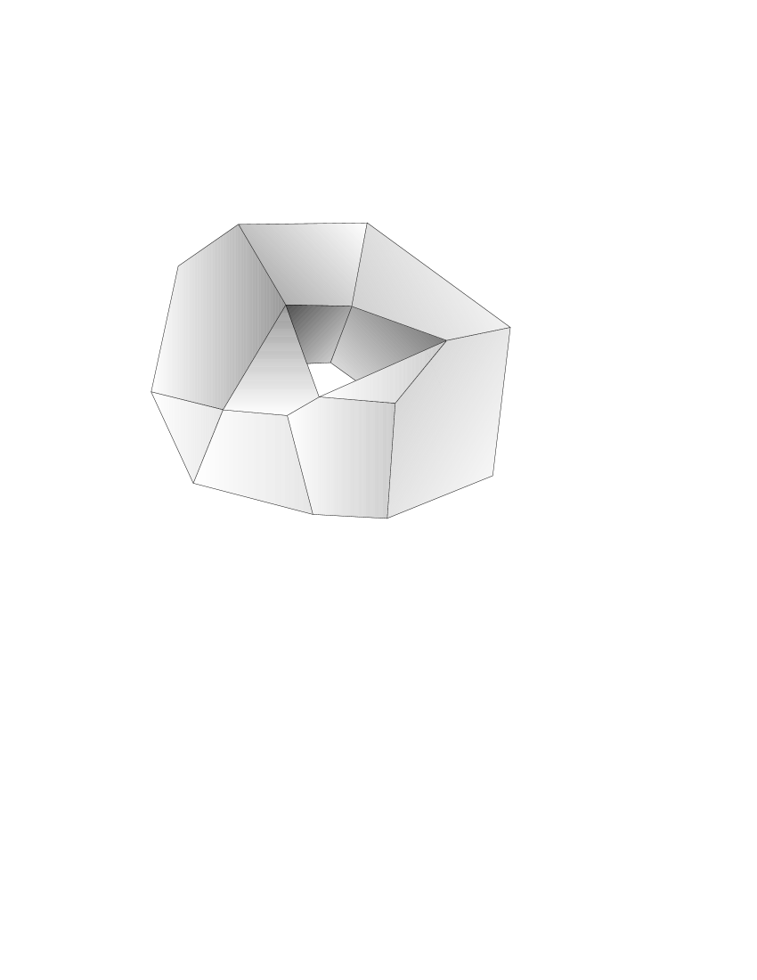
Figure 3: A cubist’s view of a discretized torus

This sum over surfaces can, in turn, be viewed as a Riemann sum for a certain vaguely defined “integral” over the infinite-dimensional space of all metrics on a genus $g$ surface. In 2-dimensional quantum gravity, one wants to integrate over this space of metrics; this is the reason why integrals (2.1) are studied there, see, in particular, [11, 20, 21, 31, 32] and [15, 16] for a survey.

More precisely, the relevant $N\to\infty$ asymptotic regime is when the number $n$ of pieces forming the surface grows, while the shapes $k_{i}$ of individual pieces remain bounded. For example, one can look at surfaces composed out of a large number of squares and hexagons. The corresponding (hard) mathematical problem is the $N\to\infty$ asymptotics of the integral

$$\int e^{-\frac{1}{2}\operatorname{tr}H^{2}+\operatorname{tr}P(H)}\,dH\,,$$ (2.2)

where $P(H)$ is a polynomial of $H$ the coefficients of which depend on $N$ in a certain critical fashion.

2.1.2 Witten’s conjecture

It was conjectured by Witten [93] that this discretized “integration” over the space of metrics is equivalent to certain topologically defined integrals over the (finite-dimensional) space of just the conformal classes of smooth metrics. Conformal, or, equivalently, complex structures on a genus $g$ surface form a finite-dimensional moduli space $\mathcal{M}_{g}$ of dimension $3g-3$ for $g>1$. The integrals in Witten’s conjecture are integrals of Chern classes of certain natural line bundles and, as a result, they have a topological interpretation as intersection numbers on a certain distinguished compactification $\overline{\mathcal{M}}_{g}\supset\mathcal{M}_{g}$.

This compactification $\overline{\mathcal{M}}_{g}$, constructed by Deligne and Mumford, is obtained by allowing nodal degenerations (of the kind seen on the left in Fig. 4) satisfying certain stability conditions, see, for example, [35]. Similarly, the moduli space $\mathcal{M}_{g,n}$ of smooth genus $g$ algebraic curves $C$ together with a choice of $n$-distinct marked points $p_{1},\dots,p_{n}\in C$ has a stable compactification $\overline{\mathcal{M}}_{g,n}$, which is a projective algebraic variety of dimension $3g-3+n$. For our purposes, it is somewhat more convenient to allow disconnected curves $C$. The disconnected and connected theories are, of course, equivalent.

By construction, a point of $\overline{\mathcal{M}}_{g,n}$ corresponds to an at worst nodal curve $C$ with a choice of $n$ smooth marked points $p_{i}\in C$. Since $p_{i}$ is a smooth point of $C$, one can consider the cotangent line $T^{*}_{p_{i}}C$ to $C$ at $p_{i}$. As the reference point in $\overline{\mathcal{M}}_{g,n}$ varies, these lines form a line bundle $\mathcal{L}_{i}$ over $\overline{\mathcal{M}}_{g,n}$. Consider the first Chern class of this bundle

$$c_{1}(\mathcal{L}_{i})\in H^{2}(\overline{\mathcal{M}}_{g,n})\,.$$

Witten’s conjecture (first proved in [52]) was that the natural generation function for the intersection numbers

$$\left\langle\tau_{k_{1}}\dots\tau_{k_{n}}\right\rangle=\int_{\overline{\mathcal{M}}_{g,n}}c_{1}(\mathcal{L}_{1})^{k_{1}}\dots c_{1}(\mathcal{L}_{n})^{k_{n}}\,,\quad\sum k_{i}=3g-3+n\,,$$ (2.3)

is precisely the $\tau$-function of the KdV hierarchy that emerged from the study of the matrix model of the 2D quantum gravity.

2.1.3 Edge of the spectrum and moduli of curves

The same $\tau$-function also arises in a mathematically much simpler asymptotic regime of the integral (2.1), namely the one in which the $k_{i}$’s go to infinity simultaneously with $N\to\infty$, while their number $n$ remains bounded. It is clear that the largest eigenvalues of $H$ dominate this asymptotics. Since the distribution of eigenvalues of $H$ near the edge of its spectrum is well known to converge to the Airy ensemble, this limit is very easy to control.

Somewhat surprisingly, it is this simpler matrix model that has a natural geometric relation to $\overline{\mathcal{M}}_{g,n}$, as discussed in detail in [72] and also, e.g., in [70], leading, in particular, to another, and in several respects more satisfying, proof of Witten’s conjecture.

2.2 Gromov-Witten theory of $\mathbb{P}^{1}$

One explanation of why the two very different asymptotic regimes lead to the same result is the following. The intersection theory of $\overline{\mathcal{M}}_{g,n}$ embeds, in fact in many different ways, into a certain richer geometric theory which, as it turns out, can be described by the Plancherel measure analog of (2.1) on a finite level, that is, without taking any limits.

2.2.1 Stable maps and GW invariants

This richer theory is the Gromov-Witten theory of the Riemann sphere $\mathbb{P}^{1}$, which is defined using intersection theory on the moduli space $\overline{\mathcal{M}}_{g,n}(\mathbb{P}^{1},d)$ of stable maps to $\mathbb{P}^{1}$, see e.g. [28]. By definition, a point in the space of stable maps is described by the data

$$f:(C,p_{1},\dots,p_{n})\to\mathbb{P}^{1}\,,$$ (2.4)

where $f$ is a degree $d$ holomorphic map whose domain $C$ is a possibly nodal curve of genus $g$ with smooth marked points $p_{i}\in C$, see Figure 4.

Figure 4: A schematic view of a boundary element in $\overline{\mathcal{M}}_{3,5}(\mathbb{P}^{1})$

Here, again, possible degenerations of the domain $C$ are limited by a certain stability condition.

An open (but not dense) subset

$$\mathcal{M}_{g,n}(\mathbb{P}^{1},d)\subset\overline{\mathcal{M}}_{g,n}(\mathbb{P}^{1},d)$$

is formed by maps with smooth domains $C$. In this case $f$ represents $C$ as a Riemann surface of an algebraic function of degree $d$. Generically, $f$ has only nondegenerate critical points, the number of which equals $2d+2g-2$ by Riemann-Hurwitz. The corresponding critical values together with the $n$ images $f(p_{i})\in\mathbb{P}^{1}$ of the marked points give convenient local coordinates on a neighborhood of such map $f$. The number $2d+2g-2+n$ is known as the (complex) expected dimension of $\overline{\mathcal{M}}_{g,n}(\mathbb{P}^{1},d)$.

The whole $\overline{\mathcal{M}}_{g,n}(\mathbb{P}^{1},d)$ is not so nice, being reducible with components of different dimensions. One defines, however, a distinguished homology class

$$\left[\overline{\mathcal{M}}_{g,n}(\mathbb{P}^{1},d)\right]^{\textup{vir}}\in H_{*}(\overline{\mathcal{M}}_{g,n}(\mathbb{P}^{1},d))$$ (2.5)

of the expected dimension, known as the virtual fundamental class. Integration against (2.5) replaces in Gromov-Witten theory integration over fundamental class in (2.3).

The most fundamental part of the Gromov-Witten theory of $\mathbb{P}^{1}$ is its stationary sector, obtained by pinning down the images of the marked points by requiring $f(p_{i})=q_{i}$, where $q_{i}\in\mathbb{P}^{1}$ are arbitrary distinct points. The stationary GW invariants of $\mathbb{P}^{1}$ are, by definition, the following numbers

$$\left\langle\tau_{k_{1}}(\textup{pt})\,\dots\,\tau_{k_{n}}(\textup{pt})\right\rangle_{d}=\int_{\left[\overline{\mathcal{M}}_{g,n}(\mathbb{P}^{1},d)\right]^{\textup{vir}}\bigcap\{f(p_{i})=q_{i}\}_{i=1\dots n}}c_{1}(\mathcal{L}_{1})^{k_{1}}\dots c_{1}(\mathcal{L}_{n})^{k_{n}}\,,$$ (2.6)

where the classes $c_{1}(\mathcal{L}_{i})$ are defined as before. Note that the genus $g$ is uniquely determined by the dimension constraint

$$\sum k_{i}=2d+2g-2$$

and, therefore, is omitted in the left-hand side of (2.6).

2.2.2 Plancherel measure and GW invariants of $\mathbb{P}^{1}$

In order to write down the Plancherel measure analog of the matrix integral (2.1) we need the partition analog of the function

$$\operatorname{tr}H^{k}=\sum_{i=1}^{N}x_{i}^{k}\,.$$ (2.7)

It is given by the following function

$$\mathbf{p}_{k}(\lambda) =\sum_{i}\left[\left(\lambda_{i}-i+\tfrac{1}{2}\right)^{k}-\left(-i+\tfrac{1}{2}\right)^{k}\right]+\left(1-2^{-k}\right)\,\zeta(-k)$$ (2.8)

$$\textup{\!``=''}\sum_{x\in\mathfrak{S}(\lambda)}x^{k}\,,$$

where the first line the $\zeta$-regularization of the direct, but divergent, generalization of (2.7) written in second line. Equivalently,

$$\frac{1}{z}+\sum_{k}\mathbf{p}_{k}(\lambda)\,z^{k}=\sum_{i}e^{z(\lambda_{i}-i+\frac{1}{2})}=(\mathcal{E}(z)\cdot v_{\lambda},v_{\lambda})\,,$$ (2.9)

where $\mathcal{E}(z)$ is the following diagonal matrix in $\mathfrak{gl}(V)$

$$\mathcal{E}(z)\cdot e_{k}=e^{zk}\,e_{k}\,.$$ (2.10)

We now ready to state the following result from [73]

Theorem 1

$$\left\langle\tau_{k_{1}}(\textup{pt})\,\dots\,\tau_{k_{n}}(\textup{pt})\right\rangle_{d}=\frac{1}{\prod(k_{i}+1)!}\,\sum_{|\lambda|=d}\left(\frac{\dim\lambda}{d!}\right)^{2}\,\prod\mathbf{p}_{k_{i}+1}(\lambda)\,.$$ (2.11)

As explained above, the right-hand side of (2.11) is a direct analog of the integral (2.1) for partitions of finite size $d$, where $d$ is the degree of GW invariant on the left. In particular, this formula is highly nontrivial already for $d=0$, reproducing a result of [27]. There is only one partition of $0$, namely the empty partition $\emptyset$ and $\mathbf{p}_{k}(\emptyset)$ equals the $\zeta$-term in (2.8), illustrating the naturality of the $\zeta$-regularization.

Theorem 1 continues to hold for stationary GW invariants of any smooth curve $X$, with the following modification:

$$\left(\frac{\dim\lambda}{d!}\right)^{2}\mapsto\,\left(\frac{\dim\lambda}{d!}\right)^{2-2g(X)}\,,$$

where $g(X)$ is the genus of $X$. In particular, genus 1 targets lead to the uniform measure on partitions.

2.2.3 Operator form of the GW theory

We reproduced here the formula (2.11) to emphasize the role of the Plancherel measure in the GW theory. It is, however, very much not the final answer in the theory. Using (2.9) and (1.8), one rewrites (2.11) as follows

$$\sum_{k_{i}}\left\langle\prod\tau_{k_{i}}(\textup{pt})\right\rangle_{d}\prod z_{i}^{k_{i}+1}=\frac{1}{(d!)^{2}}\left\langle\alpha_{1}^{d}\,\prod\mathcal{E}(z_{i})\,\alpha_{-1}^{d}\right\rangle\,,$$ (2.12)

where the angle brackets on the right denote the vacuum expectation

$$\left\langle M\right\rangle=(Mv_{\emptyset},v_{\emptyset})\,,$$

of an operator $M$ acting on ${\bigwedge}^{\!\frac{\infty}{2}}V$.

Using the commutation relations between the operators $\alpha_{n}$ and $\mathcal{E}(z)$, one evaluates (2.12) in closed form in terms of trigonometric functions [73]. For example, the $1$-point function has an especially simple form

$$\sum_{g\geq 0}\left\langle\tau_{2g-2+2d}(\textup{pt})\right\rangle^{\circ}_{d}\,z^{2g}=\frac{1}{(d!)^{2}}\,\mathcal{S}(z)^{2d-1}\,,\quad\mathcal{S}(z)=\frac{\sinh z/2}{z/2}\,,$$ (2.13)

where the superscript ^∘ denotes the connected GW invariant.

In the case when the target $X$ is an elliptic curve $E$, the vacuum matrix element is replaced by trace

$$\sum_{d\geq 0}q^{d}\sum_{k_{i}}\left\langle\prod\tau_{k_{i}}(\textup{pt})\right\rangle_{d}^{E}\prod z_{i}^{k_{i}+1}=\operatorname{tr}_{0}q^{L_{0}}\prod\mathcal{E}(z_{i})\,,$$ (2.14)

where $L_{0}$ is the energy operator defined by

$$L_{0}\cdot v_{\lambda}=|\lambda|\,v_{\lambda}\,,$$

and $\operatorname{tr}_{0}$ denotes the trace in the zero charge subspace (spanned by the vectors $v_{\lambda}$). The sum (2.14) was computed in [7] in terms of genus 1 theta functions with modular parameter $q$, see also [69].

From the operator interpretation, one derives Toda equations. These equations were conjectured in [22, 23], see also [29, 30, 76], and translate into effective recurrence relations for the GW invariants of $\mathbb{P}^{1}$. The integrable structure of the GW theory fully unfolds in the equivariant GW theory of $\mathbb{P}^{1}$, which is described by the 2-dimensional Toda hierarchy of Ueno and Takasaki [88]. The 2D Toda hierarchy is derived from the operator solution of the theory in [74]. The description of the nonstationary sector of the theory is completed in [75].

3 More random partitions from geometry

3.1 Hurwitz theory

The Gromov-Witten theory of target curves is closely related to the much older and much more elementary Hurwitz theory [36] that concerns enumeration of degree $d$ branched covers

$$f:C\to X$$

of a smooth curve $X$ with specified ramifications. What this means is: we require $f$ to be unramified outside some fixed set of points $\{q_{i}\}\in X$ and for each point $q_{i}$ we specify the conjugacy class in the symmetric group $S(d)$ of the monodromy of the branched cover $f$ around $q_{i}$. In other words, for every $q_{i}$ we specify a partition $\eta^{(i)}$ of the number $d$.

By cutting the base $X\setminus\{q_{i}\}$ (and hence the cover $C$) into simply-connected pieces, one can see many connections between the Hurwitz theory and enumeration of maps on $C$ discussed in Section 2.1.1.

A classical formula of Burnside [13, 41] tells us that the number of such covers, automorphism-weighted and possibly disconnected, equals

$$\sum_{|\lambda|=d}\left(\frac{\dim\lambda}{d!}\right)^{2-2g(X)}\,\prod\mathbf{f}_{\eta^{(i)}}(\lambda)\,,$$ (3.1)

where $g(X)$ is the genus of $X$ and $\mathbf{f}_{\eta}(\lambda)$ is the central character of the representation $\lambda$, that is, the unique eigenvalue of the matrix by which the conjugacy class $\eta$ acts in the irreducible representation $\lambda$.

By a theorem of Kerov and Olshanski [51]

$$\mathbf{f}_{\eta}\in\Lambda^{*}=\mathbb{Q}[\mathbf{p}_{1},\mathbf{p}_{2},\mathbf{p}_{3},\dots]\,,$$ (3.2)

which shows that from the random partitions point of view there is no real difference between (2.11) and (3.1). This is a manifestation of the Gromov-Witten/Hurwitz correspondence, established in [73].

3.2 Uniform measure and ergodic theory

Note from (3.1) that enumeration of degree $d$ branched covering of the torus is related to the uniform measure on partitions of $d$. The large $d$ asymptotics in this problem is interesting, because, on the geometric side, it computes the volumes of moduli spaces of pairs $(C,\omega)$ where $C$ is a smooth curve and $\omega$ a holomorphic differential on $C$ with given multiplicities of zeros [26]. This is because points of the form $(C,f^{*}(dz))$, where

$$f:C\to\mathbb{C}\big{/}\mathbb{Z}^{2}$$

is a branched covering of a standard torus, play the role of lattice points in this moduli space.

The moduli spaces of holomorphic differentials and, in particular, their volumes are important in ergodic theory, for example, for the study of billiards in rational polygons [25]. The exact evaluation of the sum (2.14) and the modular properties of the answer were of great help for the asymptotic analysis performed in [26]. The modular transformation exchanges the $q\to 1$ limit with the $q\to 0$ limit in (2.14), which means relating large partitions to small partitions. This is an example of a mirror phenomenon, see for example the discussion in [18].

3.3 Random partitions from localization

A constant source of partition sums in geometry is equivariant localization [2]. Partitions index fixed points of the torus action on the Grassmann varieties (in the Plücker embedding, these are precisely the vectors $v_{\lambda}$). They also index fixed points of the torus action on $\operatorname{Hilb}_{n}(\mathbb{C}^{2})$, the Hilbert scheme of $n$ points in the plane $\mathbb{C}^{2}$, see e.g. [33, 63].

3.3.1 Hilbert scheme of points in the plane

By definition, a point in $\operatorname{Hilb}_{n}(\mathbb{C}^{2})$ is an ideal $I\in\mathbb{C}[x,y]$ of codimension $n$ as a linear subspace, such as, for example, the space of polynomials vanishing at $n$ given distinct points in the plane. The torus $(\mathbb{C}^{\times})^{2}$ acts on $\operatorname{Hilb}_{n}(\mathbb{C}^{2})$ by dilating the coordinates $x$ and $y$. Its fixed points are the monomial ideals, that is, ideals spanned by monomials $x^{i}y^{j}$. Monomial ideals $I$ are naturally indexed by partitions of $n$, namely, the set $\{(i,j),\,x^{i}y^{j}\notin I\}$ is, essentially, a diagram of a partition.

In equivariant localization, the contribution of an isolated fixed point $I$ appears with a weight which the reciprocal of the product of the weights of the torus action on the tangent space $T_{I}$ at $I$. Let $\epsilon_{1}$ and $-\epsilon_{2}$ be the weights of the torus action on $\mathbb{C}[x,y]$. Then, up to a sign, the natural measure on partitions that arises is the following Jack polynomials deformation $\mathfrak{M}_{\textup{Jack}}$ of the Plancherel measure.

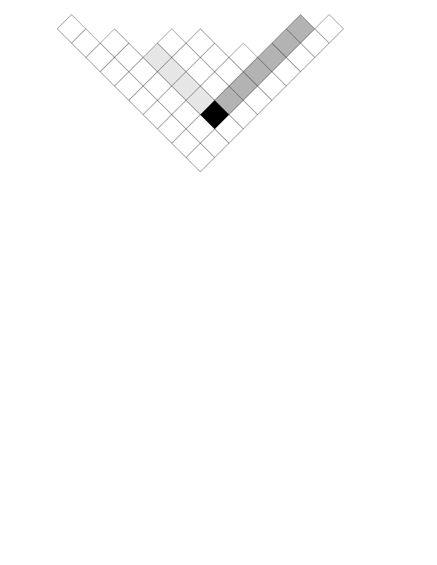
Figure 5: The hook, arm, and leg of a square

3.3.2 Jack deformation of the Plancherel measure

Recall the hook-length formula

$$\frac{\dim\lambda}{|\lambda|!}=\prod_{\square\in\lambda}h(\square)^{-1}\,,$$ (3.3)

where the product is over all squares $\square$ in the diagram of $\lambda$ and $h(\square)$ is the length of the hook of the square $\square$, see Fig. 5.

We have $h(\square)=1+a(\square)+l(\square)$, where $a(\square)$ and $l(\square)$ are the arm- and leg-length of $\square$, indicated by different shades of gray in Fig. 5. In the deformed measure $\mathfrak{M}_{\textup{Jack}}$ one takes arm- and leg-length with different weights. Concretely, one sets

$$\mathfrak{M}_{\textup{Jack}}(\lambda)=\prod_{\square\in\lambda}\frac{1}{\Big{(}(1+a(\square))\epsilon_{1}+l(\square)\epsilon_{2}\Big{)}\Big{(}a(\square)\epsilon_{1}+(1+l(\square))\epsilon_{2}\Big{)}}\,.$$ (3.4)

Up to an overall factor, $\mathfrak{M}_{\textup{Jack}}$ clearly depends only on the ratio $\epsilon_{1}/\epsilon_{2}$. To make $\mathfrak{M}_{\textup{Jack}}$ a probability measure on partitions of $d$, one has to multiply it by $d!\,(\epsilon_{1}\epsilon_{2})^{d}$.

The measure $\mathfrak{M}_{\textup{Jack}}$ should be viewed as the general $\beta$ analog of the Plancherel measure with $\beta=2\epsilon_{1}/\epsilon_{2}$. Recall that in random matrix theory by ensembles with general $\beta$ one means the generalization of the measure (1.5) in which Vandermonde squared is replaced by $\prod|x_{i}-x_{j}|^{\beta}$. Like in the random matrix theory, the measure $\mathfrak{M}_{\textup{Jack}}$ shares some features of Plancherel measure and lacks others. Most importantly, the free fermion interpretation is lacking, making, for example, the computation of the correlation functions of $\mathfrak{M}_{\textup{Jack}}$ a difficult open problem.

We will see this measure again in Section 5. Also note that the symmetry $\beta\mapsto 4/\beta$, of which there are some instances in the random matrix theory, is manifest for the discrete measure $\mathfrak{M}_{\textup{Jack}}$.

4 Schur measure

4.1 Definition and correlation functions

4.1.1 Schur functions

A generalization of the Plancherel measure, which in many ways resembles placing a random matrix into an arbitrary potential, is defined as follows. Let $t_{1},t_{2},\dots$ be parameters. The polynomials

$$s_{\lambda}(t)=\left(\exp\left(\sum_{n>0}t_{n}\,\alpha_{-n}\right)\cdot v_{\emptyset},v_{\lambda}\right)\,,$$

indexed by partitions $\lambda$, are known as the Schur functions. Upon the substitution

$$t_{k}=\frac{1}{k}\operatorname{tr}H^{k}\,,$$

the polynomial $s_{\lambda}$ becomes the trace of a matrix $H\in GL(n)$ in the irreducible representation of $GL(n)$ with highest weight $\lambda$.

As a generalization of (1.8), we introduce the Schur measure on partitions by the following formula

$$\mathfrak{M}_{\textup{Schur}}(\lambda)=\frac{1}{\mathcal{Z}}\,s_{\lambda}(t)\,s_{\lambda}(\bar{t})\,.$$ (4.1)

Here $t$ and $\bar{t}$ are two independent sets of variables. Choosing one set to be the complex conjugate of the other is sufficient to guarantee that $\mathfrak{M}_{\textup{Schur}}(\lambda)\geq 0$. This positivity, however, is largely irrelevant for what follows. The normalizing factor $\mathcal{Z}$ in (4.1) is given by the Cauchy identity

$$\mathcal{Z}=\sum_{\lambda}s_{\lambda}(t)\,s_{\lambda}(\bar{t})=\exp\left(\sum_{k}k\,t_{k}\bar{t}_{k}\right)\,.$$ (4.2)

Applying the operator $\sum_{k>0}t_{k}\partial_{t_{k}}$ to (4.2) we see that the expected size $\left\langle|\lambda|\right\rangle$ of $\lambda$ with respect to the Schur measure equals

$$\left\langle|\lambda|\right\rangle=\sum_{k}k^{2}t_{k}\bar{t}_{k}\,.$$

4.1.2 Schur measure and relative GW theory

Schur measure naturally arises, for example, in the relative Gromov-Witten theory of $\mathbb{C}^{\times}=\mathbb{P}^{1}\setminus\{0,\infty\}$, see [73]. This relative Gromov-Witten theory is certain hybrid of GW and Hurwitz theory, in which one insist that the map $f:C\to\mathbb{P}^{1}$ has given ramification over $0,\infty\in\mathbb{P}^{1}$ (but what precisely having given ramifications means when $C$ is not smooth is too technical to describe here). Informally, these two ramifications can be thought as in- and out-going states of an interaction described by the “worldsheet” $C$. The variables $t$ and $\bar{t}$ are the generating function variables coupled to the cycles of the in- and out-going ramifications.

4.1.3 Correlation functions of the Schur measure

A remarkable property of the Schur measures is that it is possible to compute their correlations in closed form. Like for random matrices, the $n$-point correlations are given by $n\times n$ determinants with a certain correlation kernel $\mathsf{K}$. Unlike random matrices, the kernel $\mathsf{K}$ does not involve any delicate objects like polynomials orthogonal with an arbitrary weight [14, 59]. On the contrary, the kernel $\mathsf{K}$ has a simple integral representation in terms of the parameters $t$ and $\bar{t}$, which is particularly suited for the steepest descent asymptotic analysis.

Introduce the function $T(z)$ by

$$T(z)=\sum_{k>0}t_{n}\,z^{n}-\sum_{k>0}\bar{t}_{n}\,z^{-n}\,.$$

Let us assume that it converges in some neighborhood of the unit circle (the case when $T(z)$ is a polynomial is already interesting enough). The correlation function of the Schur measure were computed in [69] in the following form

Theorem 2

For any $X\subset\mathbb{Z}+\frac{1}{2}$ we have

$$\operatorname{Prob}_{\,\mathfrak{M}_{\textup{Schur}}}\big{\{}X\subset\mathfrak{S}(\lambda)\big{\}}=\det\big{[}\mathsf{K}(x_{i},x_{j})\big{]}_{x_{i},x_{j}\in X}\,,$$ (4.3)

where the kernel $\mathsf{K}$ is given by

$$\mathsf{K}(x,y)=\frac{1}{(2\pi i)^{2}}\iint_{|w|<|z|}\frac{e^{T(z)-T(w)}}{z-w}\,\frac{dzdw}{z^{x+\frac{1}{2}}{w^{-y+\frac{1}{2}}}}\,.$$ (4.4)

The proof of this formula uses the algebra of the infinite wedge representation ${\bigwedge}^{\!\frac{\infty}{2}}V$. In the same spirit, one shows that the for any fixed set $X$ the sequence correlation functions

$$\tau^{X}_{n}(t,\bar{t})=\operatorname{Prob}\big{\{}X+n\subset\mathfrak{S}(\lambda)\big{\}}\,,$$

where $X+n$ denotes the translation of the set $X$ by $n$ lattice spacings, is a sequence of $\tau$-function for the Ueno–Takasaki 2-dimensional Toda hierarchy with respect to the two sets of (higher) times $t$ and $\bar{t}$.

4.2 Asymptotics and limit shapes

4.2.1 Asymptotics of the correlation functions

Our goal now is to explain how convenient is the representation (4.4) for the steepest descent analysis. For simplicity, let us assume that the variables $\bar{t}$ are complex conjugate of $t$. The interesting asymptotic regime is when all variables $t$ grow at the same rate, that is, when $T(z)=MP(z)$, where $M\to\infty$ and $P(z)$ is fixed. As we will see, this implies that the typical partition is of length $O(M)$ in both directions, and hence contains $O(M^{2})$ squares. We will investigate $\mathsf{K}(x_{1},x_{2})$ in this limit assuming that

$$\frac{x_{i}}{M}\to\bar{x}\,,\quad x_{1}-x_{2}\to\Delta x\,.$$ (4.5)

The number $\bar{x}$ describes our global position on the limit shape; the number $\Delta x$ is the relative local displacement.

The exponentially large term in the integral (4.4) is $e^{M(S(z)-S(w))}$, where

$$S(z)=P(z)-\bar{x}\,\log z\,.$$ (4.6)

By our hypothesis, $S(z)$ is purely imaginary on the unit circle $|z|=1$ and hence the integrand is rapidly oscillating there. We want to shift the contour of integration in $z$ (resp. $w$) off the unit circle in the direction of $\mp\operatorname{grad}\Re S$, so that to make the integrand exponentially small. This direction is given by the sign of

$$g(\phi)-\bar{x}\,,\quad\textup{where}\quad g(\phi)=\left.z\frac{d}{dz}P(z)\right|_{z=e^{i\phi}}\,.$$ (4.7)

The function $g$ is a real-valued analytic function on the circle, and the set of points where $g\geq\bar{x}$ is a finite union of intervals

$$\{\phi,g(\phi)\geq\bar{x}\}=\bigsqcup_{i}[\alpha_{i}(\bar{x}),\beta_{i}(\bar{x})]\,,$$ (4.8)

see Fig. 6.

Figure 6: Construction of the intervals $[\alpha_{i}(\bar{x}),\beta_{i}(\bar{x})]$

The set (4.8) varies from whole circle to the empty set as $\bar{x}$ varies from the minimal to the maximal value of the function $g$. These extreme values mark the edges of the limit shape.

The integration in (4.4) is along two nested circles. When we deform the $z$ and $w$ contours in the direction of $\mp g(\phi)$ as in Fig. 7, we pick up the residue of the integrand at $z=w$ whenever we push the $z$-contour inside the the $w$-contour.

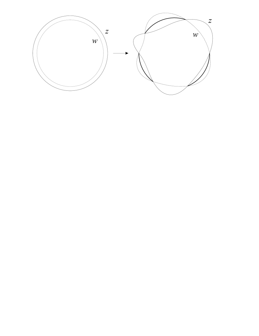
Figure 7: Deformation of the integration contours

At $z=w$, most of the factors in the integrand cancel out, so we are left with

$$\frac{1}{(2\pi i)^{2}}\iint_{|w|<|z|}(\dots)=\frac{1}{(2\pi i)^{2}}\iint_{\textup{deformed contour}}(\dots)+\frac{1}{2\pi}\sum_{i}\int_{\alpha_{i}(\bar{x})}^{\beta_{i}(\bar{x})}\frac{d\phi}{e^{\phi\Delta x}}\,.$$ (4.9)

By the basics of the steepest descent method, the first summand in the right-hand side of (4.9) goes to $0$ as $M\to\infty$. We obtain

Theorem 3

As $M\to\infty$, we have

$$\mathsf{K}(x_{1},x_{2})\to\frac{\sum_{i}\left(e^{-\alpha_{i}(\bar{x})\,\Delta x}-e^{-\beta_{i}(\bar{x})\,\Delta x}\right)}{2\pi\Delta x}\,.$$ (4.10)

Note that (4.10) is a multi-frequency generalization of the discrete sine kernel (4.13). In particular, the 1-point function, which determines the density of particles and, hence, the limit shape, satisfies

$$\operatorname{Prob}\big{\{}x\in\mathfrak{S}(\lambda)\big{\}}=K(x,x)\to\frac{\sum_{i}|\beta_{i}(\bar{x})-\alpha_{i}(\bar{x})|}{2\pi}\,.$$ (4.11)

This density decreases from $1$ to $0$ as $\bar{x}$ varies in $[\min g,\max g]$ and, hence, these numbers indeed mark the boundary of the limit shape.

Note that the the density (4.11) is monotone and hence the limit shape is always convex. Also note that the random process defined by the correlation kernel (4.10) is translation invariant.

4.2.2 Example: Plancherel measure

The Schur measure specializes to the measure $\mathfrak{M}_{\textup{PP}}$ when

$$t,\bar{t}=\left(\sqrt{\xi},0,0,\dots\right)\,.$$

Plugging this into (4.4) leads to the discrete Bessel kernel defined by

$$\mathsf{K}_{\textup{Bessel}}(x,y;\xi) =\frac{1}{(2\pi i)^{2}}\iint_{|w|<|z|}\frac{e^{\sqrt{\xi}(z-z^{-1}-w+w^{-1})}}{z-w}\,\frac{dz\,dw}{z^{x+\frac{1}{2}}\,w^{-y+\frac{1}{2}}}$$

$$=\sqrt{\xi}\,\,\frac{J_{x-\frac{1}{2}}\,J_{y+\frac{1}{2}}-J_{x+\frac{1}{2}}\,J_{y-\frac{1}{2}}}{x-y}\,,$$ (4.12)

where $J_{n}=J_{n}(2\sqrt{\xi})$ is the Bessel function of order $n$. This formula is a limit case of the main result of [10]. It appears as stated in [8] and [39].

We have $M=\sqrt{\xi}$ and $g(\phi)=2\cos(\phi)$. Therefore,

$$\beta_{1}(\bar{x})=-\alpha_{1}(\bar{x})=\arccos\left(\bar{x}\big{/}2\right)\,.$$

Integrating the density $\frac{1}{\pi}\arccos\frac{\bar{x}}{2}$, one arrives at the at the limit shape for the Plancherel measure first obtained by Vershik and Kerov [90] and Logan and Shepp [54]. In the bulk $\bar{x}\in(-2,2)$ of this limit shape, we have the (unscaled) convergence of $\mathfrak{S}(\lambda)$ to the discrete sine-kernel ensemble with the correlation kernel

$$\mathsf{K}_{\textup{sin}}(x,y;a)=\frac{\sin a(x-y)}{\pi(x-y)}\,,\quad a=\arccos\left(\bar{x}\big{/}2\right)\,.$$ (4.13)

In the continuous situation, the parameter $a$ in (4.13) can be scaled away, but on a lattice it remains a nontrivial parameter. In fact, a finer analysis performed in [8] shows that the we have the same convergence to the discrete sine kernel for the Plancherel measure partitions of fixed size $n$ as $n\to\infty$.

Near the edge of limit shape, the random process $\mathfrak{S}(\lambda)$ converges, after a suitable scaling to the Airy ensemble. In our setup, this can be seen by analyzing the previously discarded first summand in the right-hand side of (4.9). On the edge of the limit shape, $\bar{x}$ is a critical value of $g$ and, hence, the corresponding critical point of the action (4.6) is degenerate. The Airy kernel appears effortlessly in the asymptotics (see, for example, [71] for a pedagogical exposition).

The depoissonization analysis performed in [8] and [39] shows that the same Airy ensemble asymptotics remains valid for Plancherel measure on partition of fixed size $n$ as $n\to\infty$. This is precisely the statement of a conjecture of Baik, Deift, and Johansson, first established in [68] by different means.

5 Random partitions in Seiberg-Witten theory

5.1 Gauge theory partition function

5.1.1 Plancherel measure in a periodic potential

Fix a period $N$ and let $u_{\frac{1}{2}},u_{\frac{3}{2}},\dots,u_{N-\frac{1}{2}}$ be such that $\sum u_{k}=0$. Consider the period $N$ periodic potential $U$ on the lattice $\mathbb{Z}+\frac{1}{2}$ defined by $U(x)=u_{x\operatorname{mod}N}$. Define the energy of the particle configuration $\mathfrak{S}(\lambda)$ in the potential $U$ by

$$U(\lambda)=\sum_{\begin{subarray}{c}x\in\mathfrak{S}(\lambda),\,\,x>-MN\end{subarray}}u(x)\,.$$ (5.1)

This does not depend on the cut-off $M$ as long as $M$ is a sufficiently large integer.

We now define the (poissonized) Plancherel measure in the periodic potential $U$ by

$$\mathfrak{M}_{U}(\lambda)=\xi^{|\lambda|}\,\exp\left(\frac{1}{\hbar}\,U(\lambda)\right)\,\left(\frac{\dim\lambda}{|\lambda|!}\right)^{2}\,.$$ (5.2)

The properties of this measure are in many ways parallel to the theory of periodically weighted planar dimers, developed in [44].

5.1.2 Instantons and Seiberg-Witten prepotential

In (5.2), we dropped the normalization factor $e^{-\xi}$ present in (1.3) because the understanding of the partition function for $\mathfrak{M}_{U}$ is, anyway, the main problem in the theory. This is because this partition function, as shown in Section 5 of [67], is essentially the Fourier transform of the $\mathcal{N}=2$ pure supersymmetric $SU(N)$-gauge theory partition functions, as computed by Nekrasov in [65] via instanton calculus.

For mathematicians, this gauge theory partition function is a generating function for certain integrals over the moduli spaces of instantons. These are topologically defined finite-dimensional integrals, so there is a certain similarity in spirit with Witten’s formulation of the 2D quantum gravity, discussed in Section 2.1.2. The actual geometry of the instanton moduli spaces seems somewhat more accessible than the geometry of $\overline{\mathcal{M}}_{g,n}$. The equivariant localization approach to these instanton integrals, initiated in [56, 57] and completed in [65], is a far reaching generalization of what we saw in Section 3.3. In particular, partition sums appear as sums over fixed points.

The main expected feature of this partition function is that its quasiclassical

$$\xi\to\infty\,,\quad\hbar\to 0\,,$$

asymptotics should be described by the Seiberg-Witten prepotential [82, 83]. This was indeed demonstrated in [67] and this is where the large random partitions come in. I refer to [66] for more on the geometrical and physical side of this computation; here we will focus on purely the random partition aspect of it. An introduction to the Seiberg-Witten theory for a mathematical audience can be found in [19]. It also contains many further references. A different, non-asymptotic, approach to the analysis of the partition function can be found in [64].

The case of the pure gauge theory is just the beginning of the Seiberg-Witten theory. Various theories with matter lead to related measures on partitions. They are also considered in [67].

5.2 Asymptotics

5.2.1 Quasiclassical scaling and measure concentration

Let $\xi$ be very large. Then ${\xi^{|\lambda|}}\big{/}{|\lambda|!}$ has a sharp peak around $|\lambda|\approx\xi$. For $|\lambda|\approx\xi$, the weight $\dim\lambda$ can be approximately computed as follows. Let $f$ be the profile $f_{\lambda}(x)$ scaled in both directions by $\sqrt{|\lambda|}$, so that to make the area of the scaled diagram equal to $1$. By the results of [54, 90, 92]

$$\log\,\xi^{|\lambda|}\,\left(\frac{\dim\lambda}{|\lambda|!}\right)^{2}\sim-|\lambda|\,E(f)\,,$$ (5.3)

where the functional $E(f)$ is defined by

$$E(f)=2\iint_{s<t}(1+f^{\prime}(s))(1-f^{\prime}(t))\log 2(t-s)\,ds\,dt\,.$$ (5.4)

A direct argument shows that, with the same scaling,

$$\frac{1}{\hbar}\,U(\lambda)\sim\frac{\sqrt{|\lambda|}}{2\hbar}\,\int\sigma_{U}(f^{\prime}(t))\,dt\,,$$ (5.5)

where $\sigma_{U}(x)$ is a convex continuous function on $[-1,1]$, which is linear on the segments $\big{[}-1+\frac{2i}{N},-1+\frac{2(i+1)}{N}\big{]}$, $i=0,\dots,N-1$, such that the set $\{u_{k}\}$, sorted in the decreasing order, is the set of slopes of $\sigma_{U}$. The function $\sigma_{U}$ has the meaning of surface tension. An example of $\sigma_{U}$ can be seen in Fig. 8.

Figure 8: The surface tension for $\{u_{k}\}=\{4,1,-2,-3\}$

Note that the surface tension $\sigma_{U}$ is invariant under permutations of the $u_{i}$’s, so in what follows we will assume that

$$u_{\frac{1}{2}}>u_{\frac{3}{2}}>\dots>u_{N-\frac{1}{2}}\,.$$

We see that (5.3) and (5.5) have the same scale when

$$\xi\sim\operatorname{const}\,\hbar^{-2}\sim|\lambda|\,.$$

In this asymptotic regime, the measure $\mathfrak{M}_{U}$ concentrates on the maximizer of the functional

$$S(f)=-E(f)+\operatorname{const}\int\sigma_{U}(f^{\prime}(t))\,dt\,.$$ (5.6)

This functional is strictly concave and has a unique global maximizer $f^{\star}$. By construction, the value $S(f^{\star})$ of the functional (5.6) at its maximizer $f^{\star}$ dominates the partition function and hence we expect to identify it with the Seiberg-Witten prepotential.

Note that the surface tension $\sigma_{U}(x)$ is not differentiable at the points $x=-1+\frac{2i}{N}$. In crystallography, such singularities are often called cusps. From general principles, one expects that the cusps of $\sigma_{U}(x)$ result in facets of the maximizer $f^{\star}$, that is, the limit shape $f^{\star}$ develops straight-line pieces with slopes in the set $\left\{-1+\frac{2i}{N}\right\}$.

5.2.2 Construction of the minimizer

The construction of the maximizer $f^{\star}$ is the following. Let $\Delta$ be the half-strip $|\Re w|<1$, $\Im w>0$ in the complex plane with vertical slits going up from the points $-1+\frac{2i}{N}$, $i=1,\dots,N-1$, see Fig. 9. The lengths of the slits will be fixed later.

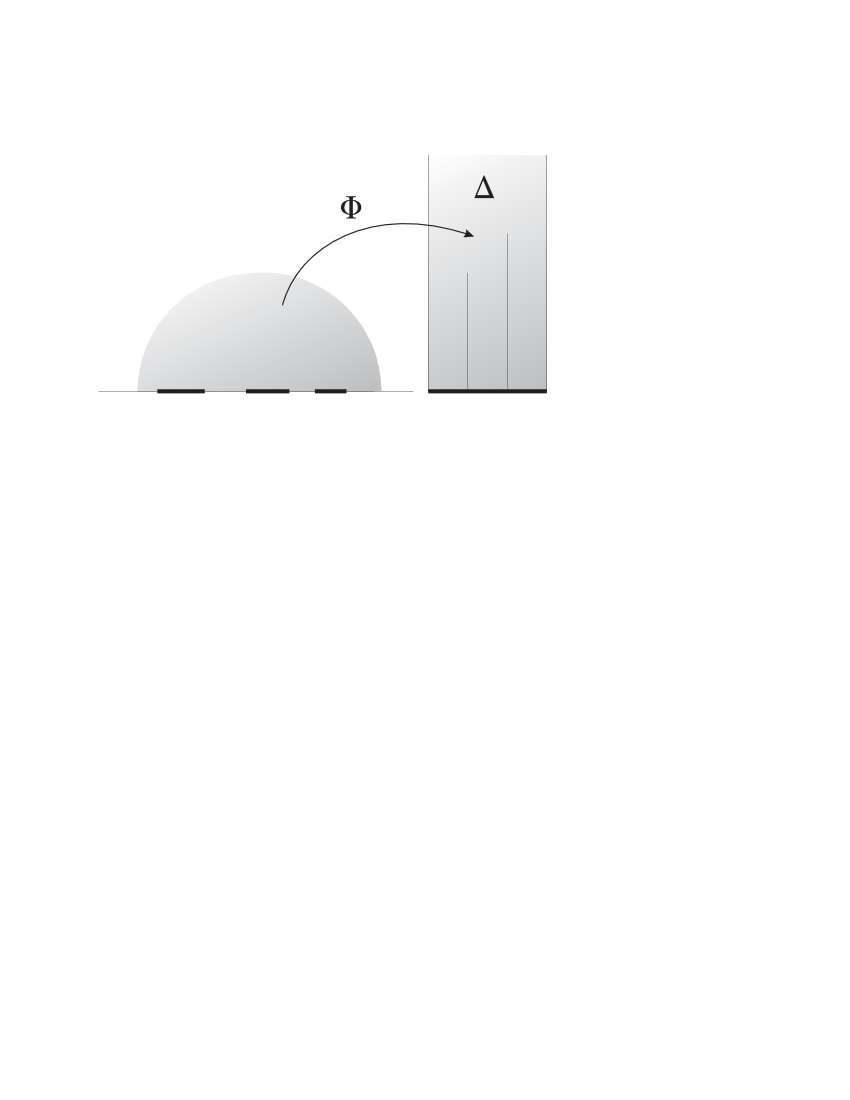
Figure 9: The conformal map used in the construction of the maximizer (here $N=3$)

Let $\Phi$ be the conformal map from the upper half-plane to the domain $\Delta$, sending infinity to infinity. The map $\Phi$ has a certain natural normalization at infinity, which fixes it uniquely.

Note that $\mathbb{R}$ naturally decomposes into segments of two kinds: those (called bands) mapped by $\Phi$ to the horizontal parts of $\partial\Delta$, and those (called gaps) mapped to the vertical parts of $\partial\Delta$. The slit-lengths of $\Delta$ are found from the $u_{i}$’s by fixing certain period of the differential

$$dS=z\,d\Phi(z)\,.$$ (5.7)

Namely, the integral of $dS$ along the $k$th gap should equal $u_{k-\frac{1}{2}}-u_{k+\frac{1}{2}}$ up to a multiplicative combination of universal constants such as $i$ and $\pi$. The differential (5.7) will turn out to be precisely the Seiberg-Witten differential.

We now have the following result from [67]

Theorem 4

The maximizer $f^{\star}$ is obtained from the map $\Phi$ by the following formula

$$\frac{d}{dx}f^{\star}(x)=\Re\Phi(x+i0)\,,$$ (5.8)

where $\Phi(x+i0)$ denotes the natural extension of the map $\Phi$ to the boundary $\mathbb{R}$ of the upper half-plane.

It is clear from (5.8) that on the gaps $\frac{d}{dx}f^{\star}(x)$ is constant, which means that the gaps give the facets of the limit shape. An example of the limit shape is plotted in Fig. 10

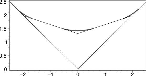
Figure 10: An $N=3$ example of the limit shape

5.2.3 The Seiberg-Witten family of curves

The conformal map $\Phi$ can be written down explicitly, namely it is a linear function of $\log w$, where $w=w(z)$ solves the equation

$$w+\frac{1}{w}=z^{N}+0\cdot z^{N-1}+\dots\,.$$ (5.9)

Here dots stand for a certain polynomial of degree $N-2$ in $z$ which is to be found from the slit-lengths and, ultimately, from the $u_{i}$’s. The equation (5.9) defines an $(N-1)$-dimensional family of hyperelliptic curves of genus $N-1$. These curves are known as the Seiberg-Witten curves. They also arise as spectral curves in the periodic Toda chain (there is, in fact, a natural connection between periodically weighted Plancherel measure and periodic Toda chain).

The $N-1$ gap-periods of the differential (5.7) can be taken as local coordinates on the family (5.9). The main feature of the Seiberg-Witten geometry is that the dual band-periods of (5.7) turn out to be the dual variables for the Legendre transform of the prepotential $S(f^{\star})$. This follows from Theorem 4 by a direct simple computation, see [67], and completes the derivation of the Seiberg-Witten geometry.

Princeton University
Department of Mathematics
Fine Hall, Washington Road,
Princeton, New Jersey 08544, U.S.A.
okounkov@math.princeton.edu

References

- [1] M. Adler and P. van Moerbeke, Integrals over classical groups, random permutations, Toda and Toeplitz lattices, Comm. Pure Appl. Math. 54 (2001), no. 2, 153–205.
- [2] M. Atiyah and R. Bott, The moment map and equivariant cohomology, Topology 23 (1984), 1-28.
- [3] J. Baik, P. Deift, K. Johansson, On the distribution of the length of the longest increasing subsequence of random permutations, Journal of AMS, 12 (1999), 1119–1178.
- [4] J. Baik, P. Deift, E. Rains, A Fredholm determinant identity and the convergence of moments for random Young tableaux, Comm. Math. Phys. 223 (2001), no. 3, 627–672.
- [5] J. Baik, E. Rains, The asymptotics of monotone subsequences of involutions, Duke Math. J. 109 (2001), no. 2, 205–281.
- [6] P. Biane, Representations of symmetric groups and free probability, Adv. Math., 138, 1998, no. 1, 126–181.
- [7] S. Bloch and A. Okounkov, The Character of the Infinite Wedge Representation, Adv. Math. 149 (2000), no. 1, 1–60.
- [8] A. Borodin, A. Okounkov, and G. Olshanski, Asymptotics of the Plancherel measures for symmetric groups, J. Amer. Math. Soc. 13 (2000), no. 3, 481–515.
- [9] A. Borodin and G. Olshanski, Point processes and the infinite symmetric group, Math. Res. Lett. 5 (1998), no. 6, 799–816.
- [10] A. Borodin and G. Olshanski, Distribution on partitions, point processes, and the hypergeometric kernel, Comm. Math. Phys. 211 (2000), no. 2, 335–358.
- [11] E. Brézin and V. Kazakov, Exactly solvable field theories of closed strings, Phys. Let. B236 (1990), 144-150.
- [12] T. Britz and S. Fomin, Finite posets and Ferrers shapes, Adv. Math. 158 (2001), no. 1, 86–127.
- [13] W. Burnside, Theory of groups of finite order, 2nd edition, Cambridge University Press, 1911.
- [14] P. Deift, Orthogonal Polynomials and Random Matrices: A Riemann-Hilbert Approach, AMS 2000.
- [15] P. Di Franceso, 2-d quantum gravities and topological gravities, matrix models, and integrable differential systems, in The Painlevé property: one century later, (R. Conte, ed.), 229-286, Springer: New York, 1999.
- [16] P. Di Franceso, P. Ginzparg, and J. Zinn-Justin, 2D Quantum gravity and random matrix models, Phys. Rep. 254 (1995). 1–131.
- [17] P. Di Franceso, C. Itzykson, and J. B. Zuber, Polynomial averages in the Kontsevich model, Comm. Math. Phys., 151 (1993), 193–219.
- [18] R. Dijkgraaf, Mirror symmetry and elliptic curves, The Moduli Space of Curves, R. Dijkgraaf, C. Faber, G. van der Geer (editors), Progress in Mathematics, 129, Birkhäuser, 1995.
- [19] R. Donagi, Seiberg-Witten integrable systems, Algebraic geometry—Santa Cruz 1995, 3–43, Proc. Sympos. Pure Math., 62, Part 2, Amer. Math. Soc., Providence, RI, 1997.
- [20] M. Douglas, Strings in less than one dimension and generalized KP hierarchies, Phys. Let. B238 (1990)
- [21] M. Douglas and S. Schenker, Strings in less than one dimension, Nucl. Phys. B335 (1990).
- [22] T. Eguchi, K. Hori, and S.-K. Yang, Topological models and large- matrix integral, Internat. J. Modern Phys. A 10 (1995), no. 29, 4203–4224.
- [23] T. Eguchi and S.-K. Yang, The topological model and the large-N matrix integral, Mod. Phys. Lett. A 9 (1994), 2893–2902.
- [24] T. Ekedahl, S. Lando, M. Shapiro, and A. Vainshtein, Hurwitz numbers and intersections on moduli spaces of curves, Invent. Math. 146 (2001), no. 2, 297–327.
- [25] A. Eskin, H. Masur, A. Zorich, Moduli Spaces of Abelian Differentials: The Principal Boundary, Counting Problems and the Siegel–Veech Constants, math.DS/0202134.
- [26] A. Eskin, A. Okounkov, Asymptotics of numbers of branched coverings of a torus and volumes of moduli spaces of holomorphic differentials, Invent. Math. 145 (2001), no. 1, 59–103.
- [27] C. Faber and R. Pandharipande, Hodge integrals and Gromov-Witten theory, Invent. Math. 139 (2000), 173-199.
- [28] W. Fulton and R. Pandharipande, Notes on stable maps and quantum cohomology, in Proceedings of symposia in pure mathematics: Algebraic Geometry Santa Cruz 1995 Volume 62, Part 2 (J. Kollár, R. Lazarsfeld, and D. Morrison, eds.), 45-96, AMS: Rhode Island, 1997.
- [29] E. Getzler, The Toda conjecture, Symplectic geometry and mirror symmetry (Seoul, 2000), 51–79, World Sci. Publishing, River Edge, NJ (2001), math.AG/0108108.
- [30] E. Getzler, The equivariant Toda conjecture, math.AG/0207025.
- [31] D. Gross and A. Migdal, Nonperturbative two-dimensional quantum gravity, Phys. Rev. Lett. 64 (1990)
- [32] D. Gross and A. Migdal, A nonperturbative treatment of two-dimensional quantum gravity, Nucl. Phys. B340 (1990), 333–365.
- [33] M. Haiman, Notes on Macdonald polynomials and the geometry of Hilbert schemes, Proceedings of the NATO Advanced Study Institute held in Cambridge, June 25–July 6, 2001, Sergey Fomin, ed. Kluwer, Dordrecht (2002) 1–64.
- [34] J. Harer and D. Zagier, The Euler characteristic of the moduli space of curves, Invent. Math., 85, 1986, 457–485.
- [35] J. Haris, I. Morrison, Moduli of curves, Springer-Verlag, 1998.
- [36] A. Hurwitz, Über die Anzahl der Riemann’schen Flächen mit gegebenen Verzweigungspunkten, Math. Ann. 55 (1902), 53-66.
- [37] C. Itzykson, and J. B. Zuber, Combinatorics of the modular group. 2. The Kontsevich integral, Int. J. Mod. Phys. A7 (1992), 1–23.
- [38] K. Johansson, The longest increasing subsequnce in a random permutation and a unitary random matrix model, Math. Res. Lett., 5 (1998), no. 1-2, 63–82.
- [39] K. Johansson, Discrete orthogonal polynomial ensembles and the Plancherel measure, Ann. of Math. (2) 153 (2001), no. 1, 259–296.
- [40] K. Johansson, Non-intersecting paths, random tilings and random matrices, Probab. Theory Related Fields 123 (2002), no. 2, 225–280.
- [41] G. Jones, Characters and surfaces: a survey The atlas of finite groups: ten years on (Birmingham, 1995), 90–118, London Math. Soc. Lecture Note Ser., 249, Cambridge Univ. Press, Cambridge, 1998.
- [42] V. Kac, Infinite dimensional Lie algebras, Cambridge University Press.
- [43] V. Kac and A. Schwarz, Geometric interpretation of the partition function of 2D gravity, Physics Letters B 257 (1991), 329–334.
- [44] R. Kenyon, A. Okounkov, S. Sheffield, in preparation.
- [45] S. Kerov, Gaussian limit for the Plancherel measure of the symmetric group, C. R. Acad. Sci. Paris, 316, Série I, 1993, 303–308.
- [46] S. Kerov, Transition probabilities of continual Young diagrams and the Markov moment problem, Func. Anal. Appl., 27, 1993, 104–117.
- [47] S. Kerov, The asymptotics of interlacing roots of orthogonal polynomials, St. Petersburg Math. J., 5, 1994, 925–941.
- [48] S. Kerov, A differential model of growth of Young diagrams, Proceedings of the St. Petersburg Math. Soc., 4, 1996, 167–194.
- [49] S. Kerov, Interlacing measures, Amer. Math. Soc. Transl., 181, Series 2, 1998, 35–83.
- [50] S. Kerov, Asymptotic Representation Theory of the Symmetric Group and its Applications in Analysis, AMS, 2003.
- [51] S. Kerov and G. Olshanski, Polynomial functions on the set of Young diagrams, C. R. Acad. Sci. Paris Sér. I Math., 319, no. 2, 1994, 121–126.
- [52] M. Kontsevich, Intersection theory on the moduli space of curves and the matrix Airy function, Comm. Math. Phys. 147 (1992), 1-23.
- [53] A. Lascoux and J.-Y. Thibon, Vertex operators and the class algebras of symmetric groups, Zap. Nauchn. Sem. S.-Peterburg. Otdel. Mat. Inst. Steklov. (POMI) 283 (2001), Teor. Predst. Din. Sist. Komb. i Algoritm. Metody 6, 156–177.
- [54] B. F. Logan and L. A. Shepp, A variational problem for random Young tableaux, Adv. Math., 26, 1977, 206–222.
- [55] E. Looijenga, Intersection theory on Deligne-Mumford compactifications (after Witten and Kontsevich), Séminaire Bourbaki, Vol. 1992/93. Ast risque No. 216, (1993), Exp. No. 768, 4, 187-212.
- [56] A. Losev, N. Nekrasov, S. Shatashvili, Issues in Topological Gauge Theory, Nucl. Phys. B534 (1998) 549–611.
- [57] A. Losev, N. Nekrasov, S. Shatashvili, Testing Seiberg-Witten Solution, hep-th/9801061.
- [58] I. G. Macdonald, Symmetric functions and Hall polynomials, Clarendon Press, 1995.
- [59] M. Mehta, Random matrices, Academic Press, 1991.
- [60] T. Miwa, M. Jimbo, E. Date, Solitons. Differential equations, symmetries and infinite-dimensional algebras, Cambridge Tracts in Mathematics, 135. Cambridge University Press, Cambridge, 2000.
- [61] P. van Moerbeke, Random matrices and permutations, matrix integrals and integrable systems, Séminaire Bourbaki, Vol. 1999/2000, Astérisque 276 (2002), 411–433.
- [62] P. van Moerbeke, Integrable lattices: random matrices and random permutations. Random matrix models and their applications, 321–406, Math. Sci. Res. Inst. Publ., 40, Cambridge Univ. Press, Cambridge, 2001.
- [63] H. Nakajima, Lectures on Hilbert schemes of points on surfaces, AMS 1999
- [64] H. Nakajima, K. Yoshioka, Instanton counting on blowup, I, math.AG/0306198.
- [65] N. Nekrasov, Seiberg-Witten Prepotential From Instanton Counting, hep-th/0206161.
- [66] N. Nekrasov, ICMP 2003 contribution, this volume.
- [67] N. Nekrasov, A. Okounkov, Seiberg-Witten Theory and Random Partitions, hep-th/0306238.
- [68] A. Okounkov, Random matrices and random permutations Internat. Math. Res. Notices 2000, no. 20, 1043–1095.
- [69] A. Okounkov, Infinite wedge and random partitions, Selecta Math., New Ser., 7 (2001), 1–25.
- [70] A. Okounkov, Generating functions for intersection numbers on moduli spaces of curves, Internat. Math. Res. Notices, no. 18 (2002) 933–957.
- [71] A. Okounkov, Symmetric function and random partitions, Proceedings of the NATO Advanced Study Institute held in Cambridge, June 25–July 6, 2001, Sergey Fomin, ed. Kluwer, Dordrecht (2002) 1–64.
- [72] A. Okounkov and R. Pandharipande, Gromov-Witten theory, Hurwitz numbers, and matrix models, I, math.AG/0101147.
- [73] A. Okounkov and R. Pandharipande, Gromov-Witten theory, Hurwitz theory, and completed cycles, math.AG/0204305.
- [74] A. Okounkov and R. Pandharipande, The equivariant Gromov-Witten theory of , math.AG/0207233.
- [75] A. Okounkov and R. Pandharipande, Virasoro constraints for target curves, math.AG/0308097.
- [76] R. Pandharipande, The Toda equations and the Gromov-Witten theory of the Riemann sphere, Lett. Math. Phys. 53 (2000), no. 1, 59–74.
- [77] M. Prähofer and H. Spohn, Universal Distributions for Growth Processes in 1+1 Dimensions and Random Matrices, Phys. Rev. Lett. 84, 4882 (2000).
- [78] M. Prähofer and H. Spohn, Scale invariance of the PNG droplet and the Airy process, J. Statist. Phys. 108 (2002), no. 5-6, 1071–1106.
- [79] E. M. Rains, Increasing subsequences and the classical groups, Electr. J. of Combinatorics, 5(1), 1998.
- [80] B. Sagan, The symmetric group. Representations, combinatorial algorithms, and symmetric functions, Springer-Verlag, 2001.
- [81] G. Segal and G. Wilson, Loop groups and equations of KdV type, Inst. Hautes Études Sci. Publ. Math. No. 61, (1985), 5–65.
- [82] N. Seiberg, E. Witten, Monopole Condensation, And Confinement In Supersymmetric Yang-Mills Theory, Nucl.Phys. B426 (1994) 19–52; Erratum-ibid. B430 (1994) 485–486.
- [83] N. Seiberg, E. Witten, Monopoles, Duality and Chiral Symmetry Breaking in Supersymmetric QCD, Nucl.Phys. B431 (1994) 484–550.
- [84] T. Seppäläinen, A microscopic model for Burgers equation and longest increasing subsequences, Electron. J. Prob., 1, no. 5, 1996.
- [85] C. A. Tracy and H. Widom, Level-spacing distributions and the Airy kernel, Commun. Math. Phys., 159, 1994, 151–174.
- [86] C. Tracy and H. Widom Random Unitary Matrices, Permutations and Painleve, Comm. Math. Phys. 207 (1999), no. 3, 665–685.
- [87] C. Tracy and H. Widom, On the Distributions of the Lengths of the Longest Monotone Subsequences in Random Words, Probab. Theory Related Fields 119 (2001), no. 3, 350–380.
- [88] K. Ueno and K. Takasaki, Toda lattice hierarchy, Adv. Studies in Pure Math. 4, Group Representations and Systems of Differential Equations, 1–95, 1984.
- [89] A. Vershik, Statistical mechanics of combinatorial partitions and their limit configurations, Func. Anal. Appl., 30, no. 2, 1996, 90–105.
- [90] A. Vershik and S. Kerov, Asymptotics of the Plancherel measure of the symmetric group and the limit form of Young tableaux, Soviet Math. Dokl., 18, 1977, 527–531.
- [91] A. Vershik and S. Kerov, Asymptotic theory of the characters of a symmetric group, Functional Anal. Appl. 15 (1981), no. 4, 246–255.
- [92] A. Vershik and S. Kerov, Asymptotics of the maximal and typical dimension of irreducible representations of symmetric group, Func. Anal. Appl., 19, 1985, no.1.
- [93] E. Witten, Two dimensional gravity and intersection theory on moduli space, Surveys in Diff. Geom. 1 (1991), 243-310.
- [94] A. Zvonkin, Matrix integrals and map enumeration: an accessible introduction, Math. Comput. Modelling, 26, 1997, no. 8–10, 281–304.