Abstract

We identify the scaling region of a width $O(n^{-1})$ in the vicinity of the accumulation points $t=\pm 1$ of the real roots of a random Kac-like polynomial of large degree $n$. We argue that the density of the real roots in this region tends to a universal form shared by all polynomials with independent, identically distributed coefficients $c_{i}$, as long as the second moment $\sigma=\mbox{\bf E}(c_{i}^{2})$ is finite. In particular, we reveal a gradual (in contrast to the previously reported abrupt) and quite nontrivial suppression of the number of real roots for coefficients with a nonzero mean value $\mu_{n}=\mbox{\bf E}(c_{i})$ scaled as $\mu_{n}\sim n^{-1/2}$.

1 Introduction

Recently, there was an essential resurrection of interest in statistical properties of zeros of random polynomials and random analytic functions [1]–[15].

The distribution of real roots for random polynomials was studied in classical papers by Bloch and Polya [16], Littlewood and Offord [17], Kac [18] and many others. Many results and an overview of the field is given in the recent monograph by Farahmand [22].

As is well-known, for the case of algebraic polynomials

$$f_{n}(t)=c_{0}+c_{1}t+...+c_{n-1}t^{n-1}$$ (1.1)

where the real coefficients $c_{i}$ are independently and identically distributed around mean zero, the roots are mostly located near $\pm 1$. A natural intuitive picture for such an accumulation was proposed by Kac. Indeed, if all coefficients $c_{i}$ are of the same order then only for $|t|=1$ will the terms have a good chance to interact and cancel each other producing zero.

In particular, for Gaussian-distributed coefficients with mean $E[c_{j}]=0$ and variance $E[c_{j}^{2}]=\sigma$, the mean density of real zeros of an algebraic polynomial $p_{n}(t)$ is given by the Kac formula

$$p_{n}(t)=\frac{\sqrt{A_{n}(t)C_{n}(t)-B_{n}^{2}(t)}}{\pi A_{n}(t)}$$ (1.2)

where

$$A_{n}(t)=\sigma\sum_{j=0}^{n-1}t^{2j}=\sigma\frac{t^{2n}-1}{t-1}\,,\quad B_{n}(t)=\frac{1}{2}\frac{d}{dt}A_{n}(t)\,,\quad C_{n}(t)=\frac{1}{4}\frac{d^{2}}{dt^{2}}A_{n}(t)+\frac{1}{4t}\frac{d}{dt}A_{n}(t)\,.$$

Usually, one is interested in the limit of polynomials of high degree $n$. For a fixed $t$ the density is given by:

$$\lim_{n\to\infty}p^{(f)}_{n}(t\neq\pm 1)=p^{(f)}(t)=\frac{1}{\pi|1-t^{2}|}$$ (1.3)

and

$$p_{n}(\pm 1)=\frac{1}{\pi}\left[\frac{n^{2}-1}{12}\right]^{1/2}$$

The expected number of real zeros is known to have the following asymptotics:

$$N_{n}(-\infty,\infty)=\int_{-\infty}^{\infty}p_{n}(t)dt=\frac{2}{\pi}\log{n}+C+O(n^{-2})$$ (1.4)

where the leading logarithmic term was found by Kac himself, and the corrections, in particular, the constant

$$C=\frac{2}{\pi}\left\{\int_{0}^{1}\sqrt{\frac{1}{v^{2}}-\frac{1}{\sinh^{2}{v}}}\,dv-\int_{1}^{\infty}\left[\frac{1}{t}-\sqrt{\frac{1}{v^{2}}-\frac{1}{\sinh^{2}{v}}}\;\right]\,dv\right\}$$ (1.5)

was found by Wilkins [20]. In fact, the asymptotic result $N_{n}(-\infty,\infty)=\frac{2}{\pi}\log{n}$ was proven to be very universal, i.e. insensitive to the details of the distribution of coefficients $c_{i}$, see discussion and further references in [22]. A similar universality result is also available for the variance of the total number of real zeros [21].

The nature of the informal arguments by Kac suggests that close to the values $t=\pm 1$ many random terms of comparable magnitude add up to form the polynomial, and the emerging object should be universal in the spirit of the central limit theorem.

Another natural question arises about the expected number of real zeros for coefficients with a nonvanishing mean value E$[c_{i}]=\mu$. It is straightforward to include the mean value to the standard derivation of the Kac formula for gaussian-distributed coefficients and arrive at the following expression:

$$p_{n}^{\mu}(t)=p_{n}(t)e^{-\frac{1}{2}\left[\Sigma_{1}(t)+\Sigma_{2}(t)\right]}\int_{0}^{\infty}dq\;q\cosh{\left(q\sqrt{\Sigma_{1}(t)}\right)}e^{-\frac{q^{2}}{2}}$$ (1.6)

$$\Sigma_{1}(t)=\frac{A_{n}(t)D^{2}_{n}(t)}{A_{n}(t)C_{n}(t)-B_{n}^{2}(t)}\quad,\quad\Sigma_{2}(t)=\frac{G^{2}_{n}(t)}{A_{n}(t)}$$ (1.7)

where

$$D_{n}(t)=-G_{n}(t)\frac{B_{n}(t)}{A_{n}(t)}+\frac{d}{dt}G_{n}(t)\quad,\quad G_{n}(t)=\mu\sum_{j=0}^{n-1}t^{j}=\mu\frac{t^{n}-1}{t-1}$$ (1.8)

and $P_{n}(t),A_{n}(t),B_{n}(t)$ and $C_{n}(t)$ are defined in (1.2).

Earlier investigation [22] has revealed that any, whatever small, mean value $\mu>0$ asymptotically, for large $n$, kills exactly half of real zeros and converts the above quoted result 1.4 for their number into $N_{n}(-\infty,\infty)=\frac{1}{\pi}\log{n}$. It is this surprising abruptness that motivated us to have a closer look at the origin of such a behavior. This question turned out to be also related to exploring the appropriately scaled vicinity of the accumulation points.

2 Scaling and Universality

It is quite clear (and can be verified numerically) that the root density function $p_{n}(t)$ as well as its limiting form (1.3) are both not universal. On other hand, the essence of the Kac argument discussed above and the mentioned universality of $N_{n}(-\infty,\infty)$ suggests that universal features have to emerge in close vicinity of the accumulation points $t=\pm 1$. In fact, it is easy to understand that the relevant vicinity of $|t|=1$ is of the order of $n^{-1}$ for large degree $n$. We will refer to such domain as the ’local scaling regime’, as opposed to keeping the distance $|1\pm t|$ from the accumulation points $t=\pm 1$ fixed in the limit $n\to\infty$, the latter regime being referred to as the ’global’ one. In particular, our main goal is to verify Proposition 2.1.

Proposition 2.1.

Let coefficients $\{c_{j}\}^{n-1}_{j=0}$ of a random polynomial $f_{n}(t)$ be i.i.d real random variables with ${\bf E}[c_{j}]=\mu_{n}>0$ and finite variance chosen to be unity: ${\bf E}[c_{j}^{2}]=1$. Let $N_{n}(x_{1},x_{2})$ be the number of real zeros of $f_{n}(t)$ in the interval $\left[1-\frac{x_{2}}{n}\,,\,1-\frac{x_{1}}{n}\right]$, with $0\leq x_{1}<x_{2}<n$. Then

$$\lim_{n\to\infty}{\bf E}\left[N_{n}(x_{1},x_{2})\right]=\int_{x_{1}}^{x_{2}}p_{\alpha}(v)\,dv$$ (2.9)

where $\alpha=\lim_{n\to\infty}(n\mu_{n}^{2})$ and the density function $p_{\alpha}(v)$ is given by

$$p_{\alpha}(v)=\frac{1}{\pi}\sqrt{\frac{1}{v^{2}}-\frac{1}{\sinh^{2}{v}}}e^{-\alpha J(v)}\int_{0}^{\infty}dq\;q\cosh{\left(q\sqrt{\alpha M(v)}\right)}e^{-\frac{q^{2}}{2}}$$ (2.10)

$$J(v)=\frac{\sinh^{2}{(v/2)}}{(v/2)^{2}}\frac{1}{1+\sinh{v}/{v}}\quad\quad M(v)=\frac{\sinh{v}/{v}}{\cosh^{2}{(v/2)}}\frac{1-\sinh{v}/{v}}{1+\sinh{v}/{v}}$$ (2.11)

A similar statement is valid for the vicinity of second accumulation point $t=-1$ for $\mu_{n}<0$.

Here we present explicit arguments in favour of the validity of such a proposition for the simplest case $\mu_{n}=0$. The ’local regime’ formula (2.10) reduces in that case to the following simple expression:

$$p_{0}(v)=\frac{1}{2\pi}\sqrt{\frac{1}{v^{2}}-\frac{1}{\sinh^{2}{v}}}$$ (2.12)

The modifications required to include nonzero mean $\mu_{n}$ are self-evident and left to the reader.

Our starting formula is the following representation for the number of real roots $N_{n}(x_{1},x_{2})$ of $f_{n}(t)$ in the interval $\left[1-\frac{x_{2}}{n}\,,\,1-\frac{x_{1}}{n}\right]$, see e.g. [6, 22]:

$$N_{n}(x_{1},x_{2})=\int_{1-\frac{x_{2}}{n}}^{1-\frac{x_{1}}{n}}\,dt\int_{-\infty}^{\infty}dy\,|y|\,{\cal D}_{n}(0,y;t)$$ (2.13)

where

$${\cal D}_{n}(x,y;t)=\mbox{\bf E}\left[\delta\left(x-\sum_{j=0}^{n-1}c_{j}t^{j}\right)\delta\left(y-\sum_{j=0}^{n-1}jc_{j}t^{j-1}\right)\right]$$ (2.14)

stands for the joint probability density of the random polynomial $f_{n}(t)$ and its derivative over $t$. Let us introduce in the above representation the scaling variables $v$, $\tilde{x}$ and $\tilde{y}$ by relations:

$$t=1-v/n\qquad x=n^{1/2}\tilde{x}\qquad y=n^{3/2}\tilde{y}.$$

Changing the variables of integration one finds:

$$N_{n}(x_{1},x_{2})=\int_{x_{1}}^{x_{2}}\,dv\int_{-\infty}^{\infty}d\tilde{y}\,|\tilde{y}|\,\tilde{{\cal D}}_{n}(0,\tilde{y};v)$$ (2.15)

where

$$\tilde{{\cal D}}_{n}(\tilde{x},\tilde{y};v)=\mbox{\bf E}\left[\delta\left(\tilde{x}-\frac{1}{n^{1/2}}\sum_{j=0}^{n-1}c_{j}(1-v/n)^{j}\right)\delta\left(\tilde{y}-\frac{1}{n^{3/2}}\sum_{j=0}^{n-1}jc_{j}(1-v/n)^{j-1}\right)\right]\,.$$ (2.16)

Evidently each of the scaled random variables $\tilde{x}$ and $\tilde{y}$ is a sum of $n$ independent, although not identically distributed terms, with the magnitude of fluctuations of each term depending on the summation index $j$. Calculating the variances of the scaled variables we find that they are given by

$$A_{n}(v)=\mbox{\bf E}\left[\tilde{x}^{2}\right]=\frac{1}{n}\sum_{j=0}^{n-1}(1-v/n)^{2j}=\frac{1-(1-v/n)^{2n}}{v(2-v/n)}$$ (2.17)

and

$$B_{n}(v)=\mbox{\bf E}\left[\tilde{y}^{2}\right]=\frac{1}{n^{2}}\sum_{j=0}^{n-1}j(1-v/n)^{2j-1}=\frac{1}{2n^{2}}\frac{d}{da}\left(\frac{a^{n}-1}{a-1}\right)_{a=(1-v/n)^{2}}$$ (2.18)

and their covariance is just

$$C_{n}(v)=\mbox{\bf E}\left[\tilde{x}\tilde{y}\right]=\frac{1}{n^{3}}\sum_{j=0}^{n-1}j^{2}(1-v/n)^{2j-2}=\frac{1}{n^{3}}\frac{d}{da}\left[a\frac{d}{da}\left(\frac{a^{n}-1}{a-1}\right)\right]_{a=(1-v/n)^{2}}\,.$$ (2.19)

We further notice that all three quantities $A_{n}(v)$, $B_{n}(v)$ and $C_{n}(v)$ have a well-defined finite large $n$ limit:

$$A_{n}(v)\to A_{\infty}=\frac{1-e^{-2v}}{2v}\;\quad\qquad B_{n}(v)\to B_{\infty}=-\frac{1}{2}\frac{dA_{\infty}}{dv}\;\quad\qquad C_{n}(v)\to C_{\infty}=\frac{1}{4}\frac{d^{2}A_{\infty}}{dv^{2}}$$ (2.20)

coinciding with the limiting values of $A,B,C$ in Eq.(1.2) after rescaling $t=1-v/n$ and the limit $n\to\infty$ for a fixed $v$. Now invoking the local central limit theorem [26] we infer that the limiting joint probability density $\tilde{D}_{\infty}$ of the scaled variables $\tilde{x}$ & $\tilde{y}$ tends when $n\to\infty$ to the normal law with variances $A_{\infty},B_{\infty}$ and covariance $C_{\infty}$, as if the polynomial coefficients were normal with unit variance. Therefore, the Kac formula for the density of real roots should be asymptotically valid in this case, and the formula Eq.(2.12) immediately follows after substituting those limiting values into the Kac expression Eq.(1.2). Separation of the two regimes and identification of the scaling is in some sense similar to ’local’ versus ’global’ scaling regimes in spectra of random matrices. Only when the spectral parameters are scaled appropriately will the various correlation functions characterising the eigenvalues of large random matrices show a surprisingly robust universality [24, 25].

Although the expressions Eq.(2.10), and especially Eq.(2.12) look very natural (cf. the structure of the asymptotic result Eq.(1.4)) and their universality stems from such basic fact as the central limit theorem, we failed to trace a similar statement in the available literature on random polynomials with real coefficients. For complex zeros a kind of ’local’ regime was studied in much detail by Shepp & Vanderbei [3] and Ibragimov & Zeitouni [8] who showed that those zeros tend to concentrate asymptotically on the unit circle. Only very recently (squared) expression of the type (2.12) independently emerged in studies of complex zeros of polynomials with complex i.i.d. coefficients, see Shiffman and Zelditch, [15]. A different kind of universality results was addressed in a very recent paper [7] which appeared when the present paper was under completion.

3 Numerical Examples, Discussion and Perspectives

It is interesting and informative to have a look at the profiles of the real root density in the ’local scaling regime’ around the point $t=1$ (i.e $v=0$) for some typical values of the parameters, and compare them with the results of numerical simulations. In fig. (1) we plotted the density profiles obtained by a direct numerical search for real roots of polynomials with gaussian-distributed coefficients for degrees $n=100$, $300$ & $1000$. The (scaled) mean value $\alpha_{n}=\mu_{n}^{2}n$ of the coefficients was chosen to be $\alpha=10$ and the variance was always kept unity. The results can be compared with both the exact predictions of the Kac-type formula (1.6) for the same values of $n,\sigma$ and $\mu_{n}=\sqrt{\alpha/n}$, and with the asymptotic universal profile of (2.10).

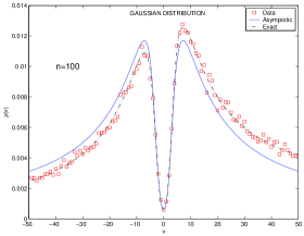
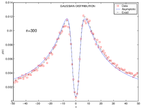
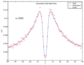
Figure 1: Numerical vs. analytical density profiles for real roots of polynomials with gaussian-distributed coefficients. Each data set corresponds to $100,000$ realisations of random polynomials.

It is trivial to see that as $n$ increases the exact Kac-like expression begins to coincide with the asymptotic profile, and the analytical curve agrees well with the numerical data. To verify universality we also performed numerical simulations for the case of coefficients uniformly distributed in the interval of the widths $1/\sqrt{3}$ around the same mean values $\mu_{n}$. The picture looks very similar, see fig. (2), and again agreement with the asymptotic formula for large values of $n$ is very good.

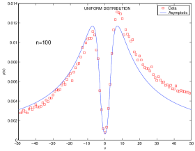
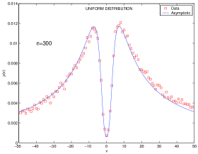
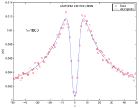
Figure 2: Numerical data versus asymptotic density profile (2.10) for the uniformly distributed coefficients. Each data set corresponds to $100,000$ realisations of random polynomials.

One can notice a couple of interesting features. First simple observation is that the exact Kac formulae are asymmetric about $v=0$ for ’small’ $n$ (in the ’local regime’) but it becomes ”asymptotically symmetric” with increasing $n$, as predicted by (2.10). This feature is easy to understand in view of the global inversion symmetry $t\to t^{-1}$ which holds exactly for all polynomials with i.i.d. coefficients. In the local regime close to accumulation points this symmetry implies the asymptotic reflection symmetry $v\to-v$.

The most surprising feature is a non-trivial double-peak structure of the density profile, and it deserves to be discussed in more detail.

In fact, it turns out that as $\alpha$ increases the shape of the density profile described by formula (2.10) changes from that with one maximum to that with two symmetric maxima as illustrated in the fig. (3).

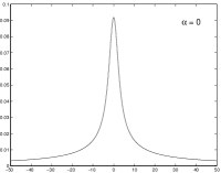
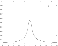
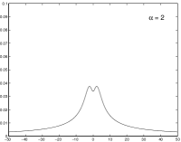
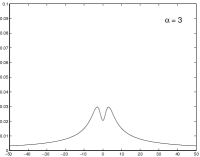
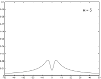
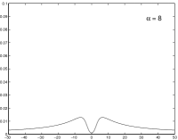
Figure 3: Suppression of the density profile by increasing scaled mean value $\alpha$ from $0$ to $8$ for a degree 100 polynomial.

This fact can be verified analytically by considering the small-$v$ expansion:

$$p_{\alpha}(v)=\frac{1}{\pi\sqrt{3}}\;e^{-\alpha/2}\left[1-\frac{v^{2}}{2}\left(\frac{1}{5}-\frac{1}{6}\;\alpha\right)+\frac{v^{4}}{36}\left(\frac{137}{350}-\frac{5}{8}\;\alpha+\frac{1}{12}\;\alpha^{2}\right)+O(v^{5})\right]$$ (3.21)

valid for $\alpha v^{2}\ll 1$. We see that for $\alpha>\alpha_{c}=6/5$ the local maximum at $v=0$ is converted to a minimum. On the other hand, for $|v|\gg\alpha$ we easily find from Eq.(2.10) the $\alpha-$independent far tail decay law $p_{\alpha}(v)\approx 1/{\pi|v|}$ which ensures that at least two symmetric maxima have to appear at $v\neq 0$. Notice that the far tail values are much larger for $\alpha\gg 1$ than the exponentially small density $p_{\alpha}(0)=\frac{1}{\pi\sqrt{3}}\;e^{-\alpha/2}$ at the origin, and thus the maxima have to be quite pronounced.

The precise reason for such a nonmonotonous behavior is not clear to us at the moment, and deserve further investigations. We consider that feature as an indication of a rather nontrivial statistics of zeros accumulating in the scaling region around the points $\pm 1$.

Fixing the value of $\mu$ and performing the limit $n\to\infty$ amounts to letting $\alpha\to\infty$. This results in vanishing density of the real roots $p_{\alpha}(v)\to 0$ for any fixed $v$. This fact corresponds to observed suppression of exactly half of the real zeros (the vicinity of the second accumulation point is not at all affected by the nonvanishing mean $\mu_{n}$). In contrast, correctly tuning the mean value with the parameter $n$ by letting $\mu_{n}\sim n^{-1/2}$ and magnifying the vicinity of the accumulation point via the correct scaling $1-t\sim n^{-1}$ results in a density function (2.10) and thus describes a gradual (as opposed to abrupt) suppression of real zeros in the scaling regime, see fig. (3).

Let us now briefly discuss open questions and perspectives for further research.

A very interesting development of the theory of random polynomials comes from the paper by Bleher and Di [6]. The authors discovered nontrivial correlations between positions of real zeros of algebraic polynomials. The correlations can be conveniently characterised by correlation functions of the polynomial zeros:

$$K(t_{1},...,t_{l})=\lim_{n\to\infty}{\bf E}\left[\lim_{\Delta_{1},...,\Delta_{l}\to 0}\frac{N^{(f)}(t_{1},t+\Delta_{1})...N^{(f)}(t_{l},t_{l}+\Delta_{l})}{|\Delta_{1}|...|\Delta_{l}|}\right]$$ (3.22)

where $N^{(f)}(a,b)$ is the number of real zeros of the polynomial $f(t)$ in the interval $[a,b]$.

The consideration of correlation functions studied by Bleher and Di was restricted, in our terminology, to the ’global regime’. It should be possible to derive ’local regime’ formulae for those quantities. The expressions are expected to be universal in the same sense as the ’local regime’ formula for expected number of roots, Eqs. (2.9, 2.10). The simplest nontrivial quantity of that type should be the variance $var{\left[N_{n}(x_{1},x_{2})\right]}$ of the number of real roots in the vicinity of $t=1$.

Another natural object to study is the variation of the number of real polynomial roots against a small change of the vector of real coefficients ${\bf c}=c_{0},...,c_{n-1}$. More specifically, change ${\bf c}\to{\bf c}_{v}={\bf c}+v{\bf b}$ assuming the components of the vector ${\bf b}$ to be i.i.d. standard Gaussian. The parameter $v\geq 0$ is used here to control the magnitude of the perturbation. By using $f_{v}(t)$ to denote the perturbed polynomial an interesting question arises, that is can we generalize the correlation functions Eq.(3.22) to the following parametric correlation functions:

$$K_{v_{1},...,v_{l}}(t_{1},...,t_{l})=\lim_{n\to\infty}{\bf E}\left[\lim_{\Delta_{1},...,\Delta_{l}\to 0}\frac{N^{(f_{v_{1}})}(t_{1},t+\Delta_{1})...N^{(f_{v_{l}})}(t_{l},t_{l}+\Delta_{l})}{|\Delta_{1}|...|\Delta_{l}|}\right]$$ (3.23)

which reflects the change in the positions of the real roots. Similar objects are of interest in the theory of random matrices and disordered systems (see [27] and references therein).

As a preliminary step of our research we evaluated the simplest nontrivial parametric correlation function, following the paper [6] and found in the ’local regime’:

$$\frac{K_{0,v}(t,t)}{[p(t)]^{2}}=1+\frac{1}{v}\arcsin{\frac{1}{\sqrt{1+v^{2}}}}$$

It will be interesting to attack the problem in full generality, both for ’global’ and especially for ’local’ regime, where the results are expected to be universal.

In fact, our initial interest in the properties of random polynomials was stimulated by the fact that closely related methods can be applied to study the properties of irregular eigenfunctions in ’quantum billiards.’ The eigenfunctions $\Psi(x,y)$ at the point with the coordinate vector $\vec{r}=(x,y)$ are solutions of the Helmholtz equation: $-\Delta\Psi(\vec{r})=E\Psi(\vec{r})\quad;\quad\vec{r}\in\Omega$ where $\Omega$ is a connected compact domain with the boundary $\partial\Omega$, and $\Delta$ is the Laplacian.

Recently Smilansky and collaborators [23] suggested looking for the eigenfunctions at the point $\vec{r}$ in the following representation:

$$\Psi(r,\theta)=\sum_{l=-L}^{L}a_{l}J_{l}(k|r|)e^{il\theta}\;$$ (3.24)

where $J_{l}(x)$ stands for the Bessel functions, $r,\theta$ are polar coordinates of the observation point, and the integer $L$ is given in terms of the wavenumber $k$ and the perimeter $D$ of the billiard boundary $\partial\Omega$ as $L=\frac{1}{2}\left[\frac{kD}{\pi}\right]$. The complex coefficients $a_{l}$ satisfying $\overline{a_{l}}=(-1)^{l}a_{-l}$ are taken to be i.i.d. complex Gaussian variables with unit variance, in accordance to The Berry’s conjecture. Based on such a formula the authors of [23] managed to calculate the mean number $N$ and variance $var(N)$ of the intersection of nodal lines with the billiard boundary $\partial\Omega$. For the Dirichlet boundary conditions along the boundary curve $\partial D$ parameterised as $R(\theta)$, with $0\leq\theta<2\pi$, the problem turned out to be equivalent to counting the number of real zeros of the function

$$u(\theta)=\sum_{l=-L}^{L}a_{l}J^{\prime}_{l}\left(kR(\theta)\right)e^{il\theta}$$

in the interval $\theta\in[0,2\pi)$. Those developments provide an interesting possibility for applying ideas and methods from the theory of random polynomials to describe chaotic eigenfunctions.

Similar methods can be hopefully used to study sensitivity of the nodal lines of eigenfunctions of ’quantum billiards’ with respect to the perturbation of the billiard parameters. For example, one may wish to study parametric variations of the quantities involved, with the role of the external parameter played by a slight random variation of the boundary curve $R(\theta)$ or by any other tunable physical parameter.

References

- [1] Bogomolny E, Bohigas O and Leboeuf P 1992 Distribution of roots of random polynomials Phys.Rev.Lett. 68 2726-9
- [2] Edelman A. and Kostlan E. 1995 Bull.Amer.Math.Soc. 32 1
- [3] Shepp L and Vanderbei R 1995 Trans.Am.Mat.Soc. 347 4365
- [4] Hannay J 1996 Chaotic analytic zero points: exact statistics for a random spin state J.Phys.A:Math.Gen. 29 L101-5
- [5] Bogomolny E, Bohigas O and Leboeuf P 1996 Quantum Chaotic Dynamics and Random Polynomials J.Stat.Phys. 85 639-79
- [6] Bleher P and Xiaojun Di 1997 J.Stat.Phys. 88 269
- [7] Bleher P and Xiaojun Di 2003 Preprint math-ph/0308014
- [8] Ibragimov I and Zeitouni O 1997 On roots of random polynomials Trans.Am.Math.Soc. 349 2427
- [9] Mezincescu G A, Bessis D, Fornier J-D, Mantica G and Aaron F D 1997 J.Stat.Phys. 86 675
- [10] Hannay J 1998 J.Phys.A:Math.Gen. 31 L755-61
- [11] Shiffman B and Zelditch S 1999 Comm.Math.Phys 200 661
- [12] Sodin M 2000 Math.Res.Lett. 7 371
- [13] Dembo A, Poonen B, Shao Q-M and Zeitouni O 2002 J.Am.Math.Soc. 5 857
- [14] Bleher P and Ridzal D 2002 J.Stat.Phys. 106 147
- [15] Shiffman B and Zelditch S 2003 Int.Math.Res.Not. 1 25
- [16] Bloch A and Polya G 1932 Proc.London.Math.Soc 33 102
- [17] Littlewood J and Offord A 1938 J.London.Math.Soc 13 288
-
[18]
Kac M 1943 Bull.Am.Math.Soc 49 (1943)
314
Kac M 1948 Proc.London.Math.Soc. 50 390 - [19] Ibragimov I A and Maslova N B 1971 Theor.Prob.App. 16 228
- [20] Wilkins J E 1988 Proc.Amer.Math.Soc. 42 1249
- [21] Maslova N B 1974 Theor.Prob.App 19 35
- [22] Farahmand K 1998 Topics in random polynomials (USA: Longman)
- [23] Blum G, Gnutzmann S and Smilansky U 2002 Phys.Rev.Lett. 88 114101
- [24] Deift P A 1999 Orthogonal Polynomials and Random Matrices: A Riemann-Hilbert Approach (Courant Lecture Notes in Mathematics, vol 3) (New York: Institute of Mathematical Sciences)
- [25] Strahov E and Fyodorov Y V 2002 Universal Results for Correlations of Characteristic Polynomials: Riemann-Hilbert Approach Preprint math-ph/0210010.
- [26] Feller W 1971 Probability Theory and its Applications 2nd edn (New York: Wiley)
- [27] Smolyarenko I E and Simons B D 2003 J.Phys.A:Math.Gen. 36 3551