The Mathematical Structure of the Second Law of Thermodynamics

Abstract.

The essence of the second law of classical thermodynamics is the ‘entropy principle’ which asserts the existence of an additive and extensive entropy function, $S$, that is defined for all equilibrium states of thermodynamic systems and whose increase characterizes the possible state changes under adiabatic conditions. It is one of the few really fundamental physical laws (in the sense that no deviation, however tiny, is permitted) and its consequences are far reaching. This principle is independent of models, statistical mechanical or otherwise, and can be understood without recourse to Carnot cycles, ideal gases and other assumptions about such things as ‘heat’, ‘temperature’, ‘reversible processes’, etc., as is usually done. Also the well known formula of statistical mechanics, $S=-\sum p\log p$, is not needed for the derivation of the entropy principle.

This contribution is partly a summary of our joint work (Physics Reports, Vol. 310, 1–96 (1999)) where the existence and uniqueness of $S$ is proved to be a consequence of certain basic properties of the relation of adiabatic accessibility among equilibrium states. We also present some open problems and suggest directions for further study.

Foreword

At the conference “Contemporary Developments in Mathematics”, hosted by the MIT and Harvard University Mathematics Departments, November 16-17, 2001, one of us (E.H.L.) contributed a talk with the above title. It was a review of our work [LY1] on the mathematical foundations of classical thermodynamics. An extensive summary of [LY1] was published in the AMS Notices [LY2]. It was also published in [LY4] and [LY5] with additional sections added in each. A shorter summary, addressed particularily to physicists, appeared in Physics Today [LY3]. We include here an expanded version of the article [LY5]. Section 1 is primarily from [LY2] but is augmented by proofs of all theorems. The present version is therefore mathematically complete, but the original paper [LY1] is recommended for additional insights and extensive discussions. Section 2 is primarily from [LY4] and [LY5]. Section 3 is mainly from [LY3].

1. A Guide to Entropy and the Second Law of Thermodynamics

This article is intended for readers who, like us, were told that the second law of thermodynamics is one of the major achievements of the nineteenth century, that it is a logical, perfect and unbreakable law – but who were unsatisfied with the ‘derivations’ of the entropy principle as found in textbooks and in popular writings.

A glance at the books will inform the reader that the law has ‘various formulations’ (which is a bit odd for something so fundamental) but they all lead to the existence of an entropy function whose reason for existence is to tell us which processes can occur and which cannot. An interesting summary of these various points of view is in [U]. Contrary to convention, we shall refer to the existence of entropy as the second law. This, at least, is unambiguous. The entropy we are talking about is that defined by thermodynamics (and not some analytic quantity, usually involving expressions such as $-p\ln p$, that appears in information theory, probability theory and statistical mechanical models).

Why, one might ask, should a mathematician be interested in the second law of thermodynamics which, historically, had something to do with attempts to understand and improve the efficiency of steam engines? The answer, as we perceive it, is that the law is really an interesting mathematical theorem about orderings on sets, with profound physical implications. The axioms that constitute this ordering are somewhat peculiar from the mathematical point of view and might not arise in the ordinary ruminations of abstract thought. They are special, but important, and they are driven by considerations about the world, which is what makes them so interesting. Maybe an ingenious reader will find an application of this same logical structure to another field of science.

Classical thermodynamics, as it is usually presented, is based on three laws (plus one more, due to Nernst, which is mainly used in low temperature physics and is not immutable like the others). In brief, these are:

The Zeroth Law, which expresses the transitivity of equilibrium, and which is often said to imply the existence of temperature as a parametrization of equilibrium states. We use it below but formulate it without mentioning temperature. In fact, temperature makes no appearance here until almost the very end.

The First Law, which is conservation of energy. It is a concept from mechanics and provides the connection between mechanics (and things like falling weights) and thermodynamics. We discuss this later on when we introduce simple systems; the crucial usage of this law is that it allows energy to be used as one of the parameters describing the states of a simple system.

The Second Law. Three popular formulations of this law are:

Clausius: No process is possible, the sole result of which is that heat is transferred from a body to a hotter one.

Kelvin (and Planck): No process is possible, the sole result of which is that a body is cooled and work is done.

Carathéodory: In any neighborhood of any state there are states that cannot be reached from it by an adiabatic process.

All three are supposed to lead to the entropy principle (defined below). These steps can be found in many books and will not be trodden again here. Let us note in passing, however, that the first two use concepts such as hot, cold, heat, cool, that are intuitive but have to be made precise before the statements are truly meaningful. No one has seen ‘heat’, for example. The last (which uses the term “adiabatic process”, to be defined below) presupposes some kind of parametrization of states by points in ${\mathbb{R}}^{n}$, and the usual derivation of entropy from it assumes some sort of differentiability; such assumptions are beside the point as far as understanding the meaning of entropy goes.

The basic input in our analysis of the second law is a certain kind of ordering on a set and denoted by

$$\prec$$

(pronounced ‘precedes’). It is transitive and reflexive as in A1, A2 below, but $X\prec Y$ and $Y\prec X$ does not imply $X=Y$, so it is a ‘preorder’. The big question is whether $\prec$ can be encoded in an ordinary, real-valued function on the set, denoted by $S$, such that if $X$ and $Y$ are related by $\prec$, then $S(X)\leq S(Y)$ if and only if $X\prec Y$. The function $S$ is also required to be additive and extensive in a sense that will soon be made precise.

A helpful analogy is the question: When can a vector-field, $\vec{V}(\vec{x})$, on ${\mathbb{R}}^{3}$ be encoded in an ordinary function, $f(\vec{x})$, whose gradient is $\vec{V}$? The well-known answer is that a necessary and sufficient condition is that ${\rm curl}\,\vec{V}=0$. Once $\vec{V}$ is observed to have this property one thing becomes evident and important: It is necessary to measure the integral of $\vec{V}$ only along some curves – not all curves – in order to deduce the integral along all curves. The encoding then has enormous predictive power about the nature of future measurements of $\vec{V}$. In the same way, knowledge of the function $S$ has enormous predictive power in the hands of chemists, engineers and others concerned with the ways of the physical world.

Our concern will be the existence and properties of $S$, starting from certain natural axioms about the relation $\prec$. We present our results with slightly abridged versions of some proofs, but full details, and a discussion of related previous work on the foundations of classical thermodynamics, are given in [LY1]. The literature on this subject is extensive and it is not possible to give even a brief account of it here, except for mentioning that the previous work closest to ours is that of [Gi], and [Bu], (see also [Co], [D] and [RL]). (The situation is summarized more completely in [LY1].) These other approaches are also based on an investigation of the relation $\prec$, but the overlap with our work is only partial. In fact, a major part of our work is the derivation of a certain property (the “comparison hypothesis” below), which is taken as an axiom in the other approaches. It was a remarkable and largely unsung achievement of Giles [Gi] to realize the full power of this property.

Let us begin the story with some basic concepts.

• Thermodynamic System: Physically, this consists of certain specified amounts of certain kinds of matter, e.g., a gram of hydrogen in a container with a piston, or a gram of hydrogen and a gram of oxygen in two separate containers, or a gram of hydrogen and two grams of hydrogen in separate containers. The system can be in various states which, physically, are equilibrium states. The space of states of the system is usually denoted by a symbol such as $\Gamma$ and states in $\Gamma$ by $X,Y,Z,$ etc.

Physical motivation aside, a state-space, mathematically, is just a set – to begin with; later on we will be interested in embedding state-spaces in some convex subset of some ${\mathbb{R}}^{n+1}$, i.e., we will introduce coordinates. As we said earlier, however, the entropy principle is quite independent of coordinatization, Carathéodory’s principle notwithstanding.

• Composition and scaling of states: The notion of Cartesian product, $\Gamma_{1}\times\Gamma_{2}$ corresponds simply to the two (or more) systems being side by side on the laboratory table; mathematically it is just another system (called a compound system), and we regard the state space $\Gamma_{1}\times\Gamma_{2}$ as the same as $\Gamma_{2}\times\Gamma_{1}$. Likewise, when forming multiple compositions of state spaces, the order and the grouping of the spaces is immaterial. Thus $(\Gamma_{1}\times\Gamma_{2})\times\Gamma_{3}$, $\Gamma_{1}\times(\Gamma_{2}\times\Gamma_{3})$ and $\Gamma_{1}\times\Gamma_{2}\times\Gamma_{3}$ are to be identified as far as composition of state spaces is concerned. Points in $\Gamma_{1}\times\Gamma_{2}$ are denoted by pairs $(X,Y)$, and in $\Gamma_{1}\times\cdots\times\Gamma_{N}$ by $N$-tuples $(X_{1},\dots,X_{N})$ as usual. The subsystems comprising a compound system are physically independent systems, but they are allowed to interact with each other for a period of time and thereby alter each other’s state.

  The concept of scaling is crucial. It is this concept that makes our thermodynamics inappropriate for microscopic objects like atoms or cosmic objects like stars. For each state-space $\Gamma$ and number $\lambda>0$ there is another state-space, denoted by $\Gamma^{(\lambda)}$ with points denoted by $\lambda X$. This space is called a scaled copy of $\Gamma$. Of course we identify $\Gamma^{(1)}=\Gamma$ and $1X=X$. We also require $(\Gamma^{(\lambda)})^{(\mu)}=\Gamma^{(\lambda\mu)}$ and $\mu(\lambda X)=(\mu\lambda)X$. The physical interpretation of $\Gamma^{(\lambda)}$ when $\Gamma$ is the space of one gram of hydrogen, is simply the state-space of $\lambda$ grams of hydrogen. The state $\lambda X$ is the state of $\lambda$ grams of hydrogen with the same ‘intensive’ properties as $X$, e.g., pressure, while ‘extensive’ properties like energy, volume, etc., are scaled by a factor $\lambda$ (by definition).

For any given $\Gamma$ we can form Cartesian product state spaces of the type $\Gamma^{(\lambda_{1})}\times\Gamma^{(\lambda_{2})}\times\cdots\times\Gamma^{(\lambda_{N})}$. These will be called multiple scaled copies of $\Gamma$.

The notation $\Gamma^{(\lambda)}$ should be regarded as merely a mnemonic at this point, but later on, with the embedding of $\Gamma$ into ${\mathbb{R}}^{n+1}$, it will literally be $\lambda\Gamma=\{\lambda X:X\in\Gamma\}$ in the usual sense.

• Adiabatic accessibility: Now we come to the ordering. We say $X\prec Y$ (with $X$ and $Y$ possibly in different state-spaces) if $Y$ is adiabatically accessible from $X$ according to the definition below. Different state spaces can occur, e.g., if there is mixing or a chemical reaction between two states of a compound system to produce a state in a third system.

What does this mean? Mathematically, we are just given a list of pairs $X\prec Y$. There is nothing more to be said, except that later on we will assume that this list has certain properties that will lead to interesting theorems about this list, and will lead, in turn, to the existence of an entropy function, $S$ characterizing the list.

The physical interpretation is quite another matter. In text books a process taking $X$ to $Y$ is usually called adiabatic if it takes place in ‘thermal isolation’, which in turn means that ‘no heat is exchanged with the surroundings’. Such concepts (heat, thermal etc.) appear insufficiently precise to us and we prefer the following version, which is in the spirit of Planck’s formulation of the second law [P1] and avoids those concepts. Our definition of adiabatic accessibility might at first sight appear to be less restrictive than the usual one, but as discussed in [LY1], pp. 29 and 54, in the end anything that we call an adiabatic process (meaning that $Y$ is adiabatically accessible from $X$) can also be accomplished in ‘thermal isolation’ as the concept is usually understood. Our definition has the great virtue (as discovered by Planck) that it avoids having to distinguish between work and heat – or even having to define the concept of heat. We emphasize, however, that the theorems do not require agreement with our physical definition of adiabatic accessibility; other definitions are conceivably possible. We emphasize also that we do not care about the temporal development involved in the state change; we only care about the net result for the system and the rest of the universe.

A state $Y$ is adiabatically accessible from a state $X$, in symbols $X\prec Y$, if it is possible to change the state from $X$ to $Y$ by means of an interaction with some device consisting of some auxiliary system and a weight, in such a way that the auxiliary system returns to its initial state at the end of the process whereas the weight may have risen or fallen.

The role of the ‘weight’ in this definition is merely to provide a particularly simple source (or sink) of mechanical energy. Note that an adiabatic process, physically, does not have to be gentle, or ‘static’ or anything of the kind. It can be arbitrarily violent and destructive, so long as the system is brought back to equilibrium! The ‘device’ need not be a well-defined mechanical contraption. It can be another thermodynamic system, and even a gorilla jumping up and down on the system, or a combination of these – as long as the device returns to its initial state. The device can have intelligence, e.g., it can contain a clever scientist whose strategy depends on the progress of the experiment. Only the initial state $X$ and the final state $Y$ matter.

An example might be useful here. Take a pound of hydrogen in a container with a piston. The states are describable by two numbers, energy and volume, the latter being determined by the position of the piston. Starting from some state, $X$, we can take our hand off the piston and let the volume increase explosively to a larger one. After things have calmed down, call the new equilibrium state $Y$. Then $X\prec Y$. Question: Is $Y\prec X$ true? Answer: No. To get from $Y$ to $X$ adiabatically we would have to use some machinery and a weight, with the machinery returning to its initial state, and there is no way this can be done. Using a weight we can, indeed, recompress the gas to its original volume, but we will find that the energy is then larger than its original value.

Let us write

$$X\prec\prec Y\ \ \ {\rm if}\ \ \ X\prec Y\ \ \ {\rm but\ not}\ \ \ Y\prec X\ {\rm(written\ }Y\not\prec X)\,.$$

In this case we say that we can go from $X$ to $Y$ by an irreversible adiabatic process. If $X\prec Y$ and $Y\prec X$ we say that $X$ and $Y$ are adiabatically equivalent and write

$$X\mathrel{\overset{\rm\scriptscriptstyle A}{\sim}}Y\,.$$

Equivalence classes under $\mathrel{\overset{\rm\scriptscriptstyle A}{\sim}}$ are called adiabats.

• Comparability: Given two states $X$ and $Y$ in two (same or different) state-spaces, we say that they are comparable if $X\prec Y$ or $Y\prec X$ (or both). This turns out to be a crucial notion. Two states are not always comparable; a necessary condition is that they have the same material composition in terms of the chemical elements. Example: Since water is ${\rm H}_{2}{\rm O}$ and the atomic weights of hydrogen and oxygen are 1 and 16 respectively, the states in the compound system of 2 gram of hydrogen and 16 grams of oxygen are comparable with states in a system consisting of 18 grams of water (but not with 11 grams of water or 18 grams of oxygen).

Actually, the classification of states into various state-spaces is done mainly for conceptual convenience. The second law deals only with states, and the only thing we really have to know about any two of them is whether or not they are comparable. Given the relation $\prec$ for all possible states of all possible systems, we can ask whether this relation can be encoded in an entropy function according to the following:

Entropy principle.

There is a real-valued function on all states of all systems (including compound systems), called entropy and denoted by $S$ such that

1. Monotonicity: When $X$ and $Y$ are comparable states then

   $$X\prec Y\hbox{ \ \ {\rm if and only if} \ \ }S(X)\leq S(Y)\,.$$ (1)

2. Additivity and extensivity: If $X$ and $Y$ are states of some $($possibly different$)$ systems and if $(X,Y)$ denotes the corresponding state in the compound system, then the entropy is additive for these states, i.e.,

   $$S(X,Y)=S(X)+S(Y)\,.$$ (2)

   $S$ is also extensive, i.e., for or each $\lambda>0$ and each state $X$ and its scaled copy $\lambda X\in\Gamma^{(\lambda)}$, (defined in 2. above)

   $$S(\lambda X)=\lambda S(X)\,.$$ (3)

A formulation logically equivalent to a), not using the word ‘comparable’, is the following pair of statements:

$$X\mathrel{\overset{\rm\scriptscriptstyle A}{\sim}}Y\Longrightarrow S(X)=S(Y)\quad\hbox to0.0pt{\hbox{\rm and}\hss}$$

$$X\prec\prec Y\Longrightarrow S(X)<S(Y)\,.$$ (4)

The last line is especially noteworthy. It says that entropy must increase in an irreversible adiabatic process.

The additivity of entropy in compound systems is often just taken for granted, but it is one of the startling conclusions of thermodynamics. First of all, the content of additivity, (2), is considerably more far reaching than one might think from the simplicity of the notation. Consider four states $X,X^{\prime},Y,Y^{\prime}$ and suppose that $X\prec Y$ and $X^{\prime}\prec Y^{\prime}$. One of our axioms, A3, will be that then $(X,X^{\prime})\prec(Y,Y^{\prime})$, and (2) contains nothing new or exciting. On the other hand, the compound system can well have an adiabatic process in which $(X,X^{\prime})\prec(Y,Y^{\prime})$ but $X\not\prec Y$. In this case, (2) conveys much information. Indeed, by monotonicity, there will be many cases of this kind because the inequality $S(X)+S(X^{\prime})\leq S(Y)+S(Y^{\prime})$ certainly does not imply that $S(X)\leq S(Y)$. The fact that the inequality $S(X)+S(X^{\prime})\leq S(Y)+S(Y^{\prime})$ tells us exactly which adiabatic processes are allowed in the compound system (among comparable states), independent of any detailed knowledge of the manner in which the two systems interact, is astonishing and is at the heart of thermodynamics. The second reason that (2) is startling is this: From (1) alone, restricted to one system, the function $S$ can be replaced by $29S$ and still do its job, i.e., satisfy (1). However, (2) says that it is possible to calibrate the entropies of all systems (i.e., simultaneously adjust all the undetermined multiplicative constants) so that the entropy $S_{1,2}$ for a compound $\Gamma_{1}\times\Gamma_{2}$ is $S_{1,2}(X,Y)=S_{1}(X)+S_{2}(Y)$, even though systems 1 and 2 are totally unrelated!

We are now ready to ask some basic questions:

1. Which properties of the relation $\prec$ ensure existence and (essential) uniqueness of $S$?

2. Can these properties be derived from simple physical premises?

3. Which convexity and smoothness properties of $S$ follow from the premises?

4. Can temperature (and hence an ordering of states by “hotness” and “coldness”) be defined from $S$ and what are its properties?

The answer to question Q1 can be given in the form of six axioms that are reasonable, simple, ‘obvious’ and unexceptionable. An additional, crucial assumption is also needed, but we call it a ‘hypothesis’ instead of an axiom because we show later how it can be derived from some other axioms, thereby answering question Q2.

1. Reflexivity. $X\mathrel{\overset{\rm\scriptscriptstyle A}{\sim}}X$.

2. Transitivity. If $X\prec Y$ and $Y\prec Z$, then $X\prec Z$.

3. Consistency. If $X\prec X^{\prime}$ and $Y\prec Y^{\prime}$, then $(X,Y)\prec(X^{\prime},Y^{\prime})$.

4. Scaling Invariance. If $\lambda>0$ and $X\prec Y$, then $\lambda X\prec\lambda Y$.

5. Splitting and Recombination. $X\mathrel{\overset{\rm\scriptscriptstyle A}{\sim}}((1-\lambda)X,\lambda X)$ for all $0<\lambda<1$. Note that the two state-spaces are different. If $X\in\Gamma$, then the state space on the right side is $\Gamma^{(1-\lambda)}\times\Gamma^{(\lambda)}$.

6. Stability. If $(X,\varepsilon Z_{0})\prec(Y,\varepsilon Z_{1})$ for some $Z_{0},Z_{1}$ and a sequence of $\varepsilon$’s tending to zero, then $X\prec Y$. This axiom is a substitute for continuity, which we cannot assume because there is no topology yet. It says that ‘a grain of dust cannot influence the set of adiabatic processes’.

An important lemma is that (A1)–(A6) imply the cancellation law, which is used in many proofs. It says that for any three states $X,Y,Z$

$$(X,Z)\prec(Y,Z)\Longrightarrow X\prec Y$$ (5)

Proof.

We show that $(X,Z)\prec(Y,Z)$ implies $(X,\hbox{${\frac{1}{2}}$}Z)\prec(Y,\hbox{${\frac{1}{2}}$}Z)$ and hence $(X,\hbox{${\frac{1}{2^{n}}}$}Z)\prec(Y,\hbox{${\frac{1}{2^{n}}}$}Z)$ for all $n=1,2,\dots$. By the stability axiom, A6, this implies $X\prec Y$.

The argument for $(X,\hbox{${\frac{1}{2}}$}Z)\prec(Y,\hbox{${\frac{1}{2}}$}Z)$ is as follows:

$$(X,\hbox{${\frac{1}{2}}$}Z) \mathrel{\overset{\rm\scriptscriptstyle A}{\sim}} (\hbox{${\frac{1}{2}}$}X,\hbox{${\frac{1}{2}}$}X,\hbox{${\frac{1}{2}}$}Z)\quad\text{(by A5 and A3)}$$

$$\prec (\hbox{${\frac{1}{2}}$}X,\hbox{${\frac{1}{2}}$}Y,\hbox{${\frac{1}{2}}$}Z)\quad\text{(by $(X,Z)\prec(Y,Z)$, using A3 and A4)}$$

$$\prec (\hbox{${\frac{1}{2}}$}Y,\hbox{${\frac{1}{2}}$}Y,\hbox{${\frac{1}{2}}$}Z)\quad\text{(again by $(X,Z)\prec(Y,Z)$, using A3 and A4)}$$

$$\mathrel{\overset{\rm\scriptscriptstyle A}{\sim}} (Y,\hbox{${\frac{1}{2}}$}Z)\quad\text{(by A5 and A3).}$$

∎

The next concept plays a key role in our treatment.

1. Definition: We say that the Comparison Hypothesis, (CH), holds for a state-space $\Gamma$ if all pairs of states in $\Gamma$ are comparable.

Note that A3, A4 and A5 automatically extend comparability from a space $\Gamma$ to certain other cases, e.g., $X\prec((1-\lambda)Y,\lambda Z)$ for all $0\leq\lambda\leq 1$ if $X\prec Y$ and $X\prec Z$. On the other hand, comparability on $\Gamma$ alone does not allow us to conclude that $X$ is comparable to $((1-\lambda)Y,\lambda Z)$ if $X\prec Y$ but $Z\prec X$. For this, one needs CH on the product space $\Gamma^{(1-\lambda)}\times\Gamma^{(\lambda)}$, which is not implied by CH on $\Gamma$.

The significance of A1–A6 and CH is borne out by the following theorem:

THEOREM 1 (Equivalence of entropy and A1-A6, given CH).

The following are equivalent for a state-space $\Gamma$:

1. The relation $\prec$ between states in (possibly different) multiple scaled copies of $\Gamma$ e.g., $\Gamma^{(\lambda_{1})}\times\Gamma^{(\lambda_{2})}\times\cdots\times\Gamma^{(\lambda_{N})}$, is characterized by an entropy function, $S$, on $\Gamma$ in the sense that

   $$(\lambda_{1}X_{1},\lambda_{2}X_{2},\dots)~{}\prec~{}(\lambda_{1}^{\prime}X_{1}^{\prime},\lambda_{2}^{\prime}X_{2}^{\prime},\dots)$$ (6)

   is equivalent to the condition that

   $$\sum_{i}\lambda_{i}S(X_{i})\leq\sum_{j}\lambda_{j}^{\prime}S(X_{j}^{\prime})$$ (7)

   whenever

   $$\sum_{i}\lambda_{i}=\sum_{j}\lambda^{\prime}_{j}\,.$$ (8)

2. The relation $\prec$ satisfies conditions A1–A6, and CH holds for every multiple scaled copy of $\Gamma$.

This entropy function on $\Gamma$ is unique up to affine equivalence, i.e., $S(X)\rightarrow aS(X)+B$, with $a>0$.

Proof.

The implication (i) $\Rightarrow$ (ii) is obvious. To prove the converse and also the uniqueness of entropy, pick two reference points $X_{0}\prec\prec X_{1}$ in $\Gamma$. (If there are no such points then entropy is simply constant and there is nothing more to prove.) To begin with, we focus attention on the ‘strip’ $\{X:\ X_{0}\prec X\prec X_{1}\}$. (See Fig. 1.) In the following it is important to keep in mind that, by axiom A5, $X\mathrel{\overset{\rm\scriptscriptstyle A}{\sim}}((1-\lambda)X,\lambda X)$, so $X$ can be thought of as a point in $\Gamma^{(1-\lambda)}\times\Gamma^{(\lambda)}$, for any $0\leq\lambda\leq 1$.

Consider uniqueness first. If $S$ is any entropy function satisfying (i), then necessarily $S(X_{0})<S(X_{1})$, and $S(X)\in[S(X_{0}),S(X_{1})]$. Hence there is a unique $\lambda\in[0,1]$ such that

$$S(X)=(1-\lambda)S(X_{0})+\lambda S(X_{1}).$$ (9)

By (i), in particular additivity and extensivity of $S$ and the fact that $X\mathrel{\overset{\rm\scriptscriptstyle A}{\sim}}((1-\lambda X,\lambda X)$, this is equivalent to

$$X\mathrel{\overset{\rm\scriptscriptstyle A}{\sim}}((1-\lambda)X_{0},\lambda X_{1}).$$ (10)

Because (10) is a property of $X_{0},X_{1},X$ which is independent of $S$, and because of the equivalence of (10) and (9) for any entropy function, any other entropy function, $S^{\prime}$ say, must satisfy (9) with the same $\lambda$ but with $S(X_{0})$ and $S(X_{1})$ replaced by $S^{\prime}(X_{0})$ and $S^{\prime}(X_{1})$ respectively. This proves that entropy is uniquely determined up to the choice of the entropy for the two reference points. A change of this choice clearly amounts to an affine transformation of the entropy function.

The equivalence of (10) and (9) provides also a clue for constructing entropy: Using only the properties of the relation $\prec$ one must produce a unique $\lambda$ satisfying (10). The uniqueness of such a $\lambda$, if it exists, follows from the more general fact that

$$((1-\lambda)X_{0},\lambda X_{1})\prec((1-\lambda^{\prime})X_{0},\lambda^{\prime}X_{1})$$ (11)

is equivalent to

$$\lambda\leq\lambda^{\prime}.$$ (12)

This equivalence follows from $X_{0}\prec\prec X_{1}$, using A4, A5 and the cancellation law, (5).

To find $\lambda$ we consider

$$\lambda_{\rm max}=\sup\{\lambda:\ ((1-\lambda)X_{0},\lambda X_{1})\prec X\}$$ (13)

and

$$\lambda_{\rm min}=\inf\{\lambda:\ X\prec((1-\lambda)X_{0},\lambda X_{1})\}$$ (14)

Making use of the stability axiom, A6, one readily shows that the sup and inf are achieved, and hence

$$((1-\lambda_{\rm max})X_{0},\lambda_{\rm max}X_{1})\prec X$$ (15)

and

$$X\prec((1-\lambda_{\rm min})X_{0},\lambda_{\rm min}X_{1}).$$ (16)

Hence, by A2,

$$((1-\lambda_{\rm max})X_{0},\lambda_{\rm max}X_{1})\prec((1-\lambda_{\rm min})X_{0},\lambda_{\rm min}X_{1})$$ (17)

and thus, (contrary to what the notation might suggest)

$$\lambda_{\rm max}\leq\lambda_{\rm min}.$$ (18)

That $\lambda_{\rm max}$ cannot be strictly smaller than $\lambda_{\rm min}$ follows from the comparison hypothesis for the state spaces $\Gamma^{(1-\lambda)}\times\Gamma^{(\lambda)}$: If $\lambda>\lambda_{\rm max}$, then $((1-\lambda)X_{0},\lambda X_{1})\prec X$ can not hold, and hence, by (CH) the alternative, i.e.,

$$X\prec((1-\lambda)X_{0},\lambda X_{1})$$ (19)

must hold. Likewise, $\lambda<\lambda_{\rm min}$ implies

$$((1-\lambda)X_{0},\lambda X_{1})\prec X.$$ (20)

Hence, if $\lambda_{\rm max}<\lambda_{\rm min}$, we have produced a whole interval of $\lambda$’s satisfying (10). This contradicts the statement made earlier that (10) specifies at most one $\lambda$. At the same time we have shown that $\lambda=\lambda_{\rm min}=\lambda_{\rm max}$ satisfies (10). Hence we can define the entropy by (9), assigning some fixed, but arbitrarily chosen values $S(X_{0})<S(X_{1})$ to the reference points. For the special choice $S(X_{0})=0$ and $S(X_{1})=1$ we have the basic formula for $S$ (see Fig. 1):

$$\boxed{\ S(X)=\sup\big{\{}\lambda:((1-\lambda)X_{0},\lambda X_{1})\prec X\big{\}}\ ,\ }$$ (21)

or, equivalently,

$$\boxed{\ S(X)=\inf\big{\{}\lambda:X\prec((1-\lambda)X_{0},\lambda X_{1})\big{\}}\ .\ }$$ (22)

The existence of $\lambda$ satisfying (9) may can be shown also for $X$ outside the ‘strip’, i.e., for $X\prec X_{0}$ or $X_{1}\prec X$, by simply interchanging the roles of $X,\ X_{0}$ and $X_{1}$ in the considerations above. For these cases we use the convention that $(X,-Y)\prec Z$ means $X\prec(Y,Z)$, and $(Y,0Z)=Y$. If $X\prec X_{0}$, $\lambda$ in Eq. (9) will be $\leq 0$, and if $X_{1}\prec X$ it will be $\geq 1$.

Our conclusion is that every $X\in\Gamma$ is equivalent, in the sense of $\mathrel{\overset{\rm\scriptscriptstyle A}{\sim}}$, to a scaled composition of the reference points $X_{0}$ and $X_{1}$. By A5 this holds also for all points in multiply scaled copies of $\Gamma$, where by A4 we can assume that the total ‘mass’ in (7) is equal to 1. Moreover, by the definition of $S$, the left and right sides of (7) are just the corresponding compositions of $S(X_{0})$ and $S(X_{1})$. To see that $S$ characterizes the relation on multiply scaled copies it is thus sufficient to show that (11) holds if and only if

$$(1-\lambda)S(X_{0})+\lambda S(X_{1})\leq(1-\lambda^{\prime})S(X_{0})+\lambda^{\prime}S(X_{1}).$$ (23)

Since $S(X_{0})<S(X_{1})$ this is just the equivalence of (11) and (12) that was already mentioned. ∎

Figure 1. The entropy of $X$ is, according to Eq. (21), determined by the largest amount of $X_{1}$ that can be transformed adiabatically into $X$, with the help of a complementary amount of $X_{0}$. The coordinates U (energy) and V (work coordinates) are irrelevant for Eq. (21), but are important in the context of the simple systems to be discussed later.

Remarks.

1. The formula (21) for entropy is reminiscent of an old definition of heat by Laplace and Lavoisier in terms of the amount of ice that a body can melt: $S(X)$ is the maximal amount of substance in the state $X_{1}$ that can be transformed into the state $X$ with the help of a complimentary amount in the state $X_{0}$. According to (22) this is also the minimal amount of substance in the state $X_{1}$ that is needed to transfer a complementary amount in the state $X$ into the state $X_{0}$. Note also that any $\lambda$ satisfying (19) is an upper bound and any $\lambda$ satisfying (20) is a lower bound to $S(X)$.

2. The construction of entropy in the proof above requires CH to hold for the two-fold scaled products $\Gamma^{(1-\lambda)}\times\Gamma^{\lambda}$. It is not sufficient that CH holds for $\Gamma$ alone, but in virtue of the other axioms it necessarily holds for all multiple scaled products of $\Gamma$ if it holds for the two-fold scaled products.

3. Theorem 1 states the properties a binary relation on a set must have in order to be characterized by a function satisfying our additivity and extensivity requirements. The set is here the union of all multiple scaled products of $\Gamma$. In a quite different context, this mathematical problem was discussed by I.N. Herstein and J. Milnor already in 1953 [HM] for what they call a ‘mixture set’ , which in our terminology corresponds to the union of all two-fold scaled products $\Gamma^{(1-\lambda)}\times\Gamma^{\lambda}$. The main result of their paper is very similar to Theorem 1 for this special case.

Theorem 1 extends to products of multiple scaled copies of different systems, i.e. to general compound systems. This extension is an immediate consequence of the following theorem, which is proved by applying Theorem 1 to the product of the system under consideration with some standard reference system.

Theorem 2 (Consistent entropy scales).

Assume that CH holds for all compound systems. For each system $\Gamma$ let $S_{\Gamma}$ be some definite entropy function on $\Gamma$ in the sense of Theorem 1. Then there are constants $a_{\Gamma}$ and $B{(\Gamma)}$ such that the function $S$, defined for all states of all systems by

$$S(X)=a_{\Gamma}S_{\Gamma}(X)+B{(\Gamma)}$$ (24)

for $X\in\Gamma$, satisfies additivity $(2)$, extensivity $(3)$, and monotonicity $(1)$ in the sense that whenever $X$ and $Y$ are in the same state space then

$$X\prec Y\quad\quad\hbox{\rm if and only if}\quad\quad S(X)\leq S(Y)\,.$$ (25)

Proof.

The entropy function defined by (21) will in general not satisfy additivity and extensivity, because the reference points can be quite unrelated for the different state spaces $\Gamma$. Note that (21) both fixes the states where the entropy is defined to be 0 (those that are $\mathrel{\overset{\rm\scriptscriptstyle A}{\sim}}X_{0}$) and also an arbitrary entropy unit for $\Gamma$ by assigning the value 1 to the states $\mathrel{\overset{\rm\scriptscriptstyle A}{\sim}}X_{1}$. To obtain an additive and extensive entropy it is first necessary to choose the points where the entropy is 0 in a way that is compatible with these requirements.

This can be achieved by considering the formal vector space spanned by all systems and choosing a Hamel basis of systems $\{\Gamma_{\alpha}\}$ in this space such that every system can be written uniquely as a scaled product of a finite number of the $\Gamma_{\alpha}$’s. Pick an arbitrary point in each state space in the basis, and define for each state space $\Gamma$ a corresponding point $X_{\Gamma}\in\Gamma$ as a composition of these basis points. Then

$$X_{\Gamma_{1}\times\Gamma_{2}}=(X_{\Gamma_{1}},X_{\Gamma_{2}})\quad\text{and}\quad X_{t\Gamma}=tX_{\Gamma}.$$ (26)

Assigning the entropy 0 to these points $X_{\Gamma}$ is clearly compatible with additivity and extensivity.

To ensure that the entropy unit is the same for all state spaces, choose some fixed space $\Gamma_{0}$ with fixed reference points $Z_{0}\prec\prec Z_{1}$. For any $\Gamma$ consider the product space $\Gamma\times\Gamma_{0}$ and the entropy function $S_{\Gamma\times\Gamma_{0}}$ defined by (21) in this space with reference points $(X_{\Gamma},Z_{0})$ and $(X_{\Gamma},Z_{1})$. Then $X\mapsto S_{\Gamma\times\Gamma_{0}}(X,Z_{0})$ defines an entropy function on $\Gamma$ by the cancellation law (5). It it is additive and extensive by the properties (26) of $X_{\Gamma}$, and by Theorem 1 it is is related to any other entropy function on $\Gamma$ by and affine transformation.

An explicit formula for this additive and extensive entropy is

$$S(X) = \sup\{\lambda:\ (X_{\Gamma},\lambda Z_{1})\}\prec(X,\lambda Z_{0})$$ (27)

$$= \inf\{\lambda:\ (X,\lambda Z_{0})\prec(X_{\Gamma},\lambda Z_{1})\},$$ (28)

because

$$(X,Z_{0})\mathrel{\overset{\rm\scriptscriptstyle A}{\sim}}((1-\lambda)(X_{\Gamma},Z_{0}),\lambda(X_{\Gamma},Z_{1}))$$ (29)

is equivalent to

$$(X,\lambda Z_{0})\mathrel{\overset{\rm\scriptscriptstyle A}{\sim}}(X_{\Gamma},\lambda Z_{1})).$$ (30)

by the cancellation law. ∎

Theorem 2 is what we need, except for the question of mixing and chemical reactions, which is treated at the end and which can be put aside at a first reading. In other words, as long as we do not consider adiabatic processes in which systems are converted into each other (e.g., a compound system consisting of a vessel of hydrogen and a vessel of oxygen is converted into a vessel of water), the entropy principle has been verified. If that is so, what remains to be done, the reader may justifiably ask? The answer is twofold: First, Theorem 2 requires that CH holds for all systems, including compound ones, and we are not content to take this as an axiom. Second, important notions of thermodynamics such as ‘thermal equilibrium’ (which will eventually lead to a precise definition of ‘temperature’ ) have not appeared so far. We shall see that these two points (i.e., thermal equilibrium and CH) are not unrelated.

As for CH, other authors, [Gi], [Bu], [Co] and [RL] essentially postulate that it holds for all systems by making it axiomatic that comparable states fall into equivalence classes. (This means that the conditions $X\prec Z$ and $Y\prec Z$ always imply that $X$ and $Y$ are comparable: likewise, they must be comparable if $Z\prec X$ and $Z\prec Y$.) Replacing the concept of a ‘state-space’ by that of an equivalence class, the comparison hypothesis then holds in these other approaches by assumption for all state-spaces. We, in contrast, would like to derive CH from something that we consider more basic. Two ingredients will be needed: The analysis of certain special, but commonplace systems called ‘simple systems’ and some assumptions about thermal contact (the ‘zeroth law’) that will act as a kind of glue holding the parts of a compound systems in harmony with each other.

A Simple System is one whose state-space can be identified with some open convex subset of some ${\mathbb{R}}^{n+1}$ with a distinguished coordinate denoted by $U$, called the energy, and additional coordinates $V\in{\mathbb{R}}^{n}$, called work coordinates. The energy coordinate is the way in which thermodynamics makes contact with mechanics, where the concept of energy arises and is precisely defined. The fact that the amount of energy in a state is independent of the manner in which the state was arrived at is, in reality, the first law of thermodynamics. A typical (and often the only) work coordinate is the volume of a fluid or gas (controlled by a piston); other examples are deformation coordinates of a solid or magnetization of a paramagnetic substance.

Our goal is to show, with the addition of a few more axioms, that CH holds for simple systems and their scaled products. In the process, we will introduce more structure, which will capture the intuitive notions of thermodynamics; thermal equilibrium is one.

Here, for the first time in our theory, coordinates are introduced. Up to now state spaces were fairly abstract things; there was no topology. Calculus, for example, played no role — contrary to the usual presentation of classical thermodynamics. For simple systems we are talking about points in ${\mathbb{R}}^{n}$ and we can thus talk about ‘open sets’, ‘convexity’, etc. In particular, if we take a point $X$ and scale it to $tX$ then this scaling now has the usual concrete meaning it always has in ${\mathbb{R}}^{n}$, namely, all coordinates of $X$ are multiplied by the positive number $t$. The notion of $+$, as in $X+Y$, had no meaning heretofore, but now it has the usual one of addition of vectors in ${\mathbb{R}}^{n}$.

First, there is an axiom about convexity:

1. Convex combination. If $X$ and $Y$ are states of a simple system and $t\in[0,1]$ then

   $$\big{(}tX,(1-t)Y\big{)}\prec tX+(1-t)Y\,,$$ (31)

   in the sense of ordinary convex addition of points in ${\mathbb{R}}^{n+1}$. A straightforward consequence of this axiom (and A5) is that the forward sectors

   $$A_{X}:=\{Y\in\Gamma:X\prec Y\}$$ (32)

   of states $X$ in a simple system $\Gamma$ are convex sets. (See Fig. 2.)

Another consequence is a connection between the existence of irreversible processes and Carathéodory’s principle ([C], [B]) mentioned above.

Lemma 1.

Assume (A1)–(A7) for $\Gamma\subset{\mathbb{R}}^{N}$ and consider the following statements:

1. Existence of irreversible processes: For every $X\in\Gamma$ there is a $Y\in\Gamma$ with $X\prec\prec Y$.

2. Carathéodory’s principle: In every neighborhood of every $X\in\Gamma$ there is a $Z\in\Gamma$ with $X\not\prec Z$.

Then (a) $\Rightarrow$ (b) always. If the forward sectors in $\Gamma$ have interior points, then (b) $\Rightarrow$ (a).

Proof.

Suppose that for some $X\in\Gamma$ there is a neighborhood, ${\mathcal{N}}_{X}$ of $X$ such that ${\mathcal{N}}_{X}$ is contained in $A_{X}$. (This is the negation of the statement that in every neighbourhood of every $X$ there is a $Z$ such that $X\prec Z$ is false.) Let $Y\in A_{X}$ be arbitrary. By the convexity of $A_{X}$, which is implied by axiom A7, $X$ is an interior point of a line segment joining $Y$ and some point $Z\in{\mathcal{N}}_{X}$, and, again by A7,

$$(tZ,(1-t)Y)\prec X\mathrel{\overset{\rm\scriptscriptstyle A}{\sim}}(tX,(1-t)X)$$ (33)

for some $t\in(0,1)$. But we also have that $(tX,(1-t)X)\prec(tZ,(1-t)X)$ since $Z\in A_{X}$. This implies, by the cancellation law and A4, that $Y\prec X$. Thus we conclude that for some $X$, we have that $X\prec Y$ implies $X\mathrel{\overset{\rm\scriptscriptstyle A}{\sim}}Y$. This contradicts (a). In particular, we have shown that (a) $\,\Rightarrow$(b).

Conversely, assuming that (a) is false, there is a point $X_{0}$ whose forward sector is given by $A_{X_{0}}=\{Y:Y\mathrel{\overset{\rm\scriptscriptstyle A}{\sim}}X_{0}\}$. Let $X$ be an interior point of $A_{X_{0}}$, i.e., there is a neighborhood of $X$, ${\mathcal{N}}_{X}$, which is entirely contained in $A_{X_{0}}$. All points in ${\mathcal{N}}_{X}$ are adiabatically equivalent to $X_{0}$, however, and hence to $X$, since $X\in{\mathcal{N}}_{X}$. Thus, (b) is false. ∎

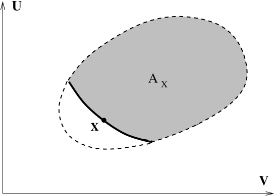
Figure 2. The coordinates $U$ and $V$ of a simple system. The state space (bounded by dashed line) and the forward sector $A_{X}$ (shaded) of a state $X$ are convex, by axiom A7. The boundary of $A_{X}$ (full line) is an adiabat, cf. Theorem 3.

We need three more axioms for simple systems, which will take us into an analytic detour. The first of these establishes (a) above.

1. Irreversibility. For each $X\in\Gamma$ there is a point $Y\in\Gamma$ such that $X\prec\prec Y$. (This axiom is implied by A14 below, but is stated here separately because important conclusions can be drawn from it alone.)

2. Lipschitz tangent planes. For each $X\in\Gamma$ the forward sector $A_{X}=\{Y\in\Gamma:X\prec Y\}$ has a unique support plane at $X$ (i.e., $A_{X}$ has a tangent plane at $X$). The tangent plane is assumed to be a locally Lipschitz continuous function of $X$, in the sense explained below.

3. Connectedness of the boundary. The boundary $\partial A_{X}$ (relative to the open set $\Gamma$) of every forward sector $A_{X}\subset\Gamma$ is connected. (This is technical and conceivably can be replaced by something else.)

Axiom A8 plus Lemma 1 asserts that every $X$ lies on the boundary $\partial A_{X}$ of its forward sector. Although axiom A9 asserts that the convex set, $A_{X}$, has a true tangent at $X$ only, it is an easy consequence of axiom A2 that $A_{X}$ has a true tangent everywhere on its boundary. To say that this tangent plane is locally Lipschitz continuous means that if $X=(U^{0},V^{0})$ then this plane is given by

$$U-U^{0}+\sum^{n}_{1}P_{i}(X)(V_{i}-V^{0}_{i})=0\,.$$ (34)

with locally Lipschitz continuous functions $P_{i}$. The function $P_{i}$ is called the generalized pressure conjugate to the work coordinate $V_{i}$ . (When $V_{i}$ is the volume, $P_{i}$ is the ordinary pressure.)

Lipschitz continuity and connectedness is a well known guarantee for uniqueness of the solution to the coupled differential equations

$$\tfrac{\partial u}{\partial V_{j}}(V)=-P_{j}\big{(}u(V),V\big{)}\quad{\rm for}\ j=1,\dots,n$$ (35)

which describes the boundary $\partial A_{X}$ of $A_{X}$.

With these axioms one can now prove that the comparison hypothesis holds for the state space $\Gamma$ of a simple system:

Theorem 3 (CH for simple systems).

If $X$ and $Y$ are states of the same simple system, then either $X\prec Y$ or $Y\prec X$. Moreover, $X\mathrel{\overset{\rm\scriptscriptstyle A}{\sim}}Y\Longleftrightarrow Y\in\partial A_{X}\Longleftrightarrow X\in\partial A_{Y}$.

Proof.

The proof is carried out in several steps, which provide also further information about the forward sectors.

Step 1: $A_{X}$ is closed. We have to prove that if $Y\in\Gamma$ is on the boundary of $A_{X}$ then $Y$ is in $A_{X}$. For this purpose we can assume that the set $A_{X}$ has full dimension, i.e., the interior of $A_{X}$ is not empty. If, on the contrary, $A_{X}$ lay in some lower dimensional hyperplane then the following proof would work, without any changes, simply by replacing $\Gamma$ by the intersection of $\Gamma$ with this hyperplane.

Let $W$ be any point in the interior of $A_{X}$. Since $A_{X}$ is convex, and $Y$ is on the boundary of $A_{X}$, the half-open line segment joining $W$ to $Y$ (call it $[W,Y)$, bearing in mind that $Y\not\in[W,Y)$) lies in $A_{X}$. The prolongation of this line beyond $Y$ lies in the complement of $A_{X}$ and has at least one point (call it $Z$) in $\Gamma$. (This follows from the fact that $\Gamma$ is open and $Y\in\Gamma$.) For all sufficiently large integers $n$ the point $Y_{n}$ defined by

$$\hbox{${\frac{n}{n+1}}$}Y_{n}+\hbox{${\frac{1}{n+1}}$}Z=Y$$ (36)

belongs to $[W,Y)$. We claim that $(X,\hbox{${\frac{1}{n}}$}Z)\prec(Y,\hbox{${\frac{1}{n}}$}Y)$. If this is so then we are done because, by the stability axiom, A6, $X\prec Y$.

To prove the last claim, first note that $(X,\hbox{${\frac{1}{n}}$}Z)\prec(Y_{n},\hbox{${\frac{1}{n}}$}Z)$ because $X\prec Y_{n}$ and by axiom A3. By scaling, A4, the convex combination axiom A7, and (3.10)

$$\left(Y_{n},\hbox{${\frac{1}{n}}$}Z\right)\ =\hbox{${\frac{{n+1}}{n}}$}\left(\hbox{${\frac{n}{n+1}}$}Y_{n},\hbox{${\frac{1}{n+1}}$}Z\right)\ \prec\ \hbox{${\frac{n+1}{n}}$}Y\ .$$ (37)

But this last equals $(Y,\frac{1}{n}Y)$ by the splitting axiom, A5. Hence $(X,\frac{1}{n}Z)\prec(Y,\frac{1}{n}Y)$.

Step 2: $A_{X}$ has a nonempty interior. $A_{X}$ is a convex set by axiom A7. Hence, if $A_{X}$ had an empty interior it would necessarily be contained in a hyperplane. [An illustrative picture to keep in mind here is that $A_{X}$ is a closed, (two-dimensional) disc in ${\mathbb{R}}^{3}$ and $X$ is some point inside this disc and not on its perimeter. This disc is a closed subset of ${\mathbb{R}}^{3}$ and $X$ is on its boundary (when the disc is viewed as a subset of ${\mathbb{R}}^{3}$). The hyperplane is the plane in ${\mathbb{R}}^{3}$ that contains the disc.]

Any hyperplane containing $A_{X}$ is a support plane to $A_{X}$ at $X$, and by axiom A9 the support plane, $\Pi_{X}$, is unique, so $A_{X}\subset\Pi_{X}$. If $Y\in A_{X}$, then $A_{Y}\subset A_{X}\subset\Pi_{X}$ by transitivity, A2. By the irreversibility axiom A8, there exists a $Y\in A_{X}$ such that $A_{Y}\neq A_{X}$, which implies that the convex set $A_{Y}\subset\Pi_{X}$, regarded as a subset of $\Pi_{X}$, has a boundary point in $\Pi_{X}$. If $Z\in\Pi_{X}$ is such a boundary point of $A_{Y}$, then $Z\in A_{Y}$ because $A_{Y}$ is closed. By transitivity, $A_{Z}\subset A_{Y}\subset\Pi_{X}$, and $A_{Z}\neq\Pi_{X}$ because $A_{Y}\neq A_{X}$.

Now $A_{Y}$, considered as a subset of $\Pi_{X}$, has an $(n-1)$-dimensional supporting hyperplane at $Z$ (because $Z$ is a boundary point). Call this hyperplane $\Pi^{\prime}_{Z}$. Since $A_{Z}\subset A_{Y}$, $\Pi_{Z}^{\prime}$ is a supporting hyperplane for $A_{Z}$, regarded as a subset of $\Pi_{X}$. Any $n$-dimensional hyperplane in ${\mathbb{R}}^{n+1}$ that contains the $(n-1)$-dimensional hyperplane $\Pi^{\prime}_{Z}\subset\Pi_{X}$ clearly supports $A_{Z}$ at $Z$, where $A_{Z}$ is now considered as a convex subset of ${\mathbb{R}}^{n+1}$. Since there are infinitely many such $n$-dimensional hyperplanes in ${\mathbb{R}}^{n+1}$, we have a contradiction to the uniqueness axiom A9.

Step 3: $Y\in\partial A_{X}$ $\Rightarrow$ $X\in\partial A_{Y}$ and hence $A_{X}=A_{Y}$. We bring here only a sketch of the proof; for details see [LY1], Theorems 3.5 and 3.6. First, using the convexity axiom, A7, and the existence of a tangent plane of $A_{X}$ at $X$, one shows that the boundary points of $A_{X}$ can be written as $(u_{X}(V),V)$, where $u_{X}$ is a solution to the equation system (35). Here $V$ runs through the set

$$\rho_{X}=\{V:\ (U,V)\in\partial A_{X}\ \text{for some}\ U\}.$$ (38)

Secondly, the solution of (35) that passes through $X$ is unique by the Lipschitz condition for the pressure. In particular, if $Y\in\partial A_{X}$, then $u_{X}$ must coincide on $\rho_{Y}\subset\rho_{X}$ with the solution $u_{Y}$ through $Y$. The proof is completed by showing that $\rho_{X}=\rho_{Y}$; this uses that $\rho_{X}$ is connected by axiom A10 and also that $\rho_{X}$ is open. For the latter it is important that no tangent plane of $A_{X}$ can be parallel to the $U$-axis, because of axiom A9.

Step 4: $X\notin A_{Y}$ $\Rightarrow$ $Y\in A_{X}$. Let $Z$ be some point in the interior of $A_{Y}$ and consider the line segment $L$ joining $X$ to $Z$. If we assume $X\notin A_{Y}$ then part of $L$ lies outside $A_{Y}$, and therefore $L$ intersects $\partial A_{Y}$ at some point $W\in\partial A_{Y}$. By Step 3, $A_{Y}$ and $A_{W}$ are the same set, so $W\prec Z$ (because $Y\prec Z$). We claim that this implies $X\prec Z$ also. This can be seen as follows:

We have $W=tX+(1-t)Z$ for some $t\in(0,1)$. By A7, A5, $W\prec Z$, and A3

$$(tX,(1-t)Z)\prec W\mathrel{\overset{\rm\scriptscriptstyle A}{\sim}}(tW,(1-t)W)\prec(tW,(1-t)Z).$$ (39)

By transitivity, A2, and the cancellation law, (5), $tX\prec tW$. By scaling, A4, $X\prec W$ and hence, by A2, $X\prec Z$.

Since $Z$ was arbitrary, we learn that ${\rm Interior}(A_{Y})\subset A_{X}$. Since $A_{X}$ and $A_{Y}$ are both closed by Step 1, this implies $A_{Y}\subset A_{X}$ and hence, by A1, $Y\in A_{X}$.

Step 5: $X\mathrel{\overset{\rm\scriptscriptstyle A}{\sim}}Y$ $\Longleftrightarrow$ $Y\in\partial A_{X}$. By Step 1, $A_{X}$ is closed, so $\partial A_{X}\subset A_{X}$. Hence, if $Y\in\partial A_{X}$, then $X\prec Y$. By Step 3, $Y\in\partial A_{X}$ is equivalent to $X\in\partial A_{Y}$, so we can also conclude that $Y\prec X$. The implication $\Longleftarrow$ is thus clear. On the other hand, $X\mathrel{\overset{\rm\scriptscriptstyle A}{\sim}}Y$ implies $A_{X}=A_{Y}$ by Axiom A2 and thus $\partial A_{X}=\partial A_{Y}$. But $Y\in\partial A_{Y}$ by Axioms A1, A8 and Lemma 1. Thus the adiabats, i.e., the $\mathrel{\overset{\rm\scriptscriptstyle A}{\sim}}$ equivalence classes, are exactly the boundaries of the forward sectors. ∎

Figure 3. This figure illustrates Theorem 3, i.e., the fact that forward sectors of a simple system are nested. The bottom figure shows what could, in principle, go wrong—but does not.

Remark.

It can also be shown from our axioms that the orientation of forward sectors w.r.t. the energy axis is the same for all simple systems (cf. [LY1], Thms. 3.3 and 4.2). By convention we choose the direction of the energy axis so that the the energy always increases in adiabatic processes at fixed work coordinates. When temperature is defined later, this will imply that temperature is always positive. Since spin systems in magnetic fields are sometimes regarded as capable of having ‘negative temperatures’ it is natural to ask what in our axioms excludes such situations. The answer is: Convexity, A7, together with axiom A8. The first would imply that if the energy can both increase and decrease in adiabatic processes, then also a state of maximal energy is in the state space. But such a state would also have maximal entropy and thus violate A8. From our point of view, ‘negative temperature’ states should not be regarded as true equilibrium states.

Before leaving the subject of simple systems let us remark on the connection with Carathéodory’s development. The point of contact is the fact that $X\in\partial A_{X}$. We assume that $A_{X}$ is convex and use transitivity and Lipschitz continuity to arrive, eventually, at Theorem 3. Carathéodory uses Frobenius’s theorem, plus assumptions about differentiability to conclude the existence – locally – of a surface containing $X$. Important global information, such as Theorem 3, are then not easy to obtain without further assumptions, as discussed, e.g., in [B].

The next topic is thermal contact and the zeroth law, which entails the very special assumptions about $\prec$ that we mentioned earlier. It will enable us to establish CH for products of several systems, and thereby show, via Theorem 2, that entropy exists and is additive. Although we have established CH for a simple system, $\Gamma$, we have not yet established CH even for a product of two copies of $\Gamma$. This is needed in the definition of $S$ given in (9). The $S$ in (9) is determined up to an affine shift and we want to be able to calibrate the entropies (i.e., adjust the multiplicative and additive constants) of all systems so that they work together to form a global $S$ satisfying the entropy principle. We need five more axioms. They might look a bit abstract, so a few words of introduction might be helpful.

In order to relate systems to each other, in the hope of establishing CH for compounds, and thereby an additive entropy function, some way must be found to put them into contact with each other. Heuristically, we imagine two simple systems (the same or different) side by side, and fix the work coordinates (e.g., the volume) of each. Bring them into ‘thermal contact’ (e.g., by linking them to each other with a copper thread) and wait for equilibrium to be established. The total energy $U$ will not change but the individual energies, $U_{1}$ and $U_{2}$ will adjust to values that depend on $U$ and the work coordinates. This new system (with the thread permanently connected) then behaves like a simple system (with one energy coordinate) but with several work coordinates (the union of the two work coordinates). Thus, if we start initially with $X=(U_{1},V_{1})$ for system 1 and $Y=(U_{2},V_{2})$ for system 2, and if we end up with $Z=(U,V_{1},V_{2})$ for the new system, we can say that $(X,Y)\prec Z$. This holds for every choice of $U_{1}$ and $U_{2}$ whose sum is $U$. Moreover, after thermal equilibrium is reached, the two systems can be disconnected, if we wish, and once more form a compound system, whose component parts we say are in thermal equilibrium. That this is transitive is the zeroth law.

Thus, we cannot only make compound systems consisting of independent subsystems (which can interact, but separate again), we can also make a new simple system out of two simple systems. To do this an energy coordinate has to disappear, and thermal contact does this for us. This is formalized in the following two axioms.

1. Thermal join. For any two simple systems with state-spaces $\Gamma_{1}$ and $\Gamma_{2}$, there is another simple system, called the thermal join of $\Gamma_{1}$ and $\Gamma_{2}$, with state-space

   $$\Delta_{12}=\big{\{}(U,V_{1},V_{2}):U=U_{1}+U_{2}\;{\rm with}\;(U_{1},V_{1})\in\Gamma_{1}\,,\ (U_{2},V_{2})\in\Gamma_{2}\big{\}}\,.$$ (40)

   If $X=(U_{1},V_{1})\in\Gamma_{1}$, and $Y=(U_{2},V_{2})\in\Gamma_{2}$ we define

   $$\theta(X,Y):=(U_{1}+U_{2},V_{1},V_{2})\in\Delta_{12}.$$ (41)

   It is assumed that the formation of a thermal join is an adiabatic operation for the compound system, i.e.,

   $$(X,Y)\prec\theta(X,Y).$$ (42)

2. Thermal splitting. For any point $Z\in\Delta_{12}$ there is at least one pair of states, $X\in\Gamma_{1}$, $Y\in\Gamma_{2}$, such that

   $$Z=\theta(X,Y)\mathrel{\overset{\rm\scriptscriptstyle A}{\sim}}(X,Y)$$ (43)

Definition. If $\theta(X,Y)\mathrel{\overset{\rm\scriptscriptstyle A}{\sim}}(X,Y)$ we say that the states $X$ and $Y$ are in thermal equilibrium and write

$$X\mathrel{\overset{\rm\scriptscriptstyle T}{\sim}}Y\,.$$ (44)

A11 and A12 together say that for each choice of the individual work coordinates there is a way to divide up the energy $U$ between the two systems in a stable manner. A12 is the stability statement, for it says that joining is reversible, i.e., once the equilibrium has been established, one can cut the copper thread and retrieve the two systems back again, but with a special partition of the energies. This reversibility allows us to think of the thermal join, which is a simple system in its own right, as a special subset of the product system, $\Gamma_{1}\times\Gamma_{2}$, which we call the thermal diagonal.

Axioms A11 and A12, together with the general axioms A4, A5, A7 and our assumption that a compound state $(X,Y)$ is identical to $(Y,X)$, imply that the relation $\mathrel{\overset{\rm\scriptscriptstyle T}{\sim}}$ is refelxive and symmetric:

lemma 2 .

1. $X\mathrel{\overset{\rm\scriptscriptstyle T}{\sim}}X$.

2. If $X\mathrel{\overset{\rm\scriptscriptstyle T}{\sim}}Y$, then $Y\mathrel{\overset{\rm\scriptscriptstyle T}{\sim}}X$.

Proof.

(i) Let $X=(U,V)$. Then, by A11,

$$(X,X)\prec\theta(X,X)=(2U,V,V).$$ (45)

By A12, this is, for some $U^{\prime}$ and $U^{\prime\prime}$ with $U^{\prime}+U^{\prime\prime}=2U$,

$$\mathrel{\overset{\rm\scriptscriptstyle A}{\sim}}((U^{\prime},V),(U^{\prime\prime},V)),$$ (46)

which, using A4, A7, and finally A5, is

$$\mathrel{\overset{\rm\scriptscriptstyle A}{\sim}}2(\hbox{${\frac{1}{2}}$}(U^{\prime},V),\hbox{${\frac{1}{2}}$}(U^{\prime\prime},V))\prec 2(\hbox{${\frac{1}{2}}$}(U^{\prime}+U^{\prime\prime}),V)=2X\mathrel{\overset{\rm\scriptscriptstyle A}{\sim}}(X,X).$$ (47)

Hence $(X,X)\mathrel{\overset{\rm\scriptscriptstyle A}{\sim}}\theta(X,X)$, i.e., $X\mathrel{\overset{\rm\scriptscriptstyle T}{\sim}}X$.

(ii) By A11 and A12 we have quite generally

$$\theta(X,Y)=(U_{X}+U_{Y},V_{X},V_{Y})\mathrel{\overset{\rm\scriptscriptstyle A}{\sim}}((U^{\prime},V_{X}),(U^{\prime\prime},V_{Y}))$$ (48)

for some $U^{\prime}$, $U^{\prime\prime}$ with $U^{\prime}+U^{\prime\prime}=U_{X}+U_{Y}=U_{Y}+U_{X}$. Since composition of states is commutative (i.e., $(A,B)=(B,A)$, as we stated when explaining the basic concepts) we obtain, using A11 again,

$$((U^{\prime},V_{X}),(U^{\prime\prime},V_{Y}))=((U^{\prime\prime},V_{Y}),(U^{\prime},V_{X}))\prec(U^{\prime\prime}+U^{\prime},V_{Y},V_{X})=\theta(Y,X).$$ (49)

Interchanging $X$ and $Y$ we thus have $\theta(X,Y)\mathrel{\overset{\rm\scriptscriptstyle A}{\sim}}\theta(Y,X)$. Hence, if $X\mathrel{\overset{\rm\scriptscriptstyle T}{\sim}}Y$, i.e., $(X,Y)\mathrel{\overset{\rm\scriptscriptstyle A}{\sim}}\theta(X,Y)$, then $(Y,X)=(X,Y)\mathrel{\overset{\rm\scriptscriptstyle A}{\sim}}\theta(X,Y)\mathrel{\overset{\rm\scriptscriptstyle A}{\sim}}\theta(Y,X)$, i.e., $Y\mathrel{\overset{\rm\scriptscriptstyle T}{\sim}}X$. ∎

Remark.

Instead of presenting a formal proof of the symmetry of $\mathrel{\overset{\rm\scriptscriptstyle T}{\sim}}$, it might seem more natural to simply identify $\theta(X,Y)$ with $\theta(Y,X)$ by an additional axiom. This could be justified both from the physical interpretation of the thermal join, which is symmetric in the states (connect the systems with a copper thread), and also because both joins have the same energy and the same work coordinates, only written in different order. But since we really only need that $\theta(X,Y)\mathrel{\overset{\rm\scriptscriptstyle A}{\sim}}\theta(Y,X)$ and this follows from the axioms as they stand, it is not necessary to postulate such an identification. Likewise, it is not necessary to identify $\theta(\theta(X,Y),Z)$ with $\theta(X,\theta(Y,Z))$ formally by an axiom, because we do not need it. It is possible, using the present axioms, to prove $\theta(\theta(X,Y),Z)\mathrel{\overset{\rm\scriptscriptstyle A}{\sim}}\theta(X,\theta(Y,Z))$, but we do not do so since we do not need this either.

We now come to the famous zeroth law, which says that the thermal equilibrium is transitive, and hence (by Lemma 2) an equivalence relation.

1. Zeroth law of thermodynamics. If $X\mathrel{\overset{\rm\scriptscriptstyle T}{\sim}}Z$ and $Z\mathrel{\overset{\rm\scriptscriptstyle T}{\sim}}Y$ then $X\mathrel{\overset{\rm\scriptscriptstyle T}{\sim}}Y$.

The zeroth law is often taken to mean that the equivalence classes can be labeled by an ‘empirical’ temperature, but we do not want to mention temperature at all at this point. It will appear later.

There are two more axioms about thermal contact, but before we state them we draw two simple conclusions from A11, A12 and A13.

lemma 3.

1. If $X\mathrel{\overset{\rm\scriptscriptstyle T}{\sim}}Y$, then $\lambda X\mathrel{\overset{\rm\scriptscriptstyle T}{\sim}}\mu Y$ for all $\lambda,\mu>0$.

2. If $X\mathrel{\overset{\rm\scriptscriptstyle T}{\sim}}Y$ and $Z\mathrel{\overset{\rm\scriptscriptstyle T}{\sim}}X$, then $Z\mathrel{\overset{\rm\scriptscriptstyle T}{\sim}}\theta(X,Y)$.

Proof.

(i) By the zeroth law, A13, it suffices to show that $\lambda X\mathrel{\overset{\rm\scriptscriptstyle T}{\sim}}X$ and $\mu Y\mathrel{\overset{\rm\scriptscriptstyle T}{\sim}}Y$. For this we use similar arguments as in Lemma 2(i):

$$(\lambda X,X)\prec\theta(\lambda X,X)=((1+\lambda)U,\lambda V,V)\mathrel{\overset{\rm\scriptscriptstyle A}{\sim}}((\lambda U^{\prime},\lambda V),(U^{\prime\prime},V))$$ (50)

with $\lambda U^{\prime}+U^{\prime\prime}=(1+\lambda)U$. By A4, A7, and A5 this is

$$\mathrel{\overset{\rm\scriptscriptstyle A}{\sim}}(1+\lambda)(\hbox{${\frac{\lambda}{1+\lambda}}$}(U^{\prime},V),\hbox{${\frac{1}{1+\lambda}}$}(U^{\prime\prime},V))\prec(1+\lambda)(\hbox{${\frac{1}{1+\lambda}}$}(\lambda U^{\prime}+U^{\prime\prime}),V)=(1+\lambda)X\mathrel{\overset{\rm\scriptscriptstyle A}{\sim}}(\lambda X,X).$$ (51)

(ii) By the zeroth law, it suffices to show that $X\mathrel{\overset{\rm\scriptscriptstyle T}{\sim}}\theta(X,Y)$, i.e.,

$$(X,\theta(X,Y))\mathrel{\overset{\rm\scriptscriptstyle A}{\sim}}\theta(X,\theta(X,Y)).$$ (52)

The left side of this equation is $\prec$ the right side by A11, so we need only show

$$\theta(X,\theta(X,Y))\prec(X,\theta(X,Y)).$$ (53)

Now, since $X\mathrel{\overset{\rm\scriptscriptstyle T}{\sim}}Y$ and hence also $2X\mathrel{\overset{\rm\scriptscriptstyle T}{\sim}}Y$ by (i), the right side of (53) is

$$(X,\theta(X,Y))\mathrel{\overset{\rm\scriptscriptstyle A}{\sim}}(X,(X,Y))=((X,X),Y)\mathrel{\overset{\rm\scriptscriptstyle A}{\sim}}(2X,Y)\mathrel{\overset{\rm\scriptscriptstyle A}{\sim}}\theta(2X,Y)=(2U_{X}+U_{Y},2V_{X},V_{Y}).$$ (54)

(Here A5, A4 and A3 have been used, besides (i)). On the other hand, using A12 twice as well as A3, we have for some $X^{\prime}=(U^{\prime},V_{X})$, $X^{\prime\prime}=(U^{\prime\prime},V_{X})$ and $Y^{\prime}=(U^{\prime\prime\prime},V_{Y})$ with $U^{\prime}+U^{\prime\prime}+U^{\prime\prime\prime}=2U_{X}+U_{Y}$:

$$\theta(X,\theta(X,Y))\mathrel{\overset{\rm\scriptscriptstyle A}{\sim}}(X^{\prime},(X^{\prime\prime},Y^{\prime}))=((X^{\prime},X^{\prime\prime}),Y^{\prime})\ .$$ (55)

By convexity A7 and scaling A4, as above, this is

$$\prec(X^{\prime}+X^{\prime\prime},Y^{\prime})\prec\theta(X^{\prime}+X^{\prime\prime},Y^{\prime})=(2U_{X}+U_{Y},2V_{X},V_{Y}).$$ (56)

But this is $\mathrel{\overset{\rm\scriptscriptstyle A}{\sim}}(X,\theta(X,Y))$ by (54). ∎

We now turn to the remaining two axioms about thermal contact.

A14 requires that for every adiabat (i.e., an equivalence class w.r.t. $\mathrel{\overset{\rm\scriptscriptstyle A}{\sim}}$) there exists at least one isotherm (i.e., an equivalence class w.r.t. $\mathrel{\overset{\rm\scriptscriptstyle T}{\sim}}$), containing points on both sides of the adiabat. Note that, for each given $X$, only two points in the entire state space $\Gamma$ are required to have the stated property. This assumption essentially prevents a state-space from breaking up into two pieces that do not communicate with each other. Without it, counterexamples to CH for compound systems can be constructed, cf. [LY1], Section 4.3. A14 implies A8, but we listed A8 separately in order not to confuse the discussion of simple systems with thermal equilibrium.

A15 is a technical and perhaps can be eliminated. Its physical motivation is that a sufficiently large copy of a system can act as a heat bath for other systems. When temperature is introduced later, A15 will have the meaning that all systems have the same temperature range. This postulate is needed if we want to be able to bring every system into thermal equilibrium with every other system.

1. Transversality. If $\Gamma$ is the state space of a simple system and if $X\in\Gamma$, then there exist states $X_{0}\mathrel{\overset{\rm\scriptscriptstyle T}{\sim}}X_{1}$ with $X_{0}\prec\prec X\prec\prec X_{1}$.

2. Universal temperature range. If $\Gamma_{1}$ and $\Gamma_{2}$ are state spaces of simple systems then, for every $X\in\Gamma_{1}$ and every $V$ belonging to the projection of $\Gamma_{2}$ onto the space of its work coordinates, there is a $Y\in\Gamma_{2}$ with work coordinates $V$ such that $X\mathrel{\overset{\rm\scriptscriptstyle T}{\sim}}Y$.

Figure 4. Transversality, A14, requires that on on each side of the adiabat through any point $X$ there are points, $X_{0}$ and $X_{1}$, that are in thermal equilibrium with each other.

The reader should note that the concept ‘thermal contact’ has appeared, but not temperature or hot and cold or anything resembling the Clausius or Kelvin-Planck formulations of the second law. Nevertheless, we come to the main achievement of our approach: With these axioms we can establish CH for products of simple systems (each of which satisfies CH, as we already know). The proof has two parts. In the first, we consider multiple scaled copies of the same simple system and use the thermal join and in particular transversality to reduce the problem to comparability within a single simple system, which is already known to hold by Theorem 3. The basic idea here is that with $X,X_{0},X_{1}$ as in A14, the states $((1-\lambda)X_{0},\lambda X_{1})$ and $((1-\lambda)X,\lambda X)$ can be regarded as states of the same simple system and are, therefore, comparable. This is the key point needed for the construction of $S$, according to $(9)$. The importance of transversality is thus brought into focus. In the second part we consider products of different simple systems. This case is more complicated and requires all the axioms A1–A14, in particular the zeroth law, A13.

lemma 4 (CH in multiple scaled copies of a simple system).

For any simple system $\Gamma$, all states of the form $(\lambda_{1}Y_{1},\lambda_{2}Y_{2}\dots)$ with $Y_{i}\in\Gamma$ and $\sum_{i}\lambda_{i}$ fixed are comparable.

Proof.

By scaling invariance of the relation $\prec$ (Axiom A4) we may assume that $\sum_{i}\lambda_{i}=1$. Now suppose $Y_{1},\dots,Y_{N},Y_{1}^{\prime},\dots,Y_{M}^{\prime}\in\Gamma$, and $\lambda_{1},\dots,\lambda_{N},\lambda_{1}^{\prime},\dots,\lambda_{M}^{\prime}\in{\mathbb{R}}$ with $\sum_{i}\lambda_{i}=\sum_{j}\lambda_{j}^{\prime}=1$. We shall show that for some $\bar{X}_{0},\bar{X}_{1}\in\Gamma$ with $\bar{X}_{0}\prec\prec\bar{X}_{1}$ and some $\lambda,\lambda^{\prime}\in{\mathbb{R}}$

$$(\lambda_{1}Y_{1},\dots,\lambda_{N}Y_{N}) \mathrel{\overset{\rm\scriptscriptstyle A}{\sim}} ((1-\lambda)\bar{X}_{0},\lambda\bar{X}_{1}),$$ (57)

$$(\lambda_{1}^{\prime}Y_{1}^{\prime},\dots,\lambda_{M}^{\prime}Y_{M}^{\prime}) \mathrel{\overset{\rm\scriptscriptstyle A}{\sim}} ((1-\lambda^{\prime})\bar{X}_{0},\lambda^{\prime}\bar{X}_{1}).$$ (58)

This will prove the lemma, since we already know from the equivalence of (11) and (12) that the right sides of (57) and (58) are comparable.

It was already noted that if $X_{0}\prec\prec X_{1}$ and $X_{0}\mathrel{\overset{\rm\scriptscriptstyle T}{\sim}}X_{1}$, then every $X$ in the ‘strip’ $\Sigma(X_{0},X_{1}):=\{X:\ X_{0}\prec X\prec X_{1}\}$ is comparable to $((1-\lambda)X_{0},\lambda X_{1})$ for any $0\leq\lambda\leq 1$, due to the axioms A5, A11, A12, and Theorem 3. This implies in the same way as in the proof of Theorem 1 that $X$ is in fact adiabatically equivalent to $((1-\lambda)X_{0},\lambda X_{1})$ for some $\lambda$. (Namely, $\lambda=\lambda_{\rm max}$, defined by (13).) Moreover, if each of the points $Y_{1},Y_{2}\dots,Y^{\prime}_{M-1},Y^{\prime}_{M}$ is adiabatically equivalent to such a combination of a common pair of points $\bar{X}_{0}\prec\prec\bar{X}_{1}$ (which need not be in thermal equilibrium), then Eqs. (57) and (58) follow easily from the recombination axiom A5. The existence of such a common pair of reference points is proved by the following stepwise extension of ‘local’ strips defined by points in thermal equilibrium.

By the transversality property, A4, the whole state space $\Gamma$ can be covered by strips $\sum(X^{(i)}_{0},X^{(i)}_{1})$ with $X^{(i)}_{0}\prec\prec X^{(i)}_{0}$ and $X^{(i)}_{0}\mathrel{\overset{\rm\scriptscriptstyle T}{\sim}}X^{(i)}_{1}$. Here $i$ belongs to some index set. Since all adiabats $\partial A_{X}$ with $X\in\Gamma$ are relatively closed in $\Gamma$ we can even cover each $X$ (and hence $\Gamma$) with the open strips $\mathop{{\sum}_{i}}\limits^{o}:=\sum\limits^{o}(X^{(i)}_{0},X^{(i)}_{1})=\{X:X^{(i)}_{0}\prec\prec X\prec\prec X^{(i)}_{0}\}$. Moreover, any compact subset, $C$, of $\Gamma$ is covered by a finite number of such strips $\mathop{{\sum}_{i}}\limits^{o},i=1,\dots,K$, and if $C$ is connected we may assume that $\mathop{{\sum}_{i}}\limits^{o}\cap\mathop{{\sum}_{i+1}}\limits^{o{\phantom{111}}}\not=\emptyset$. In particular, this holds if $C$ is some polygonal path connecting the points $Y_{1},\dots,Y_{N},Y_{1}^{\prime},\dots,Y_{M}^{\prime}$.

By Theorem 3, the points $X^{(1)}_{0},X^{(1)}_{1}\dots X^{(K)}_{0},X^{(K)}_{1}$, can be ordered according to the relation $\prec$, and there is no restriction to assume that

$$X^{(i)}_{0}\prec\prec X^{(i+1)}_{0}\prec\prec X^{(i)}_{1}\prec\prec X^{(i+1)}_{1}.$$ (59)

Let $\bar{X}_{0}=X^{(1)}_{0}$ denote the ‘smallest’ and $\bar{X}_{1}=X^{(K)}_{1}$ the ‘largest’ of these points. We claim that every one of the points $Y_{1},\dots,Y_{N},Y_{1}^{\prime},\dots,Y_{M}^{\prime}$ is adiabatically equivalent to a combination of $\bar{X}_{0}$ and $\bar{X}_{1}$. This is based on the following general fact:

Suppose $X_{0}\prec\prec X_{1},\,X^{\prime}_{0}\prec\prec X^{\prime}_{1}$ and

$$X_{1}\mathrel{\overset{\rm\scriptscriptstyle A}{\sim}}((1-\lambda_{1})X^{\prime}_{0},\lambda_{1}X^{\prime}_{1}),\quad\quad X^{\prime}_{0}\mathrel{\overset{\rm\scriptscriptstyle A}{\sim}}((1-\lambda_{0})X_{0},\lambda_{0}X_{1}).$$ (60)

If

$$X\mathrel{\overset{\rm\scriptscriptstyle A}{\sim}}((1-\lambda)X_{0},\lambda X_{1}),$$ (61)

then

$$X\mathrel{\overset{\rm\scriptscriptstyle A}{\sim}}((1-\mu)X_{0},\mu X^{\prime}_{1})$$ (62)

with

$$\mu=\frac{\lambda\lambda_{1}}{1-\lambda_{0}+\lambda_{0}\lambda_{1}},$$ (63)

and if

$$X\mathrel{\overset{\rm\scriptscriptstyle A}{\sim}}((1-\lambda^{\prime})X^{\prime}_{0},\lambda^{\prime}X^{\prime}_{1}),$$ (64)

then

$$X\mathrel{\overset{\rm\scriptscriptstyle A}{\sim}}((1-\mu^{\prime})X_{0},\mu^{\prime}X^{\prime}_{1})$$ (65)

with

$$\mu^{\prime}=\frac{\lambda^{\prime}(1-\lambda_{0})+\lambda_{0}\lambda_{1}}{1-\lambda_{0}+\lambda_{0}\lambda_{1}}.$$ (66)

The proof of (62) and (65) is simple arithmetics, using the splitting and recombination axiom, A5, and the cancellation law, Eq. (5). Applying this successively for $i=1,\dots,K$ with $X_{0}=X^{(1)}_{0}$, $X_{1}=X^{(i)}_{1}$, $X^{\prime}_{0}=X^{(i+1)}_{0}$, $X^{\prime}_{1}=X^{(i+1)}_{1}$, proves that any $X\in\Sigma(X^{(1)}_{0},X^{(K)}_{1})$ is adiabatically equivalent to a combination of $\bar{X}_{0}=X^{(1)}_{0}$ and $\bar{X}_{1}=X^{(K)}_{1}$. As already noted, this is precisely what is neded for (57) and (58). ∎

By Theorem 1, the last lemma establishes the existence of an entropy function $S$ within the context of one simple system $\Gamma$ and its scaled copies. Axiom A7 implies that $S$ is a concave function of $X=(U,V)\in\Gamma$, i.e.,

$$(1-\lambda)S(U,V)+\lambda S(U^{\prime},V^{\prime})\leq S((1-\lambda)U+\lambda U^{\prime},(1-\lambda)V+\lambda V^{\prime}).$$ (67)

Moreover, by A11 and A12 and the properties of entropy described in Theorem 1 (i),

$$(U,V)\mathrel{\overset{\rm\scriptscriptstyle T}{\sim}}(U^{\prime},V^{\prime})\ \Longleftrightarrow\ S(U,V)+S(U^{\prime},V^{\prime})=\max_{W}[S(W,V)+S(U+U^{\prime}-W,V^{\prime})].$$ (68)

For a given $\Gamma$ the entropy function is unique up to a mutiplicative and an additive constant which are indetermined as long as we stay within the group of scaled copies of $\Gamma$. The next task is to show that the multiplicative constants can be adjusted to give a universal entropy valid for copies of different systems, i.e. to establish the hypothesis of Theorem 2. This is based on the following.

Lemma 5 (Existence of calibrators).

If $\Gamma_{1}$ and $\Gamma_{2}$ are simple systems, then there exist states $X_{0},X_{1}\in\Gamma_{1}$ and $Y_{0},Y_{1}\in\Gamma_{2}$ such that

$$X_{0}\prec\prec X_{1}\quad\quad{\rm and}\quad\quad Y_{0}\prec\prec Y_{1}$$ (69)

and

$$(X_{0},Y_{1})\mathrel{\overset{\rm\scriptscriptstyle A}{\sim}}(X_{1},Y_{0})\,.$$ (70)

The significance of this lemma is that it allows us to fix the multiplicative constants by the condition

$$S_{1}(X_{0})+S_{2}(Y_{1})=S_{1}(X_{1})+S_{2}(Y_{0})\,.$$ (71)

Proof of Lemma 5.

The proof of this lemma is not entirely simple and it involves all the axioms A1–A15. Consider the simple system $\Delta_{12}$ obtained by thermally joining $\Gamma_{1}$ and $\Gamma_{2}$. Let $Z$ be some arbitrary point in $\Delta_{12}$ and consider the adiabat $\partial A_{Z}$. Any point in $\partial A_{Z}$ is by Axiom A12 adiabatically equivalent to some pair $(X,Y)\in\Gamma_{1}\times\Gamma_{2}$. There are now two alternatives.

• For some $Z$ there are two such pairs, $(X_{0},Y_{1})$ and $(X_{1},Y_{0})$ such that $X_{0}\prec\prec X_{1}$. Since $(X_{0},Y_{1})\mathrel{\overset{\rm\scriptscriptstyle A}{\sim}}Z\mathrel{\overset{\rm\scriptscriptstyle A}{\sim}}(X_{1},Y_{0})$, this implies $Y_{0}\prec\prec Y_{1}$ and we are done.

• $(X,Y)\mathrel{\overset{\rm\scriptscriptstyle A}{\sim}}(\bar{X},\bar{Y})$ with $X\mathrel{\overset{\rm\scriptscriptstyle T}{\sim}}Y$ and $\bar{X}\mathrel{\overset{\rm\scriptscriptstyle T}{\sim}}\bar{Y}$ always implies $X\mathrel{\overset{\rm\scriptscriptstyle A}{\sim}}\bar{X}$ (and hence also $Y\mathrel{\overset{\rm\scriptscriptstyle A}{\sim}}\bar{Y}$).

The task is thus to exclude the second alternative.

The second alternative is certainly excluded if the thermal splitting of some $Z=(U,V_{1},V_{2})$ in $\Delta_{12}$ is not unique. Indeed, if $U=U_{1}+U_{2}=\bar{U}_{1}+\bar{U}_{2}$ with $U_{1}<\bar{U}_{1}$ and $Z\mathrel{\overset{\rm\scriptscriptstyle A}{\sim}}(X,Y)\mathrel{\overset{\rm\scriptscriptstyle A}{\sim}}(\bar{X},\bar{Y})$ with $X=(U_{1},V_{1})$, $\bar{X}=(\bar{U}_{1},V_{1})$, $Y=(U_{2},V_{2})$ and $\bar{Y}=(\bar{U}_{2},V_{2})$, then $X\prec\prec\bar{X}$ and $\bar{Y}\prec\prec Y$. Hence we may assume that for every $Z=(U,V_{1},V_{2})\in\Delta_{12}$ there are unique $U_{1}$ and $U_{2}$ with $U_{1}+U_{2}=U$ and $Z\mathrel{\overset{\rm\scriptscriptstyle A}{\sim}}((U_{1},V_{1}),(U_{2},V_{2}))$.

Consider now some fixed $\bar{Z}\in\Delta_{12}$ with corresponding thermal splitting $(\bar{X},\bar{Y})$, $\bar{X}\in\Gamma_{1}$, $\bar{Y}\in\Gamma_{2}$. We shall now show that the second alternative above leads to the conclusion that all points on the adiabat $\partial A_{\bar{Z}}$ are in thermal equilibrium with each other. By the zeroth law (Axiom A13) and since the domain of work coordinates corresponding to the adiabat $\partial A_{\bar{Z}}$ is connected (by Axiom A10), it is sufficient to show this for all points with a fixed work coordinate $V_{1}$ and all points with a fixed work coordinate $V_{2}$.

The second alternative means that if $Z\in\partial A_{\bar{Z}}$ has the thermal splitting $(X,Y)$, then $X\mathrel{\overset{\rm\scriptscriptstyle A}{\sim}}\bar{X}$ and $Y\mathrel{\overset{\rm\scriptscriptstyle A}{\sim}}\bar{Y}$. For a given work coordinate $V_{1}$ there is a unique $\tilde{X}=(\tilde{U}_{1},V_{1})\in\partial A_{\bar{X}}$. (Its energy coordinate is uniquely determined as a solution of the partial differential equations for the adiabat, cf. Step 3 in the proof of Theorem 3.) Hence the thermal splitting of each points $Z$ with fixed work coordinate $V_{1}$ has the form $(\tilde{X},Y)$, and $Y\mathrel{\overset{\rm\scriptscriptstyle T}{\sim}}\tilde{X}$ for all such $Y$. By the zeroth law, all $Y$’s are in thermal equilibrium with each other (since they are in thermal equilibrium with a common $\tilde{X}$), and hence, by the zeroth law and Lemma 3, all the points $\theta(\tilde{X},Y)$ are in thermal equilibrium with each other. In the same way one shows that all points in $\partial A_{\bar{Z}}$ with fixed $V_{2}$ are in thermal equilibrium with each other.

To complete the proof we now show that if a simple system, in particular $\Delta_{12}$, contains two points that are not in thermal equilibrium with each other, then there is at least one adiabat that contains such a pair. The case that all points in $\Delta_{12}$ are in thermal equilibrium with each other can be excluded, since by A15 it would imply the same for $\Gamma_{1}$ and $\Gamma_{2}$ and thus the thermal splitting would not be unique, contrary to assumption. (Note, however, that a world where all systems are in thermal equilibrium with each other is not in conflict with our axiom system. The entropy would then be an affine fuction of $U$ and $V$ for all systems. In this case, the first alternative above would always hold.)

In our proof of the existence of an adiabat with two points not in thermal equilibrium we shall make use of the already established entropy function $S$ for the simple system $\Gamma=\Delta_{12}$ which characterizes the adiabats in $\Gamma$ and moreover has the properties (67) and (68).

The fact that $S$ characterizes the adiabats means that if ${\mathcal{R}}\subset{\mathbb{R}}$ denotes the range of $S$ on $\Gamma$ then the sets

$$E_{\sigma}=\{X\in\Gamma:S(X)=\sigma\},\qquad\sigma\in{\mathcal{R}}$$ (72)

are precisely the adiabats of $\Gamma$. Furthermore, the concavity of $S$ — and hence its continuity on the connected open set $\Gamma$ — implies that ${\mathcal{R}}$ is connected, i.e., ${\mathcal{R}}$ is an interval.

Let us assume now that for any adiabat, all points on that adiabat are in thermal equilibrium with each other. We have to show that this implies that all points in $\Gamma$ are in thermal equilibrium with each other. By the zeroth law, A3, and Lemma 2 (i), $\mathrel{\overset{\rm\scriptscriptstyle T}{\sim}}$ is an equivalence relation that divides $\Gamma$ into disjoint equivalence classes. By our assumption, each such equivalence class must be a union of adiabats, which means that the equivalence classes are represented by a family of disjoint subsets of ${\mathcal{R}}$. Thus

$${\mathcal{R}}=\bigcup\limits_{\alpha\in{\mathcal{I}}}{\mathcal{R}}_{\alpha}$$ (73)

where ${\mathcal{I}}$ is some index set, ${\mathcal{R}}_{\alpha}$ is a subset of ${\mathcal{R}}$, ${\mathcal{R}}_{\alpha}\cap{\mathcal{R}}_{\beta}=0$ for $\alpha\not=\beta$, and $E_{\sigma}\mathrel{\overset{\rm\scriptscriptstyle T}{\sim}}E_{\tau}$ if and only if $\sigma$ and $\tau$ are in some common ${\mathcal{R}}_{\alpha}$.

We will now prove that each ${\mathcal{R}}_{\alpha}$ is an open set. It is then an elementary topological fact (using the connectedness of $\Gamma$) that there can be only one non-empty ${\mathcal{R}}_{\alpha}$, i.e., all points in $\Gamma$ are in thermal equilibrium with each other and our proof will be complete.

The concavity of $S(U,V)$ with respect to $U$ for each fixed $V$ implies the existence of an upper and lower $U$-derivative at each point, which we denote by $1/T_{+}$ and $1/T_{-}$, i.e.,

$$(1/T_{\pm})(U,V)=\pm\lim\limits_{\varepsilon\searrow 0}\varepsilon^{-1}[S(U\pm\varepsilon,V)-S(U,V)].$$ (74)

Eq. (68) implies that $X\mathrel{\overset{\rm\scriptscriptstyle T}{\sim}}Y$ if and only if the closed intervals $[T_{-}(X),T_{+}(X)]$ and $[T_{-}(Y),T_{+}(Y)]$ are not disjoint. Suppose that some ${\mathcal{R}}_{\alpha}$ is not open, i.e., there is $\sigma\in{\mathcal{R}}_{\alpha}$ and either a sequence $\sigma_{1}>\sigma_{2}>\sigma_{3}\cdots$, converging to $\sigma$ or a sequence $\sigma_{1}<\sigma_{2}<\sigma_{3}<\cdots$ converging to $\sigma$ with $\sigma_{i}\not\in{\mathcal{R}}_{\alpha}$. Suppose the former (the other case is similar). Then (since $T_{\pm}$ are monotone increasing in $U$ by the concavity of $S$) we can conclude that for every $Y\in E_{\sigma_{i}}$ and every $X\in E_{\sigma}$

$$T_{-}(Y)>T_{+}(X).$$ (75)

We also note, by the monotonicity of $T_{\pm}$ in $U$, that (75) necessarily holds if $Y\in E_{\mu}$ and $\mu\geq\sigma_{i}$; hence (1) holds for all $Y\in E_{\mu}$ for any $\mu>\sigma$ (because $\sigma_{i}\searrow\sigma$). On the other hand, if $\tau\leq\sigma$

$$T_{+}(Z)\leq T_{-}(X)$$ (76)

for $Z\in E_{\tau}$ and $X\in E_{\sigma}$. This contradicts transversality, namely the hypothesis that there is $\tau<\sigma<\mu$, $Z\in E_{\tau},Y\in E_{\mu}$ such that $[T_{-}(Z),T_{+}(Z)]\cap[T_{-}(Y),T_{+}(Y)]$ is not empty. ∎

With the aid of Lemma 5 we now arrive at our chief goal, which is CH for compound systems.

Theorem 4 (Entropy principle in products of simple systems).

The comparison hypothesis CH is valid in arbitrary compounds of simple systems. Hence, by Theorem 2, the relation $\prec$ among states in such state-spaces is characterized by an entropy function $S$. The entropy function is unique, up to an overall multiplicative constant and one additive constant for each simple system under consideration.

Proof.

Let $\Gamma_{1}$ and $\Gamma_{2}$ be simple systems and let $X_{0},X_{1}\in\Gamma_{1}$ and $Y_{0},Y_{1}\in\Gamma_{2}$ be points with the properties described in Lemma 5. By Theorem 1 we know that for every $X\in\Gamma_{1}$ and $Y\in\Gamma_{2}$

$$X\mathrel{\overset{\rm\scriptscriptstyle A}{\sim}}((1-\lambda_{1})X_{0},\lambda_{1}X_{1})\quad\hbox{and}\quad Y\mathrel{\overset{\rm\scriptscriptstyle A}{\sim}}((1-\lambda_{2})Y_{0},\lambda_{2}Y_{1})$$ (77)

for some $\lambda_{1}$ and $\lambda_{2}$. Define $Z_{0}=(X_{0},Y_{0})$ and $Z_{1}=(X_{1},Y_{1})$. It is then simple arithemtics, making use of (70) besides Axioms A3–A5, to show that

$$(X,Y)\mathrel{\overset{\rm\scriptscriptstyle A}{\sim}}((1-\lambda)Z_{0},\lambda Z_{1})$$ (78)

with $\lambda=\hbox{${\frac{1}{2}}$}(\lambda_{1}+\lambda_{2})$. By the equivalence of (11) and (12) we know that this is sufficient for comparability within the state space $\Gamma_{1}\times\Gamma_{2}$.

Consider now a third simple system $\Gamma_{3}$ and apply Lemma 3 to $\Delta_{12}\times\Gamma_{3}$, where $\Delta_{12}$ is the thermal join of $\Gamma_{1}$ and $\Gamma_{2}$. By Axiom A12 the reference points in $\Delta_{12}$ are adiabatically equivalent to points in $\Gamma_{1}\times\Gamma_{2}$, so we can repeat the reasoning above and conclude that all points in $(\Gamma_{1}\times\Gamma_{2})\times\Gamma_{3}$ are comparable. By induction, this extends to an arbitrary products of simple systems. This includes multiple scaled products, because by Lemma 3 and Theorem 1, every state in a multiple scaled product of copies of a simple system $\Gamma$ is adiabatically equivalent to a state in a single scaled copy of $\Gamma$. ∎

remark.

It should be emphasized that Theorem 4 contains more than the Entropy Principle for compounds of simple systems. The core of the theorem is an assertion about the comparability of all states in any state space composed of simple systems. (Note that the entropy principle would trivially be true if no state was comparable to any other state.) Combining Lemma 5 and Theorem 4 we can even assert that certain compound states in different state spaces are comparable: What counts is that the total ‘mass’ of each simple system that enters the compound is the same for both states. For instance, if $\Gamma_{1}$ and $\Gamma_{2}$ are two simple systems, and $X_{1},\dots,X_{N},X^{\prime}_{1},\dots,X^{\prime}_{N^{\prime}}\in\Gamma_{1}$, $Y_{1},\dots,Y_{M},Y^{\prime}_{1},\dots,Y^{\prime}_{M^{\prime}}\in\Gamma_{2}$, then $Z=(\lambda_{1}X_{1},\dots,\lambda_{N}X_{N},\mu_{1}Y_{1},\dots,\mu_{M}Y_{M})$ is comparable to $W=(\lambda^{\prime}_{1}X^{\prime}_{1},\dots,\lambda^{\prime}_{N^{\prime}}X^{\prime}_{N^{\prime}},\mu^{\prime}_{1}Y^{\prime}_{1},\dots,\mu^{\prime}_{M^{\prime}}Y^{\prime}_{M^{\prime}})$ provided $\sum\lambda_{i}=\sum\lambda^{\prime}_{j}$, $\sum\mu_{k}=\sum\mu^{\prime}_{\ell}$, and in this case $Z\prec W$ if and only if $S(Z)\leq S(W)$.

At last, we are now ready to define temperature. Concavity of $S$ (implied by A7), Lipschitz continuity of the pressure and the transversality condition, together with some real analysis, play key roles in the following, which answers questions Q3 and Q4 posed at the beginning.

Theorem 5 (Entropy defines temperature).

The entropy, $S$, is a concave and continuously differentiable function on the state space of a simple system. If the function $T$ is defined by

$$\tfrac{1}{T}:=\left(\tfrac{\partial S}{\partial U}\right)_{V}$$ (79)

then $T>0$ and $T$ characterizes the relation $\mathrel{\overset{\rm\scriptscriptstyle T}{\sim}}$ in the sense that $X\mathrel{\overset{\rm\scriptscriptstyle T}{\sim}}Y$ if and only if $T(X)=T(Y)$. Moreover, if two systems are brought into thermal contact with fixed work coordinates then, since the total entropy cannot decrease, the energy flows from the system with the higher $T$ to the system with the lower $T$.

Remark.

The temperature need not be a strictly monotone function of $U$; indeed, it is not so in a ‘multiphase region’ (see Fig. 5). It follows that $T$ is not always capable of specifying a state, and this fact can cause some pain in traditional discussions of the second law – if it is recognized, which usually it is not.

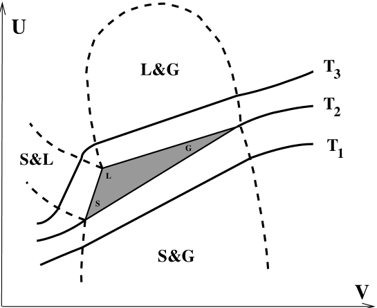
Figure 5. Isotherms in the (U,V) plane near the triple point (L=liquid, G=gas, S=solid) of a simple system. (Not to scale). In the triple point region the temperature is constant, which shows that an isotherm need not have codimension one.

Proof of Theorem 5..

The complete proof is rather long and we shall not bring all details here. They can be found in [LY1] (Lemma 5.1 and Theorems 5.1–5.4 .) As in the proof of Lemma 5, concavity of $S(U,V)$ implies the existence of the upper and lower partial derivatives of $S$ with respect to $U$ and hence of the upper and lower temperatures $T_{\pm}$ defined by (74). Moreover, as also noted in the proof of Lemma 5,

$$X\mathrel{\overset{\rm\scriptscriptstyle T}{\sim}}Y\quad\Longleftrightarrow\quad[T_{-}(X),T_{+}(X)]\cap[T_{-}(Y),T_{+}(Y)]\neq\emptyset.$$ (80)

The main goal is to show that $T_{-}=T_{+}=T$, and that $T$ is a continuous function of $X$.

Step 1: $T_{+}$ and $T_{-}$ are locally Lipschitz continuous on adiabats. The essential input here is the local Lipschitz continuity of the pressure, i.e., for each $X\in\Gamma$ and each $r>0$ there is a constant $C=C(X,r)$ such that

$$|P(X)-P(Y)|\leq C\,|X-Y|$$ (81)

if $|X-Y|<r$. The assertion is that

$$|T_{+}(X)-T_{+}(Y)|\leq c\,|X-Y|$$ (82)

for some $c=c(X,r)$, if $|X-Y|<r$ and $Y\in\partial A_{X}$, together with the analogous equation for $T_{-}$).

As in the proof of Theorem 3, Step 3, the adiabatic surface through $X=(U_{0},V_{0})$ is given by $(u_{X}(V),V)$ where $u_{X}$ is the solution to the system of differential equations

$$\frac{\partial u}{\partial V_{i}}=-P_{i},\quad i=1,\dots,n$$ (83)

with the inital condition $u(V_{0})=U_{0}$. Let us denote this solution by $u_{0}$, and consider for $\varepsilon>0$ also the solution $u_{\varepsilon}$ with the initial condition $u(V_{0})=U_{0}+\varepsilon$. This latter solution determines the adiabatic surface through $X_{\varepsilon}=(U_{0}+\varepsilon,V_{0})$ (for $V$ sufficiently close to $V_{0}$, so that $(u(V),V)\in\Gamma$).

Let $S_{0}$ denote the entropy on $(u_{0}(V),V)$ and $S_{\varepsilon}$ the entropy on $(u_{\varepsilon}(V),V)$. Then, by definition,

$$T_{+}(U_{0},V_{0})=\lim_{\varepsilon\downarrow 0}\frac{\varepsilon}{S_{\varepsilon}-S_{0}}=\lim_{\varepsilon\downarrow 0}\frac{u_{\varepsilon}(V_{0})-u_{0}(V_{0})}{S_{\varepsilon}-S_{0}}$$ (84)

and

$$T_{+}(u_{0}(V),V)=\lim_{\varepsilon\downarrow 0}\frac{u_{\varepsilon}(V)-u_{0}(V)}{S_{\varepsilon}-S_{0}}=T_{+}(U_{0},V_{0})\left[1+\lim_{\varepsilon\downarrow 0}\frac{u_{\varepsilon}(V)-u_{0}(V)-\varepsilon}{\varepsilon}\right].$$ (85)

To prove (82) it suffices to show that for all nonnegative $\varepsilon$ close to 0 and $V$ close to $V_{0}$

$$\frac{u_{\varepsilon}(V)-u_{0}(V)-\varepsilon}{\varepsilon}\leq D\,|V-V_{0}|.$$ (86)

for some $D$. This estimate (with $D=2C$) follows from (81), using (83) to write $u_{\varepsilon}(V)-u_{\varepsilon}(V_{0})$ and $u_{0}(V)-u_{0}(_{0})$ as line integrals of the pressure. See [LY1], p. 69.

Step 2: $T_{+}(X)>T_{-}(X)\,\Rightarrow\,T_{+}$ and $T_{-}$ are constant on $\partial A_{X}$. This step relies on concavity of entropy, continuity of $T_{\pm}$ on adiabats (Step 1), and last but not least, on the zeroth law. Without the zeroth law it is easy to give counterexamples to the assertion.

If $T_{+}(X)>T_{-}(X)$, but $T_{+}$ is not constant, then by continuity of $T_{\pm}$ on adiabats there exist $Y,Z$ with $Y\mathrel{\overset{\rm\scriptscriptstyle A}{\sim}}Z\mathrel{\overset{\rm\scriptscriptstyle A}{\sim}}X$, $T_{+}(Y)<T_{+}(Z)$ but $[T_{-}(Y),T_{+}(Y)]\cap[T_{-}(Z),T_{+}(Z)]\neq\emptyset$, i.e., $Y\mathrel{\overset{\rm\scriptscriptstyle T}{\sim}}Z$. Now it is a general fact about a concave function, in particular $U\mapsto S(U,V)$, that the set of points where it is differentiable, i.e., where $T_{+}(U,V)=T_{-}(U,V)\equiv T(U,V)$, is dense. Moreover, if $U_{1}>U_{2}>\dots$ is a sequence of such points converging to $U$, then $T(U_{i},V)$ converges to $T_{+}(U,V)$. Using continuity of $T_{+}$ on the adiabat, we conclude that there exists a $W$ such that $T_{+}(W)=T_{-}(W)=T(W)$, but $T_{+}(Y)<T(W)<T_{+}(Z)$. This contradicts the zeroth law, because such a $W$ would be in thermal equilibrium with $Z$ (because $T(W)\in[T_{-}(Z),T_{+}(Z)]$) but not with $Y$ (because $T(Y)\notin[T_{-}(Y),T_{+}(Y)]$). In the same way one leads the assumption that $T_{-}$ is not constant on the adiabat $\partial A_{X}$ to a contradiction.

Step 3: $T_{+}=T_{-}.$ Assume $T_{+}(X)>T_{-}(X)$ for some $X$. Then, by Step 2, $T_{+}$ and $T_{-}$ are constant on the whole adiabat $\partial A_{X}$. Now by concavity and monotonicity of $S$ in $U$ (cf. the remark following the proof of Theorem 3) we have $T_{+}(Y)\leq T_{-}(Z)$ if $S(U_{Y},V_{Y})<S(U_{Z},V_{Z})$, $V_{Y}=V_{Z}$. Hence, if $Z$ is such that

$$Y\prec\prec Z\ \hbox{and $V_{Y}=V_{Z}$ for some $Y\mathrel{\overset{\rm\scriptscriptstyle A}{\sim}}X$},$$ (87)

then $T_{+}(X)\leq T_{-}(Z)\leq T_{+}(Z)$. Likewise, if $Z^{\prime}$ is such that

$$Z^{\prime}\prec\prec Y^{\prime}\ \hbox{ and $V_{Y^{\prime}}=V_{Z^{\prime}}$ for some $Y^{\prime}\mathrel{\overset{\rm\scriptscriptstyle A}{\sim}}X$},$$ (88)

then

$$T_{-}(Z^{\prime})\leq T_{+}(Z^{\prime})\leq T_{-}(X)<T_{+}(X)\leq T_{-}(Z)\leq T_{+}(Z).$$ (89)

This means that no $Z$ satisfying (87) can be in thermal equilibrium with a $Z^{\prime}$ satisfying (88). In the case that every point in the state space has its work coordinates in common with some point on the adiabat $\partial A_{X}$, this violates the transversality axiom, A14.

Using axiom A5 we can also treat the case where the projection of the adiabat $\partial X_{X}$ onto the work coordinates, does not cover the whole range of the work coordinates for $\Gamma$, i.e., when

$$\rho_{X}:=\{V:\ (U,V)\in\partial A_{X}\ \hbox{for some}\ U\}\neq\{V:\ (U,V)\in\Gamma\ \hbox{for some}\ U\}=:\rho(\Gamma).$$ (90)

One considers a line of points $(U,\bar{V})\in\Gamma$ with $\bar{V}$ fixed on the boundary of $\rho_{X}$ in $\rho(\Gamma)$. One then shows that a gap between the upper and lower temperature of $X$, i.e., $T_{-}(X)<T_{+}(X)$, implies that points with these work coordinates $\bar{V}$ can only be in thermal equilibrium with points on one side of the adiabat $\partial A_{X}$, in contradiction to A15 and the zeroth law. See [LY1], p. 72 for the details.

Step 4: $T$ is continuous. By Step 3 $T$ is uniquely defined and by Step 1 it is locally Lipschitz continuous on each adibat, i.e.,

$$|T(X)-T(X^{\prime})|\leq c\,|X-X^{\prime}]$$ (91)

if $X\mathrel{\overset{\rm\scriptscriptstyle A}{\sim}}X^{\prime}$ and $X$ and $Y$ both lie in some ball of sufficiently small radius. Moreover, concavity of $S$ and the fact that $T_{+}=T_{-}=T$ imply that $T$ is continuous along each line $l_{V}=\{(U,V):\ (U,V)\in\Gamma\}$.

Let now $X_{\infty},X_{1},X_{2},\dots$ be points in $\Gamma$ such that $X_{j}\rightarrow X_{\infty}$ as $j\rightarrow\infty$. We write $X_{j}=(U_{j},V_{j})$, we let $A_{j}$ denote the adiabat $\partial A_{X_{j}}$, we let $T_{j}=T(X_{j})$ and we set $l_{j}=\{(U,V_{j}):(U,V_{j})\in\Gamma\}$.

By axiom A9, the slope of the tangent of $A_{X}$, i.e., the pressure $P(X)$, is locally Lipschitz continuous. Therefore for $X_{j}$ sufficiently close to $X_{\infty}$ we can assume that each adiabat $A_{j}$ intersects $l_{\infty}$ in some point, which we denote by $Y_{j}$. Since $|X_{j}-X_{\infty}|\rightarrow 0$ as $j\rightarrow\infty$, we have that $|Y_{j}\rightarrow X_{\infty}|$ as well. In particular, we can assume that all the $X_{i}$ and $Y_{j}$ lie in some small ball around $X_{\infty}$ so that (91) applies. Now

$$|T(X_{j})-T(X_{\infty})|\leq|T(X_{j})-T(Y_{j})|+|T(Y_{j})-T(X_{\infty})|,$$ (92)

and as $j\rightarrow\infty$, $T(Y_{j})-T(X_{\infty})\rightarrow 0$ because $Y_{j}$ and $X_{\infty}$ are in $l_{\infty}$. Also, $T(X_{j})-T(Y_{j})\rightarrow 0$ because $|T(X_{j})-T(Y_{j})|<c|X_{j}-Y_{j}|\leq c|X_{j}-X_{\infty}|+c|Y_{j}-X_{\infty}|$.

Step 5: $S$ is continuously differentiable. The adiabat through a point $X\in\Gamma$ is characterized by the once continuously differentiable function, $u_{X}(V)$, on ${\mathbb{R}}^{n}$. Thus, $S(u_{X}(V),V)$ is constant, so (in the sense of distributions)

$$0=\left(\frac{\partial S}{\partial U}\right)\left(\frac{\partial u_{X}}{\partial V_{j}}\right)+\frac{\partial S}{\partial V_{j}}.$$ (93)

Since $1/T=\partial S/\partial U$ is continuous, and $\partial u_{X}/\partial V_{j}=-P_{j}$ is Lipschitz continuous, we see that $\partial S/\partial V_{j}$ is a continuous function and we have the well known formula

$$\frac{\partial S}{{\partial V_{j}}}=\frac{P_{j}}{T}.$$ (94)

Step 6: Energy flows from ‘hot’ to ‘cold’. Let $X=(U_{X},V_{X})$ and $Y=(U_{Y},V_{Y})$ be two states of simple systems and assume that $T(X)>T(Y)$. By Axioms A11 and A12

$$(X,Y)\prec\theta(X,Y)\mathrel{\overset{\rm\scriptscriptstyle A}{\sim}}(X^{\prime},Y^{\prime})$$ (95)

with $X^{\prime}=(U_{X^{\prime}},V_{X})$, $Y^{\prime}=(U_{Y^{\prime}},V_{Y})$ and

$$U_{X^{\prime}}+U_{Y^{\prime}}=U_{X}+U_{Y}.$$ (96)

Moreover, $X^{\prime}\mathrel{\overset{\rm\scriptscriptstyle T}{\sim}}Y^{\prime}$ and hence, by (80) and Step 3

$$T(X^{\prime})=T(Y^{\prime})\equiv T^{*}.$$ (97)

We claim that

$$T(X)\geq T^{*}\geq T(Y).$$ (98)

(At least one of these inequalities is strict because of the uniqueness of temperature for each state.) Suppose that inequality (98) failed, e.g., $T*>T(X)>T(Y)$. Then we would have that $U_{X^{\prime}}>U_{X}$ and $U_{Y^{\prime}}>U_{Y}$ and at least one of these would be strict (by the strict monotonicity of $U$ with respect to $T$, which follows from the concavity and differentiability of $S$). This pair of inequalities is impossible in view of (96).

Since $T^{*}$ satisfies (98), the theorem now follows from the monotonicity of $U$ with respect to $T$. ∎

From the entropy principle and the relation

$$T=(\partial S/\partial U)^{-1}$$ (99)

between temperature and entropy we can now derive the usual formula for the Carnot efficiency

$$\eta_{\rm C}:=1-(T_{0}/T_{1})$$ (100)

as an upper bound for the efficiency of a ‘heat engine’ that undergoes a cyclic process. Let us define a thermal reservoir to be a simple system whose work coordinates remains unchanged during some process. Consider a combined system consisting of a thermal reservoir and some machine, and an adiabatic process for this combined system. The entropy principle says that the total entropy change in this process is

$$\Delta S_{\rm machine}+\Delta S_{\rm reservoir}\geq 0.$$ (101)

Let $-Q$ be the energy change of the reservoir, i.e., if $Q\geq 0$, then the reservoir delivers energy, otherwise it absorbs energy. If $T$ denotes the temperature of the reservoir at the end of the process, then, by the convexity of $S_{\rm reservoir}$ in $U$, we have

$$\Delta S_{\rm reservoir}\leq-\frac{Q}{T}.$$ (102)

Hence

$$\Delta S_{\rm machine}-\frac{Q}{T}\geq 0.$$ (103)

Let us now couple the machine first to a “high temperature reservoir” which delivers energy $Q_{1}$ and reaches a final temperature $T_{1}$, and later to a “low temperature reservoir” which absorbs energy $-Q_{0}$ and reaches a final temperature $T_{0}$. The whole process is assumed to be cyclic for the machine so the entropy changes for the machine in both steps cancel. (It returns to its initial state.) Combining (101), (102) and (103) we obtain

$$Q_{1}/T_{1}+Q_{0}/T_{0}\leq 0$$ (104)

which gives the usual inequality for the efficiency $\eta:=(Q_{1}+Q_{0})/Q_{1}$:

$$\eta\leq 1-(T_{0}/T_{1})=\eta_{\rm C}.$$ (105)

In text book presentations it is usually assumed that the reservoirs are infinitely large, so that their temperature remains unchanged, but formula (105) remains valid for finite reservoirs, provided $T_{1}$ and $T_{0}$ are properly interpreted, as above.

Mixing and chemical reactions.

The core results of our analysis have now been presented and readers satisfied with the entropy principle in the form of Theorem 4 may wish to stop at this point. Nevertheless, a nagging doubt will occur to some, because there are important adiabatic processes in which systems are not conserved, and these processes are not yet covered in the theory. A critical study of the usual texbook treatments should convince the reader that this subject is not easy, but in view of the manifold applications of thermodynamics to chemistry and biology it is important to tell the whole story and not ignore such processes.

One can formulate the problem as the determination of the additive constants $B{(\Gamma)}$ of Theorem 2. As long as we consider only adiabatic processes that preserve the amount of each simple system (i.e., such that Eqs. (6) and (8) hold), these constants are indeterminate. This is no longer the case, however, if we consider mixing processes and chemical reactions (which are not really different, as far as thermodynamics is concerned.) It then becomes a nontrivial question whether the additive constants can be chosen in such a way that the entropy principle holds. Oddly, this determination turns out to be far more complex, mathematically and physically than the determination of the multiplicative constants (Theorem 2). In traditional treatments one resorts to gedanken experiments involving idealized devices such as ‘van t’Hofft boxes’ which are made of idealized materials such as ‘semipermeable membranes’ that do not exist in the real world except in an approximate sense in a few cases. For the derivation of the entropy principle by this method, however, one needs virtually perfect ‘semipermeable membranes’ for all substances, and it is fair to question whether such a precise physical law should be founded on non-existent objects. Fermi, in his famous textbook [F], draws attention to this problem, but, like those before him and those after him, chooses to ignore it and presses on. We propose a better way.

What we already know is that every system has a well-defined entropy function, e.g., for each $\Gamma$ there is $S_{\Gamma}$, and we know from Theorems 2 and 4 that the multiplicative constants $a_{\Gamma}$ can been determined in such a way that the sum of the entropies increases in any adiabatic process in any compound space $\Gamma_{1}\times\Gamma_{2}\times...$. Thus, if $X_{i}\in\Gamma_{i}$ and $Y_{i}\in\Gamma_{i}$ then

$$(X_{1},X_{2},...)\prec(Y_{1},Y_{2},...)\quad{\rm if\ and\ only\ if}\quad\hbox{$\sum_{i}$}S_{i}(X_{i})\leq\hbox{$\sum_{j}$}S_{j}(Y_{j})\,.$$ (106)

where we have denoted $S_{\Gamma_{i}}$ by $S_{i}$ for short. The additive entropy constants do not matter here since each function $S_{i}$ appears on both sides of this inequality. It is important to note that this applies even to processes that, in intermediate steps, take one system into another, provided the total compound system is the same at the beginning and at the end of the process.

The task is to find constants $B(\Gamma)$, one for each state space $\Gamma$, in such a way that the entropy defined by

$$S(X):=S_{\Gamma}(X)+B(\Gamma)\quad\quad{\rm for}\quad\quad X\in\Gamma$$ (107)

satisfies

$$S(X)\leq S(Y)$$ (108)

whenever

$$X\prec Y\quad\quad{\rm with}\quad\quad X\in\Gamma\,,\ Y\in\Gamma^{\prime}\,.$$ (109)

Additionally, we require that the newly defined entropy satisfies scaling and additivity under composition. Since the initial entropies $S_{\Gamma}(X)$ already satisfy them, these requirements become conditions on the additive constants $B(\Gamma)$:

$$B(\Gamma_{1}^{(\lambda_{1})}\times\Gamma_{2}^{(\lambda_{2})})=\lambda_{1}B(\Gamma_{1})+\lambda_{2}B(\Gamma_{2})$$ (110)

for all state spaces $\Gamma_{1},\Gamma_{2}$ under considerations and $\lambda_{1},\lambda_{2}>0$. Some reflection shows us that consistency in the definition of the entropy constants $B(\Gamma)$ requires us to consider all possible chains of adiabatic processes leading from one space to another via intermediate steps. Moreover, the additivity requirement leads us to allow the use of a ‘catalyst’ in these processes, i.e., an auxiliary system, that is recovered at the end, although a state change within this system might take place. With this in mind we define quantities $F(\Gamma,\Gamma^{\prime})$ that incorporate the entropy differences in all such chains leading from $\Gamma$ to $\Gamma^{\prime}$. These are built up from simpler quantities $D(\Gamma,\Gamma^{\prime})$, which measure the entropy differences in one-step processes, and $E(\Gamma,\Gamma^{\prime})$, where the ‘catalyst’ is absent. The precise definitions are as follows. First,

$$D(\Gamma,\Gamma^{\prime}):=\inf\big{\{}S_{\Gamma^{\prime}}(Y)-S_{\Gamma}(X):X\in\Gamma\,,\ Y\in\Gamma^{\prime}\,,\ X\prec Y\big{\}}\,.$$ (111)

If there is no adiabatic process leading from $\Gamma$ to $\Gamma^{\prime}$ we put $D(\Gamma,\Gamma^{\prime})=\infty$. Next, for any given $\Gamma$ and $\Gamma^{\prime}$ we consider all finite chains of state spaces, $\Gamma=\Gamma_{1},\Gamma_{2},\dots,\Gamma_{N}=\Gamma^{\prime}$ such that $D(\Gamma_{i},\Gamma_{i+1})<\infty$ for all i, and we define

$$E(\Gamma,\Gamma^{\prime}):=\inf\big{\{}D(\Gamma_{1},\Gamma_{2})+\cdots+D(\Gamma_{N-1},\Gamma_{N})\big{\}}\,,$$ (112)

where the infimum is taken over all such chains linking $\Gamma$ with $\Gamma^{\prime}$. Finally we define

$$F(\Gamma,\Gamma^{\prime}):=\inf\big{\{}E(\Gamma\times\Gamma_{0},\Gamma^{\prime}\times\Gamma_{0})\big{\}}\,,$$ (113)

where the infimum is taken over all state spaces $\Gamma_{0}$. (These are the ‘catalysts’.)

The definition of the constants $F(\Gamma,\Gamma^{\prime})$ involves a threefold infimum and may look somewhat complicated at this point. The $F$’s, however, possess subadditivity and invariance properties that need not hold for the $D$’s and $E$’s, but are essential for an application of the Hahn-Banach theorem in the proof of Theorem 7 below. The importance of the $F$’s for the problem of the additive constants is made clear by the following theorem.

Theorem 6 (Constant entropy differences).

If $\Gamma$ and $\Gamma^{\prime}$ are two state spaces then for any two states $X\in\Gamma$ and $Y\in\Gamma^{\prime}$

$$X\prec Y\quad\hbox{\rm if and only if}\quad S_{\Gamma}(X)+F(\Gamma,\Gamma^{\prime})~{}\leq~{}S_{\Gamma^{\prime}}(Y)\,.$$ (114)

Remark.

Since $F(\Gamma,\Gamma^{\prime})\leq D(\Gamma,\Gamma^{\prime})$ the theorem is trivially true when $F(\Gamma,\Gamma^{\prime})=+\infty$, in the sense that there is then no adiabatic process from $\Gamma$ to $\Gamma^{\prime}$. The reason for the title ‘constant entropy differences’ is that the minimum jump between the entropies $S_{\Gamma}(X)$ and $S_{\Gamma^{\prime}}(Y)$ for $X\prec Y$ to be possible is independent of $X$. An essential ingredient for the proof of this theorem is Eq. (106).

Proof of Theorem 6.

The ‘only if’ part is obvious because $F(\Gamma,\Gamma^{\prime})\leq D(\Gamma,\Gamma^{\prime})$. For the proof of the ‘if’ part we shall for simplicity assume that the infima in (111), (112) and (113) are minima, i.e., that they are obtained for some chain of spaces and some states in these spaces. The general case can be treated very similarly by approximation, using the stability axiom, A6.

We thus assume that

$$F(\Gamma,\Gamma^{\prime})=D(\Gamma\times\Gamma_{0},\Gamma_{1})+D(\Gamma_{1},\Gamma_{2})+\cdots+D(\Gamma_{N},\Gamma^{\prime}\times\Gamma_{0})$$ (115)

for some state spaces $\Gamma_{0}$, $\Gamma_{1}$, $\Gamma_{2}$,…, $\Gamma_{N}$ and that

$$D(\Gamma\times\Gamma_{0},\Gamma_{1}) = S(Y_{1})-S_{\Gamma\times\Gamma_{0}}(\tilde{X},X_{0})=S(Y_{1})-S_{\Gamma}(\tilde{X})-S_{\Gamma_{0}}(X_{0})$$ (116)

$$D(\Gamma_{i},\Gamma_{i+1}) = S_{\Gamma_{i+1}}(Y_{i+1})-S_{\Gamma_{i}}(X_{i})$$ (117)

$$D(\Gamma_{N},\Gamma^{\prime}\times\Gamma_{0}) = S_{\Gamma^{\prime}\times\Gamma_{0}}(\tilde{Y},Y_{0})-S_{\Gamma_{N}}(X_{N})=S_{\Gamma^{\prime}}(\tilde{Y})+S_{\Gamma_{0}}(Y_{0})-S_{\Gamma_{N}}(X_{N})$$ (118)

for states $X_{i}\in\Gamma_{i}$ and $Y_{i}\in\Gamma_{i}$, for $i=0,...,N$, $\tilde{X}\in\Gamma$ and $\tilde{Y}\in\Gamma^{\prime}$ with

$$(\tilde{X},X_{0})\prec Y_{1},\quad X_{i}\prec Y_{i+1}\ \hbox{ for $i=1,...,N-1$},\quad X_{N}\prec(\tilde{Y},Y_{0}).$$ (119)

Hence

$$F(\Gamma,\Gamma^{\prime})=S_{\Gamma^{\prime}}(\tilde{Y})+\sum_{j=0}^{N}S_{\Gamma_{j}}(Y_{j})-S_{\Gamma}(\tilde{X})-\sum_{j=0}^{N}S_{\Gamma_{j}}(X_{j}).$$ (120)

From the assumed inequality $S_{\Gamma}(X)+F(\Gamma,\Gamma^{\prime})\leq S_{\Gamma^{\prime}}(Y)$ and (120) we conclude that

$$S_{\Gamma}(X)+S_{\Gamma^{\prime}}(\tilde{Y})+\sum_{j=0}^{N}S_{\Gamma_{j}}(Y_{j})\leq S_{\Gamma}(\tilde{X})+S_{\Gamma^{\prime}}(Y)+\sum_{j=0}^{N}S_{\Gamma_{j}}(X_{j}).$$ (121)

However, both sides of this inequality can be thought of as the entropy of a state in the compound space $\hat{\Gamma}:=\Gamma\times\Gamma^{\prime}\times\Gamma_{0}\times\Gamma_{1}\times\cdots\times\Gamma_{N}$. The entropy principle (106) for $\hat{\Gamma}$ then tell us that

$$(X,\tilde{Y},Y_{0},\dots,Y_{N})\prec(\tilde{X},Y,X_{0},\dots,X_{N}).$$ (122)

On the other hand, using (119) and the axiom A3, we have that

$$(\tilde{X},X_{0},X_{1},...,X_{N})\prec(\tilde{Y},Y_{0},Y_{1},...,Y_{N}).$$ (123)

(The left side is here in $\Gamma\times\Gamma_{0}\times\Gamma_{1}\times\cdots\times\Gamma_{N}$ and the right side in $\Gamma^{\prime}\times\Gamma_{0}\times\Gamma_{1}\times\cdots\times\Gamma_{N}$.) By A3 again, we have from (123) that

$$(\tilde{X},Y,X_{0},\cdots,X_{N})\prec(Y,\tilde{Y},Y_{0},Y_{1},...,Y_{N}).$$ (124)

(Left side in $\Gamma\times\Gamma^{\prime}\times\Gamma_{0}\times\Gamma_{1}\times\cdots\times\Gamma_{N}$, right side in $\Gamma^{\prime}\times\Gamma^{\prime}\times\Gamma_{0}\times\Gamma_{1}\times\cdots\times\Gamma_{N}$.) From (122) and transitivity of the relation $\prec$ we then have

$$(X,\tilde{Y},Y_{0},Y_{1},...,Y_{N})\prec(Y,\tilde{Y},Y_{0},Y_{1},...,Y_{N}),$$ (125)

and the desired conclusion, $X\prec Y$, follows from the cancellation law (5). ∎

According to Theorem 6 the determination of the entropy constants $B(\Gamma)$ amounts to satisfying the inequalities

$$-F(\Gamma^{\prime},\Gamma)~{}\leq~{}B(\Gamma)-B(\Gamma^{\prime})~{}\leq~{}F(\Gamma,\Gamma^{\prime})$$ (126)

together with the linearity condition (110). It is clear that (126) can only be satisfied with finite constants $B(\Gamma)$ and $B(\Gamma^{\prime})$, if $F(\Gamma,\Gamma^{\prime})>-\infty$. To exclude the pathological case $F(\Gamma,\Gamma^{\prime})=-\infty$ we introduce our last axiom A16, whose statement requires the following definition.

Definition.

A state-space, $\Gamma$ is said to be connected to another state-space $\Gamma^{\prime}$ if there are states $X\in\Gamma$ and $Y\in\Gamma^{\prime}$, and state spaces $\Gamma_{1},\dots,\Gamma_{N}$ with states $X_{i},Y_{i}\in\Gamma_{i}$, $i=1,\dots,N$, and a state space $\Gamma_{0}$ with states $X_{0},Y_{0}\in\Gamma_{0}$, such that

$$(X,X_{0})\prec Y_{1}\,,\quad X_{i}\prec Y_{i+1}\,,\quad i=1,\dots,N-1\,,\quad X_{N}\prec(Y,Y_{0})\,.$$ (127)

1. Absence of sinks. If $\Gamma$ is connected to $\Gamma^{\prime}$ then $\Gamma^{\prime}$ is connected to $\Gamma$.

This axiom excludes $F(\Gamma,\Gamma^{\prime})=-\infty$ because, on general grounds, one always has

$$-F(\Gamma^{\prime},\Gamma)\leq F(\Gamma,\Gamma^{\prime})\,.$$ (128)

(See below.) Hence $F(\Gamma,\Gamma^{\prime})=-\infty$ (which means, in particular, that $\Gamma$ is connected to $\Gamma^{\prime}$) would imply $F(\Gamma^{\prime},\Gamma)=\infty$, i.e., that there is no way back from $\Gamma^{\prime}$ to $\Gamma$. This is excluded by Axiom 16.

The quantities $F(\Gamma,\Gamma^{\prime})$ have certain properties that allow us to use the Hahn-Banach theorem to satisfy the inequalities (126), with constants $B(\Gamma)$ that depend linearly on $\Gamma$, in the sense of (110). These properties, which follows immediately from the definition, are

$$F(\Gamma,\Gamma) = 0$$ (129)

$$F(t\Gamma,t\Gamma^{\prime}) = tF(\Gamma,\Gamma^{\prime})\quad\quad{\rm for\ }t>0$$ (130)

$$F(\Gamma_{1}\times\Gamma_{2},\Gamma_{1}^{\prime}\times\Gamma_{2}^{\prime}) \leq F(\Gamma_{1},\Gamma_{1}^{\prime})+F(\Gamma_{2},\Gamma_{2}^{\prime})$$ (131)

$$F(\Gamma\times\Gamma_{0},\Gamma^{\prime}\times\Gamma_{0}) = F(\Gamma,\Gamma^{\prime})\quad\quad\hbox{\rm for all\ \ }\Gamma_{0}.$$ (132)

In fact, (129) and (130) are also shared by the $D$’s and the $E$’s. The ‘subadditivity’ (131) holds also for the $E$’s, but the ‘translational invariance’ (132) might only hold for the $F$’s. Eq. (128), and, more generally, the ‘triangle inequality’

$$F(\Gamma,\Gamma^{\prime\prime})\leq F(\Gamma,\Gamma^{\prime})+F(\Gamma^{\prime},\Gamma^{\prime\prime})$$ (133)

are simple consequences of (131) and (132). Using these properties we can now derive

Theorem 7 (Universal entropy).

The additive entropy constants of all systems can be calibrated in such a way that the entropy is additive and extensive, and $X\prec Y$ implies $S(X)\leq S(Y)$, even when $X$ and $Y$ do not belong to the same state space.

Proof.

The proof is a simple application of the Hahn-Banach theorem. Consider the set ${\mathcal{S}}$ of all pairs of state spaces $(\Gamma,\Gamma^{\prime})$. On ${\mathcal{S}}$ we define an equivalence relation by declaring $(\Gamma,\Gamma^{\prime})$ to be equivalent to $(\Gamma\times\Gamma_{0},\Gamma^{\prime}\times\Gamma_{0})$ for all $\Gamma_{0}$. Denote by $[\Gamma,\Gamma^{\prime}]$ the equivalence class of $(\Gamma,\Gamma^{\prime})$ and let ${\mathcal{L}}$ be the set of all these equivalence classes.

On ${\mathcal{L}}$ we define multiplication by scalars and addition in the following way:

$$t[\Gamma,\Gamma^{\prime}] := [t\Gamma,t\Gamma^{\prime}]\qquad\quad\hbox{\rm for }t>0$$ (134)

$$t[\Gamma,\Gamma^{\prime}] := [-t\Gamma^{\prime},-t\Gamma]\qquad\hbox{\rm for }t<0$$ (135)

$$0[\Gamma,\Gamma^{\prime}] := [\Gamma,\Gamma]=[\Gamma^{\prime},\Gamma^{\prime}]$$ (136)

$${\phantom{+}}[\Gamma_{1},\Gamma_{1}^{\prime}]+[\Gamma_{2},\Gamma_{2}^{\prime}] := [\Gamma_{1}\times\Gamma_{2},\Gamma_{1}^{\prime}\times\Gamma_{2}^{\prime}].$$ (137)

With these operations ${\mathcal{L}}$ becomes a vector space, which is infinite dimensional in general. The zero element is the class $[\Gamma,\Gamma]$ for any $\Gamma$, because by our definition of the equivalence relation $(\Gamma,\Gamma)$ is equivalent to $(\Gamma\times\Gamma^{\prime},\Gamma\times\Gamma^{\prime})$, which in turn is equivalent to $(\Gamma^{\prime},\Gamma^{\prime})$. Note that for the same reason $[\Gamma^{\prime},\Gamma]$ is the negative of $[\Gamma,\Gamma^{\prime}]$.

Next, we define a function $H$ on ${\mathcal{L}}$ by

$$H([\Gamma,\Gamma^{\prime}]):=F(\Gamma,\Gamma^{\prime})$$ (138)

Because of (132), this function is well defined and it takes values in $(-\infty,\infty]$. Moreover, it follows from (130) and (131) that $H$ is homogeneous, i.e., $H(t[\Gamma,\Gamma^{\prime}])=tH([\Gamma,\Gamma^{\prime}])$, and subadditive, i.e., $H([\Gamma_{1},\Gamma_{1}^{\prime}]+[\Gamma_{2},\Gamma_{2}^{\prime}])\leq H([\Gamma_{1},\Gamma_{1}^{\prime}])+H([\Gamma_{2},\Gamma_{2}^{\prime}])$. Likewise,

$$G([\Gamma,\Gamma^{\prime}]):=-F(\Gamma^{\prime},\Gamma)$$ (139)

is homogeneous and superadditive, i.e., $G([\Gamma_{1},\Gamma_{1}^{\prime}]+[\Gamma_{2},\Gamma_{2}^{\prime}])\geq G([\Gamma_{1},\Gamma_{1}^{\prime}])+G([\Gamma_{2},\Gamma_{2}^{\prime}])$. By (128) we have $G\leq F$ so, by the Hahn-Banach theorem, there exists a real-valued linear function $L$ on ${\mathcal{L}}$ lying between $G$ and $H$; that is

$$-F(\Gamma^{\prime},\Gamma)\leq L([\Gamma,\Gamma^{\prime}])\leq F(\Gamma,\Gamma^{\prime}).$$ (140)

Pick any fixed $\Gamma_{0}$ and define

$$B(\Gamma):=L([\Gamma_{0}\times\Gamma,\Gamma_{0}]).$$ (141)

By linearity, $L$ satisfies $L([\Gamma,\Gamma^{\prime}])=-L(-[\Gamma,\Gamma^{\prime}])=-L([\Gamma^{\prime},\Gamma])$. We then have

$$B(\Gamma)-B(\Gamma^{\prime})=L([\Gamma_{0}\times\Gamma,\Gamma_{0}])+L([\Gamma_{0},\Gamma_{0}\times\Gamma^{\prime}])=L([\Gamma,\Gamma^{\prime}])$$ (142)

and hence (126) is satisfied. ∎

Our final remark concerns the remaining non-uniqueness of the constants $B(\Gamma)$. This indeterminacy can be traced back to the non-uniqueness of a linear functional lying between $-F(\Gamma^{\prime},\Gamma)$ and $F(\Gamma,\Gamma^{\prime})$ and has two possible sources: One is that some pairs of state-spaces $\Gamma$ and $\Gamma^{\prime}$ may not be connected, i.e., $F(\Gamma,\Gamma^{\prime})$ may be infinite (in which case $F(\Gamma^{\prime},\Gamma)$ is also infinite by axiom A16). The other is that there might be a true gap, i.e.,

$$-F(\Gamma^{\prime},\Gamma)~{}<~{}F(\Gamma,\Gamma^{\prime})$$ (143)

might hold for some state spaces, even if both sides are finite.

In nature only states containing the same amount of the chemical elements can be transformed into each other. Hence $F(\Gamma,\Gamma^{\prime})=+\infty$ for many pairs of state spaces, in particular, for those that contain different amounts of some chemical element. The constants $B(\Gamma)$ are, therefore, never unique: For each equivalence class of state spaces (with respect to the relation of connectedness) one can define a constant that is arbitrary except for the proviso that the constants should be additive and extensive under composition and scaling of systems. In our world there are 92 chemical elements (or, strictly speaking, a somewhat larger number, $N$, since one should count different isotopes as different elements), and this leaves us with at least 92 free constants that specify the entropy of one gram of each of the chemical elements in some specific state.

The other possible source of non-uniqueness, a nontrivial gap (143) for systems with the same composition in terms of the chemical elements is, as far as we know, not realized in nature, although it is a logical possibility. The true situation seems rather to be the following: Every state space $\Gamma$ is connected to a distinguished state space

$$\Lambda(\Gamma)=\lambda_{1}\Gamma_{1}\times\dots\times\lambda_{N}\Gamma_{N}$$ (144)

where the $\Gamma_{i}$ are the state spaces of one mole of each of the chemical elements, and the numbers $(\lambda_{1},\dots,\lambda_{N})$ specify the amount of each chemical element in $\Gamma$. We have

$$\Lambda(t\Gamma)=t\Lambda(\Gamma)$$ (145)

and

$$\Lambda(\Gamma\times\Gamma^{\prime})=\Lambda(\Gamma)\times\Lambda(\Gamma^{\prime}).$$ (146)

Moreover (and this is the crucial ‘experimental fact’),

$$-F(\Lambda(\Gamma),\Gamma)=F(\Gamma,\Lambda(\Gamma))$$ (147)

for all $\Gamma$. Note that (147) is subject to experimental verification by measuring on the one hand entropy differences for processes that synthesize chemical compounds from the elements (possibly through many intermediate steps and with the aid of catalysts), and on the other hand for processes where chemical compounds are decomposed into the elements. This procedure need not invoke any semipermeable membranes.

It follows from (128) (133) and (147) that

$$F(\Gamma,\Gamma^{\prime})=F(\Gamma,\Lambda(\Gamma))+F(\Lambda(\Gamma),\Gamma^{\prime})$$ (148)

and

$$-F(\Gamma^{\prime},\Gamma)=F(\Gamma,\Gamma^{\prime})$$ (149)

for all $\Gamma^{\prime}$ that are connected to $\Gamma$. Moreover, an explicit formula for $B(\Gamma)$ can be given:

$$B(\Gamma)=F(\Gamma,\Lambda(\Gamma).$$ (150)

If $F(\Gamma,\Gamma^{\prime})=\infty$, then (126) holds trivially, while for connected state spaces $\Gamma$ and $\Gamma^{\prime}$ we have by (148) and (149)

$$B(\Gamma)-B(\Gamma^{\prime})=F(\Gamma,\Gamma^{\prime})=-F(\Gamma^{\prime},\Gamma),$$ (151)

i.e., the inequalities (126) are saturated. It is also clear that in this case $B(\Gamma)$ is unique up to the choice of arbitrary constants for the fixed systems $\Gamma_{1},\dots,\Gamma_{N}$. The particular choice (150) corresponds to putting $B(\Gamma_{i})=0$ for the chemical elements $i=1,\dots,N$.

In conclusion, once the entropy constants for the chemical elements have been fixed and a temperature unit has been chosen (to fix the multiplicative constants) the universal entropy is completely fixed.

Acknowledgements. We are indebted to many people for helpful discussions, including Fred Almgren, Thor Bak, Bernard Baumgartner, Pierluigi Contucci, Roy Jackson, Anthony Knapp, Martin Kruskal, Mary Beth Ruskai and Jan Philip Solovej. We thank Daniel Goroff for drawing our attention to reference [HM].

2. Some Speculations and Open Problems

1. As we have stressed, the purpose of the entropy function is to quantify the list of equilibrium states that can evolve from other equilibrium states. The evolution can be arbitrarily violent, but always $S(X)\leq S(Y)$ if $X\prec Y$. Indeed, the early thermodynamicists understood the meaning of entropy as defined for equilibrium states. Of course, in the real world, one is often close to equilibrium without actually being there, and it makes sense to talk about entropy as a function of time, and even space, for situations close to equilibrium. We do a similar thing with respect to temperature, which has the same problem that temperature is only strictly defined for a homogeneous system in equilibrium. At some point the thought arose (and we confess our ignorance about how it arose and by whom) that it ought to be possible to define an entropy function rigorously for manifestly non-equilibrium states in such a way that the numerical value of this function will increase with time as a system goes from one equilibrium state to another.

Despite the fact that most physicists believe in such a non-equilibrium entropy it has so far proved to be impossible to define it in a clearly satisfactory way. (For example Boltzmann’s famous H-Theorem shows the steady increase of a certain function called $H$. This, however, is not the whole story, as Boltzmann himself knew; for one thing, $H\neq S$ in equilibrium (except for ideal gases), and, for another, no one has so far proved the increase without making severe assumptions, and then only for a short time interval (cf. [La]).) Even today, there is no universal agreement about what, precisely, one should try to prove (as an example of the ongoing discussion, see [LPR]).

It is not clear if entropy can be consistently extended to non-equilibrium situations in the desired way. After a century and a half of thought, including the rise of the science of statistical mechanics as a paradigm (which was not available to the early thermodynamicists and, therefore, outside their thoughts), we are far from success. It has to be added, however, that a great deal of progress in understanding the problem has been made recently (e.g., [G]).

If such a concept can be formulated precisely, will it have to involve the notion of atoms and statistical mechanical concepts, or can it be defined irrespective of models, as we have done for the entropy of equilibrium states? This is the question we pose.

There are several major problems to be overcome, and we list two of them.

1. The problem of time reversibility: If the concept is going to depend upon mechanical models, we have to account for the fact that both classical and quantum mechanics are time reversible. This makes it difficult to construct a mechanical quantity that can only increase under classical or quantum mechanical time evolution. Indeed, this problem usually occupies center stage in most discussions of the subject, but it might, ultimately, not be the most difficult problem after all.

2. In our view of the subject, a key role is played by the idea of a more or less arbitrary (peaceful or violent) interaction of the system under discussion with the rest of the universe whose final result is a change of the system, the change in height of a weight, and nothing more. How can one model such an arbitrary interaction in a mechanical way? By means of an additional term in the Hamiltonian? That hardly seems like a reasonable way to model a sledgehammer that happens to fall on the system or a gorilla jumping up and down. Most discussions of entropy increase refer to the evolution of systems subject to a dynamical evolution that is usually Hamiltonian (possibly time dependent) or a mixture of Hamiltonian and stochastic evolution. This can hardly even cope with describing a steam engine, much less a random, violent external force.

As a matter of fact, most people would recognize a) as the important problem, now and in the past. In b) we interject a new note, which, to us, is possibly more difficult. There are several proposals for a resolution of the irreversibility problem, such as the large number ($10^{23}\approx\infty$) of atoms involved, or the ‘sensitive dependence on initial conditions’ (one can shoot a ball out of a cannon, but it is very difficult to shoot it back into the cannon’s mouth). Problem b), in contrast, has not received nearly as much attention.

2. An essential role in our story was played by axioms A4 and A5, which require the possiblity of having arbitrarily small samples of a given material and that these small samples behave in exactly the same way as a 1 kilogram sample. While this assumption is made in everyone’s formulation of the second law, we have to recognize that absurdities will arise if we push the concept to its extreme. Eventually the atomic nature of matter will reveal itself and entropy will cease to have a clear meaning. What protects us is the huge power of ten (e.g., $10^{23}$) that separates macroscopic physics and the realm of atoms.

Likewise, a huge power of ten separates time scales that make physical sense in the ordinary macroscopic world and time scales (such as $10^{25}$ seconds $=10^{7}$ times the age of the universe) which are needed for atomic fluctuations to upset the time evolution one would obtain from macroscopic dynamics. One might say that one of the hidden assumptions in our (and everyone else’s) analysis is that $\prec$ is reproducible, i.e., $X\prec Y$ either holds or it does not, and there are no hidden stochastic or probabilistic mechanisms that would make the list of pairs $X\prec Y$ ‘fuzzy’.

One of the burgeoning area of physics research is ’mesoscopics’, which deals with the interesting properties of tiny pieces of matter that might contain only a million atoms (= a cube of 100 atoms on a side) or less. At some point the second law has to get fuzzy and a significant open problem is to formulate a fuzzy version of what we have done in [LY1]. Of course, no amount of ingenuity with mesoscopic systems is allowed to violate the second law on the macroscopic level, and this will have to be taken into account. One possibility could be that an entropy function can still be defined for mesoscopic systems but that $\prec$ is fuzzy, with the consequence that entropy increases only on ‘the average’, but in a totally unpredictable way – so that the occasional decrease of entropy cannot be utilized to violate the second law on the macroscopic level.

There are other problems as well. A simple system, such as a container of hydrogen gas, has states described by energy and volume. For a mesoscopic quantity of matter, this may not suffice to describe an equilibrium state. Another problem is the meaning of equilibrium and the implicit assumption we made that after the (violent) adiabatic process is over the system will eventually come to some equilibrium state in a time scale that is short compared to the age of the universe. On the mesoscopic level, the achievement of equilibrium may be more delicate because a mesoscopic system might never settle down to a state with insignificant fluctuations that one would be pleased to call an equilibrium state.

To summarize, we have listed two (and there are surely more) areas in which more thought, both mathematical and physical, is needed: the extension of the second law and the entropy concept to 1) non-equilibrium situations and 2) mesoscopic and even atomic situations. One might object that the problems cannot be solved until the ‘rules of the game’ are made clear, but discovering the rules is part of the problem. That is sometimes inherent in mathematical physics, and that is one of the intellectual challenges of the field.

3. Some Remarks About Statistical Mechanics

We are frequently asked about the connection between our approach to the second law of thermodynamics and the statistical mechanical Boltzmann-Gibbs-Maxwell approach. Let us make it clear that we value statistical mechanics as much as any physicist. It is a powerful tool for understanding physical phenomena and for calculating many quantities, especially in systems at or near equilibrium. It is used to calculate entropy, specific and latent heats, phase transition properties, transport coefficients and so on, often with good accuracy. Important examples abound, such as Max Planck’s 1901 realization [P2] that by staring into a furnace he could find Avogadro’s number, or Linus Pauling’s highly accurate back-of-the-envelope calculation of the residual entropy of ice [LP] in 1935. But is statistical mechanics essential for the second law?

In any event, it is still beyond anyone’s computational ability (except in idealized situations) to account for this very precise, essentially infinitely accurate law of physics from statistical mechanical principles. No exception has ever been found to the second law of thermodynamics—not even a tiny one. Like conservation of energy (the “first” law) the existence of a law so precise and so independent of details of models must have a logical foundation that is independent of the fact that matter is composed of interacting particles. Our aim in [LY1] was to explore that foundation. It was also our aim to try to formulate clear statements on the macroscopic level so that statistical mechanics can try to explain them in microscopic terms.

As Albert Einstein put it [E], “A theory is the more impressive the greater the simplicity of its premises is, the more different kinds of things it relates, and the more extended is its area of applicability. Therefore the deep impression which classical thermodynamics made upon me. It is the only physical theory of universal content concerning which I am convinced that, within the framework of the applicability of its basic concepts, it will never be overthrown”.

We maintain, that the second law, as understood for equilibrium states of macroscopic systems, does not require statistical mechanics, or any other particular mechanics, for its existence. It does require certain properties of macroscopic systems, and statistical mechanics is one model that, hopefully, can give those properties, such as irreversibility. One should not confuse the existence, importance, and usefulness of the Boltzmann-Gibbs-Maxwell theory with its necessity on the macroscopic level as far as the second law is concerned. Another way to make the point is this: If the statistical mechanics of atoms is essential for the second law, then that law must imply something about atoms and their dynamics. Does the second law prove the existence of atoms in the way that light scattering, for example, tells us what Avogadro’s number has to be? Does the law distinguish between classical and quantum mechanics? The answer to these and similar questions is “no” and, if there were a direct connection, the late 19th-century wars about the existence of atoms would have been won much sooner. Alas, there is no such direct connection that we are aware of, despite the many examples in which atomic constants make an appearance at the macroscopic level such as Planck’s radiation formula mentioned above, the Sackur-Tetrode equation, stability of matter with Coulomb forces, and so on. The second law, however, is not such an example.

Elliot H. Lieb, Depts. of Mathematics and Physics, Princeton University, Jadwin Hall, P.O. Box 708, Princeton, NJ 08544, USA

Jakob Yngvason, Institut für Theoretische Physik, Universität Wien, Boltzmanngasse 5, A 1090 Vienna, Austria

References

- [B] J.G. Boyling, An axiomatic approach to classical thermodynamics, Proc. Roy. Soc. London A329 (1972), 35–70.
- [Bu] H.A. Buchdahl, The Concepts of Classical Thermodynamics, Cambridge University Press, Cambridge, 1966.
- [C] C. Carathéodory, Untersuchung über die Grundlagen der Thermodynamik, Math. Annalen 67 (1909), 355–386.
- [Co] J.L.B. Cooper, The foundations of thermodynamics, Jour. Math. Anal. and Appl. 17 (1967), 172–193.
- [D] J.J. Duistermaat, Energy and entropy as real morphisms for addition and order, Synthese 18 (1968), 327–393.
- [E] A. Einstein, Autobiographical Notes in Albert Einstein: Philosopher-Scientist, P. A. Schilpp (ed.), Library of Living Philosophers, vol VII, p. 33, Cambridge University Press, London, 1970.
- [F] E. Fermi, Thermodynamics, Dover, NY, (1956), page 101
- [G] G. Gallavotti, Statistical Mechanics; A Short Treatise, Springer Texts and Monographs in Physics, (1999).
- [Gi] R. Giles, Mathematical Foundations of Thermodynamics, Pergamon, Oxford, 1964.
- [HM] I.N. Herstein, J. Milnor, An Axiomatic Approach to measurable Utility, Econometrica, 21 (1953), 291–297.
- [La] O.E. Lanford III, Time evolution of large classical systems, Springer Lecture Notes in Physics (J. Moser, ed.) 38 (1975), 1–111.
- [LPR] J.L. Lebowitz, I. Prigogine, D. Ruelle, Round table on irreversibility, in Physica A 263 (1999), 516-527, 528-539, 540-544.
- [Li] E.H. Lieb, Some problems in statistical mechanics that I would like to see solved, 1998 IUPAP Boltzmann Prize Lecture, Physica A 263 (1999), 491-499.
- [LY1] E.H. Lieb, J. Yngvason, The physics and mathematics of the Second Law of Thermodynamics, Physics Reports 310 (1999), 1–96; Erratum 314 (1999), 669. arXiv cond-mat/9708200; http://www.esi.ac.at/ESI-Preprints.html #469.
- [LY2] E.H. Lieb, J. Yngvason, A guide to entropy and the Second Law of Thermodynamics, Notices of the Amer. Math. Soc. 45 (1998), 571–581; mp_arc 98–339; arXiv math-ph/9805005. This paper received the American Mathematical Society 2002 Levi Conant prize for “the best expository paper published in either the Notices of the AMS or the Bulletin of the AMS in the preceding five years”.
- [LY3] E.H. Lieb, J. Yngvason, A fresh look at entropy and the Second Law of Thermodynamics, Physics Today 53 (2000), 32–37. mp_arc 00-123; arXiv math-ph/0003028. See also Letters to the Editor, Physics Today 53 (2000), 11–14, 106.
- [LY4] E.H. Lieb, J. Yngvason, The Mathematics of the Second Law of Thermodynamics, in Visions in Mathematics, Towards 2000, A. Alon, J. Bourgain, A. Connes, M. Gromov and V. Milman, eds., GAFA, Geom. funct. anal. Special Volume – GAFA 2000, 334-358. mp_arc 00-332.
- [LY5] E.H. Lieb, J. Yngvason, The entropy of classical thermodynamics, in Entropy, Proceedings of the Symposium held at Dresden June 25–28, 2000, A. Greven, G. Keller, G. Warnecke (eds.), Princeton University Press, in print (2002).
- [LP] L. Pauling J. Amer. Chem. Soc. 57 (1935), 2680.
- [P1] M. Planck, Über die Begründung des zweiten Hauptsatzes der Thermodynamik, Sitzungsber. Preuss. Akad. Wiss., Phys. Math. Kl. (1926), 453–463.
- [P2] M. Planck, Über die Elementarquanta der Materie und der Elektrizität, Ann. d. Physik 4 (1901), 564–566.
- [RL] F.S. Roberts, R.D. Luce, Axiomatic thermodynamics and extensive measurement, Synthese 18 (1968), 311–326.
- [U] J. Uffink, Bluff your way in the second law of thermodynamics, Stud. in Hist. Phil. of Mod. Phys. 32 (2001), 305-394.