Abstract

The eigenvalue correlations of random matrices from the Jacobi Unitary Ensemble have a known asymptotic behavior as their size tends to infinity. In the bulk of the spectrum the behavior is described in terms of the sine kernel, and at the edge in terms of the Bessel kernel. We will prove that this behavior persists for the Modified Jacobi Unitary Ensemble. This generalization of the Jacobi Unitary Ensemble is associated with the modified Jacobi weight $w(x)=(1-x)^{\alpha}(1+x)^{\beta}h(x)$ where the extra factor $h$ is assumed to be real analytic and strictly positive on $[-1,1]$. We use the connection with the orthogonal polynomials with respect to the modified Jacobi weight, and recent results on strong asymptotics derived by K.T-R McLaughlin, W. Van Assche and the authors.

1 Introduction

In the early sixties, Dyson predicted that the local correlations between the eigenvalues of ensembles of random matrices, when their size tends to infinity, have universal behavior in the bulk of the spectrum. He expected that this universal behavior depends only on the type of the ensemble: orthogonal, unitary or symplectic. This constitutes the famous conjecture of universality in the theory of random matrices. For the classical ensembles (Hermite, Laguerre and Jacobi), this conjecture has been proven, see for example [16, 18, 19, 23]. For the unitary ensembles much more is known due to the connection with orthogonal polynomials, and the universality conjecture in the bulk of the spectrum is proved for a wide class of unitary ensembles, see [2, 3, 4, 22].

At the edge of the spectrum this universal behavior breaks down. For Hermite ensembles, it is known that the local correlations (at the soft edge) can be expressed in terms of Airy functions [2, 10, 27], and for Jacobi and Laguerre ensembles (at the hard edge) in terms of Bessel functions [10, 17, 20, 28]. For example, for the Jacobi Unitary Ensemble

$$\frac{1}{\tilde{Z}_{n}}e^{{\rm tr\,}\log w(M)}dM,$$ (1.1)

where $w(x)=(1-x)^{\alpha}(1+x)^{\beta}$ is the Jacobi weight, the eigenvalue correlations near $1$ are expressed in terms of the Bessel kernel

$$\mathbb{J}_{\alpha}(u,v)=\frac{J_{\alpha}(\sqrt{u})\sqrt{v}J^{\prime}_{\alpha}(\sqrt{v})-J_{\alpha}(\sqrt{v})\sqrt{u}J^{\prime}_{\alpha}(\sqrt{u})}{2(u-v)}$$ (1.2)

as $n\to\infty$. $J_{\alpha}$ is the usual Bessel function of the first kind and order $\alpha$. The order agrees with the exponent of $1-x$ in the Jacobi weight.

Nagao and Wadati [20, $\S 6$] expect that a universality result persists for more general Jacobi-like ensembles, in the sense that the local form of the weight function near $1$ determines the eigenvalue correlation near $1$. It is the aim of this paper to prove this universal behavior for a generalization of the Jacobi Unitary Ensemble, which we call the Modified Jacobi Unitary Ensemble (MJUE). The MJUE is given by (1.1) with modified Jacobi weight

$$w(x)=(1-x)^{\alpha}(1+x)^{\beta}h(x),\qquad\mbox{for }x\in(-1,1),$$ (1.3)

where $\alpha,\beta>-1$ and the extra factor $h$ is real analytic and strictly positive on $[-1,1]$. The Modified Jacobi Ensemble is a probability measure on the space of $n\times n$ Hermitian matrices with all eigenvalues in $(-1,1)$. The MJUE gives rise to a probability density function of the $n$ eigenvalues $x_{1},x_{2},\ldots,x_{n}$ given by

$$P^{(n)}(x_{1},x_{2},\ldots,x_{n})=\frac{1}{Z_{n}}\prod_{j=1}^{n}w(x_{j})\prod_{i<j}|x_{i}-x_{j}|^{2},$$ (1.4)

with $x_{1},x_{2},\ldots,x_{n}\in(-1,1)$ and $Z_{n}$ a normalizing constant.

Dyson [8] showed, see also [3, 16], that we can express the correlation functions $\mathcal{R}_{n,m}$

$$\mathcal{R}_{n,m}(x_{1},\ldots x_{m})=\frac{n!}{(n-m)!}\underbrace{\int\ldots\int}_{n-m}P^{(n)}(x_{1},\ldots,x_{m},x_{m+1},\ldots,x_{n})dx_{m+1}\ldots dx_{n}$$

in terms of orthogonal polynomials. Denote the $n$th degree orthonormal polynomial with respect to the modified Jacobi weight $w$ by $p_{n}(z)=p_{n}(z;w)=\gamma_{n}z^{n}+\cdots$, $\gamma_{n}>0$. Then $\mathcal{R}_{n,m}(x_{1},\ldots x_{m})=\det\left(K_{n}(x_{i},x_{j})\right)_{1\leq i,j\leq m}$, where

$$K_{n}(x,y)=\sqrt{w(x)}\sqrt{w(y)}\sum_{j=0}^{n-1}p_{j}(x)p_{j}(y).$$ (1.5)

By the Christoffel-Darboux formula, we have

$$K_{n}(x,y)=\sqrt{w(x)}\sqrt{w(y)}\,\frac{\gamma_{n-1}}{\gamma_{n}}\,\frac{p_{n}(x)p_{n-1}(y)-p_{n-1}(x)p_{n}(y)}{x-y},$$ (1.6)

which shows that asymptotic properties of $K_{n}$ are intimately related with asymptotics of the orthogonal polynomials $p_{n}$ as $n\to\infty$.

In a previous paper with K.T-R McLaughlin and W. Van Assche [12], we studied the asymptotics of the polynomials that are orthogonal with respect to the modified Jacobi weight. We used the Riemann-Hilbert formulation for orthogonal polynomials of Fokas, Its, and Kitaev [9] and the steepest descent method for Riemann-Hilbert problems of Deift and Zhou [7]. In [12] we concentrated on the asymptotics of the polynomials away from the interval $[-1,1]$, but the Riemann-Hilbert method gives uniform asymptotics in all regions in the complex plane. Here we are interested in the behavior on $[-1,1]$, and in particular near the endpoints $\pm 1$. The Riemann-Hilbert method was applied before to orthogonal polynomials by Deift and co-authors [3, 4, 5, 6, 11]. They studied orthogonal polynomials on the real line with varying weights, and used the asymptotics to prove the universality in the bulk of the spectrum for the associated unitary ensembles. We apply the same method to prove the universality at the edge of the spectrum for the MJUE. Our main result is the following.

Theorem 1.1

Let $w$ be the modified Jacobi weight (1.3) and let $K_{n}$ be the kernel (1.5) associated with $w$. Then the following holds.

1. For $x\in(-1,1)$, we have as $n\to\infty$,

   $$\frac{1}{n}K_{n}(x,x)=\frac{1}{\pi\sqrt{1-x^{2}}}+O\left(\frac{1}{n}\right).$$ (1.7)

   The error term is uniform for $x$ in compact subsets of $(-1,1)$.

2. Let $\xi(x)=\frac{1}{\pi\sqrt{1-x^{2}}}$. Then for $x\in(-1,1)$ and $u,v\in\mathbb{R}$, we have as $n\to\infty$,

   $$\frac{1}{n\xi(x)}K_{n}\left(x+\frac{u}{n\xi(x)},x+\frac{v}{n\xi(x)}\right)=\frac{\sin\pi(u-v)}{\pi(u-v)}+O\left(\frac{1}{n}\right).$$ (1.8)

   The error term is uniform for $x$ in compact subsets of $(-1,1)$ and for $u,v$ in compact subsets of $\mathbb{R}$.

3. For $u,v\in(0,\infty)$, we have as $n\to\infty$,

   $$\frac{1}{2n^{2}}K_{n}\left(1-\frac{u}{2n^{2}},1-\frac{v}{2n^{2}}\right)=\mathbb{J}_{\alpha}(u,v)+O\left(\frac{u^{\frac{\alpha}{2}}v^{\frac{\alpha}{2}}}{n}\right),$$ (1.9)

   where $\mathbb{J}_{\alpha}$ is the Bessel kernel given by (1.2). The error term is uniform for $u,v$ in bounded subsets of $(0,\infty)$.

Note that the error term in (1.9) holds uniformly for $u,v$ in bounded subsets of $(0,\infty)$, not just in compact subsets. By symmetry, there is a corresponding universality result near $-1$.

The eigenvalue density is the 1–point correlation function $\mathcal{R}_{n,1}(x)=K_{n}(x,x)$, see for example [16]. Therefore, part (a) of the theorem yields the asymptotic eigenvalue density $\mathcal{R}_{n,1}(x)\sim n\xi(x)$ as $n\to\infty$. This result is in agreement with [13, 19]. The scaling in (1.8) has the effect that $x$ is the new origin and that the asymptotic eigenvalue density at $x$ is 1. At the endpoints, (1.7) breaks down, and the eigenvalue density is $O(n^{2})$ as $n\to\infty$, near the endpoints, see for example [13]. This explains the scaling in (1.9).

Part (b) of the theorem states the universality (independent of the choice of $\alpha,\beta,h$ and $x$) for $K_{n}$ in the bulk of the spectrum. It extends the result of Nagao and Wadati [19, (4.19)] for the case that $h\equiv 1$. At the edge 1 of the spectrum we have a universality class for $K_{n}$ (independent of the choice of $\beta$ and $h$) which is only affected by the local form of the modified Jacobi weight near 1, see part (c).

Using Theorem 1.1 we can answer local statistical quantities concerning the eigenvalues. Here we follow [3, 4]. The probability $P_{n}(a,b)$ that there are no eigenvalues in the interval $(a,b)\subset(-1,1)$ is given by

$$P_{n}(a,b)=\det(I-K_{n}),$$

where $K_{n}$ is the trace class operator with integral kernel $K_{n}(x,y)$ acting on $L^{2}(a,b)$, and where $\det(I-K_{n})$ is the Fredholm determinant. For a fixed interval $(a,b)$ we have that $P_{n}(a,b)\to 0$, as $n\to\infty$. So, to understand the asymptotic behavior of $P_{n}$ at the edge of the spectrum, we will look at intervals near the edges which shrink with $n$, and we are led to consider the asymptotic behavior of $P_{n}\left(1-\frac{s}{2n^{2}},1\right)$ as $n\to\infty$, where $s>0$. We have the following universality for $P_{n}$ at the edge 1 of the spectrum, depending on the parameter $\alpha$ but independent of the choice of $\beta$ and $h$.

Corollary 1.2

For $s>0$, we have

$$\lim_{n\to\infty}P_{n}\left(1-\frac{s}{2n^{2}},1\right)=\det(I-\mathbb{J}_{\alpha,s}),$$ (1.10)

where $\mathbb{J}_{\alpha,s}$ is the integral operator with kernel $\mathbb{J}_{\alpha}(u,v)$ acting on $L^{2}(0,s)$, and $\det(I-\mathbb{J}_{\alpha,s})$ is the Fredholm determinant.

As mentioned before, our main tool in proving Theorem 1.1 is the asymptotic analysis of the Riemann-Hilbert problem for the orthogonal polynomials with respect to the modified Jacobi weight, as developed in [12]. We give an overview of this work in section 2. This approach is able to give strong and uniform asymptotics for the orthogonal polynomials in every region in the complex plane, which we also review in section 2. The proofs of Theorem 1.1 and Corollary 1.2 are given in section 3.

2 Riemann–Hilbert problem for orthogonal polynomials

In this section we will recall the Riemann–Hilbert problem (RH problem) from [12] for the orthogonal polynomials for the modified Jacobi weight, and the steps in the steepest descent method that are used to obtain the asymptotics on the interval.

The analysis starts from a characterization of the monic orthogonal polynomials $\pi_{n}$ for the modified Jacobi weight $w$ given by (1.3) as a solution of a RH problem for a $2\times 2$ matrix valued function $Y(z)=Y(z;n,w)$. This characterization of orthogonal polynomials is due to Fokas, Its, and Kitaev [9]. The conditions (2.3) and (2.4) are needed to control the behavior near the endpoints, see [12] for discussion.

1. $Y(z)$ is analytic for $z\in\mathbb{C}\setminus[-1,1]$.

2. $Y$ possesses continuous boundary values for $x\in(-1,1)$ denoted by $Y_{+}(x)$ and $Y_{-}(x)$, where $Y_{+}(x)$ and $Y_{-}(x)$ denote the limiting values of $Y(z)$ as $z$ approaches $x$ from above and below, respectively, and

   $$Y_{+}(x)=Y_{-}(x)\begin{pmatrix}1&w(x)\\ 0&1\end{pmatrix},\qquad\mbox{for $x\in(-1,1)$.}$$ (2.1)

3. $Y(z)$ has the following asymptotic behavior at infinity:

   $$Y(z)=\left(I+O\left(\frac{1}{z}\right)\right)\begin{pmatrix}z^{n}&0\\ 0&z^{-n}\end{pmatrix},\qquad\mbox{as $z\to\infty$.}$$ (2.2)

4. $Y(z)$ has the following behavior near $z=1$:

   $$Y(z)=\left\{\begin{array}[]{cl}O\begin{pmatrix}1&|z-1|^{\alpha}\\ 1&|z-1|^{\alpha}\end{pmatrix},&\mbox{if $\alpha<0$,}\\[8.61108pt] O\begin{pmatrix}1&\log|z-1|\\ 1&\log|z-1|\end{pmatrix},&\mbox{if $\alpha=0$,}\\[8.61108pt] O\begin{pmatrix}1&1\\ 1&1\end{pmatrix},&\mbox{if $\alpha>0$,}\end{array}\right.$$ (2.3)

   as $z\to 1$, $z\in\mathbb{C}\setminus[-1,1]$.

5. $Y(z)$ has the following behavior near $z=-1$:

   $$Y(z)=\left\{\begin{array}[]{cl}O\begin{pmatrix}1&|z+1|^{\beta}\\ 1&|z+1|^{\beta}\end{pmatrix},&\mbox{if $\beta<0$,}\\[8.61108pt] O\begin{pmatrix}1&\log|z+1|\\ 1&\log|z+1|\end{pmatrix},&\mbox{if $\beta=0$,}\\[8.61108pt] O\begin{pmatrix}1&1\\ 1&1\end{pmatrix},&\mbox{if $\beta>0$,}\end{array}\right.$$ (2.4)

   as $z\to-1$, $z\in\mathbb{C}\setminus[-1,1]$.

The unique solution of this RH Problem is given by

$$Y(z)=\begin{pmatrix}\pi_{n}(z)&\frac{1}{2\pi i}\int_{-1}^{1}\frac{\pi_{n}(x)w(x)}{x-z}dx\\[8.61108pt] -2\pi i\gamma_{n-1}^{2}\pi_{n-1}(z)&-\gamma_{n-1}^{2}\int_{-1}^{1}\frac{\pi_{n-1}(x)w(x)}{x-z}dx\end{pmatrix},$$ (2.5)

where $\pi_{n}$ is the monic polynomial of degree $n$ orthogonal with respect to the weight $w$ and with $\gamma_{n}$ the leading coefficient of the orthonormal polynomial $p_{n}$.

We apply a number of transformations $Y\mapsto T\mapsto S\mapsto R$ to the original RH problem in order to arrive at a RH problem for $R$, which is normalized at infinity, and whose jump matrices are uniformly close to the identity matrix. Then, $R$ is uniformly close to the identity matrix, and by tracing back the steps we deduce the asymptotic behavior of $Y$.

In the first transformation we turn the original RH problem into an equivalent RH problem for $T$, which is normalized at infinity and with a jump matrix whose diagonal elements are oscillatory. Let

$$\sigma_{3}=\begin{pmatrix}1&0\\ 0&-1\end{pmatrix}$$

be the Pauli matrix, and let $T$ be given by

$$T(z)=2^{n\sigma_{3}}Y(z)\varphi(z)^{-n\sigma_{3}},$$ (2.6)

where $\varphi(z)=z+(z^{2}-1)^{1/2}$ for $z\in\mathbb{C}\setminus[-1,1]$, so that $\varphi$ is the conformal map from $\mathbb{C}\setminus[-1,1]$ onto the exterior of the unit circle. Then $T$ satisfies a RH problem which is normalized at infinity (i.e., $T(z)\to I$ as $z\to\infty$), and

$$T_{+}(x)=T_{-}(x)\begin{pmatrix}\varphi_{+}(x)^{-2n}&w(x)\\ 0&\varphi_{-}(x)^{-2n}\end{pmatrix},\qquad\mbox{for }x\in(-1,1).$$

Figure 1: The lens $\Sigma$

The jump matrix for $T$ factors into a product of three matrices. Using this factorization, we transform the RH problem for $T$ into an equivalent RH problem for $S$, with jumps on a lens shaped contour $\Sigma$, as in Figure 1. $S$ is defined in terms of $T$ by

$$S(z)=\left\{\begin{array}[]{cl}T(z),&\mbox{for $z$ outside the lens,}\\[8.61108pt] T(z)\begin{pmatrix}1&0\\ -w(z)^{-1}\varphi(z)^{-2n}&1\end{pmatrix},&\mbox{for $z$ in the upper part of the lens,}\\[8.61108pt] T(z)\begin{pmatrix}1&0\\ w(z)^{-1}\varphi(z)^{-2n}&1\end{pmatrix},&\mbox{for $z$ in the lower part of the lens.}\end{array}\right.$$ (2.7)

For the third transformation, we need to construct parametrices in the outside region and near the endpoints $\pm 1$. Constructing the parametrix in the outside region, we need the Szegő function $D(z)=D(z;w)$ associated with the weight $w$ given by

$$D(z)=\exp\left(\frac{(z^{2}-1)^{1/2}}{2\pi}\int_{-1}^{1}\frac{\log w(x)}{\sqrt{1-x^{2}}}\frac{dx}{z-x}\right),\qquad\mbox{for }z\in\mathbb{C}\setminus[-1,1].$$ (2.8)

The Szegő function is a non-zero analytic function on $\mathbb{C}\setminus[-1,1]$ such that $D_{+}(x)D_{-}(x)=w(x)$ for $x\in(-1,1)$. The parametrix $N$ in the outside region is given by

$$N(z)=D_{\infty}^{\sigma_{3}}\begin{pmatrix}\frac{a(z)+a(z)^{-1}}{2}&\frac{a(z)-a(z)^{-1}}{2i}\\[4.30554pt] \frac{a(z)-a(z)^{-1}}{-2i}&\frac{a(z)+a(z)^{-1}}{2}\end{pmatrix}D(z)^{-\sigma_{3}},$$ (2.9)

where $D_{\infty}=\lim_{z\to\infty}D(z)$ and $a(z)=(z-1)^{1/4}(z+1)^{-1/4}$.

Next, we define a parametrix $P$ in $U_{\delta}$, which is the disk with radius $\delta$ and center $1$, where $\delta>0$ is sufficiently small, by

$$P(z)=E_{n}(z)\Psi(n^{2}f(z))W(z)^{-\sigma_{3}}\varphi(z)^{-n\sigma_{3}},$$ (2.10)

where $f(z)$ and $W(z)$ are scalar functions given by

$$f(z)=\frac{1}{4}\bigl{(}\log\varphi(z)\bigr{)}^{2},$$ (2.11)

and

$$W(z)=(z-1)^{\alpha/2}(z+1)^{\beta/2}h^{1/2}(z).$$ (2.12)

In (2.10) $\Psi(\zeta)$ is a $2\times 2$ matrix valued function defined for $\zeta\in\mathbb{C}\setminus\Sigma_{\Psi}$, where $\Sigma_{\Psi}$ is the contour shown in Figure 2.

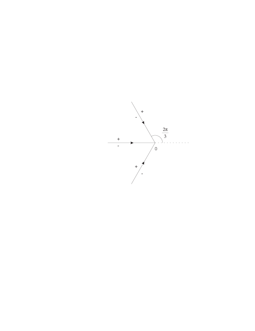
Figure 2: The contour $\Sigma_{\Psi}$

For our purpose here, it suffices to know the expression of $\Psi(\zeta)$ for $2\pi/3<\arg\zeta<\pi$. This is given in terms of the Hankel functions $H_{\alpha}^{(1)}$ and $H_{\alpha}^{(2)}$. For $2\pi/3<\arg\zeta<\pi$, we have

$$\Psi(\zeta)=\begin{pmatrix}\frac{1}{2}H_{\alpha}^{(1)}(2(-\zeta)^{1/2})&\frac{1}{2}H_{\alpha}^{(2)}(2(-\zeta)^{1/2})\\[4.30554pt] \pi\zeta^{1/2}\left(H_{\alpha}^{(1)}\right)^{\prime}(2(-\zeta)^{1/2})&\pi\zeta^{1/2}\left(H_{\alpha}^{(2)}\right)^{\prime}(2(-\zeta)^{1/2})\end{pmatrix}e^{\frac{1}{2}\alpha\pi i\sigma_{3}}.$$ (2.13)

The factor $E_{n}(z)$ in (2.10) is given by

$$E_{n}(z)=N(z)W(z)^{\sigma_{3}}\frac{1}{\sqrt{2}}\begin{pmatrix}1&-i\\ -i&1\end{pmatrix}f(z)^{\sigma_{3}/4}\left(2\pi n\right)^{\sigma_{3}/2}.$$ (2.14)

$E_{n}(z)$ is analytic in a full neighborhood of $U_{\delta}$.

There is a similar definition for the parametrix $\tilde{P}$ in a $\delta$ neighborhood $\tilde{U}_{\delta}$ of $-1$, see [12] for details.

We then have all the ingredients for the third transformation. We define

$$R(z) = S(z)N^{-1}(z),\qquad\mbox{for }z\in\mathbb{C}\setminus(\overline{U}_{\delta}\cup\overline{\tilde{U}}_{\delta}\cup\Sigma),$$ (2.15)

$$R(z) = S(z)P^{-1}(z),\qquad\mbox{for }z\in U_{\delta}\setminus\Sigma,$$ (2.16)

$$R(z) = S(z)\tilde{P}^{-1}(z),\qquad\mbox{for }z\in\tilde{U}_{\delta}\setminus\Sigma.$$ (2.17)

Then $R$ satisfies a RH problem with jumps on the system of contours $\Sigma_{R}$ shown in Figure 3.

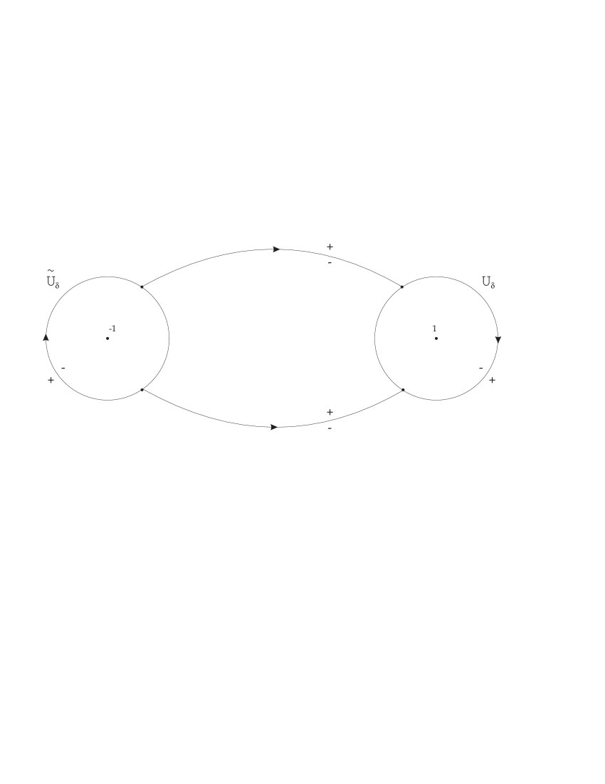
Figure 3: System of contours $\Sigma_{R}$

Note that $R$ depends on $n$, but the contour $\Sigma_{R}$ does not depend on $n$. The jump matrices for the RH problem for $R$ turn out to be uniformly close to the identity matrix with error term $O(\frac{1}{n})$. Then it follows that

$$R(z)=I+O\left(\frac{1}{n}\right),\qquad\mbox{as }n\to\infty,$$ (2.18)

uniformly for $z\in\mathbb{C}\setminus\Sigma_{R}$, and also, see [3, Section 8.1] in particular formulas (8.19) and (8.20),

$$\frac{d}{dz}R(z)=O\left(1\right),\qquad\mbox{as }n\to\infty,$$ (2.19)

uniformly for $z\in\mathbb{C}\setminus\Sigma_{R}$. In the following we will also use that

$$\det R(z)\equiv 1.$$ (2.20)

Remark 2.1

The asymptotic result (2.18) for $R$ may be refined and it is possible to obtain a full asymptotic expansion

$$R(z)\sim I+\sum_{k=1}^{\infty}\frac{R_{k}(z)}{n^{k}},\qquad\mbox{as }n\to\infty.$$

The matrix coefficients $R_{k}(z)$ are explicitly computable in function of $\alpha$, $\beta$, and the analytic factor $h$ in the modified Jacobi weight. The first two coefficients are computed in [12].

Remark 2.2

In [12] we also derived asymptotic expansions for the polynomials $p_{n}$ and $\pi_{n}$ uniformly valid in compact subsets of $\overline{\mathbb{C}}\setminus[-1,1]$, as well as asymptotic expansions for the leading coefficient $\gamma_{n}$ and for the coefficients in the recurrence relation satisfied by the orthonormal polynomials. For example, we have by [12, Theorem 1.4] uniformly for $z\in\mathbb{C}\setminus[-1,1]$,

$$\frac{2^{n}\pi_{n}(z)}{\varphi(z)}=\frac{D_{\infty}}{D(z)}\frac{\varphi(z)^{1/2}}{\sqrt{2}(z^{2}-1)^{1/4}}\left[1+O\left(\frac{1}{n}\right)\right],\qquad\mbox{as }n\to\infty.$$

The $O(\frac{1}{n})$ term can be developed into a complete asymptotic expansion in powers of $n^{-1}$.

The Riemann-Hilbert method also leads to strong asymptotics on the interval $(-1,1)$ and near the endpoints $\pm 1$. While these results are closely related to the asymptotics of $K_{n}$ as given in Theorem 1.1, we do not actually rely on them in the proof of Theorem 1.1. Therefore we state here the asymptotics of the orthogonal polynomials without proof. The proof is similar to the proof of Theorem 1.1, and in fact somewhat simpler. See also [4, 5].

As before, we let $\delta>0$ be the radius of the disks $U_{\delta}$ and $\tilde{U}_{\delta}$. Then we have for $x\in(-1+\delta,1-\delta)$,

$$\pi_{n}(x) = \frac{\sqrt{2}D_{\infty}}{2^{n}\sqrt{w(x)}(1-x^{2})^{1/4}}\left[R_{11}(x)\cos\left((n+1/2)\arccos x+\psi(x)-\frac{\pi}{4}\right)\right.$$ (2.21)

$$\qquad\qquad\left.-\frac{i}{D_{\infty}^{2}}R_{12}(x)\cos\left((n-1/2)\arccos x+\psi(x)-\frac{\pi}{4}\right)\right],$$

where $R_{11}(x)=1+O(\frac{1}{n})$ and $R_{12}(x)=O(\frac{1}{n})$ as $n\to\infty$, uniformly for $x\in(-1+\delta,1-\delta)$. The $O(\frac{1}{n})$ terms have a complete asymptotic expansion, see [12]. The function $\psi(x)$ in (2.21) is given by

$$\psi(x) = \frac{\sqrt{1-x^{2}}}{2\pi}\mathop{\hskip 1.16664pt\vbox{\hrule width=3.50002pt,height=0.5pt,depth=0.5pt}\hskip-4.66666pt}\mskip-3.0mu\intop\nolimits_{-1}^{1}\frac{\log w(t)}{\sqrt{1-t^{2}}}\frac{dt}{t-x}$$ (2.22)

$$= \frac{1}{2}\Bigl{(}\alpha(\arccos x-\pi)+\beta\arccos x\Bigr{)}+\frac{\sqrt{1-x^{2}}}{2\pi}\mathop{\hskip 1.16664pt\vbox{\hrule width=3.50002pt,height=0.5pt,depth=0.5pt}\hskip-4.66666pt}\mskip-3.0mu\intop\nolimits_{-1}^{1}\frac{\log h(t)}{\sqrt{1-t^{2}}}\frac{dt}{t-x},$$

where the integral is a Cauchy principal value integral. We remark that, under various assumptions, asymptotic results on the interval of orthogonality have been established by many authors, see for example [4, 5, 14, 15, 21, 25, 26].

For $x\in(1-\delta,1)$, the following is valid

$$\pi_{n}(x) = \frac{\sqrt{\pi}D_{\infty}}{2^{n}\sqrt{w(x)}}\frac{(n\arccos x)^{1/2}}{(1-x^{2})^{1/4}}\,\times$$ (2.23)

$$\left[R_{11}(x)\left(\cos\zeta_{1}(x)J_{\alpha}(n\arccos x)+\sin\zeta_{1}(x)J_{\alpha}^{\prime}(n\arccos x)\right)\right.$$

$$\qquad\left.-\frac{i}{D_{\infty}^{2}}R_{12}(x)\left(\cos\zeta_{2}(x)J_{\alpha}(n\arccos x)+\sin\zeta_{2}(x)J_{\alpha}^{\prime}(n\arccos x)\right)\right],$$

where $R_{11}(x)=1+O(\frac{1}{n})$ and $R_{12}(x)=O(\frac{1}{n})$ as $n\to\infty$, uniformly for $x\in(1-\delta,1)$, and where

$$\zeta_{1}(x)=\frac{1}{2}\arccos x+\psi(x)+\frac{\alpha\pi}{2},\qquad\zeta_{2}(x)=-\frac{1}{2}\arccos x+\psi(x)+\frac{\alpha\pi}{2},$$

with $\psi$ given by (2.22). There is an analogous expression for $x$ in the interval $(-1,-1+\delta)$.

3 Proof of Theorem 1.1 and Corollary 1.2

In this section we prove Theorem 1.1 and Corollary 1.2. We follow the work of Deift et al. [3, 4]. Recall that

$$K_{n}(x,y) = \sqrt{w(x)}\sqrt{w(y)}\,\frac{\gamma_{n-1}}{\gamma_{n}}\,\frac{p_{n}(x)p_{n-1}(y)-p_{n-1}(x)p_{n}(y)}{x-y}$$

$$= \sqrt{w(x)}\sqrt{w(y)}\,\gamma_{n-1}^{2}\,\frac{\pi_{n}(x)\pi_{n-1}(y)-\pi_{n-1}(x)\pi_{n}(y)}{x-y},$$

where $\pi_{n}$ is the monic orthogonal polynomial of degree $n$ with respect to the modified Jacobi weight $w$. As in [3, 4] we replace the polynomials $\pi_{n-1}$ and $\pi_{n}$ by the appropriate entries of $Y$, see (2.5), to obtain

$$K_{n}(x,y)=-\frac{1}{2\pi i}\sqrt{w(x)}\sqrt{w(y)}\,\frac{Y_{11}(x)Y_{21}(y)-Y_{21}(x)Y_{11}(y)}{x-y}.$$ (3.1)

Thus, $K_{n}$ can be expressed in terms of the first column of $Y$. The asymptotic behavior of $Y$ follows from the transformations $Y\mapsto T\mapsto S\mapsto R$ described in section 2, and the behavior (2.18)–(2.20) of $R$.

3.1 Proof of Theorem 1.1 (a)

We will first express $Y_{11}$ and $Y_{21}$ in terms of $R$. In the following, $\delta>0$ will be a small but fixed number. This number is the radius of the disks $U_{\delta}$ and $\tilde{U}_{\delta}$ used in the local RH analysis around $\pm 1$.

Lemma 3.1

We have for $x\in(-1+\delta,1-\delta)$,

$$\begin{pmatrix}Y_{11}(x)\\ Y_{21}(x)\end{pmatrix}=\frac{1}{\sqrt{w(x)}}\,2^{-n\sigma_{3}}L_{+}(x)\begin{pmatrix}e^{in\arccos x}\\ e^{-in\arccos x}\end{pmatrix},$$ (3.2)

with $L(z)$ given by

$$L(z)=R(z)D_{\infty}^{\sigma_{3}}\begin{pmatrix}\frac{a(z)+a(z)^{-1}}{2}&\frac{a(z)-a(z)^{-1}}{2i}\\[4.30554pt] \frac{a(z)-a(z)^{-1}}{-2i}&\frac{a(z)+a(z)^{-1}}{2}\end{pmatrix}e^{i\psi(z)\sigma_{3}},$$ (3.3)

where

$$\psi(x)=\frac{1}{2}\Bigl{(}\alpha(\arccos x-\pi)+\beta\arccos x\Bigr{)}+\frac{\sqrt{1-x^{2}}}{2\pi}\mathop{\hskip 1.16664pt\vbox{\hrule width=3.50002pt,height=0.5pt,depth=0.5pt}\hskip-4.66666pt}\mskip-3.0mu\intop\nolimits_{-1}^{1}\frac{\log h(t)}{\sqrt{1-t^{2}}}\frac{dt}{t-x}.$$ (3.4)

The matrices $L_{+}(x)$ and $\frac{d}{dx}L_{+}(x)$ are uniformly bounded for $x\in(-1+\delta,1-\delta)$ as $n\to\infty$, and

$$\det L_{+}(x)\equiv 1,\qquad\mbox{for }x\in(-1+\delta,1-\delta).$$ (3.5)

Remark 3.2

The singular integral (3.4) is being understood in the sense of the principal value. It may be shown that $D_{+}(x)=\sqrt{w(x)}\exp(-i\psi(x))$ so that $-\psi(x)$ is the argument of the Szegő function on the interval.

• We use the series of transformations $Y\mapsto T\mapsto S\mapsto R$ and we unfold them for $z$ in the upper part of the lens but outside the disks $U_{\delta}$ and $\tilde{U}_{\delta}$, and then take the limit to the interval $(-1+\delta,1-\delta)$. Thus, let $z$ be in the upper part of the lens but outside the disks $U_{\delta}$ and $\tilde{U}_{\delta}$. We then have by (2.6), (2.7) and (2.15)

  $$Y(z)=2^{-n\sigma_{3}}R(z)N(z)\begin{pmatrix}\varphi(z)^{n}&0\\ w(z)^{-1}\varphi(z)^{-n}&\varphi(z)^{-n}\end{pmatrix}.$$ (3.6)

  Inserting the expression (2.9) for $N$ into (3.6), we obtain for the first column of $Y$

  $$\begin{pmatrix}Y_{11}(z)\\ Y_{21}(z)\end{pmatrix}=2^{-n\sigma_{3}}R(z)D_{\infty}^{\sigma_{3}}\begin{pmatrix}\frac{a(z)+a(z)^{-1}}{2}&\frac{a(z)-a(z)^{-1}}{2i}\\[4.30554pt] \frac{a(z)-a(z)^{-1}}{-2i}&\frac{a(z)+a(z)^{-1}}{2}\end{pmatrix}\begin{pmatrix}\frac{1}{D(z)}\,\varphi(z)^{n}\\[8.61108pt] \frac{D(z)}{w(z)}\,\varphi(z)^{-n}\end{pmatrix}.$$ (3.7)

  We now take the limit $z\to x\in(-1+\delta,1-\delta)$. Since $D_{+}(x)=\sqrt{w(x)}e^{-i\psi(x)}$ and $\varphi_{+}(x)=\exp(i\arccos x)$, (3.2) now follows from (3.7).

  Note that $R(x)$ and $\frac{d}{dx}R(x)$ are uniformly bounded for $x\in(-1+\delta,1-\delta)$ as $n\to\infty$. Let $U$ be a neighborhood of $[-1,1]$ such that $\log h$ is defined and analytic in $U$, and let $\gamma$ be a closed contour in $U\setminus[-1,1]$ encircling the interval $[-1,1]$ once in the positive direction. Via contour deformation, we may write $\psi$ in the form

  $$\psi(x)=\frac{1}{2}\Bigl{(}\alpha(\arccos x-\pi)+\beta\arccos x\Bigr{)}+\frac{\sqrt{1-x^{2}}}{4\pi i}\oint_{\gamma}\frac{\log h(\zeta)}{(\zeta^{2}-1)^{1/2}}\frac{d\zeta}{\zeta-x}.$$

  Thus $\psi$ has an analytic extension to a neighborhood of $(-1,1)$. This implies that $\psi$ and its derivative are bounded on $(-1+\delta,1-\delta)$. From the explicit form (3.3) of $L_{+}$ we then find that $L_{+}(x)$ and $\frac{d}{dx}L_{+}(x)$ are uniformly bounded for $x\in(-1+\delta,1-\delta)$ as $n\to\infty$. Since $\det R(z)\equiv 1$ it is easy to see from (3.3) that $\det L_{+}(x)\equiv 1$. $\Box$

• of Theorem 1.1 (a) Letting $y\to x$ in (3.1) we get

  $$K_{n}(x,x) = \frac{1}{2\pi i}w(x)\left(Y_{11}(x)Y^{\prime}_{21}(x)-Y_{21}(x)Y^{\prime}_{11}(x)\right)$$ (3.8)

  $$= \frac{1}{2\pi i}\det\begin{pmatrix}\sqrt{w(x)}Y_{11}(x)&\sqrt{w(x)}Y^{\prime}_{11}(x)\\ \sqrt{w(x)}Y_{21}(x)&\sqrt{w(x)}Y^{\prime}_{21}(x)\end{pmatrix}$$

  $$= \frac{1}{2\pi i}\det\begin{pmatrix}2^{n}\sqrt{w(x)}Y_{11}(x)&\frac{d}{dx}\left(2^{n}\sqrt{w(x)}Y_{11}(x)\right)\\ 2^{-n}\sqrt{w(x)}Y_{21}(x)&\frac{d}{dx}\left(2^{-n}\sqrt{w(x)}Y_{21}(x)\right)\end{pmatrix}.$$

  By (3.2) the matrix in (3.8) is equal to

  $$L_{+}(x)\begin{pmatrix}e^{in\arccos x}&-\frac{in}{\sqrt{1-x^{2}}}e^{in\arccos x}\\ e^{-in\arccos x}&\frac{in}{\sqrt{1-x^{2}}}e^{-in\arccos x}\end{pmatrix}+\left(\frac{d}{dx}L_{+}(x)\right)\begin{pmatrix}0&e^{in\arccos x}\\ 0&e^{-in\arccos x}\end{pmatrix}$$

  $$=L_{+}(x)e^{in\arccos x\sigma_{3}}\begin{pmatrix}1&-\frac{in}{\sqrt{1-x^{2}}}\\ 1&\frac{in}{\sqrt{1-x^{2}}}\end{pmatrix}+\left(\frac{d}{dx}L_{+}(x)\right)\begin{pmatrix}0&e^{in\arccos x}\\ 0&e^{-in\arccos x}\end{pmatrix}.$$

  Since $L_{+}(x)$ and $e^{in\arccos x\sigma_{3}}$ have determinant one, it follows that

  $$K_{n}(x,x)=\frac{1}{2\pi i}\det\left[\begin{pmatrix}1&-\frac{in}{\sqrt{1-x^{2}}}\\ 1&\frac{in}{\sqrt{1-x^{2}}}\end{pmatrix}+e^{-in\arccos x\sigma_{3}}L_{+}^{-1}(x)\left(\frac{d}{dx}L_{+}(x)\right)\begin{pmatrix}0&e^{in\arccos x}\\ 0&e^{-in\arccos x}\end{pmatrix}\right].$$ (3.9)

  The entries of $L_{+}(x)$ and $\frac{d}{dx}L_{+}(x)$ are uniformly bounded by Lemma 3.1. Since $\det L_{+}(x)=1$, also the entries of $L_{+}^{-1}(x)$ are uniformly bounded. Thus, we have uniformly for $x\in(-1+\delta,1-\delta)$,

  $$K_{n}(x,x) = \frac{1}{2\pi i}\det\begin{pmatrix}1&-\frac{in}{\sqrt{1-x^{2}}}+O(1)\\ 1&\frac{in}{\sqrt{1-x^{2}}}+O(1)\end{pmatrix}=\frac{1}{2\pi i}\left(\frac{2in}{\sqrt{1-x^{2}}}+O(1)\right)$$

  $$= \frac{n}{\pi\sqrt{1-x^{2}}}+O(1).$$

  This proves part (a) of Theorem 1.1. $\Box$

3.2 Proof of Theorem 1.1 (b)

• of Theorem 1.1 (b) Let $x\in(-1,1)$ and $u,v\in\mathbb{R}$. For the sake of brevity, we use $u_{x,n}$ and $v_{x,n}$ to denote $x+\frac{u}{n\xi(x)}$ and $x+\frac{v}{n\xi(x)}$, respectively. We write

  $$\widehat{K}_{n}(u,v)=\frac{1}{n\xi(x)}K_{n}(u_{x,n},v_{x,n}).$$

  From (3.1) we then have

  $$\widehat{K}_{n}(u,v) = -\frac{1}{2\pi i(u-v)}\sqrt{w(u_{x,n})}\sqrt{w(v_{x,n})}\det\begin{pmatrix}Y_{11}(u_{x,n})&Y_{11}(v_{x,n})\\ Y_{21}(u_{x,n})&Y_{21}(v_{x,n})\end{pmatrix}$$ (3.10)

  $$= -\frac{1}{2\pi i(u-v)}\det\begin{pmatrix}2^{n}\sqrt{w(u_{x,n})}Y_{11}(u_{x,n})&2^{n}\sqrt{w(v_{x,n})}Y_{11}(v_{x,n})\\ 2^{-n}\sqrt{w(u_{x,n})}Y_{21}(u_{x,n})&2^{-n}\sqrt{w(v_{x,n})}Y_{21}(v_{x,n})\end{pmatrix}.$$

  Next, we use the expression (3.2) for $Y_{11}$ and $Y_{21}$ in (3.10) to obtain

  $$\widehat{K}_{n}(u,v) = -\frac{1}{2\pi i(u-v)}\det\left[L_{+}(u_{x,n})\begin{pmatrix}e^{in\arccos u_{x,n}}&0\\ e^{-in\arccos u_{x,n}}&0\end{pmatrix}\right.$$ (3.11)

  $$+\,\left.L_{+}(v_{x,n})\begin{pmatrix}0&e^{in\arccos v_{x,n}}\\ 0&e^{-in\arccos v_{x,n}}\end{pmatrix}\right]$$

  $$= -\frac{1}{2\pi i(u-v)}\det\left[L_{+}(v_{x,n})\begin{pmatrix}e^{in\arccos u_{x,n}}&e^{in\arccos v_{x,n}}\\ e^{-in\arccos u_{x,n}}&e^{-in\arccos v_{x,n}}\end{pmatrix}\right.$$

  $$\left.+\,\left[L_{+}(u_{x,n})-L_{+}(v_{x,n})\right]\begin{pmatrix}e^{in\arccos u_{x,n}}&0\\ e^{-in\arccos u_{x,n}}&0\end{pmatrix}\right].$$

  Since $\det L_{+}(v_{x,n})=1$, we then get

  $$\widehat{K}_{n}(u,v) = -\frac{1}{2\pi i(u-v)}\det\left[\begin{pmatrix}e^{in\arccos u_{x,n}}&e^{in\arccos v_{x,n}}\\ e^{-in\arccos u_{x,n}}&e^{-in\arccos v_{x,n}}\end{pmatrix}\right.$$ (3.12)

  $$\left.+\,L_{+}^{-1}(v_{x,n})\left[L_{+}(u_{x,n})-L_{+}(v_{x,n})\right]\begin{pmatrix}e^{in\arccos u_{x,n}}&0\\ e^{-in\arccos u_{x,n}}&0\end{pmatrix}\right].$$

  Since $\frac{d}{dx}L_{+}(x)$ is uniformly bounded as $n\to\infty$, we have by the mean value theorem

  $$L_{+}(u_{x,n})-L_{+}(v_{x,n})=O\left(u_{x,n}-v_{x,n}\right)=O\left(\frac{u-v}{n}\right),$$

  uniformly for $x\in(-1+\delta,1-\delta)$ and for $u,v$ in compact subsets of $\mathbb{R}$. Since $L_{+}(x)$ is uniformly bounded, and $\det L_{+}(x)=1$, we have that $L_{+}^{-1}(v_{x,n})$ is uniformly bounded as well, so that

  $$L_{+}^{-1}(v_{x,n})[L_{+}(u_{x,n})-L_{+}(v_{x,n})]\begin{pmatrix}e^{in\arccos u_{x,n}}&0\\ e^{-in\arccos u_{x,n}}&0\end{pmatrix}=\begin{pmatrix}O\left(\frac{u-v}{n}\right)&0\\[4.30554pt] O\left(\frac{u-v}{n}\right)&0\end{pmatrix}.$$ (3.13)

  Thus by (3.12) and (3.13)

  $$\widehat{K}_{n}(u,v) = -\frac{1}{2\pi i(u-v)}\det\begin{pmatrix}e^{in\arccos u_{x,n}}+O\left(\frac{u-v}{n}\right)&e^{in\arccos v_{x,n}}\\[4.30554pt] e^{-in\arccos u_{x,n}}+O\left(\frac{u-v}{n}\right)&e^{-in\arccos v_{x,n}}\end{pmatrix}$$ (3.14)

  $$= -\frac{1}{2\pi i(u-v)}\det\begin{pmatrix}e^{in\arccos u_{x,n}}&e^{in\arccos v_{x,n}}\\ e^{-in\arccos u_{x,n}}&e^{-in\arccos v_{x,n}}\end{pmatrix}+O\left(\frac{1}{n}\right)$$

  $$= -\frac{1}{2\pi i(u-v)}\left(e^{in(\arccos u_{x,n}-\arccos v_{x,n})}-e^{-in(\arccos u_{x,n}-\arccos v_{x,n})}\right)+O\left(\frac{1}{n}\right)$$

  $$= -\frac{\sin(n(\arccos u_{x,n}-\arccos v_{x,n}))}{\pi(u-v)}+O\left(\frac{1}{n}\right),$$

  uniformly for $x\in(-1+\delta,1-\delta)$ and $u,v$ in compact subsets of $\mathbb{R}$. Since

  $$n(\arccos u_{x,n}-\arccos v_{x,n})=-\pi(u-v)(1+O(1/n)),\qquad\mbox{as $n\to\infty$,}$$

  also uniformly for $x\in(-1+\delta,1-\delta)$ and $u,v$ in compact subsets of $\mathbb{R}$, part (b) of Theorem 1.1 follows. $\Box$

3.3 Proof of Theorem 1.1 (c)

To prove part (c) of Theorem 1.1, we start with a result similar to Lemma 3.1.

Lemma 3.3

For $x\in(1-\delta,1)$, we have

$$\begin{pmatrix}Y_{11}(x)\\ Y_{21}(x)\end{pmatrix}=\sqrt{\frac{2\pi n}{w(x)}}\,2^{-n\sigma_{3}}M_{+}(x)\begin{pmatrix}J_{\alpha}(n\arccos x)\\ \frac{i}{2}\arccos xJ^{\prime}_{\alpha}(n\arccos x)\end{pmatrix},$$ (3.15)

with $M(z)$ given by

$$M(z)=R(z)N(z)W(z)^{\sigma_{3}}\frac{1}{\sqrt{2}}\begin{pmatrix}1&-i\\ -i&1\end{pmatrix}f(z)^{\sigma_{3}/4},$$ (3.16)

where $R$ is the result of the transformations $Y\mapsto T\mapsto S\mapsto R$ of the RH problem, the matrix valued function $N$ is given by (2.9), and the scalar functions $f$ and $W$ are given by (2.11) and (2.12), respectively.

$M$ is analytic in $U_{\delta}$ with $M(z)$ and $\frac{d}{dz}M(z)$ uniformly bounded for $z\in U_{\delta}$ as $n\to\infty$. Furthermore, we have

$$\det M(z)\equiv 1.$$

• As in the proof of Lemma 3.1 we unravel the transformations $Y\mapsto T\mapsto S\mapsto R$, but now for $z$ in the upper part of the lens and inside the disk $U_{\delta}$. We then have by (2.6), (2.7), (2.10) and (2.16)

  $$Y(z)=2^{-n\sigma_{3}}R(z)E_{n}(z)\Psi\left(n^{2}f(z)\right)W(z)^{-\sigma_{3}}\begin{pmatrix}1&0\\ w(z)^{-1}&1\end{pmatrix}.$$ (3.17)

  Since ${\rm Im\,}z>0$, we have by (2.12) that $W(z)=w^{1/2}(z)e^{i\pi\alpha/2}$. Inserting this into (3.17) we get for the first column of $Y$

  $$\begin{pmatrix}Y_{11}(z)\\ Y_{21}(z)\end{pmatrix}=w^{-1/2}(z)2^{-n\sigma_{3}}R(z)E_{n}(z)\Psi\left(n^{2}f(z)\right)\begin{pmatrix}e^{-i\pi\alpha/2}\\ e^{i\pi\alpha/2}\end{pmatrix}.$$ (3.18)

  Since $z$ is in the upper part of the lens and inside the disk $U_{\delta}$, we have $2\pi/3<\arg n^{2}f(z)<\pi$, see [12, section 6], and we thus use (2.13) to evaluate $\Psi(n^{2}f(z))$. From formulas 9.1.3 and 9.1.4 of [1] we then have

  $$\Psi\left(n^{2}f(z)\right)\begin{pmatrix}e^{-i\pi\alpha/2}\\ e^{i\pi\alpha/2}\end{pmatrix}=\begin{pmatrix}J_{\alpha}(2n(-f(z))^{1/2})\\[4.30554pt] 2\pi nf^{1/2}(z)J^{\prime}_{\alpha}(2n(-f(z))^{1/2})\end{pmatrix}.$$ (3.19)

  By (2.14) and (3.16) we have $R(z)E_{n}(z)=M(z)(2\pi n)^{\sigma_{3}/2}$. Inserting this and (3.19) into (3.18) we get

  $$\begin{pmatrix}Y_{11}(z)\\ Y_{21}(z)\end{pmatrix}=\frac{\sqrt{2\pi n}}{w^{1/2}(z)}2^{-n\sigma_{3}}M(z)\begin{pmatrix}J_{\alpha}(2n(-f(z))^{1/2})\\[4.30554pt] f^{1/2}(z)J^{\prime}_{\alpha}(2n(-f(z))^{1/2})\end{pmatrix}.$$ (3.20)

  We now take the limit $z\to x\in(1-\delta,1)$. By (2.11), and since $\varphi_{+}(x)=\exp(i\arccos x)$ we have $f^{1/2}_{+}(x)=\frac{i}{2}\arccos x$, so that $2(-f_{+}(x))^{1/2}=\arccos x$. Inserting this into (3.20), we obtain (3.15).

$M$ is analytic in $U_{\delta}$ since both $E_{n}$, see [12, Proposition 6.5], and $R$ are analytic in $U_{\delta}$. So, we may write $M(x)$ instead of $M_{+}(x)$ in (3.15).

By (2.18) and (2.19) we have that $R(z)$ and $\frac{d}{dz}R(z)$ are uniformly bounded for $z\in U_{\delta}$ as $n\to\infty$. Since

$$N(z)W(z)^{\sigma_{3}}\frac{1}{\sqrt{2}}\begin{pmatrix}1&-i\\ -i&1\end{pmatrix}f(z)^{\sigma_{3}/4}$$

is analytic for $z\in U_{\delta}$ and does not depend on $n$, we have from (3.16) that also $M(z)$ and $\frac{d}{dz}M(z)$ are uniformly bounded for $z\in U_{\delta}$ as $n\to\infty$.

The fact that $\det M(z)\equiv 1$ follows easily from (2.9), (2.20), and (3.16). $\Box$

Remark 3.4

We check that (3.15) yields $\begin{pmatrix}Y_{11}(x)\\ Y_{21}(x)\end{pmatrix}=O(1)$ as $x\nearrow 1$, which is in agreement with the fact that $Y_{11}$ and $Y_{21}$ are polynomials, see (2.5). Since $\arccos x=O\left((1-x)^{1/2}\right)$ as $x\nearrow 1$, we have by formula 9.1.10 of [1]

$$\begin{pmatrix}J_{\alpha}(n\arccos x)\\ \arccos x\,J^{\prime}_{\alpha}(n\arccos x)\end{pmatrix}=\begin{pmatrix}O\left((1-x)^{\alpha/2}\right)\\ O\left((1-x)^{\alpha/2}\right)\end{pmatrix},\qquad\mbox{as }x\nearrow 1.$$ (3.21)

Since $M$ is analytic near 1, see Lemma 3.3, we have $M(x)=O(1)$ as $x\nearrow 1$. Inserting (3.21) into (3.15) and noting that $w(x)^{-1}=O((1-x)^{-\alpha})$ as $x\nearrow 1$, we then have indeed that $Y_{11}(x)$ and $Y_{21}(x)$ remain bounded as $x\nearrow 1$.

We also need the asymptotic behavior of $J_{\alpha}(\tilde{u}_{n})$ and $J^{\prime}_{\alpha}(\tilde{u}_{n})$ as $n\to\infty$, where we put $u_{n}=1-\frac{u}{2n^{2}}$ and $\tilde{u}_{n}=n\arccos u_{n}$. These will be contained in the next lemma.

Lemma 3.5

Let $u\in(0,\infty)$, $u_{n}=1-\frac{u}{2n^{2}}$, and $\tilde{u}_{n}=n\arccos u_{n}$. We then have as $n\to\infty$,

$$\tilde{u}_{n}=\sqrt{u}+O\left(\frac{u^{\frac{3}{2}}}{n^{2}}\right),$$ (3.22)

$$J_{\alpha}(\tilde{u}_{n})=J_{\alpha}(\sqrt{u})+O\left(\frac{u^{\frac{\alpha}{2}+1}}{n^{2}}\right),$$ (3.23)

$$J^{\prime}_{\alpha}(\tilde{u}_{n})=J^{\prime}_{\alpha}(\sqrt{u})+O\left(\frac{u^{\frac{\alpha}{2}+\frac{1}{2}}}{n^{2}}\right).$$ (3.24)

The error terms hold uniformly for $u$ in bounded subsets of $(0,\infty)$.

• Since $z^{-1/2}\arccos(1-z)$ is analytic in a neighborhood of $0$ with expansion

  $$z^{-1/2}\arccos(1-z)=\sqrt{2}+O(z),\qquad\mbox{as $z\to 0$,}$$

  we easily get (3.22).

  By formula 9.1.10 of [1] we know that $J_{\alpha}(z)=z^{\alpha}G(z)$ with $G$ an entire function. From (3.22) and Taylor’s formula we then get uniformly for $u$ in bounded subsets of $(0,\infty)$,

  $$J_{\alpha}(n\arccos u_{n}) = u^{\frac{\alpha}{2}}\left(1+O\left(\frac{u}{n^{2}}\right)\right)\left(G(\sqrt{u})+O\left(\frac{u^{\frac{3}{2}}}{n^{2}}\right)\right)$$

  $$= J_{\alpha}(\sqrt{u})+O\left(\frac{u^{\frac{\alpha}{2}+1}}{n^{2}}\right),$$

  which is (3.23). The proof of (3.24) follows in a similar fashion, using

  $$J^{\prime}_{\alpha}(z)=\alpha z^{\alpha-1}G(z)+z^{\alpha}G^{\prime}(z),$$

  and Taylor’s formula again. $\Box$

Now we are ready for the proof of our main result.

• of Theorem 1.1 (c) Let $u,v\in(0,\infty)$ and define

  $$u_{n}=1-\frac{u}{2n^{2}},\quad v_{n}=1-\frac{v}{2n^{2}},\qquad\tilde{u}_{n}=n\arccos u_{n},\quad\tilde{v}_{n}=n\arccos v_{n}.$$ (3.25)

  We put

  $$D_{n}(u,v)=\frac{1}{2n^{2}}K_{n}(u_{n},v_{n}).$$ (3.26)

  From (3.1) we then have

  $$D_{n}(u,v) = \frac{1}{2\pi i(u-v)}\sqrt{w(u_{n})}\sqrt{w(v_{n})}\det\begin{pmatrix}Y_{11}(u_{n})&Y_{11}(v_{n})\\ Y_{21}(u_{n})&Y_{21}(v_{n})\end{pmatrix}$$ (3.27)

  $$= \frac{1}{2\pi i(u-v)}\det\begin{pmatrix}2^{n}\sqrt{w(u_{n})}Y_{11}(u_{n})&2^{n}\sqrt{w(v_{n})}Y_{11}(v_{n})\\ 2^{-n}\sqrt{w(u_{n})}Y_{21}(u_{n})&2^{-n}\sqrt{w(v_{n})}Y_{21}(v_{n})\end{pmatrix}.$$

  Next, we replace the two columns in the determinant in (3.27) by the expression (3.15) we found in Lemma 3.3. It follows that

  $$D_{n}(u,v)=\frac{2\pi n}{2\pi i(u-v)}\det\left[M(u_{n})\begin{pmatrix}J_{\alpha}(\tilde{u}_{n})&0\\[4.30554pt] \frac{i}{2n}\tilde{u}_{n}J^{\prime}_{\alpha}(\tilde{u}_{n})&0\end{pmatrix}+M(v_{n})\begin{pmatrix}0&J_{\alpha}(\tilde{v}_{n})\\[4.30554pt] 0&\frac{i}{2n}\tilde{v}_{n}J^{\prime}_{\alpha}(\tilde{v}_{n})\end{pmatrix}\right].\qquad$$ (3.28)

  We rewrite the matrix appearing in the determinant in (3.28) as

  $$M(v_{n})\left[\begin{pmatrix}J_{\alpha}(\tilde{u}_{n})&J_{\alpha}(\tilde{v}_{n})\\[4.30554pt] \frac{i}{2n}\tilde{u}_{n}J^{\prime}_{\alpha}(\tilde{u}_{n})&\frac{i}{2n}\tilde{v}_{n}J^{\prime}_{\alpha}(\tilde{v}_{n})\end{pmatrix}+M(v_{n})^{-1}\bigl{[}M(u_{n})-M(v_{n})\bigr{]}\begin{pmatrix}J_{\alpha}(\tilde{u}_{n})&0\\[4.30554pt] \frac{i}{2n}\tilde{u}_{n}J^{\prime}_{\alpha}(\tilde{u}_{n})&0\end{pmatrix}\right].$$

  Now we use $\det M(v_{n})=1$ and the fact that $M(z)$ is uniformly bounded for $z\in U_{\delta}$, see Lemma 3.3, to conclude that the entries of $M(v_{n})^{-1}$ are uniformly bounded. By Lemma 3.3, we also have that $\frac{d}{dz}M(z)$ is uniformly bounded so that $M(u_{n})-M(v_{n})=O\left(\frac{u-v}{n^{2}}\right)$. From Lemma 3.5 it follows that $J_{\alpha}(\tilde{u}_{n})=O(u^{\alpha/2})$ and $\tilde{u}_{n}J^{\prime}_{\alpha}(\tilde{u}_{n})=O(u^{\alpha/2})$ uniformly for $u$ in bounded subsets of $(0,\infty)$ as $n\to\infty$. Hence we have, uniformly for $u,v$ in bounded subsets of $(0,\infty)$,

  $$M(v_{n})^{-1}\bigl{[}M(u_{n})-M(v_{n})\bigr{]}\begin{pmatrix}J_{\alpha}(\tilde{u}_{n})&0\\[4.30554pt] \frac{i}{2n}\tilde{u}_{n}J^{\prime}_{\alpha}(\tilde{u}_{n})&0\end{pmatrix}=\begin{pmatrix}O\left(\frac{u-v}{n^{2}}\,u^{\frac{\alpha}{2}}\right)&0\\[4.30554pt] O\left(\frac{u-v}{n^{2}}\,u^{\frac{\alpha}{2}}\right)&0\end{pmatrix}.$$ (3.29)

  It now follows that (we use $\det M(v_{n})=1$)

  $$D_{n}(u,v)=\frac{1}{2(u-v)}\det\begin{pmatrix}J_{\alpha}(\tilde{u}_{n})+O\left(\frac{u-v}{n^{2}}\,u^{\frac{\alpha}{2}}\right)&J_{\alpha}(\tilde{v}_{n})\\[4.30554pt] \tilde{u}_{n}J^{\prime}_{\alpha}(\tilde{u}_{n})+O\left(\frac{u-v}{n}\,u^{\frac{\alpha}{2}}\right)&\tilde{v}_{n}J^{\prime}_{\alpha}(\tilde{v}_{n})\end{pmatrix}.$$ (3.30)

  Since $J_{\alpha}(\tilde{v}_{n})=O(v^{\alpha/2})$ and $\tilde{v}_{n}J^{\prime}_{\alpha}(\tilde{v}_{n})=O(v^{\alpha/2})$ as $n\to\infty$, we then get uniformly for $u,v$ in bounded subsets of $(0,\infty)$,

  $$D_{n}(u,v)=\frac{1}{2(u-v)}\det\begin{pmatrix}J_{\alpha}(\tilde{u}_{n})&J_{\alpha}(\tilde{v}_{n})\\[4.30554pt] \tilde{u}_{n}J^{\prime}_{\alpha}(\tilde{u}_{n})&\tilde{v}_{n}J^{\prime}_{\alpha}(\tilde{v}_{n})\end{pmatrix}+O\left(\frac{u^{\frac{\alpha}{2}}v^{\frac{\alpha}{2}}}{n}\right).$$ (3.31)

  In the determinant in (3.31) we can replace $\tilde{u}_{n}$ and $\tilde{v}_{n}$ by $\sqrt{u}$ and $\sqrt{v}$ respectively, and make an error which we could estimate using Lemma 3.5. However, this estimate would not be uniform for $u-v$ close to zero. So we will be more careful. We bring in a factor $u^{-\frac{\alpha}{2}}$ into the first column of the determinant in (3.31) and a factor $v^{-\frac{\alpha}{2}}$ into the second. Then we subtract the second column from the first to obtain

  $$D_{n}(u,v)=\frac{u^{\frac{\alpha}{2}}v^{\frac{\alpha}{2}}}{2(u-v)}\det\begin{pmatrix}u^{-\frac{\alpha}{2}}J_{\alpha}(\tilde{u}_{n})-v^{-\frac{\alpha}{2}}J_{\alpha}(\tilde{v}_{n})&v^{-\frac{\alpha}{2}}J_{\alpha}(\tilde{v}_{n})\\[4.30554pt] u^{-\frac{\alpha}{2}}\tilde{u}_{n}J^{\prime}_{\alpha}(\tilde{u}_{n})-v^{-\frac{\alpha}{2}}\tilde{v}_{n}J^{\prime}_{\alpha}(\tilde{v}_{n})&v^{-\frac{\alpha}{2}}\tilde{v}_{n}J^{\prime}_{\alpha}(\tilde{v}_{n})\end{pmatrix}+O\left(\frac{u^{\frac{\alpha}{2}}v^{\frac{\alpha}{2}}}{n}\right).\ \$$ (3.32)

  From Lemma 3.5 it follows that uniformly for $x$ in bounded subsets of $(0,\infty)$,

  $$\frac{d}{dx}\left(x^{-\frac{\alpha}{2}}J_{\alpha}(n\arccos x_{n})-x^{-\frac{\alpha}{2}}J_{\alpha}(\sqrt{x})\right)=O\left(\frac{1}{n^{2}}\right).$$

  Then it easily follows that the $1,1$-entry in the determinant in (3.32) is equal to

  $$u^{-\frac{\alpha}{2}}J_{\alpha}(\sqrt{u})-v^{-\frac{\alpha}{2}}J_{\alpha}(\sqrt{v})+O\left(\frac{u-v}{n^{2}}\right).$$

  Similarly, if we use

  $$\frac{d}{dx}\left(x^{-\frac{\alpha}{2}}n\arccos x_{n}J^{\prime}_{\alpha}(n\arccos x_{n})-x^{-\frac{\alpha}{2}}\sqrt{x}J^{\prime}_{\alpha}(\sqrt{x})\right)=O\left(\frac{1}{n^{2}}\right),$$

  we find that the $2,1$-entry is

  $$u^{-\frac{\alpha}{2}}\sqrt{u}J^{\prime}_{\alpha}(\sqrt{u})-v^{-\frac{\alpha}{2}}\sqrt{v}J^{\prime}_{\alpha}(\sqrt{v})+O\left(\frac{u-v}{n^{2}}\right).$$

  From Lemma 3.5 it also follows that we may replace $\tilde{v}_{n}$ by $\sqrt{v}$ in the second column at the expense of an error term $O(\frac{1}{n^{2}})$. Therefore, uniformly for $u,v$ in bounded subsets of $(0,\infty)$,

  $$D_{n}(u,v)=\frac{u^{\frac{\alpha}{2}}v^{\frac{\alpha}{2}}}{2(u-v)}$$ (3.33)

  $$\,\times\,\det\begin{pmatrix}u^{-\frac{\alpha}{2}}J_{\alpha}(\sqrt{u})-v^{-\frac{\alpha}{2}}J_{\alpha}(\sqrt{v})+O\left(\frac{u-v}{n^{2}}\right)&v^{-\frac{\alpha}{2}}J_{\alpha}(\sqrt{v})+O\left(\frac{1}{n^{2}}\right)\\[4.30554pt] u^{-\frac{\alpha}{2}}\sqrt{u}J^{\prime}_{\alpha}(\sqrt{u})-v^{-\frac{\alpha}{2}}\sqrt{v}J^{\prime}_{\alpha}(\sqrt{v})+O\left(\frac{u-v}{n^{2}}\right)&v^{-\frac{\alpha}{2}}\sqrt{v}J^{\prime}_{\alpha}(\sqrt{v})+O\left(\frac{1}{n^{2}}\right)\end{pmatrix}$$

  $$\qquad+\,O\left(\frac{u^{\frac{\alpha}{2}}v^{\frac{\alpha}{2}}}{n}\right)$$

  $$=\mathbb{J}_{\alpha}(u,v)+\frac{u^{\frac{\alpha}{2}}v^{\frac{\alpha}{2}}}{2(u-v)}\det\begin{pmatrix}u^{-\frac{\alpha}{2}}J_{\alpha}(\sqrt{u})-v^{-\frac{\alpha}{2}}J_{\alpha}(\sqrt{v})&O\left(\frac{1}{n^{2}}\right)\\[4.30554pt] u^{-\frac{\alpha}{2}}\sqrt{u}J^{\prime}_{\alpha}(\sqrt{u})-v^{-\frac{\alpha}{2}}\sqrt{v}J^{\prime}_{\alpha}(\sqrt{v})&O\left(\frac{1}{n^{2}}\right)\end{pmatrix}$$

  $$\qquad+\,O\left(\frac{u^{\frac{\alpha}{2}}v^{\frac{\alpha}{2}}}{n}\right).$$

  Since $z^{-\alpha/2}J_{\alpha}(\sqrt{z})$ is an entire function we get by the mean value theorem that

  $$\frac{u^{-\frac{\alpha}{2}}J_{\alpha}(\sqrt{u})-v^{-\frac{\alpha}{2}}J_{\alpha}(\sqrt{v})}{u-v}$$

  is bounded for $u,v$ in bounded subsets of $(0,\infty)$, and similarly, that

  $$\frac{u^{-\frac{\alpha}{2}}\sqrt{u}J^{\prime}_{\alpha}(\sqrt{u})-v^{-\frac{\alpha}{2}}\sqrt{v}J^{\prime}_{\alpha}(\sqrt{v})}{u-v}$$

  is bounded for $u,v$ in bounded subsets of $(0,\infty)$. Therefore, we have by (3.33)

  $$D_{n}(u,v)=\mathbb{J}_{\alpha}(u,v)+O\left(\frac{u^{\frac{\alpha}{2}}v^{\frac{\alpha}{2}}}{n}\right),$$

  uniformly for $u,v$ in bounded subsets of $(0,\infty)$, which completes the proof of part (c) of Theorem 1.1. $\Box$

3.4 Proof of Corollary 1.2

To prove Corollary 1.2 we first need two lemmas.

Lemma 3.6

For $u,v\in(0,\infty)$ we have as $n\to\infty$,

$$\frac{1}{2n^{2}}K_{n}\left(1-\frac{u}{2n^{2}},1-\frac{v}{2n^{2}}\right)=O\left(u^{\frac{\alpha}{2}}v^{\frac{\alpha}{2}}\right).$$ (3.34)

The error term is uniform for $u,v$ in bounded subsets of $(0,\infty)$.

• Since

  $$\mathbb{J}_{\alpha}(u,v)=\frac{u^{\frac{\alpha}{2}}v^{\frac{\alpha}{2}}}{2(u-v)}\det\begin{pmatrix}u^{-\frac{\alpha}{2}}J_{\alpha}(\sqrt{u})-v^{-\frac{\alpha}{2}}J_{\alpha}(\sqrt{v})&v^{-\frac{\alpha}{2}}J_{\alpha}(\sqrt{v})\\[4.30554pt] u^{-\frac{\alpha}{2}}\sqrt{u}J^{\prime}_{\alpha}(\sqrt{u})-v^{-\frac{\alpha}{2}}\sqrt{v}J^{\prime}_{\alpha}(\sqrt{v})&v^{-\frac{\alpha}{2}}\sqrt{v}J^{\prime}_{\alpha}(\sqrt{v})\end{pmatrix},$$

  and since $v^{-\alpha/2}J_{\alpha}(\sqrt{v})$ and $v^{-\alpha/2}\sqrt{v}J^{\prime}_{\alpha}(\sqrt{v})$ are entire functions of $v$, it is easy to see, by the discussion following (3.33), that for every $R>0$, there exists a constant $c>0$ so that

  $$\mathbb{J}_{\alpha}(u,v)\leq cu^{\frac{\alpha}{2}}v^{\frac{\alpha}{2}},\qquad\mbox{for }u,v\in(0,R).$$ (3.35)

  Therefore, (3.34) is an immediate consequence of Theorem 1.1. $\Box$

In the second lemma, we let $D_{n,s}$ and $\mathbb{J}_{\alpha,s}$ be the integral operators with kernels $D_{n}(u,v)=\frac{1}{2n^{2}}K_{n}(1-\frac{u}{2n^{2}},1-\frac{v}{2n^{2}})$ and $\mathbb{J}_{\alpha}(u,v)$ respectively, acting on $L^{2}(0,s)$.

Lemma 3.7

$D_{n,s}$ and $\mathbb{J}_{\alpha,s}$ are positive trace class operators on $L^{2}(0,s)$.

• Let $u_{n}=1-\frac{u}{2n^{2}}$ and $v_{n}=1-\frac{v}{2n^{2}}$. Since

  $$D_{n}(u,v)=\frac{1}{2n^{2}}\sqrt{w(u_{n})}\sqrt{w(v_{n})}\sum_{j=0}^{n-1}p_{j}(u_{n})p_{j}(v_{n}),$$ (3.36)

  we have that $D_{n,s}$ is a finite rank operator and hence a trace class operator. Now, for every $f\in L^{2}(0,s)$ we have by (3.36)

  $$\int_{0}^{s}\int_{0}^{s}D_{n}(u,v)f(u)f(v)dudv=\frac{1}{2n^{2}}\sum_{j=0}^{n-1}\left(\int_{0}^{s}\sqrt{w(u_{n})}p_{j}(u_{n})f(u)du\right)^{2}\geq 0,$$ (3.37)

  so that $D_{n,s}$ is a positive operator. Letting $n\to\infty$, we have that $D_{n}(u,v)\to\mathbb{J}_{\alpha}(u,v)$ for every $u,v$ by Theorem 1.1(c). By (3.34), there is a constant $c>0$ independent of $n$ so that for $u,v\in(0,s]$,

  $$|D_{n}(u,v)f(u)f(v)|\leq cu^{\frac{\alpha}{2}}v^{\frac{\alpha}{2}}|f(u)||f(v)|.$$

  Then by the dominated convergence theorem and (3.37),

  $$\int_{0}^{s}\int_{0}^{s}\mathbb{J}_{\alpha}(u,v)f(u)f(v)dudv=\lim_{n\to\infty}\int_{0}^{s}\int_{0}^{s}D_{n}(u,v)f(u)f(v)dudv\geq 0,$$ (3.38)

  so that $\mathbb{J}_{\alpha}$ is positive. Since $\left|\mathbb{J}_{\alpha}(u,v)\right|\leq cu^{\alpha/2}v^{\alpha/2}$ for $u,v\in(0,s]$ we also have

  $$|{\rm tr\,}\mathbb{J}_{\alpha,s}|=\left|\int_{0}^{s}\mathbb{J}_{\alpha}(u,u)du\right|\leq c\int_{0}^{s}u^{\alpha}du<\infty,$$

  which implies that $\mathbb{J}_{\alpha,s}$ is a trace class operator. $\Box$

• of Corollary 1.2 It is well known that, see for example [3, 4],

  $$P_{n}\left(1-\frac{s}{2n^{2}},1\right)=\sum_{j=0}^{n}\frac{(-1)^{j}}{j!}\int_{0}^{s}\ldots\int_{0}^{s}\det\left(D_{n}(u_{i},u_{k})\right)_{1\leq i,k\leq j}du_{1}\ldots du_{j}.$$

  For $\alpha\geq 0$, we have that $D_{n}(u,v)$ is continuous on $[0,s]\times[0,s]$. Then it follows as in [24] that $P_{n}(1-\frac{s}{2n^{2}},1)$ is equal to the Fredholm determinant

  $$P_{n}\left(1-\frac{s}{2n^{2}},1\right)=\det(I-D_{n,s}).$$ (3.39)

  For $\alpha<0$, the integral kernel $D_{n}(u,v)$ is not continuous, but satisfies an estimate $|D_{n}(u,v)|\leq cu^{\alpha/2}v^{\alpha/2}$ for $u,v\in(0,s]$, for some constant $c>0$. This is enough to establish (3.39) also in this case. By Theorem 3.4 of [24] we have

  $$\left|\det(I-D_{n,s})-\det(I-\mathbb{J}_{\alpha,s})\right|\leq\|D_{n,s}-\mathbb{J}_{\alpha,s}\|_{\raisebox{-1.50694pt}{\scriptsize{\!1}}}\exp\left(\|D_{n,s}-\mathbb{J}_{\alpha,s}\|_{\raisebox{-1.50694pt}{\scriptsize{\!1}}}+2\|\mathbb{J}_{\alpha,s}\|_{\raisebox{-1.50694pt}{\scriptsize{\!1}}}+1\right),$$

  where $\|\cdot\|_{\raisebox{-1.50694pt}{\scriptsize{\!1}}}$ is the trace norm in $L^{2}(0,s)$. So, in order to prove that $\det(I-D_{n,s})$ converges to $\det(I-\mathbb{J}_{\alpha,s})$ as $n\to\infty$, it is enough to show that $D_{n,s}$ tends to $\mathbb{J}_{\alpha,s}$ in trace norm. By Theorem 2.20 of [24] and the positivity of $D_{n,s}$ and $\mathbb{J}_{\alpha,s}$, it then suffices to prove that $D_{n,s}\to\mathbb{J}_{\alpha,s}$ weakly, and that ${\rm tr\,}D_{n,s}\to{\rm tr\,}\mathbb{J}_{\alpha,s}$ as $n\to\infty$. So we have to prove that for $f,g\in L^{2}(0,s)$,

  $$\lim_{n\to\infty}\int_{0}^{s}\int_{0}^{s}D_{n}(u,v)f(u)g(v)dudv=\int_{0}^{s}\int_{0}^{s}\mathbb{J}_{\alpha}(u,v)f(u)g(v)dudv,$$ (3.40)

  and that

  $$\lim_{n\to\infty}\int_{0}^{s}D_{n}(u,u)du=\int_{0}^{s}\mathbb{J}_{\alpha}(u,u)du.$$ (3.41)

  Both (3.40) and (3.41) follow easily from the pointwise convergence $D_{n}(u,v)\to J_{\alpha}(u,v)$, the uniform bound $|D_{n}(u,v)|\leq cu^{\alpha/2}v^{\alpha/2}$ and the dominated convergence theorem. $\Box$

Acknowledgements

We thank Ken McLaughlin and Walter Van Assche for useful discussions.

References

- [1] M. Abramowitz and I.A. Stegun, “ Handbook of Mathematical Functions,” Dover Publications, New York, 1968.
- [2] P. Bleher and A. Its, Semiclassical asymptotics of orthogonal polynomials, Riemann–Hilbert problem, and universality in the matrix model, Ann. Math. 150 (1999), 185–266.
- [3] P. Deift, “ Orthogonal Polynomials and Random Matrices: A Riemann–Hilbert Approach,” Courant Lecture Notes 3, New York University, 1999.
- [4] P. Deift, T. Kriecherbauer, K. T-R McLaughlin, S. Venakides, and X. Zhou, Uniform asymptotics for polynomials orthogonal with respect to varying exponential weights and applications to universality questions in random matrix theory. Comm. Pure Appl. Math. 52 (1999), 1335–1425.
- [5] P. Deift, T. Kriecherbauer, K. T-R McLaughlin, S. Venakides, and X. Zhou, Strong asymptotics of orthogonal polynomials with respect to exponential weights, Comm. Pure Appl. Math. 52 (1999), 1491–1552.
- [6] P. Deift, T. Kriecherbauer, K. T-R McLaughlin, S. Venakides, and X. Zhou, A Riemann-Hilbert approach to asymptotic questions for orthogonal polynomials, J. Comput. Appl. Math. 133 (2001), 47–63.
- [7] P. Deift and X. Zhou, A steepest descent method for oscillatory Riemann-Hilbert problems. Asymptotics for the MKdV equation, Ann. Math. 137 (1993), 295–368.
- [8] F. J. Dyson, Correlations between eigenvalues of a random matrix, Comm. Math. Phys. 19 (1970), 235–250.
- [9] A.S. Fokas, A.R. Its, and A.V. Kitaev, The isomonodromy approach to matrix models in 2D quantum gravity, Commun. Math. Phys. 147 (1992), 395–430.
- [10] P. J. Forrester, The spectrum edge of random matrix ensembles, Nucl. Phys. B 402 (3) (1993), 709–728.
- [11] T. Kriecherbauer and K.T-R McLaughlin, Strong asymptotics of polynomials orthogonal with respect to Freud weights, Internat. Math. Res. Notices 1999, no. 6, (1999), 299–324.
- [12] A.B.J. Kuijlaars, K.T-R McLaughlin, W. Van Assche, and M. Vanlessen, The Riemann–Hilbert approach to strong asymptotics for orthogonal polynomials, manuscript, 2001.
- [13] H.S. Leff, Class of ensembles in the statistical theory of energy–level spectra, J. Math. Phys. 5 (1964), 763–768.
- [14] E. Levin and D.S. Lubinsky, “ Orthogonal Polynomials for Exponential Weights,” CMS Books in Mathematics, Vol. 4, Springer-Verlag, New York, 2001.
- [15] D.S. Lubinsky, A survey of general orthogonal polynomials for weights on finite and infinite intervals, Acta Appl. Math. 10 (1987), 237-296.
- [16] M.L. Mehta, “ Random Matrices,” 2nd. ed. Academic Press, Boston, 1991.
- [17] T. Nagao and P.J. Forrester, Asymptotic correlations at the spectrum edge of random matrices, Nucl. Phys. B 435(3) (1995), 401–420.
- [18] T. Nagao and K. Slevin, Laguerre ensembles of random matrices: nonuniversal correlation functions, J. Math. Phys. 34 (1993), 2317–2330.
- [19] T. Nagao and M. Wadati, Correlation functions of random matrix ensembles related to classical orthogonal polynomials, J. Phys. Soc. Japan 60(10) (1991), 3298–3322.
- [20] T. Nagao and M. Wadati, Eigenvalue distribution of random matrices at the spectrum edge J. Phys. Soc. Japan 62(11) (1993), 3845–3856.
- [21] P. Nevai, “ Orthogonal Polynomials,” Memoirs Amer. Math. Soc., Vol. 18, Nr. 213, Amer. Math. Soc., Providence R.I., 1979.
- [22] L. Pastur and M. Shcherbina, Universality of the local eigenvalue statistics for a class of unitary invariant random matrix ensembles, J. Stat. Phys. 86 (1997), 109–147.
- [23] M. Shiroishi, T. Nagao, and M. Wadati, Level spacing distributions of random matrix ensembles, J. Phys. Soc. Japan 62(7) (1993), 2248–2259.
- [24] B. Simon, “ Trace Ideals and their Applications,” Cambridge University Press, Cambridge, 1979.
- [25] G. Szegő, “ Orthogonal Polynomials,” Fourth edition, Colloquium Publications, Vol. 23, Amer. Math. Soc., Providence R.I., 1975.
- [26] V. Totik, “ Weighted Approximation with Varying Weight,” Lect. Notes Math. 1569, Springer-Verlag, Berlin, 1994.
- [27] C. Tracy and H. Widom, Level spacing distributions and the Airy kernel, Comm. Math. Phys. 159 (1994), 151–174.
- [28] C. Tracy and H. Widom, Level spacing distributions and the Bessel kernel, Comm. Math. Phys. 161 (1994), 289–309.