Riemannian Geometrical Optics: Surface Waves in Diffractive Scattering

Abstract

The geometrical diffraction theory, in the sense of Keller, is here reconsidered as an obstacle problem in the Riemannian geometry. The first result is the proof of the existence and the analysis of the main properties of the diffracted rays, which follow from the non-uniqueness of the Cauchy problem for geodesics in a Riemannian manifold with boundary. Then, the axial caustic is here regarded as a conjugate locus, in the sense of the Riemannian geometry, and the results of the Morse theory can be applied. The methods of the algebraic topology allow us to introduce the homotopy classes of diffracted rays. These geometrical results are related to the asymptotic approximations of a solution of a boundary value problem for the reduced wave equation. In particular, we connect the results of the Morse theory to the Maslov construction, which is used to obtain the uniformization of the asymptotic approximations. Then, the border of the diffracting body is the envelope of the diffracted rays and, instead of the standard saddle point method, use is made of the procedure of Chester, Friedman and Ursell to derive the damping factors associated with the rays which propagate along the boundary. Finally, the amplitude of the diffracted rays when the diffracting body is an opaque sphere is explicitly calculated.

1 Introduction

Classical geometrical optics fails to explain the phenomenon of diffraction: the existence of non-zero fields in the geometrical shadow. In several papers [2, 3, 4] Keller proposed an extension of classical geometrical optics to include diffraction (see also the book by Bouche, Molinet and Mittra [5] and references therein, where all these results have been collected and clearly exposed). This modification basically consists in introducing new rays, called diffracted rays, which account for the appearance of the light in the shadow. The most clear and classical example of diffracted rays production is when a ray grazes a boundary surface: the ray splits in two, one part keeps going as an ordinary ray, whereas the other part travels along the surface. At every point along its path this ray splits in two again: one part proceeds along the surface, and the other one leaves the surface along the tangent to the surface itself (see Fig. 1). Keller gives also a heuristic proof of the existence of these diffracted rays which is based on an extension of the Fermat’s principle [2]. In spite of these efforts the concept of diffracted rays still remains partially based on physical intuition. The first aim of this paper is to put on firm geometrical grounds the existence and the properties of the diffracted rays when the diffracting body is a smooth, convex and opaque object. To this purpose the diffraction problem is here reconsidered as a Riemannian obstacle problem, and then the diffracted rays arise as a consequence of the non-uniqueness of the Cauchy problem for the geodesics at the boundary of the obstacle [6, 7] (i.e. the diffracting body). Next, we are faced with the problem related to the caustic [8], which is composed of the obstacle boundary and of its axis (axial caustic). In particular, since the latter can be regarded as a conjugate locus in the sense of the differential geometry, all the classical results of the Morse theory [9] must be formulated by taking into account the main geometrical peculiarity of the problem: the manifold we are considering has boundary. Finally, the rays bending around the obstacle can be separated in various homotopy classes by the use of the classical tools of algebraic topology. All these geometrical questions will be analyzed in Section 2.

Classical geometrical optics corresponds to the leading term of an asymptotic expansion of a solution of a boundary value problem for the reduced wave equation. This term, which is generally derived by the use of the stationary phase method, gives approximations which have only a local character: they are not uniform. In particular, these approximations fail on the caustic; then a problem arises: how to patch up local solutions across the axial caustic. It is well known in optics that after a ray crosses a caustic there is a phase shift of $-\pi/2$. It will be shown that this result can be derived in a very natural way by the use of the Maslov construction [10, 11], which effectively allows for linking the patchwork occurring when the ray crosses the axial caustic and the geometrical analysis of Section 2.

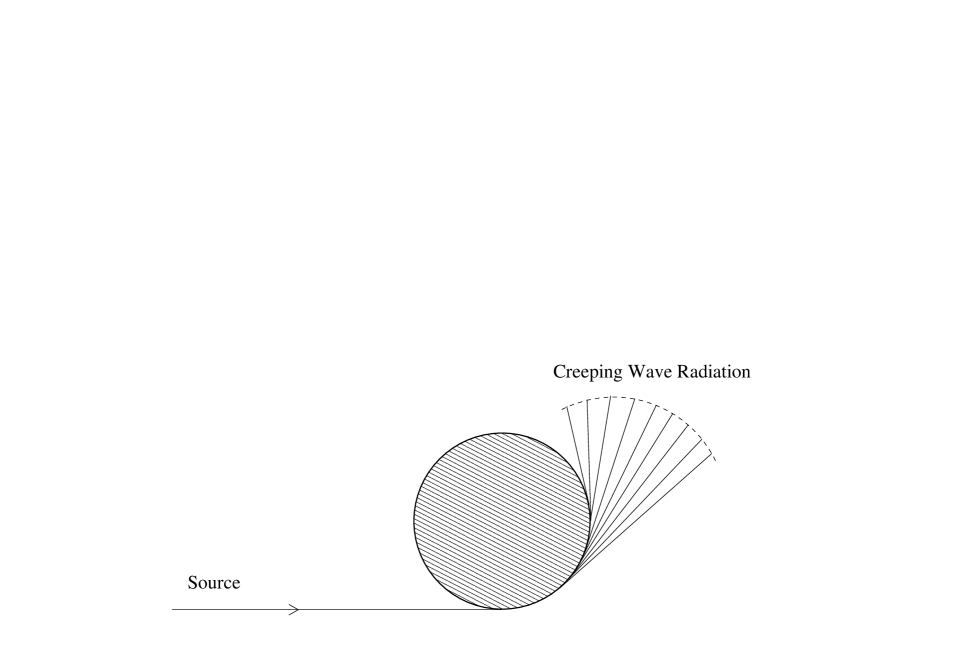
Figure 1: Geometric representation of the propagation of the creeping waves into the shadow of a spherical obstacle.

The surface of the diffracting body is the envelope of the diffracted rays: it is a caustic and, consequently, the classical method of the stationary phase fails on it. By using a modified method of the stationary phase, due to Chester, Friedman and Ursell [12], we derive a countably infinite set of factors which describe the damping of the creeping waves along the surface: these damping factors depend on the obstacle curvature. These results, which lead to the Ludwig–Kravtsov [13, 14] uniform expansion at the caustic, are briefly discussed in subsection 3.2.

From these introductory considerations the following geometrical ingredients emerge:

1. the non-uniqueness of the Cauchy problem at the boundary of the manifold in a Riemannian obstacle problem;

2. the correspondence between the homotopy classes of the fundamental group of the circle and the number of crossings through the axial caustic;

3. the Maslov phase-shift associated with the crossing-number of the ray;

4. the relationship between the curvature of the obstacle and the damping of the creeping waves along the surface of the obstacle.

In Section 3 a theory of the surface waves generated by diffraction, that makes use of these geometrical properties, is presented. Throughout this work we keep, as a typical example, the diffraction of the light by a convex and opaque object, and, for the sake of simplicity, the light is represented as a scalar. By using the same method, analogous results can be obtained in sound diffraction (see the spectacular examples of creeping waves in acoustic diffraction in Ref. [15]) and, presumably, also in the diffraction of nuclear particles [16].

A considerable part of the results that we obtain can be proved in a quite general geometrical setting: this is the case, for instance, of the proof of the existence of the diffracted rays, which derives solely from the non-uniqueness of the Cauchy problem. But, for other results, we have to restrict the class of obstacles to the surfaces of Besse type: i.e. the manifolds all of whose geodesics are closed [17]. In particular, the sphere is a Besse surface. In this case all the results obtained by geometrical methods can be easily compared with those obtained by using standard methods based on the expansion of the amplitude in series (see subsection 3.3). When the obstacle radius is large, compared to the wavelength, the series converge very slowly, and the standard procedure suggests the use of the Watson resummation [18, 19]. However, these formal manipulations do not shed light on the actual physical process. Then, the geometrical approach is expected to be very useful in the investigation of more refined features, like ripples [20], which are very sensitive to initial conditions and size parameters.

Finally, notice that our analysis will be limited to the geometrical theory of surface waves, whose effects are dominant in a small backward angular region, as it will be explained in subsection 3.3. The reader interested to a detailed analysis of which effect is dominant in the various angular domains, and, accordingly, to a systematic discussion of the transition regions, is referred to Ref. [20] (in particular, Chapter 7 and Fig. 7.7).

2 Riemannian Geometrical Optics

2.1 Non-Uniqueness of Cauchy Problem in the Riemannian Manifold with Boundary: the Diffracted Rays

In the variational derivation of geometrical optics, in particular for the laws of reflection and refraction, use is made of the Fermat’s principle: the paths of the reflected or refracted rays are stationary in the class of all the paths that touch the boundary between two media at one point, assumed to be an interior boundary point. To introduce the paths of the diffracted rays it is required a generalization of the Fermat’s principle, extended to include points, as well as arcs, lying on the boundary [20]. In our analysis, instead of the Fermat’s, we use the Jacobi form of the principle of least action [21] which concerns with the path of the system point rather than with its motion in time. More precisely, the Jacobi principle states: if there are no forces acting on the body, then the system point travels along the shortest path length in the configuration space. Moving from mechanics to optics, Riemannian geometrical optics can be rested on the Jacobi principle, formulated as follows: the light rays travel along geodesics.

In this context the diffraction by a convex, smooth and opaque object can be reconsidered as a Riemannian obstacle problem: the object is regarded as an obstacle which a geodesic can bend around, or which a geodesic can end at. Let ${\mathord{\mathbb{K}}}$ denote the obstacle which is embedded in a complete $n$-dimensional Riemannian manifold $({\mathord{\mathbb{H}}},g)$, where $g$ is the metric of ${\mathord{\mathbb{H}}}$ and $n\geq 3$. Let us introduce the space ${\mathord{\mathbb{M}}}={\mathord{\mathbb{H}}}\backslash\overline{{\mathord{\mathbb{K}}}}$, where the obstacle ${\mathord{\mathbb{K}}}$ is an open connected subset of ${\mathord{\mathbb{H}}}$, with regular boundary $\partial{\mathord{\mathbb{K}}}$ and compact closure $\overline{{\mathord{\mathbb{K}}}}={\mathord{\mathbb{K}}}\cup\partial{\mathord{\mathbb{K}}}$. Although most of the results illustrated below hold true in a very general setting, in the following we keep very often, as a typical example, ${\mathord{\mathbb{H}}}\equiv{\mathord{\mathbb{R}}}^{3}$ endowed with the euclidean metric. Finally, we are led to consider the space ${\mathord{\mathbb{M}}}^{*}={\mathord{\mathbb{M}}}\cup\partial{\mathord{\mathbb{K}}}\left(={\mathord{\mathbb{H}}}\backslash{\mathord{\mathbb{K}}}\right)$, that has the structure of a manifold with boundary.

Now, two kinds of difficulties arise: the first one concerns geodesic completeness, that is the possibility to extend every geodesic infinitely and in a unique way; this uniqueness is indeed missing in ${\mathord{\mathbb{M}}}^{*}$ at the points of the boundary. The second difficulty is related to the necessity of finding suitable coordinates at the boundary which allow for using the ordinary tools of the differential geometry, e.g. for writing the equations of the geodesics.

Concerning the first point, the lack of geodesic completeness can be treated by introducing the notion of geodesic terminal (see Ref. [22]) to represent a point where a geodesic stops. Following Plaut [22], it can be proved that ${\mathord{\mathbb{M}}}^{*}$ is the completion of ${\mathord{\mathbb{M}}}$ by observing that the set ${\cal I}$ of the geodesic terminals is nowhere dense and $\partial{\mathord{\mathbb{M}}}^{*}=\partial{\mathord{\mathbb{K}}}={\cal I}$.

Regarding the second point, it is convenient to model the manifold with boundary on the half–space ${\mathord{\mathbb{R}}}^{n}_{+}=\left\{(x_{1},...,x_{n})\in{\mathord{\mathbb{R}}}^{n}|x_{n}\geq 0\right\}\subset{\mathord{\mathbb{R}}}^{n}$, where ${\mathord{\mathbb{R}}}^{n-1}_{0}$ denotes the boundary $x_{n}=0$ of ${\mathord{\mathbb{R}}}^{n}_{+}$. Thus, for a manifold with boundary, there exists an atlas $\{{\cal U}^{\alpha}\}$, with local coordinates $(x_{1}^{\alpha},...,x_{n}^{\alpha})$, such that in any chart we have the strict inequality $x^{\alpha}_{n}>0$ at the interior points, and $x^{\alpha}_{n}=0$ at the boundary points. The set $\partial{\mathord{\mathbb{M}}}^{*}$ of the boundary points is a smooth manifold of dimension $(n-1)$.

In a Riemannian manifold without boundary, the geodesics are the solutions of a system of differential equations with suitable Cauchy conditions. The main result is the theorem which guarantees existence, uniqueness and smoothness of the solution for the Cauchy problem of this system. The case of Riemannian manifold with boundary is different from the classical one for what concerns uniqueness and smoothness of the solutions.

In order to write the equation of a geodesic $\gamma$ of ${\mathord{\mathbb{M}}}^{*}$, we introduce suitable coordinates $x_{i}$ $(i=1,\ldots,n)$ adapted to the boundary, called geodesic boundary coordinates [6, 7], with $x_{n}$ defined as the distance from the boundary $\partial{\mathord{\mathbb{M}}}^{*}$; then starting with arbitrary coordinates $x_{i},~{}i<n$ on $\partial{\mathord{\mathbb{M}}}^{*}$, we extend them to be constant on ordinary geodesics normal to $\partial{\mathord{\mathbb{M}}}^{*}$. Let $\Gamma_{ijk}$ denote the Christoffel symbols of the Levi Civita connection of ${\mathord{\mathbb{M}}}^{*}$, and $\chi$ be the normal curvature of $\partial{\mathord{\mathbb{M}}}^{*}$ in the direction of $\gamma$. Then, we have:

$$\chi=-\sum_{i,j<n}\dot{x}_{i}\,\dot{x}_{j}\,\Gamma_{ijn}.$$ (1)

When $\gamma$ is not in $\partial{\mathord{\mathbb{M}}}^{*}$ the same expression occurs in the differential equations for $\gamma$, so that if we define $\chi=0$ off the boundary segments, then the differential equations can be modified to cover, in an integral sense, all points of $\gamma$, as follows [6, 7]:

$$\displaystyle\ddot{x}_{k} = -\sum_{i,j}\dot{x}_{i}\,\dot{x}_{j}\,\Gamma_{ijk},~{}~{}~{}~{}~{}(k<n),$$ (2)

$$\displaystyle\ddot{x}_{n} = -\chi-\sum_{i,j<n}\dot{x}_{i}\,\dot{x}_{j}\,\Gamma_{ijn}.$$ (3)

Equations (2, 3) can be implemented with the Cauchy conditions by providing the values of ${\bf x}(t)$ and $\dot{{\bf x}}(t)\,\,({\bf x}\equiv(x_{1},...,x_{n}))$ when $t=0$:

$$x_{i}(0) = b_{i},~{}~{}~{}~{}~{}(i<n),~{}~{}~{}x_{n}(0)=0,$$ (4)

$$\dot{x}_{i}(0) = v_{i},~{}~{}~{}~{}~{}(i<n),~{}~{}~{}\dot{x}_{n}(0)=0,$$ (5)

where $(b_{1},...,b_{n})$ are the coordinates of the point $b$ belonging to the boundary, and $(v_{1},...,v_{n})$ are the components of the tangent vector at $b$.

Now, let us consider the following cases:

1. $x_{n}\equiv 0$. In view of equalities (1) and (3), we remain with system (2) composed by $(n-1)$ differential equations that describe a geodesic on the $(n-1)$ dimensional smooth manifold $\partial{\mathord{\mathbb{M}}}^{*}$ (i.e. $x_{n}=0$), which is a manifold without boundary. In this case the standard theorem on the existence, uniqueness and smoothness of the geodesics satisfying the given Cauchy conditions holds true. We have a $C^{\infty}$-class geodesic which is completely contained on the boundary.

2. $x_{n}(t)=0$ if $t\leq 0$, and $x_{n}(t)>0$ if $t>0$. In view of the fact that $\chi=0$ off the boundary segments, eqs. (2, 3) describe, for $t>0$, a geodesic segment belonging to the interior of ${\mathord{\mathbb{M}}}^{*}$ (i.e. $\stackrel{{\scriptstyle\scriptscriptstyle\circ}}{{{\mathord{\mathbb{M}}}^{*}}}$). Moreover, eqs. (2, 3) describe, for $t<0$, a geodesic segment belonging to the boundary. Notice that the r.h.s. of (2) is continuous, so that (2) holds everywhere as it is. If $\chi\neq 0$ on boundary segments, from Eq. (3) it can be easily seen that $\ddot{x}_{n}$ fails to be continuous at the point $b$ $(t=0)$. Nevertheless, in view of the Cauchy conditions (i.e. $x_{n}(0)=\dot{x}_{n}(0)=0$), the two geodesic segments (one belonging to the boundary, the other belonging to the interior of ${\mathord{\mathbb{M}}}^{*}$) glue necessarily at $b$, and give rise to a geodesic of ${\mathord{\mathbb{M}}}^{*}$ of class $C^{1}$ at the transitions point $b$.

3. $x_{n}(t)=0$, if $t\geq 0$, $x_{n}(t)>0$ if $t<0$. The analysis is analogous to the previous one at point (b). We can say that two geodesic segments (one belonging to the interior of ${\mathord{\mathbb{M}}}^{*}$, the other one to the boundary) glue together at $b$ and give rise to a geodesic of ${\mathord{\mathbb{M}}}^{*}$ of class $C^{1}$ at the transition point $b$.

4. $x_{n}(t)=0$ if and only if $t=0$. Following considerations strictly analogous to those developed above, we can say that eqs. (2, 3) describes two geodesic segments which belong to the interior of ${\mathord{\mathbb{M}}}^{*}$, and have only one point of contact with the boundary at $b$. Therefore, gluing at $b$ the two geodesic segments, we obtain a geodesic of ${\mathord{\mathbb{M}}}^{*}$ of class $C^{\infty}$.

Since we supposed the obstacle to be compact with smooth and convex boundary, the analysis performed above is exhaustive.

Summarizing, if $\chi\neq 0$ on the boundary segments, we can glue together, at the point $b\in\partial{\mathord{\mathbb{M}}}^{*}$, a geodesic segment belonging to the boundary with a geodesic segment belonging to the interior of ${\mathord{\mathbb{M}}}^{*}$ (cases (b) and (c)), and, in these case, we have a geodesic of ${\mathord{\mathbb{M}}}^{*}$, which is of class $C^{1}$ at the transition point $b$. Thus, we have obtained the diffracted rays, which are precisely the geodesics of ${\mathord{\mathbb{M}}}^{*}$ of this type. The situation considered in case (d) is of minor interest for our analysis, since those geodesics correspond to rays which are not diffracted even if they touch the obstacle.

As a consequence of the non-uniqueness of the Cauchy problem at the boundary of the manifold, that can be made transparent by the use of equations (2) and (3), we can conclude by saying that at each point of the boundary we have a bifurcation: the ray splits in two, one part continues as an ordinary ray (diffracted ray of class $C^{1}$ at the splitting point), the other part travels along the surface as a geodesic of the boundary.

Finally, let us observe that the contact point $b$ on the boundary is necessarily an elliptic point in view of the assumptions of convexity and compactness made about the obstacle.

2.2 Conjugate Points (Axial Caustic) and Morse theorem in a Riemannian Manifold with Boundary

First, let us consider a complete Riemannian manifold ${\mathord{\mathbb{M}}}$ without boundary. Given a geodesic $\gamma=\gamma(t)$, $0\leq t\leq 1$, consider a geodesic variation of $\gamma$, that is a one-parameter family of geodesics $\gamma_{s}=\gamma_{s}(t)$, $(-\epsilon<s<\epsilon)$ such that $\gamma_{0}=\gamma$. For each fixed $s$, $\gamma_{s}(t)$ describes a geodesic when $t$ varies from $0$ to $1$. Each variation gives rise to an infinitesimal variation, that is, a certain vector field defined along $\gamma$. The points $\gamma(0)$ and $\gamma(1)$ of $\gamma$ are said to be conjugate if there is a variation $\gamma_{s}$ which induces an infinitesimal variation vanishing at $t=0$ and $t=1$ (see Ref. [23]).

Set $f(s,t)=\gamma_{s}(t)$, and denote by $D/{\partial t}$ and $D/{\partial s}$ the covariant differentiation with respect to $t$ and $s$, respectively. Denote by $R$ the curvature transformation determined by $\partial f/\partial t$ and $\partial f/\partial s$, i.e.

$$R\left(\frac{\partial f}{\partial t},\frac{\partial f}{\partial s}\right)\frac{\partial f}{\partial t}=\left(\frac{D}{\partial s}\,\frac{D}{\partial t}-\frac{D}{\partial t}\,\frac{D}{\partial s}\right)\frac{\partial f}{\partial t}.$$ (6)

A vector field $Y$ is a Jacobi field along $\gamma$ if satisfies the following differential equation:

$$J\,Y\equiv Y^{{}^{\prime\prime}}+R\,(\gamma^{{}^{\prime}},Y)\,\gamma^{{}^{\prime}}=0,$$ (7)

where $\gamma^{{}^{\prime}}\equiv d\gamma/dt$, $Y^{{}^{\prime\prime}}$ is the second covariant derivative of $Y$ along $\gamma$, and $R\,(\gamma^{{}^{\prime}},Y)$ is the curvature transformation defined by equality (6). Two points $p,q\in{\mathord{\mathbb{M}}}$ are conjugate along $\gamma$ if there exists a non-trivial Jacobi field $Y$ along $\gamma$ such that $Y(p)=Y(q)=0$. Finally, the multiplicity of the pair of conjugate points $p,q\in\gamma$ is given by the dimension of the vector space of the linearly independent Jacobi fields, along $\gamma$, that vanish at $p$ and $q$.

Let us now introduce the infinite dimensional space $\Omega({\mathord{\mathbb{M}}};p,q)$ of piecewise differentiable paths $c$ connecting on ${\mathord{\mathbb{M}}}$ the point $p$ with the point $q$: i.e. let $p$ and $q$ be two fixed points on ${\mathord{\mathbb{M}}}$, and $c:[0,1]\rightarrow{\mathord{\mathbb{M}}}$ be a piecewise differentiable path such that $c\,(0)=p$, $c\,(1)=q$. To any element $c\in\Omega({\mathord{\mathbb{M}}};p,q)$ we associate an infinite dimensional vector space $T_{c}\Omega$, which can be identified with the space tangent to $\Omega$ in a point $c$. More precisely $T_{c}\Omega$ is the vector space composed by all those fields of piecewise differentiable vectors $V$ along the path $c$, such that $V(0)=0$, $V(1)=0$. Next, we introduce the energy-functional

$$E(c)=\int_{0}^{1}\>\left|\frac{dc}{dt}\right|^{2}\,dt=\int_{0}^{1}\,g_{ij}\,\dot{x}^{i}\,\dot{x}^{j}\,dt,$$ (8)

where $g_{ij}$ is the metric of ${\mathord{\mathbb{M}}}$, and $(x^{1},....,x^{n})$ are local coordinates on ${\mathord{\mathbb{M}}}$. From the first variation of functional $E$ we can deduce that the extremals of functional $E(c)$ are represented by the geodesics $c\,(t)=\gamma(t)$, parametrized by $t$. Let us now consider the second variation $E_{**}$ of the functional $E$ along the geodesic $\gamma$ (it will be called the hessian of $E$), and let $\lambda$ be the index of the hessian, that is the largest dimension of the subspace of $T_{\gamma}\Omega$ on which $E_{**}$ is definite negative. One can then state the following Theorem:

Theorem 1

(Morse Index Theorem [9]) The index $\lambda$ of the hessian $E_{**}$ equals the number of points belonging to $\gamma(t)$ which are conjugate to the initial point $p=\gamma(0)$, each one counted with its multiplicity.

Now let us go back to our main concern, the Riemannian manifold with boundary ${\mathord{\mathbb{M}}}^{*}$. Following Alexander [24], we define as a Jacobi field any vector field $Y$ along the geodesic $\gamma$ (whose boundary contact intervals have positive measure), which satisfies the following conditions: $Y$ is continuous, it is a Jacobi field of both $\stackrel{{\scriptstyle\scriptscriptstyle\circ}}{{{\mathord{\mathbb{M}}}^{*}}}$ and $\partial{\mathord{\mathbb{M}}}^{*}$ along every segment of $\gamma$, and at each endpoint $t_{i}$ of a contact interval it satisfies the following equation:

$$P\left(\frac{D}{\partial t}\,Y\right)(t_{i}^{-})=P\left(\frac{D}{\partial t}\,Y\right)(t_{i}^{+}),$$ (9)

where $P$ denotes orthogonal projections onto the hyperplane tangent to $\partial{\mathord{\mathbb{M}}}^{*}$. In the Riemannian manifold with boundary we are forced to consider geodesics which lie both on and off $\partial{\mathord{\mathbb{M}}}^{*}$, and that are merely $C^{1}$ at the transition points (see the previous subsection). However, it is still possible to define a hessian form which is given simply by the sum of the classical formulae for $\partial{\mathord{\mathbb{M}}}^{*}$ on contact intervals, and for the interior of ${\mathord{\mathbb{M}}}^{*}$ (i.e. $\stackrel{{\scriptstyle\scriptscriptstyle\circ}}{{{\mathord{\mathbb{M}}}^{*}}}$) on interior intervals. Furthermore, we call $\gamma(0)$ and $\gamma(1)$ conjugate if there is a non trivial Jacobi field $Y$ along $\gamma$ whose limits at the endpoints vanish. Finally, the Morse index theorem can be extended to the Riemannian manifold with boundary. To this purpose, it is convenient to introduce the so-called regular geodesics in the sense of Alexander. Following Ref. [24], a geodesic $\gamma$ is regular if:

1. all boundary-contact intervals of $\gamma(t)$ have positive measure;

2. the points of arrival of $\gamma(t)$ at $\partial{\mathord{\mathbb{M}}}^{*}$ are not conjugate to the initial point $\gamma(0)$.

Then we can formulate the extended Morse index theorem as follows:

Theorem 2 (Morse Index Theorem for Riemannian Manifolds with Boundary [24])

Let $\gamma$ be a regular geodesic; then the index $\lambda$ of $E_{**}$ is finite and equal to the number of points belonging to $\gamma(t)$ conjugate to the initial point $\gamma(0)$ ($0\leq t\leq 1$), counted with their multiplicities.

It still remains to check if the diffracted rays are regular geodesics. First of all we suppose that the source of light is located in a point $p_{0}\in\stackrel{{\scriptstyle\scriptscriptstyle\circ}}{{{\mathord{\mathbb{M}}}^{*}}}$ (point source); then the diffracted rays which we are considering connect the point $p_{0}$ and a point $q\in\stackrel{{\scriptstyle\scriptscriptstyle\circ}}{{{\mathord{\mathbb{M}}}^{*}}}$, placed at the exterior to the obstacle. If we assume that ${\mathord{\mathbb{H}}}={\mathord{\mathbb{R}}}^{3}$ (equipped with euclidean metric), then the diffracted rays consist of a straight line segment from $p_{0}$ to the body surface, of a geodesic along the surface, and a straight line segment from the body to $q$. Now, in view of the fact that these rays undergo diffraction, they cannot be simply tangent to the obstacle, but the contact-interval must be a geodesic segment of positive measure. Therefore condition (a) is satisfied. Concerning condition (b), we simply note that it is certainly satisfied in view of the fact that we consider obstacles formed by a convex and compact body embedded in ${\mathord{\mathbb{R}}}^{3}$, and the latter does not have conjugate points.

2.3 Morse Index and Homotopy Classes of Diffracted Rays

Hereafter the analysis will be limited to obstacles represented by manifolds all of whose geodesics are closed (i.e. Besse manifolds [17]). Merely for the sake of simplicity, henceforth we shall consider as obstacles spherical balls embedded in ${\mathord{\mathbb{R}}}^{3}$: i.e $\partial{\mathord{\mathbb{K}}}\equiv S^{2}$, equipped with standard metric. However, in view of the homotopic invariance, the main result of this section (see next (10, 11)) holds true for any convex and compact Besse type manifold.
Consider the axis of symmetry $A$ of the obstacle ${\mathord{\mathbb{K}}}$ passing through the point $p_{0}\in\stackrel{{\scriptstyle\scriptscriptstyle\circ}}{{{\mathord{\mathbb{M}}}^{*}}}$, where it is located the source of light, and denote by $A_{-}$ the portion of this axis lying in the illuminated region (i.e. the same side of the light source), and by $A_{+}$ the portion of the axis lying in the shadow. The axis $A$ equals $A_{-}\cup D\cup A_{+}$, where $D$ is the diameter of the sphere. Let us note that all the points of ${\mathord{\mathbb{M}}}^{*}$ that do not belong to $A_{+}$ are connected to $p_{0}$ by only one geodesic of minimal length, whereas the points $q\in A_{+}$ are connected to $p_{0}$ by a continuum of geodesics of minimal length that can be obtained as the intersections of ${\mathord{\mathbb{M}}}^{*}$ with planes passing through the axis $A$. By rotating these planes, and keeping $p_{0}$ and $q\in A_{+}$ fixed, we obtain a variation vector field which is a Jacobi field vanishing at $p_{0}$ and $q$. Thus, we can conclude that $p_{0}$ and $q\in A_{+}$ are conjugate with multiplicity one because the possible rotations are only along one direction. Then, in view of the extended form of the Morse Index Theorem, we can state that the index $\lambda$ of $E_{**}$ jumps by one when the geodesic $\gamma(t)$, whose initial point is $\gamma(0)=p_{0}$, crosses $A_{+}$.

Now let us focus our attention on the points $q\in{\mathord{\mathbb{M}}}^{*}\backslash(A_{+}\cup A_{-})$ (i.e. which do not lie on the axis of the obstacle, see Fig. 2). Consider the space $X_{p_{0}q}=({\mathord{\mathbb{E}}}^{2})_{q}\cap{\mathord{\mathbb{M}}}^{*}$, where $({\mathord{\mathbb{E}}}^{2})_{q}$ is the plane uniquely determined by the axis of the obstacle through $p_{0}$ and the point $q$. $X_{p_{0}q}$ (which will be denoted hereafter simply by $X$) is an arcwise connected space, whose boundary in $({\mathord{\mathbb{E}}}^{2})_{q}$ is a circle $S$ which is a deformation retract of $X$. In view of these facts the fundamental group $\pi_{1}(X;p_{0})$ does not depend on the base point $p_{0}$ and is isomorphic to $\pi_{1}(S^{1};{\bf 1})$, where ${\bf 1}$, described in a convenient system by the coordinates $(0,1)$ (see Fig. 2), represents the contact point of $A_{+}$ with $S^{2}$: $\pi_{1}(X;p_{0})\simeq\pi_{1}(S^{1};{\bf 1})\simeq{\mathord{\mathbb{Z}}}$. Let us consider, within the fundamental groupoid $\Pi_{1}(X)$ of $X$, the set $\Pi_{1}(X;p_{0},q)$ of paths in $X$ connecting $p_{0}$ with $q$, modulo homotopy with fixed end-points. We can then formulate the following statements:

Figure 2: Geometry of the problem in the case of spherical obstacle. $\gamma_{0}$ is the unique geodesic of minimal length when the point $q$ does not belong to the axial caustic (the $z$-axis). $\alpha_{0}$ is a counterclockwise loop at $p_{0}$.

Proposition 1

Each element of $\pi_{1}(X;p_{0})$ is a homotopy class $[\alpha]$, with fixed endpoints, of a certain loop $\alpha:[0,1]\rightarrow X$, in the space $X$, starting and ending at the point $p_{0}$.

Proposition 2

Each path $c_{0}$ from $p_{0}$ to $q\in{\mathord{\mathbb{M}}}^{*}\backslash(A_{+}\cup A_{-})$, determines a one-to-one correspondence $W$ between $\pi_{1}(X;p_{0})$ and the set $\Pi_{1}(X;p_{0},q)$. Such a correspondence can be constructed as: $\forall\,[c]\in\Pi_{1}(X;p_{0},q):[c]\longrightarrow[c\star c_{0}^{-1}]\in\pi_{1}(X;p_{0})$, where the symbol ’$\star$’ denotes the concatenation of paths, and $c_{0}^{-1}$ denotes the reverse path of $c_{0}$.

Proposition 3

i) In each homotopy class of $\pi_{1}(X;p_{0})$ there is precisely one element of minimal length. ii) In each homotopy class of $\Pi_{1}(X;p_{0},q)$, $q\in{\mathord{\mathbb{M}}}^{*}\backslash(A_{+}\cup A_{-})$, there is precisely one geodesic.

Because of Propositions 2 and 3 we can establish a bijective correspondence $w$ between geodesics from $p_{0}$ to $q$ (fixed) and integral numbers. Let us make precise our choices:

1. $q$ is fixed in $X\backslash(A_{+}\cup A_{-})$; we introduce in $({\mathord{\mathbb{E}}}^{2})_{q}$ a reference system so that $p_{0}$ belongs to the negative part of the $z$-axis, and the value of the coordinate $x$ of the point $q$ (i.e. $x_{q}$) is positive (see Fig. 2);

2. $\gamma_{0}$ is the geodesic from $p_{0}$ to $q$ of minimal length;

3. $\alpha_{0}$ is a loop in $X$ at $p_{0}$, such that:

   1. $[\alpha_{0}]$ is a generator of $\pi_{1}(X;p_{0})$ (establishing an isomorphism $\pi_{1}(X;p_{0})\simeq{\mathord{\mathbb{Z}}}$);

   2. $\alpha_{0}$ turns in counterclockwise sense around the obstacle (see Fig. 2).

Now, the correspondence $w$ maps the geodesic $\gamma$ into the number $w(\gamma)$ such that $[\gamma\star\gamma_{0}^{-1}]=w(\gamma)\,[\alpha_{0}]$. Note that $w(\gamma)$ is the winding number of the loop $[\gamma\star\gamma_{0}^{-1}]$ determined by $\gamma$ (with respect to the chosen generator $[\alpha_{0}]$).

We can also characterize the geodesics (from $p_{0}$ to $q$) by a natural number $n(\gamma)$, which we call the crossing-number of $\gamma$, having a clearer geometric interpretation: $n(\gamma)$ counts the number of crossings of $\gamma$ across the $z$-axis. For instance, $n(\gamma_{0})=0$. It is easy to see that the winding number determines the crossing-number through the following bijective correspondence:

$${\mathord{\mathbb{Z}}} ~{}~{}~{}\longrightarrow~{}~{}~{} \hskip 14.22636pt{\mathord{\mathbb{N}}}$$

$$m ~{}~{}~{}\longrightarrow~{}~{}~{} (2m-1)~{}~{}~{}~{}~{}~{}~{}~{}(m>0)$$ (10)

$$m ~{}~{}~{}\longrightarrow~{}~{}~{} \hskip 7.11317pt-2m\,~{}~{}~{}~{}~{}~{}~{}~{}~{}~{}~{}(m\leq 0)$$ (11)

so that our previous statement on the bijective correspondence between the geodesics and their crossing-number is established.

3 Surface Waves in Diffractive Scattering

3.1 Creeping Waves on the Sphere

In this subsection we consider a Riemannian manifold without boundary ${\mathord{\mathbb{M}}}^{n}$; $\Omega$ is a chart of ${\mathord{\mathbb{M}}}^{n}$, ${\bf x}=(x_{1},...,x_{n})$ are the local coordinates in $\Omega$ and $g_{ij}({\bf x})$ is the metric tensor. As usual $g=|\mbox{det\,}(g_{ij})|$ and $g^{ij}=g_{ij}^{-1}$. Let us consider the Helmholtz equation

$$\Delta_{2}u+k^{2}u=0,$$ (12)

where $\Delta_{2}$ is the Laplace-Beltrami operator which, for a function $u\in C^{\infty}({\mathord{\mathbb{M}}}^{n})$, reads

$$\Delta_{2}u=\frac{1}{\sqrt{g}}\,\sum_{i=1}^{n}\,\frac{\partial}{\partial x_{i}}\left(\sum_{j=1}^{n}g^{ij}\,\sqrt{g}\,\frac{\partial}{\partial x_{j}}\right)u.$$ (13)

Now, we look for a solution of Eq. (12) of the following form:

$$u({\bf x},k)=\int A({\bf x},\beta)~{}e^{ik\Phi({\bf x},\beta)}~{}d\beta.$$ (14)

The principal contribution to $u({\bf x},k)$, as $k\rightarrow+\infty$, corresponds to the stationary points of $\Phi$, in the neighbourhoods of which the exponential $e^{ik\Phi}$ ceases to oscillate rapidly. These stationary points can be obtained from the equation $\partial\Phi({\bf x},\beta)/\partial\beta=0$ (provided that $\partial^{2}\Phi/\partial\beta^{2}\neq 0$). Let us now suppose that for each point ${\bf x}=(x_{1},...,x_{n})$ $\Phi$ has only one stationary point; then the following asymptotic expansion of $u$, as $k\rightarrow\infty$, is valid [10]:

$$u({\bf x},k)\,\simeq\,e^{ik\Phi({\bf x},\beta_{0})}\sum_{m=0}^{\infty}\frac{A_{m}}{(ik)^{m}},$$ (15)

where $\beta_{0}$ is the unique stationary point of $\Phi$. The leading term of expansion (15) is:

$$u({\bf x},k)=A_{0}({\bf x})\,e^{ik\Phi({\bf x},\beta_{0})},$$ (16)

where

$$A_{0}({\bf x})=A({\bf x},\beta_{0})\left(\left|\frac{\partial^{2}\Phi}{\partial\beta^{2}}\right|^{-\frac{1}{2}}\right)_{\!\!\beta=\beta_{0}}\exp\left\{{i\,\frac{\pi}{4}{\,\,\mbox{sgn\,}}\left(\frac{\partial^{2}\Phi}{\partial\beta^{2}}\right)_{\!\beta=\beta_{0}}}\right\}.$$ (17)

By substituting the leading term (which will be written hereafter as $A\exp\{ik\Phi\}$, omitting the index zero) into equation (12), collecting the powers of $(ik)$, and, finally, equating to zero their coefficients, two equations are obtained: the eikonal (or Hamilton-Jacobi) equation

$$g^{ij}\frac{\partial\Phi}{\partial x_{i}}\,\frac{\partial\Phi}{\partial x_{j}}=1,$$ (18)

and the transport equation

$$\frac{1}{\sqrt{g}}\,\sum_{i=1}^{n}\frac{\partial}{\partial x_{i}}\left\{\sqrt{g}\left(A^{2}\sum_{j=1}^{n}g^{ij}\,\frac{\partial\Phi}{\partial x_{j}}\right)\right\}=0,$$ (19)

whose physical meaning is the conservation of the current density.

We can switch from wave to ray description by writing the eikonal equation in the form of a Hamilton-like system of differential equations by setting

$$\displaystyle p_{i} = \frac{\partial\Phi}{\partial x_{i}},$$ (20)

$$\displaystyle F = \frac{1}{2}\left(g^{ij}\,p_{i}\,p_{j}-1\right),$$ (21)

and obtaining the characteristic system

$$\displaystyle\frac{dx_{i}}{d\tau} = g^{ij}\,p_{j},$$ (22)

$$\displaystyle\frac{dp_{i}}{d\tau} = -\frac{\partial F}{\partial x_{i}}=-\frac{1}{2}\>p_{i}\,p_{j}\,\frac{\partial g^{ij}}{\partial x_{i}},$$ (23)

where $\tau$ is a running parameter along the ray emerging from the surface $\Phi=$ const.

Whenever the amplitude $A$ becomes infinite, approximation (16) fails, and, consequently, such an approximation holds true only locally. Thus, we are faced with the problem of passing from a local to a global approximation, i.e. a solution in the whole space. The strategy for constructing a solution in the whole space consists in patching up local solutions by means of the so called Maslov-indexes in a way that will be illustrated below in the specific case of ${\mathord{\mathbb{M}}}^{n}=S^{2}$.

Let the unit sphere be described by the angular coordinates $\theta$ and $\phi$. The matrix elements $g_{ij}$ have the following values: $g_{11}=1$, $g_{22}=\sin^{2}\theta$, $g_{12}=g_{21}=0$. In addition, we assume that the phase $\Phi$ and the amplitude $A$ do not depend on the angle $\phi$. Then, eqs. (18) and (19) become, respectively

$$\left(\frac{d\Phi}{d\theta}\right)^{2}=1,$$ (24)

$$\frac{1}{|\sin\theta|}\left\{\frac{d}{d\theta}\left(|\sin\theta|\>A^{2}\>\frac{d\Phi}{d\theta}\right)\right\}=0,~{}~{}~{}~{}~{}\theta\neq n\pi.$$ (25)

From Eq. (24) we have: $\Phi=\pm\theta+\mbox{const.\,}$, and from Eq. (25) we obtain: $A\,(\theta)=\mbox{const.\,}\cdot|\sin\theta|^{-1/2},\,\theta\neq n\pi$. Therefore, approximation (16) becomes

$$u\,(\theta,k)=\frac{\mbox{const.\,}}{\sqrt{|\sin\theta|}}~{}e^{\pm ik\theta},~{}~{}~{}~{}~{}~{}~{}~{}~{}\theta\neq n\pi,$$ (26)

where the terms $\exp\{\pm ik\theta\}$ represent waves traveling counterclockwise ($\exp\{ik\theta\}$) or clockwise ($\exp\{-ik\theta\}$) around the unit sphere. Since the approximation (26) fails at $\theta=n\pi$, ($n=0,1,2...$), we have to consider the problem of patching these approximations when the surface rays cross the antipodal points $\theta=0,\pi$, which are conjugate points in the sense of the Morse theory (see Section 2.3). This difficulty will be overcome by the use of the Maslov construction [25, 26, 10, 11].

In order to illustrate the Maslov scheme in the case ${\mathord{\mathbb{M}}}^{n}\equiv S^{2}$, we reconsider the problem of the waves creeping around the unit sphere in a more general setting. The Hamilton-Jacobi equation (18) is rewritten in the form:

$$H=g^{ij}\,p_{i}\,p_{j}=p_{\theta}^{2}+\frac{1}{\sin^{2}\theta}\>p_{\phi}^{2}=1.$$ (27)

In order to find the first integrals $h$ of the system, we equal to zero the Poisson brackets: $\{h,H\}=0$, to get:

$$\displaystyle p_{\phi} = c_{1},$$ (28)

$$\displaystyle p_{\theta}^{2} + \frac{c_{1}^{2}}{\sin^{2}\theta}=1.$$ (29)

Furthermore, we have:

$$\Phi_{\pm}(\theta,\phi)=\int(p_{\phi}\,d\phi+p_{\theta}\,d\theta)=c_{1}\phi\pm\Phi_{1}(\theta),$$ (30)

(notice that $p_{\theta}=\pm\{1-(c_{1}^{2}/\sin^{2}\theta)\}^{1/2}$). Equation (29) defines a smooth curve in the domain $0<\theta<\pi$, $p_{\theta}\in{\mathord{\mathbb{R}}}$, which is diffeomorphic to the circle. The points where the tangent to the curve is vertical have coordinates $(\theta_{0},0)$, $(\pi-\theta_{0},0)$, with $\theta_{0}=\sin^{-1}(c_{1})$, $c_{1}>0$. The cycles of singularities are given by the equations (see Ref. [10], Fig. 16):

$$p_{\phi} = c_{1},~{}~{}p_{\theta}=0;~{}~{}~{}~{}\theta=\theta_{0},~{}~{}0\leq\phi\leq 2\pi,$$ (31)

$$p_{\phi} = c_{1},~{}~{}p_{\theta}=0;~{}~{}~{}~{}\theta=\pi-\theta_{0},~{}~{}0\leq\phi\leq 2\pi.$$ (32)

Then, the neighbourhoods of the points $\theta=\theta_{0}$ and $\theta=\pi-\theta_{0}$ are badly projected on the configuration space $(\theta,\phi)$. However, the Maslov theory guarantees that it is possible to choose other local coordinates such that the mapping from the Lagrangian manifold to the selected coordinates is locally a diffeomorphism. In the present case it is easy to see that the mapping in the plane $(p_{\theta},\phi)$ is diffeomorphic (see Fig. 16 of Ref. [10]). Once the local asymptotic solution in terms of $(p_{\theta},\phi)$ has been computed, it is possible to return to the configuration space $(\theta,\phi)$ by transforming $p_{\theta}\rightarrow\theta$ through an inverse Fourier transform $F^{-1}_{k,p_{\theta}\rightarrow\theta}$. It is indeed the asymptotic evaluation (for large values of $k$) of $F^{-1}_{k,p_{\theta}\rightarrow\theta}$, obtained again by the stationary point method, that gives rise to an additional phase-shift in the solution. In fact, the term $\exp\{i(\pi/4)\,\mbox{sgn\,}(\partial^{2}\Phi/\partial\beta^{2})\}$ of formula (17) is modified as follows. Instead of $\Phi(\theta,\phi)$, it must be considered the phase $\tilde{\Phi}(p_{\theta},\phi)$ in the mixed representation coordinate-momentum; to have the phase described in the configuration space we move back from $p_{\theta}$ to $\theta$ by means of the inverse Fourier transformation. Then, we have an exponential term of the form $\exp\{ik[\tilde{\Phi}+\theta p_{\theta}]\}$ into an integral where $\theta$ is regarded as a fixed parameter, whereas $p_{\theta}$ is the integration variable. Let $\Phi^{{}^{\prime}}=\tilde{\Phi}+\theta p_{\theta}$. The stationary point is then determined by the equality

$$\frac{\partial\Phi^{{}^{\prime}}}{\partial p_{\theta}}=\frac{\partial\tilde{\Phi}}{\partial p_{\theta}}+\theta=0,$$ (33)

and, therefore, it is given by that value of $p_{\theta}$ such that $\partial\tilde{\Phi}/\partial p_{\theta}=-\theta$. Next, we get:

$$\mbox{sgn\,}\frac{\partial^{2}\Phi^{{}^{\prime}}}{\partial p_{\theta}^{2}}=\mbox{sgn\,}\frac{\partial^{2}\tilde{\Phi}}{\partial p_{\theta}^{2}}=-\mbox{sgn\,}\frac{\partial\theta}{\partial p_{\theta}}.$$ (34)

Therefore, the additional phase factor $\exp\{-i(\pi/4)\,\mbox{sgn\,}(\partial\theta/\partial p_{\theta})\}$ emerges.

The negative inertial index of a symmetric non–degenerate $(n\times n)$ matrix ${\cal A}$, called Inerdex, is the number of negative eigenvalues of the matrix [10]. The following relationship holds [10]: $\mbox{sgn\,}{\cal A}+2\,\mbox{\,Inerdex\,}{\cal A}=n$ (where $\mbox{sgn\,}{\cal A}$ is for the signature of the quadratic form associated with the matrix ${\cal A}$). In our case we have

$$-\mbox{sgn\,}\frac{\partial\theta}{\partial p_{\theta}}=2\mbox{\,Inerdex\,}\frac{\partial\theta}{\partial p_{\theta}}-1,$$ (35)

then:

$$\exp\left\{-i\,\frac{\pi}{4}\,\mbox{sgn\,}\frac{\partial\theta}{\partial p_{\theta}}\right\}=\exp\left\{i\,\frac{\pi}{2}\,\mbox{\,Inerdex\,}\frac{\partial\theta}{\partial p_{\theta}}-i\frac{\pi}{4}\right\}.$$ (36)

We now focus our attention on the phase factor $\exp\{i\delta\}=\exp\{i\,\frac{\pi}{2}\,\mbox{\,Inerdex\,}(\frac{\partial\theta}{\partial p_{\theta}})\}$, which is the relevant term in the analysis of the crossing through the critical points. In close analogy with the Morse index which gives the dimension of the subspace on which $E_{**}$ is negative definite, and whose jumps count the increase of this dimension (see Section 2.2), here it must be evaluated the number of transitions from positive to negative values of $(\partial\theta/\partial p_{\theta})$, or vice-versa. With this in mind, we cover the curve: $p_{\theta}^{2}+(c_{1}^{2}/\sin^{2}\theta)=1$, diffeomorphic to a circle, with four charts: let ${\cal U}^{1}$ be the chart which lies in the half-plane $p_{\theta}<0$, ${\cal U}^{3}$ be the chart which lies in the half-plane $p_{\theta}>0$, and ${\cal U}^{2}$ and ${\cal U}^{4}$ be the charts which lie in the neighbourhoods of the points $(\theta_{0},0)$ and $(\pi-\theta_{0},0)$, respectively. Next, the evaluation of $(\partial\theta/\partial p_{\theta})$ gives

$$\frac{\partial\theta}{\partial p_{\theta}}=\frac{c_{1}p_{\theta}}{(1-p_{\theta}^{2})\sqrt{1-(p_{\theta}^{2}+c_{1}^{2})}},~{}~{}~{}~{}(0<c_{1}<1).$$ (37)

Let us consider a path $l$, counterclockwise oriented, which connects two points $r^{\prime}$ and $r^{\prime\prime}$ belonging to ${\cal U}^{1}$ and ${\cal U}^{3}$, respectively. The Maslov index $\mbox{Ind\,}(l)$, defined as the variation of $\mbox{\,Inerdex\,}(\partial\theta/\partial p_{\theta})$ along $l$, reads

$$\mbox{Ind\,}(l)=\mbox{\,Inerdex\,}\left(\frac{\partial\theta}{\partial p_{\theta}}\right)_{\!\!r^{\prime\prime}}-\mbox{\,Inerdex\,}\left(\frac{\partial\theta}{\partial p_{\theta}}\right)_{\!\!r^{\prime}}=-1,$$ (38)

since $\mbox{\,Inerdex\,}\left(\partial\theta/\partial p_{\theta}\right)_{r^{\prime\prime}}=0$, because $p_{\theta}>0$, while $\mbox{\,Inerdex\,}\left(\partial\theta/\partial p_{\theta}\right)_{r^{\prime}}=1$, because $p_{\theta}<0$. Accordingly, we have a phase-factor: $\exp\{i\delta\}=\exp\{-i\pi/2\}$. Conversely, for any other path $l^{\prime}$ connecting two points lying in the same chart ${\cal U}^{3}$ (or ${\cal U}^{4}$) that does not intersect the cycle of the singularities, we have $\mbox{Ind\,}(l^{\prime})=0$.

Remark 1

Unfortunately there is a very unpleasant ambiguity concerning the sign of $\mbox{Ind\,}(l)$ (see Ref. [25]). Here we follow the Maslov prescription [26]: the transition through a critical (focal) point in the direction of decreasing $(\partial\theta/\partial p_{\theta})$ increases the index $\mbox{Ind\,}(l)$ by one; the transition in the direction of increasing $(\partial\theta/\partial p_{\theta})$ decreases the index $\mbox{Ind\,}(l)$ by one.

Now, let us consider the patchwork across the critical points for the derivation of the connection-formulae. As we have seen previously, $u(k,\theta,\phi)$ can be approximated, for large values of $k$, by the expression: $A\exp\{ik\Phi_{\pm}\}$ (see formula (30)). After crossing a critical point, say $(\theta_{0},0)$, an additional $-\pi/2$ phase-shift arises, and, accordingly, the solution becomes $A\exp\{i[k\Phi_{\pm}-\pi/2]\}$. By taking the limit $c_{1}\rightarrow 0$, we obtain the following connection-formulae:

1. For the rays traveling around the sphere in counterclockwise sense, we have:

$$e^{ik\theta}~{}~{}\stackrel{{\scriptstyle\mathrel{\mathop{{\rm\scriptstyle after~{}the}}\limits_{{\rm\scriptstyle crossing}}}}}{{\displaystyle\put(0.0,0.0){\vector(1,0){40.0}}}}~{}~{}e^{i\,[k\theta-\frac{\pi}{2}]},$$ (39)

1. (we use the convention of taking positive the arcs counterclockwise oriented).

2. For the rays traveling around the sphere in clockwise sense, we have:

$$e^{-ik\theta}~{}~{}\stackrel{{\scriptstyle\mathrel{\mathop{{\rm\scriptstyle after~{}the}}\limits_{{\rm\scriptstyle crossing}}}}}{{\displaystyle\put(0.0,0.0){\vector(1,0){40.0}}}}~{}~{}e^{-i\,[k\theta-\frac{\pi}{2}]},$$ (40)

1. (the arcs oriented in clockwise sense are taken negative).

Finally, in view of the homotopic invariance of the Maslov index [10], the bijective correspondence between the winding number, associated with the fundamental group $\pi_{1}(X;p_{0})$, and the crossing-number (discussed in Section 2.3) can now be extended to the Maslov phase-shift as follows:

$${\mathord{\mathbb{Z}}} ~{}~{}~{}\longrightarrow~{}~{}~{} ~{}~{}~{}~{}{\mathord{\mathbb{N}}}\hskip 3.1298pt~{}~{}~{}~{}~{}\longrightarrow~{}~{}~{}\mbox{Maslov phase-shift}$$

$$m ~{}~{}~{}\longrightarrow~{}~{}~{} (2m-1)~{}\longrightarrow~{}~{}~{}~{}~{}~{}-\frac{\pi}{2}\,(2m-1)\hskip 28.45274pt(m>0)$$ (41)

$$m ~{}~{}~{}\longrightarrow~{}~{}~{} ~{}-2m~{}~{}~{}~{}\longrightarrow~{}~{}~{}~{}~{}~{}~{}~{}~{}\,\frac{\pi}{2}\,(-2m)\hskip 39.83368pt(m\leq 0)$$ (42)

In particular, notice that, for every complete tour around the sphere, both the counterclockwise and the clockwise oriented rays acquire a factor $(-1)$, due to the product of two Maslov factors.

Remark 2

i) In the literature the term creeping-waves usually indicates waves creeping along the boundary and continuously sheding energy into the surrounding space. This is also the meaning of this term in the present paper. However, only in the present subsection, this term has been used with a slight different meaning: the waves are creeping around the obstacle, but they are supposed not to irradiate around. In fact, in this subsection we have considered a manifold without boundary. In the next subsection the problem will be reconsidered in its full generality as an obstacle problem in a Riemannian manifold with boundary, and we shall evaluate the damping factors associated with the rays that propagate along the boundary, and that shed energy into the surrounding space.
ii) Guillemin and Sternberg, in their excellent book [27] on Geometric Asymptotics, give an analysis of Maslov’s indexes, and illustrate the related application in a very general setting, with particular attention to the geometric quantization. They also calculate the $\pi/2$ phase–shift at the crossing of the caustic by the use of the Morse theory.

3.2 Airy Approximation and Damping Factors

The diffraction problem concerns with the determination of a solution $u_{s}({\bf x},k)$ of the reduced wave equation (12) in the exterior of a closed surface $S$ that, in our case, is a sphere of radius $R$ (embedded in ${\mathord{\mathbb{R}}}^{3}$). An incident field $u_{i}({\bf x},k)$ that satisfies Eq. (12) is prescribed, and $u_{s}({\bf x},k)$ is also required to satisfy the radiation condition

$$\lim_{|{\bf x}|\rightarrow\infty}|{\bf x}|\left(\frac{\partial}{\partial|{\bf x}|}u_{s}-i\,k\,u_{s}\right)=0,$$ (43)

(where $|{\bf x}|=(\sum_{i=1}^{3}x_{i}^{2})^{1/2}$, $x_{i}$ being the cartesian coordinates of the ambient space ${\mathord{\mathbb{R}}}^{3}$). Finally, the total field $u({\bf x},k)$ must also satisfy a boundary condition on the obstacle (see below formula (52)).

In order to solve this problem we intend to apply once again the method of the stationary phase to an integral of the form (14). But, in this case, the surface $S$ (boundary of a Riemannian manifold ${\mathord{\mathbb{M}}}^{*}$) is the envelope of the diffracted rays: it is a caustic. We shall prove in the next subsection that the approximation given by eqs. (18) and (19) fails locally on this domain, since the amplitude becomes infinite. Each point $P$ outside the caustic lies on the intersection of two diffracted rays which are tangent to the border of the diffracting ball, and crossing orthogonally two surfaces of constant phase $\Phi^{\pm}$ (for simplicity, we are now considering rays that are not bending around the obstacle). When the point $P$ is pushed on the boundary, the curves of constant phase meet forming a cusp, and, accordingly, the stationary points $\beta_{1}$ and $\beta_{2}$ of the two phase functions $\Phi^{\pm}$ coalesce. In such a situation the standard method, used in Section 3.1 fails, and a different strategy must be looked for. An appropriate procedure is the one suggested by Chester, Friedmann and Ursell [12], that consists in bringing the phase function $\Phi$ into a more convenient form by a suitable change of the integration variable $\xi\leftrightarrow\beta$, implicitly defined by

$$\Phi({\bf x},\beta)=\Theta_{0}({\bf x})+F({\bf x},\xi).$$ (44)

After this change, integral (14) reads

$$u({\bf x},k)=e^{ik\Theta_{0}({\bf x})}\int g({\bf x},\xi)~{}e^{ikF({\bf x},\xi)}~{}d\xi.$$ (45)

This expression is indeed similar to the integral (14), with the phase-function $\Phi$ replaced by $F$, and with an additional oscillatory factor $\exp\{ik\Theta_{0}\}$ in front.

Now, we have two stationary points $\beta_{1}({\bf x})$ and $\beta_{2}({\bf x})$ that coalesce, and our goal is to choose a transformation such that to these points there correspond the points where $\partial F/\partial\xi$ vanishes. This result can be achieved by setting

$$F({\bf x},\xi)=-\frac{1}{3}\xi^{3}+\rho_{0}({\bf x})\,\xi.$$ (46)

In fact, $\partial F/\partial\xi=-\xi^{2}+\rho_{0}({\bf x})=0$ gives $\xi=\pm\sqrt{\rho}_{0}$. Then, from equalities (44) and (46) we obtain the following relationships:

$$\displaystyle\Phi(\beta_{1},{\bf x}) = \frac{2}{3}\,\rho_{0}^{3/2}({\bf x})+\Theta_{0}({\bf x}),$$ (47)

$$\displaystyle\Phi(\beta_{2},{\bf x}) = -\frac{2}{3}\,\rho_{0}^{3/2}({\bf x})+\Theta_{0}({\bf x}),$$ (48)

that yield

$$\displaystyle\Theta_{0}({\bf x}) = \frac{1}{2}\left\{\Phi(\beta_{1},{\bf x})+\Phi(\beta_{2},{\bf x})\right\},$$ (49)

$$\displaystyle\frac{2}{3}\,\rho_{0}^{3/2}({\bf x}) = \frac{1}{2}\left\{\Phi(\beta_{1},{\bf x})-\Phi(\beta_{2},{\bf x})\right\}.$$ (50)

In the case $\beta_{1}=\beta_{2}$, we have $\rho_{0}({\bf x})=0$ and $\Theta_{0}({\bf x})=\Phi(\beta_{1},{\bf x})=\Phi(\beta_{2},{\bf x})$. If equalities (49, 50) are satisfied, the transformation $\xi\leftrightarrow\beta$ is uniformly regular and $1-1$ near $\xi=0$ (see Ref. [12]). From eqs. (45) and (46) it follows that the most significant terms in the expression of $u({\bf x},k)$, for large $k$, can be written in terms of the Airy function $\mbox{Ai\,}(\cdot)$ and of its derivative $\mbox{Ai\,}^{\prime}(\cdot)$. Such a representation of $u({\bf x},k)$ led Ludwig [14] to propose the following Ansatz:

$$u({\bf x},k)=e^{ik\Theta_{0}({\bf x})}\left\{g_{0}({\bf x})\mbox{Ai\,}(-k^{2/3}\rho_{0})+ik^{-1/3}h_{0}({\bf x})\mbox{Ai\,}^{\prime}(-k^{2/3}\rho_{0})\right\},$$ (51)

where $g_{0}({\bf x})$ and $h_{0}({\bf x})$ are respectively the first terms of the two formal asymptotic series:
$\sum_{m=0}^{\infty}g_{m}({\bf x})k^{-m}$, and $\sum_{m=0}^{\infty}h_{m}({\bf x})k^{-m}$.

Unfortunately, representation (51) cannot be made to satisfy the boundary condition at the surface of the obstacle. In fact, on any point of the surface $S$ the two stationary points coalesce, and the phase of the diffracted ray can be assumed to coincide with the phase of the incident ray, that is $\Phi(\beta_{1},{\bf x})=\Phi(\beta_{2},{\bf x})=\Phi_{i}({\bf x})=$ phase of the incident wave. Consequently, $\rho_{0}({\bf x})$ is identically zero on $S$ (see Eq. (50)). It is therefore necessary to introduce an appropriate modification of the asymptotic representation (51) in order to satisfy a boundary condition which, in its general form, reads [28]:

$$\frac{\partial u}{\partial N}+i\,k^{2/3}\,\zeta\,u=0~{}~{}~{}~{}~{}(\mbox{on}\,S),$$ (52)

where $\zeta$ is a smooth impedence function defined on $S$, and $\partial u/\partial N$ is the normal derivative. For $\zeta=0$, and $\zeta=\infty$ the relationship (52) reduces respectively to the Neumann’s $\partial u/\partial N=0$, and to the Dirichlet’s $u=0$ boundary condition on $S$. Following Lewis, Bleinstein and Ludwig [28], we introduce the new Ansatz, which is a slight modification of the asymptotic representation (51):

$$u({\bf x},k)=e^{ik\Theta({\bf x})}\left\{g({\bf x})A(-k^{2/3}\rho)+ik^{-1/3}h({\bf x})A^{\prime}(-k^{2/3}\rho)\right\},$$ (53)

where:

$$\displaystyle g({\bf x}) \sim \sum_{m=0}^{\infty}\frac{g_{m}({\bf x})}{k^{m/3}},~{}~{}~{}~{}~{}h({\bf x})\sim\sum_{m=0}^{\infty}\frac{h_{m}({\bf x})}{k^{m/3}},$$ (54)

$$\displaystyle\rho({\bf x}) = \rho_{0}({\bf x})+k^{-2/3}\rho_{1}({\bf x}),~{}~{}~{}~{}~{}(\rho_{0}({\bf x})=0~{}\mbox{on}~{}S),$$ (55)

$$\displaystyle\Theta({\bf x}) = \Theta_{0}({\bf x})+k^{-2/3}\Theta_{1}({\bf x}),$$ (56)

$$\displaystyle A(t) = \mbox{Ai\,}(te^{\,i\,2\pi/3}).$$ (57)

Now, by inserting formula (53) into the reduced wave equation (12), and collecting the coefficients of $k^{m/3}A\exp\{ik\Theta\}$ and $k^{m/3}A^{\prime}\exp\{ik\Theta\}$, we obtain the following set of equations:

$$(\nabla\Theta_{0})^{2}+\rho_{0}(\nabla\rho_{0})^{2}=1,$$ (58)

$$\nabla\Theta_{0}\cdot\nabla\rho_{0}=0,$$ (59)

$$2\nabla\Theta_{0}\cdot\nabla\Theta_{1}+\rho_{1}(\nabla\rho_{0})^{2}+2\rho_{0}\nabla\rho_{0}\cdot\nabla\rho_{1}=0,$$ (60)

$$\nabla\Theta_{0}\cdot\nabla\rho_{1}+\nabla\Theta_{1}\cdot\nabla\rho_{0}=0.$$ (61)

Then the Ansatz (53) can be inserted into the boundary condition (52). Here we limit ourselves to report the result which is relevant in our case considering, for simplicity, the Dirichlet boundary condition, i.e. putting $\zeta=\infty$ in formula (52). The reader interested to the details of the calculations is referred to Ref. [28]. It can be easily seen from Eqs. (60) and (61) that $\Theta_{1}$ acquires an imaginary term, that depends on the curvature of the obstacle. If the obstacle is a sphere of radius $R$, we have:

$$\Theta_{1}^{(i)}=\mbox{const.\,}-\frac{1}{2}\,q_{i}\,e^{\,i\pi/3}\left(\frac{2}{R}\right)^{2/3}\int_{0}^{l}\>d\tau,$$ (62)

$l$ being the length of the arc on the surface of the sphere described by the diffracted rays, and $q_{i}$ denoting the $i$-th zero of the Airy function. For each $q_{i}$ one gets a solution (53) of the reduced wave equation with boundary condition (52), and, correspondingly, an infinite set of damping–factors $\alpha_{i}$ given by

$$\alpha_{i}=e^{-\beta_{i}l},~{}~{}~{}\beta_{i}=\mbox{const.\,}|q_{i}|\,k^{1/3}\,R^{-2/3},$$ (63)

which depend on the curvature of the obstacle.

Remark 3

In connection with the results of this subsection we want to mention the deep and extensive works of Berry & Howls [29, 30], and Connor and collaborators [31] on the asymptotic evaluation of oscillating integrals when two or more saddle points coalesce. Moreover, it is worth mentioning the paper by Berry [32], where the first general statement of uniform approximations using catastrophe theory has been done (for the application to special cases see also Ref. [33]).

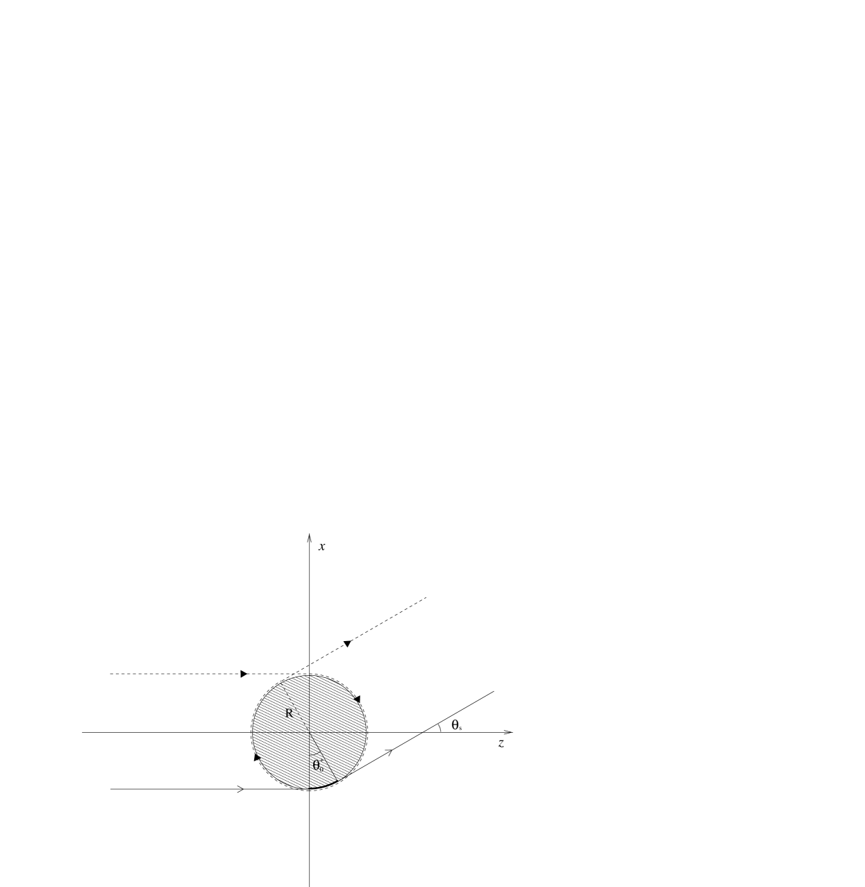
Figure 3: Diffractive scattering: geometry of the contribution of two grazing rays to the scattered amplitude. The ray below (solid line with open arrows) travels $\theta_{0}^{+}$ radians in the counterclockwise direction along the boundary of the obstacle, and leaves the obstacle in the direction of the scattering angle $\theta_{s}$ (see formula (72)). The ray above (solid and dashed lines with filled arrows) travels in the clockwise direction along the surface of the obstacle and crosses the axial caustic twice before emerging in the direction of the scattering angle $\theta_{s}$ (see formula (73)).

3.3 Surface Waves in Diffractive Scattering

In the scattering theory the far field diffracted by the obstacle must be related to the incoming field whose source is located at great distance from the obstacle. Then, we have to consider the limit obtained when the source point $p_{0}$ is pushed to $-\infty$ and the observer to $+\infty$. Let us introduce an orthogonal system of axes $(x,y,z)$ in ${\mathord{\mathbb{R}}}^{3}$ whose origin coincides with the center of the sphere, and such that the $z$-axis, chosen parallel to the incoming beam of rays, is positively oriented in the direction of the outgoing rays (see Fig. 3). Let us introduce, in addition, the coordinates on the sphere: ${\bf r}_{0}$ is the radial vector, $\phi_{0}$ is the azimuthal angle, $\theta_{0}$ is the angle measured along the meridian circle from the point of incidence of the ray on the sphere. Finally, let $\tau$ be a parameter running along the ray; in particular we have (on the sphere): $\tau=R\theta_{0}$ ($R$ being the radius of the sphere). Now, consider the rays that leave the surface of the sphere after diffraction. In view of the fact that the interior of the space, outside the obstacle, can be regarded as a Riemannian euclidean space without boundary, eqs. (22, 23) hold true, and, in this case, read

$$\displaystyle\frac{d{\bf r}}{d\tau} = {\bf p},$$ (64)

$$\displaystyle\frac{d{\bf p}}{d\tau} = 0,$$ (65)

where ${\bf r}=(x,y,z)$, and ${\bf p}=\nabla\Phi$ ($\Phi=$ phase function). From eqs. (64, 65) we get:

$${\bf r}(\theta_{0},\phi_{0},\tau)={\bf r}_{0}(\phi_{0},\theta_{0})+\tau{\bf p}_{0}(\phi_{0},\theta_{0}),$$ (66)

where ${\bf p}_{0}$ is the unit vector tangent to the obstacle where the ray leaves the sphere.

Let us now focus our attention on the ray hitting the sphere at the point of coordinates $(-R,0,0)$, and then traveling in counterclockwise sense. The components of the radial vector are (see Fig. 3): ${\bf r}_{0}=(-R\cos\theta_{0}\cos\phi_{0},R\cos\theta_{0}\sin\phi_{0},R\sin\theta_{0})$, and ${\bf p}_{0}=(\sin\theta_{0}\,\cos\phi_{0},-\sin\theta_{0}\sin\phi_{0},\cos\theta_{0})$. Substituting these expressions in Eq. (66) we have:

$${\bf r}(\theta_{0},\phi_{0},\tau)=(-R\cos\theta_{0}\cos\phi_{0}+\tau\sin\theta_{0}\cos\phi_{0},R\cos\theta_{0}\sin\phi_{0}-\tau\sin\theta_{0}\sin\phi_{0},R\sin\theta_{0}+\tau\cos\theta_{0}).$$ (67)

Now, the domain where the Jacobian $J={\displaystyle\frac{\partial(x,y,z)}{\partial(\theta_{0},\phi_{0},\tau)}}=\tau(R\cos\theta_{0}-\tau\sin\theta_{0})$ vanishes is composed by:

1. the surface of the sphere, where $\tau=0$;

2. the semi-axis represented by $\tau=\bar{\tau}=R\,\cot\,\theta_{0}$.

We can rewrite the transport equation (19) in the following form [10]:

$$\frac{1}{J}\frac{d}{d\tau}(JA^{2})=0,$$ (68)

whose solution $A=C/\sqrt{J}$ indicates once again that the amplitude becomes infinite for $J=0$, i.e. on the caustic. In order to treat the scattering problem we must perform the limit for $r\rightarrow+\infty$ ($r=|{\bf r}|$). Since $\tau=\sqrt{r^{2}-R^{2}}$, then as $r\rightarrow\infty$, $\tau$ tends to $r$, and from the expression of the Jacobian, we obtain: $\sqrt{J}\mathrel{\mathop{\displaystyle\longrightarrow}\limits_{r\rightarrow+\infty}}i\,r\,\sqrt{\sin\theta_{0}}$.

Now, let us revert to formula (53) in order to evaluate the contribution due to the diffracted ray. Recalling the asymptotic behaviour of Ai  and $\mbox{Ai\,}^{\prime}$, and by noting that in the present geometry $\Theta_{0}=R\theta_{0}+\tau$, and that the length of the arc described by the diffracted ray on the sphere is $l=R\theta_{0}$, we obtain, for $k\rightarrow+\infty$ and for large values of $r$ (see formula (63) and Ref. [28]):

$$u_{i}(k,\theta_{0},r)\mathrel{\mathop{\longrightarrow}\limits_{\mathrel{\mathop{\scriptstyle k\rightarrow\infty}\limits_{\scriptstyle r\rightarrow\infty}}}}C_{i}^{(d)}(k)\,\frac{e^{ikr}}{r}\,\frac{e^{-\beta_{i}R\,\theta_{0}}e^{ikR\,\theta_{0}}}{i\sqrt{\sin\theta_{0}}},$$ (69)

$(0<\theta_{0}<\pi)$, where $\beta_{i}$ is the exponent of the $i$-th damping factor $\alpha_{i}$ obtained in Section 3.2. For what concerns the diffraction coefficients $C_{i}^{(d)}(k)$, they have been derived by Lewis, Bleinstein and Ludwig [28] by assuming that the amplitude of the diffracted wave is proportional to the amplitude of the incident wave. In the present geometry these coefficients read

$$C_{i}^{(d)}(k)=\mbox{const.\,}\frac{(kR)^{1/3}}{[\mbox{Ai\,}^{\prime}(q_{i})]^{2}},$$ (70)

($q_{i}$ being the zeros of the Airy function), and coincide with the expression derived by Levy-Keller (see Table I of Ref. [4]). Since the roots of the Airy function are infinite, we have, correspondingly, a countably infinite set of modes $u_{i}$. For the moment we focus our attention on the damping factor $\alpha_{0}$, whose exponent $\beta_{0}$ is the smallest one, and, accordingly, on the mode $u_{0}$ that, for large values of $k$ and $r$, reads

$$u_{0}(k,\theta_{0},r)\mathrel{\mathop{\longrightarrow}\limits_{\mathrel{\mathop{\scriptstyle k\rightarrow\infty}\limits_{\scriptstyle r\rightarrow\infty}}}}-i\,C_{0}^{(d)}(k)\,\frac{e^{ikr}}{r}\frac{e^{i\lambda_{0}\theta_{0}}}{\sqrt{\sin\theta_{0}}},$$ (71)

$(0<\theta_{0}<\pi,\,\lambda_{0}=R\,(k+i\beta_{0}))$.

In order to evaluate the contribution to the scattering amplitude, the scattering angle $\theta_{s}$ must be related to the surface angle $\theta_{0}$. To distinguish between the contribution of the counterclockwise rays and that of the clockwise ones, we add the superscript ’$+$’ to all what refers to the counterclockwise rays, and the superscript ’$-$’ to all the symbols referring to the clockwise oriented rays. With this convention, and observing that $\theta_{s}=\theta_{0}^{+}$ (see Fig. 3), the contribution to the scattering amplitude $f^{+}_{(0,0)}$ of the counterclockwise grazing ray that has not completed one tour around the obstacle can be written as

$$f^{+}_{(0,0)}(k,\theta_{s})=C_{0}^{(d)}(k)\,\frac{e^{i\lambda_{0}\theta_{s}}e^{-i\pi/2}}{\sqrt{\sin\theta_{s}}},~{}~{}~{}~{}~{}(0<\theta_{s}<\pi).$$ (72)

Notice that in formula (72) the factor $\exp\{-i\pi/2\}$ corresponds to the Maslov phase-shift due to the fact that the ray crosses the axial caustic once (see Fig. 3).

Analogously, the contribution to the scattering amplitude $f^{-}_{(0,0)}$ of a diffracted ray which travels around the sphere, in clockwise sense, without completing one tour around the obstacle (see Fig. 3) can be evaluated. To this purpose, it is convenient to consider the asymptotic limit of $|J|^{1/2}$, which is given by $r\,|\sin\theta_{0}^{-}|^{1/2}$. Since the scattering angle $\theta_{s}$ is related to the surface angle $\theta_{0}^{-}$ as follows: $\theta_{0}^{-}=2\pi-\theta_{s}$, and by noting that this (clockwise oriented) grazing ray crosses the axial caustic (i.e. the $z$-axis) two times (see Fig. 3), we have:

$$f^{-}_{(0,0)}(k,\theta_{s})=(-1)\,C_{0}^{(d)}(k)\,\frac{e^{i\lambda_{0}(2\pi-\theta_{s})}}{\sqrt{\sin\theta_{s}}},~{}~{}~{}~{}~{}(0<\theta_{s}<\pi),$$ (73)

where the factor $(-1)$ is precisely given by the product of two Maslov factors (see Section 3.1).
Adding $f^{+}_{(0,0)}$ to $f^{-}_{(0,0)}$, we obtain the scattering amplitude $f_{(0,0)}(k,\theta_{s})$ due to the rays not completing one tour around the obstacle:

$$~{}~{}f_{(0,0)}(k,\theta_{s})=f^{+}_{(0,0)}+f^{-}_{(0,0)}=-i\,C_{0}^{(d)}(k)\,\frac{e^{i\lambda_{0}\theta_{s}}-ie^{i\lambda_{0}(2\pi-\theta_{s})}}{\sqrt{\sin\theta_{s}}},~{}~{}~{}~{}~{}(0<\theta_{s}<\pi).$$ (74)

Now, we are ready to take into account the contribution of all those rays which are orbiting around the sphere several times. Let us consider the rays describing $n$ ($n\in{\mathord{\mathbb{N}}}$) tours around the obstacle. Since the surface angles $\theta_{0,n}^{\pm}$ are related to the scattering angle $\theta_{s}$ as $\theta_{0,n}^{+}=\theta_{s}+2\pi n$, $\theta_{0,n}^{-}=2\pi-\theta_{s}+2\pi n$ $(n=0,1,2,\ldots)$, we have for $0<\theta_{s}<\pi$:

$$f_{0}(k,\theta_{s})=-i\,C_{0}^{(d)}(k)\sum_{n=0}^{\infty}(-1)^{n}\,e^{i2\pi n\lambda_{0}}\,\frac{e^{i\lambda_{0}\theta_{s}}-ie^{i\lambda_{0}(2\pi-\theta_{s})}}{\sqrt{\sin\theta_{s}}}.$$ (75)

The factor $(-1)$, at each $n$, is due to the product of two Maslov phase factors, corresponding to the fact that both the counterclockwise and the clockwise rays cross the $z$-axis (i.e. the axial caustic) twice for each tour (see Section 3.1).

Now, we exploit the following expansion:

$$\frac{1}{2\cos\pi\lambda_{0}}=e^{i\pi\lambda_{0}}\sum_{n=0}^{\infty}(-1)^{n}e^{i2\pi n\lambda_{0}},~{}~{}~{}~{}~{}(\mbox{Im}\,\lambda_{0}>0).$$ (76)

By the use of formula (76), the amplitude (75) can be rewritten as

$$~{}~{}f_{0}(k,\theta_{s})=-C_{0}^{(d)}(k)\,e^{i\pi/4}\,\frac{e^{-i\,\{\lambda_{0}(\pi-\theta_{s})-\pi/4\}}+e^{\,i\,\{\lambda_{0}(\pi-\theta_{s})-\pi/4\}}}{(2\cos\pi\lambda_{0})\>\sqrt{\sin\theta_{s}}},~{}~{}~{}~{}~{}(0<\theta_{s}<\pi).$$ (77)

The r.h.s. of formula (77) contains the asymptotic behaviour, for $|\lambda_{0}|\rightarrow\infty$ and $|\lambda_{0}|(\pi-\theta_{s})>>1$, of the Legendre function $P_{\lambda_{0}-\frac{1}{2}}(-\cos\theta_{s})$ times $\sqrt{2\pi\lambda_{0}}$ [34]. Then, writing $P_{\lambda_{0}-\frac{1}{2}}(-\cos\theta_{s})$ in place of its asymptotic behaviour, we have for $|\lambda_{0}|\rightarrow\infty$ $(0<\theta_{s}\leq\pi)$:

$$f_{0}(k,\theta_{s})\simeq-C_{0}^{(d)}(k)e^{i\pi/4}\,\frac{\sqrt{2\pi\lambda_{0}}\,P_{\lambda_{0}-\frac{1}{2}}(-\cos\theta_{s})}{2\cos\pi\lambda_{0}},$$ (78)

that, by putting $\mu_{0}=\lambda_{0}-1/2$, becomes

$$f_{0}(k,\theta_{s})\simeq C_{0}^{(d)}(k)\,e^{i\pi/4}\,\frac{\sqrt{\pi}}{2}\,\sqrt{(2\mu_{0}+1)}\,\frac{P_{\mu_{0}}(-\cos\theta_{s})}{\sin\pi\mu_{0}}.$$ (79)

Now, if we consider the countable infinity of damping factors $\alpha_{i}$ (see Section 3.2), we obtain an infinite set of creeping waves, whose angular distribution is described by the Legendre functions $P_{\mu_{i}}(-\cos\theta_{s})$, where $\mu_{i}=\lambda_{i}-1/2,~{}\lambda_{i}=R(k+i\beta_{i})$.

Let us recall that the simplest approach to diffraction scattering by a sphere is the expansion of the scattering amplitude in terms of spherical functions. But, when the radius of the sphere is large compared to the wavelength, these series converge so slowly that they become practically useless (see Refs. [18, 19]). A typical example of this difficulty is given by the diffraction of the radio waves around the earth. In order to remedy this drawback, Watson [19] proposed a resummation of the series that makes use of the analytic continuation from integer values $l$ of the angular momentum to complex $\lambda$-values (or $\mu$-values in our case). In this method the sum over integral $l$ is substituted by a sum over an infinite set of poles corresponding to the infinite set of creeping waves, whose angular distribution is described by the Legendre functions $P_{\mu_{i}}(-\cos\theta_{s})$. Let us note that at $\theta_{s}=0$, $P_{\mu_{i}}(-\cos\theta_{s})$ presents a logarithmic singularity [18], and, consequently, approximation (79) fails. Furthermore, at small angles the surface waves describe a very small arc of circumference, and the damping factors $\alpha_{i}$ are close to 1; therefore, we are obliged to take into account the contribution of the whole set of creeping waves. On the other hand, at $\theta_{s}=\pi$, $P_{\mu_{i}}(-\cos\theta_{s})=1$ and, furthermore, at large angles, the main contribution comes from that creeping wave whose damping factor $\alpha_{0}=\exp(-\beta_{0}l)$ has the smallest exponent $\beta_{0}$. Therefore, in the backward angular region the surface wave contribution is dominant, and the scattering amplitude can be approximately represented as follows:

$$f(k,\theta_{s})\simeq f_{0}(k,\theta_{s})={\cal G}_{0}(k)\,P_{\mu_{0}}(-\cos\theta_{s}),~{}~{}~{}~{}~{}(\theta_{s}>0),$$ (80)

where ${\cal G}_{0}(k)=C_{0}^{(d)}(k)\,e^{i\frac{\pi}{4}}\,(\frac{\sqrt{\pi}}{2})\,(2\mu_{0}+1)^{1/2}/\sin\pi\mu_{0}$.

4 Conclusions

Let us conclude with a brief remark on the difference between complex and diffracted rays. Complex rays are well known in optics in total reflection, where they describe the exponentially damped penetration into the rarer medium associated with surface waves traveling along the boundary. Then, it is very tempting to describe diffraction in terms of complex rays. Conversely, in the theory of diffraction which we present in this paper, we do not make any use of complex rays, but rather we introduce the diffracted rays, that are real. The first difficulty which emerges in this approach is the proof of the existence of these diffracted rays. This problem is solved by showing the non-uniqueness of the Cauchy problem for the geodesics in a Riemannian manifold with boundary. Then, since the border of the obstacle is the envelope of the diffracted rays, and the standard method of the stationary phase cannot be used, we are forced to apply a modified stationary phase method due to Chester, Friedman and Ursell [12]. By using this method we derive an infinite set of damping factors associated with the waves creeping around the obstacle. These damping factors have again a geometrical nature, since they depend on the curvature of the obstacle. In conclusion, it worth remarking that if we pass from optics to mechanics, and we consider particle trajectories instead of light rays, the splitting of geodesics at the boundary introduces a probabilistic aspect reflecting the fact that, at any point of the boundary, the particle can continue to orbit around the obstacle or can leave the obstacle itself. Therefore, using the damping factors is a way to connect probability, proper of semi–classical mechanics, to geometry: i.e. the curvature of the obstacle.

Acknowledgments

It is a pleasure to thank our friend Prof. M. Grandis for several helpful discussions.

References

- [1]
- [2] J. B. Keller, Proc. Symposia Appl. Math. 8 (1958) 27.
- [3] J. B. Keller, J. Opt. Soc. Am. 52 (1962) 116.
- [4] B. Levy and J. B. Keller, Commun. Pure Appl. Math. 12 (1959) 159.
- [5] D. Bouche, F. Molinet and R. Mittra, Asymptotic Methods in Electromagnetics, Springer–Verlag, Berlin, 1997.
- [6] S. B. Alexander, I. D. Berg and R. L. Bishop, Lecture Notes in Math. 1209 (1986) 1.
- [7] S. B. Alexander, I. D. Berg and R. L. Bishop, Illinois J. Math. 31 (1987) 167.
- [8] M. V. Berry and C. Upstill, Prog. Optics 18 (1980) 257.
- [9] J. Milnor, Morse Theory, Princeton University Press, Princeton, NJ, 1963.
- [10] V. P. Maslov and M. V. Fedoryuk, Semi-Classical Approximation in Quantum Mechanics, D. Reidel Publishing, Dordrecht, 1981.
- [11] A. S. Mishchenko, V. E. Shatalov and B. Y. Sternin, Lagrangian Manifolds and the Maslov Operator, Springer-Verlag, Berlin, 1980.
- [12] C. Chester, B. Friedman and F. Ursell, Proc. Cambridge Phil. Soc. 54 (1957) 599.
- [13] Y. A. Kravtsov, Radiofizika 7 (1964) 664.
- [14] D. Ludwig, Commun. Pure Appl. Math. 19 (1966) 215.
- [15] W. G. Neubauer, “Observation of Acoustic Radiation from Plane and Curved Surfaces”, pp. 61–126 in Physical Acoustics 10, W. P. Mason and R. N. Thurston, eds., Academic Press, New York, 1973.
- [16] R. Fioravanti and G. A. Viano, Phys. Rev. C 55 (1997) 2593.
- [17] A. Besse, Manifolds all of whose Geodesics are Closed, Springer–Verlag, Berlin, 1978.
- [18] A. Sommerfeld, Partial Differential Equations in Physics, Academic Press, New York, 1964.
- [19] G. N. Watson, Proc. Roy. Soc. London 95 (1918) 83.
- [20] H. M. Nussenzveig, Diffraction Effects in Semiclassical Scattering, Cambridge University Press, Cambridge, 1992, (see also the papers quoted therein).
- [21] H. Goldstein, Classical Mechanics, Addison-Wesley, Reading, 1959.
- [22] C. Plaut, Compositio Mathematica 81 (1992) 337.
- [23] S. Kobayashi, “On Conjugate and Cut Loci”, pp. 96–122 in Studies in Global Geometry and Analysis, S. S. Chern, ed., MAA Studies in Math. 4, 1967.
- [24] S. B. Alexander, Springer Lecture Notes 838 (1981) 12.
- [25] J. B. Delos, Adv. Chem. Phys. 65 (1986) 161.
- [26] V. P. Maslov, Operational Methods, Mir Publishers, Moscow, 1973.
- [27] V. Guillemin and S. Sternberg, Geometric Asymptotics, in Mathematical Surveys 14, American Mathematical Society, Providence, 1977.
- [28] R. M. Lewis, N. Bleinstein and D. Ludwig, Commun. Pure Appl. Math. 20 (1967) 295.
- [29] M. V. Berry and C. J. Howls, Proc. R. Soc. Lond. A 443 (1993) 107.
- [30] M. V. Berry and C. J. Howls, Proc. R. Soc. Lond. A 444 (1994) 201.
- [31] J. N. L. Connor, P. R. Curtis and R. A. W. Young, “Uniform Asymptotics of Oscillating Integrals: Applications in Chemical Physics”, pp. 24–38 in Wave Asymptotics, P. A. Martin and G. R. Wickham, eds., Cambridge University Press, Cambridge, 1992, (see also the papers quoted therein).
- [32] M. V. Berry, Adv. Phys. 25 (1976) 1.
- [33] J. N. L. Connor, Molecular Phys. 31 (1976) 33.
- [34] A. Erdelyi, W. Magnus, F. Oberhettinger and F. G. Tricomi, Higher Trascendental Functions, Vol. 1, McGraw-Hill, New York, 1953.