Random Distance Distribution for Spherical Objects: General Theory and Applications to $n$-Dimensional Physics

Abstract

A formalism is presented for analytically obtaining the probability density function, $P_{n}(s)$, for the random distance $s$ between two random points in an $n$-dimensional spherical object of radius $R$. Our formalism allows $P_{n}(s)$ to be calculated for a spherical $n$-ball having an arbitrary volume density, and reproduces the well-known results for the case of uniform density. The results find applications in stochastic geometry, computational science, molecular biological systems, statistical physics, astrophysics, condensed matter physics, nuclear physics, and elementary particle physics. As one application of these results, we propose a new statistical method obtained from our formalism to study random number generators in $n$-dimensions used in Monte Carlo simulations.

I Introduction

In two recent papers  D. Schleef, M. Parry, S. J. Tu, B. Woodahl, and E. Fischbach (1999); Parry and Fischbach (2000), geometric probability techniques were developed to calculate the functions $P_{3}\left(s\right)$ which describe the probability density of finding a random distance $s$ separating two random points distributed in a uniform sphere and in a uniform ellipsoid. As discussed in Refs. D. Schleef, M. Parry, S. J. Tu, B. Woodahl, and E. Fischbach (1999); Parry and Fischbach (2000); Deltheil (1919); Hammersley (1950); Lord (1954); Kendall and Moran (1963); Santaló (1976); Overhauser ; Fischbach (1996); E. Fischbach, D. E. Krause, C. Talmadge, and D. Tadić (1995); Tu (2001); Fedotov (1998); Jansons (1991); Mecke (1998); Miles (1980), these results are of interest as tools in mathematical physics, and have numerous applications in other fields as well. Specifically, it was demonstrated in Refs. D. Schleef, M. Parry, S. J. Tu, B. Woodahl, and E. Fischbach (1999); Parry and Fischbach (2000); Fischbach (1996); E. Fischbach, D. E. Krause, C. Talmadge, and D. Tadić (1995); Tu (2001) that knowing the random distance distribution in a spherical object greatly facilitates the calculation of self-energies for spherical matter distributions arising from electromagnetic, gravitational, or weak interactions.

As an example we calculate the total electrostatic energy $W_{3}$ of a collection of $Z$ charges uniformly distributed within the same spherical volume of radius $R$. For illustrative purposes, we assume that $Z$ is a large number. For each pair of charges the potential energy due to the Coulomb interaction in Gaussian units is

$$V_{3}=\frac{e^{2}}{r_{12}}=\frac{e^{2}}{\left|\vec{r}_{2}-\vec{r}_{1}\right|},$$ (1)

where $e$ is the elementary charge, $\vec{r}_{1}$ ($\vec{r}_{2}$) is the coordinate of the first (second) charge. The total Coulomb energy $W_{3}$ can then be expressed as

$$W_{3} = \frac{1}{2}\times\rho^{2}\int r_{1}^{2}\,dr_{1}\int\sin\theta_{1}\,d\theta_{1}\int\,d\phi_{1}\int r_{2}^{2}\,dr_{2}\int\sin\theta_{2}\,d\theta_{2}\int\frac{1}{r_{12}}\,d\phi_{2}$$ (2)

$$= \frac{Z^{2}}{2}\times\frac{6}{5}\frac{e^{2}}{R},$$

where $\rho=3Ze/4\pi R^{3}$ Jackson (1999). We note that Eq. (2) requires evaluating a six-dimensional integral, and using the additional theorem for spherical harmonics Arfken and Weber (1995),

$$P_{l}\left(\cos\gamma\right)=\frac{4\pi}{2l+1}\sum_{m=-l}^{l}\left(-1\right)^{m}Y^{m}_{l}\left(\theta_{1},\phi_{1}\right)Y_{l}^{-m}\left(\theta_{2},\phi_{2}\right).$$ (3)

Alternatively we can use the probability density function $P_{3}\left(s\right)$ giving the random distance distribution for a sphere with a uniform density to calculate $W_{3}$. For a collection of $Z$ charges there are $Z\left(Z-1\right)/2$ such pairs, and hence the total Coulomb energy $W_{3}$ is:

$$W_{3}=\frac{Z\left(Z-1\right)}{2}\times\int_{0}^{2R}P_{3}\left(s\right)\,\frac{e^{2}}{s}\,ds=\frac{Z\left(Z-1\right)}{2}\times\frac{6}{5}\frac{e^{2}}{R}\cong\frac{Z^{2}}{2}\times\frac{6}{5}\frac{e^{2}}{R},$$ (4)

where Deltheil (1919)

$$P_{3}\left(s\right)=3\frac{s^{2}}{R^{3}}-\frac{9}{4}\frac{s^{3}}{R^{4}}+\frac{3}{16}\frac{s^{5}}{R^{6}}.$$ (5)

We note that by using geometric probability techniques we can simplify the expression for $W_{3}$ from a six-dimensional non-trivial integral (Eq. (2)) to a one-dimensional elementary integral (Eq. (4)). Generalizing to $n$-dimensions, a calculation of the electrostatic energy $W_{n}$ for a collection of $Z$ charges uniformly distributed within the same $n$-dimensional spherical volume of radius $R$, can be greatly simplified by utilizing the $n$-dimensional random distance distribution. This reduces the complexity of calculating $W_{n}$ from a $2n$-dimensional intractable integral involving $n$-dimensional spherical harmonics, to a simple $1$-dimensional integral.

The probability density function $P_{n}(s)$ for the distribution of the random distance $s$ between two random points in a uniform spherical $n$-ball is well known. Hence the object of the present paper is to generalize the results of Refs. Kendall and Moran (1963); Santaló (1976); Overhauser to the case of an arbitrarily non-uniform density distribution by using a new method which we present below. Notice that the sample space $\mathbf{B}_{n}$ for the random points is a spherical $n$-ball of radius $R$ defined as

$$\mathbf{B}_{n}=\left\{\left(x_{1},x_{2},\cdots,x_{n}\right)\in\mathbf{R}^{n}:x_{1}^{2}+x_{2}^{2}+\cdots+x_{n}^{2}\leq R^{2}\right\},$$ (6)

where

$$\mathbf{R}^{n}=\left\{\bm{x}:\bm{x}=\left(x_{1},x_{2},\cdots,x_{n}\right)\right\}$$ (7)

represents $n$-dimensional Euclidean space.

To illustrate our formalism, we begin by deriving the probability density function (PDF) for a spherical $n$-ball with a uniform density distribution, and compare our results to those obtained earlier by other means Kendall and Moran (1963); Santaló (1976); Overhauser . We then extend this technique to a spherical $n$-ball with an arbitrary density distribution, and this leads to a general-purpose master formula for $P_{n}\left(s\right)$ given in Eq. (39). The outline of this paper is as follows. In Sec. II we present our formalism and illustrate it by rederiving the well-known results for a circle and for a sphere of uniform density. In Sec. III we extend this formalism to the case of non-uniform but spherically symmetric density. In Sec. IV we develop the formalism for the most general case of an arbitrary density distribution. In Sec. V we present some applications of our results. These include the $m$th moment $\left\langle s^{m}\right\rangle$ for a spherical space with a uniform and Gaussian density distribution, the evaluation of the self-energy arising from $\nu\bar{\nu}$-exchange interactions, the probability density functions for a sphere with multiple shells that arises in neutron star model Pines (1980); Shapiro and Teukolsky (1983), and finally a new proposed computational scheme for testing random number generators in $n$-dimensions.

II Uniform Density Distributions

In this section we illustrate our formalism by deriving the PDF for a circle of radius $R$ having a spatially uniform density characterized by a density function $\rho$, where $\rho$ is an arbitrary constant. For two points randomly sampled inside the circle located at $\vec{r}_{1}$ and $\vec{r}_{2}$ measured from the center, define a random vector $\vec{s}=\vec{r}_{2}-\vec{r}_{1}$ and a random distance $s=\left|\vec{s}\,\right|$, where $0\leq s\leq 2R$. To simplify the discussion, we translate the center of the circle to the origin so that the equation for the circle is $x^{2}+y^{2}=R^{2}$. It is sufficient to initially consider those vectors $\vec{s}\,$ which are aligned in the positive $\hat{x}$ direction, since rotational symmetry can eventually be used to extend our results to those vectors $\vec{s}\,$ with arbitrary orientations. We begin by identifying those pairs of points, $\vec{r}_{1}$ and $\vec{r}_{2}$, which satisfy $\vec{s}=s\hat{x}$. One set of random points for $\vec{r}_{1}$ is located in $A_{1}$ and the other set of random points for $\vec{r}_{2}$ is located in $A_{2}$ as shown in Fig. 1. We observe that $A_{2}$ is the overlap area between the original circle $C_{1}$ and an identical circle $C_{2}$ whose center is shifted from $\left(0,0\right)$ to $\left(\left|\vec{s}\,\right|,0\right)$ as shown in Fig. 2. Since the areas of $A_{1}$ and $A_{2}$ are equal, it follows that the probability density of finding a given $s=\left|s\hat{x}\right|$ in a circle of uniform density is proportional to the area of $A_{2}$:

$$\int_{s-R}^{\frac{s}{2}}\,dx\int_{-\sqrt{R^{2}-\left(x-s\right)^{2}}}^{\sqrt{R^{2}-\left(x-s\right)^{2}}}\,dy+\int_{\frac{s}{2}}^{R}\,dx\int_{-\sqrt{R^{2}-x^{2}}}^{\sqrt{R^{2}-x^{2}}}\,dy.$$ (8)

Using rotational symmetry, this result can apply to any orientation of $\vec{s}$, where $0\leq\phi\leq 2\pi$, and hence the probability density $P_{2}\left(s\right)$ for a circle of uniform density can be factorized as

$$P_{2}\left(s\right)=2\pi s\times f\left(s\right),$$ (9)

where $f\left(s\right)$ is a function to be determined. If we impose the normalization requirement

$$\int_{0}^{2R}P_{2}(s)\,ds=1,$$ (10)

we then have

$$P_{2}(s) = \frac{2\pi s\int_{\frac{s}{2}}^{R}\,dx\int_{-\sqrt{R^{2}-x^{2}}}^{\sqrt{R^{2}-x^{2}}}\,dy}{\int_{0}^{2R}\left(2\pi s\int_{\frac{s}{2}}^{R}\,dx\int_{-\sqrt{R^{2}-x^{2}}}^{\sqrt{R^{2}-x^{2}}}\,dy\right)ds}$$ (11)

$$= \frac{2s}{R^{2}}-\frac{s^{2}}{\pi R^{4}}\sqrt{4R^{2}-s^{2}}-\frac{4s}{\pi R^{2}}\sin^{-1}\left(s/2R\right).$$ (12)

Equation (12) is identical to the results obtained in Refs. Kendall and Moran (1963); Santaló (1976) by other means.

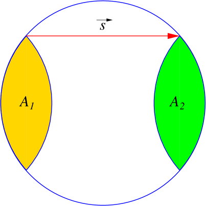
Figure 1: Locus of points in a circle separated by a vector $\vec{s}=s\hat{x}$. For each random point $\vec{r}_{1}$ in $A_{1}$. there is a unique random point $\vec{r}_{2}$ in $A_{2}$ such that $\vec{s}=\vec{r}_{2}-\vec{r}_{1}$.

The conclusion that emerges from this formalism is that the probability density of finding two random points separated by a random vector $\vec{s}\,$ in a circle of uniform density can be derived by simply calculating the overlap region of that circle with an identical circle obtained by shifting the center from the origin to $\vec{s}$. In the following discussion, we show that this result generalizes to higher dimensions, and provides a simple way of calculating $P_{n}(s)$ for $n\geq 3$.

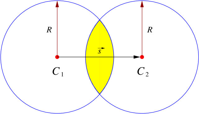
Figure 2: The probability density that two random points are separated by a random distance $\left|s\hat{x}\right|$ in a circle of radius $R$ is proportional to the shaded area given by the overlap of $C_{1}$ and $C_{2}$, where $C_{1}$ is $x^{2}+y^{2}=R^{2}$ and $C_{2}$ is $\left(x-s\right)^{2}+y^{2}=R^{2}$.

The above formalism for a circle of uniform density can be extended to a sphere of uniform density. For a given $s$, we select the positive $\hat{z}$ direction and study the distribution of the random vectors $\vec{s}\,$ in this direction. It then follows that the probability density of finding $s\hat{z}$ is proportional to

$$\int_{s-R}^{\frac{s}{2}}\,dz\int_{-\sqrt{R^{2}-\left(z-s\right)^{2}}}^{\sqrt{R^{2}-\left(z-s\right)^{2}}}\,dx\int^{\sqrt{R^{2}-\left(z-s\right)^{2}-x^{2}}}_{-\sqrt{R^{2}-\left(z-s\right)^{2}-x^{2}}}\,dy+\int_{\frac{s}{2}}^{R}\,dz\int_{-\sqrt{R^{2}-z^{2}}}^{\sqrt{R^{2}-z^{2}}}\,dx\int^{\sqrt{R^{2}-z^{2}-x^{2}}}_{-\sqrt{R^{2}-z^{2}-x^{2}}}\,dy.$$ (13)

In a $3$-dimensional space, we note that the direction of the random vector $\vec{s}\,$ can have the following range: $0\leq\theta\leq\pi$ and $0\leq\phi\leq 2\pi$. Following the previous discussion, we thus arrive at the following expression for a sphere with a uniform density distribution:

$$P_{3}(s) = \frac{4\pi s^{2}\left(\int_{\frac{s}{2}}^{R}\,dz\int_{-\sqrt{R^{2}-z^{2}}}^{\sqrt{R^{2}-z^{2}}}\,dx\int^{\sqrt{R^{2}-z^{2}-x^{2}}}_{-\sqrt{R^{2}-z^{2}-x^{2}}}\,dy\right)}{\int_{0}^{2R}4\pi s^{2}\left(\int_{\frac{s}{2}}^{R}\,dz\int_{-\sqrt{R^{2}-z^{2}}}^{\sqrt{R^{2}-z^{2}}}\,dx\int^{\sqrt{R^{2}-z^{2}-x^{2}}}_{-\sqrt{R^{2}-z^{2}-x^{2}}}\,dy\right)ds}$$ (14)

$$= 3\frac{s^{2}}{R^{3}}-\frac{9}{4}\frac{s^{3}}{R^{4}}+\frac{3}{16}\frac{s^{5}}{R^{6}}.$$ (15)

The result in Eq. (15) agrees exactly with the expression obtained previously in Refs. Kendall and Moran (1963); Santaló (1976); Overhauser ; Deltheil (1919); Hammersley (1950); Lord (1954).

The present formalism can be readily generalized to express $P_{n}\left(s\right)$ for a sphere of uniform density in $n$-dimensions as

$$P_{n}(s)=\frac{s^{n-1}\int_{s/2}^{R}\,dx_{n}\int_{-\sqrt{R^{2}-x_{n}^{2}}}^{\sqrt{R^{2}-x_{n}^{2}}}\,dx_{1}\cdots\int_{-\sqrt{R^{2}-x_{n}^{2}-\cdots x_{n-2}^{2}}}^{\sqrt{R^{2}-x_{n}^{2}-\cdots x_{n-2}^{2}}}\,dx_{n-1}}{\int_{0}^{2R}\left(s^{n-1}\int_{s/2}^{R}\,dx_{n}\int_{-\sqrt{R^{2}-x_{n}^{2}}}^{\sqrt{R^{2}-x_{n}^{2}}}\,dx_{1}\cdots\int_{-\sqrt{R^{2}-x_{n}^{2}-\cdots x_{n-2}^{2}}}^{\sqrt{R^{2}-x_{n}^{2}-\cdots x_{n-2}^{2}}}\,dx_{n-1}\right)ds}.$$ (16)

We find that if $n$ is an even number,

$$P_{n}(s)=\frac{n\times s^{n-1}}{R^{n}}\left[\frac{2}{\pi}\cos^{-1}\left(s/2R\right)-\frac{s}{\pi}\sum_{k=1}^{\frac{n}{2}}\frac{(n-2k)!!}{(n-2k+1)!!}\left(R^{2}-s^{2}/4\right)^{\frac{n-2k+1}{2}}R^{2k-2-n}\right],$$ (17)

where $0!=0!!=1$. If $n$ is an odd number,

$$P_{n}(s)=\frac{n\times s^{n-1}}{R^{n}}\frac{n!!}{(n-1)!!}\sum_{k=0}^{\frac{n-1}{2}}\frac{(-1)^{k}}{2k+1}\frac{\left(\frac{n-1}{2}\right)!}{k!\left(\frac{n-1}{2}-k\right)!}\left[1-\left(s/2R\right)^{2k+1}\right].$$ (18)

The functional forms of Eq. (16) for $n=1$, $2$, $3$, and $4$ are shown in Fig. 3.

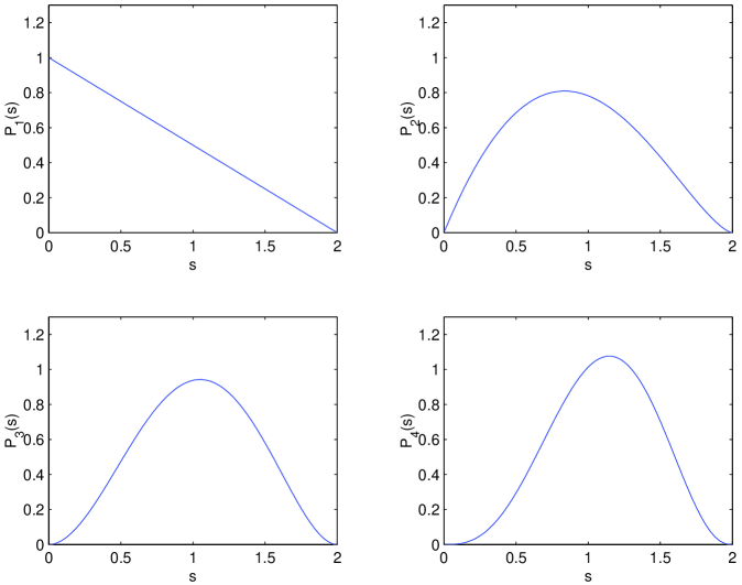
Figure 3: Plots of $P_{1}\left(s\right)$, $P_{2}\left(s\right)$, $P_{3}\left(s\right)$, and $P_{4}\left(s\right)$ for a uniform density distribution. Note that in all cases $\int_{0}^{2R}P_{n}(s)\,ds=1$.

The cumulative distribution function (CDF) Feller (1967); Gardiner (1985); van Kampen (1992) for $P_{n}(s)$ is given by

$$D_{n}(x) = \int_{0}^{x}P_{n}(s)\,ds$$ (19)

$$= \frac{x^{n}}{R^{n}}-\frac{B_{\alpha}\left(\frac{1}{2},\frac{n}{2}+\frac{1}{2}\right)}{B\left(\frac{1}{2},\frac{n}{2}+\frac{1}{2}\right)}\times\frac{x^{n}}{R^{n}}+2^{n}\times\frac{B_{\alpha}\left(\frac{n}{2}+\frac{1}{2},\frac{n}{2}+\frac{1}{2}\right)}{B\left(\frac{1}{2},\frac{n}{2}+\frac{1}{2}\right)},$$

where $0\leq x\leq 2R$, $\alpha=x^{2}/4R^{2}$, and $B_{\alpha}$ is the incomplete beta function.

We summarize three important representations for the probability density function $P_{n}\left(s\right)$ for a spherical $n$-ball of radius $R$ with a uniform density distribution as follows:

1. Integral representation:

   $$P_{n}(s)=\frac{s^{n-1}\int_{\frac{s}{2}}^{R}\left(R^{2}-x^{2}\right)^{\frac{n-1}{2}}\,dx}{\frac{1}{2n}B(\frac{n}{2}+\frac{1}{2},\frac{1}{2})R^{2n}}.$$ (20)

2. Generating function representation:

   $$P_{n}(s)=\frac{s^{n-1}\frac{1}{n!}\left(\frac{\partial}{\partial h}\right)^{n}_{h=0}\frac{1}{\sqrt{1-h^{2}}}\left[\sin^{-1}h-\sin^{-1}\left(\frac{2h-\sqrt{4-s^{2}}}{2-h\sqrt{4-s^{2}}}\right)\right]}{\frac{1}{2n}B(\frac{n}{2}+\frac{1}{2},\frac{1}{2})},$$ (21)

   where $\left|h\right|<1$ and $R=1$. We note that one can obtain a number of identities and recursion relations for $P_{n}\left(s\right)$ from the generating function representation in Eq. (21).

3. Hypergeometric function representation:

   $$P_{n}(s)=\frac{2n}{B\left(\frac{n}{2}+\frac{1}{2},\frac{1}{2}\right)}\times\left[\,{}_{2}F_{1}\left(a,b,c,\alpha\right)R-\frac{s}{2}\,\,_{2}F_{1}\left(a,b,c,\beta\right)\right]\times\frac{s^{n-1}}{R^{n+1}},$$ (22)

   where $a=1/2$, $b=1/2-n/2$, $c=3/2$, $\alpha=1$, $\beta=s^{2}/4R^{2}$, and $\,{}_{2}F_{1}\left(\cdots\right)$ is the hypergeometric function Arfken and Weber (1995). Notice that we can obtain the orthogonality relations for $P_{n}\left(s\right)$ from the hypergeometric function representation as shown in Eq. (22).

In Ref. Tu (2001) additional identities and recursion relations for $P_{n}\left(s\right)$ are discussed in greater detail.

III Spherically Symmetric Density Distributions

In this section we extend the previous results to the case of a circle with a variable (but spherically symmetric) density characterized by a density function $\rho\left(r\right)$. Following the derivation presented in the previous section, we note that for any random vector $\vec{s}=s\hat{x}$, if the second random point $\vec{r}_{2}$ carries the density information $\rho\left(x,y\right)$, then the first random point $\vec{r}_{1}$ should have the density information $\rho\left(x-s,y\right).$ It then follows $P_{2}(s)$ can be expressed as

$$P_{2}(s) = \frac{s\int_{\frac{s}{2}}^{R}\,dx\int_{-\sqrt{R^{2}-x^{2}}}^{\sqrt{R^{2}-x^{2}}}\rho\left(x-s,y\right)\times\rho\left(x,y\right)\,dy}{\int_{0}^{2R}\left(s\int_{\frac{s}{2}}^{R}\,dx\int_{-\sqrt{R^{2}-x^{2}}}^{\sqrt{R^{2}-x^{2}}}\rho\left(x-s,y\right)\times\rho\left(x,y\right)\,dy\right)ds}.$$ (23)

A general formula for $P_{n}\left(s\right)$ for an $n$-dimensional spherical ball of radius $R$ having a spherically symmetric density can be derived, and we find

$$P_{n}(s)=\frac{s^{n-1}\int_{\frac{s}{2}}^{R}\,dx_{n}\int_{-\sqrt{R^{2}-x_{n}^{2}}}^{\sqrt{R^{2}-x_{n}^{2}}}\,dx_{1}\cdots\int_{-\sqrt{R^{2}-x_{n}^{2}-x_{1}^{2}-\cdots x_{n-1}^{2}}}^{\sqrt{R^{2}-x_{n}^{2}-x_{1}^{2}-\cdots x_{n-1}^{2}}}\rho_{1}\times\rho_{2}\,dx_{n-1}}{\int_{0}^{2R}\left(s^{n-1}\int_{\frac{s}{2}}^{R}\,dx_{n}\int_{-\sqrt{R^{2}-x_{n}^{2}}}^{\sqrt{R^{2}-x_{n}^{2}}}\,dx_{1}\cdots\int_{-\sqrt{R^{2}-x_{n}^{2}-x_{1}^{2}-\cdots x_{n-1}^{2}}}^{\sqrt{R^{2}-x_{n}^{2}-x_{1}^{2}-\cdots x_{n-1}^{2}}}\rho_{1}\times\rho_{2}\,dx_{n-1}\right)ds},$$ (24)

where

$$\rho_{1} = \rho\left(x_{1},x_{2},\cdots,x_{n}-s\right),$$

$$\rho_{2} = \rho\left(x_{1},x_{2},\cdots,x_{n}\right).$$ (25)

Some analytical results for a sphere with various spherically symmetric density distributions can be found in Ref. Tu (2001).

As an application of Eq. (24) we consider the case of an $n$-dimensional spherical space of radius $R\rightarrow\infty$ with a Gaussian density given by

$$\rho_{n}(r)=\frac{N}{(2\pi)^{\frac{n}{2}}\sigma^{n}}e^{-\frac{1}{2}\frac{r^{2}}{\sigma^{2}}},$$ (26)

where

$$N=\lim_{R\rightarrow\infty}n\frac{\pi^{\frac{n}{2}}}{\Gamma\left(\frac{n}{2}+1\right)}\int_{0}^{R}\rho_{n}(r)r^{n-1}dr.$$ (27)

In Eq. (27) $r$ is measured from the center, and the integral is over all space. The PDF for an $n$-dimensional spherical Gaussian space can then be obtained as

$$P_{n}(s)=\frac{s^{n-1}e^{-\frac{s^{2}}{4\sigma^{2}}}}{2^{n-1}\Gamma\left(\frac{n}{2}\right)\sigma^{n}}.$$ (28)

Fig. 4 displays the functions in Eq. (28) for $n=3$, $4$, $5$, and $6$, where $\sigma=1$. Finally, we note that the maximum probability density, denoted by $s_{\mathrm{max}}$, occurs at

$$s_{\mathrm{max}}=\sqrt{2(n-1)}\,\sigma.$$ (29)

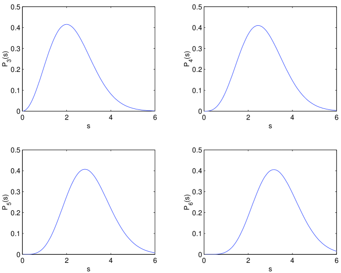
Figure 4: Plots of $P_{3}\left(s\right)$, $P_{4}\left(s\right)$, $P_{5}\left(s\right)$, and $P_{6}\left(s\right)$ for a Gaussian density distribution. Note that in all cases the functions are normalized such that $\int_{0}^{\infty}P_{n}(s)\,ds=1$.

IV Arbitrary Density Distributions

We consider in this section the probability density functions for a spherical $n$-ball having an arbitrary density characterized by a density function $\rho$. We begin with a circle and use the conventional notation for polar coordinates: $x=r\cos\phi$ and $y=r\sin\phi$. In a $2$-dimensional space, the random vector $\vec{s}\,$ can be characterized by an angle $\phi$ in the range $0\leq\phi\leq 2\pi$. Associate each random unit vector $\hat{s}\left(\phi\right)$ with a rotation operator $\mathscr{R}$ such that

$$\left|\hat{x}\right\rangle=\mathscr{R}\left|\hat{s}\left(\phi\right)\right\rangle.$$ (30)

To ensure that the product of $\rho\left(\vec{r}_{1}\right)$ and $\rho\left(\vec{r}_{2}\right)$ maintains the correct density information, we use a $2\times 2$ matrix

$$R_{2\times 2}(\phi)=\left[\begin{array}[]{cc}\cos\phi&-\sin\phi\\ \sin\phi&\cos\phi\end{array}\right]$$ (31)

to characterize this particular operator $\mathscr{R}$ such that

$$\rho(x,y)\longrightarrow\rho\left(\cos\phi\,x-\sin\phi\,y,\sin\phi\,x+\cos\phi\,y\right).$$ (32)

Notice that $R_{2\times 2}(\phi)$ is an orthogonal matrix which satisfies $R_{2\times 2}^{-1}(\phi)=R_{2\times 2}^{T}(\phi)$ and its determinant is $+1$, where $T$ denotes the transpose.

We can then express $P_{2}\left(s\right)$ for a circle with an arbitrary density distribution as

$$P_{2}(s)=\frac{s\int_{0}^{2\pi}\,d\phi\int_{s/2}^{R}\,dx\int_{-\sqrt{R^{2}-x^{2}}}^{\sqrt{R^{2}-x^{2}}}\rho\left(x^{\prime},y^{\prime}\right)\times\rho\left(x^{\prime\prime},y^{\prime\prime}\right)\,dy}{\int_{0}^{2R}\left(s\int_{0}^{2\pi}\,d\phi\int_{s/2}^{R}\,dx\int_{-\sqrt{R^{2}-x^{2}}}^{\sqrt{R^{2}-x^{2}}}\rho\left(x^{\prime},y^{\prime}\right)\times\rho\left(x^{\prime\prime},y^{\prime\prime}\right)\,dy\right)ds}$$ (33)

where

$$\rho\left(x^{\prime},y^{\prime}\right) = \rho\left(\cos\phi\,(x-s)-\sin\phi\,y,\,\sin\phi\,(x-s)+\cos\phi\,y\right),$$

$$\rho\left(x^{\prime\prime},y^{\prime\prime}\right) = \rho\left(\cos\phi\,x-\sin\phi\,y,\,\sin\phi\,x+\cos\phi\,y\right).$$

Figure 5 exhibits $P_{2}(s)$ when $R=1$, and illustrates the agreement between the Monte Carlo simulation and the analytical result.

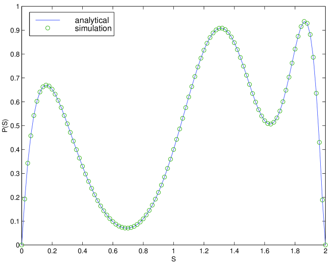
Figure 5: Plot of $P_{2}(s)$ as a function of $s$ for the case $R=1$ and $\rho\left(x,y\right)\propto x^{4}y^{4}$.

The preceding discussion can be generalized to the case of a spherical $n$-ball with an arbitrary density. Define the following hyperspherical coordinates Fleming (1977),

$$x_{1} = r\sin\theta_{n-2}\sin\theta_{n-3}\cdots\cdots\cdots\cdots\cdots\cdots\sin\theta_{2}\sin\theta_{1}\cos\phi,$$

$$x_{2} = r\sin\theta_{n-2}\sin\theta_{n-3}\cdots\cdots\cdots\cdots\cdots\cdots\sin\theta_{2}\sin\theta_{1}\sin\phi,$$

$$\vdots$$

$$x_{i} = r\sin\theta_{n-2}\sin\theta_{n-3}\cdots\cdots\sin\theta_{i-1}\cos\theta_{i-2},$$

$$\vdots$$

$$x_{n-1} = r\sin\theta_{n-2}\cos\theta_{n-3},$$

$$x_{n} = r\cos\theta_{n-2}.$$ (34)

where $\theta_{i}\in[0,\pi]$ and $\phi\in[0,2\pi]$. Associate each random unit vector $\hat{s}\left(\theta_{1},\cdots,\phi\right)$ with a rotation operator $\mathscr{R}$ such that

$$\left|\hat{x}_{n}\right\rangle=\mathscr{R}\left|\hat{s}\left(\theta_{1},\cdots,\phi\right)\right\rangle.$$ (35)

The $n\times n$ matrix representation for the rotation operator $\mathscr{R}$ in Eq. (35) can be expressed as

$$R_{n\times n}\left(\theta_{n-2},\cdots,\theta_{1},\phi\right)=R_{n\times n}(\phi)\times R_{n\times n}(\theta_{1})\times\cdots\times R_{n\times n}(\theta_{n-2}),$$ (36)

where $n\geq 3$. The various matrices on the right-hand side of Eq. (36) are defined as follows:

1. $R_{n\times n}(\phi)$: The matrix elements are $a_{11}=\cos\phi$, $a_{12}=-\sin\phi$, $a_{21}=\sin\phi$, $a_{22}=\cos\phi$, for $i\in[1,2]$ and $j\in[3,n]$ $a_{ij}=0$, for $i\in[3,n]$ and $i\in[1,2]$ $a_{ij}=0$, for $i\in[3,n]$ and $j\in[3,n]$ $a_{ij}=\delta_{ij}$.

2. $R_{n\times n}\left(\theta_{1}\right)$: The matrix elements are $a_{11}=\cos\theta_{1}$, $a_{12}=0$, $a_{13}=\sin\theta_{1}$, $a_{21}=0$, $a_{22}=1$, $a_{23}=0$, $a_{31}=-\sin\theta_{1}$, $a_{32}=0$, $a_{33}=\cos\theta_{1}$, for $i\in[1,3]$ and $j\in[4,n]$ $a_{ij}=0$, for $i\in[4,n]$ and $j\in[1,3]$ $a_{ij}=0$, for $i\in[4,n]$ and $j\in[4,n]$ $a_{ij}=\delta_{ij}$.

3. $R_{n\times n}\left(\theta_{k}\right)$ and $k\in[2,n-3]$: The matrix elements are $a_{k+1,k+1}=\cos\theta_{k}$, $a_{k+1,k+2}=\sin\theta_{k}$, $a_{k+2,k+1}=-\sin\theta_{k}$, $a_{k+2,k+2}=\cos\theta_{k}$, for $i\in[1,k]$ and $j\in[1,k]$ $a_{ij}=\delta_{ij}$, for $i\in[k+3,n]$ and $j\in[k+3,n]$ $a_{ij}=\delta_{ij}$, for $i\in[1,k]$ and $j\in[k+1,n]$ $a_{ij}=0$, for $i\in[k+1,n]$ and $j\in[1,k]$ $a_{ij}=0$, for $i\in[k+1,k+2]$ and $j\in[k+3,n]$ $a_{ij}=0$, for $i\in[k+3,n]$ and $j\in[k+1,k+2]$ $a_{ij}=0$.

4. $R_{n\times n}\left(\theta_{n-2}\right)$: The matrix elements are $a_{n-1,n-1}=\cos\theta_{n-2}$, $a_{n-1,n}=\sin\theta_{n-2}$, $a_{n,n-1}=-\sin\theta_{n-2}$, $a_{n,n}=\cos\theta_{n-2}$, for $i\in[1,n-2]$ and $j\in[1,n-2]$ $a_{ij}=\delta_{ij}$, for $i\in[1,n-2]$ and $j\in[n-1,n]$ $a_{ij}=0$, for $i\in[n-1,n]$ and $j\in[1,n-2]$ $a_{ij}=0$.

Notice that all the matrices in Eq. (36) are orthogonal and their determinants are $+1$. The matrix elements for $R_{n\times n}(\theta_{n-2},\cdots,\theta_{1},\phi)$ can be summarized as follows:

1. The matrix elements for the $1$st column are $a_{11}=\cos\theta_{1}\cos\phi$, $a_{21}=\cos\theta_{1}\sin\phi$, $a_{31}=-\sin\theta_{1}$, and for $i\in[4,n]$ $a_{i1}=0$.

2. The matrix elements for the $2$nd column are $a_{12}=-\sin\phi$, $a_{22}=\cos\phi$, and for $i\in[3,n]$ $a_{i2}=0$.

3. The matrix elements for the $j$th column where $j\in[3,n-1]$ are $a_{j+1,j}=-\sin\theta_{j-1}$, for $i\in[j+2,n]$ $a_{ij}=0$, and for $i\in[1,j]$ $a_{ij}=\cos\theta_{j-1}\times x_{i}$, where $x_{i}=\hat{r}\times\hat{x}_{i}$ and $x_{i}$ is the $i$th Cartesian coordinate component for a unit vector $\hat{r}$ in $j$-dimensions. For example:

   $$a_{14} = \cos\theta_{3}\sin\theta_{2}\sin\theta_{1}\cos\phi,$$

   $$a_{24} = \cos\theta_{3}\sin\theta_{2}\sin\theta_{1}\sin\phi,$$

   $$a_{34} = \cos\theta_{3}\sin\theta_{2}\cos\theta_{1},$$

   $$a_{44} = \cos\theta_{3}\cos\theta_{2}.$$

4. The matrix elements for the $n$th column are for $i\in[1,n]$ $a_{in}=x_{i}$, where $x_{i}=\hat{r}\times\hat{x}_{i}$ and $x_{i}$ is the $i$th Cartesian coordinate component for a unit vector $\hat{r}$ in $n$-dimensions.

Additionally, it is convenient to define the following transforms:

$$x_{i}^{\prime} = \sum_{j=1}^{n}a_{ij}\left(x_{j}-\delta_{jn}s\right),$$ (37)

$$x_{i}^{\prime\prime} = \sum_{j=1}^{n}a_{ij}x_{j},$$ (38)

where $a_{ij}$ are the matrix elements for $R_{n\times n}\left(\theta_{n-2},\cdots,\theta_{1},\phi\right)$ defined in Eq. (36). The master equation of $P_{n}(s)$ for a spherical $n$-ball with an arbitrary density characterized by a density function $\rho\left(\bm{x}\right)=\rho\left(x_{1},x_{2},\cdots,x_{n}\right)$ can then be formulated as

$$P_{n}(s)=\frac{s^{n-1}\times\mathbf{F}_{n}\left(x,\theta\right)}{\int_{0}^{2R}\left[s^{n-1}\times\mathbf{F}_{n}\left(x,\theta\right)\right]\,ds},$$ (39)

where

$$\mathbf{F}_{n}\left(x,\theta\right) = \int_{0}^{\pi}\sin^{n-2}\theta_{n-2}\,d\theta_{n-2}\int_{0}^{\pi}\sin^{n-3}\theta_{n-3}\,d\theta_{n-3}\cdots$$

$$\cdots\cdots\int_{0}^{\pi}\sin\theta_{1}\,d\theta_{1}\int_{0}^{2\pi}\,d\phi\int_{s/2}^{R}\,dx_{n}\int_{-\sqrt{R^{2}-x_{n}^{2}}}^{\sqrt{R^{2}-x_{n}^{2}}}\,dx_{1}\cdots$$

$$\cdots\cdots\cdots\int^{\sqrt{R^{2}-x_{n}^{2}-\cdots x_{n-2}^{2}}}_{-\sqrt{R^{2}-x_{n}^{2}-\cdots x_{n-2}^{2}}}\,\rho\left(\bm{x}^{\prime}\right)\times\rho\left(\bm{x}^{\prime\prime}\right)\,dx_{n-1},$$

and

$$\rho\left(\bm{x}^{\prime}\right) = \rho\left(x_{1}^{\prime},x_{2}^{\prime},\cdots,x_{n}^{\prime}\right),$$

$$\rho\left(\bm{x}^{\prime\prime}\right) = \rho\left(x^{\prime\prime}_{1},x^{\prime\prime}_{2},\cdots,x^{\prime\prime}_{n}\right).$$

The probability density function for the random distance distribution including Euclidean distance and geodesic distance for an $n$-dimensional sphere (i.e. the boundary of a spherical $n$-ball) with an arbitrary surface density distribution will be discussed in Ref. Tu (a).

V Applications

V.1 $m$th Moment of the Distance

In some applications the $m$th moment of the distance, rather than the distance itself, is of interest. As an example, for a collection of nucleons interacting via simple harmonic oscillator potentials, $\left\langle s^{2}\right\rangle$ may be of interest rather than $\left\langle s\right\rangle$ itself. We then calculate the $m$th moment $\left\langle s^{m}\right\rangle$ for the case of a spherical $n$-ball of uniform density, where

$$\left\langle s^{m}\right\rangle=\int_{0}^{2R}s^{m}P_{n}(s)\,ds.$$ (40)

Using Eq. (20), the $m$th moment $\left\langle s^{m}\right\rangle$ has the general form

$$\left\langle s^{m}\right\rangle=2^{n+m}\left(\frac{n}{n+m}\right)\frac{B\left(\frac{n}{2}+\frac{1}{2},\frac{n}{2}+\frac{1}{2}+\frac{m}{2}\right)}{B\left(\frac{n}{2}+\frac{1}{2},\frac{1}{2}\right)}R^{m},$$ (41)

where $B\left(p,q\right)$ is the beta function, and $m\geq-\left(n-1\right)$.

Additionally, $\left\langle s^{m}\right\rangle$ can be evaluated for a spherical space having a Gaussian density distribution where $\rho\propto e^{-r^{2}/2\sigma^{2}}$. From Eq. (28) we find,

$$\left\langle s^{m}\right\rangle=\lim_{R\rightarrow\infty}\int_{0}^{2R}s^{m}P_{n}(s)ds=(2\sigma)^{m}\frac{\Gamma\left(\frac{n+m}{2}\right)}{\Gamma\left(\frac{n}{2}\right)}.$$ (42)

In some applications (such as in nuclear physics) involving low-energy interactions among nucleons the lower limit (zero) should be replaced by the hard-core radius $r_{c}\cong 0.5\times 10^{-13}$ cm Bohr and Mottelson (1969). In such cases the expressions for $P_{n}(s)$ and $\left\langle s^{m}\right\rangle$ can be expressed as follows:

$$P_{n}(s)=\frac{s^{n-1}\int_{\frac{s}{2}}^{R}\left(R^{2}-x^{2}\right)^{\frac{n-1}{2}}\,dx}{C(2R,0,n)-C(r_{c},0,n)}$$ (43)

and

$$\left\langle s^{m}\right\rangle=\int_{r_{c}}^{2R}s^{m}P_{n}(s)\,ds=\frac{H(R,r_{c},m,n)}{H(R,r_{c},0,n)},$$ (44)

where

$$C\left(a,m,n\right)=\int_{0}^{a}s^{m+n-1}\,ds\int_{s/2}^{R}\left(R^{2}-x^{2}\right)^{\left(n-1\right)/2}\,dx,$$

and

$$H\left(R,r_{c},m,n\right) = \frac{(2R)^{n+m}}{n+m}\left[B\left(\frac{n}{2}+\frac{1}{2},\frac{n}{2}+\frac{1}{2}+\frac{m}{2}\right)-B_{x}\left(\frac{n}{2}+\frac{1}{2},\frac{n}{2}+\frac{1}{2}+\frac{m}{2}\right)\right]$$ (45)

$$-\frac{r_{c}^{n+m}}{n+m}\left[B\left(\frac{1}{2},\frac{n}{2}+\frac{1}{2}\right)-B_{x}\left(\frac{1}{2},\frac{n}{2}+\frac{1}{2}\right)\right],$$

with $x=r_{c}^{2}/4R^{2}$, and $m$ an integer. We note that Eqs. (43) and (44) are the first known analytical results for $P_{n}(s)$ and $\left\langle s^{m}\right\rangle$ to incorporate the hard-core radius $r_{c}$.

V.2 Neutrino-Pair Exchange Interactions

A second example of interest is the $\nu\bar{\nu}$-exchange (neutrino-pair exchange) contribution to the self energy of a nucleus or a neutron star. For two point masses the $2$-body potential energy is given by Fischbach (1996); Feinberg and Sucher (1968); G. Feinberg, J. Sucher, and C. K. Au (1989); Hsu and Sikivie (1994); Woodahl and Fischbach (2000a, b, 2001)

$$V_{\nu\bar{\nu}}\left(\left|\vec{r}_{i}-\vec{r}_{j}\right|\right)=\frac{G_{F}^{2}\,a_{i}a_{j}}{4\pi^{3}\left|\vec{r}_{i}-\vec{r}_{j}\right|^{5}},$$ (46)

where $a_{i}$ and $a_{j}$ are coupling constants which characterize the strength of the neutrino coupling to fermions $i$ and $j$ ($i$, $j$ = electron, proton, or neutron). In the standard model Partical Data Group (2000),

$$a_{e} = \frac{1}{2}+2\sin^{2}\theta_{W}=0.964$$

$$a_{p} = \frac{1}{2}-2\sin^{2}\theta_{W}=0.036$$

$$a_{n} = -\frac{1}{2}.$$

As an example, we find for the case of a uniform density distribution of radius $R$ containing $N$ neutrons,

$$W_{3}=\frac{N(N-1)}{2}\left(\frac{3}{2r_{c}^{2}R^{3}}-\frac{9}{4r_{c}R^{4}}+\frac{9}{8R^{5}}-\frac{3r_{c}}{16R^{6}}\right)\frac{G_{F}^{2}}{4\pi^{3}},$$ (47)

where $r_{c}$ is the hard-core radius. The analogous result for a Gaussian density distribution is

$$W_{3}=\left[\frac{1}{r_{c}^{2}}e^{-r_{c}^{2}/4\sigma^{2}}-\frac{\Gamma\left(0,\,r_{c}^{2}/4\sigma^{2}\right)}{4\sigma^{2}}\right]\frac{N(N-1)G_{F}^{2}}{32\sigma^{3}\pi^{7/2}},$$ (48)

where $\Gamma(a,b)$ is the incomplete gamma function.

V.3 Neutron Star Models

Another application of current interest is the self-energy of neutron star arising from the exchange of $\nu\bar{\nu}$ pairs Woodahl and Fischbach (2000a, b, 2001). Here we evaluate the probability density functions in $3$ dimensions for neutron stars with a multiple-shell density distribution, which is what is typically assumed in neutron star models Pines (1980); Shapiro and Teukolsky (1983). For illustrative purposes, we discuss a spherically symmetric model with $2$ spherical shells, each of uniform density, where for simplicity we assume shells of equal thickness. Some other multiple-shell models and their $n$-dimensional probability density functions can be found in Tu (2001).

For a $2$-shell model with a uniform density in each shell define $\rho=\rho_{1}$ for $0\leq r\leq R/2$ and $\rho=\rho_{2}$ for $R/2\leq r\leq R$, where $\rho_{1}$ and $\rho_{2}$ are arbitrary constants and $r$ is measured from the center of the neutron star. Using the preceding formalism we can show that $P_{3}\left(s\right)$ has $4$ different functional forms specified by $4$ regions:

1. $0\leq s\leq\frac{1}{2}R:$

   $$P_{3}(s)=\frac{24(\rho_{1}^{2}+7\rho_{2}^{2})s^{2}}{\left(\rho_{1}+7\rho_{2}\right)^{2}R^{3}}-\frac{36(\rho_{1}^{2}-2\rho_{1}\rho_{2}+5\rho_{2}^{2})s^{3}}{\left(\rho_{1}+7\rho_{2}\right)^{2}R^{4}}+\frac{12(\rho_{1}^{2}-2\rho_{1}\rho_{2}+2\rho_{2}^{2})s^{5}}{\left(\rho_{1}+7\rho_{2}\right)^{2}R^{6}},$$ (49)

2. $\frac{1}{2}R\leq s\leq R:$

   $$P_{3}(s) = -\frac{81(\rho_{1}-\rho_{2})\rho_{2}s}{2\left(\rho_{1}+7\rho_{2}\right)^{2}R^{2}}+\frac{24\rho_{1}s^{2}}{\left(\rho_{1}+7\rho_{2}\right)R^{3}}-\frac{36\rho_{1}(\rho_{1}+3\rho_{2})s^{3}}{\left(\rho_{1}+7\rho_{2}\right)^{2}R^{4}}$$ (50)

   $$+\frac{12\rho_{1}^{2}s^{5}}{\left(\rho_{1}+7\rho_{2}\right)^{2}R^{6}},$$

3. $R\leq s\leq\frac{3}{2}R:$

   $$P_{3}(s) = -\frac{81(\rho_{1}-\rho_{2})\rho_{2}s}{2\left(\rho_{1}+7\rho_{2}\right)^{2}R^{2}}+\frac{24(9\rho_{1}-\rho_{2})\rho_{2}s^{2}}{\left(\rho_{1}+7\rho_{2}\right)^{2}R^{3}}-\frac{36(5\rho_{1}-\rho_{2})\rho_{2}s^{3}}{\left(\rho_{1}+7\rho_{2}\right)^{2}R^{4}}$$ (51)

   $$+\frac{12(2\rho_{1}-\rho_{2})\rho_{2}s^{5}}{\left(\rho_{1}+7\rho_{2}\right)^{2}R^{6}},$$

4. $\frac{3}{2}R\leq s\leq 2R:$

   $$P_{3}(s)=\frac{192\rho_{2}^{2}s^{2}}{\left(\rho_{1}+7\rho_{2}\right)^{2}R^{3}}-\frac{144\rho_{2}^{2}s^{3}}{\left(\rho_{1}+7\rho_{2}\right)^{2}R^{4}}+\frac{12\rho_{2}^{2}s^{5}}{\left(\rho_{1}+7\rho_{2}\right)^{2}R^{6}}.$$ (52)

We observe that the probability density functions defined in adjacent regions are continuous across the boundaries separating the regions.

V.4 RIPS: A New Test for Random Number Generators in $n$-Dimensions

Another interesting application of the present work is as a new test of random number generators in $n$-dimensions. Our statistical method follows by applying the probability density functions for the random distance distribution to evaluate the expectation values of $\vec{r}_{12}\cdot\vec{r}_{23}$ in $n$-dimensions, where $\vec{r}_{12}=\vec{r}_{2}-\vec{r}_{1}$, $\vec{r}_{23}=\vec{r}_{3}-\vec{r}_{2}$, and $\vec{r}_{1}$, $\vec{r}_{2}$, and $\vec{r}_{3}$ are three random points independently sampled from a spherical $n$-ball. The quantity $\left\langle\vec{r}_{12}\cdot\vec{r}_{23}\right\rangle_{n}$ is one of the geometric probability constants Tu (2001) and has applications in many areas of physics Fischbach (1996); Tu (2001). It follows from the preceding formalism that for a spherical $n$-ball of radius $R$ with a uniform density distribution,

$$\left\langle\vec{r}_{12}\cdot\vec{r}_{23}\right\rangle_{n}=-\frac{n}{n+2}R^{2}.$$ (53)

Note that

$$\lim_{n\rightarrow\infty}\left\langle\vec{r}_{12}\cdot\vec{r}_{23}\right\rangle_{n}=-R^{2}.$$ (54)

In a spherical Gaussian space where $\rho\propto e^{-r^{2}/2\sigma^{2}}$ and $R\rightarrow\infty$,

$$\left\langle\vec{r}_{12}\cdot\vec{r}_{23}\right\rangle_{n}=-n\sigma^{2}.$$ (55)

We refer to this test as RIPS (Random Inner Product in a Sphere).

We now apply the RIPS test to check three popular random number generators frequently used in Monte Carlo simulations Knuth (1981); W. H. Press, S. A. Teukolsky, W. T. Vetterling, and B. P. Flannery (1992); I. Vattulainen, T. Ala-Nissila, and K. Kanlaala (1994); B. L. Holian, O. E. Percus, T. T. Warnock, and P. A. Whitlock (1994); K. V. Tretiakov and K. W. Wojciechowski (1999). The random number generators tested are:

1. RAN$0$ W. H. Press, S. A. Teukolsky, W. T. Vetterling, and B. P. Flannery (1992) which is a linear congruential generator and uses the following algorithm

   $$I_{n}=16807\times I_{n-1}\quad\mathrm{mod}\quad m=2^{31}-1.$$ (56)

2. R$31$ I. Vattulainen, T. Ala-Nissila, and K. Kanlaala (1994) which uses the generalized feedback shift register (GFSR) method

   $$x_{n}=x_{n-p}\oplus x_{n-q,}$$ (57)

   where $p=31$, $q=3$, and $\oplus$ is the bitwise exclusive OR operator.

3. NWS B. L. Holian, O. E. Percus, T. T. Warnock, and P. A. Whitlock (1994); K. V. Tretiakov and K. W. Wojciechowski (1999) which uses the nested Weyl sequence

   $$Y_{n}=\left\{n\left\{n\alpha\right\}\right\},$$ (58)

   where $\left\{y\right\}$ is the fractional part of $y$ and $\alpha$ is an irrational number.

The results are shown in Table 1. We have checked several initialization methods and the results are not affected. We note that the NWS generator using the nested Weyl sequence method fails to pass our randomness tests in all dimensions selected. Hence caution should be exercised in using this particular random number generator for Monte Carlo simulations, especially in molecular dynamics simulations. More statistical tests for a variety of random number generators including the PSLQ algorithm using the binary digits of $\pi$ Bailey and Ferguson , and other newly proposed computational schemes for $n$-dimensions, will be discussed in greater detail in Ref. Tu (b).

Table 1: Comparison of random number generators (RNG) with the exact results derived in this paper for $\left\langle\vec{r}_{12}\cdot\vec{r}_{23}\right\rangle_{n}$. The number of simulation samples in each case is $N=10^{6}$. We note that the NWS generator fails to pass the new randomness test in all dimensions that we selected. See text for further discussion.

RNG	$n=3$	Result	$n=5$	Result	$n=10$	Result
RAN$0$	$-.60037\pm.00065$	Pass	$-.71483\pm.00059$	Pass	$-.83310\pm.00047$	Pass
R$31$	$-.60028\pm.00066$	Pass	$-.71468\pm.00058$	Pass	$-.83229\pm.00048$	Pass
NWS	$-.64119\pm.00071$	Fail	$-.75427\pm.00057$	Fail	$-.85016\pm.00049$	Fail
Exact	$-.60000$		$-.71429$		$-.83333$

The geometric probability constants, $\left\langle\vec{r}_{12}\cdot\vec{r}_{23}\right\rangle_{n}$, can be added to the family of various computational tests for random number generators. They can then serve to investigate the quality of random number generators for questions of randomness, especially in higher dimensions ($n>3$) where few results are currently available. The possibility that some random number generators such as NWS pass other tests but not ours, may indicate that the properties of random points in a sphere provide a more sensitive test of randomness than is otherwise available. These and other issues will be discussed in more detail in Ref. Tu (b).

VI Conclusions

A formalism has been presented in this paper for evaluating the analytical probability density function of the random distance distribution for a spherical $n$-ball with an arbitrary density distribution. We show that the random distance distribution technique can reduce otherwise difficult calculations from the complexity of $2n$-dimensional integrals to just a $1$-dimensional integral, even when the nucleon-nucleon hard-core radius $r_{c}$ is included. Our formalism has applications to the currently active area of research surrounding string-inspired theories of higher dimensional physics, and has numerous potential applications to other fields as well. Specifically the results presented here are of interest in the context of recent work on the modifications to the Newtonian inverse-square law arising from the existence of extra spatial dimensions N. Arkani-Hamed, S. Dimopoulos, and G. Dvali (1999). We have also presented a new computational method to test random number generators in $n$-dimensions used in Monte Carlo simulations.

VII Acknowledgments

The authors wish to thank Chinh Le, Michelle Parry, David Schleef, Dave Seaman, Christopher Tong, and A. W. Overhauser for helpful discussions and the Purdue University Computing Center for computing support. This work was supported in part by the U.S. Department of Energy under Contract No. DE-AC02-76ER01428.

References

- D. Schleef, M. Parry, S. J. Tu, B. Woodahl, and E. Fischbach (1999) D. Schleef, M. Parry, S. J. Tu, B. Woodahl, and E. Fischbach, J. Math. Phys. 40, 1103 (1999).
- Parry and Fischbach (2000) M. Parry and E. Fischbach, J. Math. Phys. 41, 2417 (2000).
- Deltheil (1919) R. Deltheil, Ann. Fac. Sci. Toulouse 11, 1 (1919).
- Hammersley (1950) J. Hammersley, Ann. Math. Stat. 21, 447 (1950).
- Lord (1954) R. Lord, Ann. Math. Stat. 25, 794 (1954).
- Kendall and Moran (1963) M. G. Kendall and P. A. P. Moran, Geometrical Probability (Hafner, New York, 1963).
- Santaló (1976) L. A. Santaló, Integral Geometry and Geometric Probability (Addison-Wesley, Reading, MA, 1976).
- (8) A. W. Overhauser, unpublished.
- Fischbach (1996) E. Fischbach, Ann. Phys. 247, 213 (1996).
- E. Fischbach, D. E. Krause, C. Talmadge, and D. Tadić (1995) E. Fischbach, D. E. Krause, C. Talmadge, and D. Tadić, Phys. Rev. D 52, 5417 (1995).
- Tu (2001) S. J. Tu, Ph.D. thesis, Purdue University, West Lafayette, Indiana (2001).
- Fedotov (1998) N. Fedotov, Pattern Recognition and Image Analysis 8, 264 (1998).
- Jansons (1991) K. Jansons, Proceedings of the Royal Society of London Series A 432, 495 (1991).
- Mecke (1998) K. Mecke, International Journal of Modern Physics B 12, 861 (1998).
- Miles (1980) R. Miles, Computer Graphics and Image Processing 12, 1 (1980).
- Jackson (1999) J. D. Jackson, Classical Electrodynamics (Wiley, New York, 1999), 3rd ed.
- Arfken and Weber (1995) G. Arfken and H. Weber, Mathematical Methods for Physicists (Academic Press, San Diego, California, 1995), pp. 749–750, 4th ed.
- Pines (1980) D. Pines, J. de Physique 41, 111 (1980).
- Shapiro and Teukolsky (1983) S. Shapiro and S. Teukolsky, Black Holes, White Dwarfs and Neutron Stars (Wiley, New York, 1983).
- Feller (1967) W. Feller, An Introduction to Probability Theory and Its Application (Wiley, New York, 1967), 3rd ed.
- Gardiner (1985) C. W. Gardiner, Handbook of Stochastic Methods (Springer-Verlag, New York, 1985), 2nd ed.
- van Kampen (1992) N. G. van Kampen, Stochastic Processes in Physics and Chemistry (North-Holland, Amsterdam, 1992).
- Fleming (1977) W. Fleming, Functions of Several Variables (Springer-Verlag, New York, 1977).
- Tu (a) S. J. Tu, to be published.
- Bohr and Mottelson (1969) A. Bohr and B. R. Mottelson, Nuclear Structure Vol. 1 (W.A. Benjamin, New York, 1969).
- Feinberg and Sucher (1968) G. Feinberg and J. Sucher, Phys. Rev. 166, 1638 (1968).
- G. Feinberg, J. Sucher, and C. K. Au (1989) G. Feinberg, J. Sucher, and C. K. Au, Phys. Rep. 180, 83 (1989).
- Hsu and Sikivie (1994) S. D. H. Hsu and P. Sikivie, Phys. Rev. D 49, 4951 (1994).
- Woodahl and Fischbach (2000a) B. Woodahl and E. Fischbach, Phys. Rev. D 61, 125010 (2000a).
- Woodahl and Fischbach (2000b) B. Woodahl and E. Fischbach, Phys. Rev. D 62, 045025 (2000b).
- Woodahl and Fischbach (2001) B. Woodahl and E. Fischbach, Phys. Rev. D 63, 065006 (2001).
- Partical Data Group (2000) Partical Data Group, Eur. Phys. J. C15, 1 (2000).
- Knuth (1981) D. E. Knuth, The Art of Computer Programming Volume 2 (Addison-Wesley, Reading, MA, 1981).
- W. H. Press, S. A. Teukolsky, W. T. Vetterling, and B. P. Flannery (1992) W. H. Press, S. A. Teukolsky, W. T. Vetterling, and B. P. Flannery, Numerical Recipes (Cambridge University Press, New York, 1992).
- I. Vattulainen, T. Ala-Nissila, and K. Kanlaala (1994) I. Vattulainen, T. Ala-Nissila, and K. Kanlaala, Phys. Rev. Lett. 73, 2513 (1994).
- B. L. Holian, O. E. Percus, T. T. Warnock, and P. A. Whitlock (1994) B. L. Holian, O. E. Percus, T. T. Warnock, and P. A. Whitlock, Phys. Rev. E 50, 1607 (1994).
- K. V. Tretiakov and K. W. Wojciechowski (1999) K. V. Tretiakov and K. W. Wojciechowski, Phys. Rev. E 60, 7626 (1999).
- (38) D. Bailey and H. Ferguson, URL http://www.nersc.gov/news/pi_random072401.html.
- Tu (b) S. J. Tu, to be published.
- N. Arkani-Hamed, S. Dimopoulos, and G. Dvali (1999) N. Arkani-Hamed, S. Dimopoulos, and G. Dvali, Phys. Rev. D 59, 86004 (1999).