Dynamics of M-Theory Cosmology

Abstract

A complete global analysis of spatially–flat, four–dimensional cosmologies derived from the type IIA string and M–theory effective actions is presented. A non–trivial Ramond–Ramond sector is included. The governing equations are written as a dynamical system. Asymptotically, the form fields are dynamically negligible, but play a crucial rôle in determining the possible intermediate behaviour of the solutions (i.e. the nature of the equilibrium points). The only past-attracting solution (source in the system) may be interpreted in the eleven–dimensional setting in terms of flat space. This source is unstable to the introduction of spatial curvature.

I Introduction

There are five anomaly–free, perturbative superstring theories [1]. It is now widely believed that these theories represent special points in the moduli space of a more fundamental, non–perturbative theory known as M–theory [2]. (For a review see, e.g., Ref. [3]). Moreover, another point of this moduli space corresponds to eleven–dimensional supergravity. This represents the low–energy limit of M–theory [2, 4].

The original formulation of M–theory was given in terms of the strong coupling limit of the type IIA superstring. In this limit, an extra compact dimension becomes apparent, with a radius, $R$, related to the string coupling, $g_{s}$, by $R\propto g_{s}^{2/3}$ [2]. The compactification of M–theory on a circle, $S^{1}$, then leads to the type IIA superstring. In this framework, the dilaton field of the ten–dimensional string theory is interpreted as a modulus field parametrizing the radius of the eleventh dimension.

This change of viewpoint re–establishes the importance of eleven–dimensional supergravity in cosmology and has interesting consequences for the dynamics of the very early universe. An investigation into the different cosmological models that can arise in M–theory is therefore important and a number of solutions to the effective action have recently been found [5, 6, 7, 8].

The bosonic sector of eleven–dimensional supergravity consists of a graviton and an antisymmetric, three–form potential [9]. The purpose of the present paper is to employ the theory of dynamical systems to determine the qualitative behaviour of a wide class of four–dimensional cosmologies derived from this supergravity theory. We compactify the theory to four dimensions under the assumption that the geometry of the universe is given by the product $M_{4}\times Y^{6}\times S^{1}$, where $M_{4}$ is the four–dimensional spacetime, $Y^{6}$ represents a six–dimensional, Ricci–flat internal space and $S^{1}$ is a circle corresponding to the eleventh dimension. We assume that the only non–trivial components of the field strength of the three–form potential are those on the $M_{4}\times S^{1}$ subspace.

The outline of the paper is as follows. In Section II we derive an effective, four–dimensional action by employing the duality relationship in four dimensions between a $p$–form and a $(4-p)$–form. The field equations for the class of spatially isotropic and homogeneous Friedmann–Robertson–Walker (FRW) universes are derived in Section III and expressed as a compact autonomous system of ordinary differential equations. All of the equilibrium points of the system and their stability are determined in Section IV. A complete analysis of the flat cosmological models is presented in Section V together with a discussion and interpretation of the results. The robustness of the models is addressed in Section VI wherein a number of generalizations (i.e. additional degrees of freedom) are included; in particular curvature effects are considered. We conclude with a discussion in Section VII.

II Four–Dimensional Effective Action

The bosonic sector of the effective supergravity action for the low–energy limit of M–theory is given in component form by

$$\hat{S} = \int d^{11}x\sqrt{|\hat{g}|}\left[\hat{R}-\frac{1}{48}\hat{F}_{\hat{A}_{1}\hat{A}_{2}\hat{A}_{3}\hat{A}_{4}}\hat{F}^{\hat{A}_{1}\hat{A}_{2}\hat{A}_{3}\hat{A}_{4}}\right.$$ (2)

$$\left.-\frac{1}{12^{4}}\frac{\hat{\epsilon}^{\hat{A}_{1}\hat{A}_{2}\hat{A}_{3}\hat{B}_{1}\hat{B}_{2}\hat{B}_{3}\hat{B}_{4}\hat{C}_{1}\hat{C}_{2}\hat{C}_{3}\hat{C}_{4}}}{\sqrt{|\hat{g}|}}\hat{A}_{\hat{A}_{1}\hat{A}_{2}\hat{A}_{3}}\hat{F}_{\hat{B}_{1}\hat{B}_{2}\hat{B}_{3}\hat{B}_{4}}\hat{F}_{\hat{C}_{1}\hat{C}_{2}\hat{C}_{3}\hat{C}_{4}}\right],$$

where $\hat{R}$ is the Ricci curvature scalar of the eleven–dimensional manifold with metric $\hat{g}_{\mu\nu}$, $\hat{g}\equiv{\rm det}\hat{g}_{\mu\nu}$ and $\hat{F}_{\hat{A}_{1}\hat{A}_{2}\hat{A}_{3}\hat{A}_{4}}\equiv 4\partial_{[\hat{A}_{1}}\hat{A}_{\hat{A}_{2}\hat{A}_{3}\hat{A}_{4}]}$ is the four–form field strength of the antisymmetric three–form potential $\hat{A}_{\hat{A}_{1}\hat{A}_{2}\hat{A}_{3}}$. The topological Chern–Simons term arises as a necessary consequence of supersymmetry [9].

In deriving a four–dimensional effective action from Eq. (2), we first consider the Kaluza–Klein compactification on a circle, $S^{1}$. This results in the effective action for the massless type IIA superstring [2, 11]. The three–form potential $\hat{A}_{\hat{A}\hat{B}\hat{C}}$ reduces to a three–form potential $A_{ABC}$ and a two-form potential, $B_{AB}\equiv A_{AB\Upsilon}$. If we ignore the one–form potential that arises from the dimensional reduction of the metric, the ten–dimensional action is given by [11]

$$S=\int d^{10}x\sqrt{|g_{s}|}\left[e^{-\Phi_{10}}\left(R_{s}+\left(\nabla\Phi_{10}\right)^{2}-\frac{1}{12}H_{ABC}H^{ABC}\right)\right.$$ (3)

$$\left.-\frac{1}{48}F_{ABCD}F^{ABCD}-\frac{1}{384}\frac{\epsilon^{A_{1}A_{2}B_{1}B_{2}B_{3}B_{4}C_{1}C_{2}C_{3}C_{4}}}{\sqrt{|\hat{g}|}}B_{A_{1}A_{2}}F_{B_{1}B_{2}B_{3}B_{4}}F_{C_{1}C_{2}C_{3}C_{4}}\right],$$ (4)

where $H_{ABC}\equiv 3\partial_{[A}B_{BC]}$ and $F_{ABCD}=4\partial_{[A}A_{BCD]}$ are the field strengths of the potentials $B_{BC}$ and $A_{BCD}$, respectively, the ten–dimensional dilaton field, $\Phi_{10}$, is related to the radius of the eleventh dimension, $e^{\gamma}$ [2]:

$$\gamma=\frac{1}{3}\Phi_{10}$$ (5)

and we have performed a conformal transformation to the string frame:

$$g^{(s)}_{AB}=\Omega^{2}g_{AB},\qquad\Omega^{2}\equiv e^{\gamma}.$$ (6)

The first line in Eq. (3) contains the massless excitations arising in the Neveu–Schwarz/Neveu–Schwarz (NS–NS) sector of the type IIA superstring and the second line is the Ramond–Ramond (RR) sector of this theory [1]. In general, the NS–NS fields couple directly to the dilaton field in the string frame, but the RR fields do not.

We now consider the compactification of theory (3) to four dimensions. The simplest compactification that can be considered is on an isotropic six–torus, where the only dynamical degree of freedom is the modulus field parametrizing the volume of the internal space. We therefore assume that the string–frame metric (6) has the form

$$ds^{2}_{s}=g^{(s)}_{\mu\nu}dx^{\mu}dx^{\nu}+e^{2\beta}\delta_{ij}dx^{i}dx^{j},$$ (7)

where $\delta_{ij}$ $(i,j=1,\ldots,6)$ is the six–dimensional Kronecker delta and $\beta$ represents the modulus field.

Moreover, we compactify the form–fields in Eq. (3) by assuming that the only non–trivial components that remain after the compactification are those associated with the external spacetime $M_{4}$. This implies, in particular, that the Chern–Simons term is unimportant, since it is proportional to $F\wedge F$. The effective four–dimensional action is then given in the string frame by

$$S=\int d^{4}x\sqrt{|g_{4}|}\left[e^{-\Phi}\left(R+\left(\nabla\Phi\right)^{2}-6\left(\nabla\beta\right)^{2}-\frac{1}{12}H_{\mu\nu\lambda}H^{\mu\nu\lambda}\right)-\frac{1}{48}e^{6\beta}F_{\mu\nu\lambda\kappa}F^{\mu\nu\lambda\kappa}\right],$$ (8)

where

$$\Phi\equiv\Phi_{10}-6\beta$$ (9)

is the four–dimensional dilaton field.

The field equations and Bianchi identities for the form fields are

$$\nabla_{\mu}\left(e^{-\Phi}H^{\mu\nu\lambda}\right)=0$$ (10)

$$\partial_{[\mu}H_{\nu\lambda\kappa]}=0$$ (11)

and

$$\nabla_{\mu}\left(e^{6\beta}F^{\mu\nu\lambda\kappa}\right)=0$$ (12)

$$\partial_{[\mu}F_{\nu\lambda\kappa\rho]}=0,$$ (13)

respectively. In four dimensions, a $p$–form is dual to a $(4-p)$–form and Eqs. (10) and (12) are solved by the ansätze [12, 13]

$$H^{\mu\nu\lambda}\equiv e^{\Phi}\epsilon^{\mu\nu\lambda\kappa}\nabla_{\kappa}\sigma$$ (14)

$$F^{\mu\nu\lambda\kappa}=Qe^{-6\beta}\epsilon^{\mu\nu\lambda\kappa},$$ (15)

where $\epsilon^{\mu\nu\lambda\kappa}$ is the covariantly constant four–form, $\sigma$ is a scalar variable and $Q$ is an arbitrary constant. Although Eqs. (14) and (15) solve the field equations (10) and (12), the Bianchi identities (11) and (13) must also be satisfied. Eq. (15) is trivially satisfied, since we are working in four dimensions and substituting Eq. (14) into Eq. (11) implies that

$$\nabla_{\mu}\left(e^{\Phi}\nabla^{\mu}\sigma\right)=0.$$ (16)

Eq. (16) may be interpreted as the field equation for the pseudo–scalar axion field, $\sigma$ [12]. Moreover, substituting Eqs. (14) and (15) into the remaining field equations for the graviton, dilaton and modulus fields implies that they may be derived from a dual effective action

$$S=\int d^{4}x\sqrt{|g_{4}|}\left[e^{-\Phi}\left(R+\left(\nabla\Phi\right)^{2}-6\left(\nabla\beta\right)^{2}-\frac{1}{2}e^{2\Phi}\left(\nabla\sigma\right)^{2}\right)-\frac{1}{2}Q^{2}e^{-6\beta}\right].$$ (17)

In the following Section, we derive the cosmological field equations from the effective action (17).

III Cosmological Field Equations

We denote the FRW metric on $M_{4}$ by the line element $ds_{s}^{2}=-n^{2}dt^{2}+e^{2\alpha}d\Omega_{k}^{2}$, where $e^{\alpha}$ represents the scale factor of the universe, $n$ is the lapse function and $d\Omega^{2}$ is the three–metric on the surfaces of isotropy, with positive $(k=+1)$, negative $(k=-1)$ or zero $(k=0)$ curvature, respectively. Substituting this ansatz into the effective action (8), integrating over the spatial variables and normalizing the comoving volume to unity, yields the reduced action

$$S=\int dt\left[n^{-1}e^{-\varphi}\left(3\dot{\alpha}^{2}-\dot{\varphi}^{2}+6kn^{2}e^{-2\alpha}+6\dot{\beta}^{2}\right)+\frac{1}{2n}e^{\varphi+6\alpha}\dot{\sigma}^{2}-\frac{n}{2}Q^{2}e^{-6\beta+3\alpha}\right],$$ (18)

where a dot denotes differentiation with respect to $t$ and

$$\varphi\equiv\Phi-3\alpha$$ (19)

defines the ‘shifted’ dilaton field [14].

The corresponding field equations are

$$\ddot{\alpha} = \dot{\alpha}\dot{\varphi}+\frac{1}{2}\rho-2k{\rm e}^{-2\alpha}-\frac{1}{4}Q^{2}{\rm e}^{-6\beta+\varphi+3\alpha}\ ,$$ (21)

$$\ddot{\varphi} = \frac{1}{2}\left(3\dot{\alpha}^{2}+\dot{\varphi}^{2}+6k{\rm e}^{-2\alpha}+6\dot{\beta}^{2}-\frac{1}{2}\rho\right)\ ,$$ (22)

$$\dot{\rho} = -6\dot{\alpha}\rho\ ,$$ (23)

$$\ddot{\beta} = \dot{\beta}\dot{\varphi}+\frac{1}{4}Q^{2}{\rm e}^{-6\beta+\varphi+3\alpha}\ ,$$ (24)

$$0 = 3\dot{\alpha}^{2}-\dot{\varphi}^{2}+6\dot{\beta}^{2}+\frac{1}{2}\rho-6k{\rm e}^{-2\alpha}+\frac{1}{2}Q^{2}{\rm e}^{-6\beta+\varphi+3\alpha}\ ,$$ (25)

where we specify $n=1$ and

$$\rho={\rm e}^{2\varphi+6\alpha}\dot{\sigma}^{2}$$ (26)

parametrizes the kinetic energy of the pseudo–scalar axion field.

Kaloper, Kogan and Olive have considered the equivalent compactification of the M–theory effective action (2) directly in terms of eleven–dimensional variables when $M_{4}$ corresponds to the spatially flat FRW spacetime [7]. In this case, the only non–trivial components of the four–form field strength that can exist entirely on the subspace $M_{4}\times S^{1}$ are $F_{0mnp}$ and $F_{\Upsilon mnp}$, where $m=(1,2,3)$, etc. The former represent the non–trivial components of the RR four–form field strength in Eq. (17) and the latter are equivalent to those of the NS–NS three–form field strength. The scale factors of the universe in the string and M–theory interpretations are related by Eqs. (5) and (6). These relationships provide the recipe that allows the type IIA string cosmologies to be reinterpreted in terms of eleven–dimensional, M–theory models. It can be verified by direct comparison that for $k=0$, Eqs. (21)–(25) are formally equivalent to the field equations derived in Ref. [7]. The advantage of employing the string-frame variables in this work is that the first derivative of the shifted dilaton field (19) is a dominant variable and this greatly simplifies the analysis of the global dynamics.

To proceed, we define a new time variable, $\eta$:

$$\frac{d\eta}{dt}\equiv{\rm e}^{(-6\beta+\varphi+3\alpha)/2}\ .$$ (27)

The system of equations (III) then becomes:

$$\alpha^{\prime\prime}=\frac{1}{2}\alpha^{\prime}\varphi^{\prime}+3\alpha^{\prime}\beta^{\prime}-\frac{9}{2}\left(\alpha^{\prime}\right)^{2}+\left(\varphi^{\prime}\right)^{2}-6\left(\beta^{\prime}\right)^{2}+4k{\rm e}^{-(5\alpha+\varphi-6\beta)}-\frac{3}{4}Q^{2}\ ,$$ (28)

$$\varphi^{\prime\prime}=3\left(\alpha^{\prime}\right)^{2}+6\left(\beta^{\prime}\right)^{2}+\frac{1}{4}Q^{2}-\frac{1}{2}\left(\varphi^{\prime}\right)^{2}+3\beta^{\prime}\varphi^{\prime}-\frac{3}{2}\alpha^{\prime}\varphi^{\prime}\ ,$$ (29)

$$\beta^{\prime\prime}=\frac{1}{2}\beta^{\prime}\varphi^{\prime}+3\left(\beta^{\prime}\right)^{2}-\frac{3}{2}\alpha^{\prime}\beta^{\prime}+\frac{1}{4}Q^{2}\ ,$$ (30)

$$\frac{1}{2}\rho{\rm e}^{-(\varphi+3\alpha-6\beta)}=\left(\varphi^{\prime}\right)^{2}-3\left(\alpha^{\prime}\right)^{2}-6\left(\beta^{\prime}\right)^{2}+6k{\rm e}^{-(5\alpha+\varphi-6\beta)}-\frac{1}{2}Q^{2}\ ,$$ (31)

where a prime denotes differentiation with respect to $\eta$ and the Hamiltonian constraint (25) has been employed to eliminate the axion field, $\rho$.

Since $Q^{2}$ is semi–positive definite, it follows from Eq. (24) that $\varphi^{\prime}$ is a dominant variable in the spatially flat and negatively curved models $(k\leq 0)$. In addition, it follows from Eqs. (22) and (24) that $\varphi^{\prime}$ is a monotone function. This is important because it implies the global result that $\varphi^{\prime}$ is either monotonically increasing or decreasing throughout the evolution of the models. (The variable $\varphi^{\prime}$ plays an analogous rôle to that of the expansion parameter in the spatially homogeneous perfect fluid models of general relativity [16]).

We therefore introduce the new dimensionless time variable, $\tau$, according to

$$\frac{d\tau}{d\eta}=\varphi^{\prime}\ ,$$ (32)

where we assume here that $\varphi^{\prime}>0$. (The case $\varphi^{\prime}<0$ is discussed in Section V). We also define the following set of dimensionless variables:

$$x\equiv\frac{\sqrt{3}\alpha^{\prime}}{\varphi^{\prime}}\ ,\ y\equiv\frac{\sqrt{6}\beta^{\prime}}{\varphi^{\prime}}\ ,\ z\equiv\frac{Q^{2}}{2(\varphi^{\prime})^{2}}\ ,\ u\equiv-\frac{6k{\rm e}^{-(5\alpha+\varphi-6\beta)}}{(\varphi^{\prime})^{2}}\ ;\ \Omega\equiv\frac{{\rm e}^{-(\varphi+3\alpha-6\beta)}\rho}{2\left(\varphi^{\prime}\right)^{2}}\ .$$ (33)

This leads to a decoupling of the equation for $\varphi^{\prime}$, which can be written as

$$\frac{d\varphi^{\prime}}{d\tau}=\left(-\frac{1}{2}+\frac{1}{2}z-\frac{\sqrt{3}}{2}x+x^{2}+y^{2}+\frac{\sqrt{6}}{2}y\right)\varphi^{\prime}\ .$$ (34)

The remaining equations can then be written in the following dimensionless form:

$$\frac{dx}{d\tau} = \left(1-x^{2}-y^{2}-z\right)(x+\sqrt{3})+\frac{1}{2}z\left(x-\sqrt{3}\right)-\frac{2}{\sqrt{3}}u\ ,$$ (36)

$$\frac{dy}{d\tau} = \left(1-x^{2}-y^{2}-z\right)y+\frac{1}{2}z\left(y+\sqrt{6}\right)\ ,$$ (37)

$$\frac{dz}{d\tau} = \left[z-1-\sqrt{6}y+\sqrt{3}x+2\left(1-x^{2}-y^{2}-z\right)\right]z\ ,$$ (38)

$$\frac{du}{d\tau} = -\frac{1}{3}u\left[2\sqrt{3}x+3(z+2x^{2}+2y^{2})\right].$$ (39)

The variable $\Omega$ is given by

$$\Omega=1-x^{2}-y^{2}-z-u,$$ (40)

and satisfies the auxiliary equation

$$\frac{d\Omega}{d\tau}=-\left[2y^{2}+z+2x\left(x+\sqrt{3}\right)\right]\Omega\ .$$ (41)

IV Structure of state space and local analysis

In this Section we present all of the equilibrium points that arise in the system (34). We are primarily interested in the spatially flat models. However, we also consider the stability of these models to perturbations in the spatial curvature. The local stability analysis we perform is valid for both positive and negative spatial curvature, although we explicitly consider the $k\leq 0$ models since in this case the condition $\rho\geq 0$ implies that all of the dimensionless variables are bounded. The physical state space is defined by

$$0<\left\{x^{2},y^{2},z,u\right\}<1$$ (42)

and a global analysis can therefore be undertaken.

We include the boundary of the state space in our analysis because the dynamics in the invariant boundary submanifolds is useful in determining the global properties of the orbits in the physical phase space. The boundary of the state space consists of a number of invariant submanifolds of the system. They are: (i) models where the axion field is trivial ($\Omega=0$), (ii) the spatially flat models ($u=0$), and (iii) models where $z=0$, corresponding to the case where the four–form field strength, $F_{\mu\nu\lambda\kappa}$, is dynamically unimportant. The system of equations also admits an invariant submanifold, $K$, that is not part of the boundary of state space:

$$K:x+\sqrt{2}y+\sqrt{3}=0\ ,\ u=0\ .$$ (43)

The equilibrium points are:

Equilibrium set: The Line $L^{+}$

$$x^{2}+y^{2}=1\ ,\ z=0\ ,\ u=0\ \ ;\ \Omega=0\ .$$

$$\lambda_{1}=0\ ,\ \lambda_{2}=-2(\sqrt{3}x+1)\ ,\ \lambda_{3}=-1+\sqrt{3}x-\sqrt{6}y\ ,\ \lambda_{4}=-2\left(\frac{1}{\sqrt{3}}x+1\right)\ ,$$

where $\lambda_{i}$ denote the eigenvalues. The zero eigenvalue indicates that this is indeed an equilibrium set, corresponding to a circle of unit radius in the $(x,y)$ plane. We refrain from presenting the eigenvectors, but note that it is the eigendirection associated with $\lambda_{3}$ that points in a direction outside the submanifold $z=0$, while the eigenvector of $\lambda_{4}$ extends into the $u$ direction. The stability of these equilibria is discussed in the following Section.

Equilibrium point: The source $R$

$$x=-\frac{5\sqrt{3}}{19}\ ,\ y=-\frac{\sqrt{6}}{19}\ ,\ z=\frac{28}{361}\ ,\ u=\frac{252}{361}\ ;\ \Omega=0\ .$$

$$\lambda_{1}=\frac{20}{19}\ ,\ \lambda_{2}=\frac{14}{19}\ ,\ \lambda_{3,4}=\frac{7\pm i\sqrt{119}}{19}\ .$$

Equilibrium point: The saddle $M$

$$x=-\frac{1}{\sqrt{3}}\ ,\ y=z=0\ ,\ u=\frac{2}{3}\ ;\ \Omega=0\ .$$

$$\lambda_{1}=\lambda_{2}=\frac{2}{3}\ ,\ \lambda_{3}=\frac{4}{3}\ ,\ \lambda_{4}=-\frac{2}{3}$$

The saddle point $M$ corresponds to the Milne form of flat space. This may be mapped onto the future light cone of the origin of Minkowski spacetime and in this sense may be interpreted as the string perturbative vacuum represented in terms of non–standard coordinates.

V Dynamics of the Spatially Flat Cosmologies

A Global Analysis

In this Section we consider the global dynamics of the spatially flat cosmologies ($k=0$, $u=0$). For these models, the state space is three–dimensional and the orbits can therefore be represented pictorially.

The only equilibrium points in the spatially flat models lie on the line $L^{+}$ and the eigenvalues are given in Section IV. From these eigenvalues, it can be seen that this line is a sink for $x>-1/\sqrt{3}$ and $\sqrt{2}y>x-1/\sqrt{3}$. The lines $x=-1/\sqrt{3}$ and $\sqrt{2}y=x-1/\sqrt{3}$ intersect on $L^{+}$ at the point $P:(x,y)=(-1/\sqrt{3},-\sqrt{2/3})$, at which all three eigenvalues are zero. Hence, $P$ is a non-hyperbolic equilibrium point. All other points on $L^{+}$ are saddles.

It can be shown that the point $P$ is a source in the three-dimensional phase space. It follows from Eqs. (36) and (37) that

$$\frac{d}{d\tau}\left(x+\sqrt{2}y+\sqrt{3}\right)=\left(x+\sqrt{2}y+\sqrt{3}\right)\left(1-x^{2}-y^{2}-\frac{1}{2}z\right)$$ (44)

for $u=0$. This implies that $x+\sqrt{2}y+\sqrt{3}$ is a monotonically increasing function in the physical phase space. The term $(1-x^{2}-y^{2}-\frac{1}{2}z)$ is positive–definite in the interior region and can only be zero on the boundary, where $x^{2}+y^{2}=1$ and $z=0$. The term $x+\sqrt{2}y+\sqrt{3}$ is positive–definite in the physical state space and can only vanish in the extended phase space at the point $P$. Indeed, the line $x+\sqrt{2}y=-\sqrt{3}$ is tangent to the unit circle $x^{2}+y^{2}=1$ and $z=0$ and actually touches it at the point $P$. We may conclude, therefore, that the non-hyperbolic equilibrium point $P$ is indeed a source for the three-dimensional system. We have verified this by analysing the equilibrium point $P$ using spherical polar coordinates and by numerical calculations.

The dynamics on the boundary of the state space is also important when interpreting the behaviour of the orbits. The boundary consists of the two invariant submanifolds $\Omega=0$ and $z=0$. The $\Omega=0$ (trivial axion field) submanifold can be solved analytically in terms of the variables of the state space and the solution is given by

$$y=-\sqrt{6}+\frac{(y_{0}+\sqrt{6})(x-\sqrt{3})}{x_{0}-\sqrt{3}}\ ,$$ (45)

where $(x_{0},y_{0})$ represents the initial point of the orbit. Thus, orbits follow straight line paths in the $(x,y)$ plane. Moreover, since by definition $x<\sqrt{3}$, this variable is a monotonically decreasing function on this submanifold and $y$ is a monotonically increasing function. The line $L^{+}$ is a source for $x>-1/\sqrt{3}$ and $\sqrt{2}y<x-1\sqrt{3}$ and a sink otherwise.

The boundary $z=0$ describes models where the four–form field strength is dynamically negligible. This submanifold can also be solved exactly and the orbits follow the straight line paths:

$$y=\frac{y_{0}(x+\sqrt{3})}{x_{0}+\sqrt{3}}\ ,$$ (46)

where $(x_{0},y_{0})$ again represents the initial point of the orbit. In this case, the function $x$ is monotonically increasing on this submanifold. The line $L^{+}$ is a source for $x<-1/\sqrt{3}$ and a sink otherwise.

The time–reversed dynamics of the $\varphi^{\prime}>0$ models we have considered thus far is equivalent to the dynamics of the case where $\varphi^{\prime}<0$. This follows by redefining the time variable, $\tau$:

$$\frac{d\tau}{d\eta}=-\varphi^{\prime}\ ,$$ (47)

so that $\eta$ and $\tau$ are both increasing or both decreasing together. If we define the other state variables as in Eq. (29), the variables $x$ and $y$ for $\varphi^{\prime}<0$ are now the reflections of the variables $x$ and $y$ for $\varphi^{\prime}>0$, i.e., $x\rightarrow-x$ and $y\rightarrow-y$. With the new time variable (47), the evolution equations (34) will have an ‘overall’ change in sign, i.e., $dx/d\tau\rightarrow-dx/d\tau$, etc. Thus, the equilibrium points are identical in both cases, but the eigenvalues have opposite signs. Consequently, the dynamics of the $\varphi^{\prime}<0$ models is the time reversal of the $\varphi^{\prime}>0$ models, where contracting models for $\varphi^{\prime}>0$ are expanding models for $\varphi^{\prime}<0$, and vice versa.

B Physical Interpretation

The phase space for the spatially flat models is depicted in Figs. 1–4. Figs. 1 and 2 correspond to the invariant submanifolds $z=0$ and $\Omega=0$, respectively. Figs. 3 and 4 represent views of two typical orbits in the full three–dimensional phase space.

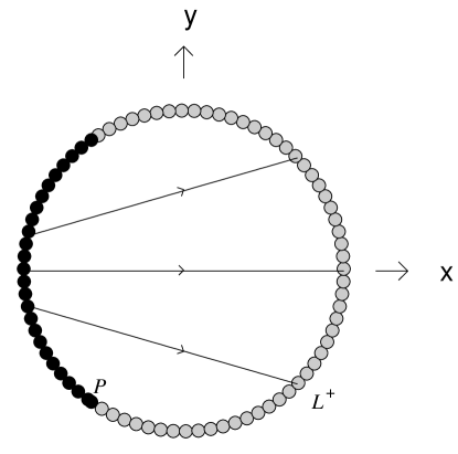
FIG. 1.: Phase portrait of the invariant submanifold $z=0$, corresponding to the case where the RR four–form field strength is trivial and the NS–NS three–form field strength is dynamically important. The line $L^{+}$ represents a line of equilibrium points. Large black dots denote repellers (sources) while grey-filled dots denote attractors (sinks). The point $P$ represents a source in both the two-dimensional and three-dimensional phase spaces.

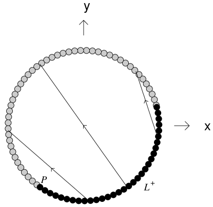
FIG. 2.: Phase portrait of the invariant submanifold $\Omega=0$, corresponding to the case where the NS–NS three–form field strength is trivial and the RR four–form field strength is dynamically important. See also caption to Figure 1.

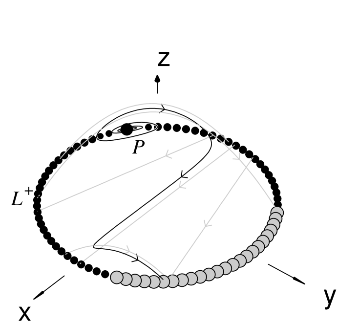
FIG. 3.: Phase diagram of the spatially flat cosmologies when both NS–NS and RR form fields are non–trivial. Note that $L^{+}$ represents a line of equilibrium points. The trajectories in Figures 1 and 2 are depicted in grey in this figure along $z=0$ and $z=1-x^{2}-y^{2}$, respectively. Small black dotes represent saddle points. See also caption to Figure 1.

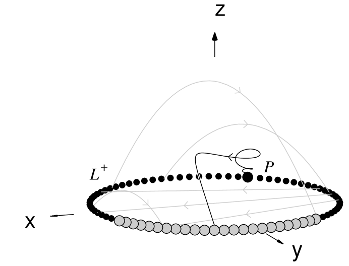
FIG. 4.: An alternative view of a different trajectory in the spatially flat phase space. See also captions to Figures 1 and 3.

The equilibrium set $L^{+}$ represents solutions where the form–fields are trivial and only the dilaton and moduli fields are dynamically important. These are known as the ‘dilaton–moduli–vacuum’ solutions and have an analytical form given by

$$e^{\alpha}=e^{\alpha_{*}}|t|^{\pm h_{*}}$$ (48)

$$e^{\Phi}=e^{\Phi_{*}}|t|^{\pm 3h_{*}-1}$$ (49)

$$e^{\beta}=e^{\beta_{*}}|t|^{\pm\epsilon\sqrt{(1-3h_{*}^{2})/6}},$$ (50)

where $\{\alpha_{*},\Phi_{*},\beta_{*},h_{*}\}$ are constants, and $\epsilon=\pm 1$. Note that the “$-$” solutions in Eq. (48), which are represented by the line $L^{+}$, correspond to $t<0$ and, in the time-reverse case ($\dot{\varphi}<0$), the “$+$” solutions of Eq. (48) correspond to $t>0$.

Let us first consider the dynamics in the invariant submanifold $z=0$, where the NS–NS axion field is non–trivial and the RR four–form field strength vanishes (Fig. 1). These trajectories represent the ‘dilaton–moduli–axion’ solutions discussed in Ref. [17]. The trajectory along $y=0$ corresponds to the solution where the internal dimensions are static. In this case, the universe is initially contracting $(x<0)$, but ultimately bounces into an expansionary phase ($x>0$). The bounce is induced by the two–form potential. It follows from Eq. (14) that the field strength of this antisymmetric tensor field is directly proportional to the volume form of the three–space. This implies that the axion field may be interpreted as a membrane that is wrapped around the spatial hypersurfaces [18]. This membrane resists the initial collapse of the universe and results in a bouncing cosmology. Many solutions exhibit such a bounce, but others collapse to zero volume. These arise when the initial kinetic energy of the modulus field (internal space) is sufficiently high that it can always dominate the kinetic energy of the axion field.

In the other invariant submanifold $(\Omega=0)$, the NS–NS two–form potential is trivial, and the RR three–form potential is dynamical. The cosmological constant term $Q^{2}$ in the effective action (17) may be interpreted as a $0$–form field strength. In a certain sense, this degree of freedom plays a rôle analogous to that of a domain wall [19]. However, in contrast to the membrane associated with the axion field, this ‘domain wall’ resists the expansion of the universe. Thus, the majority of solutions that are initially expanding ultimately recollapse, as shown in Fig. 2. There are some solutions where the internal space is initially evolving sufficiently rapidly that the modulus field dominates the form field and the expansion can proceed indefinitely. Solutions that are initially collapsing do not undergo a bounce.

In both invariant submanifolds, the point $P$ corresponds to an endpoint on the line of sources. In Fig. 1, the reflection of this point in the line $y=0$ represents the opposite end of the line of sources. This point corresponds to a dual solution, where the radius of the internal space is inverted. Thus, the endpoints of the line of sources in the invariant submanifold $z=0$ are related by a scale factor duality.

We may now consider the dynamics in the full three–dimensional phase space, where both the NS–NS two–form potential and RR three–form potential are dynamically significant. Although they are asymptotically negligible, the interplay between these fields has important consequences. The key point is that the RR field causes the universe to collapse, but the NS–NS field has the opposite effect. These two fields therefore compete against one another, as can be seen in Figs. 3 and 4.

The point $P$ is the only source in the system when both form fields are present. Furthermore, it follows from the definitions (33) that it represents the collapsing, isotropic, ten–dimensional cosmology, where $\alpha=\beta$. The four–dimensional dilaton field, $\Phi$, is trivial in this case. As the collapse proceeds, a typical orbit moves upwards in a cyclical fashion until a critical point is reached, where one of the form fields is able to dominate the dynamics. The orbit then shadows the corresponding trajectory in the invariant submanifold $z=0$ or $\Omega=0$. In Fig. 3, the axion field dominates and causes the universe to bounce. By this time, however, the kinetic energy of the modulus field has become significant and the solution ultimately asymptotes to a dilaton–moduli–vacuum solution on $L^{+}$.

All sinks in this phase space correspond to solutions where the internal dimensions are expanding $(y>0)$. There is a particular point where the spatial dimensions spanning the spacetime $M_{4}$ become static in the late–time limit. In general, however, solutions either collapse to zero volume in a finite time or superinflate $(\ddot{\alpha}>0)$ towards a curvature singularity. In this sense, they correspond to pre–big bang cosmologies, since the comoving Hubble radius decreases [15, 20]. However, since the internal space is expanding, it is not clear to what extent this behaviour represents a realistic, four–dimensional inflationary solution.

As discussed above, the time-reversed dynamics of the above class of models is deduced by interchanging the sources and sinks and reinterpreting expanding solutions in terms of contracting ones, and vice–versa. Thus, the late-time attractor for the time–reversed system is the expanding, isotropic, ten–dimensional cosmology located at point $P$.

It is of interest to reinterpret the equilibrium points of the phase space in terms of eleven–dimensional solutions. Since the eleven–dimensional three–form potential is trivial on $L^{+}$, these points represent ‘Kasner’ solutions to eleven–dimensional, vacuum Einstein gravity. Thus, the line $L^{+}$ is analogous to the Kasner ring that arises in the vacuum Bianchi I models of four–dimensional general relativity [16].

For the compactification we have considered, the scale factors in the eleven–dimensional frame are $\{e^{\tilde{\alpha}},e^{\tilde{\beta}},e^{\gamma}\}$, where, from Eq. (6), $\tilde{\alpha}\equiv\alpha-\gamma/2$ and $\tilde{\beta}\equiv\beta-\gamma/2$. The ‘Kasner’ solutions are then given by the power laws $\tilde{\alpha}=\alpha_{0}/\tilde{t}$, $\tilde{\beta}=\beta_{0}/\tilde{t}$ and $\gamma=\gamma_{0}/\tilde{t}$, where $\tilde{t}\equiv\int dt\exp(-\gamma/2)$ and the constants of integration satisfy the constraints $3\alpha_{0}+6\beta_{0}+\gamma_{0}=1$ and $3\alpha_{0}^{2}+6\beta_{0}^{2}+\gamma_{0}^{2}=1$.

These redefinitions imply that the source $P$ corresponds to the ‘Kasner’ solution $(\alpha_{0},\beta_{0},\gamma_{0})=(0,0,1)$. This point represents the Taub form of Minkowski spacetime [16]. The relevance of this solution to the problems associated with the pre–big bang curvature singularity have recently been discussed [7, 8], and it is interesting from an eleven–dimensional point of view that such a simple solution is uniquely selected by the dynamics. The endpoints of the line of sinks on $L^{+}$ correspond to the ‘Kasner’ solutions $(1/2,0,-1/2)$ and $(0,2/7,-5/7)$, respectively, and consequently in both cases a subset of the scale factors are static.

This concludes our discussion of the phase space for the spatially flat cosmologies. In the following Section, we consider the robustness of these models to a number of possible generalizations, including the effects of spatial curvature.

VI Robustness of the Models

A Effects of Spatial Curvature

Although the compactness of the phase space depends on the fact that $k\leq 0$, one can assume arbitrary signs for $k$ in order to determine the local stability of the equilibrium points in the three-dimensional set $u=0$ with respect to curvature perturbations. The eigenvalue associated with $u$ for the equilibrium points $L^{+}$ is always negative. This means that the sinks on $L^{+}$ (i.e., points on $L^{+}$ for $x>-1/\sqrt{3}$ and $\sqrt{2}y>x-1/\sqrt{3}$) remain sinks in the four-dimensional phase-space. In addition, this implies that the point $P$ is now only a saddle; that is, the stability of $P$ is unstable to the introduction of both positive and negative spatial curvature.

Since a portion of $L^{+}$ acts as sinks in the four-dimensional phase space, there exists the global result that the corresponding dilaton–moduli–vacuum solutions (48) (for $3\dot{\alpha}>-\dot{\varphi}$ and $6\dot{\beta}>3\dot{\alpha}-\dot{\varphi}$) will be attracting solutions for the spatially curved models. We may deduce further global results by restricting our attention to the negatively curved models $(k<0)$, in which case the four-dimensional phase space is compact. As discussed above, the point $P$ is a only a saddle point in this extended phase space. Moreover, it follows from the analysis of Section IV that the only attracting equilibrium point is the point $R$. (There is an additional saddle $M$ which will affect the possible intermediate dynamics). This source corresponds to a negatively curved model with a trivial axion field; indeed, it is a power-law, self-similar collapsing solution with non-negligible modulus and RR form–field.

We have been unable to find a monotone function on the extended four-dimensional phase space, but it is plausible that all negatively-curved models evolve from the solution corresponding to the global source $R$ towards the dilaton–moduli–vacuum solutions (on the attracting portion of $L^{+}$). Clearly the curvature is dynamically important at early times.

In the time-reverse case, the solutions asymptote from the non-inflationary dilaton–moduli–vacuum solutions in the past and evolve to the future towards a curvature dominated model; it is plausible that they evolve towards a model which is the time-reversal of the one represented by $R$. Therefore, curvature can also be dynamically important at late times.

B Effects of Generalized Couplings

We now consider a generalization of the effective action (17) given by

$$S=\int d^{4}x\sqrt{-g}\left\{{\rm e}^{-\Phi}\left[R+\left(\nabla\Phi\right)^{2}-6\left(\nabla\beta\right)^{2}-\frac{1}{2}{\rm e}^{2\Phi}\left(\nabla\sigma\right)^{2}-2\Lambda\right]-\frac{1}{2}Q^{2}{\rm e}^{c\beta}\right\},$$ (51)

where $\Lambda$ represents a cosmological constant term and $c$ is an arbitrary constant. The former term may arise through non–perturbative corrections to the string effective action. The motivation for considering an arbitrary coupling of the modulus field to the four–form field strength is that the generality of the dynamics discussed in Section IV (in which $c=-6$) can be investigated. Eq. (51) reduces to the action studied in Ref. [21] when $c=0$.

By invoking the same assumptions as in section III, the action (51) reduces to

$$S=\int dt\left[{\rm e}^{-\varphi}\left(3\dot{\alpha}^{2}-\dot{\varphi}^{2}+6k{\rm e}^{-2\alpha}+6\dot{\beta}^{2}-2\Lambda\right)+\frac{1}{2}{\rm e}^{\varphi+6\alpha}\dot{\sigma}^{2}-Q^{2}{\rm e}^{c\beta+3\alpha}\right]\ ,$$ (52)

and the corresponding field equations can again be derived from this action. In analogy with Eqs. (23) and (28), we introduce a new time variable, $\tau$, defined by

$$\frac{d}{d\tau}=\left(\varphi^{\prime}\right)^{-1}{\rm e}^{-\frac{1}{2}(c\beta+\varphi+3\alpha)}\frac{d}{dt}\ ,$$ (53)

and the new reduced variable

$$v=\frac{2\Lambda{\rm e}^{-(3\alpha+\varphi+c\beta)}}{(\varphi^{\prime})^{2}}.$$ (54)

From these definitions and the reduced variables defined earlier, we obtain a five-dimensional system of ordinary differential equations for the reduced (dimensionless) variables after eliminating the variable $\Omega$ that is now defined by $\Omega\equiv 1-x^{2}-y^{2}-z-u-v$. Since $\rho\geq 0$, all of the dimensionless variables are bounded for the models with $k\leq 0$ and $\Lambda>0$, where the physical state space is defined by $0<\left\{x^{2},y^{2},z,u,v\right\}<1$, and a global analysis is therefore possible in this case. Including the boundaries $\Omega=0$, $z=0$, $u=0$ and $v=0$ leads to a compact state space.

We can analyse these models and obtain qualitative information about the dynamics in an analogous way to that done in section III [22]. The equilibrium set $L^{+}$: $x^{2}+y^{2}=1,z=u=v=0$ still exists, and since the eigenvalues associated with ($u$ and) $v$ are (both) negative, part of $L^{+}$ will act as sinks and the non-hyperbolic point $x=-1/\sqrt{3},y=-\sqrt{2/3},z=u=v=0$ is clearly a saddle. These are local results and are valid in all cases.

There also exists an attracting equilibrium point $W$:

$$x=-\sqrt{3}\left(12+c^{2}\right)D^{2}\ ,\ y=8c\sqrt{6}D^{2}\ ,\ z=-192CD^{4}\ ,\ u=v=0\ ,$$ (55)

with eigenvalues

$$-2CD^{2}\ ,\ -(C\pm\sqrt{C(17c^{2}+924)})D^{2}\ ,-4(12+c^{2})D^{2}\ ,\ -6(12+c^{2})D^{2}\ ,$$

where $C\equiv(c+6)(c-6)$ and $D^{-2}\equiv 108+c^{2}$. Note that this point corresponds to an exact self-similar collapsing cosmological solution with non–trivial modulus and four–form fields. The value of $\Omega$ as a function of $c$ is given by

$$\Omega=\frac{-2C(60+c^{2})}{(108+c^{2})^{2}},$$ (56)

which implies that $-6\leq c\leq 6$ in order for $\Omega\geq 0$. When $c=\pm 6$, the point $W$ is a part of the equilibrium set $L^{+}$; in fact, it becomes just the non-hyperbolic point $P$ discussed previously. Note that it is also a part of the invariant submanifold $cx-6\sqrt{2}y+\sqrt{3}c=0;u=v=0$, which generalizes the invariant submanifold $K$ defined in Eq. (43).

There are two non-flat ($u\neq 0$) vacuum equilibrium points with a vanishing cosmological constant $v=0$, one of which is a source and the other a saddle. There is also a non-hyperbolic vacuum equilibrium point with a non-vanishing cosmological constant ($v=1$) with $x=y=z=u=0$, which appears to be a source. In addition, we can find monotone functions in the boundary submanifolds; indeed, the boundary $\Omega=u=v=0$ and the boundary submanifold $z=u=v=0$ can be solved exactly in terms of the variables of the state space. Exact solutions of the equations of motion for particular values of $c$ can also be found.

However, the primary motivation for these comments is to emphasize two important points regarding the very interesting dynamics of the M–theory cosmologies studied earlier. First, we note that the conclusions obtained for the spatially curved models are robust when additional physical fields (e.g., a $\Lambda$ term) are included. Second, and perhaps more importantly, we see that the value $c=-6$ is a bifurcation value in the analysis of general models with arbitrary coupling, $c$. In this context, therefore, the M-theory cosmological models we have studied exhibit rather unique dynamics.

VII Discussion

In this paper we have presented a complete dynamical analysis of spatially flat, four–dimensional cosmological models derived from the M-theory and type IIA string effective actions. We have shown that models generically spiral away from a source $P$, undergoing bounces due to the interplay between the NS-NS two-form potential and the RR three-form potential. Eventually, they evolve towards dilaton-moduli-vacuum solutions with trivial form fields (corresponding to the sinks on $L^{+}$). We note the important dynamical result that $\varphi^{\prime}$ is monotonic.

Thus, the form fields that arise as massless excitations in the type IIA superstring spectrum, or equivalently from the three–form potential of eleven–dimensional supergravity, may have important consequences in determining initial and final conditions in string and M–theory cosmologies, even though they are dynamically negligible in the early– and late–time limits. In particular, the point $P$ is the only source in the system. It can be interpreted in the string context as the isotropic, ten-dimensional solution. Alternatively, it represents the Taub form of flat space when viewed in terms of eleven–dimensional variables.

When the effects of spatial curvature are included, we obtained the local result that the point $P$ becomes a saddle. On the other hand, the dilaton-moduli-vacuum solutions with trivial form fields are generic attracting solutions. In the analysis of the negatively-curved models, we found that the early time attractor (the source $R$) has non-zero curvature, implying that spatial curvature is dynamically important at early times in these examples.

This work can be generalized in a number of ways. We considered a specific compactification from eleven to four dimensions, where the topology of the internal dimensions was assumed to be a product space consisting of a circle and an isotropic six–torus. We emphasize, however, that the analysis also applies to compactifications on a Calabi–Yau three–fold since the gauge fields arising from the higher–dimensional metric have been ignored [7]. The qualitative analysis may be readily extended to compactifications on a general, rectilinear torus $S^{1}\times\ldots\times S^{1}$. After suitable redefinitions of the additional moduli fields that subsequently arise, the dimensionally reduced action can be expressed precisely in the form of Eq. (17), with the inclusion of a set of massless scalar fields in the NS–NS sector. In particular, the compactification on $T^{4}\times T^{2}\times S^{1}$, where $T^{n}$ represents the isotropic $n$–torus, is relevant to compactifications involving the four–dimensional space $K3$ [23]. This space has played an important rôle in establishing various string dualities [3]. It is the simplest four–dimensional, Ricci–flat manifold after the torus [24] and may be approximated by the orbifold $K3\approx T^{4}/{\rm Z}_{2}$ [25].

Moreover, the effects of spatial anisotropy in the spacetime $M_{4}$ can also be considered by introducing two, uncoupled moduli fields into the NS–NS sector of the reduced action (18). In this context, such fields parametrize the shear in the cosmologies. When these fields are non–trivial, the models represent the class of isotropic curvature cosmologies and correspond to Bianchi type I, V and IX universes [21, 26]. It would be interesting to consider these generalizations further.

- [1] M. B. Green, J. H. Schwarz, and E. Witten, Superstring Theory, in 2 vols., (Cambridge University Press, Cambridge, 1987); J. Polchinski, String Theory, in 2 vols., (Cambridge University Press, Cambridge, 1998).
- [2] E. Witten, Nucl. Phys. B443, 85 (1995).
- [3] A. Sen, hep-th/9802051.
- [4] P. Townsend, Phys. Lett. B350, 184 (1995).
- [5] A. Lukas, B. A. Ovrut, and D. Waldram, hep-th/9806022; A. Lukas, B. A. Ovrut, and D. Waldram, hep-th/9812052; H. S. Reall, Phys. Rev. D59, 103506 (1999); K. Benakli, Int. J. Mod. Phys. D8, 153 (1999); K. Benakli, Phys. Lett. B447, 51 (1999).
- [6] H. Lu, S. Mukherji, and C.N. Pope, hep-th/9612224; A. Lukas, B. A. Ovrut, and D. Waldram, Nucl. Phys. B495, 365 (1997); H. Lu, S. Mukherji, C. N. Pope, and K. -W. Xu, Phys. Rev. D55, 7926 (1997); A. Lukas, B. A. Ovrut, Phys. Lett. B437, 291 (1998); H. Lu, J. Maharana, S. Mukherji, and C. N. Pope, Phys. Rev. D57, 2219 (1998); A. Lukas, B. A. Ovrut, and D. Waldram, Nucl. Phys. B509, 169 (1998); M. Bremer, M. J. Duff, H. Lu, C. N. Pope, and K. S. Stelle, Nucl. Phys. B543, 321 (1999); M. J. Duff, P. Hoxha, H. Lu, R. R. Martinez–Acosta, and C. N. Pope, Phys. Lett. B451, 38 (1999); S. W. Hawking and H. S. Reall, Phys. Rev. D59, 023502 (1999).
- [7] N. Kaloper, I. I. Kogan, and K. A. Olive, Phys. Rev. D57, 7340 (1998); Erratum, ibid. D60, 049901 (1999).
- [8] A. Feinstein and M. A. Vazquez–Mozo, hep-th/9906006.
- [9] E. Cremmer, B. Julia, and J. Scherk, Phys. Lett. B76, 409 (1978); E. Cremmer and B. Julia, Phys. Lett. B80, 48 (1978); E. Cremmer and B. Julia, Nucl. Phys. B156, 141 (1979).
- [10] L. Castellani, P. Fre, F. Giani, K. Pilch, and P. van Nieuwenhuizen, Ann. Phys. 146, 35 (1983).
- [11] I. C. Campbell and P. C. West, Nucl. Phys. B243, 112 (1984); F. Giani and M. Pernici, Phys. Rev. D30, 325 (1984); M. Huq and M. A. Namazie, Class. Quantum Grav. 2, 293 (1985); Erratum, ibid. 2, 597 (1985).
- [12] A. Shapere, S. Trivedi, and F. Wilczek, Mod. Phys. Lett. A6, 2677 (1991); A. Sen, Mod. Phys. Lett. A8, 2023 (1993).
- [13] P. G. O. Freund and M. A. Rubin, Phys. Lett. B97, 233 (1980); F. Englert, Phys. Lett. B119, 339 (1982).
- [14] A. A. Tseytlin, Int. J. Mod. Phys. D1, 223 (1991).
- [15] G. Veneziano, Phys. Lett. B265, 287 (1991).
- [16] J. Wainwright and G. F. R. Ellis, Dynamical Systems in Cosmology (Cambridge University Press, Cambridge, 1997).
- [17] E. J. Copeland, A. Lahiri, and D. Wands, Phys. Rev. D50, 4868 (1994).
- [18] N. Kaloper, Phys. Rev. D55, 3394 (1997).
- [19] H. Lu, C. N. Pope, E. Sezgin, and K. S. Stelle, Nucl. Phys. B456, 669 (1995); H. Lu, C. N. Pope, E. Sezgin, and K. S. Stelle, Phys. Lett. B371, 46 (1996); M. Cvetic and H. H. Soleng, hep-th/9604090; P. M. Cowdall, H. Lu, C. N. Pope, K. S. Stelle, and P. K. Townsend, Nucl. Phys. B486, 49 (1997).
- [20] M. Gasperini and G. Veneziano, Astropart. Phys. 1, 317 (1993).
- [21] A. P. Billyard, A. A. Coley, and J. E. Lidsey, gr-qc/9907043; A.P. Billyard, A. A. Coley and J. E. Lidsey, “Qualitative Analysis of Isotropic Curvature String Cosmologies” (1999).
- [22] A. P. Billyard, Ph. D Thesis (1999).
- [23] M. J. Duff, B. E. W. Nilsson, and C. N. Pope, Phys. Lett. B129, 39 (1983); H. Lu, C. N. Pope, and K. S. Stelle, Nucl. Phys. B548, 87 (1999).
- [24] P. S. Aspinwall, hep-th/9611137.
- [25] D. N. Page, Phys. Lett. B80, 55 (1978); G. W. Gibbons and C. N. Pope, Commun. Math. Phys. 66, 267 (1979).
- [26] M. A. H. MacCallum, Cargese Lectures in Physics ed. E. Schatzman (Gordon and Breach, New York, 1973).