Casimir’s energy of a conducting sphere and of a dilute dielectric ball

Abstract

In this paper we sum over the spherical modes appearing in the expression for the Casimir energy of a conducting sphere and of a dielectric ball (assuming the same speed of light inside and outside), before doing the frequency integration. We derive closed integral expressions that allow the calculations to be done to all orders, without the use of regularization procedures. The technique of mode summation using a contour integral is critically examined.

Departments of Applied Mathematics and Physics, Technion, 32000 Haifa, Israel

1 Introduction

The Casimir effect is a remarkable consequence of QFT, exhibiting the reality of the zero point energy of the vacuum. This energy can be made manifest by studying its dependence on various constraints imposed on the electromagnetic field. Casimir’s [1] original analysis for parallel plates yielded a force per unit area ($\hbar=c=1$)

$$-\frac{\pi^{2}}{240a^{4}}$$ (1)

between two conducting plates separated by a distance $a$. The Casimir force for a conducting spherical shell was first calculated by Boyer [2]. The result was indeed puzzling: the force turned out to be repulsive. This was surprising in view of the connection between Casimir’s force and Van-Der-Waals forces which are attractive. This phenomenon may be also related to a fundamental difference between the spherical Casimir problem and that of the plates: expansion of the sphere changes the distances between the points on the shell itself, and thus it is not clear weather the Casimir energy (associated with interaction among different patches on the shell) and electromagnetic the self energy of the shell can be separated [3]. It is not surprising, however, that this in turn called for a large number of subsequent calculations by various techniques [4, 5, 6, 7, 8]. There has been some controversy concerning the regularization procedures used in the calculations, bearing, for example on the relevance of Casimir’s effect to sonoluminescence [10, 11, 12, 13]. Since the repulsive nature of the Casimir force for spherical boundary conditions is somewhat counterintuitive it seems of importance to justify it more rigorously.

We define the Casimir energy of a conducting sphere as follows: Let $\omega_{n}^{(a,R)}$ be the eigenmodes of the electromagnetic field inside two concentric spherical shells of radii $a$ and $R$ $(a<<R)$, where a large sphere of radius $R$ is introduced as an infrared cutoff in order to discretize the spectrum outside the smaller sphere as well as inside it. The zero point energy of this system, namely $\frac{1}{2}\sum_{n}\omega_{n}^{(a,R)}$ is a divergent sum. The Casimir energy is then defined as the zero point energy difference between our configuration and a configuration where the inner sphere is of radius $b$ ($a<<b<R$) [14]

$$E_{C}=\lim_{\sigma\rightarrow 0}\lim_{b\rightarrow\infty}\lim_{R\rightarrow\infty}\frac{1}{2}\sum_{n}\big{(}e^{-\sigma\omega_{n}^{(a,R)}}\omega_{n}^{(a,R)}-e^{-\sigma\omega_{n}^{(b,R)}}\omega_{n}^{(b,R)}\big{)}$$ (2)

Here $e^{-\sigma\omega_{n}}$ is an exponential regulator. We show that if the subtraction procedure is done properly, no further regularization (apart from keeping the naive exponential regulator, required to make the sums well defined, and the subtraction) is actually needed. In the sequel , we follow closely the procedure of mode summation using a contour integral, but our main result can also be applied to the Green’s function method [6].

Most of the calculations have been carried out for the case of a conducting sphere and of a dielectric ball having the same speed of light inside and outside, that is, $\sqrt{\epsilon\mu}=\sqrt{\epsilon^{\prime}\mu^{\prime}}=1$ [15], where $\epsilon,\mu$ are the permittivity and permeability of the medium surrounding a ball of radius $a$, and $\epsilon^{\prime},\mu^{\prime}$ are the permittivity and permeability inside the ball. It has been shown that the Casimir energy in the latter case is given by [7, 17]

$$E=-\frac{1}{2\pi a}\int_{-\infty}^{\infty}dye^{iy\delta}\sum_{l=1}^{\infty}(l+\frac{1}{2})x\frac{d}{dx}\ln{(1-\xi^{2}{(s_{l}e_{l})^{\prime}}^{2})}$$ (3)

where $x=|y|,\nu=l+\frac{1}{2}$ and

$$\xi=\frac{\mu-\mu^{\prime}}{\mu+\mu^{\prime}};\quad\delta=\frac{\tau}{a}$$ (4)

$$s_{l}(x)=ixj_{l}(ix)=\sqrt{\frac{\pi x}{2}}e^{-\frac{i\pi\nu}{2}}J_{\nu}(ix)$$ (5)

$$e_{l}(x)=ixh_{l}^{(1)}(ix)=i\sqrt{\frac{\pi x}{2}}e^{\frac{i\pi\nu}{2}}H^{1}_{\nu}(ix)$$ (6)

and in the end of the calculation the regulator $\delta$ is taken to zero. In the case $\xi=1$, (3) is equivalent to the expression for the energy of a conducting sphere in vacuum.

In order to evaluate (3), extensive use has been made of uniform asymptotic approximations of the modified Bessel functions $s_{l}(x)$ and $e_{l}(x)$. Our evaluation refrains from the use of these asymptotics, which, although very convenient in actual calculations, somewhat obscures the nature of the expression (3). By studying the $l$-sum of this expression before making the frequency integration, using simple orthogonality considerations we arrive at a general formula for sums of the form $\sum(2l+1)(s_{l}e_{l})^{n}$. We show that to first order in $\xi^{2}$ the integrand consists of a constant term (which is independent of the radius) and a function of $a$. Thus the divergence appearing in the evaluation of (3) is due to integration of this constant over all frequencies. This divergence was already pointed out by Candelas [18], however, this constant term would not be present if subtraction of the Casimir energy of a large radius sphere is done properly.

We start by carefully reviewing the procedure of mode summation, using a contour integral, as was done in some previous works [9, 7, 17]. In this method the final integration is carried along the imaginary axis. Justification for the neglect of the part of the contour away from this axis will be given, by concrete estimates, taking into account the existence of an infinite number of poles of the integrand on the real axis.

2 Mode summation for conducting spherical shells

In order to make the discussion well defined we investigate the following situation [19]: A conducting sphere of radius $a$ is placed (concentrically) inside a large conducting sphere of radius $R$. Using multipole expansion [20] the appropriate modes of the electromagnetic fields can be found, through the boundary conditions $B_{r}=0$ and $E_{\theta,\varphi}=0$ on the shells. The eigenmodes are given as solutions to the equations:
(I) Inside the inner sphere

$$\Delta_{l}^{(1)}\equiv j_{l}(\omega a)=0$$ (7)

$$\Delta_{l}^{(2)}\equiv{d\over dr}[rj_{l}(\omega r)]\biggr{|}_{r=a}=0$$ (8)

II) Between the shells

$$\Delta_{l}^{(3)}\equiv j_{l}(\omega R)n_{l}(\omega a)-j_{l}(\omega a)n_{l}(\omega R)=0$$ (9)

$$\Delta_{l}^{(4)}\equiv{d\over dr}[rj_{l}(\omega r)]\biggr{|}_{r=a}{d\over dr}[rn_{l}(\omega r)]\biggr{|}_{r=R}-{d\over dr}[rj_{l}(\omega r)]\biggr{|}_{r=R}{d\over dr}[rn_{l}(\omega r)]\biggr{|}_{r=a}=0$$ (10)

Where equations (7),(9) refer to transverse electric modes, and (8),(10) refer to transverse magnetic modes. Next we define the function [19]

$$\Delta_{l}(\omega;a,R)=\omega^{2}\Delta_{l}^{(1)}\Delta_{l}^{(2)}\Delta_{l}^{(3)}\Delta_{l}^{(4)}$$ (11)

$\Delta_{l}$ is an analytic function, whose positive real zeros are the modes of the electromagnetic field inside the concentric spheres.

In order to sum over the modes of a given $l$, we use the identity [7, 9]

$$\sum_{n=1}^{N}\omega_{(n,l)}e^{-\sigma\omega_{(n,l)}}={1\over 2\pi i}\oint_{C_{N}}dze^{-\sigma z}z{d\over dz}\ln\Delta_{l}(z)$$ (12)

Here $C_{N}$ is a contour which encircles the zeros $\omega_{(1,l)},..\omega_{(N,l)}$ of $\Delta_{l}$ . Since there is an infinite number of modes for each $l$, this sum will diverge if we take $N$ to infinity and $\sigma$ to zero. As usual, the Casimir energy should be identified with that obtained after the subtraction of the zero point energy of the unconstrained “free” system [14],

$$\Delta E(\sigma,b,R)=\lim_{N\rightarrow\infty}{1\over 2\pi i}\sum_{l=1}^{\infty}(l+{1\over 2})\oint_{C_{N}}dze^{-\sigma z}zF_{l}$$ (13)

Where

$$F_{l}(z;a,b,R)=\Big{(}{d\over dz}\ln\Delta_{l}(z;a,R)-{d\over dz}\ln\Delta_{l}(z;b,R)\Big{)}.$$ (14)

The Casimir energy is then given by the limit:

$$E_{C}=\lim_{\sigma\rightarrow 0}\lim_{b\rightarrow\infty}\lim_{R\rightarrow\infty}\Delta E(\sigma,b,R).$$ (15)

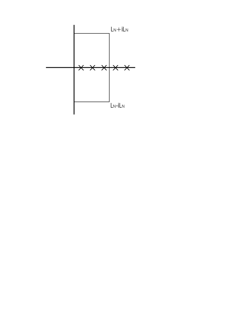
Figure 1: A rectangular contour in the complex plane.

After the limits $R\rightarrow\infty$ and $b\rightarrow\infty$ are taken the remaining expression will have no reference to $R$ and $b$. Removal of the ultra-violet cut off by taking the limit $\sigma\rightarrow 0$ is done in the end of the derivation, after insuring convergence for all values of $b$ and $R$.

In order to make the evaluation of the contour integrals easier we take rectangular contours of side $L_{N}$ (Fig. 1). Our first aim is to carry the entire integration along the imaginary axis, by showing that the contribution of the part of the contour away from it vanishes as $L_{N}$ goes to infinity. The justification of this neglect, however, is not obvious, since the integrand in (13) has infinitely many singularities along the real axis, which become ever denser as $R\rightarrow\infty$. This follows from the property that for any finite $R$ there is an infinite number of field modes, and subsequently there is a corresponding infinite number of poles of $z{d\over dz}\ln\Delta_{l}(z,b,R)$ along the real axis. Even after taking the limit $R\rightarrow\infty$ the spectrum will still consist of a discrete set (eigenmodes inside the inner shell) imbedded in a continuum part. Indeed, let us examine the behavior of $\Delta_{l}(\omega;a,R)$ for large arguments $\omega$. Using the asymptotic behavior [20]

$$j_{l}\rightarrow\frac{1}{x}\sin(x-\frac{l\pi}{2})$$ (16)

$$n_{l}\rightarrow-\frac{1}{x}\cos(x-\frac{l\pi}{2})$$ (17)

we obtain

$$\Delta_{l}(\omega;a,R)\rightarrow\frac{1}{2a^{2}R\omega}\sin(2\omega a-l\pi)\sin^{2}(\omega(R-a))$$ (18)

Thus for large arguments the modes behave as $\frac{n\pi}{2a}$ or $\frac{n\pi}{2(R-a)}$ where $n$ is an integer. (Note that the density of modes for large frequencies is similar to that appearing in the one dimensional version of the standard Casimir effect for parallel conducting plates separated by a distance $a$ inside a large box of length $R$.) Let us examine the behavior of the integrand for large values of $|\omega|$. Substituting the asymptotics (18), we show that the integral on a contour that does not pass through one of the poles, decays exponentially fast. The integrand is then simply:

$$F_{l}(\omega;a,b,R)=2\big{(}a(\cot(2\omega a-l\pi)-\cot(\omega(R-a)))+$$

$$R(\cot(\omega(R-a))-\cot(\omega(R-b)))+$$

$$b(\cot(\omega(R-a))-\cot(2\omega b-l\pi))\big{)}$$ (19)

It is easy to check that for ${\rm Im}~{}\omega\rightarrow\infty$ and any real $A,B$,

$$|\cot(A\omega)-\cot(B\omega)|=O(e^{-2min(A,B){\rm Im}~{}\omega})$$ (20)

Thus on the upper and lower parts of the contour (${\rm Im}~{}z=\pm L_{N}$) the integral is bounded by:

$$\left|\int_{0}^{L_{N}}(iL_{N}+z)F_{l}(iL_{N}+z)dz\right| \leq \int_{0}^{L_{N}}|iL_{N}+z|12Re^{-4aL_{N}}dz$$ (21)

$$\leq 18L_{N}^{2}Re^{-4aL_{N}}$$

The part of the contour with ${\rm Re}~{}z=L_{N}$ can be evaluated as follows. First we prove that integrals of the form

$$\int_{-L}^{L}e^{-\sigma(L+ix)}(L+ix)\cot(kL+ikx)dx$$ (22)

decay exponentially as $L\rightarrow\infty$ as long as we avoid the poles (i.e. $kL\neq n\pi$). Choose $L_{N}=\frac{N\pi}{k}+\frac{\pi}{2k}$; then we have

$$\left|\int_{-L_{N}}^{L_{N}}e^{-\sigma(L_{N}+ix)}(L_{N}+ix)\cot(kL_{N}+ikx)dx\right|=$$

$$e^{-\sigma L_{N}}\left|\int_{-L_{N}}^{L_{N}}e^{-i\sigma x}(L_{N}+ix)\tanh(kx)dx\right|\leq 3L_{N}^{2}e^{-\sigma L_{N}}$$ (23)

This is enough to ensure exponential decay for any $kL\neq n\pi$, since we can shift the right side from $L_{N}$ to $L_{N}-\frac{\pi}{2k}<L<L_{N}+\frac{\pi}{2k}$ at a “cost” of less then $\frac{\pi}{k}L_{N}^{2}e^{-\sigma L_{N}}$. Combining estimates (21) and (23) we see that integration over the part of the contour with ${\rm Re}~{}z>0$ decays exponentially like $e^{-\sigma L_{N}}$. In the limit $L_{N}\rightarrow\infty$ we obtain the desired equality:

$$\sum_{n=1}^{\infty}\omega_{(n,l)}e^{-\sigma\omega_{(n,l)}}=\int_{-i\infty}^{i\infty}dze^{-\sigma z}z{d\over dz}\ln\Delta_{l}(z).$$ (24)

In the limit of large $R$, we have on the imaginary axis (${\rm Re}~{}\omega=0$)

$$\Delta_{l}^{(3)}\Delta_{l}^{(4)}(\omega)=\frac{1}{2\omega}\sin(2\omega R-l\pi){h_{l}}^{(1)}(\omega a){d\over d\omega}[\omega{h_{l}}^{(1)}(\omega a)],$$ (25)

where

$$h_{l}^{(1)}(\omega)=j_{l}(\omega)+in_{l}(\omega).$$ (26)

After summation over the $l$ index and some algebraic manipulation we obtain [7]:

$$E_{c}=-{1\over\pi}\lim_{\sigma\rightarrow 0}\lim_{b\rightarrow\infty}\sum_{l=1}^{\infty}(l+{1\over 2})\int^{\infty}_{0}d\omega e^{-i\sigma\omega}\omega{d\over d\omega}\biggr{(}ln\big{[}1-{(s_{l}e_{l}(a\omega))^{\prime}}^{2}\big{]}$$ (27)

$$-ln\big{[}1-{(s_{l}e_{l}(b\omega))^{\prime}}^{2}\big{]}\biggr{)}$$

in agreement with (3). Note that the usual derivation of (3) involves a rescaling $x=a\omega$. In our derivation we avoided this step and as a result, were able to identify the term in the $\omega$-integral which is independent of the radius, and hence makes (3) divergent.

3 Expansion in $\xi^{2}$: first order

In the previous section we reviewed the derivation of the expression for the Casimir energy of a conducting sphere. The Casimir energy of a dielectric ball, under the condition $\sqrt{\epsilon\mu}=\sqrt{\epsilon^{\prime}\mu^{\prime}}=1$ [7, 17] can be calculated at no further cost by repeating essentially the same steps as in the conducting case. Furthermore, it was shown [16], that calculations in this case, will yield the same result independent of the regularization used. From now on this will be the setting, with $\xi=1$ (4) corresponding to the previous section. We now show that the sum over the angular index $l$ in (3) can be carried out before doing the integration over the frequencies. We assume $\xi^{2}$ small, and expand the logarithm in (3) in powers of $\xi^{2}$. The first term in this expansion is

$$-\xi^{2}\sum_{l=1}^{\infty}(l+\frac{1}{2})x\frac{d}{dx}{(s_{l}e_{l})^{\prime}}^{2}.$$ (28)

It turns out that the sum over $l$ in (28) can be done exactly. To this end, note the following identity, which can easily be obtained from the expansion of the Helmholtz propagator in spherical coordinates [21] using relations (5) and (6),

$$D(x,\rho)\equiv\frac{\tilde{r}rxe^{-x\rho}}{\rho}=\sum_{l=0}^{\infty}(2l+1)s_{l}(x\tilde{r})e_{l}(xr)P_{l}(\cos\theta)$$ (29)

$$\rho=\sqrt{\tilde{r}^{2}+r^{2}-2\tilde{r}r\cos\theta}$$ (30)

where $\theta$ is the angel between two vectors of lengths $r$ and $\tilde{r}$.

The following can, of course, be carried out for arbitrary $\tilde{r}$ and $r$ . This should be useful in the more general case where $\sqrt{\epsilon\mu}\neq\sqrt{\epsilon^{\prime}\mu^{\prime}}$, since the expressions appearing in that case involve combinations of $s_{l}(x^{\prime})e_{l}(x)$ where $x=\sqrt{\epsilon\mu}\omega$ and $x^{\prime}=\sqrt{\epsilon^{\prime}\mu^{\prime}}\omega$ [10], but in the present case $r=\tilde{r}=1$ is just what we need. Using the orthogonality relations of the $P_{l}$’s

$$\int_{-1}^{1}P_{l}(x)P_{j}(x)dx=\delta_{lj}\frac{2}{2l+1}$$ (31)

and substituting d$\cos\theta=-\rho d\rho$ we obtain the identity

$$\sum_{l=0}^{\infty}(2l+1){(s_{l}e_{l})^{\prime}}^{2}=\frac{1}{2}\int_{0}^{2}(\frac{\partial}{\partial x}{D(x,\rho))}^{2}\rho d\rho$$ (32)

Thus the sum over $l$ in (28) can be carried out, as promised, and we find

$$-\frac{\xi^{2}}{2}(\frac{1}{2}\int_{0}^{2}x\frac{d}{dx}(\frac{d}{dx}{D(x,\rho))}^{2}\rho d\rho-x\frac{d}{dx}{(s_{0}e_{0})^{\prime}}^{2})=$$

$$\frac{\xi^{2}}{2}(\frac{1}{2}-\frac{1}{2}e^{-4x}(1-2x)^{2}+4xe^{-4x})$$ (33)

We note the appearance of a term $\frac{\xi^{2}}{4}$ which is independent of $x$ and thus causes (3) to diverge. We dispose of it by subtracting from (33) the appropriate term corresponding to a radius $b$ and taking the limit $b\rightarrow\infty$, and obtain the density

$$G(\omega)\equiv\frac{\xi^{2}}{8\pi}e^{-4a|\omega|}(1+4a|\omega|+4a|\omega|^{2})$$ (34)

Thus, finally the first term in the $\xi^{2}$ expansion of (3) can be analytically derived. The energy to this order is

$$E=\int_{-\infty}^{\infty}{d\omega G(\omega)}=\frac{\xi^{2}}{2a}\frac{5}{16\pi}+O(\xi^{4})=\frac{\xi^{2}}{2a}0.0994718+O(\xi^{4}).$$ (35)

$\xi=1$ corresponds to the case of a conducting sphere. It turns out that this result has already been derived for a conducting sphere, by Balian and Duplantier [5] using a multiple scattering formalism, which may be applied in the case of conducting boundaries of arbitrary shape. Using a Green’s function method, Milton, DeRaad and Schwinger [6] evaluated the Casimir Energy for a conducting sphere, Numerically, to be $\frac{1}{2a}0.092353$. This is in accordance with our calculation, since the next term in the $\xi^{2}$ expansion of (3) may be evaluated using the Debye asymptotic expansion of Bessel functions to be $-\frac{1}{2a}0.007$. However, for a dilute sphere ($\xi<<1$) our result is the exact one. Note that our result was obtained using only subtraction of energies, which is in the definition of the Casimir energy. No further regularization of the expression (28) was necessary.

4 An integral expression for higher orders in $\xi^{2}$

Generalization of the method we developed in the previous section to higher orders in $\xi^{2}$, is possible. To this end, we derive a general formula for sums of the form $\sum_{l}(l+1/2)a_{l}^{n}$, for arbitrary power $n$, and coefficients $a_{l}$, when the function $f(x)=\sum_{l}(l+1/2)a_{l}P_{l}(x)$ is known. Let us first introduce the following transform

$$f(x)\rightarrow\widehat{f}(x,y)=\frac{1}{\pi}\int_{0}^{\pi}dtf\big{(}xy-\sqrt{(1-x^{2})(1-y^{2})}\cos t\big{)}$$ (36)

This transform has the simple property that if $f(x)=\sum_{l}a_{l}P_{l}(x)$ then

$$\widehat{f}(x,y)=\sum_{l}a_{l}P_{l}(x)P_{l}(y)$$ (37)

To see this, we write $x=\cos\alpha$, $y=\cos\beta$ and consider the following well known addition formula:

$$P_{l}(\cos\gamma)=P_{l}(\cos\alpha)P_{l}(\cos\beta)+2\sum_{m=1}^{l}P_{l}^{m}(\cos\alpha)P_{l}^{m}(\cos\beta)\cos(m(\theta-\varphi))$$ (38)

where $\gamma$ is the angle between two unit vectors with spherical coordinates $(\alpha,\theta)$ and $(\beta,\varphi)$, that is

$$\cos\gamma=\cos\alpha\cos\beta+\sin\alpha\sin\beta\cos(\theta-\varphi)$$ (39)

setting $\theta=t$ and $\varphi=0$, we obtain:

$$f(\cos\alpha\cos\beta-\sin\alpha\sin\beta\cos t)=\sum_{l}a_{l}P_{l}(\cos\gamma)=$$

$$\sum_{l}a_{l}\big{[}P_{l}(\cos\alpha)P_{l}(\cos\beta)+2\sum_{m=1}^{l}P_{l}^{m}(\cos\alpha)P_{l}^{m}(\cos\beta)\cos(mt)\big{]}$$ (40)

Integrating over $t$, we eliminate all the terms containing $\cos t$, and are left with $\sum_{l}a_{l}P_{l}(x)P_{l}(y)$ as claimed. Using (37) and (31) repeatedly, we obtain

$$\sum_{l=0}^{\infty}(l+1/2)a_{l}^{n}=\int_{-1}^{1}\prod_{j=1}^{n-1}dx_{j}\big{(}f(x_{1})\underbrace{\widehat{f}(x_{1},x_{2})\cdot...\widehat{f}(x_{n-2},x_{n-1})}_{(n-2)terms}f(x_{n-1})\big{)}$$ (41)

Thus, for example, we can cast the $\xi^{4}$ term in the expansion of (3) in the form:

$$\frac{-\xi^{4}}{32\pi^{3}a}\Big{(}\int_{0}^{\infty}dx\int_{-1}^{1}d\cos\theta_{1}d\cos\theta_{2}d\cos\theta_{3}\int_{0}^{\pi}dt_{1}dt_{2}\prod_{i=1}^{4}\frac{d}{dx}D(x,\rho_{i})-\pi^{2}\Big{)}$$ (42)

where

$$\rho_{1}=\sqrt{2-2\cos\theta_{1}}\,\,\,;\,\rho_{2}=\sqrt{2-2(\cos\theta_{1}\cos\theta_{2}-\sin\theta_{1}\sin\theta_{2}\cos t_{1})}$$

$$\rho_{3}=\sqrt{2-2(\cos\theta_{2}\cos\theta_{3}-\sin\theta_{2}\sin\theta_{3}\cos t_{2})}\,\,\,;\,\rho_{4}=\sqrt{2-2\cos\theta_{3}}$$ (43)

It is not difficult to check that (42) indeed converges but, unfortunately, we have not succeeded in integrating it analytically.

5 Discussion

In this paper we developed and used a novel method appropriate for calculations of the Casimir energy for spherical boundary conditions. Although the use of the asymptotic Debye approximation is very convenient, we have shown that it is possible to make a direct summation over angular modes using the expansion of the Helmholtz propagator in spherical harmonics. This method can be applied to obtain closed integral representations for any order in the $\xi^{2}$ expansion of the Casimir energy (3). The $\xi^{2}$ order was explicitly calculated to be $\frac{5\xi^{2}}{32a\pi}$, this result is within $0.13\%$ of results obtained via the Debye approximations [17], demonstrating their high accuracy. Higher orders in $\xi^{2}$ however, still remain in integral form.

Our method should be applicable to other sums of the type (28) and variations on them [10], which are common in the calculations for spherical boundaries, in order to get more regularization independent results. The fact that summation using angular integrals over the propagator of the Helmholtz equation through (41) can be done to all orders, reflects the relation between the mode summation technique and calculations using Green’s function. This can be seen for the case of conducting boundaries in the multiple scattering formalism [5]. It would be illuminating to reveal the connections between our method and other methods of calculation in the dielectric case, involving summation over dipoles, such as calculations of the Casimir energy using the statistical mechanics partition function as was performed by Høye and Brevik [22].

References

- [1] H. B. G. Casimir, Proc. Koninkl. Ned. Akad. Wetenschap. 51, 793 (1948).
- [2] T. H. Boyer, Phys. Rev. 174, 1764 (1968).
- [3] S. Nussinov and O. Kenneth, unpublished.
- [4] B. Davies, J. Math. Phys. 13, 1324 (1972).
- [5] R. Balian and B. Duplantier, Ann. Phys. (N.Y.) 112, 165 (1978).
- [6] K. A. Milton, L. L. DeRaad, Jr., and J. Schwinger, Ann. Phys. (N.Y.) 115, 388 (1978).
- [7] V. V. Nesterenko and I. G. Pirozhenko, Physical Review D 57, 1284 (1997).
- [8] G. Barton, J.Phys.A 32, 525 (1999).
- [9] M.Bordag, K. Kirsten, Vacuum Energy in a Spherically Symmetric Background Field., Preprint 36/95, NTZ, Leipzig, Dec. 1995, Phys. Rev. D53 (1996) 5753.
- [10] I. Brevik, V. N. Marachevsky, and K. A. Milton, ”Identity of the van der Waals Force and the Casimir Effect and the Irrelevance of these Phenomena to Sonoluminescence”,Phys.Rev.Lett. 82 (1999) 3948-3951.
- [11] S. Liberti, M. Visser, F. Belgiorno and D.W. Sciama, Sonoluminescence as a QED vacuum effect. I: Physical Scenarion, quant-ph/9904013.
- [12] S. Liberti, M. Visser, F. Belgiorno and D.W. Sciama, Sonoluminescence as a QED vacuum effect. II: Finite Volume Effects, quant-ph/9904013.
- [13] K. A. Milton and Y. J. Ng Observability of the bulk Casimir effect: Can the dynamical Casimir effect be relevant to sonoluminescence? Phys.Rev E57 5504 (1998).
- [14] G. Plunien, B. Müller, W. Greiner, The Casimir Effect Phys.Rep. 134, Nos. 2 & 3 (1986)87-193.
- [15] I. Brevik and H. Kolbenstvedt Ann. Phys. (N.Y.) 143, 179 (1982).
- [16] M. Bordag, K. Kirsten, D. Vassilevich, On the ground state energy for a penetrable sphere and for a dielectric ball, Phys.Rev.D 59, 0805011 (1999).
- [17] I. Brevik, V. V. Nesterenko, and I. G. Pirozhenko, J. Phys. A: Math. Gen. 31, 8661 (1998).
- [18] P. Candelas, Ann. Phys. (N.Y.) 143, 241 (1982).
- [19] M. E. Bowers and C. R. Hagen, Phys.Rev. D59 (1999) 025007
- [20] J. D. Jackson, Classical Electrodynamics, 2nd ed. (John Wiley, New York, 1975), Ch. 16.
- [21] I. S. Gradshtein and I. M. Ryzhik, Table of integrals, series and products (Academic Press N.Y.) 1965.
- [22] J.S. Høye and I. Brevik, The Casimir Problem of Spherical Dielectrics: A Solution in Terms of Quantum Statistical Mechanics, quant-ph/9903086.