Reflection Amplitudes of ADE Toda Theories

and Thermodynamic Bethe Ansatz

Changrim Ahn¹, V. A. Fateev², Chanju Kim³, Chaiho Rim⁴, and Bedl Yang¹

¹Department of Physics, Ewha Womans University

Seoul 120-750, Korea

²Laboratoire de Physique Mathématique, Université Montpellier II

Place E. Bataillon, 34095 Montpellier, France

and

Landau Institute for Theoretical Physics

Kossygina 2, 117334 Moscow, Russia

³ School of Physics, Korea Institute for Advanced Study

Seoul, 130-012, Korea

⁴ Department of Physics, Chonbuk National University

Chonju 561-756, Korea

PACS: 11.25.Hf, 11.55.Ds

Abstract

We study the ultraviolet asymptotics in affine Toda theories. These models are considered as perturbed non-affine Toda theories. We calculate the reflection amplitudes, which relate different exponential fields with the same quantum numbers. Using these amplitudes we derive the quantization condition for the vacuum wave function, describing zero-mode dynamics, and calculate the UV asymptotics of the effective central charge. These asymptotics are in a good agreement with thermodynamic Bethe ansatz results.

1 Introduction

There is a large class of 2D quantum field theories (QFTs) which can be considered as perturbed conformal field theories (CFTs) [1]. These theories are completely defined if one specifies its CFT data and the relevant operator which plays the role of perturbation. The CFT data contain explicit information about ultraviolet (UV) asymptotics of the field theory while its long distance property is the subject of analysis. If a perturbed CFT contains only massive particles, it is equivalent to the relativistic scattering theory and is completely defined by specifying the $S$-matrix. Contrary to CFT data the $S$-matrix data exibit some information about long distance properties of the theory in an explicit way, while the UV asymptotics have to be derived.

A link between these two kinds of data would provide a good view point for understanding the general structure of 2D QFTs. In general this problem does not look tractable. Whereas the CFT data can be specified in a relatively simple way, the general $S$-matrix is very complicated object even in 2D. However, there exists an important class of 2D QFTs (integrable theories) where scattering theory is factorized and $S$-matrix can be described in great details.

In this case one can apply the nonperturbative methods based on the $S$-matrix data. One of these methods is thermodynamic Bethe ansatz (TBA) [2, 3]. It gives the possibility to calculate the ground state energy $E(R)$ (or effective central charge $c_{\rm eff}(R)$) for the system on the circle of size $R$. At small $R$ the UV asymptotics of $c_{\rm eff}(R)$ can be compared with that following from the CFT data.

Usually the UV asymptotics for the effective central charge can be derived from the conformal perturbation theory. In this case the corrections to $c_{\rm eff}(0)=c_{\rm CFT}$ have a form of series in $R^{\gamma}$ where $\gamma$ is defined by the dimension of perturbing operator. However, there is an important class of QFTs where the UV asymptotics of $c_{\rm eff}(R)$ is mainly determined by the zero-mode dynamics (see for example [4, 5, 6, 7]). In this case the UV corrections to $c_{\rm CFT}$ have the form of series in inverse powers of $\log(1/R)$. This UV expansion is also encoded in CFT data [6].

The simplest integrable QFT with the logarithmic expansion for the effective central charge is the sinh-Gordon (ShG) model, which is an integrable deformation of Liouville conformal field theory (LFT). It was shown in paper [6] that the crucial role in the description of the zero-mode dynamics in the ShG model is played by the “reflection amplitude” of the LFT, which determine the asymptotics of the ground state wave function in this theory. (The reflection amplitudes in CFT define the linear transformations between different exponential fields, corresponding to the same primary field of chiral algebra.) The perturbative term in the ShG model restricts the dynamics to the interval of size $l\sim\log(1/R)$, which leads to the quantization condition for the momentum $P$ conjugated to the zero-mode. The solution $P(R)$ of the quantization condition determines all logarithmic terms in the UV asymptotics of the effective central charge $c_{\rm eff}(R)$. The similar approach was used in [7] to describe the UV asymptotics of Bullough-Dodd and supersymmetric ShG models. In all cases it was found perfect agreement with TBA results based on the $S$-matrix data.

In this paper we study the UV behaviour of the effective central charge in affine Toda field theories (ATFTs) associated with simply-laced Lie algebras $G=ADE$. The number of particles in the ATFT is equal to the rank $r$ OF $G$. For $r>>1$ the numerical analysis of the TBA equations, especially in the UV region, becomes very complicated. The analytical consideration of the TBA equations permits to calculate only the first term (${\cal O}(1/l^{2})$) in the UV expansion for $c_{\rm eff}(R)$ which also contains undetermined constants [8, 9]. So it is useful to have the full logarithmic expansion for this function with explicitly determined coefficients from the CFT data.

In the next section we describe the scattering theory and give the exact relations between the parameters of the action and spectrum of the ATFT. This QFT can be considered as perturbed CFT, namely, perturbed non-affine Toda theory (NATT), which possesses nontrivial chiral algebra ($W(G)$-algebra). We derive the reflection amplitudes for this CFT. In the weak coupling limit these amplitudes reduce to the coefficients in the asymptotics of the wave function of the one-dimensional open quantum Toda chain (see for example [10]). This system describes the “semiclassical” limit of the zero-mode dynamics of the NATT. The relation between the reflection amplitudes and the vacuum wave function of the NATT is studied in sect.3. In sect.4 we derive the quantization condition and calculate the UV asymptotics for the effective central charge for the ATFT. In sect.5 we compare this asymptotics with numerical data. An independent derivation of quantization condition for one-dimensional quantum Toda chain is given in Appendix.

2 Affine and Non-Affine Toda Theories, Normalization Factors and Reflection Amplitudes

The ATFTs corresponding to Lie algebra $G$ is described by the action

$${\cal A}=\int d^{2}x\left[{1\over{8\pi}}(\partial_{\mu}\boldsymbol{\varphi})^{2}+\mu\sum_{i=1}^{r}e^{b{\bf e}_{i}\cdot\boldsymbol{\varphi}}+\mu e^{b{\bf e}_{0}\cdot\boldsymbol{\varphi}}\right],$$ (1)

where ${\bf e}_{i},\ i=1,\ldots,r$ are the simple roots of the Lie algebra $G$ of rank $r$ and $-{\bf e}_{0}$ is a maximal root satisfying

$${\bf e}_{0}+\sum_{i=1}^{r}n_{i}{\bf e}_{i}=0.$$ (2)

The fields in Eq.(1) are normalized so that at $\mu=0$

$$\langle\varphi_{a}(x)\varphi_{b}(y)\rangle=-\delta_{ab}\log|x-y|^{2}.$$ (3)

We will consider later the case of simply-laced Lie algebras $G=A,D,E$.

For real $b$ the spectrum of these ATFTs consists of $r$ particles with the masses $m_{i}$ ($i=1,\ldots,r$) given by

$$m_{i}={\overline{m}}\nu_{i}$$ (4)

where

$${\overline{m}}^{2}={1\over{2h}}\sum_{i=1}^{r}m_{i}^{2}$$ (5)

and here $h$ is Coxeter number and $\nu_{i}^{2}$ are the eigenvalues of the mass matrix:

$$M_{ab}=\sum_{i=1}^{r}n_{i}({\bf e}_{i})^{a}({\bf e}_{i})^{b}+({\bf e}_{0})^{a}({\bf e}_{0})^{b}.$$ (6)

The relation between the parameter ${\overline{m}}$ characterizing the spectrum of physical particles and parameter $\mu$ in the action (1) can be obtained by Bethe ansatz method (see for example [11, 12]). It can be easily derived from the results of [12] and has the form:

$$-\pi\mu\gamma(1+b^{2})=\left[{{\overline{m}}k(G)\Gamma\left({1\over{(1+b^{2})h}}\right)\Gamma\left(1+{b^{2}\over{(1+b^{2})h}}\right)\over{2\Gamma(1/h)}}\right]^{2(1+b^{2})}$$ (7)

where $\gamma(x)=\Gamma(x)/\Gamma(1-x)$ and

$$k(G)=\left(\prod_{i=1}^{r}n_{i}^{n_{i}}\right)^{1/2h}$$ (8)

with $n_{i}$ defined in Eq.(2).

For the practical applications it is useful to have the relations between the parameter ${\overline{m}}$ and the minimal masses $m_{1}$ in $A,E$ and masses $m_{n}=m_{n-1}$ in $D_{n}$ ATFTs:

$$A_{n-1}:m_{1}^{2}=4\sin^{2}(\pi/n){\overline{m}}^{2},\qquad D_{n}:m_{n}^{2}=m_{n-1}^{2}=m^{2}=2{\overline{m}}^{2},$$

$$E_{6}:m_{1}^{2}=(3-\sqrt{3}){\overline{m}}^{2},\qquad E_{7}:m_{1}^{2}=8\sin^{2}(\pi/9){\overline{m}}^{2},$$

$$E_{8}:m_{1}^{2}=8\sqrt{3}\sin(\pi/5)\sin(\pi/30){\overline{m}}^{2}.$$

The scattering matrix for the particles $m_{i}$ in ATFT was constructed in [13, 14]. It depends on one parameter

$$B={b^{2}\over{1+b^{2}}}$$ (10)

and is invariant under duality transformation $b\to 1/b$ or $B\to 1-B$. This scattering matrix is a pure phase (See, for example, [15, 9]):

$$S_{ij}(\theta) = \exp(-i\delta_{ij}(\theta))\qquad{\rm where}$$ (11)

$$\delta_{ij}(\theta) = \int_{0}^{\infty}{dt\over{t}}\left[8\sinh\left({\pi Bt\over{h}}\right)\sinh\left({\pi(1-B)t\over{h}}\right){\left(2\cosh{\pi t\over{h}}-{\bf I}\right)^{-1}}_{ij}-2\delta_{ij}\right]\sin(\theta t),$$

where ${\bf I}$ is the incident matrix defined by ${\bf I}_{ij}=2\delta_{ij}-{\bf e}_{i}\cdot{\bf e}_{j}$.

The ATFTs can be considered as perturbed CFTs. Without the last term with the zeroth root ${\bf e}_{0}$, the action in Eq.(1) describes the NATT, which is conformal. To describe the generator of conformal symmetry we introduce the complex coordinates $z=x_{1}+ix_{2}$ and ${\overline{z}}=x_{1}-ix_{2}$ and vector

$${\bf Q}=Q\boldsymbol{\rho},\qquad Q=b+1/b,\qquad\boldsymbol{\rho}={1\over{2}}\sum_{\boldsymbol{\alpha}>0}\boldsymbol{\alpha}$$ (12)

where the sum in the definition of the Weyl vector $\boldsymbol{\rho}$ runs over all positive roots $\boldsymbol{\alpha}$ of $G$.

The holomorphic stress-energy tensor

$$T(z)=-{1\over{2}}(\partial_{z}\boldsymbol{\varphi})^{2}+{\bf Q}\cdot\partial_{z}^{2}\boldsymbol{\varphi}$$ (13)

ensures the local conformal invariance of the NATT with the central charge

$$c=r+12{\bf Q}^{2}=r\left(1+h(h+1)Q^{2}\right).$$ (14)

Besides the conformal invariance the NATT possesses extended symmetry generated by $W(G)$-algebra. The full chiral $W(G)$-algebra contains $r$ holomorphic fields $W_{j}(z)$ ($W_{2}(z)=T(z)$) with spins $j$ which follows the exponents of Lie algebra $G$. The explicit representation of these fields in terms of fields $\partial_{z}\boldsymbol{\varphi}$ can be found in [16]. The primary fields $\Phi_{w}$ of $W(G)$ algebra are classified by $r$ eigenvalues $w_{j},\ j=1,\ldots,r$ of the operator $W_{j,0}$ (the zeroth Fourier component of the current $W_{j}(z)$):

$$W_{j,0}\Phi_{w}=w_{j}\Phi_{w},\qquad W_{j,n}\Phi_{w}=0,\quad n>0.$$ (15)

The exponential fields

$$V_{\boldsymbol{a}}(x)=e^{({\bf Q}+\boldsymbol{a})\cdot\boldsymbol{\varphi}(x)}$$ (16)

are spinless conformal primary fields with dimensions

$$\Delta(\boldsymbol{a})=w_{2}(\boldsymbol{a})={{\bf Q}^{2}\over{2}}-{\boldsymbol{a}^{2}\over{2}}.$$ (17)

The fields in Eq.(16) are also primary fields with respect to all chiral algebra $W(G)$ with the eigenvalues $w_{j}$ depending on $\boldsymbol{a}$. The functions $w_{j}(\boldsymbol{a})$ which define the representation of $W(G)$-algebra possess the symmetry with respect to the Weyl group ${\cal W}$ of Lie algebra $G$ [16], i.e.

$$w_{j}({\hat{s}}\boldsymbol{a})=w_{j}(\boldsymbol{a});\qquad{\hat{s}}\in{\cal W}.$$ (18)

It means that the fields $V_{{\hat{s}}\boldsymbol{a}}$ for different ${\hat{s}}\in{\cal W}$ are reflection images of each other and are related by the linear transformation:

$$V_{\boldsymbol{a}}(x)=R_{\hat{s}}(\boldsymbol{a})V_{{\hat{s}}\boldsymbol{a}}(x)$$ (19)

where $R_{\hat{s}}(\boldsymbol{a})$ is the “reflection amplitude”.

This function is an important object in CFT and plays a crucial role in the calculation of one-point functions in perturbed CFT [17]. To calculate the function $R_{\hat{s}}(\boldsymbol{a})$, we introduce the fields $\Phi_{w}$:

$$\Phi_{w}(x)=N^{-1}(\boldsymbol{a})V_{\boldsymbol{a}}(x)$$ (20)

where normalization factor $N(\boldsymbol{a})$ is chosen in the way that field $\Phi_{w}$ satisfies the conformal normalization condition

$$\langle\Phi_{w}(x)\Phi_{w}(y)\rangle={1\over{|x-y|^{4\Delta}}}.$$ (21)

The normalized fields $\Phi_{w}$ are invariant under reflection transformations and hence;

$$R_{\hat{s}}(\boldsymbol{a})={N(\boldsymbol{a})\over{N({\hat{s}}\boldsymbol{a})}}.$$ (22)

For the calculation of the normalization factor $N(\boldsymbol{a})$, we can use the integral representation for the correlation functions of the $W(G)$-invariant CFT. (See [16] for details.) We note that operators ${\widehat{Q}}_{i}$ defined as

$${\widehat{Q}}_{i}=\mu\int d^{2}xe^{b{\bf e}_{i}\cdot\boldsymbol{\varphi}(x)}$$ (23)

commute with all of the elements of $W(G)$-algebra and can be used as screening operators for the calculation of the correlation functions in the NATT. If parameters $\boldsymbol{a}$ satisfy the condition

$$2{\bf Q}+2\boldsymbol{a}+\sum_{i=1}^{r}k_{i}{\bf e}_{i}=0$$ (24)

with non-negative integer $k_{i}$, we obtain form Eqs.(20) and (21) the following expression for the function $N(\boldsymbol{a})$ in terms of Coulomb integrals [16]:

$$N^{2}(\boldsymbol{a})=|x|^{4\Delta}\left\langle V_{\boldsymbol{a}}(x)V_{\boldsymbol{a}}(0)\prod_{i=1}^{r}{{\widehat{Q}}_{i}^{k_{i}}\over{k_{i}!}}\right\rangle$$ (25)

where the expectation value in Eq.(25) is taken over the Fock vacuum of massless fields $\boldsymbol{\varphi}$ with the correlation functions (3).

The normalization integral can be calculated and the result has the form:

$$N^{2}(\boldsymbol{a})=\left(\pi\mu\gamma(b^{2})\right)^{-2\boldsymbol{\rho}\cdot({\bf Q}+\boldsymbol{a})/b}\prod_{\boldsymbol{\alpha}>0}{\Gamma(1+Q_{\boldsymbol{\alpha}}/b)\Gamma(1+Q_{\boldsymbol{\alpha}}b)\Gamma(1+a_{\boldsymbol{\alpha}}/b)\Gamma(1+a_{\boldsymbol{\alpha}}b)\over{\Gamma(1-Q_{\boldsymbol{\alpha}}/b)\Gamma(1-Q_{\boldsymbol{\alpha}}b)\Gamma(1-a_{\boldsymbol{\alpha}}/b)\Gamma(1-a_{\boldsymbol{\alpha}}b)}}$$ (26)

in terms of the scalar products

$$Q_{\boldsymbol{\alpha}}={\bf Q}\cdot\boldsymbol{\alpha},\qquad a_{\boldsymbol{\alpha}}=\boldsymbol{a}\cdot\boldsymbol{\alpha}$$ (27)

where the product runs over all positive roots of Lie algebra $G$.

We accept Eq.(26) as the proper analytical continuation of the function $N^{2}(\boldsymbol{a})$ for all $\boldsymbol{a}$. It gives us the following expression for the reflection amplitude $R_{\hat{s}}(\boldsymbol{a})$:

$$R_{\hat{s}}(\boldsymbol{a})={N(\boldsymbol{a})\over{N({\hat{s}}\boldsymbol{a})}}={A_{{\hat{s}}\boldsymbol{a}}\over{A_{\boldsymbol{a}}}}$$ (28)

where

$$A_{\boldsymbol{a}}=\left(\pi\mu\gamma(b^{2})\right)^{\boldsymbol{\rho}\cdot\boldsymbol{a}/b}\prod_{\boldsymbol{\alpha}>0}\Gamma(1-a_{\boldsymbol{\alpha}}/b)\Gamma(1-a_{\boldsymbol{\alpha}}b).$$ (29)

The reflection relation Eq.(19) can be written in more symmetric form as:

$$A_{\boldsymbol{a}}V_{\boldsymbol{a}}(x)=A_{{\hat{s}}\boldsymbol{a}}V_{{\hat{s}}\boldsymbol{a}}(x),\qquad{\hat{s}}\in{\cal W}.$$ (30)

In following we will be interested in the values of functions $A_{\boldsymbol{a}}$ for imaginary $\boldsymbol{a}=i{\bf P}$. We denote as $V({\bf P},x)=V_{i{\bf P}}(x)$ and

$$A({\bf P})=A_{i{\bf P}}=\left(\pi\mu\gamma(b^{2})\right)^{i{\bf P}\cdot\boldsymbol{\rho}/b}\prod_{\boldsymbol{\alpha}>0}\Gamma(1-iP_{\boldsymbol{\alpha}}/b)\Gamma(1-iP_{\boldsymbol{\alpha}}b).$$ (31)

Using these objects we can construct the combination which is invariant under the Weyl reflections:

$$\Psi_{{\bf P}}=\sum_{{\hat{s}}\in{\cal W}}A({\hat{s}}{\bf P})V({\hat{s}}{\bf P}).$$ (32)

3 Reflections of Quantum Mechanical Waves

In this section we follow the LFT analysis [6] to interpret the relation between the primary fields of the NATTs and the wave functionals $\Psi[\boldsymbol{\varphi}(x)]$ whose asymptotic behaviours are described by the wave functions of the zero-modes. The zero-modes of the fields $\boldsymbol{\varphi}(x)$ are defined as:

$$\boldsymbol{\varphi}_{0}=\int_{0}^{2\pi}\boldsymbol{\varphi}(x)\frac{dx_{1}}{2\pi}.$$ (33)

Here we consider the NATT on an infinite plane cylinder of circumference $2\pi$ with coordinate $x_{2}$ along the cylinder playing the role of imaginary time. In the asymptotic region where the potential terms in the NATT action become negligible (${\bf e}_{i}\cdot\boldsymbol{\varphi}_{0}\to-\infty$ for all $i$), the fields can be expanded in terms of free field operators ${\bf a}_{n}$

$$\boldsymbol{\varphi}(x)=\boldsymbol{\varphi}_{0}-{\cal P}(z-{\overline{z}})+\sum_{n\neq 0}\left({i{\bf a}_{n}\over{n}}e^{inz}+{i{\overline{\bf a}}_{n}\over{n}}e^{-in{\overline{z}}}\right),$$ (34)

where ${\cal P}=-i{\bf\nabla}_{\boldsymbol{\varphi}_{0}}$ is the conjugate momentum of $\boldsymbol{\varphi}_{0}$. In this region any state of the NATT can be decomposed into a direct product of two parts, namely, a wave function of the zero-modes and a state in Fock space generated by the operators ${\bf a}_{n}$. In particular, the wave functional corresponding to the primary state Eq.(32) can be expressed as a direct product of a wave function of the zero-modes $\boldsymbol{\varphi}_{0}$ and Fock vacuum:

$$\Psi_{{\bf P}}[\boldsymbol{\varphi}(x)]\sim\Psi_{{\bf P}}(\boldsymbol{\varphi}_{0})\otimes|0\rangle$$ (35)

where the wave function $\Psi_{{\bf P}}(\boldsymbol{\varphi}_{0})$ in this asymptotic region is a superposition of plane waves with momenta ${\hat{s}}{\bf P}$.

The reflection amplitudes of the NATT defined in the previous section can be interpreted as those for the wave function of the zero-modes in the presence of potential walls. This can be understood most clearly in the semiclassical limit $b\to 0$ where one can neglect the operators ${\bf a}_{n}$ in Eq.(34) even for significant values of the parameter $\mu$. The full quantum effect can be implemented simply by introducing the exact reflection amplitudes which take into account also non-zero-mode contributions [6]. The resulting Schrödinger equation is given by

$$\left[{r\over{12}}-{\bf\nabla}_{\boldsymbol{\varphi}_{0}}^{2}+\mu\sum_{i=1}^{r}e^{b{\bf e}_{i}\cdot\boldsymbol{\varphi}_{0}}\right]\Psi_{{\bf P}}(\boldsymbol{\varphi}_{0})=E_{0}\Psi_{{\bf P}}(\boldsymbol{\varphi}_{0})$$ (36)

with the ground state energy

$$E_{0}=-{r\over{12}}+{\bf P}^{2}.$$ (37)

Here the momentum ${\bf P}$ is any continuous real vector. The effective central charge can be obtained from Eq.(37) where ${\bf P}^{2}$ takes the minimal possible value for the perturbed theory. Since only asymptotic form of the wave function matters, we derive the reflection amplitudes of the ATFTs in the way that we need only the LFT result.

In the $\mu\rightarrow 0$ limit which will be of our interest, the potential vanishes almost everywhere except for the values of $\boldsymbol{\varphi}_{0}$ where some of exponential terms in the potential become large enough to overcome the small value of $\mu$. In this case, each exponential term $e^{b{\bf e}_{i}\cdot\boldsymbol{\varphi}_{0}}$ in the interaction represent a wall with ${\bf e}_{i}$ being its normal vector. If we consider the behaviour of a wave function near a wall normal to ${\bf e}_{i}$ where the effect of other interaction terms becomes negligible, the problem becomes equivalent to the LFT in the ${\bf e}_{i}$ direction. The potential becomes flat in the $(r-1)$-dimensional orthogonal directions. The asymptotic form of the energy eigenfunction is then given by the product of that of Liouville wave function and $(r-1)$-dimensional plane wave,

$$\Psi \sim \left[e^{iP_{i}\varphi_{0i}}+S_{L}(P_{i})e^{-iP_{i}\varphi_{0i}}\right]e^{i{\bf P}_{\perp}\cdot\boldsymbol{\varphi}_{0}}$$ (38)

$$\sim e^{i{\bf P}\cdot\boldsymbol{\varphi}_{0}}+S_{L}(P_{i})e^{i\hat{s}_{i}{\bf P}\cdot\boldsymbol{\varphi}_{0}}\,,$$

where $\hat{s}_{i}$ denotes the Weyl reflection by the simple root ${\bf e}_{i}$ and $P_{i}$ the component of ${\bf P}$ along ${\bf e}_{i}$ direction. $S_{L}(P)$ is the reflection amplitude of the LFT,

$$S_{L}(P)=\left(\pi\mu\gamma(b^{2})\right)^{-iP/b}{\Gamma\left(1+iPb\right)\Gamma\left(1+iP/b\right)\over{\Gamma\left(1-iPb\right)\Gamma\left(1-iP/b\right)}}.$$ (39)

Since the wave function interpretation makes sense only in the semiclassical limit, it is the $b\to 0$ limit of Eq.(39) which can be obtained from the solution of the Schrödinger equation for the LFT.

We can see from Eq.(38) that the momentum of the reflected wave by the $i$-th wall is given by the Weyl reflection $\hat{s}_{i}$ acting on the incoming momentum. If we consider the reflections from all the potential walls, the wave function in the asymptotic region is a superposition of the plane waves reflected by potential walls in different ways. The momenta of these waves form the orbit of the Weyl group ${\cal W}$ of the Lie algebra $G$;

$$\Psi_{\bf P}(\boldsymbol{\varphi}_{0})\simeq\sum_{\hat{s}\in{\cal W}}A(\hat{s}{\bf P})e^{i\hat{s}{\bf P}\cdot\boldsymbol{\varphi}_{0}}.$$ (40)

This is indeed the wave function representation of the primary field (32) in the asymptotic region.

It follows from Eq.(38) that the amplitudes $A({\bf P})$ satisfy the relations

$$\frac{A(\hat{s}_{i}{\bf P})}{A({\bf P})}=S_{L}(P_{i}).$$ (41)

For a general Weyl element ${\hat{s}}$ which can be represented by a product of the Weyl elements ${\hat{s}}_{i}$ associated with the simple roots by $\hat{s}=\hat{s}_{i_{k}}\hat{s}_{i_{k-1}}\cdots\hat{s}_{i_{1}}$, the above equation can be generalized to

$$\frac{A(\hat{s}_{i_{k}}\cdots\hat{s}_{i_{1}}{\bf P})}{A({\bf P})}=S_{L}({\bf P}\cdot{\bf e}_{i_{1}})S_{L}(\hat{s}_{i_{1}}{\bf P}\cdot{\bf e}_{i_{2}})S_{L}(\hat{s}_{i_{2}}\hat{s}_{i_{1}}{\bf P}\cdot{\bf e}_{i_{3}})\cdots S_{L}(\hat{s}_{i_{k-1}}\cdots\hat{s}_{i_{1}}{\bf P}\cdot{\bf e}_{i_{k}}).$$ (42)

Using the properties of the Weyl group (see for example [18]) and the explicit form of the amplitude $S_{L}(P)$, it is straightforward to verify that the following function $A({\bf P})$ satisfies Eqs.(41) and (42):

$$A({\bf P})=\left(\pi\mu\gamma(b^{2})\right)^{i\boldsymbol{\rho}\cdot{\bf P}/b}\prod_{\boldsymbol{\alpha}>0}\Gamma\left(1-iP_{\boldsymbol{\alpha}}b\right)\Gamma\left(1-iP_{\boldsymbol{\alpha}}/b\right)$$ (43)

where $P_{\boldsymbol{\alpha}}=\boldsymbol{\alpha}\cdot{\bf P}$ is a scalar product with a positive root $\boldsymbol{\alpha}$. The fact that Eq.(43) is similar to (31) illustrates the relation between the primary fields and zero modes wave functions in NATT.

4 Quantization Condition and Scaling Function for ATFT

The analysis of the previous section can be used to obtain the scaling functions in the deep UV region of the ATFTs defined on a cylinder with circumference $R\rightarrow 0$. The additional potential term in the ATFT Lagrangian corresponding to the zeroth root ${\bf e}_{0}$ introduces new potential wall in that direction (see Fig.1 as a simplest example, the $A_{2}$ ATFT). With this addition, the region of $\boldsymbol{\varphi}_{0}$ made of the non-affine Toda potential walls (Weyl chamber) is now closed and the momentum of the wave function should be quantized depending on the size of the enclosed region. This quantized momentum defines the scaling function $c_{\rm eff}$ in the UV region by Eq.(37).

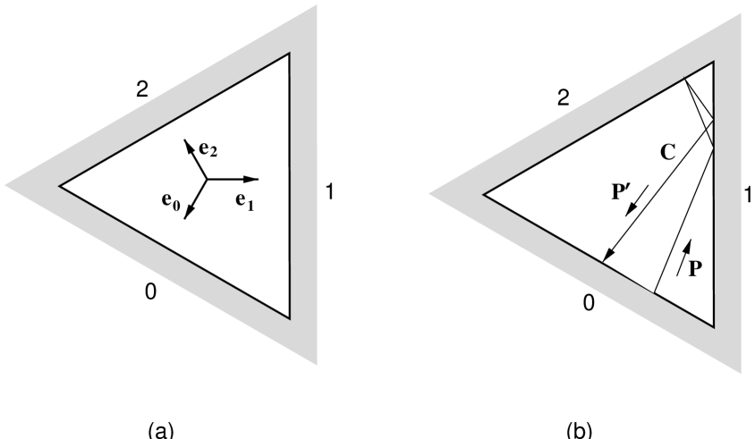
Figure 1: (a) Potential walls in $A_{2}$ affine Toda theory. (b) A wave with momentum ${\bf P}$ near the zeroth wall comes back to the same wall with momentum ${\bf P}^{\prime}$ after a series of reflections.

The quantization condition can be derived using the arguments of sect.3. For the moment we assume that the circumference of the cylinder is $2\pi$. Consider the path $C$ of a wave which starts with momentum ${\bf P}$ and comes back (after a series of reflections by other walls) to the zeroth potential wall with momentum ${\bf P}^{\prime}$. It will then be reflected by the zeroth wall. Fig.1(b) illustrates a multiple reflection in the two-dimensional potential. To satisfy the self-consistency condition, the momentum ${\bf P}^{\prime}$ after the last reflection by the zeroth wall should be equal to the incoming momentum ${\bf P}$ so that $\hat{s}_{0}{\bf P}^{\prime}={\bf P}$. Furthermore, since the zeroth wall is again Liouville-type, the momenta ${\bf P}^{\prime}=\hat{s}_{0}{\bf P}$ of the incident wave and ${\bf P}$ of the reflected wave should satisfy Eq.(41) which leads to

$$\frac{A(\hat{s}_{0}{\bf P})}{A({\bf P})}=S_{L}({\bf P}\cdot{\bf e}_{0}).$$ (44)

On the other hand, since $\hat{s}_{0}$ is given by a product of the Weyl reflections corresponding to simple roots, each representing the reflection experienced by the wave along the path $C$, the left hand side of Eq.(44) can be obtained from Eq.(43). Therefore, Eq.(44) gives a nontrivial quantization condition for the momentum ${\bf P}$. This condition can be generalized using the same arguments for other potential walls instead of the zeroth one. Then we obtain

$$\frac{A(\hat{s}_{0}\hat{s}{\bf P})}{A(\hat{s}{\bf P})}=S_{L}(\hat{s}{\bf P}\cdot{\bf e}_{0})\,.$$ (45)

where $\hat{s}$ is an arbitrary Weyl group element.

Using Eq.(43) we can write (45)

$$\left(\pi\mu\gamma(b^{2})\right)^{i{\bf P}\cdot\hat{s}{\bf v}/b}\left[\prod_{\boldsymbol{\alpha}>0}\frac{G(\hat{s}{\bf P}\cdot\hat{s}_{0}\boldsymbol{\alpha})}{G(\hat{s}{\bf P}\cdot\boldsymbol{\alpha})}\right]\frac{G(\hat{s}{\bf P}\cdot{\bf e}_{0})}{G(-\hat{s}{\bf P}\cdot{\bf e}_{0})}=1\,,$$ (46)

where

$${\bf v}=\hat{s}_{0}\boldsymbol{\rho}-\boldsymbol{\rho}+{\bf e}_{0}=-({\bf e}_{0}\cdot\boldsymbol{\rho}){\bf e}_{0}+{\bf e}_{0}=h{\bf e}_{0}$$

and we define a function

$$G(P)=\Gamma\left(1-iP/b\right)\Gamma\left(1-iPb\right).$$

The $\Gamma$-function factors in Eq.(46) can be further simplified. First, consider the action of $\hat{s}_{0}$ on a positive root $\boldsymbol{\alpha}$: $\hat{s}_{0}\boldsymbol{\alpha}=\boldsymbol{\alpha}-{\bf e}_{0}({\bf e}_{0}\cdot\boldsymbol{\alpha})$, which is either $\boldsymbol{\alpha}$ or $\boldsymbol{\alpha}+{\bf e}_{0}$ if $\boldsymbol{\alpha}\neq-{\bf e}_{0}$ since $-{\bf e}_{0}$ is the maximal root. In the first case, the factor $G(\hat{s}{\bf P}\cdot\hat{s}_{0}\boldsymbol{\alpha})$ in Eq.(46) is cancelled out by the same factor in the denominator, while, in the second case, there is no cancellation since $\boldsymbol{\alpha}+{\bf e}_{0}$ is a negative root. Finally, $\hat{s}_{0}{\bf e}_{0}=-{\bf e}_{0}$ and the corresponding factor $G(\hat{s}{\bf P}\cdot{\bf e}_{0})$ appears twice in Eq.(45). Using the property ${\bf e}_{0}\cdot\boldsymbol{\alpha}=0$ or $1$ for $\boldsymbol{\alpha}>0$ ($\boldsymbol{\alpha}\neq-{\bf e}_{0}$) and ${\bf e}_{0}\cdot{\bf e}_{0}=2$, we can simplify Eq.(46) as

$$\left(\pi\mu\gamma(b^{2})\right)^{ih{\bf P}\cdot\hat{s}{\bf e}_{0}/b}\prod_{\boldsymbol{\alpha}>0}\left[\frac{G(-{\bf P}\cdot\hat{s}\boldsymbol{\alpha})}{G({\bf P}\cdot\hat{s}\boldsymbol{\alpha})}\right]^{-\hat{s}\boldsymbol{\alpha}\cdot\hat{s}{\bf e}_{0}}=1\,.$$ (47)

Since the Weyl element $\hat{s}$ is arbitrary, Eq.(47) leads to the following condition for the lowest energy state

$$2hQL{\bf P}=2\pi\boldsymbol{\rho}-\sum_{\boldsymbol{\alpha}>0}\boldsymbol{\alpha}\delta(P_{\boldsymbol{\alpha}})\,,$$ (48)

where

$$L=-\frac{1}{2(1+b^{2})}\log[\pi\mu\gamma(b^{2})]\,,$$

and

$$\delta(P)=-i\log\frac{\Gamma(1+iP/b)\Gamma(1+iPb)}{\Gamma(1-iP/b)\Gamma(1-iPb)}\,.$$ (49)

This is the quantization condition for the momentum ${\bf P}$ in the $\mu\rightarrow 0$ limit. We see that effectively each positive root $\boldsymbol{\alpha}$ causes a phase shift of Liouville type.

Now we consider the system defined on a cylinder with the circumference $R$. When we scale back the size from $R$ to $2\pi$, the parameter $\mu$ in the action (1) changes to

$$\mu\rightarrow\mu\left(\frac{R}{2\pi}\right)^{2(1+b^{2})}.$$ (50)

The $\mu\rightarrow 0$ limit is realized as the deep UV limit $R\to 0$. The rescaling changes the definition of $L$ in Eq.(48) by

$$L=-\log\frac{R}{2\pi}-\frac{1}{2(1+b^{2})}\log[\pi\mu\gamma(b^{2})]\,.$$ (51)

The ground state energy with the circumference $R$ is given by

$$E(R)=-{\pi c_{\rm eff}\over{6R}}\quad{\rm with}\quad c_{\rm eff}=r-12{\bf P}^{2}$$ (52)

where ${\bf P}$ satisfies Eq.(48).

In this limit, Eq.(48) can be solved perturbatively. For this we expand the function $\delta(P)$ in Eq.(49) in powers of $P$,

$$\delta(P)=\delta_{1}(b)P+\delta_{3}(b)P^{3}+\delta_{5}(b)P^{5}\cdots\,,$$ (53)

where

$$\delta_{1}(b) = -2Q\gamma_{E}\,,$$

$$\delta_{3}(b) = \frac{2}{3}\zeta(3)(b^{3}+b^{-3})\,,$$

$$\delta_{5}(b) = -\frac{2}{5}\zeta(5)(b^{5}+b^{-5}).$$ (54)

Using the relation

$$\sum_{\boldsymbol{\alpha}>0}(\boldsymbol{\alpha})^{a}(\boldsymbol{\alpha})^{b}=h\delta^{ab},$$

we obtain

$$hl{\bf P}=2\pi\boldsymbol{\rho}-\delta_{3}(b)\sum_{\boldsymbol{\alpha}>0}\boldsymbol{\alpha}(P_{\boldsymbol{\alpha}})^{3}-\delta_{5}(b)\sum_{\boldsymbol{\alpha}>0}\boldsymbol{\alpha}(P_{\boldsymbol{\alpha}})^{5}-\cdots\,,$$

with

$$l\equiv 2QL+\delta_{1}\,.$$ (55)

The above equation can be solved iteratively in powers of $1/l$. Inserting the solution into Eq.(52), we find

$$c_{\rm eff}=r-\frac{r(h+1)}{h}\left[\left(\frac{2\pi}{l}\right)^{2}-\frac{24\delta_{3}}{2\pi}\left(\frac{2\pi}{l}\right)^{5}D_{4}(G)-\frac{24\delta_{5}}{2\pi}\left(\frac{2\pi}{l}\right)^{7}D_{6}(G)+{\cal O}(l^{-8})\right]$$ (56)

where the coefficients $D(G)$ are given in terms of a scalar product $\rho_{\boldsymbol{\alpha}}=\boldsymbol{\rho}\cdot\boldsymbol{\alpha}$ by

$$D_{4}(G)=\frac{1}{r(h+1)h^{4}}\sum_{\boldsymbol{\alpha}>0}\rho_{\boldsymbol{\alpha}}^{4}\,,\qquad D_{6}(G)=\frac{1}{r(h+1)h^{6}}\sum_{\boldsymbol{\alpha}>0}\rho_{\boldsymbol{\alpha}}^{6}\,.$$

The values of $D_{4}(G)$ and $D_{6}(G)$ can be evaluated explicitly:

$$D_{4}(A_{n-1})={(2n^{2}-3)\over 60n^{2}}\,,\qquad D_{6}(A_{n-1})={(n^{2}-2)(3n^{2}-5)\over 168n^{4}}\,,$$

$$D_{4}(D_{n})={(16n^{3}-45n^{2}+27n+8)\over 480(n-1)^{3}}\,,$$

$$D_{6}(D_{n})={(48n^{5}-213n^{4}+262n^{3}+6n^{2}-101n-32)\over 84(2(n-1))^{5}}\,,$$

$$D_{4}(E_{n})={r(h+1)\over 24(r+2)h}\,,\qquad(n=6,\ 7,\ 8)\,,$$

$$D_{6}(E_{6})={43\cdot 73\over 8\cdot(12)^{4}}\,,$$

$$D_{6}(E_{7})={514001\over 14\cdot(18)^{5}}\,,$$

$$D_{6}(E_{8})={(31)^{2}\over 54\cdot(30)^{2}}\,.$$ (57)

Using the relation (7) between the parameter $\mu$ in the action and the parameter ${\overline{m}}$ characterizing the spectrum, we can represent the effective central charge (56) for the simply-laced ATFTs in terms of dimensionless value ${\overline{m}}R$. In this form it can be compared with TBA results.

We note that expansion (56,57) for $D_{n}$ ATFTs can be continued to the half-integer $n$. The $D_{n}$ Toda theories with half-integer $n=l+1/2$ were studied in [19]. Besides the bosonic fields $\boldsymbol{\varphi}$ these models include the Majorana fermion $\psi$. The corresponding scattering theory is also self-dual ($b\to 1/b$). To obtain the values of $c_{\rm eff}(R)$ for these models we should express $c_{\rm eff}(R)$ in terms of parameter $mR$ where $m$ is defined by Eq.(2) and take the continuation for $r=n$, $h=2(n-1)$, and $k(D_{n})=2^{{n-3\over{2(n-1)}}}$ to the half-integer $n=l+1/2$. In particular, for $n=3/2$ we obtain exactly the expansion for the supersymmetric ShG model found in [7].

Example: $A_{2}$ ATFT

As a simplest example, we consider the $A_{2}$ ATFT more explicitly. In this case, there are two simple roots ${\bf e}_{1}$ and ${\bf e}_{2}$, and the affine root ${\bf e}_{0}$ is given by ${\bf e}_{0}=-({\bf e}_{1}+{\bf e}_{2})$. For each simple root, a Liouville-type potential wall is placed in the normal direction and the walls form a regular triangle as shown in Fig.1.

As the coefficient $\mu\to 0$, the size of the triangle becomes large and the zero-mode dynamics reduces to the quantum mechanical problem in two dimensions surrounded by a triangular potential wall where the potential vanishes except the vicinity of the walls. The energy eigenstate of the system is then the standing wave in the triangle which is a superposition of plane waves with momenta reflected by walls as explained in sect.3. Since the Weyl group ${\cal W}$ of $A_{2}$ algebra consists from six elements, ${\cal W}=\{1,\hat{s}_{1},\hat{s}_{2},\hat{s}_{1}\hat{s}_{2},\hat{s}_{2}\hat{s}_{1},\hat{s}_{1}\hat{s}_{2}\hat{s}_{1}=\hat{s}_{2}\hat{s}_{1}\hat{s}_{2}=\hat{s}_{0}\}$, the wave function can be written as a sum of six plane waves generated by the Weyl reflections as in Eq.(40) with their coefficients determined by Liouville reflection amplitudes. For example, if one considers the path $C$ of Fig.1 followed by a wave with momentum ${\bf P}$, one finds

$$A(\hat{s}_{1}{\bf P}) = S_{L}({\bf P}\cdot{\bf e}_{1})A({\bf P})\,,$$

$$A(\hat{s}_{2}\hat{s}_{1}{\bf P}) = S_{L}(\hat{s}_{1}{\bf P}\cdot{\bf e}_{2})A(\hat{s}_{1}{\bf P})=S_{L}(\hat{s}_{1}{\bf P}\cdot{\bf e}_{2})S_{L}({\bf P}\cdot{\bf e}_{1})A({\bf P})\,,$$

$$A(\hat{s}_{1}\hat{s}_{2}\hat{s}_{1}{\bf P}) = S_{L}(\hat{s}_{2}\hat{s}_{1}{\bf P}\cdot{\bf e}_{1})A(\hat{s}_{2}\hat{s}_{1}{\bf P})=S_{L}(\hat{s}_{2}\hat{s}_{1}{\bf P}\cdot{\bf e}_{1})S_{L}(\hat{s}_{1}{\bf P}\cdot{\bf e}_{2})S_{L}({\bf P}\cdot{\bf e}_{1})A({\bf P})\,,$$

which can be summarized as Eq.(43).

If the wave is further reflected by the zeroth wall, we have

$$A(\hat{s}_{0}\hat{s}_{1}\hat{s}_{2}\hat{s}_{1}{\bf P}) = S_{L}(\hat{s}_{1}\hat{s}_{2}\hat{s}_{1}{\bf P}\cdot{\bf e}_{0})A(\hat{s}_{1}\hat{s}_{2}\hat{s}_{1}{\bf P})$$ (58)

$$= S_{L}(\hat{s}_{1}\hat{s}_{2}\hat{s}_{1}{\bf P}\cdot{\bf e}_{0})S_{L}(\hat{s}_{2}\hat{s}_{1}{\bf P}\cdot{\bf e}_{1})S_{L}(\hat{s}_{1}{\bf P}\cdot{\bf e}_{2})S_{L}({\bf P}\cdot{\bf e}_{1})A({\bf P})\,.$$

Since $\hat{s}_{0}=\hat{s}_{1}\hat{s}_{2}\hat{s}_{1}$, Eq.(58) gives a quantization condition for ${\bf P}$ which is the special case of Eq.(46). Simplifying the arguments of $S_{L}$ in Eq.(58), we find

$$S_{L}({\bf P}\cdot{\bf e}_{1})S_{L}({\bf P}\cdot{\bf e}_{2})S_{L}({\bf P}\cdot({\bf e}_{1}+{\bf e}_{2}))^{2}=1\,,$$

which is equivalent to Eq.(47).

5 Comparison with the TBA results

A standard approach to study the scaling behaviour of integrable QFTs is to solve the TBA equations. In this section we compute the scaling functions of the ATFTs in the UV region from the TBA equations and compare them with the results in Eq.(56) based on the reflection amplitudes.

The TBA equations for the ATFTs are given by ($i=1,\cdots,r$)

$$m_{i}R\cosh\theta=\epsilon_{i}(\theta,R)+\sum_{j=1}^{r}\int\varphi_{ij}(\theta-\theta^{\prime})\log\left(1+e^{-\epsilon_{i}(\theta^{\prime})}\right){d\theta^{\prime}\over 2\pi},$$ (59)

where $\varphi_{ij}$ is the kernel which is equal to the logarithmic derivative of the $S$-matrix $S_{ij}(\theta)$ in Eq.(11)

$$\varphi_{ij}(\theta)=-i{d\over d\theta}\log S_{ij}(\theta)=\delta^{\prime}_{ij}(\theta).$$

These are $r$-coupled nonlinear integral equations for the ‘pseudo-energies’ $\epsilon_{i}(\theta,R)$ which give the scaling function of the effective central charge

$$c_{\rm eff}(R)=\sum_{i=1}^{r}\frac{3Rm_{i}}{\pi^{2}}\int\cosh\theta\log\left(1+e^{-\epsilon_{i}(\theta)}\right)d\theta.$$ (60)

It is quite difficult task to solve the TBA equations analytically and compare directly with Eq.(56). To obtain higher order terms in $1/l$ expansion, one needs to solve complicated coupled nonlinear differential equations. Even the lowest order terms at the order of $1/l^{2}$ contain constants which can not be decided by the scattering data. While the method used in [7] may be applicable here, we will concentrate only on numerical analysis of the TBA equations to avoid any digression to different problem.

Even the numerical analysis is limited if the rank $r$ grows since a large number of equations amplify the numerical errors entering in the iteration procedure. Therefore we will consider a few ATFTs with low ranks in each series of A-D-E, namely, $A_{2}$, $A_{3}$, $A_{4}$, $D_{4}$ and $E_{6}$ ATFTs. The effective central charge $c_{\rm eff}(R)$ is computed by solving Eq.(60) iteratively as a function of ${\overline{m}}R$. In order to compare the numerical data with our results based on the reflection amplitudes, we fit the numerical data for $c_{\rm eff}(R)$ from the TBA equations for many different values of $R$ with the function (56) where $\delta_{1}$, $\delta_{3}$ and $\delta_{5}$ are considered as the fitting parameters. For this comparison the relation (7) between the parameter $\mu$ in the action and parameter ${\overline{m}}$ for the particle masses is used. These parameters $\delta_{i}$’s are then compared with Eq.(4) defined from the reflection amplitude of the LFT. Since we already separate out the dependence on the Lie algebra $G$, our numerical results for the parameters $\delta_{i}$’s should be independent of $G$.

Tables 1–3 show the values of parameters $\delta_{i}$’s obtained numerically from TBA equations for different values of the coupling constant $B$ in $A_{2}$, $A_{3}$, $A_{4}$, $D_{4}$ and $E_{6}$ ATFTs. We see that they are in excellent agreement with those values of $\delta_{i}$’s following from the reflection amplitudes supplemented with Eq.(7). Thus numerical TBA analysis fully supports the validity of our whole scheme based on the reflection amplitude, $\mu$-${\overline{m}}$ relation and the quantization condition on ${\bf P}$.

B $\delta^{\rm(RA)}_{1}$ $\delta_{1}^{\rm(TBA)}(A_{2})$ $\delta_{1}^{\rm(TBA)}(A_{3})$ $\delta_{1}^{\rm(TBA)}(A_{4})$ $\delta_{1}^{\rm(TBA)}(D_{4})$ $\delta_{1}^{\rm(TBA)}(E_{6})$ 0.20 –2.88608 –2.88608 –2.884 0.25 –2.66604 –2.66604 –2.66603 –2.664 0.30 –2.51918 –2.51918 –2.51918 –2.51915 –2.5186 0.35 –2.42035 –2.42035 –2.42035 –2.42035 –2.42033 0.40 –2.35647 –2.35647 –2.35647 –2.35647 –2.35647 –2.3568 0.45 –2.32049 –2.32049 –2.32049 –2.32049 –2.32049 –2.3208 0.50 –2.30886 –2.30886 –2.30886 –2.30886 –2.30886 –2.30886

Table 1: $\delta_{1}^{\rm(RA)}$ vs. $\delta_{1}^{\rm(TBA)}$ for $A_{2},A_{3},A_{4},D_{4}$, and $E_{6}$ ATFTs.

B $\delta^{\rm(RA)}_{3}$ $\delta_{3}^{\rm(TBA)}(A_{2})$ $\delta_{3}^{\rm(TBA)}(A_{3})$ $\delta_{3}^{\rm(TBA)}(A_{4})$ $\delta_{3}^{\rm(TBA)}(D_{4})$ $\delta_{3}^{\rm(TBA)}(E_{6})$ 0.20 6.51114 6.509 0.25 4.31827 4.3180 4.310 0.30 3.08111 3.08100 3.08113 3.06 2.92 0.35 2.34480 2.34473 2.34484 2.3445 2.3438 0.40 1.90842 1.90839 1.90845 1.90845 1.90759 1.93 0.45 1.67590 1.67588 1.67592 1.67592 1.67589 1.69 0.50 1.60274 1.60273 1.60276 1.60276 1.60276 1.6028

Table 2: $\delta_{3}^{\rm(RA)}$ vs. $\delta_{3}^{\rm(TBA)}$ for $A_{2},A_{3},A_{4},D_{4}$, and $E_{6}$ ATFTs.

B $\delta^{\rm(RA)}_{5}$ $\delta_{5}^{\rm(TBA)}(A_{2})$ $\delta_{5}^{\rm(TBA)}(A_{3})$ $\delta_{5}^{\rm(TBA)}(A_{4})$ $\delta_{5}^{\rm(TBA)}(D_{4})$ $\delta_{5}^{\rm(TBA)}(E_{6})$ 0.20 –13.2856 –12.7 0.25 –6.49225 –6.38 0.30 –3.49933 –3.45 –3.55 –3.57 0.35 –2.03774 –2.01 –2.07 –1.97 –2.30 0.40 –1.29349 –1.281 –1.31 –1.31 –1.01 –2.5 0.45 –0.93614 –0.929 –0.95 –0.95 –0.94 –2.0 0.50 –0.82954 –0.823 –0.84 –0.84 –0.84 –0.87

Table 3: $\delta_{5}^{\rm(RA)}$ vs. $\delta_{5}^{\rm(TBA)}$ for $A_{2},A_{3},A_{4},D_{4}$, and $E_{6}$ ATFTs.

The agreement is relatively poor for $\delta_{5}$ for the cases with high rank such as $E_{6}$ partly due to the numerical errors in higher order calculations. Another reason comes from the fact that neglected terms in the $1/l$ expansion (the order of ${\cal O}(1/l^{8})$ or higher) in Eq.(56) may not be sufficiently small compared with terms with $\delta_{5}$. However, one can in principle reduce these errors by increasing the accuracy of the numerical calculations. There are also corrections of ${\cal O}(R^{\gamma})$ to the expansion of $c_{\rm eff}(R)$ in power series of $1/l$ which increase as $B$ goes to zero. This explains why the discrepancies in the tables increase as $B$ decreases.

In Fig.2, we also plot the scaling functions $c_{\rm eff}(R)$ as a function of $R$ setting ${\overline{m}}=1/2$ for different ATFTs; first, using numerical solutions of the TBA equations and, second, using Eqs.(48) and (52) based on the reflection amplitudes. To compare the same objects, we added to the second case the contribution from the bulk vacuum energy term [20, 12]

$$\Delta c_{\rm eff}={3{\overline{m}}^{2}R^{2}\over{2\pi}}{\sin(\pi/h)\over{\sin(\pi B/h)\sin(\pi(1-B)/h)}}$$ (61)

which becomes significant for $R\geq 0.01$. For each model, the two curves are almost identical without any noticeable difference in the graphs even upto $R\sim{\cal O}(1)$.

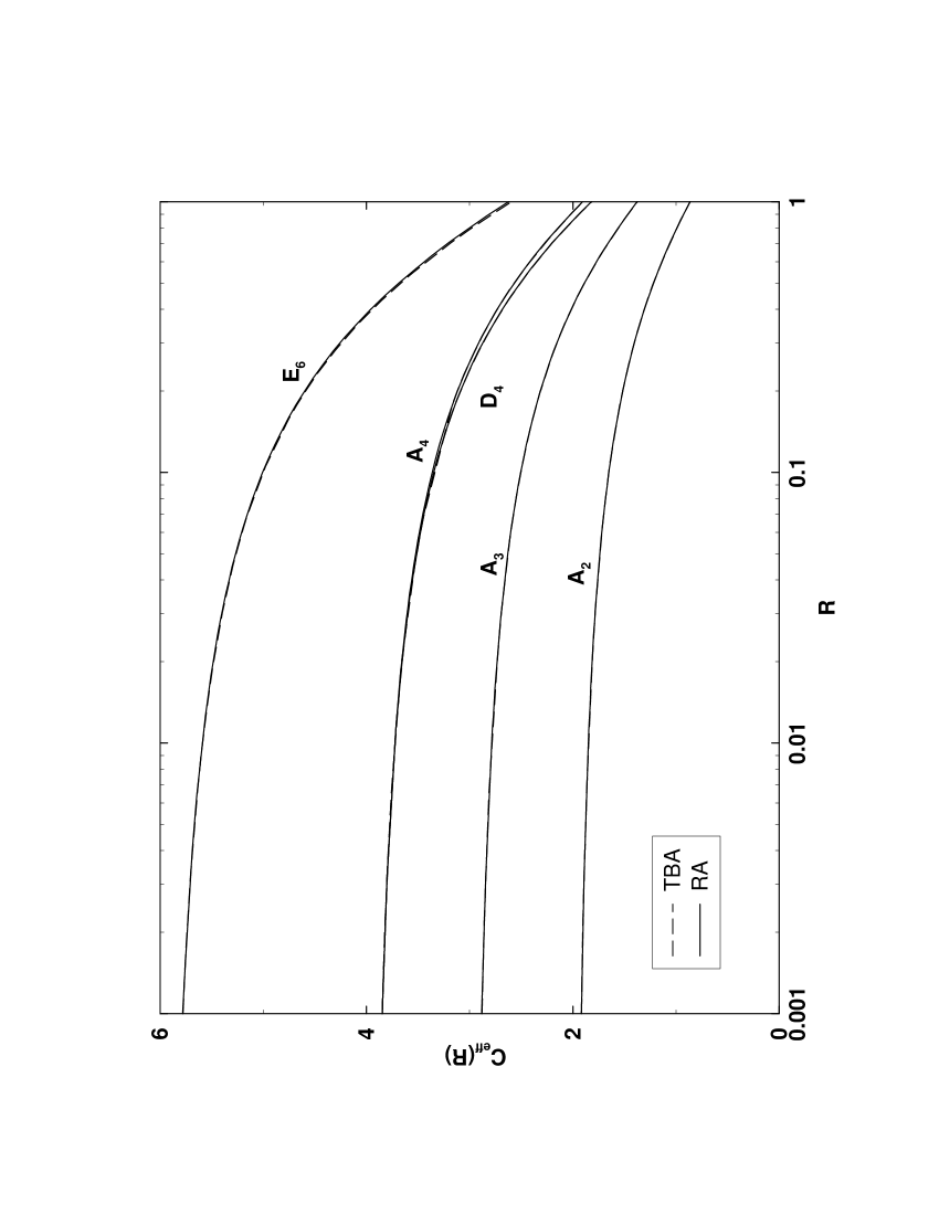
Figure 2: Plot of $c_{\rm eff}$ for $A_{2},A_{3},A_{4},D_{4},A_{6}$, and $E_{6}$ ATFTs at $B=0.5$.

6 Concluding remarks

In the main part of this paper we considered the UV asymptotics of the ground state energy in ATFTs. The main objects which were used for this analysis were the reflection amplitudes (28) of NATTs. As it was mentioned in sect. 2 these objects also play a crucial role in the calculation of the one poin functions in perturbed CFT. The one point functions of the exponential fields

$$\mathcal{G}(\boldsymbol{a})=\langle\exp\boldsymbol{a}\cdot\boldsymbol{\varphi}\rangle$$

in ATFTs can be reconstructed from the reflection amplitudes (28). It followes from the results of the paper [17] that these functions satisfy to the functonal equations similar to the relations (19, 30). For the ADE series of ATFTs these functions were calculated in [23] and have the form:

$$\mathcal{G}(\boldsymbol{a})=\left(\frac{\bar{m}k(G)\Gamma\left(\frac{1}{(1+b^{2})h}\right)\Gamma\left(1+\frac{b^{2}}{h(1+b^{2})}\right)}{2\Gamma(1/h)}\right)^{-a^{2}}\exp{\mathcal{T}}(\boldsymbol{a})$$

here

$$\mathcal{T}(\boldsymbol{a})=\int\frac{dt}{t}\left[\psi(t)\,\sum_{\alpha>0}\sinh(ba_{\boldsymbol{\alpha}}t)\,\sinh\left((b(a-2Q)_{\boldsymbol{\alpha}}+h(1+b^{2}))t\right)+e^{-2t}a^{2}\right]$$

where $k(G)$. $a_{\boldsymbol{\alpha}}$, $Q_{\boldsymbol{\alpha}}$ are defined by Eqs. (8), (27) and

$$\psi(t)=-\frac{\sinh((1+b^{2})t)}{\sinh t\sinh(b^{2}t)\,\sinh((1+b^{2})ht)}$$

We suppose to discuss the application of these functions to the analysis of ATFTs and related perturbed CFT in another publication.

In the previous sections we studied the UV asymptotics for the simply laced ATFTs. It looks interesting to extend this consideration to the case of dual pairs of non simply lased ATFTs. To do this it is necessary to generalize the quantization condition (48) and the relations (7) between the parameters of the action and masses of the particles. The work in this direction is in progress.

Appendix: $A_{n-1}$ Quantum Toda Chain

In this Appendix we obtain the quantization conditions for one-dimensional $A_{n-1}$ quantum Toda chain using the approach based on the integrability of this theory. The quantum Toda chain corresponds to the semiclassical ($b\to 0$) approach to the zero-mode dynamics of the ATFT, however, the structure of quantization condition for this system is similar to Eq.(48).

The quantum Toda chain is described by the Hamiltonian

$$H={1\over{2}}\sum_{i=1}^{n}p_{i}^{2}+\kappa^{2}\sum_{i=1}^{n}e^{b(q_{i}-q_{i+1})}$$ (62)

where $q_{n+1}\equiv q_{1}$. The model (62) is integrable. The diagonalization of the Hamiltonian was done in a remarkable paper by Sklyanin [21] who used the quantum inverse scattering method to obtain the Bethe ansatz (BA) equations for the eigenvalues of $H$. Here we show that for $\kappa<<1$ these BA equations can be represented in the form similar to Eq.(48).

The Lax operator for Toda chain (62) has the form

$$L_{i}(u)=\left(\begin{array}[]{cc}u-p_{i}&-\kappa e^{bq_{i}}\\ \kappa e^{-bq_{i}}&0\end{array}\right).$$ (63)

The commuting family of the transfer matrices $T(u)$ corresponding to the Lax operator Eq.(63) can be written as:

$$T(u)={\rm Tr}\left(L_{1}(u)\ldots L_{n}(u)\right),\qquad\left[T(u),T(u^{\prime})\right]=0.$$ (64)

The operators $T(u)$ is a polynomial of degree $n$ with the coefficients:

$$T(u)=u^{n}+T_{1}u^{n-1}+T_{2}u^{n-2}+\ldots$$ (65)

where $T_{1}=-\sum_{i=1}^{n}p_{i}=P$ and $T_{2}=-H+P^{2}/2$. The BA equations for the eigenvalues $t(u)$ of the operator $T(u)$ can be formulated in terms of eigenvalues $Q(u)$ of Baxter’s $Q$-operator [22]. Namely, these equations have the form [21]

$$t(u)Q(u)=\kappa^{n}\left(i^{n}Q(u+ib)+i^{-n}Q(u-ib)\right)$$ (66)

where $t(u)$ is a polynomial of $u$, which can be written as

$$t(u)=\prod_{i=1}^{n}(u-v_{i}),\quad{\rm with}\quad P=\sum_{i=1}^{n}v_{i},\quad E=\sum_{i=1}^{n}v_{i}^{2}/2,$$ (67)

and $Q(u)$ is an entire function of $u$.

With these two conditions Eq.(66) is rather complicated to be solved analytically. Even for $n=2$ it can be only reduced to the Mathieu equation. Here we consider the approximate solution of Eq.(66) with accuracy ${\cal O}(\kappa^{n})$. Namely, we impose the condition that function $Q(u)$ is a meromorphic function with the absolute values of residues at the poles ${\cal O}(\kappa^{n})$.

The function $Q(u)$ with this analyticity property which satisfies to Eq.(66) with accuracy ${\cal O}(\kappa^{n})$ can be written in the form

$$Q(u)=\exp\left({iun\log\kappa\over{b}}\right)\prod_{i=1}^{n}\Gamma\left({i(v_{i}-u)\over{b}}\right)+\exp\left(-{iun\log\kappa\over{b}}\right)\prod_{i=1}^{n}\Gamma\left({i(u-v_{i})\over{b}}\right).$$ (68)

The function $Q(u)$ has the poles at real $u=v_{i}$ with the residues ${\cal O}(1)$ and the poles in the complex plane with the residues ${\cal O}(\kappa^{n})$. To satisfy the analyticity condition we should cancel the poles at $u=v_{j}$. In this way we arrive at the following equations for parameters $v_{j}$:

$$\exp\left({2inv_{j}\log\kappa\over{b}}\right)\prod_{i\neq j}{\Gamma\left(1+{i(v_{i}-v_{j})\over{b}}\right)\over{\Gamma\left(1-{i(v_{i}-v_{j})\over{b}}\right)}}=(-1)^{n-1}$$ (69)

or taking the logarithm on both sides:

$$-{2nv_{j}\log\kappa\over{b}}={1\over{i}}\sum_{i\neq j}\log{\Gamma\left(1+{i(v_{i}-v_{j})\over{b}}\right)\over{\Gamma\left(1-{i(v_{i}-v_{j})\over{b}}\right)}}+\pi I_{j}$$ (70)

where $I_{j}$ is the set of different integers, odd (even) for even (odd) $n$.

The minimal set of numbers $I_{j}$ corresponding to the ground state with center of mass momentum $P=0$ can be written as:

$$I_{j}=2j-n-1,\quad j=1,\ldots,n.$$ (71)

One can easily see that with this set of numbers $I_{j}$ Eq.(70) is similar to Eq.(48) which has additional term $\Delta\varphi(v_{j})$ in the RHS:

$$\Delta\varphi(v_{j})=\sum_{i\neq j}{1\over{i}}\log{\Gamma\left(1+i(v_{i}-v_{j})b\right)\over{\Gamma\left(1-i(v_{i}-v_{j})b\right)}}$$

coming from the quantum renormalization of reflection amplitudes in the two-dimensional NATT.

References

• [1] A. B. Zamolodchikov, Int. J. Mod. Phys. A4 (1989) 4235.
• [2] C. N. Yang and C. P. Yang, J. Math. Phys., 10 (1969) 1115.
• [3] Al. B. Zamolodchikov, Nucl. Phys. B342 (1990) 695.
• [4] Al. B. Zamolodchikov, β€œResonance factorized scattering and roaming trajectories”, prepreint ENS-LPS-335 (1991).
• [5] V. A. Fateev, E. Onofri, and Al. B. Zamolodchikov, Nucl. Phys. B406 (1993) 521.
• [6] A. B. Zamolodchikov and Al. B. Zamolodchikov, Nucl. Phys. B477 (1996) 577.
• [7] C. Ahn, C. Kim, and C. Rim, Nucl. Phys. B556 (1999) 505.
• [8] M. J. Martins, Nucl. Phys. B394 (1993) 339.
• [9] A. Fring, C. Korff and B. J. Schulz, Nucl. Phys. B549 (1999) 579.
• [10] M. A. Olshanetsky and A. M. Perelomov, Phys. Rep. 94 (1983) 313.
• [11] Al. B. Zamolodchikov, Int. J. Mod. Phys. A10 (1995) 1125.
• [12] V. A. Fateev, Phys. Lett. B324 (1994) 45.
• [13] A. Arinstein, V. Fateev, and A. Zamolodchikov, Phys. Lett. B87 (1979) 389.
• [14] H. W. Braden, E. Corrigan, P. E. Dorey, and R. Sasaki, Nucl. Phys. B338 (1990) 689.
• [15] T. Oota, Nucl. Phys. B504 (1997) 738.
• [16] V. Fateev and S. Lukyanov, Sov. Sci. Rev. A212 (Physics) (1990) 212.
• [17] V. Fateev, S. Lukyanov, A. Zamolodchikov, and Al. Zamolodchikov, Phys. Lett. B406 (1997) 83.
• [18] J. E. Humphreys, β€œIntroductions to Lie Algebras and Representation Theory”, Springer Verlag (1972).
• [19] G. W. Delius, M. T. Grisaru, S. Penati, and D. Zanon, Phys. Lett. B256 (1991) 164; C. Destri, H. de Vega, and V. Fateev, Phys. Lett. B256 (1991) 173.
• [20] C. Destri and H. de Vega, Nucl. Phys. B358 (1991) 251.
• [21] E. K. Sklyanin, β€œThe Quantum Toda Chain”, Preprint LPTHE Paris 84-34 (1984); Lect. Notes in Phys. 226 (1985) 196.
• [22] R. J. Baxter, Ann. Phys. 70 (1972) 193.
• [23] V.Β Fateev, β€œNormalization factors in CFT and their applications” preprint LPM-11 (1999).