Dynamical Chiral Symmetry Breaking on the Light Front  I. DLCQ Approach

Abstract

Dynamical chiral symmetry breaking in the DLCQ method is investigated in detail using a chiral Yukawa model closely related to the Nambu-Jona-Lasinio model. By classically solving three constraints characteristic of the light-front formalism, we show that the chiral transformation defined on the light front is equivalent to the usual one when bare mass is absent. A quantum analysis demonstrates that a nonperturbative mean-field solution to the “zero-mode constraint” for a scalar boson $\sigma$ can develop a nonzero condensate $\langle\sigma\rangle=-\frac{\lambda}{N}\langle\bar{\Psi}\Psi\rangle\neq 0$ while a perturbative solution cannot. This description is due to our identification of the “zero-mode constraint” with the gap equation. The mean-field calculation clarifies unusual chiral transformation properties of fermionic field, which resolves a seemingly inconsistency between triviality of the null-plane chiral charge $Q_{5}^{\rm LF}|0\rangle=0$ and nonzero condensate $\langle\bar{\Psi}\Psi\rangle\neq 0$. We also calculate masses of scalar and pseudoscalar bosons for both symmetric and broken phases, and eventually derive the PCAC relation and nonconservation of $Q_{5}^{\rm LF}$ in the broken phase.

I Introduction

Chiral symmetry breaking is undoubtedly one of the most important concepts for understanding hadron physics in low energy region [1]. The smallness of $\pi$ and $K$ masses is beautifully explained if one identifies them with the Nambu-Goldstone (NG) bosons associated with the chiral symmetry breaking. An important aspect of this phenomenon is dynamical formation of NG bosons as bound states of quarks and gluons in the strong coupling region. However, its complete demonstration in QCD is not reached yet because of the difficulties in describing bound states in a nonperturbative and relativistic manner. Instead, many people have been investigating much simpler effective models of QCD. Among them, the Nambu-Jona-Lasinio (NJL) model [2] is the most deeply and thoroughly understood. The NJL model is a 3+1 dimensional four-Fermi theory and reproduces various properties of hadrons concerning the chiral symmetry breaking despite some undesirable features such as nonrenormalizability and lack of confinement [3]. Nowadays the model plays a role of laboratory in which we can test new ideas proposed for nonperturbative study of low energy QCD. Therefore the NJL model is the most appropriate model in which we can check whether the light-front (LF) quantization can be applied to the dynamical chiral symmetry breaking. The LF quantization is a newly revamped nonperturbative method for solving relativistic bound states in quantum field theory [4].

Let us explain why the chiral symmetry breaking becomes a special issue in the LF formalism. The reason is twofold: the first is apparent contradiction between a nontrivial vacuum and a LF “trivial” vacuum, and the second is peculiarity of LF chiral transformation. To resolve these problems is our primary purpose in the present paper. One of the remarkable merits of the LF quantization is that the Fock vacuum defined by a free theory is also the vacuum of the full theory. Many technical advantages such as exact Fock state expansion arise from this fact. On the contrary, the conventional formulation says that the chiral symmetry breaking is essentially a physics of finding another vacuum that breaks the chiral symmetry but is energetically favored. Such “vacuum physics” is thought to be very important for understanding nonperturbative phenomena in low energy region. Therefore to apply the LF formalism to QCD necessarily entails a problem how to realize such “vacuum physics” within a framework with a trivial vacuum. For the purpose of understanding this problem, there are considerable efforts [5] to describe the spontaneous symmetry breaking in a simple scalar model ($\lambda\phi_{1+1}^{4}$). They succeeded in obtaining the critical coupling which is consistent with the conventional results. The key is to solve a constraint equation for the longitudinal zero mode (“zero-mode constraint”) which appears in the DLCQ (Discretized Light-Cone Quantization) method [6]. A nonzero condensate is realized as a nonperturbative solution of the zero-mode constraint. We will discuss this method in more detail later.

Compared with such extensive studies, only little is known about the dynamical symmetry breaking in fermionic systems. Especially there have been only few attempts about the NJL model on the LF [7, 8, 9, 10]. At first glance, it seems not possible to follow the same route as in the scalar models because we do not have bosonic fields as fundamental degrees of freedom in the NJL model. However, we can apply the same idea to the dynamical symmetry breaking if one introduces bosonic auxiliary fields to the fermion bilinears and raises them to dynamical variables by adding their kinetic terms. Of course the original fermionic model is reproduced as an infinitely heavy mass limit of the bosonic fields. According to this idea, we succeeded in describing the dynamical symmetry breaking (discrete chiral symmetry) in the 1+1 dimensional four-Fermi theory (the Gross-Neveu model) [11]. The present paper is a generalization of this preliminary work which discussed only discrete chiral symmetry. We consider a kind of Yukawa model with continuous chiral symmetry, which is obtained from the NJL model using the above technique. We work within the DLCQ method so that we can formulate the problem from the viewpoint of the zero-mode constraints. It should be commented however that it is possible to discuss the dynamical symmetry breaking even without introducing auxiliary fields. In Ref. [8], one of the authors insisted the importance of a “fermionic constraint” which is again unique to the LF formulation and has very complicated structure due to the four-Fermi interaction. (Another merit of including scalar fields is a quite simplification of the fermionic constraint.) More detailed analysis in this direction will be reported in the next paper [12].

One more point to be discussed is the unusual behavior of chiral transformation on the LF. In the LF formulation, a half degree of freedom of the fermion is a dependent variable to be represented by other independent variables. Therefore, chiral transformation should be imposed only on the independent component of the fermion [13]. It is not clear in interacting models whether the LF chiral transformation is equivalent to the usual one or not.

The paper is organized as follows. In the next section, we define the chiral Yukawa model which is closely related to the NJL model and introduce our framework, the DLCQ method. The classical aspects of the model is discussed in Sec. III. Here, we see that there are three constraints (i.e. two zero-mode constraints and one fermionic constraint). We also show peculiarity of the LF chiral transformation and explicitly give the null-plane chiral charge $Q_{5}^{\rm LF}$. Quantum analysis, which is the main part of this paper, is developed in Sections IV and V. In Sec. IV, we demonstrate that perturbative and nonperturbative treatments of the solution to the constraints give different description of the model. In Sec. V, we discuss some physics consequences of the nonperturbative analysis. Especially, we resolve a problem of contradiction between the triviality of the null-plane charge and the nonzero condensate. We further calculate the masses of scalars in the symmetric and broken phases. Then we discuss the PCAC relations and nonconservation of the LF chiral charge $Q_{5}^{\rm LF}$ in the broken phase. The last section is devoted to conclusion and discussions.

II The model

Here we introduce the model (chiral Yukawa model) and summarize the standard knowledge on the chiral symmetry breaking in the conventional equal-time formulation. We also define our setup of the problem following the DLCQ method.

A Definition of the model

The NJL model was first introduced as the simplest $3+1$ dimensional example which exhibits the dynamical chiral symmetry breaking [2]. In its original form there were two flavors, but a one flavor model

$${\cal L_{\rm NJL}}=\bar{\Psi}^{a}(i\hbox to0.0pt{/\hss}\partial-m)\Psi^{a}+\frac{\lambda}{2N}\left[\left(\bar{\Psi}^{a}\Psi^{a}\right)^{2}+\left(\bar{\Psi}^{a}i\gamma_{5}\Psi^{a}\right)^{2}\right]$$

also breaks the chiral symmetry which exists in the massless case $m=0$. We give an additional internal structure to the fermion independently of the flavor, and treat an $N$-component spinor $\Psi^{a}$ in order to clarify the validity of approximation we use. From now on, summation over $a=1,\ldots,N$ is always implied. Since this model is not renormalizable, we must specify a regularization scheme such as a cutoff to uniquely determine the model and to obtain finite results.

In this paper, we discuss more general model with Yukawa interactions:

$${\cal L} = \bar{\Psi}^{a}(i\hbox to0.0pt{/\hss}\partial-m)\Psi^{a}+{N\over 2\mu^{2}}(\partial_{\mu}\sigma\partial^{\mu}\sigma+\partial_{\mu}\pi\partial^{\mu}\pi)$$ (2)

$$-{N\over 2\lambda}(\sigma^{2}+\pi^{2})-(\sigma\bar{\Psi}^{a}\Psi^{a}+\pi\bar{\Psi}^{a}i\gamma_{5}\Psi^{a}),$$

where $\sigma$ ($\pi$) is a scalar (pseudoscalar) boson with mass $\mu/\sqrt{\lambda}$ and $\mu$ is a dimensionless parameter. If one takes infinitely heavy mass limit for scalars $\mu\rightarrow\infty$, the dynamical scalars become auxiliary fields $\sigma=-\frac{\lambda}{N}\bar{\Psi}\Psi$, $\pi=-\frac{\lambda}{N}\bar{\Psi}i\gamma_{5}\Psi$ and the model goes back to the NJL model.

In order to contrast with our LF calculation, let us briefly comment on the usual story of chiral symmetry breaking in the NJL model [2]. When $m=0$, both of the lagrangian densities are invariant under the chiral transformation:

$$\Psi^{a} \rightarrow {\rm e}^{i\gamma_{5}\theta}\Psi^{a},$$ (3)

$$\left(\matrix{\sigma\cr\pi}\right) \rightarrow \left(\matrix{\cos 2\theta&\sin 2\theta\cr-\sin 2\theta&\cos 2\theta}\right)\left(\matrix{\sigma\cr\pi}\right)\equiv R(2\theta)\left(\matrix{\sigma\cr\pi}\right).$$ (4)

It should be reminded that this transformation is, of course, imposed on all the fields, which is, however, not the case in the LF formalism. This point will be discussed later in more detail. The usual story is as follows: The chiral symmetry breaks down spontaneously in a quantum level due to nonzero fermion condensate $\langle\bar{\Psi}\Psi\rangle\neq 0$. The most straightforward demonstration will be the mean field approximation with the concept of self-consistency. If one has $N$-component fermion, we can justify the mean field approximation by the leading approximation of $1/N$ expansion. The self-consistency condition is a crucial key to the description of broken phase. This condition directly leads to the gap equation which determines the value of condensate and, equivalently, the physical fermion mass. As a result of symmetry breaking, there emerges a Nambu-Goldstone boson. Since we do not have any fundamental scalar boson in the NJL model, the NG boson (pion) should be supplied dynamically as a bound state of a fermion and an anti-fermion. Mass of the pionic state indeed vanishes in the chiral limit.

It will be helpful to comment on the physics meaning of treating the model (2). First of all, we should clearly distinguish our model from the linear $\sigma$ model of Gell-Mann and Lévy [14]. Structurally our model resembles the $\sigma$ model in the sense that it consists of bosons and fermions interacting with each other via Yukawa couplings and has a continuous chiral symmetry. However, an important difference in our model is the absence of potential term for scalars. In the linear $\sigma$ model, it is the wine-bottle potential that induces the chiral symmetry breaking. Therefore the symmetry breaking occurs in the tree level and the dynamical formation of NG boson can not be seen. What we obtain is only the sigma condensate $\langle\sigma\rangle\neq 0$. This naturally leads us to identify the fermions with nucleons. On the other hand, the fermions in our model should be regarded as quarks rather than nucleons. Indeed, as far as the leading order of $1/N$ expansion is concerned, the model shows the same behavior as the NJL model. For example, straightforward calculations such as effective potential [16] or mean-field approximation show that the chiral symmetry breaking $\langle\sigma\rangle=-\frac{\lambda}{N}\langle\bar{\Psi}\Psi\rangle\neq 0$ occurs in the one-loop quantum level (see Appendix A for more details). Therefore we do not consider our model as a special case of the linear $\sigma$ model and in order to remind this, we call it the “chiral Yukawa model”.

It is also very important to view the NJL model as a low-energy effective theory of the chiral Yukawa model. The relation between two models is very similar to that between the Weinberg-Salam model and the Fermi theory of weak interaction: The chiral Yukawa model is renormalizable and the fermions interact with each other by exchanging scalar or pseudo-scalar bosons. If we take the infinitely heavy mass limit for bosons $\mu/\sqrt{\lambda}\rightarrow\infty$, then the theory reduces to the NJL model with non-renormalizable four-Fermi interactions. In this sense, the NJL model can be considered as a low energy effective theory of the chiral Yukawa model. Such low energy approximation will be valid when the momentum is much smaller than the mass of the exchanged particles $p^{2}\ll\mu^{2}/\lambda$. In this paper, we mainly treat the chiral Yukawa model for technical reasons, but what we eventually want to know are results of the NJL model. Therefore even if we encounter divergences during calculation in the chiral Yukawa model, we only regularize them by some cutoff scheme and do not renormalize them.

Finally, as far as we are discussing such ’low energy region’, we do not have to worry about the problem of double counting of physics degrees of freedom. In the NJL model, the scalar and pseudo-scalar bosons are described as quark-antiquark bound states. On the other hand, we treat the scalars as physically independent degrees of freedom in the chiral Yukawa model. So if we regard the fermions and scalars as quarks and mesons, there is the problem of double counting with which we are always confronted in treating chiral-quark type models [17]. However, in the low energy region, or equivalently for sufficiently large boson mass $\mu\rightarrow\infty$, the scalars become “frozen” and do not behave as propagating degrees of freedom.

B Setup in the LF quantization

We analyze the chiral Yukawa model (2) in the DLCQ method and take special care of the longitudinal zero modes of scalars. In this method, we compactify the longitudinal space into a circle $x^{-}\in[-L,L]$ with appropriate boundary conditions on fields. For scalars, we impose periodic boundary conditions at each LF time

$$\sigma(x^{-}=-L,~{}x_{\perp}) = \sigma(x^{-}=L,~{}x_{\perp}),$$ (5)

$$\pi(x^{-}=-L,~{}x_{\perp}) = \pi(x^{-}=L,~{}x_{\perp}),$$ (6)

so that we can explicitly treat the longitudinal zero modes defined by

$$\sigma_{0}(x_{\perp})=\frac{1}{2L}\int_{-L}^{L}dx^{-}\ \sigma(x),$$ (7)

$$\pi_{0}(x_{\perp})=\frac{1}{2L}\int_{-L}^{L}dx^{-}\ \pi(x).$$ (8)

Then the scalar fields are decomposed into the zero modes and the remaining oscillation modes:

$$\sigma(x)=\sigma_{0}(x_{\perp})+\varphi_{\sigma}(x),$$ (9)

$$\pi(x)=\pi_{0}(x_{\perp})+\varphi_{\pi}(x).$$ (10)

On the other hand, we impose an antiperiodic boundary condition for the fermion field,

$$\Psi^{a}(x^{-}=-L,~{}x_{\perp})=-\Psi^{a}(x^{-}=L,~{}x_{\perp}).$$ (11)

Here we must be careful about the boundary condition on the “bad component” of the fermion. As we discuss in the next section, if we decompose the fermion as

$$\Psi^{a}=\psi^{a}_{+}+\psi^{a}_{-},\quad\psi^{a}_{\pm}\equiv\Lambda_{\pm}\Psi^{a},$$ (12)

we find that $\psi_{-}$ (“bad component”) is a dependent field (see Appendix for the definition of $\Lambda_{\pm}$). So the boundary condition on $\psi_{-}$ should be imposed consistently with the dynamics. For example, if we imposed the periodic boundary condition on $\psi_{-}$ and antiperiodic on $\psi_{+}$, the mass term $\bar{\Psi}\Psi$ and the fermion’s kinetic term became antiperiodic. This is not desirable as a term in the lagrangian and even not consistent with the scalar sector. Then how about the periodic boundary conditions for both of $\psi_{+}$ and $\psi_{-}$? In this case we have a dynamical zero mode of $\psi_{+}$, which is, however, not important to our problem because the chiral condensate will be related to the zero modes of $\sigma$ or $\bar{\Psi}\Psi$. Periodic fermion will give unnecessary intricacy to the problem. Therefore the antiperiodic boundary condition (11) is appropriate.

III Classical aspect

Classical analysis is necessary for specifying independent degrees of freedom. In this section, we determine the constraint structure of the model and define the LF chiral transformation. Chiral current and charge are explicitly given.

A Constraints

The system has three important constraints characteristic of the LF formalism: a constraint for $\psi_{-}$ (fermionic constraint) and two constraints for zero modes of bosons (zero-mode constraints). The Euler-Lagrange equation for $\psi_{-}$ itself is the fermionic constraint:

$$i\partial_{-}\psi^{a}_{-}={1\over 2}(i\gamma^{\perp}\partial_{\perp}+m+\sigma-i\pi\gamma_{5})\gamma^{+}\psi^{a}_{+}~{}.$$ (1)

Also the zero-mode constraints for $\sigma_{0}(x_{\perp})$ and $\pi_{0}(x_{\perp})$ are easily obtained from $x^{-}$-integration of the Euler-Lagrange equations for $\sigma$ and $\pi$, respectively:

$$\left(\frac{\mu^{2}}{\lambda}-\partial_{\bot}^{2}\right)\left(\matrix{\sigma_{0}\cr\pi_{0}}\right)+\frac{\mu^{2}}{N}\left[\bar{\Psi}^{a}(x)\left(\matrix{1\cr i\gamma_{5}}\right)\Psi^{a}(x)\right]_{0}=0,$$

where $[\quad]_{0}$ denotes integration over $x^{-}$ (see Appendix B). More explicitly,

$$0=\left(\frac{\mu^{2}}{\lambda}-\partial_{\bot}^{2}\right)\left(\matrix{\sigma_{0}\cr\pi_{0}}\right)$$ (2)

$$-\frac{\mu^{2}}{N}\frac{1}{\sqrt{2}}\left[\psi_{+}^{a{\dagger}}\left(\matrix{-1\cr i\gamma_{5}}\right)\gamma^{-}\psi^{a}_{-}+\psi_{-}^{a{\dagger}}\left(\matrix{-1\cr i\gamma_{5}}\right)\gamma^{+}\psi^{a}_{+}\right]_{0}.$$ (3)

These equations mean that $\sigma_{0}$ and $\pi_{0}$ should be represented by other independent variables. If we take the $\mu\rightarrow\infty$ limit, the zero-mode constraints are reduced to zero-mode projected equations of the familiar relations $\sigma=-\frac{\lambda}{N}\bar{\Psi}\Psi$ and $\pi=-\frac{\lambda}{N}\bar{\Psi}i\gamma_{5}\Psi$. Eventually the independent degrees of freedom are nonzero modes of the scalars $\varphi_{\sigma},\ \varphi_{\pi}$, and the “good component” of the spinor $\psi_{+}$. The above constraints are, of course, derived from Dirac’s procedure (see Appendix C). It is easily found that they belong to the second class.

B Chiral transformation on the LF

Definition of chiral transformation on the LF is different from the usual one Eqs. (3) and (4). This is because the identification of independent degrees of freedom is not the same as usual. As we saw, $\sigma_{0},\pi_{0}$ and $\psi^{a}_{-}$ are dependent variables and should change as a result of transformation of the independent variables $\varphi_{\sigma},\varphi_{\pi}$ and $\psi^{a}_{+}$. Therefore in the LF formulation, we impose the chiral transformation only on the dynamical variables:

$$\psi_{+}^{a}\rightarrow{\rm e}^{i\theta\gamma_{5}}\psi_{+}^{a}~{},$$ (4)

$$\left(\matrix{\varphi_{\sigma}\cr\varphi_{\pi}}\right)\rightarrow R(2\theta)\left(\matrix{\varphi_{\sigma}\cr\varphi_{\pi}}\right),$$ (5)

where $R(2\theta)$ represents a rotation matrix defined in Eq. (4). These are the definition of the “LF chiral transformation”. If we find that $\psi_{-}$ and $(\sigma_{0},\pi_{0})$ also transform as $\psi_{-}\rightarrow{\rm e}^{i\theta\gamma_{5}}\psi_{-}$ and $\left(\matrix{\sigma_{0}\cr\pi_{0}}\right)\rightarrow R(2\theta)\left(\matrix{\sigma_{0}\cr\pi_{0}}\right)$ as a result of (4) and (5), we can say that the “LF chiral transformation” is substantially equivalent to the usual one (3) and (4). However, what is surprising about the “LF chiral transformation” is that the transformation (4) is an exact symmetry even for massive fermion as far as interaction is absent [13]. So it will be interesting to check whether the “LF chiral transformation” in our model is exact or not when a mass term is present.

In order to see the transformation property of the dependent variables, let us solve the constraints classically. This means that we completely ignore the ordering of the variables which becomes a burdensome but important issue in a quantum treatment. The fermionic constraint (1) which was originally a complicated relation in the purely fermionic NJL model, is now easily solved owing to introduction of scalars. The zero-mode constraints are also solved formally. Explicit form of the solutions is given in Appendix C. Now we find the transformation of the zero modes and subsequently that of $\psi_{-}$.

1 Massless fermion

Let us first consider the massless fermion case. When $m=0$, it is easy to see that the transformation (4) and (5) induces the following:

$$\left(\matrix{\sigma_{0}\cr\pi_{0}}\right)\rightarrow R(2\theta)\left(\matrix{\sigma_{0}\cr\pi_{0}}\right),$$ (6)

$$\psi^{a}_{-}\rightarrow{\rm e}^{i\theta\gamma_{5}}\psi^{a}_{-}.$$ (7)

This is identical with the usual chiral transformation. Therefore it is shown that when $m=0$ the fields do transform as (3) and (4) even on the LF at the classical level.

Now that we know all the transformation laws, it is straightforward to construct the Noether current and charge. The lagrangian with $m=0$ is invariant under the LF chiral transformations. Form of the LF chiral current is equivalent to the usual one,

$$j_{\mu}^{5}=-\bar{\Psi}{}^{a}\gamma_{\mu}\gamma_{5}\Psi^{a}+{2N\over\mu^{2}}\Big{(}\pi\partial_{\mu}\sigma-\sigma\partial_{\mu}\pi\Big{)}.$$ (8)

However, $\sigma_{0},\ \pi_{0}$ and $\psi_{-}$ in (8) should be understood as solutions of the constraints. On the other hand, the LF chiral charge $Q_{5}^{\rm LF}=\int_{-L}^{L}dx^{-}\int d^{2}x_{\perp}\ j^{+}_{5}$ does not include the constrained variables:

$$Q_{5}^{\rm LF}\!\!=\!\!\int\!\!d^{3}x\!\left[-\sqrt{2}\psi_{+}^{a{\dagger}}\gamma_{5}\psi^{a}_{+}+{2N\over\mu^{2}}\Big{(}\varphi_{\pi}\partial_{-}\varphi_{\sigma}-\varphi_{\sigma}\partial_{-}\varphi_{\pi}\Big{)}\right],$$ (9)

which is consistent with the fact that $Q_{5}^{\rm LF}$ is a generator of the chiral rotation for independent variables. Transformation of other dependent fields should be obtained through the change of dynamical variables.

2 Massive fermion

The massive fermion case is much more complicated. As mentioned before, an astonishing fact of the “LF chiral transformation” is that it is an exact symmetry even for a massive free fermion [13]. When the mass term is present, the “bad component” of free fermion does not transform as Eq. (7). Subsequently, the associated Noether current $\hat{J}_{\mu}^{5}$ has an extra term proportional to the bare mass

$$\widehat{J}_{\mu}^{5}=J_{\mu}^{5}-im(\bar{\psi}_{+}+\bar{\psi}_{-})\gamma_{\mu}\gamma_{5}\frac{1}{\partial_{-}}\gamma^{+}\psi_{+}.$$ (10)

Nevertheless, the divergence of the current turns out to be zero $\partial^{\mu}\widehat{J}_{\mu}^{5}=0$ due to the cancellation between the first term ($\partial^{\mu}J_{\mu}^{5}=-2im\bar{\Psi}\gamma_{5}\Psi$) and the second term. This should be compared with the usual current in the equal-time quantization: ${\cal J}_{\mu}^{5}=-\bar{\Psi}\gamma_{\mu}\gamma_{5}\Psi,\ \partial^{\mu}{\cal J}_{\mu}^{5}=-2im\bar{\Psi}\gamma_{5}\Psi$, which also holds for interacting theories and is intimately connected with PCAC relation. Note that the LF chiral charge $\widehat{Q}_{5}^{\rm LF}=\int d^{3}x\widehat{J}^{+}_{5}$ is equivalent to that in the massless case due to $\widehat{J}^{+}_{5}=J^{+}_{5}$. This is natural because the LF chiral transformation is defined irrespective of the mass term.

Now, how about the chiral Yukawa model? Using the solution for $m\neq 0$ (see Appendix C), the infinitesimal chiral transformation of $\sigma_{0}$, $\pi_{0}$ and $\psi_{-}$ are given as follows:

$$\left(\matrix{\delta\sigma_{0}\cr\delta\pi_{0}}\right)=\left(\matrix{2\theta\pi_{0}\cr-2\theta\sigma_{0}}\right)+\left(\matrix{0\cr 2\theta m\zeta}\right),$$ (11)

$$\delta\psi^{a}_{-}={i\theta\gamma_{5}}\psi^{a}_{-}-2i\theta\gamma_{5}m(1+\zeta)\frac{1}{2}\frac{1}{i\partial_{-}}\gamma^{+}\psi_{+}\>,$$ (12)

where

$$\zeta\equiv-{1\over\sqrt{2}}{\mu^{2}\over N}{\cal D}^{-1}(x_{\perp})\left[\psi_{+}^{a{\dagger}}\frac{1}{i\partial_{-}}\psi^{a}_{+}+\ {\rm c.c.}\ \right]_{0},$$

and ${\cal D}(x_{\perp})$ is the transverse differential operator defined in Appendix C. It is evident that the dependent fields do not transform as Eqs. (6) and (7). As a result, the Noether current (8) also gets modified by the term proportional to $m$. The explicit form of the current $\widehat{j}^{\mu}_{5}$ is very complicated but we can see that the $+$ component is equivalent to that of (8). Therefore the LF chiral charge is given by Eq. (9) even for massive case. However, contrary to the massive free fermion, the divergence of the LF current $\partial^{\mu}\widehat{j}_{\mu}^{5}$ does not vanish due to nontrivial interactions.

One of the lessons suggested by these observations is that when we investigate physics related to massive fermions (e.g. PCAC relation), we had better treat the current $j_{\mu}^{5}$ defined by the massless fermions rather than $\widehat{j}_{\mu}^{5}$. This is clear for the free case: The true LF chiral current $\widehat{J}_{\mu}^{5}$ (10) defined for the massive fermion vanishes if we take the divergence while that for massless fermion $J_{\mu}^{5}$ gives the usual relation. This is true of the chiral Yukawa model. The divergence of the current (8) is given as

$$\partial^{\mu}j_{\mu}^{5}=-2m\bar{\Psi}i\gamma_{5}\Psi$$ (13)

while $\partial^{\mu}\widehat{j}_{\mu}^{5}$ is very complicated. It will be very difficult to discuss the PCAC relations etc. by using $\widehat{j}_{\mu}^{5}$. It is not quite clear if analysis of $\widehat{j}_{\mu}^{5}$ makes sense. Instead, even for the massive case, we treat the current (8) to discuss the physics such as PCAC. This point will be discussed later again in Section V.

IV Quantum aspects

In the classical analysis, we formally solved the constraints in order to find the LF chiral current and charge. When $m=0$, the resulting hamiltonian is chiral symmetric and we do not have any symmetry breaking term. Therefore even if we go to quantum theory with such hamiltonian, we will not be able to describe the chiral symmetry breaking. Certainly it might be possible that we could find a broken phase hamiltonian by adjusting the operator ordering, but such procedure seems unnatural and tricky. Instead, we quantize the model before solving the constraints. This means that we perform the Dirac quantization for constrained systems. After that, the constraints are solved quantum mechanically with a care of the operator ordering. The same route has been traced by many people who tried to describe the spontaneous symmetry breaking of simple scalar systems [5].

Calculation of the Dirac brackets in our system is a very complicated task. However, the Dirac brackets between dynamical variables turn out to be standard ones: Quantization conditions for the dynamical variables $\varphi_{\sigma},\varphi_{\pi},$ and $\psi^{a}_{+}$ are

$$\Big{[}\varphi_{\xi}(x),~{}\varphi_{\eta}(y)\Big{]}_{x^{+}=y^{+}}$$ (1)

$$\quad=-\delta_{\xi\eta}\frac{\mu^{2}}{N}\frac{i}{4}\left(\epsilon(x^{-}-y^{-})-\frac{x^{-}-y^{-}}{L}\right)\delta^{(2)}(x_{\bot}-y_{\bot}),$$ (2)

$$\left\{\psi_{+\alpha}^{a}(x),\psi_{+\beta}^{b{\dagger}}(y)\right\}_{x^{+}=y^{+}}$$ (3)

$$\quad=\frac{1}{\sqrt{2}}(\Lambda_{+})_{\alpha\beta}\delta^{ab}\delta(x^{-}-y^{-})\delta^{(2)}(x_{\bot}-y_{\bot}),$$ (4)

where $\xi$ and $\eta$ stand for $\sigma$ or $\pi$, and $\alpha,\beta=1,\cdots,4$ are the spinor indices. The sign function $\epsilon(x^{-})$ is defined in Appendix B. The other commutators between dynamical variables are zero. Note that these conditions are irrespective of the phase of the model because they are independent of the interaction.

Mode expansion of the fields at $x^{+}=0$ reads

$$\varphi_{\eta}({\bf x})=\sqrt{\frac{\mu^{2}}{N}}\frac{1}{2L}\sum_{n=1,2\cdots}\frac{1}{2p_{n}^{+}}\int\frac{d^{2}p_{\perp}}{(2\pi)^{2}}$$ (5)

$$\hskip 28.45274pt\times\left\{a_{\eta}(p_{n}^{+},{\bf p}_{\perp})\ {\rm e}^{-i{\bf px}}+a_{\eta}^{{\dagger}}(p_{n}^{+},{\bf p}_{\perp})\ {\rm e}^{i{\bf px}}\right\},$$ (6)

$$\psi_{+}^{a}({\bf x})=\frac{1}{2L}\sum_{n=\frac{1}{2},\frac{3}{2}\cdots}\int\frac{d^{2}p_{\perp}}{\sqrt{2\pi}2^{3/4}\sqrt{p_{n}^{+}}}$$ (7)

$$\hskip 56.9055pt\times\sum_{h=\pm\frac{1}{2}}\left\{w(h)b^{a}(p_{n}^{+},{\bf p}_{\perp},h)\ {\rm e}^{-i{\bf px}}\right.$$ (8)

$$\hskip 85.35826pt+\left.w(-h)d^{a{\dagger}}(p_{n}^{+},{\bf p}_{\perp},h)\ {\rm e}^{i{\bf px}}\right\},$$ (9)

where ${\bf px}=p_{n}^{+}x^{-}-{\bf p}_{\perp}{\bf x}_{\perp}$ and $p_{n}^{+}=\pi n/L$. The spinors $w(\pm h)$ depend only on the helicity $h$ [13]. It follows that

$$\left[a_{\xi}(p_{n}^{+},{\bf p}_{\perp}),\ a^{\dagger}_{\eta}(q_{m}^{+},{\bf q}_{\perp})\right]$$ (10)

$$\hskip 85.35826pt=(2\pi)^{2}(2L)2p_{n}^{+}\delta_{nm}\delta({\bf p}_{\perp}-{\bf q}_{\perp})\delta_{\xi\eta},$$ (11)

$$\left\{b^{a}(p_{n}^{+},{\bf p}_{\perp},h),\ b^{b{\dagger}}(q_{m}^{+},{\bf q}_{\perp},h^{\prime})\right\}$$ (12)

$$\hskip 85.35826pt=2p_{n}^{+}\frac{2L}{2\pi}\delta_{nm}\delta({\bf p}_{\perp}-{\bf q}_{\perp})\delta_{hh^{\prime}},$$ (13)

$$\left\{d^{a}(p_{n}^{+},{\bf p}_{\perp},h),\ d^{b{\dagger}}(q_{m}^{+},{\bf q}_{\perp},h^{\prime})\right\}$$ (14)

$$\hskip 85.35826pt=2p_{n}^{+}\frac{2L}{2\pi}\delta_{nm}\delta({\bf p}_{\perp}-{\bf q}_{\perp})\delta_{hh^{\prime}}.$$ (15)

It is important to note that both of the above mode expansions are independent of the mass. (The spinors $w(\pm h)$ are independent of mass. This is clearly shown in the Appendix of Ref. [9].) This means that if we calculate $n$-point Green functions at fixed time $x^{+}=0$, they will become independent of the value of mass, which is not a correct result in general. This undesirable situation is known as one of the pathological properties of the LF formalism which needs great care for obtaining correct results [18]. Indeed, as we will see later, to remedy this problem is indispensable to get a meaningful gap equation. In many cases, loss of mass information is cured by a carefully chosen infrared regularization. It should also be commented that the mass-information loss is certainly not a desirable feature, but we will find its usefulness in describing the broken phase physics. Anyway, we must pay great attention to the fact that naive mode expansion of the (scalar and fermion) fields is independent of the value of mass.

The Fock vacuum $|0\rangle$ is defined by

$$a_{\sigma}(p_{n}^{+},{\bf p}_{\perp})|0\rangle=a_{\pi}(p_{n}^{+},{\bf p}_{\perp})|0\rangle$$ (16)

$$\quad=b^{a}(p_{n}^{+},{\bf p}_{\perp},h)|0\rangle=d^{a}(p_{n}^{+},{\bf p}_{\perp},h)|0\rangle=0,$$ (17)

for $n>0$. It is worth while emphasizing that the vacuum of this system is really the Fock vacuum since we have no dynamical zero modes. Because of the $p^{+}$ conservation, the normal-ordered chiral charge $Q_{5}^{\rm LF}$ always annihilates the vacuum:

$$Q_{5}^{\rm LF}|0\rangle=0.$$ (18)

It has been known that any light-like charge $Q^{\rm LF}$ automatically leaves the vacuum invariant $Q^{\rm LF}|0\rangle=0$ whether or not it generates a symmetry [19].

In a quantum theory, operator ordering becomes an issue. Let us comment on the problem of operator ordering and clarify our stance toward it. Since the (zero-mode and fermionic) constraint equations are generally nonlinear relations among operators, their solutions depend on operator ordering. We must select an appropriate operator ordering. Then, what can be the criterion for this problem? In many papers discussing the spontaneous symmetry breaking in DLCQ, the Weyl ordering is adopted on general grounds. However, it is not clear whether the Weyl ordering in constraint equations makes sense because they include both independent and dependent variables. The most reliable criterion for determining the operator ordering will be as follows. Before solving the constraint equations, we can calculate the Dirac brackets between independent variables and dependent ones (e.g. $[\sigma_{0},\psi_{+}]=\cdots$), which are terribly complicated in our model and we do not display them in this paper. Here we already have to specify the operator ordering. On the other hand, we can solve the constraint relations with the above ordering and obtain their solutions such as $\sigma_{0}=\sigma_{0}(\varphi_{\sigma},\varphi_{\pi},\psi_{+})$. Now we can calculate again the commutators between the solutions (i.e. dependent variables) and independent variables (e.g. $[\sigma_{0}(\varphi_{\sigma},\varphi_{\pi},\psi_{+}),\psi_{+}]$ ) using simple commutators Eqs. (1) and (4). The results should be identical with those of the Dirac bracket. In other words, we must find out such operator ordering that will give a consistent result in the above sense. This should be the criterion for an appropriate operator ordering. However, as you expect, to find such ordering in our model is an extremely difficult task. So practically, we just work with several particular orderings and compare the results. In our actual calculations, we treat two specific orderings and check whether the results depend on the ordering or not. To find a consistent operator ordering should be examined in much simpler models.

In the following, we will solve the zero-mode constraints in two different ways: perturbative and non-perturbative methods. To solve the constraint is significant to describe the symmetry breaking on the LF. To see this, let us decompose the longitudinal zero modes into c-number parts and normal-ordered operator parts,

$$\sigma_{0}=\sigma_{0}^{({\rm c})}+\sigma_{0}^{({\rm op})},$$ (19)

$$\pi_{0}=\pi_{0}^{({\rm c})}+\pi_{0}^{({\rm op})}.$$ (20)

If the c-number part of the solution is nonvanishing, it directly means nonzero condensate: $\langle 0|\sigma|0\rangle=\sigma_{0}^{({\rm c})}\neq 0$ and $\langle 0|\pi|0\rangle=\pi_{0}^{({\rm c})}\neq 0$. Therefore to find such nontrivial solution is necessary to describe the symmetry breaking. We explicitly demonstrate that perturbative solutions cannot lead to chiral symmetry breaking while nonperturbative solutions give nonzero vacuum expectation value for $\sigma$. In both cases, the fermionic constraint is formally solved (as in Eq. (C7)) and inserted into the zero-mode constraints.

A Perturbative solutions to the zero-mode constraints

Let us solve the zero-mode constraints using perturbation in terms of the coupling constant $\lambda$. Since $\lambda$ is a dimensionful parameter, we introduce some scale $\lambda_{\rm cr}$ which is much larger than $\lambda$ ($\lambda_{\rm cr}\gg\lambda$). We regard $\lambda_{\rm cr}$ as a critical coupling of the symmetry breaking which will be determined later. Now we expand the constrained variables as follows

$$\sigma_{0}=\sum_{n=0}^{\infty}\left(\frac{\lambda}{\lambda_{\rm cr}}\right)^{n}\sigma_{0}^{(n)},$$ (21)

$$\pi_{0}=\sum_{n=0}^{\infty}\left(\frac{\lambda}{\lambda_{\rm cr}}\right)^{n}\pi_{0}^{(n)},$$ (22)

$$\psi^{a}_{-}=\sum_{n=0}^{\infty}\left(\frac{\lambda}{\lambda_{\rm cr}}\right)^{n}\psi_{-}^{a(n)},$$ (23)

and the dynamical variables are treated as $O((\frac{\lambda}{\lambda_{\rm cr}})^{0})$. Inserting the above expansions into the constraints Eqs. (1) and (3) with the natural ordering and comparing the same order of perturbation, we obtain the solution order by order. For example, the lowest order solutions are

$$\sigma_{0}^{(0)}=\pi_{0}^{(0)}=0,$$ (24)

$$\psi_{-}^{a(0)}={1\over 2}{1\over i\partial_{-}}(i\gamma^{\perp}\partial_{\perp}+m+\varphi_{\sigma}-i\varphi_{\pi}\gamma_{5})\gamma^{+}\psi^{a}_{+}.$$ (25)

Higher order solutions are given in Appendix D.

The chiral transformation of the perturbative solution in the massless case can be inductively checked. First, it is easy to see that the 0-th and 1st order solutions rotate symmetrically under the LF chiral transformation (4) and (5). If we suppose the $n$-th order solutions rotate chirally, the $n+1$-th order solutions also behave the same. Eventually the perturbative solution transforms symmetrically under the LF chiral rotation (4) and (5),

$$\left[Q_{5}^{\rm LF},\Psi^{a}\right]=\gamma_{5}\Psi^{a}~{},$$ (26)

$$\left[Q_{5}^{\rm LF},\sigma\right]=-2i\pi~{},\qquad\left[Q_{5}^{\rm LF},\pi\right]=2i\sigma~{}.$$ (27)

Of course the hamiltonian [cf) Eq. (C6)] is also invariant $[Q_{5}^{\rm LF},\ H]=0$ which is the same as the classical analysis in the previous section.

What is most important is that the vacuum expectation values of the perturbative solutions vanish in all order of perturbation $\langle 0|\sigma_{0}|0\rangle=\langle 0|\pi_{0}|0\rangle=0$. This is easily verified by using $\langle 0|\varphi_{\sigma,\pi}|0\rangle=0$ and $\langle 0|\psi_{+}^{\dagger}\partial_{\perp}\psi_{+}|0\rangle=0$. Therefore we are in a chiral symmetric phase:

$$\langle 0|\sigma|0\rangle=\langle 0|\pi|0\rangle=0.$$ (28)

B Nonperturbative solutions to the zero-mode constraints

We next solve the zero-mode constraints using the mean-field approximation. In the following, we work with a particular operator ordering though the result is the same as others as far as we discuss the leading order of $1/N$ expansion. The following ordering greatly reduces our calculation. Substituting the solution of the fermionic constraint into the zero-mode constraints and rearrange the ordering, we obtain

$$0 = \Big{(}{\mu^{2}\over\lambda}-\partial_{\perp}^{2}\Big{)}\left(\matrix{\sigma_{0}\cr\pi_{0}}\right)$$ (29)

$$+ {1\over 2^{3/2}}{\mu^{2}\over N}{1\over 2L}\int_{-L}^{L}\!\!dx^{-}\int_{-L}^{L}\!\!dy^{-}\frac{\epsilon(x^{-}-y^{-})}{2i}$$ (30)

$$\times \left\{i\psi_{+}^{a{\dagger}}(x)\left(\matrix{-1\cr i\gamma_{5}}\right)\gamma^{\perp}\partial_{\perp}\psi^{a}_{+}(y)\right.$$ (32)

$$\quad-i\partial_{\perp}\psi_{+}^{a{\dagger}}(y)\left(\matrix{-1\cr i\gamma_{5}}\right)\gamma^{\perp}\psi^{a}_{+}(x)$$

$$+ \left(\matrix{m+\sigma(y)\cr\pi(y)}\right)\left(\psi_{+}^{a{\dagger}}(x)\psi^{a}_{+}(y)-\psi_{+}^{a{\dagger}}(y)\psi^{a}_{+}(x)\right)$$ (33)

$$- \left.\left(\matrix{-\pi(y)\cr m+\sigma(y)}\right)\left(\psi_{+}^{a{\dagger}}(x)i\gamma_{5}\psi^{a}_{+}(y)+\psi_{+}^{a{\dagger}}(y)i\gamma_{5}\psi^{a}_{+}(x)\right)\right\}$$ (35)

$$+\ {\rm h.c.},$$

where $\psi^{a}_{+}(y)=\psi^{a}_{+}(x^{+},y^{-},x_{\perp})$ and similarly for $\sigma(y)$ and $\pi(y)$ The operator ordering here is different from that in the perturbative treatment. However, one can show that the previous perturbative result does not change with the above ordering. That is, the perturbative solution with the above ordering does not lead to chiral symmetry breaking.

Let us first determine the c-number part of the zero modes defined by Eqs. (19) and (20). We saw in the classical analysis that $(\sigma_{0},\pi_{0})$ rotates chirally in the massless case. Therefore we choose

$$\sigma_{0}^{({\rm c})}\neq 0,$$ (36)

$$\pi_{0}^{({\rm c})}=0.$$ (37)

Taking a vacuum expectation value of the zero-mode constraint for $\sigma$ greatly simplifies the calculation, which is an advantage of our specific choice of ordering:

$$\frac{\mu^{2}}{\lambda}\sigma_{0}^{(\rm c)} \!\!\!\!=-\frac{1}{\sqrt{2}}\frac{\mu^{2}}{N}(m+\sigma_{0}^{(\rm c)})$$ (38)

$$\times \left\langle 0\left|\left[\psi_{+}^{a{\dagger}}\frac{1}{i\partial_{-}}\psi^{a}_{+}-\left(\frac{1}{i\partial_{-}}\psi_{+}^{a{\dagger}}\right)\psi^{a}_{+}\right]_{0}\right|0\right\rangle.$$ (39)

Introducing $M$ defined by

$$M\equiv m+\sigma_{0}^{(\rm c)}~{},$$ (40)

and evaluating the vacuum expectation value in Eq. (39) by using the mode expansion, we have

$$M - m$$ (41)

$$= -\frac{1}{\sqrt{2}}\frac{\lambda}{N}M\left\langle 0\left|\left[\psi_{+}^{a{\dagger}}\frac{1}{i\partial_{-}}\psi^{a}_{+}-\left(\frac{1}{i\partial_{-}}\psi_{+}^{a{\dagger}}\right)\psi^{a}_{+}\right]_{0}\right|0\right\rangle$$ (42)

$$= \lambda M{2\over(2\pi)^{3}}\int d^{2}p_{\bot}\sum_{n=1/2,\cdots}{\Delta p^{+}\over p_{n}^{+}},$$ (43)

where $\Delta p^{+}=\pi/L$. The operator form of the right-hand-side suggests us to identify as

$$\frac{M}{\sqrt{2}}\left\langle 0\left|\left[\psi_{+}^{a{\dagger}}\frac{1}{i\partial_{-}}\psi^{a}_{+}-\left(\frac{1}{i\partial_{-}}\psi_{+}^{a{\dagger}}\right)\psi^{a}_{+}\right]_{0}\right|0\right\rangle$$ (44)

$$=\left\langle 0\left|\left[\bar{\Psi}_{M}^{a}\Psi_{M}^{a}\right]_{0}\right|0\right\rangle,$$ (45)

where $\Psi_{M}^{a}$ is a fermion with mass $M$,

$$\Psi^{a}_{M} = \psi^{a}_{+}+\psi^{a}_{-M}~{},$$ (46)

$$\psi^{a}_{-M} \equiv {1\over 2}{1\over i\partial_{-}}(i\gamma^{\perp}\partial_{\perp}+M)\gamma^{+}\psi^{a}_{+}~{}.$$ (47)

($\psi^{a}_{-M}$ is the “bad” component of $\Psi^{a}_{M}$.) Therefore it is natural to consider $M$ to be the physical fermion mass. In other words, the identification in Eq. (45) corresponds to the self-consistency condition.

Eq. (43) should be the gap equation by which we can determine $\sigma_{0}^{(c)}$ and equivalently, the physical fermion mass $M$. However, it is not evident to regard it as the gap equation because Eq. (43) in the chiral limit $m\rightarrow 0$ cannot give nonzero $M$. The same situation was observed in our previous work on the Gross-Neveu model [11]. As was discussed in Ref. [11], if we want a meaningful gap equation, we must supply mass information so that Eq. (43) possesses a nontrivial solution $M\neq 0$ in the chiral limit when we regularize the divergent summation over $n$. The need of the mass dependence in Eq. (43) is readily understood from the identification in Eq. (45). Indeed, one can easily check that $\langle 0|\bar{\Psi}_{M}\Psi_{M}|0\rangle/M$ should explicitly depend on $M$ in the equal-time formulation. This is a typical example of the “mass-information loss” on the LF [18] which must be repaired properly for obtaining correct results.

It may be possible to regularize the divergent summation in Eq. (43) with, say, a heat-kernel damping factor [11], but such calculation is complicated and not tractable. Instead, we introduce some cutoff that renders the divergent summation into finite one. Such cutoff should be introduced so that the result correctly depends on the mass $M$. Here for simplicity, we adopt a cutoff which eventually reduces to the parity invariant (PI) cutoff $p^{\pm}<\Lambda$ [8]. From the dispersion relation and the PI cutoff, we find that the momentum region is restricted to $(M^{2}+{\bf p}_{\bot}^{2})/2\Lambda<p_{n}^{+}=\pi n/L<\Lambda$. Therefore we set

$$n_{\rm IR}<n<n_{\rm UV},$$ (48)

where $n_{\rm IR}$ and $n_{\rm UV}$ are nearest half-integers to $\frac{L}{\pi}\frac{M^{2}+{\bf p}_{\bot}^{2}}{2\Lambda}$ and $\frac{L}{\pi}\Lambda$ respectively. If we use the approximation for a large half-integer $\widetilde{n}$, $\sum_{n=1/2,\cdots}^{\widetilde{n}}n^{-1}\simeq{\rm ln}{\widetilde{n}}+{\rm ln}4e^{\gamma}$, the summation is approximated as

$$\sum_{n=1/2,\cdots}{\Delta p^{+}\over p_{n}^{+}}=\sum_{n=n_{\rm IR}+1}^{n_{\rm UV}-1}\frac{1}{n}\simeq{\rm ln}\frac{n_{\rm UV}}{n_{\rm IR}}\simeq{\rm ln}\frac{2\Lambda^{2}}{M^{2}+{\bf p}_{\bot}^{2}},$$ (49)

for fixed $\Lambda$, $M$ and ${\bf p}_{\bot}^{2}$ and sufficiently large $L$. Of course there is “finite volume effect” for finite $L$, but we finally take the infinite volume limit and the finite volume effect is expected to be small as far as $L$ is large enough. Eventually Eq. (43) becomes dependent on the mass $M$ and can be considered to be a gap equation

$$M-m=\lambda M\frac{\Lambda^{2}}{4\pi^{2}}\left\{2-\frac{M^{2}}{\Lambda^{2}}\left(1+{\rm ln}\frac{2\Lambda^{2}}{M^{2}}\right)\right\}.$$ (50)

Form of this gap equation is different from those with familiar cutoff schemes such as the three or four momentum cutoff [3], but our gap equation behaves exactly the same as usual. Indeed, even in the chiral limit $m\rightarrow 0$, this equation is a nonlinear equation for $M$ and when the coupling constant $\lambda$ is larger than the critical value $\lambda_{\rm cr}=2\pi^{2}/\Lambda^{2}$, there is a nontrivial solution $M=M_{0}\neq 0$ (see FIG. 1). This also means that the zero mode of $\sigma$ has been determined as $\sigma_{0}^{({\rm c})}=M-m$. Furthermore, one should note that the gap equation (50) is independent of the value of $\mu$. So we can regard the finite $\mu$ result $\langle\sigma\rangle=M-m$ as the result for infinite $\mu$; $-\frac{\lambda}{N}\langle\bar{\Psi}\Psi\rangle=M-m$. (Remember that the $\mu\rightarrow\infty$ limit of (3) is $\sigma_{0}=-\frac{\lambda}{N}[\bar{\Psi}\Psi]_{0}$.) Therefore the chiral symmetry breaking occurs for arbitrary value of $\mu$ in the mean-field approximation. This is consistent with the result of the conventional equal-time quantization (see Appendix A).

On the other hand, there is a trivial solution $M=0$ (when $m=0$) even for $\lambda>\lambda_{\rm cr}$ and if we select this solution the resulting theory becomes chiral symmetric. Then there comes a problem which solution should be physically realized. Unfortunately, comparison of the vacuum energy for both phases does not tell anything about this problem because the vacuum energies turn out to be the same. If we found the consistent operator ordering as discussed before, we could estimate difference of the vacuum energies and determine the physically realized phase. Even without such calculation, however, we can say that the symmetric solution is excluded for $\lambda>\lambda_{\rm cr}$. This is because there emerge tachyonic modes and the system becomes unstable if we select a trivial solution for $\lambda>\lambda_{\rm cr}$. This will be again discussed in Section V-B. So we deal with only the nontrivial solution for $\lambda>\lambda_{\rm cr}$ and do not consider the symmetric solution.

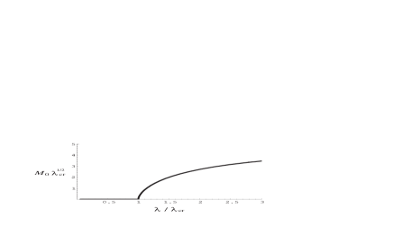
FIG. 1.: Fermion’s dynamical mass $M_{0}$ in the chiral limit as the solution of the gap equation (50). There is a nonzero solution for $\lambda>\lambda_{\rm cr}$.

Comments on other cutoff schemes are in order. We find a nontrivial equation for $M$ by using the PI cutoff. It was crucial to include the mass information as the regularization. However, we have to be careful in setting the cutoff. Any cutoff scheme which holds mass does not necessarily lead to a physically sensible result [21]. For example, a two dimensional PI cutoff $M^{2}/2\Lambda<p^{+}<\Lambda$ with a transverse cutoff $|{\bf p}_{\perp}|<\Lambda$ gives a wrong result. The resulting gap equation erroneously predicts that there is no symmetric phase. It seems important to introduce a cutoff with some symmetry considerations. Indeed, the three momentum cutoff respecting the three dimensional rotation [7] and the PI cutoff [8] in our case predict the existence of the critical coupling constant.

Now let us determine the operator parts of the zero modes by the mean-field approximation. We approximate the nonlinear terms in Eq. (35) by using $AB\approx A\langle B\rangle+\langle A\rangle B-\langle A\rangle\langle B\rangle$, where the expectation values are taken with respect to the Fock vacuum. We further neglect contribution from the oscillating modes of scalars $\varphi_{\sigma}=\varphi_{\pi}=0$. Then the operator parts are given by

$$\left(\matrix{\sigma^{(\rm op)}_{0}\cr\pi^{(\rm op)}_{0}}\right)=-{\mu^{2}\over N}\left(m_{\rm ZM}^{2}-\partial_{\bot}^{2}\right)^{-1}\left[:\bar{\Psi}^{a}_{M}\left(\matrix{1\cr i\gamma_{5}}\right)\Psi^{a}_{M}:\right]_{0},$$ (51)

where a c-number quantity $m_{\rm ZM}^{2}$ is defined as

$$m_{\rm ZM}^{2}=\frac{\mu^{2}}{\lambda}$$ (52)

$$\quad+{\mu^{2}\over N}{1\over\sqrt{2}}\left\langle 0\left|\left[\psi_{+}^{a{\dagger}}~{}\frac{1}{i\partial_{-}}\psi^{a}_{+}-\left(\frac{1}{i\partial_{-}}\psi_{+}^{a{\dagger}}\right)\psi^{a}_{+}\right]_{0}\right|0\right\rangle~{}.$$ (53)

The numerical value of $m_{\rm ZM}^{2}$ is calculated if we utilize the gap equation: $m_{\rm ZM}^{2}=\frac{\mu^{2}m}{\lambda M}$. Inserting the c-number and operator parts of $\sigma_{0}$ and $\pi_{0}$ into the solution of the fermionic constraint, we have

$$\psi_{-}=\psi_{-M}+\frac{1}{i\partial_{-}}\frac{1}{2}\left(\sigma_{0}^{\rm(op)}-i\pi_{0}^{\rm(op)}\gamma_{5}\right)\gamma^{+}\psi^{a}_{+},$$ (54)

where $\psi_{-M}$ is given in Eq. (47).

To understand what we did above, let us consider the relation between our operator ordering and the $1/N$ expansion. We have obtained an equation for the c-number part of $\sigma_{0}$ (the gap equation) just by taking the vacuum expectation value of the zero-mode constraint even without recourse to the $1/N$ expansion. This simplicity in obtaining the gap equation is mainly due to our specific choice of the operator ordering. As has been commented before, if we take other orderings, our calculation becomes terrible because of complicated structure of the Dirac brackets between constrained zero modes and physical variables. However, as far as the leading term of the $1/N$ expansion is concerned, the commutator $[\sigma_{0},\psi_{+}]$ turns out to be of the order of $O(1/N)$ and we can ignore the effect of ordering. Furthermore, the approximation neglecting the scalar oscillating modes is also justified by the $1/N$ expansion. From the quantization condition (1), we find $\varphi_{\sigma}$ is $O(N^{-1/2})$ whereas $\sigma_{0}$ is $O(N^{0})$. These considerations justify that our mean-field calculation with the specific operator ordering is correct up to the leading contribution of the $1/N$ expansion.

Before ending this section, it will be better to point out the “merit” of the mass-information loss. Certainly it was a demerit in deriving the gap equation, but this property gives a very important benefit to our framework. The fact that the mode expansion is independent of the value of mass in turn means that the Fock vacuum defined by (17) keeps invariant even if we change the value of mass. We do not have to perform the Bogoliubov transformation on the vacuum depending on the change of mass. Therefore the LF vacuum is invariant even after the fermion acquires dynamical mass $M\neq 0$.

V Physics in nonperturbative region

In this section, we discuss some physics consequences of our method. Firstly, we explicitly demonstrate how the triviality of the null-plane chiral charge $Q_{5}^{\rm LF}$ and the nonzero chiral condensate reconcile with each other. Secondly, masses of the scalar and pseudoscalar bosons are calculated from the lagrangian for both phases. Finally, we derive the PCAC relation for the chiral current $j_{5}^{\mu}$ [Eq. (8)] and discuss the nonconservation of $Q_{5}^{\rm LF}$.

A Null-plane chiral charge vs chiral condensate

In the equal-time quantization, the broken vacuum does not possess the chiral symmetry $Q_{5}^{\rm ET}|0\rangle\neq 0$. The Nambu-Goldstone phase is characterized by a nonzero condensate of the order parameter $\langle\bar{\Psi}\Psi\rangle$ and the more strict expression of $Q_{5}^{\rm ET}|0\rangle\neq 0$ is a relation $\langle 0|[Q_{5}^{\rm ET},\bar{\Psi}i\gamma_{5}\Psi]|0\rangle=\langle 0|\int d^{3}x\ [j_{5}^{0}(x),\bar{\Psi}i\gamma_{5}\Psi]|0\rangle=2i\langle 0|\bar{\Psi}\Psi|0\rangle\neq 0$. Therefore there is no inconsistency between these two relations. On the other hand, remember that the light-like charge always annihilates the vacuum. This implies that if a similar relation $[Q_{5}^{\rm(LF)},\bar{\Psi}i\gamma_{5}\Psi]\stackrel{{\scriptstyle?}}{{=}}2i\bar{\Psi}\Psi$ held on the light front in the broken phase $\langle 0|\bar{\Psi}\Psi|0\rangle\neq 0$, it would immediately conflict with the triviality of the chiral charge $Q_{5}^{\rm LF}|0\rangle=0$. In the following we resolve this seemingly inconsistent situation.

The chiral charge $Q_{5}^{\rm LF}$ defined by Eq. (9) annihilates the vacuum and generates the chiral transformation for the independent variables irrespective of the symmetry. Indeed, we find

$$\left[Q_{5}^{\rm LF},\varphi_{\sigma}\right]=-2i\varphi_{\pi},\quad\left[Q_{5}^{\rm LF},\varphi_{\pi}\right]=2i\varphi_{\sigma},$$ (1)

$$\left[Q_{5}^{\rm LF},\psi_{+}\right]=\gamma_{5}\psi_{+}.$$ (2)

These are the fundamental laws of the chiral transformation. Any transformation of the dependent fields $\sigma_{0},\ \pi_{0}$, and $\psi_{-}$ should be derived from them.

In the broken phase $\lambda>\lambda_{\rm cr}$, the gap equation has a nontrivial solution $M\neq 0$ and the fermion behaves as a massive fermion with the dynamical mass $M$. First of all, let us view the chiral transformation of the massive fermion operator $\Psi_{M}$ defined by Eq. (47). The result is already unfamiliar to us:

$$\left[Q_{5}^{\rm LF},\Psi^{a}_{M}\right]=\gamma_{5}\Psi^{a}_{M}+\Delta\Psi_{M}^{a},$$ (3)

$$\Delta\Psi_{M}^{a}\equiv-2M\gamma_{5}\frac{1}{2}\frac{1}{i\partial_{-}}\gamma^{+}\psi^{a}_{+}.$$ (4)

The second term $\Delta\Psi_{M}^{a}$ does not exist in the equal-time quantization. Only if $M\neq 0$, this is equivalent to the usual transformation. Using this result, the chiral transformation of $\sigma_{0}^{(\rm op)}$, $\pi^{(\rm op)}_{0}$ in Eq. (51) and $\psi_{-}$ in Eq. (54) are given as follows:

$$\left[Q_{5}^{\rm LF},\ \sigma_{0}^{(\rm op)}\right]=-2i\pi_{0}^{(\rm op)}+\Delta\sigma_{0}^{\rm(op)},$$ (5)

$$\left[Q_{5}^{\rm LF},\ \pi_{0}^{(\rm op)}\right]=2i\sigma_{0}^{(\rm op)}+\Delta\pi_{0}^{\rm(op)},$$ (6)

$$\left[Q_{5}^{\rm LF},\ \psi^{a}_{-}\right]=\gamma_{5}\psi^{a}_{-}+\left(1+\frac{i}{2M}\Delta\pi_{0}^{\rm(op)}\right)\Delta\Psi_{M}^{a},$$ (7)

where

$$\left(\matrix{\Delta\sigma_{0}^{\rm(op)}\cr\Delta\pi_{0}^{\rm(op)}}\right) = 2i\frac{\mu^{2}}{N}\frac{1}{m_{\rm ZM}^{2}-\partial_{\bot}^{2}}\left\{\langle 0|\bar{\Psi}^{a}_{M}\left(\matrix{i\gamma_{5}\cr-1}\right)\Psi^{a}_{M}|0\rangle\right.$$ (9)

$$\left.+\left[\frac{M}{\sqrt{2}}\psi_{+}^{a{\dagger}}\left(\matrix{i\gamma_{5}\cr 1}\right){1\over i\partial_{-}}\psi^{a}_{+}+{\rm h.c.}\right]_{0}\right\}.$$

One can easily show that $\Delta\sigma_{0}^{\rm(op)}$ is zero due to $\langle 0|\bar{\Psi}_{M}i\gamma_{5}\Psi_{M}|0\rangle=0$ and antisymmetry of the sign function $\epsilon(x^{-}-y^{-})$. Therefore the terms involving $\Delta\Psi_{M}$ and $\Delta\pi_{0}^{\rm(op)}$ are the extra compared with the usual chiral transformation. They do not vanish even in the chiral limit. These extra terms are direct consequences of being dependent variables and the dynamical generation of the fermion mass $M$. Unlike the equal-time calculation, the chiral transformation of the full field variables becomes model-dependent in general because a part of the variables are constrained and the information of interaction inevitably enters the transformation law of constrained variables through the solutions.

Due to the modification of the transformation law, we can avoid the inconsistency. The transformation of the full $\pi$ field is given by $[Q_{5}^{\rm LF},\pi]=2i(\sigma_{0}^{\rm(op)}+\varphi_{\sigma})+\Delta\pi_{0}^{\rm(op)}\neq 2i\sigma$. The vacuum expectation value of this equation gives a consistent result:

$$\left\langle 0\left|\left[Q_{5}^{\rm LF},\ \pi\right]\right|0\right\rangle = 2i\left\langle 0\left|\sigma_{0}^{\rm(op)}+\varphi_{\sigma}\right|0\right\rangle+\left\langle 0\left|\Delta\pi_{0}^{\rm(op)}\right|0\right\rangle$$ (10)

$$= 0.$$ (11)

Now it is easy to obtain the transformation of $\bar{\Psi}i\gamma_{5}\Psi$. Our final result is

$$\left[Q_{5}^{\rm LF},\bar{\Psi}i\gamma_{5}\Psi\right]=2i\bar{\Psi}\Psi$$ (12)

$$\quad\quad+\left\{\psi_{+}^{a{\dagger}}\frac{\gamma^{-}}{\sqrt{2}}\left(i\Delta\pi_{0}^{\rm(op)}+2M\right)\frac{1}{2}\frac{1}{i\partial_{-}}\gamma^{+}\psi^{a}_{+}+{\rm h.c.}\right\}.$$ (13)

In addition to the first term that is equivalent to the usual result, we have nonvanishing extra terms. However, if one takes the vacuum expectation value of this equation, such extra terms should exactly cancel the first term $2i\langle\bar{\Psi}\Psi\rangle\neq 0$. It is indeed the case and the explicit evaluation of the r.h.s. gives a consistent result

$$\left\langle 0\left|\left[Q_{5}^{\rm LF},\bar{\Psi}i\gamma_{5}\Psi\right]\right|0\right\rangle=0.$$ (14)

Here we neglect the term $[\Delta\pi_{0}^{\rm(op)},\psi_{+}^{a}]\sim O(1/N)$. Thus we checked the consistency between the null-plane charge $Q_{5}^{\rm LF}$ and the chiral condensate $\langle\sigma\rangle=-\frac{\lambda}{N}\langle\bar{\Psi}\Psi\rangle\neq 0$ upto the mean-field level.

As the result of these unusual chiral transformation, even the hamiltonian loses the chiral symmetry in the broken phase: The commutator $\left[Q_{5}^{\rm LF},H\right]\neq 0$ is directly evaluated exactly in the same way as above. This means that the LF chiral charge is not conserved in the broken phase. It should be emphasized that the violation is proportional to the fermion’s dynamical mass $M$ and thus does not vanish even in the chiral limit. It is very interesting that the chiral symmetry breaking in the LF formulation is expressed as an explicit breaking. The important difference, however, is that usual explicit breaking does not accompany the gap equation, while in our case the gap equation plays a very important role in many aspects. The nonconservation of $Q_{5}^{\rm LF}$ on the LF in the broken phase has been discussed by several people in relation to PCAC [15, 22, 23]. Particularly, a similar situation to our conclusion (i.e. the non-conservation of the null-plane charge in the DLCQ method) was found in the broken phase of the scalar model [23]. The problem of nonconserving charge should be intimately connected with the divergence of the chiral current. In Sec. V-C, we will again meet the non-conservation of $Q_{5}^{\rm LF}$ as a result of the PCAC relation and peculiar behavior of the pion zero mode in the chiral limit.

Let us turn to the symmetric phase where the coupling is large but slightly less than the critical value $\lambda\stackrel{{\scriptstyle<}}{{\sim}}\lambda_{\rm cr}$. In this region, we use the symmetric solution of the gap equation. If we restrict ourselves to the chiral limit $m=0$, the solution is just a trivial one $M=0$. Transformation law in this phase is obtained by simply substituting $M=0$ into the above results. Therefore in the leading order of $1/N$ expansion, all the dependent fields transform in a chiral symmetric way:

$$\left[Q_{5}^{\rm LF},\sigma_{0}^{(\rm op)}\right]=-2i\pi_{0}^{(\rm op)},\ \left[Q_{5}^{\rm LF},\pi_{0}^{(\rm op)}\right]=2i\sigma_{0}^{(\rm op)},$$ (15)

$$\left[Q_{5}^{\rm LF},\psi^{a}_{-}\right]=\gamma_{5}\psi^{a}_{-}.$$ (16)

With these commutators, we find also $\left[Q_{5}^{\rm LF},H\right]=0$. Thus the LF chiral charge is conserved in the symmetric phase as expected.

B Masses of the scalar and pseudoscalar bosons

Here we calculate the masses of scalars which are bound states of fermion and antifermion. Unlike the NJL model, we have ’dynamical’ scalars in the lagrangian. Therefore it is convenient to evaluate the “pole mass” of the scalars directly from their propagators without considering bound-state equations. The procedure of calculating the pole masses is as follows. First we insert the broken or unbroken solutions $\sigma_{0}$, $\pi_{0}$, and $\psi_{-}$ into the original lagrangian. For simplicity, we ignore the finite $L$ effect. This is because we are only interested in the effects of the condensate $\sigma_{0}^{\rm(c)}$ and the nonzero constituent mass $M$. Next, reading the fermion propagator from the lagrangian, we calculate the scalar propagators $\Delta_{\pi,\sigma}(k^{2})$ upto one loop of the fermion. Finally, the pole masses are obtained from the equation $\Delta_{\sigma,\pi}^{-1}(k^{2}=m_{\sigma,\pi}^{2})=0$.

1 Broken phase

Let us first consider the broken phase $\lambda>\lambda_{\rm cr}$. Inserting the broken solutions into the lagrangian, we have

$${\cal L} = {N\over 2\mu^{2}}(\partial_{\mu}\hat{\sigma}\partial^{\mu}\hat{\sigma}+\partial_{\mu}\hat{\pi}\partial^{\mu}\hat{\pi})-{N\over 2\lambda}\left\{(\sigma_{0}^{(\rm c)}+\hat{\sigma})^{2}+\hat{\pi}^{2}\right\}$$ (20)

$$+\sqrt{2}\psi_{+}^{a{\dagger}}i\partial_{+}\psi^{a}_{+}$$

$$+\sqrt{2}\Big{\{}i\partial_{-}\psi_{-M}^{a{\dagger}}-{1\over 2}\psi_{+}^{a{\dagger}}\gamma^{-}(\hat{\sigma}+i\hat{\pi}\gamma_{5})\Big{\}}$$

$$\hskip 42.67912pt\times\Big{\{}\psi^{a}_{-M}+{1\over 2}\frac{1}{i\partial_{-}}(\hat{\sigma}-i\hat{\pi}\gamma_{5})\gamma^{+}\psi_{+}^{a}\Big{\}}$$

$$= {N\over 2\mu^{2}}(\partial_{\mu}\hat{\sigma}\partial^{\mu}\hat{\sigma}+\partial_{\mu}\hat{\pi}\partial^{\mu}\hat{\pi})-{N\over 2\lambda}\left\{(\sigma_{0}^{(\rm c)}+\hat{\sigma})^{2}+\hat{\pi}^{2}\right\}$$ (23)

$$+\bar{\Psi}^{a}_{M}~{}(~{}i\hbox to0.0pt{/\hss}\partial~{}-M)\Psi^{a}_{M}~{}-\bar{\Psi}^{a}_{M}~{}(\hat{\sigma}+i\hat{\pi}\gamma_{5})\Psi^{a}_{M}~{}$$

$$-{1\over 2}\bar{\Psi}^{a}_{M}~{}(\hat{\sigma}+i\hat{\pi}\gamma_{5})\gamma^{+}\frac{1}{i\partial_{-}}\left\{(\hat{\sigma}+i\hat{\pi}\gamma_{5})\Psi^{a}_{M}~{}\right\}~{},$$

where we used the notation $\sigma(x)=\sigma_{0}^{(\rm c)}+\hat{\sigma}(x)$ and $\pi(x)=\hat{\pi}(x)$, and $\Psi_{M}$ is defined by Eq. (47). Instead of the fermion propagator for + component $S_{++}(p)=\sqrt{2}\Lambda_{+}p_{-}/(p^{2}-M^{2}+i\epsilon)$, it is convenient for practical calculation to define the propagator for $\Psi^{a}_{M}$:

$${\overline{S}}(p) \equiv \frac{\overline{\hbox to0.0pt{/\hss}p}+M}{p^{2}-M^{2}+i\epsilon}\ ,$$ (24)

where ${\overline{p}}^{\mu}=(p^{+},p^{-}=({\bf p}_{\perp}^{2}+M^{2})/2p^{+},{\bf p}_{\perp})$ is the on-shell four momentum [24]. Note that this partially on-shell propagator ${\overline{S}}(p)$ is different from the usual fermion propagator $S(p)$ by an instantaneous part ${\overline{S}}(p)=S(p)-\frac{\gamma^{+}}{2p^{+}}$, which arises from the bad component $\psi_{-}$ as the solution of the fermionic constraint.

Scalar and pseudoscalar propagators $\Delta_{\sigma,\pi}(k)$ with fermion’s one loop quantum correction are given by

$$\frac{1}{N}\left(\matrix{\Delta_{\pi}^{-1}(k)\cr\Delta_{\sigma}^{-1}(k)}\right)={k^{2}\over\mu^{2}}-{1\over\lambda}+F_{\rm Yukawa}(k)+F_{\rm inst}(k),$$ (25)

where

$$F_{\rm Yukawa}(k)=-\int\left[d^{4}p\right]{\rm tr}\left[\left(\matrix{i\gamma_{5}\cr 1}\right){\overline{S}}(p)\left(\matrix{i\gamma_{5}\cr 1}\right){\overline{S}}(p-k)\right]$$ (26)

comes from the Yukawa interaction (FIG. 2) and

$$F_{\rm inst}(k)=-\frac{1}{2}\int \left[d^{4}p\right]{\rm tr}\left[{\overline{S}}(p)\left(\matrix{i\gamma_{5}\cr 1}\right)\frac{\gamma^{+}}{p^{+}-k^{+}}\left(\matrix{i\gamma_{5}\cr 1}\right)\right.$$ (27)

$$+ \left.{\overline{S}}(p)\left(\matrix{i\gamma_{5}\cr 1}\right)\frac{\gamma^{+}}{p^{+}+k^{+}}\left(\matrix{i\gamma_{5}\cr 1}\right)\right]$$ (28)

from the instantaneous interaction (FIG. 3). The integration measure is given by

$$\int\left[d^{4}p\right]=\int{d^{2}p_{\bot}\over i(2\pi)^{2}}\int_{-\infty}^{\infty}{dp^{+}\over 2\pi}\int_{-\infty}^{\infty}{dp^{-}\over 2\pi}.$$

Summation over the longitudinal discrete momenta $p_{n}^{+}$ is approximated by integration.

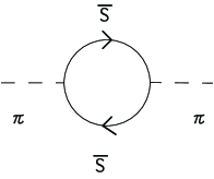
FIG. 2.: Fermion’s one loop contribution coming from the Yukawa interaction. The solid line is for the fermion $\Psi_{M}$, the dashed line for $\pi$ or $\sigma$.

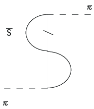
FIG. 3.: Fermion’s one loop contribution coming from the instantaneous interaction which is represented by the vertical solid line.

For simplicity, we put $k_{\bot}=0$. Using a parameter $x\equiv p^{+}/k^{+}$, the propagators $\Delta_{\pi,\sigma}(k)$ are expressed as

$$\frac{1}{N}\left(\matrix{\Delta_{\pi}^{-1}(k)\cr\Delta_{\sigma}^{-1}(k)}\right)=\frac{k^{2}}{\mu^{2}}-\frac{m^{2}_{\rm ZM}}{\mu^{2}}+{\cal F}(k^{2},M^{2})\left(\matrix{k^{2}\cr k^{2}-4M^{2}}\right),$$ (29)

$${\cal F}(k^{2},M^{2})\equiv\!\!\int_{0}^{1}\!\!dx\!\int\!\frac{d^{2}p_{\bot}}{(2\pi)^{3}}\frac{1}{p_{\bot}^{2}+M^{2}-k^{2}x(1-x)}$$ (30)

where we have utilized the gap equation (43) and $m_{\rm ZM}^{2}=\mu^{2}m/\lambda M$. The physical masses are determined from the equations $\Delta_{\sigma,\pi}^{-1}(k^{2}=m_{\sigma,\pi}^{2})=0$. Since the integral in ${\cal F}(k^{2},M^{2})$ diverges, we must specify a cutoff. Here we use the “extended PI cutoff” [10]:

$$\sum_{i}p_{\pm}^{(i)}<\Lambda,$$ (31)

where $i$ denotes the particles of the internal lines. This cutoff is a natural generalization of the naive PI cutoff $p_{\pm}<\Lambda$ and can be applied to multiple internal lines. In our case, the extended PI cutoff becomes

$$\frac{p_{\perp}^{2}+M^{2}}{x}+\frac{p_{\perp}^{2}+M^{2}}{1-x}<2\Lambda^{2}.$$

The explicit form of ${\cal F}(k^{2},M^{2})$ with this cutoff is given in Appendix E. Then we obtain highly complicated nonlinear equations for $m^{2}_{\pi,\sigma}$ which are also shown in Appendix E. First of all, it is almost trivial that the equation for $m_{\pi}$ has a solution $m_{\pi}=0$ in the chiral limit. For small bare mass $m\simeq 0$, we find

$$m_{\pi}^{2}=\frac{m}{\lambda M_{0}}\left[\frac{1}{\mu^{2}}+{\cal F}_{\rm EPI}(k^{2}\rightarrow 0,M_{0}^{2})\right]^{-1}+O(m^{2}),$$ (32)

where $M_{0}$ is a fermion condensate in the chiral limit and ${\cal F}_{\rm EPI}(k^{2}\rightarrow 0,M_{0}^{2})$ is independent of $m$ (see Appendix E). Therefore we have checked that the mass of the pion goes to zero in the chiral limit and now we can identify it with the NG boson.

The mass of $\sigma$ is determined in the same way. For example, in the chiral and heavy mass limit $m\rightarrow 0,\mu\rightarrow\infty$, one can easily find a solution $m_{\sigma}^{2}=(2M)^{2}$ which is known to exist in the NJL model in the chiral limit.

Our result of the pion mass (32) satisfies the Gell-Mann-Oakes-Renner (GOR) relation when $\mu\rightarrow\infty$:

$$m^{2}_{\pi}f_{\pi}^{2}=-4m\langle\bar{\Psi}\Psi\rangle,$$ (33)

where $f_{\pi}$ is the pion decay constant. To see this, let us calculate $f_{\pi}$ explicitly. Rewriting the pion’s propagator in the chiral and heavy scalar limit as

$$\Delta_{\pi}(k) = \frac{Z_{\pi}}{k^{2}-m_{\pi}^{2}},$$ (34)

$$Z_{\pi} \equiv \left[N{\cal F}_{\rm EPI}(k^{2}\rightarrow 0,M_{0}^{2})\right]^{-1},$$ (35)

we find the the effective pion-quark coupling $g_{\pi}=\sqrt{Z_{\pi}}$. Then, in the leading order of $1/N$ expansion, $f_{\pi}$ is given by a fermion one-loop integral with appropriate Lorentz structure:

$$ik^{\mu}f_{\pi} \equiv -\left\langle 0\left|\ j^{\mu}_{5}(0)\ \right|\pi(k)\right\rangle$$ (36)

$$= g_{\pi}N\int\frac{d^{4}p}{(2\pi)^{4}}\ {\rm tr}\left[\gamma^{\mu}\gamma_{5}{\overline{S}}(p-k)\gamma_{5}{\overline{S}}(p)\right]$$ (37)

$$= 2ig_{\pi}NM_{0}k^{\mu}{\cal F}_{\rm EPI}(k^{2}\rightarrow 0,M_{0}^{2}),$$ (38)

therefore

$$f_{\pi}=2M_{0}\left[N{\cal F}_{\rm EPI}(k^{2}\rightarrow 0,M_{0}^{2})\right]^{1/2}=\frac{2M_{0}}{\sqrt{Z_{\pi}}}\ .$$ (39)

Using this result and $m_{\pi}^{2}=\frac{m}{\lambda M_{0}}NZ_{\pi}$, we finally confirm the GOR relation (33).

2 Symmetric phase

Next let us consider the symmetric case. Using the symmetric solution to the zero-mode constraint, we can evaluate the masses of $\sigma$ and $\pi$ in the symmetric phase. In the chiral limit, we have

$$\frac{1}{N}{\Delta_{\pi,\sigma}(k)}^{-1}=\frac{k^{2}}{\mu^{2}}-\frac{m^{2}_{\rm ZM}}{\mu^{2}}+{\cal F}(k^{2},M^{2}=0)k^{2}$$ (40)

where the zero-mode mass $m_{\rm ZM}^{2}$ in the symmetric phase is expressed differently from that in the broken phase: $m_{\rm ZM}^{2}=\frac{\mu^{2}}{\lambda}-\frac{\mu^{2}}{\lambda_{\rm cr}}+O(m)$. Since $\Delta_{\sigma}(k)=\Delta_{\pi}(k)$, $\sigma$ and $\pi$ have the same physical mass $m_{\pi}^{2}=m_{\sigma}^{2}$. The physical mass $m_{\pi}^{2}$ is obtained as a solution of

$$\frac{m_{\pi}^{2}}{\mu^{2}}+\left(\frac{1}{\lambda_{\rm cr}}-\frac{1}{\lambda}\right)=-m_{\pi}^{2}\frac{\pi}{(2\pi)^{3}}\ln\left|\frac{2\Lambda^{2}-m_{\pi}^{2}}{m_{\pi}^{2}}\right|.$$ (41)

In the region $\lambda\stackrel{{\scriptstyle<}}{{\sim}}\lambda_{\rm cr}$, there is a nonzero solution $m_{\pi}^{2}<2\Lambda^{2}$.

In FIG. 4, we show the square masses of $\sigma$ and $\pi$ around $\lambda\sim\lambda_{\rm cr}$ in the chiral and NJL limit ($m\rightarrow 0,\ \mu\rightarrow\infty$). In the broken phase ($\lambda>\lambda_{\rm cr}$), $m_{\pi}^{2}=0$ and $m_{\sigma}^{2}=(2M)^{2}$, while in the symmetric phase ($\lambda<\lambda_{\rm cr}$), $m_{\sigma}^{2}=m_{\pi}^{2}$ is given as a solution to Eq. (41). The pion mass $m_{\pi}^{2}$ goes to zero in the limit $\lambda\rightarrow\lambda_{\rm cr}-0$.

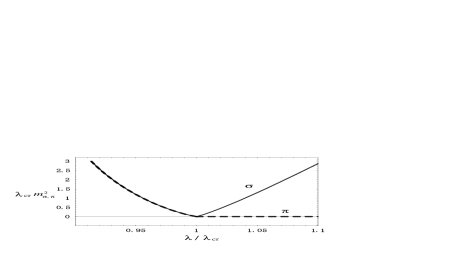
FIG. 4.: Squared masses $m^{2}_{\sigma,\pi}$ for $m\rightarrow 0$ and $\mu\rightarrow\infty$ scaled by $\lambda_{\rm cr}^{-1}$. Solid line is for $\sigma$ and dashed line for $\pi$. For $\lambda>\lambda_{\rm cr}$ we used the broken solution, whereas for $\lambda<\lambda_{\rm cr}$ symmetric solution.

It is important to recognize that Eq. (41) implies the existence of tachyonic modes for $\lambda>\lambda_{\rm cr}$ as we mentioned before. Indeed, if we assume $\lambda>\lambda_{\rm cr}$, we find a negative solution $m_{\pi}^{2}<0$. Therefore, if we choose the symmetric solution to the zero-mode constraint, then the resulting theory becomes unstable for $\lambda>\lambda_{\rm cr}$. So we must select the broken solution above the critical coupling.

C Derivation of the PCAC relation and the nonconservation of $Q_{5}^{\rm LF}$

As we discussed in Sec. III-B2, it is almost hopeless to treat the LF chiral current $\widehat{j}_{5}^{\mu}$ for the massive case. Instead, we adopt the current $j_{5}^{\mu}$ (8) which is much more tractable than $\widehat{j}_{5}^{\mu}$ and gives the same null-plane charge. Then it is straightforward to derive the PCAC relation. Consider the divergence of $j_{5}^{\mu}$ in the $\mu\rightarrow\infty$ limit [see Eq. (13) ]

$$\partial_{\mu}j^{\mu}_{5} = -2m\bar{\Psi}i\gamma_{5}\Psi$$ (42)

$$= 2m\frac{N}{\lambda}\ \pi$$ (43)

$$= 2m\frac{N}{\lambda}\sqrt{Z_{\pi}}\ \pi_{\rm n},$$ (44)

where the normalized pion field $\pi_{\rm n}$ was introduced so that its propagator be $\Delta_{\pi}^{\rm(n)}(k)=1/(k^{2}-m_{\pi}^{2})$ [see Eq. (34)]. If we use the pion decay constant (39) and the pion mass (32) [or equivalently $m_{\pi}^{2}=\frac{m}{\lambda M_{0}}NZ_{\pi}$], we obtain the PCAC relation,

$$\partial_{\mu}j^{\mu}_{5}=m_{\pi}^{2}f_{\pi}\pi_{\rm n}.$$ (45)

This is also consistent with Eq. (38) [our normalization is $\langle 0|\pi_{\rm n}|\pi(k)\rangle=1$].

The important consequences of Sec. V-A were that i) the null-plane chiral charge $Q_{5}^{\rm LF}$ is not conserved in the broken phase $\left[Q_{5}^{\rm LF},H_{\rm LF}\right]\neq 0$, and that ii) the violation is proportional to the dynamical fermion mass $M$ and does not disappear even in the chiral limit. Since we did not show explicitly the quantity because of its complexity, we here discuss it in more elegant way in the context of the PCAC relation. First of all, let us remember that the chiral charge (9) defined by $j_{5}^{\mu}$ is equivalent to the one defined from $\widehat{j}_{5}^{\mu}$ due to $\widehat{j}_{5}^{+}=j_{5}^{+}$. This means that the time derivative of $Q_{5}^{\rm LF}$ should be the same even if we use the current $j_{5}^{\mu}$. Therefore, we can calculate the quantity $\partial_{+}Q_{5}^{\rm LF}$ from the PCAC relation (45):

$$\partial_{+}Q_{5}^{\rm LF} = \frac{1}{i}\left[Q_{5}^{\rm LF},H_{\rm LF}\right]$$ (46)

$$= f_{\pi}m_{\pi}^{2}\int dx^{-}d^{2}x_{\perp}\pi_{\rm n}$$ (47)

$$= f_{\pi}m_{\pi}^{2}\int dx^{-}d^{2}x_{\perp}\pi_{\rm n}^{0},$$ (48)

where $\pi_{\rm n}^{0}$ is the zero mode of $\pi_{\rm n}$. If the current mass is not zero, the r.h.s. does not vanish in general and the chiral charge $Q_{5}^{\rm LF}$ does not conserve. Since the r.h.s. is proportional to $m_{\pi}^{2}$, it seems vanish in the chiral limit $m_{\pi}^{2}\propto m\rightarrow 0$. However, it does survive finite even in the chiral limit because the pion zero mode shows the singular behavior in the chiral limit:

$$\int dx^{-}d^{2}x_{\perp}\pi_{\rm n}^{0}\propto\frac{1}{m}\ .$$ (49)

Since $f_{\pi}$ is proportional to the fermion’s dynamical mass $M_{0}$ [Eq. (39)], we can confirm the result in Sec. V-A. That is, the null-plane chiral charge $Q_{5}^{\rm LF}$ does not conserve $\partial_{+}Q_{5}^{\rm LF}\neq 0$ even in the chiral limit. The singular behavior of Eq. (49) in the chiral limit has been pointed out by Tsujimaru and Yamawaki for spontaneously broken theories[23]. They showed the necessity of introducing the nonzero mass $m_{\rm NG}\neq 0$ for the NG boson in the broken phase and found the singular behavior of the NG-boson zero mode $\phi_{0}^{\rm NG}$ as

$$\int dx^{-}d^{2}x_{\perp}\phi_{0}^{\rm NG}\sim\frac{1}{m_{\rm NG}^{2}}.$$

We have confirmed their result for the $dynamically$ broken theory.

Now let us verify the singular behavior (49). It is generally known that the zero-mode constraint for the NG boson becomes inconsistent in the broken phase unless we introduce finite mass of the NG boson by hand as regularization [23]. Using the zero-mode mass (52), the zero-mode constraint for $\pi_{0}$ is simply written as

$$\left(m_{\rm ZM}^{2}-\partial^{2}_{\perp}\right)\pi_{0}=\int_{-L}^{L}dx^{-}\mu^{2}f(x^{-},x_{\perp}).$$ (50)

Suppose $m_{\rm ZM}=0$ and introduce the periodic boundary condition on $\pi_{0}$ in the transverse directions, then the transverse integral $\int d^{2}x_{\perp}$ of the zero-mode constraint leads to inconsistency $0=\int d^{2}x_{\perp}\int_{-L}^{L}dx^{-}\mu^{2}f(x^{-},x_{\perp})\neq 0$, which suggests to introduce “zero-mode mass” $m_{\rm ZM}\neq 0$. In our calculation, the origin of the the finite mass of the NG boson is the fermion’s bare mass $m$ [not the scalar mass $\mu/\sqrt{\lambda}$]. Indeed, $m_{\rm ZM}^{2}=\mu^{2}m/\lambda M$ in the broken phase. Therefore in the $\mu\rightarrow\infty$ limit, we find the singular behavior of the zero mode:

$$\pi_{0} = \frac{1}{m_{\rm ZM}^{2}-\partial_{\perp}^{2}}\int_{-L}^{L}dx^{-}\mu^{2}f(x^{-},x_{\perp})$$ (51)

$$\rightarrow \frac{\lambda M}{m}\int_{-L}^{L}dx^{-}f(x^{-},x_{\perp}).$$ (52)

On the other hand, in the symmetric phase $m_{\rm ZM}^{2}=\mu^{2}(\frac{1}{\lambda}-\frac{1}{\lambda_{\rm cr}})+O(m)$ survives finite in the chiral limit. We called $m_{\rm ZM}$ “zero-mode mass”, but it should not be confused with the physical pion mass $m_{\pi}$. Both become nonzero due to nonzero bare mass $m\neq 0$, but we have to calculate fermion’s one loop to obtain the physical pion mass $m_{\pi}$.

VI Conclusion and discussions

We have studied a method of describing the dynamical chiral symmetry breaking on the LF. Our description is based on the idea in DLCQ that the symmetry breaking is achieved by solving the “zero-mode constraints”, which already succeeded to some extent in describing the spontaneous symmetry breaking in simple scalar models. The point is that we can utilize this idea even for the dynamical symmetry breaking in fermionic systems if we introduce bosonic auxiliary fields for $\bar{\Psi}\Psi$ and $\bar{\Psi}i\gamma_{5}\Psi$, and treat them as dynamical variables by adding their kinetic terms. Then the problem can be formulated such that we find a nontrivial solution to the “zero-mode constraint”. We exemplified this idea in the NJL model. The model we studied is the chiral Yukawa model, which reproduces the NJL model in the infinitely heavy mass limit of the scalars. Within this model, we showed in the massless case the equivalence between “light-front” chiral transformation and the usual one by classically solving the three (i.e. two zero-mode and one fermionic) constraints. This allowed us to construct the chiral current $j^{5}_{\mu}$ and charge $Q_{5}^{\rm LF}$. Even if we solve the constraints classically, the resulting theory cannot have a symmetry breaking term. Quantum analysis showed that the zero-mode constraint for a scalar boson $\sigma$ became the gap equation in nonperturbative treatment, which lead to nonzero condensate $\langle\sigma\rangle\neq 0$ and equivalently to the chiral symmetry breakdown. We found the critical coupling $\lambda_{\rm cr}$ beyond which the fermion acquires nonzero dynamical mass. On the other hand, a perturbative solution could not give fermion condensate even in the quantum theory.

The most important key of our description was the identification of the zero-mode constraint of $\sigma$ with the gap equation. This was suffered from a severe problem that the correct mass dependence disappears from the mode expansion. Of course this is a demerit of the LF formalism and we have to carefully incorporate mass dependence into e.g. $\langle\bar{\Psi}\Psi\rangle$ when we regularize its infrared divergence. It is suggestive that cutoff schemes with symmetry consideration such as parity or rotational invariance lead to physically acceptable results. Contrary to such negative aspects, the mass-information loss has a useful and important aspect. It follows that the Fock vacuum keeps invariant even if we change the value of mass. Therefore the vacuum does not change even though symmetry breaking occurs and the fermion acquires dynamical mass.

In our formalism, the vacuum is exactly the Fock vacuum. The inclusion of dynamical scalar fields was necessary to clarify the structure of the Hilbert space and the triviality of the vacuum. The way of realizing broken phase is that the vacuum is still trivial but the operator structure of the dependent variables changes. In other words, the “vacuum physics” in conventional formulation is converted into the hamiltonian through the dependent variables. The zero modes of scalars and the bad component $\psi_{-}$ are constrained variables and differently expressed by physical variables depending on the phases. Related to this, the LF chiral transformation of the dependent variables also becomes unusual in the broken phase. Consequently, a seemingly contradiction between the triviality of the null-plane charge $Q_{5}^{\rm LF}|0\rangle=0$ and the chiral condensate $\langle\bar{\Psi}\Psi\rangle\neq 0$ is resolved.

We further calculated masses of $\pi$ and $\sigma$ for both symmetric and broken phases. In the broken phase, the mass of $\pi$ goes to zero in the chiral limit, which is consistent with the NG theorem. Our result is consistent with the GOR relation. If we substitute symmetric solution into the lagrangian, there appear tachyon modes for $\lambda>\lambda_{\rm cr}$. Therefore we can say that when $\lambda>\lambda_{\rm cr}$, physically realized phase is the broken phase. Certainly we have massless pion in the model, but it is very difficult to verify the NG theorem in general on the LF. This is because we have nonlocal interaction and because the chiral transformation of the full fields explicitly depends on the model. Both of these arise from the fact that in the LF formalism the bad component of fermion and zero modes of scalars are constrained variables. However, we have succeeded in deriving the PCAC relation. This was enabled by utilizing the current $j_{5}^{\mu}$ which was the Noether current defined for the massless fermion. The ’massive’ current $\widehat{j}_{5}^{\mu}$ becomes complicated and it is almost hopeless to deal with it. The physics meaning of this discrepancy between $j_{5}^{\mu}$ and $\widehat{j}_{5}^{\mu}$ is still not clear but it seems that the usual current $j_{5}^{\mu}$ is favorable for discussing the “usual” chiral symmetry (not the “LF” chiral symmetry).

One of the most important conclusion of our analysis is the nonconservation of the LF chiral charge $Q_{5}^{\rm LF}$. This can be shown both by direct calculation of $[Q_{5}^{\rm LF},H_{\rm LF}]$ using the unusual chiral transformation law and by utilizing the PCAC relation. In the broken phase, the chiral charge $Q_{5}^{\rm LF}$ does not conserve $\partial_{+}Q_{5}^{\rm LF}\neq 0$ even in the chiral limit. The singular behavior $1/m$ of the pion zero mode is essential to give a finite violation of $\partial_{+}Q_{5}^{\rm LF}\neq 0$.

In our calculation, “nonperturbative” implied the mean-field approximation. This mean-field calculation is justified as the leading order approximation in the $1/N$ expansion. In principle, we can develop a systematic $1/N$ expansion to go beyond the mean-field result. Nevertheless, the higher order will severely depend on the operator ordering and it is not clear whether the result with our specific ordering makes sense. If we want to go beyond the leading order, we have to determine the consistent operator ordering according to the criterion discussed in the text. Since this is a very difficult task in our model, it should be examined in much simpler models such as 1+1 dimensional Yukawa theory.

It will be challenging to use other nonperturbative method to solve the zero-mode constraint. For example, Tamm-Dancoff approximation which truncates the Fock space into a few particle states will give some nontrivial results. Notice that our leading $1/N$ approximation corresponds to the two body truncation since multiquark states give higher order contribution.

Our method here heavily relies on the introduction of auxiliary fields. So it seems natural to ask a question: Can we describe the chiral symmetry breaking without introducing the auxiliary fields? The answer is of course yes. Even though we do not have zero mode constraints, it is possible to describe the chiral symmetry breaking on the LF. Its explicit demonstration in the purely fermionic NJL model will be given in our next paper [12]. As far as the NJL model is concerned, to solve the fermionic constraint becomes of great importance.

There still remain many problems which cannot be discussed in our model. One of them is the issue of renormalization. In a renormalizable theory, if one introduces an infrared cutoff and excludes the zero mode degrees of freedom from the beginning, then the “vacuum physics” should be discussed as the problem of renormalization with nonperturbative infrared counter terms. Relation between such counter term approach [25] and the zero-mode approach presented here is not clear. We need further investigation for understanding how to describe the chiral symmetry breaking in LFQCD.

A The chiral Yukawa model

Effective potential for scalars in the chiral Yukawa model (2) is easily calculated in the leading order of $1/N$ expansion [16]. Exactly in the same way as in the Gross-Neveu model [26], we find that the leading contribution comes from the fermion one-loop diagrams. Note that the inclusion of kinetic terms for scalars has no effect on the leading effective potential. Since the scalar propagator is $O(1/N)$, effects of the kinetic term (i.e. $\mu$ dependence) emerges from the next leading order. The effective potential $V(\sigma,\pi)$ in the leading order is independent of $\mu$ and is given by

$$V(\sigma,\pi)/N= \frac{1}{2\lambda}(\sigma^{2}+\pi^{2})$$ (A2)

$$+\ i\int\frac{d^{4}k}{(2\pi)^{4}}\ln\det[k\!\!\!/-(\sigma+i\gamma_{5}\pi)],$$

which is the same result as that of the NJL model. Therefore evaluating the integral and differentiating $V(\sigma,\pi=0)$ with respect to $\sigma$, we obtain the gap equation which determines the vacuum expectation value of $\sigma$.

Now let us turn to the mean-field approximation. Using $AB\approx\langle A\rangle B+A\langle B\rangle-\langle A\rangle\langle B\rangle$, the Yukawa interaction becomes

$$-{\cal L}_{\rm Yukawa}$$ (A3)

$$\quad\approx\langle\sigma\rangle\bar{\Psi}\Psi+\sigma\langle\bar{\Psi}\Psi\rangle+\langle\pi\rangle\bar{\Psi}i\gamma_{5}\Psi+\pi\langle\bar{\Psi}i\gamma_{5}\Psi\rangle+\ {\rm const.},$$ (A4)

where $\langle\sigma\rangle=O(N^{0}),\ \sigma-\langle\sigma\rangle=O(N^{-1/2})$ and similarly for others. The leading order Euler-Lagrange equations for $\sigma$ and $\pi$ are $\langle\sigma\rangle=-\frac{\lambda}{N}\langle\bar{\Psi}\Psi\rangle$ and $\langle\pi\rangle=-\frac{\lambda}{N}\langle\bar{\Psi}i\gamma_{5}\Psi\rangle$. Therefore, in the mean-field approximation (=leading order of $1/N$ expansion), the chiral Yukawa model allows both fermion and scalar condensates. However, in higher order, fermion bilinears and scalars can independently take their VEVs and the same relations do not necessarily hold. The Euler-Lagrange equation for fermion in the mean-field approximation becomes $(i\partial\!\!\!/-m-\langle\sigma\rangle-\langle\pi\rangle i\gamma_{5})\Psi=0$. Evaluating the fermion condensate in a self-consistent way, we obtain the gap equation.

B Conventions

We summarize our convention. We follow the Kogut-Soper convention [4]. First of all, the light-front coordinates are defined as

$$x^{\pm}=\frac{1}{\sqrt{2}}(x^{0}\pm x^{3}),\quad x^{i}_{\perp}=x^{i}\quad(i=1,2),$$ (B1)

where we treat $x^{+}$ as “time”. The spatial coordinates $x^{-}$ and $x_{\perp}$ are called the longitudinal and transverse directions respectively. Derivatives in terms of $x^{\pm}$ are defined by

$$\partial_{\pm}\equiv\frac{\partial}{\partial x^{\pm}}.$$ (B2)

For the $\gamma$ matrices, we also define

$$\gamma^{\pm}=\frac{1}{\sqrt{2}}(\gamma^{0}\pm\gamma^{3}).$$ (B3)

It is useful to introduce projection operators $\Lambda_{\pm}$ defined by

$$\Lambda_{\pm}=\frac{1}{2}\gamma^{\mp}\gamma^{\pm}=\frac{1}{\sqrt{2}}\gamma^{0}\gamma^{\pm}.$$ (B4)

Indeed $\Lambda_{\pm}$ satisfy the projection properties $\Lambda_{\pm}^{2}=\Lambda_{\pm},\ \Lambda_{+}+\Lambda_{-}=1$, etc. Splitting the fermion by the projectors,

$$\Psi^{a}=\psi^{a}_{+}+\psi^{a}_{-},\quad\psi^{a}_{\pm}\equiv\Lambda_{\pm}\Psi^{a},$$ (B5)

we find that for any fermion on the LF, $\psi_{-}$ component is a dependent degree of freedom. $\psi_{+}$ and $\psi_{-}$ are called the “good component” and the “bad component”, respectively.

In DLCQ, we set $x^{-}$ finite $x^{-}\in[-L,L]$ with some boundary conditions on fields. Taking the periodic boundary condition, we can clearly separate a longitudinal zero mode from oscillating modes. The zero mode of some local function $f(x)$ is defined by

$$f_{0}(x_{\perp})=\frac{1}{2L}\int_{-L}^{L}dx^{-}f(x^{-},x_{\perp}).$$ (B6)

The rest is the oscillating part:

$$\varphi_{f}(x)=f(x)-f_{0}(x_{\perp}).$$ (B7)

For some composite fields, we use the notation $[\quad]_{0}$ for their zero modes:

$$\Big{[}f(x)g(x)\Big{]}_{0}=\frac{1}{2L}\int_{-L}^{L}dx^{-}f(x)g(x).$$ (B8)

The inverse of the differential operator $\partial_{-}$ is defined as

$$\frac{1}{\partial_{-}}f(x^{-})\equiv\int_{-L}^{L}dy^{-}\frac{1}{2}\epsilon(x^{-}-y^{-})f(y^{-}),$$ (B9)

where $\epsilon(x^{-})$ is a sign function

$$\epsilon(x^{-})=\left\{\matrix{1\quad(x^{-}>0)\cr 0\quad(x^{-}=0)\cr-1\quad(x^{-}<0)}\right..$$ (B10)

C Constraints and Their Classical Solutions

Since systems on the LF always have several constraints, the LF quantization must be performed using Dirac’s Hamiltonian formalism for constrained systems.

The chiral Yukawa model has six primary constraints. Among them, consistency conditions for $\theta_{1}=\Pi_{\sigma_{0}}\approx 0$ and $\theta_{2}=\Pi_{\pi_{0}}\approx 0$ ($\Pi_{\Phi}$ is a conjugate momenta of $\Phi$) generate the zero-mode constraints (3), while $\theta_{3}=\Pi_{\psi_{-}}\approx 0$ generates the fermionic constraint (1). The consistency is calculated by $\dot{\theta}_{i}=\{\theta_{i},H_{\rm LF}+\lambda_{j}\theta_{j}\}_{\rm PB}\approx 0$ with the canonical light-front Hamiltonian $H_{\rm LF}=P^{-}$

$$P^{-} =P^{-}_{\rm F}+P^{-}_{\rm B}+P^{-}_{\rm Y},$$ (C6)

$$P^{-}_{\rm F}=\int d^{3}x\left\{-\bar{\Psi}^{a}i\gamma^{-}\partial_{-}\Psi^{a}-\bar{\Psi}^{a}i\gamma^{\perp}\partial_{\perp}\Psi^{a}+m\bar{\Psi}^{a}\Psi^{a}\right\},$$

$$P^{-}_{\rm B}=\int d^{3}x\biggl{[}-{N\over 2\mu^{2}}\left\{(\partial^{\perp}\sigma_{0}\partial_{\perp}\sigma_{0}+\partial^{\perp}\varphi_{\sigma}\partial_{\perp}\varphi_{\sigma})\right.\biggr{.}$$

$$\hskip 79.6678pt\left.+(\partial^{\perp}\pi_{0}\partial_{\perp}\pi_{0}+\partial^{\perp}\varphi_{\pi}\partial_{\perp}\varphi_{\pi})\right\}$$

$$\hskip 54.06006pt\biggl{.}+{N\over 2\lambda}\left\{(\sigma_{0}^{2}+\varphi_{\sigma}^{2})+(\pi_{0}^{2}+\varphi_{\pi}^{2})\right\}\biggr{]},$$

$$P^{-}_{\rm Y}=\int d^{3}x\left\{(\sigma_{0}+\varphi_{\sigma})\bar{\Psi}^{a}\Psi^{a}+(\pi_{0}+\varphi_{\pi})\bar{\Psi}^{a}i\gamma_{5}\Psi^{a}\right\},$$

where $\int d^{3}x=\int_{-L}^{L}dx^{-}\int d^{2}x_{\perp}$. As a result, we find that no more constraints are generated from consistency conditions and that this system belongs to the second class.

If we ignore ordering of the variables, it is not difficult to solve the constraints. First, the fermionic constraint (1) is solved as

$$\psi^{a}_{-}=\frac{1}{i\partial_{-}}\left[{1\over 2}\left(i\gamma^{\perp}\partial_{\perp}+m+\sigma-i\pi\gamma_{5}\right)\gamma^{+}\psi^{a}_{+}\right]~{},$$ (C7)

where $\partial_{-}^{-1}$ is defined so that $\psi_{-}(x)$ also satisfies the antiperiodic boundary condition (see Appendix B). Note that however this solution still contains the zero modes $\sigma_{0}$ and $\pi_{0}$ and thus is not a complete solution. Substituting (C7) into Eq. (3), we have equations only for $\sigma_{0}$ and $\pi_{0}$. Then the formal solution is given by

$$\left(\matrix{\sigma_{0}(x_{\bot})\cr\pi_{0}(x_{\bot})}\right)$$ (C8)

$$=-{1\over\sqrt{2}}{\mu^{2}\over N}{\cal D}^{-1}(x_{\perp})\left[\psi_{+}^{a{\dagger}}\left(\matrix{-1\cr i\gamma_{5}}\right)\frac{1}{i\partial_{-}}(i\gamma^{\perp}\partial_{\perp}-m)\psi^{a}_{+}\right.$$ (C9)

$$\quad\quad\left.+\ \psi_{+}^{a{\dagger}}\frac{1}{i\partial_{-}}\left\{\left(\matrix{\varphi_{\sigma}+i\gamma_{5}\varphi_{\pi}\cr\varphi_{\pi}-i\gamma_{5}\varphi_{\sigma}}\right)\psi_{+}^{a}\right\}+\ {\rm c.c.}\ \right]_{0},$$ (C10)

where the transverse differential operator ${\cal D}(x_{\perp})$ is

$${\cal D}(x_{\perp})={\mu^{2}\over\lambda}+{\mu^{2}\over N}{1\over\sqrt{2}}\left[\psi_{+}^{a{\dagger}}\frac{1}{i\partial_{-}}\psi^{a}_{+}-\left(\frac{1}{i\partial_{-}}\psi_{+}^{a{\dagger}}\right)\psi^{a}_{+}\right]_{0}-\partial_{\bot}^{2}.$$

The final expression for $\psi_{-}$ is reached after we insert Eq. (C10) into Eq. (C7). Though we have completely ignored the “ordering” in the classical treatment, the operator ordering becomes an issue in a quantum theory, which makes the analysis very complicated.

D Perturbative Solution to the Zero-Mode Constraints in Quantum Analysis

Let us solve the zero-mode constraints in perturbation theory with the natural ordering in Eqs. (1) and (3). In addition to the expansions (21)-(23), it is convenient to define the expansion of $\Psi$:

$$\Psi^{a}=\sum_{n=0}^{\infty}\left(\frac{\lambda}{\lambda_{\rm cr}}\right)^{n}\Psi^{a(n)},$$ (D1)

where $\Psi^{a(0)}=\psi^{a}_{+}+\psi_{-}^{a(0)}$ and $\Psi^{a(k)}=\psi_{-}^{a(k)}$ for $k\geq 1$.

Knowing the lowest order solutions (25), we obtain the next order solution,

$$\left(\matrix{\sigma_{0}^{(1)}\cr\pi_{0}^{(1)}}\right)=-{\lambda_{\rm cr}\over N}\left[\bar{\Psi}^{a(0)}\left(\matrix{1\cr i\gamma_{5}}\right)\Psi^{a(0)}\right]_{0}~{},$$ (D2)

$$\psi_{-}^{a(1)}={1\over 2}{1\over i\partial_{-}}\left(\sigma_{0}^{(1)}-i\pi_{0}^{(1)}\gamma_{5}\right)\gamma^{+}\psi^{a}_{+}.$$ (D3)

Similarly, if we know the solution up to $n$-th order, we easily obtain the $(n+1)$-th order solution because the constraint equation is written as follows

$$\frac{\mu^{2}}{\lambda_{\rm cr}}\left(\matrix{\sigma_{0}^{(n+1)}\cr\pi_{0}^{(n+1)}}\right) = \partial_{\perp}^{2}\left(\matrix{\sigma_{0}^{(n)}\cr\pi_{0}^{(n)}}\right)$$ (D4)

$$- {\mu^{2}\over N}\left[\bar{\Psi}^{a(0)}\left(\matrix{1\cr i\gamma_{5}}\right)\Psi^{a(n)}+{\rm h.c.}\right]_{0},$$ (D5)

where $\Psi^{a(n)}$ for $n\neq 0$ is

$$\Psi^{a(n)}=\frac{1}{2}\frac{1}{i\partial_{-}}\left(\sigma_{0}^{(n)}-i\pi_{0}^{(n)}\gamma_{5}\right)\gamma^{+}\psi_{+}^{a},$$ (D6)

and we have used $\psi_{-}^{(k){\dagger}}\gamma^{0}\psi_{-}^{(l)}=0$ for $k,l\neq 0$, etc. In this way, we can determine the solution order by order.

E Nonlinear Equations for Pole Masses

With the Extended Parity Invariant (EPI) cutoff, the integral ${\cal F}(k^{2},M^{2})$ Eq. (30) is given as

$${\cal F}_{\rm EPI}(k^{2},M^{2}) \equiv \int_{x_{(-)}}^{x_{(+)}}dx\int_{0}^{2\Lambda^{2}x(1-x)-M^{2}}dp_{\bot}^{2}$$ (E2)

$$\quad\times\ \frac{\pi}{(2\pi)^{3}}\frac{1}{p_{\bot}^{2}+M^{2}-k^{2}x(1-x)}.$$

where integration limit $x_{(\pm)}=(1\pm\beta)/2$ with $\beta=\sqrt{1-2M^{2}/\Lambda^{2}}$ comes from $2\Lambda^{2}x(1-x)-M^{2}>0$. The integral is easily performed and the result is

$${\cal F}_{\rm EPI}(k^{2},M^{2})=\frac{1}{8\pi^{2}}\log\left(\frac{1+\beta}{1-\beta}\right)$$ (E3)

$$\quad-\frac{1}{4\pi^{2}}\sqrt{\frac{4M^{2}-k^{2}}{k^{2}}}\arctan\beta\sqrt{\frac{k^{2}}{4M^{2}-k^{2}}}.$$ (E4)

For $k^{2}\sim 0$, we can approximate this as

$${\cal F}_{\rm EPI}(k^{2}\rightarrow 0,M^{2})=\frac{1}{8\pi^{2}}\log\left(\frac{1+\beta_{0}}{1-\beta_{0}}\right)-\frac{1}{4\pi^{2}}\beta_{0},$$ (E5)

where $\beta_{0}=\sqrt{1-2M_{0}^{2}/\Lambda^{2}}$ and we used $\lim_{x\rightarrow 0}x^{-1}\arctan x=1$.

Using above, the nonlinear equations for the scalar masses are

$$\frac{m}{\lambda M}=\frac{1}{\mu^{2}}\left(\matrix{m_{\pi}^{2}\cr m_{\sigma}^{2}}\right)+\left(\matrix{m_{\pi}^{2}{\cal F}_{\rm EPI}(m_{\pi}^{2},M^{2})\cr(m_{\sigma}^{2}-4M^{2}){\cal F}_{\rm EPI}(m_{\sigma}^{2},M^{2})}\right).$$ (E6)

Note that when the chiral and heavy mass limit $m\rightarrow 0$, $\mu\rightarrow\infty$, we have solutions $m_{\pi}=0$ and $m_{\sigma}=2M$.

REFERENCES

- [1] For example, V.A. Miransky, “Dynamical Symmetry Breaking in Quantum Field Theories” (World Scientific, 1993), M.A. Nowak, M. Rho, and I. Zahed, “Chiral Nuclear Dynamics” (World Scientific, 1996).
- [2] Y. Nambu and G. Jona-Lasinio, Phys. Rev. 122, 345 (1961).
- [3] T. Hatsuda and T. Kunihiro, Phys. Rep. 247, 221 (1994), S.P. Klevansky, Rev. Mod. Phys. 64, 649 (1992), U. Vogl and W. Weise, Prog. Part. Nucl. Phys. 27, 195 (1991).
- [4] S.J. Brodsky, H.C. Pauli and S.S. Pinsky, Phys. Rep. 301, 299 (1998).
- [5] T. Heinzl, S. Krusche, S. Simburger and E. Werner, Z. Phys. C56, 415 (1992); T. Heinzl, C. Stern, E. Werner and B. Zellermann, Z. Phys. C72, 353 (1996); D.G. Robertson, Phys. Rev. D47, 2549 (1993); C.M. Bender, S. Pinsky and B. van de Sande, Phys. Rev. D48, 816 (1993); S. Pinsky and B. van de Sande, Phys. Rev. D49, 2001 (1994); S. Pinsky, B. van de Sande and J.R. Hiller, Phys. Rev. D51, 726 (1995).
- [6] T. Maskawa and K. Yamawaki, Prog. Theor. Phys. 56, 270 (1976); H.C. Pauli and S.J. Brodsky, Phys. Rev. D32, 1993 (1985); ibid. D32, 2001 (1985).
- [7] C. Dietmaier, et al. Z. Phys. A334, 215 (1989).
- [8] K. Itakura, “Toward a Description of Broken Phases in Light-Front Field Theories” Ph.D. Thesis (University of Tokyo, December 1996); K. Itakura, Prog. Theor. Phys. 98, 527 (1997).
- [9] T. Heinzl, “Light-Cone Dynamics of Particles and Fields” hep-th/9812190 (unpublished).
- [10] T. Hama, “The Nambu-Jona-Lasinio Model on the Light-Cone and Its Application to Structure Functions” Master Thesis, (University of Tokyo, 1998); W. Bentz, et al., Nucl. Phys. A651, 143 (1999).
- [11] K. Itakura and S. Maedan, Prog. Theor. Phys. 97, 635 (1997).
- [12] K. Itakura and S. Maedan, “Dynamical Chiral Symmetry Breaking on the Light Front II. NJL Model in the Continuum Approach” (in preparation).
- [13] D. Mustaki, “Chiral Symmetry and the Constituent Quark Model: A Null-Plane Point of View” hep-ph/9404206 (unpublished).
- [14] M. Gell-Mann and M. Lévy, Nuovo Cim. 16, 705 (1960); B. Lee, “Chiral Dynamics” (Gordon and Breach, 1972).
- [15] R. Carlitz, et al. Phys. Rev. D11, 1234 (1975).
- [16] T. Kugo, “Effective Action and Spontaneous Symmetry Breaking” Ph. D. Thesis (Kyoto Univ. 1976), also in Soryushiron Kenkyu 53, 1 (1976) [in Japanese].
- [17] For example, A. Manohar and H. Georgi, Nucl. Phys. B234, 189 (1984).
- [18] N. Nakanishi and K. Yamawaki, Nucl. Phys. B122, 15 (1977).
- [19] H. Leutwyler, “Current Algebra and Lightlike Charges” in Springer Tracts in Modern Physics, No. 50, (Springer, New York, 1969).
- [20] D.K. Kim, Y.D. Han, and I.G. Koh, Phys. Rev. D49, 6943 (1994).
- [21] T. Heinzl, Phys. Lett. B388, 129 (1996).
- [22] J. Jersak and J. Stern, Nucl. Phys. B7, 413 (1968); A. Casher, S.H. Noskowicz, and L. Susskind, Nucl. Phys. B32, 75 (1971); M. Ida, Prog. Theor. Phys. 51, 1521 (1974).
- [23] Y. Kim, S. Tsujimaru and K. Yamawaki, Phys. Rev. Lett. 74, 4771 (1995); S. Tsujimaru and K. Yamawaki, Phys. Rev. D57, 4942 (1998).
- [24] S-J. Chang, R.G. Root, and T-M. Yan, Phys. Rev. D7, 1133 (1973); S-J. Chang, and T-M. Yan, Phys. Rev. D7, 1147 (1973); T-M. Yan, Phys. Rev. D7, 1760 (1973); ibid. D7, 1780 (1973).
- [25] M. Burkardt and H. El-Khozondar, Phys. Rev. D55, 6514 (1997); M. Burkardt, Phys. Rev. D58, 096015 (1998).
- [26] D.J. Gross and A. Neveu, Phys. Rev. D10, 3235 (1975).