hep-th/9907068

Vortex String Dynamics

in an External Antisymmetric Tensor Field

Kimyeong Lee, Q-Han Park and H.J. Shin

¹Physics Department and CTP, Seoul National University, Seoul 130-743, Korea

^2,3Department of Physics and Research Institute of Basic Science

Kyung Hee University, Seoul 130-701, Korea

ABSTRACT

We study the Lund-Regge equation that governs the motion of strings in a constant background antisymmetric tensor field by using the duality between the Lund-Regge equation and the complex sine-Gordon equation. Similar to the cases of vortex filament configurations in fluid dynamics, we find various exact solitonic string configurations which are the analogue of the Kelvin wave, the Hasimoto soliton and the smoke ring. In particular, using the duality relation, we obtain a completely new type of configuration which corresponds to the breather of the complex sine-Gordon equation.

1 Introduction

There has been some studies on the dynamics of a string coupled to an antisymmetric tensor field. Such a coupling was first introduced by Kalb and Ramond in the context of string theory [1]. It also appears in the study of the relativistic motion of vortex strings in a superfluid by Lund and Regge [2], where the antisymmetric tensor field induces the Magnus force acting on the vortex string by uniform fluid density. In particular, Lund and Regge has shown that the dynamical equation for vortex strings can be ‘dualized’ to the complex sine-Gordon equation [2], and they have also found a soliton solution of the complex sine-Gordon equation. More recently, using a simple ansatz, Zee found the smoke ring solution of the Lund-Regge equation [3]. However, despite the dualization of the Lund-Regge equation to the complex sine-Gordon equation, which is exactly integrable with many known exact solutions, nothing much is known about the exact solutions of the Lund-Regge equation itself.

In the context of fluid dynamics, we encounter vortex filaments in an incompressible inviscid fluid [4]. The relevant dynamics of vortex filaments is described in terms of variables ${\bf X}(\tau,\sigma)$, which represent the vortex position where $\sigma$ measures the length of the vortex filament. When we neglect both vortex mass and long range interaction, and also introduce a short-distance cutoff, the dimensionless form of the dynamical equation for the vortex $X(\tau,\sigma)$ becomes the Da Rios-Betchov equation [5]:

$$\dot{\bf X}={\bf X}^{\prime}\times{\bf X}^{\prime\prime}$$ (1)

where the dot denotes $\partial/\partial\tau$ and the prime denotes $\partial/\partial\sigma$. Various exact solutons of the Da Rios-Betchov equation are known and their stability properties have been analyzed. Among many solutions, the Kelvin wave, a helical configuration of vortex filament, and the smoke ring solutions arise as simple cases. Another interesting solution is the solitary kink wave which propagates along a straight vortex filament line. This was first found by Hasimoto [6] by mapping the Da Rios-Betchov equation into the nonlinear Schrödinger (NLS) equation and finding soliton solutions of the NLS equation. The stability of the Kelvin wave has been also studied [7]. There are also more recent studies of this equation [8].

In the case of the Lund-Regge equation, the smoke ring solution found by Zee suggests that other types of solitonic solutions might exist as well. Moreover, the duality between the Lund-Regge and the complex sine-Gordon equations implies that exact solutions, e.g. solitons [2], of the complex sine-Gordon equation have counterparts in the vortex system. So far, however, explicit expressions of these solutions have not been known despite of the dualization of the Lund-Regge equation to the integrable complex sine-Gordon equation. This is mainly due to the fact that the duality relation between two equations obtained by Lund and Regge is incomplete. That is, their dualization is only one-directional: it allows us to express the variables of the complex sine-Gordon equation in terms of those of the Lund-Regge equation but not vice versa. Recently, the reverse direction has been found by utilizing the associated linear equation of the complex sine-Gordon equation, in addition with an abstract generalization of the Lund-Regge equation using group theory [9].

In this paper, we analyze the Lund-Regge model using its dualization to the complex sine-Gordon model. The duality between these two models is explained in detail in terms of the $SU(2)/U(1)$-gauged Wess-Zumino-Novikov-Witten (WZNW) model with a potential term. This allows us to understand symmetries of the Lund-Regge model from different perspectives. By making use of exact solutions of the complex sine-Gordon equation, we find various vortex-type configurations of the Lund-Regge equation similar to vortex filament configurations in fluid dynamics such as the Kelvin wave, the smoke ring, and the Hasimoto soliton. In particular, we obtain the breather-type vortex solution by dualizing the breather solution of the complex sine-Gordon equation.

The plan of this paper is as follows. In Sec. 2, we review the Lund-Regge model and its relation to the complex sine-Gordon model. In Sec. 3, we explain about the Wess-Zumino-Novikov-Witten sigma model formulation of the complex sine-Gordon model, and derive exact solutions of the complex sine-Gordon equation using the Bäcklund transformation. In Sec. 4, we dualize these solutions to the configurations of vortex strings. We obtain the smoke ring, Kelvin wave, Hasimoto soliton, and the breather. We conclude with some remarks in Sec. 5.

2 The Lund-Regge Model

The dynamics of a charged particle in an external electromagnetic field is determined by a Lorentz force acting on a particle. From the view point of a particle Lagrangian, this is done by coupling the vector gauge potential of electromagnetism to a charged particle in a gauge invariant way. In the case of string dynamics in an external field, the antisymmetric tensor field $B_{\mu\nu}$ plays the role of a gauge connection for string and the corresponding field strength ($H=dB$) induces the Magnus force acting on string. In physical applications, the antisymmetric tensor field is not a fundamental physical variable such as the vector gauge potential but appears as an effective description of external fields. For example, the vortex string in an idealized superconductor in zero temperature is described by a Maxwell-Higgs system with a uniform external electric charge density [10]. In this case, the Magnus force is generated by the electric charge of the Higgs field which neutralizes the background charge. In the following, we will not concern about any specific physical applications. Instead, we regard the antisymmetric tensor field simply as an external field appearing in the context of a string theory.

The Lagrangian for the string coupled to an antisymmetric tensor field is given by

$${\cal L}_{\rm string}=-{\mu\over 2}\partial^{\alpha}X^{\mu}\partial_{\alpha}X_{\mu}+B_{\mu\nu}\epsilon^{\alpha\beta}\partial_{\alpha}X^{\mu}\partial_{\beta}X^{\nu},$$ (2)

where $(\tau,\sigma)$ is the string world-sheet coordinates and $\alpha=\tau,\sigma;~{}\mu=0,1,2,3.$ The string tension is given by $\mu$. Here, we only consider the closed string or the infinite size string without any ends. This Lagrangian is invariant under the conformal transformation $\tau\pm\sigma\rightarrow f_{\pm}(\tau\pm\sigma)$ where $f_{\pm}$ are arbitrary functions. The conformal symmetry results in a constraint as the vanishing of the two dimensional energy-momentum tensor,

$$\ \dot{X}^{\mu}\dot{X}_{\mu}+\ X^{\prime\mu}X^{\prime}_{\mu}=0,$$

$$\ \dot{X}^{\mu}X^{\prime}_{\mu}=0.$$ (3)

On the other hand, the classical equation for the string coming from the variation on $X^{\mu}$ is

$$\mu\partial_{\alpha}^{2}X^{\mu}=H^{\mu\nu\rho}\epsilon^{\alpha\beta}\partial_{\alpha}X_{\nu}\partial_{\beta}X_{\rho},$$ (4)

where $H_{\mu\nu\rho}\equiv\partial_{\mu}B_{\nu\rho}+\partial_{\nu}B_{\rho\mu}+\partial_{\rho}B_{\mu\nu}$ is the gauge invariant field strength of $B_{\mu\nu}$. The Magnus force acting on the string is a stringy generalization of the Lorentz force, and appears in the literature in many disguise. In particular, Lund and Regge have shown that the relativistic motion of vortices in a uniform static field $H$ is described precisely in this way; in a Lorentz frame in which $X^{0}=\tau$, the system is governed by the gauge fixed equation of motion,

$$(\partial_{\tau}^{2}-\partial_{\sigma}^{2})X^{i}+c\epsilon_{ijk}\partial_{\tau}X^{j}\partial_{\sigma}X^{k}=0,~{}~{}i=1,2,3$$ (5)

where $H_{ijk}=c\mu\epsilon_{ijk}$, and also by the quadratic constraints:

$$(\partial_{\tau}X^{i})^{2}+(\partial_{\sigma}X^{i})^{2}=1,~{}~{}(\partial_{\sigma}X^{i})(\partial_{\tau}X^{i})=0.$$ (6)

Here, $X^{i}(\sigma,\tau);i=1,2,3$ are the vortex coordinates and $\sigma,~{}\tau$ are local coordinates on the string world-sheet. In the no-coupling limit ($c=0$), this equation describes the transverse modes of the 4-dimensional Nambu-Goto string in the orthonormal gauge. The critical step leading to the integration of the vortex equation (5) and (6) is to interpret the equation as the Gauss-Codazzi integrability condition for the embedding of a surface, i.e. the embedding of the string world-sheet projected down to the $X^{0}=\tau$ hypersurface into the 3-dimensional Euclidean space, $X^{0}=\tau$. The induced metric on the projected world-sheet is given by

$$ds^{2}=(\partial_{\sigma}\vec{X})^{2}d\sigma^{2}+2(\partial_{\sigma}\vec{X}\cdot\partial_{\tau}\vec{X})d\sigma d\tau+(\partial_{\tau}\vec{X})^{2}d\tau^{2},$$ (7)

or

$$ds^{2}=\cos^{2}\phi d\sigma^{2}+\sin^{2}\phi d\tau^{2},$$ (8)

by parameterizing $(\partial_{\sigma}\vec{X})^{2}=\cos^{2}\phi,~{}(\partial_{\tau}\vec{X})^{2}=\sin^{2}\phi$ according to Eq. (6). The unit tangent vectors, $\vec{N}_{1}$ and $\vec{N}_{2}$, spanning the plane tangent to the surface, and the unit normal vector $\vec{N}_{3}$ consisting a moving frame are given by

$$\vec{N}_{1}={1\over|\partial_{\sigma}\vec{X}|}\partial_{\sigma}\vec{X},~{}~{}~{}\vec{N}_{2}={1\over|\partial_{\tau}\vec{X}|}\partial_{\tau}\vec{X},~{}~{}~{}\vec{N}_{3}={1\over|\partial_{\sigma}\vec{X}\times\partial_{\tau}\vec{X}|}\partial_{\sigma}\vec{X}\times\partial_{\tau}\vec{X}.$$ (9)

The vectors $(\vec{N}_{i};~{}i=1,2,3)$, given coordinates $u_{1},u_{2}$ on the surface, satisfy the equation of Gauss and Weingarten (with $a=1,2$):

$${\partial\vec{N}_{a}\over\partial u_{b}}=\Gamma^{c}_{ab}\vec{N}_{c}+L_{ab}\vec{N}_{3},~{}~{}~{}{\partial\vec{N}_{3}\over\partial u_{a}}=-g^{ab}L_{bc}\vec{N}_{c},$$ (10)

where $\Gamma^{c}_{ab}$ are the Christoffel symbols and the $L_{ab}$ are the components of the extrinsic curvature tensor. They are a set of overdetermined linear equations and the consistency of which requires the Gauss-Codazzi equation:

$$R_{abcd}=L_{ac}L_{bd}-L_{ad}L_{bc},~{}~{}~{}L_{ab;c}=L_{ac;b},$$ (11)

where the semicolon denotes covariant differentiation on the surface and $R_{abcd}$ are the components of its Riemann tensor. From Eq. (11), it follows that there exists a field $\eta$ such that

$$L_{12}=\cot\phi{\partial\eta\over\partial u_{2}},~{}~{}~{}{1\over 2}(L_{11}+L_{22})=\cot\phi{\partial\eta\over\partial u_{1}}.$$ (12)

We introduce the light-cone coordinates $z=(\sigma+\tau)/2,~{}~{}\bar{z}=(\sigma-\tau)/2$ and make the coordinate transformation: $z\rightarrow z/\lambda,~{}~{}\bar{z}\rightarrow\lambda\bar{z}$, under which the Gauss-Codazzi equation is invariant due to its Lorentz invariance. In this case, the Gauss-Weingarten equation in the spin-1/2 representation becomes the linear equation of the inverse scattering [11]:

$$\partial\Phi=-(U_{0}+\lambda U_{1})\Phi,~{}~{}~{}\bar{\partial}\Phi=-(V_{0}+\lambda^{-1}V_{1})\Phi,$$ (13)

where

$$U_{0}+\lambda U_{1} = -\pmatrix{ic\lambda/4+i\partial\eta\cos 2\phi/2\sin^{2}\phi&-\partial\phi+i\partial\eta\cot\phi\cr\partial\phi+i\partial\eta\cot\phi&-ic\lambda/4-i\partial\eta\cos 2\phi/2\sin^{2}\phi},$$

$$V_{0}+\lambda^{-1}V_{-1} = -{i\over 4}\pmatrix{-c\cos 2\phi/\lambda-2\bar{\partial}\eta/\sin^{2}\phi&-c\sin 2\phi/\lambda\cr-c\sin 2\phi/\lambda&c\cos 2\phi/\lambda+2\bar{\partial}\eta/\sin^{2}\phi}.$$ (14)

The integrability condition of the overdetermined linear equation in Eq. 13),

$$[\partial+U_{0}+\lambda U_{1},~{}~{}\bar{\partial}+V_{0}+\lambda^{-1}V_{-1}]=0,$$ (15)

then becomes the complex sine-Gordon equation:

$$\partial\bar{\partial}\phi-{c^{2}\over 2}\sin 2\phi+{\cos\phi\over\sin^{3}\phi}\partial\eta\bar{\partial}\eta = 0,$$

$$\bar{\partial}(\cot^{2}\phi~{}\partial\eta)+\partial(\cot^{2}\phi~{}\bar{\partial}\eta) = 0.$$ (16)

This reduces to the well-known sine-Gordon equation when $\eta=0$.

3 The Complex sine-Gordon Model

Since its first introduction by Lund and Regge as explained in the previous section, and also independently by Pohlmeyer [12] in the context of the reduced nonlinear sigma model, the complex sine-Gordon model has been studied extensively. There exists a Lagrangian of the complex sine-Gordon equation (29) in terms of $\phi$ and $\eta$ which however is singular at specific values of $\phi$. This singularity problem has been resolved beautifully by identifying the complex sine-Gordon model with the integrably deformed $SU(2)/U(1)$-coset conformal model [17]. The relevant action in general is given by a $G/H$-gauged WZNW action plus a potential term which accounts for an integrable deformation as follows [18];

$$I=I_{WZNW}(g,A,\bar{A})-I_{P}(g,T,\bar{T})$$ (17)

where $I_{WZW}(g,A,\bar{A})$ is the usual gauged WZNW action for the $G/H$-coset conformal field theory [19] with a map $g:M\rightarrow G$ of a Lie group $G$ defined on two-dimensional Minkowski space $M$ and gauge connections $A$ and $\bar{A}$ which gauge the anormaly free subgroup $H\in G$. The deformation potential term is given in terms of $T$ and $\bar{T}$,

$$I_{P}(g,T,\bar{T})={\beta\over 2\pi}\int\mbox{Tr}(gTg^{-1}\bar{T}),$$ (18)

where $\beta$ is a mass parameter and $T$ and $\bar{T}$ belong belong to the center of the subalgebra $\bf{h}\subset\bf{g}$, i.e. $[T,\bf{h}]=[\bar{T},\bf{h}]=0$. The gauged coset action $I_{WZNW}(g,A,\bar{A})$ is characterized by the classical equation of motion,

$$\delta_{g}(I_{WZNW}+I_{P})={1\over 2\pi}\int\mbox{Tr }(-[~{}\bar{\partial}+\bar{A},~{}\partial+g^{-1}\partial g+g^{-1}Ag]+\beta[~{}T,~{}g^{-1}\bar{T}g~{}]~{})g^{-1}\delta g=0,$$ (19)

and the constraint equation resulting from the variation of $I$ with respect to $A,\bar{A}$

$$\delta_{A}I = {1\over 2\pi}\int\mbox{Tr}((\ -\bar{\partial}gg^{-1}+g\bar{A}g^{-1}-\bar{A}\ )\delta A)=0,$$

$$\delta_{\bar{A}}I = {1\over 2\pi}\int\mbox{Tr}((\ g^{-1}\partial g+g^{-1}Ag-A\ )\delta\bar{A})=0\ .$$ (20)

Or,

$$(\ -\bar{\partial}gg^{-1}+g\bar{A}g^{-1}-\bar{A}\ )_{\bf h}=0,~{}~{}~{}(\ g^{-1}\partial g+g^{-1}Ag-A)_{\bf h}=0,$$ (21)

where the subscript ${\bf h}$ specifies the projection to the subalgebra ${\bf h}$. It can be readily checked that these constraint equations, when combined with Eq. (19), imply the flatness of the connection $A$ and $\bar{A}$, i.e.

$$F_{z\bar{z}}=[\ \partial+A\ ,\ \bar{\partial}+\bar{A}\ ]=0\ .$$ (22)

This flatness condition together with the vector gauge invariance of the action $I$ allow us to set $A=\bar{A}=0$ so that the constraint equation simplies to

$$(g^{-1}\partial g)_{\bf h}=0,~{}(\bar{\partial}gg^{-1})_{\bf h}=0.$$ (23)

Using the identity,

$$\partial(g^{-1}\bar{T}g)+[~{}g^{-1}\partial g\ ,\ g^{-1}\bar{T}g~{}]=0,$$ (24)

the equation of motion can be written as a zero curvature condition

$$[~{}\partial+g^{-1}\partial g+\beta\lambda T\ ,\ \bar{\partial}+{1\over\lambda}g^{-1}\bar{T}g~{}]=0~{},$$ (25)

where $\lambda$ is an arbitrary spectral parameter. In turn, this zero curvature condition can be understood as the integrability condition of the linear system

$$(\partial+U)\Phi=0\ ,\ \ (\bar{\partial}+V)\Phi=0,$$ (26)

where $U\equiv U_{0}+\lambda U_{1}=g^{-1}\partial g+\beta\lambda T$ and $V\equiv{1\over\lambda}V_{1}={1\over\lambda}g^{-1}\bar{T}g.$

Now we restrict to the complex sine-Gordon case where the coset $G/H$ is $SU(2)/U(1)$. For $g\subset SU(2)$ element, we parametrize $g$ by

$$g=\pmatrix{u&i\sqrt{1-uu^{*}}e^{i\theta}\cr i\sqrt{1-uu^{*}}e^{-i\theta}&u^{*}},$$ (27)

and take Pauli matrices $\sigma_{i}$ as generators of $\bf{g}$. Also, we assume that $T=-\bar{T}=i\sigma_{3}$. Then, the gauge constraint (23) can be written as

$$0 = {u^{*}\partial u-u\partial u^{*}\over 4(1-uu^{*})}-{i\over 2}\partial\theta,$$

$$0 = {u\bar{\partial}u^{*}-u^{*}\bar{\partial}u\over 4(1-uu^{*})}-{i\over 2}\bar{\partial}\theta,$$ (28)

which may be used to bring Eq. (25) into a more conventional form of the complex sine-Gordon equation,

$$\partial\bar{\partial}u+{u^{*}\partial u\bar{\partial}u\over 1-uu^{*}}+4\beta u(1-uu^{*}) = 0,$$

$$\partial\bar{\partial}u^{*}+{u\partial u^{*}\bar{\partial}u^{*}\over 1-uu^{*}}+4\beta u^{*}(1-uu^{*}) = 0.$$ (29)

By writing $u=\cos{\phi}\exp(i\eta)$, one can readily see that this equation indeed agrees with Eq. (16). The zero curvature condition in Eq. (15) also agrees with Eq. (25) up to $U(1)$-vector gauge transformation. Since the complex sine-Gordon equation and the vortex equation are both invariant under the vector gauge transformation, we adhere to the gauge, $A=\bar{A}=0$ for simplicity for the rest of the paper.

Having formulated the complex sine-Gordon equation as the integrability condition of the linear equation, we may obtain the Bäcklund transformation of the complex sine-Gordon equation which generates a new solution from a given solution as follows; if $(f,\Phi_{f})$ is a solution of the linear equation such that

$$(\partial+f^{-1}\partial f+\beta\lambda T)\Phi_{f}=0\ ,~{}~{}~{}(\bar{\partial}+{1\over\lambda}f^{-1}\bar{T}f)\Phi_{f}=0,$$ (30)

a new set of solution $(g,\Phi_{g})$ is given by

$$\Phi_{g}={\lambda\over\lambda-i\delta/\sqrt{|\beta|}}\left(1-{i\delta\over\lambda\sqrt{|\beta|}}g^{-1}\sigma_{3}f\right)\Phi_{f},$$ (31)

with an arbitrary parameter $\delta$, provided that $g$ and $f$ satisfy the Bäcklund transformation,

$$g^{-1}\partial g-f^{-1}\partial f-\delta\sqrt{|\beta|}\ [\ g^{-1}\sigma_{3}f\ ,\ \sigma_{3}\ ] = 0,$$ (32)

$$\delta\bar{\partial}(g^{-1}\sigma_{3}f)+\sqrt{|\beta|}\ g^{-1}\sigma_{3}g-\sqrt{|\beta|}\ f^{-1}\sigma_{3}f = 0.$$ (33)

Specifically, we will be concerned about the following four distinct types of solutions of the complex sine-Gordon equation, which we dualize later to the vortex solutions. First, we consider the trivial vacuum case. For $\beta<0$ which we assume below without loss of generality, the vacuum solution is given by

$$\mbox{\bf Case A:}~{}~{}~{}~{}~{}~{}f = 1,~{}u=1,$$

$$\Phi = \Phi_{f}=\pmatrix{e^{-i\beta\lambda z+i\bar{z}/\lambda}&0\cr 0&e^{i\beta\lambda z-i\bar{z}/\lambda}}.$$ (34)

Note that $\theta$ can be of any value so that the vacuum has an unbroken $U(1)$-symmetry.

A less trivial solution can be obtained if we make an assumption of the constant magnitude of $u$, i.e. $|u|=\alpha$,

$$\mbox{\bf Case B:}~{}~{}~{}~{}~{}~{}u = \alpha\exp\left(i(\alpha^{2}-1)(\gamma z-{\bar{z}\over\gamma})\right),~{}~{}0\leq\alpha<1,$$

$$\theta = -\alpha^{2}(\gamma z+{\bar{z}\over\gamma}),$$ (35)

where $\alpha$ and $\gamma$ are arbitrary constants. The linear function $\Phi_{f}$ will be found later when we consider the corresponding vortex solution.

In order to obtain the one soliton solution, we need to apply the Bäcklund transformation to the vacuum solution (Case A) and impose the gauge constraint. For $\beta<0$ and $f=1$, the components of Eq.(33) reduce to

$$\partial u+2\delta\sqrt{-\beta}(1-uu^{*}) = 0,$$

$$\bar{\partial}u-{2\sqrt{-\beta}\over\delta}(1-uu^{*}) = 0,$$ (36)

and their complex conjugates. These equations may be readily integrated to yield the 1-soliton solution,

$$\mbox{\bf Case C:}~{}~{}~{}~{}~{}~{}u = -\cos{\alpha}\tanh\left(2\sqrt{-\beta}\cos{\alpha}(\delta z-{\bar{z}\over\delta})\right)-i\sin{\alpha},$$

$$\theta = -2\sqrt{-\beta}\sin{\alpha}(\delta z+{\bar{z}\over\delta}),$$ (37)

where $\cos{\alpha}$ and $\sin{\alpha}$ ($-\pi\leq\alpha<\pi$) are constants of integration and

$$z=-{1\over 8\lambda}(\tau+\sigma),~{}~{}\bar{z}=-{\beta\lambda\over 8}(\tau-\sigma).$$ (38)

Note that this soliton solution reduces to the famous sine-Gordon kink solution when $\alpha=0$. When $\alpha\neq 0$, the above soliton becomes nontopological and carries an extra conserved $U(1)$-charge [20, 21]. In particular, if $\alpha=\pi/2$, it simply reduces to the vacuum solution. Thus, the 1-soliton in Eq. (37) interpolates between the topological kink and the vacuum solution.

Two-soliton solution and the breather solution can be obtained by the following nonlinear superposition rule; let $g_{1}$ and $g_{2}$ be a pair of one soliton solutions obtained through the Bäcklund transformation applied to the trivial solution $f=1$, with parameters of transformation $\delta_{1}$ and $\delta_{2}$ respectively. Then, by taking a successive application of the Bäcklund transformation to each one-solitons but with parameters reversed, i.e. $\delta_{2}$ and $\delta_{1}$, and requiring the commutability of each processes we obtain a nonlinearly superposed solution $g_{3}$ such that

$$g_{3}=\sigma_{3}(\delta_{2}g_{1}-\delta_{1}g_{2})g_{0}^{-1}\sigma_{3}(\delta_{1}g_{1}^{-1}-\delta_{2}g_{2}^{-1})^{-1}.$$ (39)

This superposed solution in general describes the scattering of two solitons. For example, it describes a soliton-soliton scattering if $\delta_{1}=-1/\delta_{2}$, and a soliton-antisoliton scattering if $\delta_{1}=1/\delta_{2}$ for real $\delta_{1}$ and $\delta_{2}$. If we assume $\delta_{1}$ and $\delta_{2}$ to be unit complex numbers such that $\delta_{1}=1/\delta_{2}=\delta$ with $|\delta|=1$, we obtain a breather solution of the complex sine-Gordon equation [21]. Here, for simplicity, we consider only the breather of the sine-Gordon equation which arises as a special case of breathers of the complex sine-Gordon equation by considering the superposition of topological solitons. In our notation, if we denote

$$g_{i}=\exp(i\sigma_{2}\phi_{i});\ \ i=1,2,3,$$ (40)

where $\phi_{1}=2\tan^{-1}\exp(2\sqrt{-\beta}(\delta z-\bar{z}/\delta))$, $\phi_{2}=2\tan^{-1}\exp(2\sqrt{-\beta}(-\delta\bar{z}+z/\delta))$, the breather solution is given by

$$\mbox{\bf Case D:}~{}~{}~{}~{}~{}~{}u = \cos{\phi_{3}},~{}\theta={\pi\over 2},$$

$$\phi_{3} = \tan^{-1}{(\delta^{2}-1/\delta^{2})\sin(\phi_{1}-\phi_{2})\over(\delta^{2}+1/\delta^{2})\cos(\phi_{1}-\phi_{2})-2}.$$ (41)

In the next section, vortex configuration corresponding to these solutions will be constructed.

4 Dualization and vortex solutions

In Sec. 2, the vortex model of Lund and Regge has been dualized to the the complex sine-Gordon model by writing the complex sine-Gordon variables in terms of vortex coordinate variables and showing that the vortex equation implies the complex sine-Gordon equation. The reverse direction, i.e. writing the vortex variables in terms of the complex sine-Gordon variables, was not known in the original work by Lund and Regge, and has been completed only recently [9]. This can be stated easily in terms of the associated linear equations in Eq. (26) as follows; let $\Phi(z,\bar{z},\lambda)$ be a solution of the linear equation of the complex sine-Gordon model. Then, the matrix $F$ defined by

$$F\equiv\Phi^{-1}\lambda{\partial\over\partial\lambda}\Phi=\Phi^{-1}{\partial\over\partial t}\Phi;~{}(t\equiv\ln\lambda)$$ (42)

results in the vortex coordinate through

$$F\equiv\alpha\sum_{i=1}^{3}iX_{i}\sigma_{i},$$ (43)

up to some normalization constant $\alpha$. In order to prove that these $X_{i}$ indeed satisfy the vortex equation as well as the constraint equation, we first compute that

$$\partial F=-\Phi^{-1}\partial\Phi\Phi^{-1}{\partial\over\partial t}\Phi+\Phi^{-1}{\partial\over\partial t}(\partial\Phi)=-\Phi^{-1}{\partial U\over\partial t}\Phi=-\lambda\Phi^{-1}U_{1}\Phi.$$ (44)

In a similar way, we find that $\bar{\partial}F={1\over\lambda}\Phi^{-1}V_{1}\Phi$. This shows that the constraint equation is automatically satisfied,

$${\rm Tr}(\partial F)^{2}=2\alpha^{2}(\partial{\bf X})^{2}=-2\beta^{2}\lambda^{2},\ \ {\rm Tr}(\bar{\partial}F)^{2}=2\alpha^{2}(\bar{\partial}{\bf X})^{2}=-{2\over\lambda^{2}},$$ (45)

up to some rescaling to be determined later. Since

$$\bar{\partial}\partial F = \bar{\partial}(-\Phi^{-1}{\partial U\over\partial t}\Phi)=\Phi^{-1}([{\partial U\over\partial t},V]-\bar{\partial}{\partial U\over\partial t})\Phi,$$

$$\ \ \partial\bar{\partial}F = \partial(-\Phi^{-1}{\partial V\over\partial t}\Phi)=\Phi^{-1}([{\partial V\over\partial t},U]-\partial{\partial V\over\partial t})\Phi,$$ (46)

we note that the compatibility condition: $\partial\bar{\partial}F=\bar{\partial}\partial F$ requires that

$$\partial V-\bar{\partial}U+[U,V]=[\partial+U\ ,\bar{\partial}+V]=0.$$ (47)

This is just the zero curvature equation (25) which holds when the complex sine-Gordon equation is satisfied. Thus, one can find such a matrix $F$ for any given solution of the complex sine-Gordon equation. In particular, the first order term in $\lambda$ in the zero curvature expression yields $-\bar{\partial}U_{1}=0$. Using this fact in Eq. (46), it is easy to verify that

$$\bar{\partial}\partial F=\Phi^{-1}[U_{1},\ V_{1}]\Phi=-[\partial F\ ,\bar{\partial}F].$$ (48)

In terms of the component as in Eq. (43), this reduces precisely to the vortex equation

$$\partial^{2}_{\tau}X_{i}-\partial^{2}_{\sigma}X_{i}-\beta\epsilon_{ijk}\partial_{\tau}X_{j}\partial_{\sigma}X_{k}=0,$$ (49)

when we rescale world-sheet coordinates and fix the constant $\alpha$ in the following way;

$$z\rightarrow-{1\over 4\lambda}z,~{}~{}\bar{z}\rightarrow-{\beta\lambda\over 4}\bar{z},~{}~{}\alpha\rightarrow{i\beta\over 4}.$$ (50)

More explicitly, $X_{i}$ are given by

$$X_{i}={4i\over\beta}F_{i}\Big{(}z=-{1\over 8\lambda}(\tau+\sigma),\bar{z}=-{\beta\lambda\over 8}(\tau-\sigma)\Big{)}.$$ (51)

Thus, the vortex coordinate $X_{i}$ can be obtained explicitly by solving the associate linear equation of the complex sine-Gordon equation, thereby completing the dualization procedure.

Besides the duality between the equations, the dualization of the two models in terms of an integrably deformed gauged WZNW action provides dualities between the global properties, e.g. symmetries of the model. Since the vortex model in our case is relativistic, it possesses world-sheet Lorentz invariance, and also a discrete symmetry under the interchange $\sigma\leftrightarrow\tau$. This obviously contrasts with the usual case of vortex equation in fluid dynamics in Eq. (1) where the discrete symmetry is absent. In the context of the deformed WZNW action, the discrete symmetry corresponds to the parity symmetry under the action $g\rightarrow\eta g,\ \ \bar{z}\rightarrow-\bar{z}$ where $\eta$ is a generator which anti-commutes with $\sigma_{3}$.

Another important symmetry comes from the symmetry of the linear equation in Eq. (26) under the action $\Phi(\lambda,z,\bar{z})\rightarrow\Phi(\lambda,z,\bar{z})\tilde{\Phi}(\lambda)$ for any arbitrary matrix function $\tilde{\Phi}(\lambda)$. This induces the rotational and the translational transformation of vortex coordinates such that

$$F\rightarrow\tilde{\Phi}(\lambda)^{-1}F\tilde{\Phi}(\lambda)+\lambda\tilde{\Phi}(\lambda)^{-1}{d\tilde{\Phi}(\lambda)\over d\lambda}.$$ (52)

The local $U(1)$-gauge symmetry of the deformed gauged WZNW action does not contribute to the vortex model. Under the $U(1)$-gauge transformation, $F$ as defined in Eq. (42) is gauge invariant. Thus, in the following, we fix the gauge via the gauge constraint: $(g^{-1}\partial g)_{\bf{h}}=(\bar{\partial}gg^{-1})_{\bf{h}}=0$ and compute vortex solutions by dualizing solutions (Cases A-D in Sec. 3) of the complex sine-Gordon equation.

4.1 Case A: Straight Line

Calculating $F$ using $\Phi_{f}$ in Eq. (34), we have $F=i\sigma_{3}(-\beta\lambda z-\bar{z}/\lambda)$. Thus, Eq. (51) gives rise to $X_{1}=X_{2}=0,\ \ X_{3}=-\sigma$, which describes a straight line. This straight line can be mapped to any other line through the symmetry action in Eq. (52).

4.2 Case B: Kelvin wave and smoke ring

The smoke ring solution in fluid dynamics has the form,

$${\bf X}=\left(A(\tau)\cos(c\sigma),A(\tau)\sin(c\sigma),B(\tau)\right).$$ (53)

Note that when $A(\tau)$ is a constant, this arises as a special case of a Kelvin wave in fluid dynamics of the form,

$${\bf X}=\left(A\cos(k\sigma-\omega\tau),A\sin(k\sigma-\omega\tau),B\sigma\right),$$ (54)

if we interchange $\sigma$ and $\tau$ using the discrete symmetry and fix $k=0$.

Now, we show that the vortex solution corresponding to Case B has the form of a Kelvin wave. First, in order to solve for $\Phi$ with the solution $u$ and $\theta$ in Eq. (35), we define a new variable $\hat{\Phi}\equiv\Phi_{0}^{-1}\Phi$ where

$$\Phi_{0}=\pmatrix{exp(-{i\over 2}\Delta)&0\cr 0&exp({i\over 2}\Delta)},\ \ \Delta=(2\alpha^{2}-1)\gamma z+{\bar{z}\over\gamma}.$$ (55)

Then the linear equation (30) changes into

$$\left(\partial+(g^{-1}\partial g)_{\mbox{new}}-{\lambda\over 4}+({i\over 2}\gamma-i\gamma\alpha^{2})\sigma_{3}\right)\hat{\Phi} = 0,$$

$$\left(\bar{\partial}+{1\over\lambda}(g^{-1}\bar{T}g)_{new}-{i\over 2\gamma}\sigma_{3}\right)\hat{\Phi} = 0,$$ (56)

where

$$(g^{-1}\partial g)_{\mbox{new}} = \pmatrix{0&\gamma\alpha\sqrt{1-\alpha^{2}}\cr-\gamma\alpha\sqrt{1-\alpha^{2}}&0},$$

$$(g^{-1}\bar{T}g)_{\mbox{new}} = \pmatrix{-i(2\alpha^{2}-1)&2\alpha\sqrt{1-\alpha^{2}}\cr-2\alpha\sqrt{1-\alpha^{2}}&i(2\alpha^{2}-1)}.$$ (57)

One can readily integrate Eq. (56) with the result,

$$\hat{\Phi}=\cos Y+i\hat{\sigma}\sin Y,$$ (58)

where

$$Y=-\sqrt{A^{2}+B^{2}}(z+{2\over\lambda\gamma}\bar{z}),\ \ \hat{\sigma}=(A\sigma_{3}+B\sigma_{2})/\sqrt{A^{2}+B^{2}},$$ (59)

and

$$A=-{\lambda\over 4}+{\gamma(1-2\alpha^{2})\over 2},\ \ B=\sqrt{1-\alpha^{2}}\gamma\alpha.$$ (60)

Then, the matrix $F$, followed by a rotation as explained in Eq. (52) such that $F=M{\Phi}^{-1}\lambda d{\Phi}/d\lambda$ and

$$M=\pmatrix{1&0&0\cr 0&A/\sqrt{A^{2}+B^{2}}&-B/\sqrt{A^{2}+B^{2}}\cr 0&B/\sqrt{A^{2}+B^{2}}&A/\sqrt{A^{2}+B^{2}}},$$ (61)

now becomes

$$F_{1} = {i\lambda B\cos 2Y\over 8(A^{2}+B^{2})},$$

$$F_{2} = {i\lambda B\sin 2Y\over 8(A^{2}+B^{2})},$$

$$F_{3} = {i\over 4\gamma\lambda}{8(A^{2}+B^{2})\bar{z}+A\lambda(\gamma\lambda z+2\bar{z})\over\sqrt{A^{2}+B^{2}}}.$$ (62)

Finally, we obtain the solution in terms of the vortex coordinates $X_{i}$ using Eq. (51),

$$X_{1} = -{\lambda B\cos 2Y\over 2\beta(A^{2}+B^{2})},$$

$$X_{2} = -{\lambda B\sin 2Y\over 2\beta(A^{2}+B^{2})},$$

$$X_{3} = \Big{(}-{1\over\gamma}+{A\gamma-2\beta\lambda A\over 8\beta\gamma(A^{2}+B^{2})}\Big{)}\sigma+\Big{(}{1\over\gamma}+{A\gamma+2\beta\lambda A\over 8\beta\gamma(A^{2}+B^{2})}\Big{)}\tau,$$

$$Y = {\sqrt{A^{2}+B^{2}}\over 8\lambda\gamma}\Big{(}(\gamma-2\beta\lambda)\sigma+(\gamma+2\beta\lambda)\tau\Big{)}.$$ (63)

This agrees with a Kelvin wave after an appropriate world-sheet coordinate change through Lorentz transformation. In particular, if we take $\gamma=\lambda/2$ and $\beta=-1/4$ as a special case, we have

$$X_{1} = {4\over\alpha}\sqrt{1-\alpha^{2}}\cos{\alpha\sigma\over 4},$$

$$X_{2} = {4\over\alpha}\sqrt{1-\alpha^{2}}\sin{\alpha\sigma\over 4},$$

$$X_{3} = \alpha\tau,$$ (64)

where $0\leq\alpha<1$. This indeed has the form of a smoke ring.

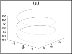
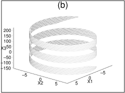
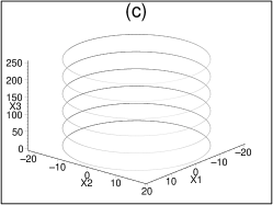
Figure 1: (a) A Kelvin wave at $\tau=0$, (b) and its motion during $-7<\tau<7$. (c) Smoke rings at $\tau=0,10,...,40,50$.

Figure 1 shows a Kelvin wave and a smoke ring configurations. Fig. 1-(a) is a Kelvin wave at $\tau=0$ and Fig. 1-(b) shows its motion during $-7<\tau<7$ moving along the z-axis. Fig. 1-(c) shows smoke rings at $\tau=0,10,...,40,50$. It shows that the surface swept out by a smoke ring is a cylinder. The straight line of Case A is thus a limiting case where the ring shrinks to a point.

4.3 Case C: Soliton

One of the well-known vortex configurations is the solitary kink wave which propagates along a straight vortex filament line. This was first found by Hasimoto [6] using the duality between the Da Rios-Betchov equation and the nonlinear Schrödinger equation. This Hasimoto soliton, which was obtained by dualizing the NLS soliton, has the form,

$${\bf X}=A\rm{sech}(\alpha\sigma-\beta\tau)\left(\cos(\gamma\sigma-\delta\tau),\ \sin(\gamma\sigma-\delta\tau),\ 0\right)+\left(0,\ 0,\ B\sigma-A\tanh(\alpha\sigma-\beta\tau)\right).$$ (65)

In the present case of the Lund-Regge model, a similar configuration can be found also by dualizing the soliton of the complex sine-Gordon equation as given in Case C. In order to do so, we first compute $\Phi$ by using the Bäcklund transformation in Eq. (31) applied to the vacuum ($f=1$) so that

$$\Phi={\lambda\over\lambda-i\delta/\sqrt{-\beta}}\Phi_{1}\Phi_{f},$$ (66)

where $\Phi_{f}$ is given in Eq. (34) and

$$\Phi_{1}=1+{\delta\over\sqrt{-\beta}\lambda}\pmatrix{-iu^{*}&\sqrt{1-uu^{*}}e^{i\theta}\cr-\sqrt{1-uu^{*}}e^{-i\theta}&iu},$$ (67)

with $u$ and $\theta$ as in Eq. (37). A straightforward calculation using Eq. (42) shows that

$$F_{1} = iR\sqrt{1-uu^{*}}\ \sin(2\beta\lambda z-{2\over\lambda}\bar{z}+\theta),$$

$$F_{2} = iR\sqrt{1-uu^{*}}\ \cos(2\beta\lambda z-{2\over\lambda}\bar{z}+\theta),$$

$$F_{3} = {iR\over 2}(u+u^{*})-i\lambda\beta z-{i\over\lambda}\bar{z},$$

$$R = {\sqrt{-\beta}\lambda\delta\over-\beta\lambda^{2}+\delta^{2}+2\sqrt{-\beta}\lambda\delta\sin{\alpha}}.$$ (68)

Using Eq. (50), we obtain the soliton solution,

$$X_{1} = {4R\over\beta}\cos{\alpha}\ \rm{sech}\Sigma\ \sin(-{\beta\over 2}\sigma+\theta),$$

$$X_{2} = {4R\over\beta}\cos{\alpha}\ \rm{sech}\Sigma\ \cos(-{\beta\over 2}\sigma+\theta),$$

$$X_{3} = -{4R\over\beta}\cos{\alpha}\ \tanh\Sigma-\tau,$$ (69)

where

$$\Sigma = {1\over 4}\sqrt{-\beta}\cos{\alpha}\Big{(}({\delta\over\lambda}-{\beta\lambda\over\delta})\tau+({\delta\over\lambda}+{\beta\lambda\over\delta})\sigma\Big{)},$$

$$\theta = {1\over 4}\sqrt{-\beta}\sin{\alpha}\Big{(}({\delta\over\lambda}+{\beta\lambda\over\delta})\tau+({\delta\over\lambda}-{\beta\lambda\over\delta})\sigma\Big{)},$$ (70)

which has the same form with the Hasimoto soliton in fluid dynamics.

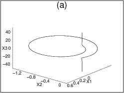
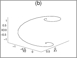
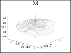
Figure 2: (a) A soliton vortex configuration at $\sigma=0$ and (b) an open string at $\tau=0$. (c) An embedded surface for $-20<\sigma<20$ and $-50<\tau<50$.

Figure 2 shows soliton vortex configurations with parameters $\alpha=0.8$, $\beta=-0.3$, $\delta=1.5$ and $\lambda=0.5$. Fig. 2-(a) is a Hasimoto-type vortex configuration where $\sigma=0$ and the curve is parametermized by $\tau$. Fig. 2-(b) is a open string configuration where $\tau=0$ and the curve is parametrized by $\sigma$, and Fig. 2-(c) is a surface swept out by a moving soliton vortex. We emphasize that due to the discrete symmetry of the vortex equation under the exchange $\sigma\leftrightarrow\tau$, the solution in Eq. (69) with $\sigma$ and $\tau$ exchanged is also a solution, thus roles of $\sigma$ and $\tau$ in the Figure 2 can also be exchanged.

4.4 Breather vortex

The breather solution of the sine-Gordon equation is presumably the most well-known configuration in soliton theories as a stable localized solution except solitons. Our dualization procedure suggests that we can also have a counterpart of a breather in vortex dynamics. As far as we know, such a configuration is not known in vortex dynamics literatures. In order to construct the solution explicitly, we use the BT in Eq. (31) to find $\Phi$ of the linear equation (26),

$$\Phi = (1+\Delta_{3}g_{3}^{-1}\bar{T}g_{1})(1+\Delta_{1}g_{1}^{-1}\bar{T})\Phi_{f}$$ (71)

$$= \left(1-i\sigma_{3}\Delta_{3}e^{i\sigma_{2}(\phi_{1}+\phi_{3})}\right)\left(1-i\sigma_{3}\Delta_{3}e^{i\sigma_{2}\phi_{1}}\right)\Phi_{f},$$

where $\Delta_{1}={\delta\over\lambda\sqrt{-\beta}}$, $\Delta_{3}={1\over\delta\lambda\sqrt{-\beta}}$ and $\phi_{1},\phi_{3}$ and $\Phi_{f}$ are given by Eq. (41) and (34). Using the definition $F\equiv\Phi^{-1}{\partial\over\partial t}\Phi$, we obtain

$$F_{1} = {i\Delta_{3}\over(1+\Delta_{1}^{2})(1+\Delta_{3}^{2})}\left(\Delta_{1}^{2}\sin(\phi_{1}-\phi_{3})\cos 2Y+\sin(\phi_{1}+\phi_{3})\cos 2Y-2\Delta_{1}\sin\phi_{3}\sin 2Y\right)$$

$$+ {i\Delta_{1}\over 1+\Delta_{1}^{2}}\sin\phi_{1}\cos 2Y,$$

$$F_{2} = {i\Delta_{3}\over(1+\Delta_{1}^{2})(1+\Delta_{3}^{2})}\left(-\Delta_{1}^{2}\sin(\phi_{1}-\phi_{3})\sin 2Y-\sin(\phi_{1}+\phi_{3})\sin 2Y-2\Delta_{1}\sin\phi_{3}\cos 2Y\right)$$

$$- {i\Delta_{1}\over 1+\Delta_{1}^{2}}\sin\phi_{1}\sin 2Y,$$

$$F_{3} = {i\Delta_{3}\over(1+\Delta_{1}^{2})(1+\Delta_{3}^{2})}\left(\Delta_{1}^{2}\cos(\phi_{1}-\phi_{3})+\cos(\phi_{1}+\phi_{3})\right)+{i\Delta_{1}\over 1+\Delta_{1}^{2}}\cos\phi_{1}-i\lambda\beta z-{i\bar{z}\over\lambda},$$ (72)

where $Y=\beta\lambda z-{\bar{z}\over\lambda}$. This gives a “breather vortex solution” after using the relation in Eq. (51). Figure 3 describes breather vortex configurations and the embedded surface. Fig. 3-(a) shows an open-string type breather vortex with $\tau=0$. Fig. 3-(b) a breather vortex configuration with $\sigma=0$, and Fig. 3-(c) shows an embedded surface. Note that Fig. 3-(a) shows a cusp at $\sigma=0$. However, this does not cause any physical singularity which may be seen by checking the derivatives of vortex coordinates with respect to $\sigma$ at $\sigma=0$. Explicit calculation shows that they behave regularly at $\sigma=0$. In fact, this cusp-like behavior arises since we have restricted to the breather of the sine-Gordon equation which arises as a special case of breather solutions of the complex sine-Gordon equation. Instead of proving this in terms of detailed solutions, here we only content that breather solutions obtained from solitons with $\alpha\neq 0$ do not possess this cusp-like behavior. Besides, we may expect that this new type vortex configuration is stable since it arises from dualizing a breather solution of the complex sine-Gordon equation which is stable. However, this has to yet to be seen.

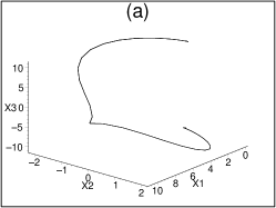
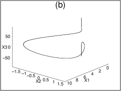
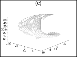
Figure 3: Breather vortex configurations with parameters $\lambda=0.5$, $\beta=-0.09$, $\delta=e^{0.5i}$, (a) an open-string configuration with $\tau=0$ and (b) a breather vortex with $\sigma=0$. (c) Embedded surface for $-100<\tau<100$ and $-60<\sigma<60$.

5 Discussion

In this paper, we have found various vortex configurations of the Lund-Regge model by making use of the duality between the Lund-Regge equation and the complex sine-Gordon equation. We have shown that these vortices have analogous counterparts in the vortex system of fluid dynamics. In fact, these correspondence arise from the fact that the usual fluid vortex equation is a “nonrelativistic limit” of the Lund-Regge equation. This may be also seen in their dualized versions, i.e. the nonlinear Schrödinger equation which dualizes the vortex equation in fluid dynamics also arises as a nonrelativistic limit of the sine-Gordon equation, which itself is a special case of the complex sine-Gordon equation. The exact correspondence of these equations will be considered elsewhere.

Another important problem would be the quantization of the system. In view of the string formulation of the system by Lund and Regge, the quantization of the present case would be a stringy generalization of the Landau levels of a charged particle moving on a uniform magnetic field. The magnetic flux vortex in the Maxwell Higgs system with a uniform magnetic field, for exampe, can be quantized consistently. It would be interesting to know whether the duality between the Lund-Regge model and the complex sine-Gordon model persists at the quantum level.

Acknowledgements

The work of K.Lee was supported in part by the SRC program of the SNU-CTP, the Basic Science and Research Program under BRSI-98-2418, and KOSEF 1998 Interdisciplinary Research Grant 98-07-02-07-01-5. Q-H. Park and H.J. Shin were supported in part by the program of Basic Science Research, Ministry of Education 1998-015-D00073, and by Korea Science and Engineering Foundation, 97-07-02-02-01-3. K. Lee acknowledge an useful discussion with Karen Uhlenbeck about the solutions of the chiral models, and K. Lee and Q-H. Park thank Aspen Center for Physics (1999 summer) where this work has been completed.

References

- [1] M. Kalb and P. Ramond, Phys. Rev. D9 (1974) 2273.
- [2] F. Lund and T. Regge, Phys. Rev. D14 (1976) 1524; F. Lund, Phys. Rev. Lett. 38 (1977) 1175.
- [3] A. Zee, Nucl. Phys. B421 (1994) 111.
- [4] see, for example, P.G. Saffman, Vortex dynamics, Cambridge University Press (1992), or R.J. Donnelly, Quantized vortices in helium II, Cambridge University Press (1991).
- [5] L.S. Da Rios, Sul Moto d’un liquido indefinito con un filetto vorticoso di forma qualunque, Rend. Circ. Mat. Palermo, 22 (1906) 117; R. Betchov, J. Fluid. Mech. 22 (1965) 471; R.L. Ricca, Nature, 352 (1991).
- [6] H. Hasimoto, J. Fluid Mech. 51 (1972 ) 477; E.J. Hopfiner, F.K. Browand and Y. Gagne, J. Fluid Mech. 125 (1982) 505; T. Maxworthy, E.J. Hopfinger and L.G. Redekopp, J. Fluid. Mech. 151 (1985) 141.
- [7] D.C. Samuels and R.J. Donnelly, Phys. Rev. Lett. 61 (1990) 1385.
- [8] see for example, Y. Yasui and N. Sasaki, Differential geometry of the vortex filament equation, hep-th/9611073.
- [9] Q-H. Park and H.J. Shin, Phys. Lett. B454 (1999) 259.
- [10] R.L. Davis and E.P.S. Shellard, Phys. Rev. Lett 63, 2029 (1989); U. Ben-Ya’acov, Nucl. Phys. B382, 592 (1992); K. Lee, Phys. Rev. D48, 2493 (1993).
- [11] F. Lund, Ann. of Phys. (New York) 115 (1978) 251.
- [12] K. Pohlmeyer, Commun. Math. Phys. 46 (1976) 207.
- [13] C.R. Nappi, Phys. Rev. D21 (1980) 418.
- [14] V.E. Zakharov and A.V. Mikhailov, Sov. Phys. JETP 47(6), 161 (1987).
- [15] T. Curtright and C. Zachos, Phys. Rev. D49 (1994) 5408.
- [16] K. Uhlenbeck, J. Diff. Geom. 30, (1989) 1; J. Geom. Phys. 8, (1992) 283.
- [17] I. Bakas, Int. J. Mod. Phys. A9 (1994) 3443.
- [18] Q-H. Park, Phys. Lett. B328 (1994) 329; Q-H. Park and H.J. Shin, Phys. Lett. B347 (1995) 73.
- [19] D.Karabali, Q-H.Park, H.J.Schnitzer and Z.Yang, Phys. Lett. B216, (1989) 307; K.Gawedski and A.Kupiainen,, Nucl. Phys. B320, (1989) 625.
- [20] N. Dorey and T.J. Hollowood, Nucl. Phys. B440 (1995) 215.
- [21] Q-H. Park and H.J. Shin, Phys. Lett. B359 (1995) 125.
- [22] I. Bakas, Q-H. Park and H.J. Shin, Phys. Lett. B372 (1996) 45.