Abstract

This is a contracted version of a series of lectures for graduate and undergraduate students given at the “VI Seminario Nazionale di Fisica Teorica” (Parma, September 1997), at the Second Int. Conference “Around VIRGO” (Pisa, September 1998), and at the Second SIGRAV School on “Gravitational Waves in Astrophysics, Cosmology and String Theory” (Center “A. Volta”, Como, April 1999). The aim is to provide an elementary, self-contained introduction to string cosmology and, in particular, to the background of relic cosmic gravitons predicted in the context of the so-called “pre-big bang” scenario. No special preparation is required besides a basic knowledge of general relativity and of standard (inflationary) cosmology. All the essential computations are reported in full details either in the main text or in the Appendices. For a deeper and more complete approach to the pre-big bang scenario the interested reader is referred to the updated collection of papers available at http://www.to.infn.it/~gasperin/.

[Pre-big bang cosmology]Elementary introduction to pre-big bang cosmology and to the relic graviton background

M. Gasperini†‡

Preprint BA-TH/99-345              E-print Archives: hep-th/9907067

1 Introduction

The purpose of these lectures is to provide an introduction to the background of relic gravitational waves expected in a string cosmology context, and to discuss its main properties. To this purpose, it seems to be appropriate to include a short presentation of string cosmology, in order to explain the basic ideas underlying the so-called pre-big bang scenario, which is one of the most promising scenarios for the production of a detectable graviton background of cosmological origin.

After a short, qualitative presentation of the pre-big bang models, I will concentrate on the details of the cosmic graviton spectrum: I will discuss the theoretical predictions for different models, and I will compare the predictions with existing phenomenological constraints, and with the expected sensitivities of the present gravity wave detectors. A consistent part of these lectures will thus be devoted to introduce the basic notions of cosmological perturbation theory, which are required to compute the graviton spectrum and to understand why the amplification of tensor metric perturbations, at high frequency, is more efficient in string cosmology than in the standard inflationary context.

Let me start by noting that a qualitative, but effective representation of the main difference between string cosmology and standard, inflationary cosmology can be obtained by plotting the curvature scale of the Universe versus time, as illustrated in Fig. 1.

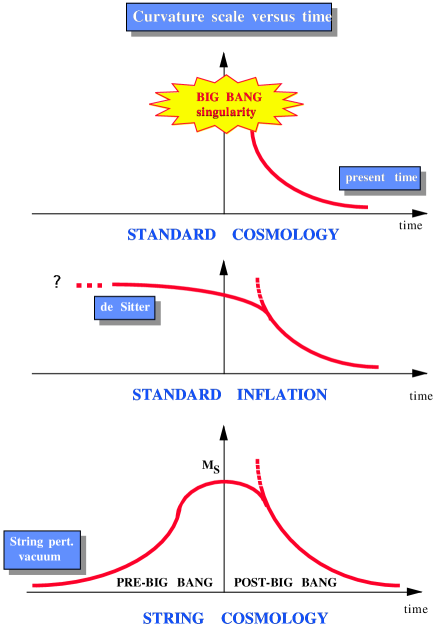
Figure 1: Time evolution of the curvature scale in the standard cosmological scenario, in the conventional inflationary scenario, and in the string cosmology scenario.

According to the cosmological solutions of the so-called “standard” scenario [3], the spacetime curvature decreases in time. As we go back intime the curvature grows monotonically, and blows up at the initial “big bang” singularity, as illustrated in the top part of Fig. 1 (a similar plot, in the standard scenario, also describes the behaviour of the temperature and of the energy density of the gravitational sources).

According to the standard inflationary scenario [4], on the contrary, the Universe in the past is expected to enter a de Sitter, or “almost” de Sitter phase, during which the curvature tends to stay frozen at a nearly constant value. From a classical point of view, however, this scenario has a problem, since a phase of expansion at constant curvature cannot be extended back in time for ever [5], for reasons of geodesic completeness. This point was clearly stressed also in Alan Guth’s recent survey of inflationary cosmology [6]:

“… Nevertheless, since inflation appears to be eternal only into the future, but not to the past, an important question remains open. How did all start? Although eternal inflation pushes this question far into the past, and well beyond the range of observational tests, the question does not disappear.”

A possible anwer to this question, in a quantum cosmology context, is that the Universe emerges in a de Sitter state “from nothing” [7] (or from some unspecified “vacuum”), though a process of quantum tunnelling. I will not discuss the quantum approach in these lectures, but let me note that the computation of the transition probability requires an appropriate choice of the boundary conditions [8], which in the context of standard inflation are imposed “ad hoc” when the Universe is in an unknown state, deeply inside the non-perturbative, quantum gravity regime. In a string cosmology context, on the contrary, the initial conditions are referrred asymptotically to a low-energy, classical state which is known, and well controlled by the low-energy string effective action [9].

From a classical point of view, however, the answer to the above question – what happens to the Universe before the phase of constant curvature, which cannot last for ever – is very simple, as we are left only with two possibilities. Either the curvature starts growing again, at some point in the past (but in this case the singularity problems remains, it is simply shifted back in time), or the curvature starts decreasing.

In this second case we are just led to the string cosmology scenario, illustrated in the bottom part of Fig. 1. String theory suggests indeed for the curvature a specular behaviour (or better a “dual” behaviour, as we shall see in a moment) around the time axis. As we go back in time the curvature grows, reaches a maximum controlled by the string scale, and then decreases towards a state which is asymptotically flat and with negligible interactions (vanishing coupling constants), the so-called “string perturbative vacuum”. In this scenario the phase of high, but finite (nearly Planckian) curvature is what replaces the big bang singularity of the standard scenario. It comes thus natural, in a string cosmology context, to call “pre-big bang” [10] the initial phase with growing curvature, in contrast to the subsequent, standard, “post-big bang ” phase with decreasing curvature.

At this point, a number of questions may arise naturally. In particular:

• Motivations: why such a cosmological scenario, characterized by a “bell-like” shape of the curvature, seems to emerge in a string cosmology context and not, for istance, in the context of standard cosmology based on the Einstein equations?

• Kinematics: in spite of the differences, is the kinematic of the pre-big bang phase still appropriate to solve the well known problems (horizon, flatness …) of the standard scenario? After all, we do not want to loose the main achievements of the conventional inflationary models.

• Phenomenology: are there phenomenological consequence that can discriminate between string cosmology models and other inflationary models? and are such effects observable, at least in principle?

In the following sections I will present a quick discussion of the three points listed above.

2 Motivations: duality symmetry

There are various motivations, in the context of string theory, suggesting a cosmological scenario like that illustrated in Fig. 1. All the motivations are however related, more or less directly, to an important property of string theory, the duality symmetry of the effective action.

To illustrate this point, let me start by recalling that in general relativity the solutions of the standard Einstein action,

$$S=-{1\over 2\lambda_{p}^{d-1}}\int d^{d+1}x\sqrt{|g|}~{}R$$ (2.1)

($d$ is the number of spatial dimensions, and $\lambda_{p}=M_{p}^{-1}$ is the Planck length scale), are invariant under “time-reversal” transformations. Consider, for instance, a homogeneous and isotropic solution of the cosmological equations, represented by a scale factor $a(t)$:

$$ds^{2}=dt^{2}-a^{2}(t)dx_{i}^{2}.$$ (2.2)

If $a(t)$ is a solution, then also $a(-t)$ is a solution. On the other hand, when $t$ goes into $-t$, the Hubble parameter $H=\dot{a}/a$ changes sign,

$$a(t)\rightarrow a(-t),~{}~{}~{}~{}~{}~{}~{}~{}~{}~{}~{}~{}~{}~{}~{}~{}H=\dot{a}/a\rightarrow-H.$$ (2.3)

To any standard cosmological solution $H(t)$, describing decelerated expansion and decreasing curvature ($H>0$, $\dot{H}<0$), is thus associated a “reflected” solution, $H(-t)$, describing a contracting Universe because $H$ is negative.

This is the situation in general relativity. In string theory the action, in addition to the metric, contains at least another fundamental field, the scalar dilaton $\phi$. At the tree-level, namely to lowest order in the string coupling and in the higher-derivatives ($\alpha^{\prime}$) string corrections, the effective action which guarantees the absence of conformal anomalies for the motion of strings in curved backgrounds (see the Apppendix A) can be written as:

$$S=-{1\over 2\lambda_{s}^{d-1}}\int d^{d+1}x\sqrt{|g|}~{}e^{-\phi}\left[R+\left(\partial_{\mu}\phi\right)^{2}\right]$$ (2.4)

( $\lambda_{s}=M_{s}^{-1}$ is the fundamental string length scale; see the Appendix B for notations and sign conventions). In addition to the invariance under time-reversal, the above action is also invariant under the “dual” inversion of the scale factor, accompanied by an appropriate transformation of the dilaton (see [11] and the first paper of Ref. [10]). More precisely, if $a(t)$ is a solution for the cosmological background (2.2) , then $a^{-1}(t)$ is also a solution, provided the dilaton transforms as:

$$a\rightarrow\tilde{a}=a^{-1},~{}~{}~{}~{}~{}~{}~{}~{}~{}~{}~{}~{}~{}~{}~{}~{}\phi\rightarrow\tilde{\phi}=\phi-2d\ln a$$ (2.5)

(this transformation implements a particular case of $T$-duality symmetry, usually called “scale factor duality”, see the Appendix B).

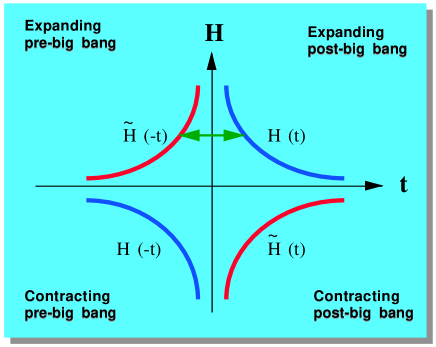
Figure 2: The four branches of a low-energy string cosmology background.

When $a$ goes into $a^{-1}$, the Hubble parameter $H$ again goes into $-H$ so that, to each one of the two solutions related by time reversal, $H(t)$ and $H(-t)$, is associated a dual solution, $\tilde{H}(t)$ and $\tilde{H}(-t)$, respectively (see Fig. 2). The space of solutions is thus reacher in a string cosmology context. Indeed, because of the combined invariance under the transformations (2.3) and (2.5), a cosmological solution has in general four branches: two branches describe expansion (positive $H$), two branches describe contraction (negative $H$). Also, as illustrated in Fig. 2, for two branches the curvature scale ($\sim H^{2}$) grows in time, with a typical “pre-big bang” behaviour, while for the other two branches the curvature scale decreases, with a typical “post-big bang” behaviour.

It follows, in this context, that to any given decelerated expanding solution, $H(t)>0$, with decreasing curvature, $\dot{H}(t)<0$ (typical of the standard cosmological scenario), is always associated a “dual partner” describing accelerated expansion, $\tilde{H}(-t)>0$, and growing curvature, $\dot{\tilde{H}}(-t)>0$. This doubling of solutions has no analogue in the context of the Einstein cosmology, where there is no dilaton, and the duality symmetry cannot be implemented.

It should be stressed, before proceeding further, that the duality symmetry is not restricted to the case of homogeneous and isotropic backgrounds like (2.2), but is expected to be a general property of the solutions of the string effective action (possibly valid at all orders [12], with the appropriate generalizations). The inversion of the scale factor, in particular, and the associated transformation (2.5), is only a special case of a more general, $O(d,d)$ symmetry of the string effective action, which is manifest already at the lowest order. In fact, the tree-level action in general contains, besides the metric and the dilaton, also a second rank antisymmetric tensor $B_{\mu\nu}$, the so-called Kalb-Ramond “universal” axion:

$$S=-{1\over 2\lambda_{s}^{d-1}}\int d^{d+1}x\sqrt{|g|}~{}e^{-\phi}\left[R+\left(\partial_{\mu}\phi\right)^{2}-{1\over 12}\left(\partial_{[\mu}B_{\nu\alpha]}\right)^{2}\right].$$ (2.6)

Given a background, even anisotropic, but with $d$ abelian isometries, this action is invariant under a global, pseudo-orthogonal group of $O(d,d)$ transformations which mix in a non-trivial way the components of the metric and of the antisymmetric tensor, leaving invariant the so-called “shifted” dilaton $\overline{\phi}$:

$$\overline{\phi}=\phi-\ln\sqrt{|{\rm det}g_{ij}|}.$$ (2.7)

In the particular, “cosmological” case in which we are interested in, the $d$ isometries correspond to spatial traslations (namely, we are in the case of a homogeneous, Bianchi I type metric background). For this background, the action (2.6) can be rewritten in terms of the $2d\times 2d$ symmetric matrix $M$, defined by the spatial components of the metric, $g_{ij}$, and of the axion, $B_{ij}$, as:

$$B\equiv B_{ij},~{}~{}~{}~{}~{}~{}~{}G\equiv g_{ij},~{}~{}~{}~{}~{}~{}~{}M=\pmatrix{G^{-1}&-G^{-1}B\cr BG^{-1}&G-BG^{-1}B\cr}.$$ (2.8)

In the cosmic time gauge, the action takes the form (see the Appendix B)

$$S=-{\lambda_{s}\over 2}\int dt~{}e^{-\overline{\phi}}\left[(\dot{\overline{\phi}})^{2}+{1\over 8}{\rm Tr}~{}\dot{M}(M^{-1})\dot{}~{}\right],$$ (2.9)

and is manifestly invariant under the set of global transformations [13]:

$$\overline{\phi}\rightarrow\overline{\phi},~{}~{}~{}~{}~{}~{}~{}~{}M\rightarrow\Lambda^{T}M\Lambda,~{}~{}~{}~{}~{}~{}~{}~{}\Lambda^{T}\eta\Lambda=\eta,~{}~{}~{}~{}~{}~{}~{}~{}\eta=\pmatrix{0&I\cr I&0\cr},$$ (2.10)

where $I$ is the d-dimensional unit matrix, and $\eta$ is the $O(d,d)$ metric in off-diagonal form. The transformation (2.5), representing scale factor duality, is now reproduced as a particular case of (2.10) with the trivial $O(d,d)$ matrix $\Lambda=\eta$, and for an isotropic background with $B_{\mu\nu}=0$.

This $O(d,d)$ symmetry holds even in the presence of matter sources, provided they transform according to the string equations of motion in the given background [14]. In the perfect fluid approximation, for instance, the inversion of the scale factor corresponds to a reflection of the equation of state, which preserves however the “shifted” energy $\overline{\rho}=\rho|{\rm det}g_{ij}|^{1/2}$:

$$a\rightarrow\tilde{a}=a^{-1},~{}~{}~{}~{}~{}~{}~{}~{}\overline{\phi}\rightarrow\overline{\phi},~{}~{}~{}~{}~{}~{}~{}~{}p/\rho\rightarrow-p/\rho,~{}~{}~{}~{}~{}~{}~{}~{}\overline{\rho}\rightarrow\overline{\rho}$$ (2.11)

A detailed discussion of the duality symmetry is outside the purpose of these lectures. What is important, in our context, is the simultaneous presence of duality and time-reversal symmetry: by combining these two symmetries, in fact, it is possible in principle to obtain cosmological solutions of the “self-dual” type, characterized by the conditions

$$a(t)=a^{-1}(-t),~{}~{}~{}~{}~{}~{}~{}~{}~{}~{}~{}~{}~{}~{}~{}~{}\overline{\phi}(t)=\overline{\phi}(-t).$$ (2.12)

They are important, as they connect in a smooth way the phase of growing and decreasing curvature, and also describe a smooth evolution from the string perturbative vacuum (i.e. the asymptotic no-interaction state in which $\phi\rightarrow-\infty$ and the string coupling is vanishing, $g_{s}=\exp(\phi/2)\rightarrow 0$), to the present cosmological phase in which the dilaton is frozen, with an expectation value [15] $\langle g_{s}\rangle=M_{s}/M_{p}\sim 0.3$ – $0.03$ (see Fig. 3).

The explicit occurrence of self-dual solutions and, more generally, of solutions describing a complete and smooth transition between the phase of pre- and post-big bang evolution, seems to require in general the presence of higher order (higher loop and/or higher derivative) corrections to the string effective action [16] (see however [17, 18]). So, in order to give only a simple example of combined $\{$duality $\bigoplus$ time-reversal$\}$ transformation, let me consider here the low-energy, asymptotic regimes, which are well described by the lowest order effective action.

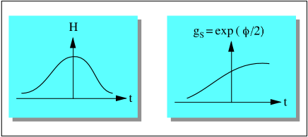
Figure 3: Time evolution of the curvature scale $H$ and of the string coupling $g_{s}=\exp(\phi/2)\simeq M_{s}/M_{p}$, for a typical self-dual solution of the string cosmology equations.

By adding matter sources, in the perfect fluid form, to the action (2.4), the string cosmology equations for a $d=3$, homogeneous, isotropic and conformally flat background can be written as (see Appendix C, eqs. (3.16), (3.18), (3.15), respectively):

$$\dot{\phi}^{2}-6H\dot{\phi}+6H^{2}=e^{\phi}\rho,$$

$$\dot{H}-H\dot{\phi}+3H^{2}={1\over 2}e^{\phi}p,$$

$$2\ddot{\phi}+6H\dot{\phi}-\dot{\phi}^{2}-6\dot{H}-12H^{2}=0.$$ (2.13)

For $p=\rho/3$, in particular, they are exactly solved by the standard solution with constant dilaton (see eqs. (3.32), (3.33)),

$$a\sim t^{1/2},~{}~{}~{}~{}~{}~{}~{}~{}~{}\rho=3p\sim a^{-4},~{}~{}~{}~{}~{}~{}~{}~{}~{}\phi={\rm const},~{}~{}~{}~{}~{}~{}~{}~{}~{}t\rightarrow+\infty,$$ (2.14)

describing decelerated expansion and decreasing curvature scale:

$$\dot{a}>0,~{}~{}~{}~{}~{}~{}~{}~{}~{}\ddot{a}<0,~{}~{}~{}~{}~{}~{}~{}~{}~{}\dot{H}<0.$$ (2.15)

This is exactly the radiation-dominated solution of the standard cosmological scenario, based on the Einstein equations. In string cosmology, however, to this solution is associated a “dual complement”, i.e. an additional solution which can be obtained by applying on the background (2.14) a time-reversal transformation $t\rightarrow-t$, and the duality transformation (2.11):

$$a\sim(-t)^{-1/2},~{}~{}~{}~{}~{}\phi\sim-3\ln(-t),~{}~{}~{}~{}~{}\rho=-3p\sim a^{-2},~{}~{}~{}~{}~{}t\rightarrow-\infty,$$ (2.16)

This is still an exact solution of the equations (2.13) (see the Appendix C), describing however accelerated (i.e. inflationary) expansion, with growing dilaton and growing curvature scale:

$$\dot{a}>0,~{}~{}~{}~{}~{}~{}~{}~{}~{}\ddot{a}>0,~{}~{}~{}~{}~{}~{}~{}~{}~{}\dot{H}>0.$$ (2.17)

We note, for future reference, that accelerated expansion with growing curvature is usually called “superinflation” [19], or “pole-inflation”, to distinguish it from the more conventional power-inflation, with decreasing curvature.

The two solutions (2.14) and (2.16) provide a particular, explicit representation of the scenario illustrated in Fig. 3, in the two asympotic regimes of $t$ large and positive, and $t$ large and negative, respectively. The duality symmetry seems thus to provide an important motivation for the pre-big bang scenario, as it leads naturally to introduce a phase of growing curvature, and is a crucial ingredient for the “bell-like” scenario of Fig. 3.

It should be noted that pure scale factor duality, by itself, is not enough to convert a phase of decreasing into growing curvature (see for instance Fig. 2, where it is clearly shown that $H$ and $\tilde{H}$, in the same temporal range, lead to the same evolution of the curvature scale, $H^{2}\sim\tilde{H}^{2}$). Time reflection is thus necessarily required, if we want to invert the curvature behaviour. From this point of view, time-reversal symmetry is more important than duality.

In a thermodynamic context, however, duality by itself is able to suggests the existence of a primordial cosmological phase with “specular” properties with respect to the present, standard cosmological phase [20]. It must be stressed, in addition, that it is typically in the cosmology of extended objects that the phase of growing curvature may describe accelerated expansion instead of contraction, and that the growth of the curvature may be regularized, instead of blowing up to a singularity. For instance, it is with the string dilaton [10], or with a network of strings self-consistently coupled to the background [21], that we are naturally lead to superinflation. Also, in quantum theories of extended objects, it is the minimal, fundamental lenght scale of the theory that is expected to bound the curvature, and to drive superinflation to a phase of constant, limiting curvature [22] asymptotically approaching de Sitter, as explicitly checked in a string theory context [23]. Duality symmetries, on the other hand, are typical of extended objects (and of strings, in particular), so that it is certainly justified to think of duality as of a fundamental motivation and ingredient of the pre-big bang scenario.

Duality is an important symmetry of modern theoretical physics, and to conclude this section I would like to present an analogy with another very important symmetry, namely supersymmetry (see Table I).

	SUPERSYMMETRY	DUALITY + TIME-REVERSAL
Pair of partners	{bosons, fermions}	{growing curvature, decreasing curvature}
Known states	photons, gravitons, …	decelerated, standard  post-big bang
Predicted	photinos, gravitinos, …	accelerated, inflationary  pre-big bang

Table 1: Analogy between supersymmetry and duality.

According to supersymmetry, to any bosonic state is associated a fermionic partner, and viceversa. From the existence of bosons that we know to be present in Nature, if we believe in supersymmetry, we can predict the existence of fermions not yet observed, like the photino, the gravitino, and so on.

In the same way, according to duality and time-reversal, to any geometrical state with decreasing curvature is associated a dual partner with growing curvature. On the other hand, our Universe, at present, is in the standard post-big bang phase, with decreasing curvature. If we believe that duality has to be implemented, even approximately, in the course of the cosmological evolution, we can then predict the existence of a phase, in the past, characterized by growing curvature and by a typical pre-big bang evolution.

3 Kinematics: shrinking horizons

If we accept, at least as a working hypothesis, the possibility that our Universe had in the past a “dual” complement, with growing curvature, we are lead to the second of the three questions listed in Section 1: is the kinematics of the pre-big bang phase still appropriate to solve the problems of the standard inflationary scenario? The anwer is positive, but in a non-trival way.

Consider, for instance, the present cosmological phase. Today the dilaton is expected to be constant, and the Universe should be appropriately described by the Einstein equations. The gravitational part of such equations contains two types of terms: terms controlling the geometric curvature of a space-like section, evolving in time like $a^{-2}$, and terms controlling the gravitational kinetic energy, i.e. the spacetime curvature scale, evolving like $H^{2}$. According to present observations the spatial curvature term is non-dominant, i.e.

$$r={a^{-2}\over H^{2}}\sim{\rm spatial~{}curvature\over spacetime~{}curvature}~{}\raise 1.72218pt\hbox{$<$}\kern-8.00003pt\lower 2.6694pt\hbox{$\sim$}~{}1.$$ (3.1)

According to the standard cosmological solutions, on the other hand, the above ratio must grow in time. In fact, by putting $a\sim t^{\beta}$,

$$r\sim\dot{a}^{-2}\sim t^{2(1-\beta)},$$ (3.2)

so that $r$ keeps growing both in the matter-dominated ($\beta=2/3$) and in the radiation-dominated ($\beta=1/2$) era. Thus, as we go back in time, $r$ becomes smaller and smaller, and when we set initial conditions (for instance, at the Planck scale) we have to impose an enormous fine tuning of the spatial curvature term, with respect to the other terms of the cosmological equations. This is the so-called flatness problem.

The problem can be solved if we introduce in the past a phase (usually called inflation), during which the value of $r$ was decreasing, for a time long enough to compensate the subsequent growth during the phase of standard evolution. It is important to stress that this requirement, in general, can be implemented by two physically different classes of backgrounds.

Consider for simplicity a power-law evolution of the scale factor in cosmic time, with a power $\beta$, so that the time-dependence of $r$ is the one given in eq. (3.2). The two possible classes of backgrounds corresponding to a decreasing $r$ are then the following:

• Class I: $a\sim t^{\beta},\beta>1,t\rightarrow+\infty$. This class of backgrounds corresponds to what is conventionally called “power inflation”, describing a phase of accelerated expansion and decreasing curvature scale, $\dot{a}>0,\ddot{a}>0,\dot{H}<0$. This class contains, as a limiting case, the standard de Sitter inflation, $\beta\rightarrow\infty$, $a\sim e^{Ht}$, $\dot{H}=0$, i.e. accelerated exponential expansion at constant curvature.

• Class II: $a\sim(-t)^{\beta},\beta<1,t\rightarrow 0_{-}$. This is the class of backgrounds corresponding to the string cosmology scenario. There are two possible subclasess:

  • : $\beta<0$, describing superinflation, i.e. accelerated expansion with growing curvature scale, $\dot{a}>0,\ddot{a}>0,\dot{H}>0$;

  • : $0<\beta<1$, describing accelerated contraction and growing curvature scale, $\dot{a}<0,\ddot{a}<0,\dot{H}<0$.

A phase of growing curvature, if accelerated like in the pre-big bang scenario, can thus provide an unconventional, but acceptable, inflationary solution of the flatness problem (the same is true for the other standard kinematical problems, see [10]). It is important to stress, in particular, that the two subclasses IIa, IIb, do not correspond to different models, as they are simply different kinematical representation of the same scenario in two different frames, the string frame (S-frame), in which the effective action takes the form (2.4),

$$S(g,\phi)=-\int d^{d+1}x\sqrt{|g|}~{}e^{-\phi}\left[R+g^{\mu\nu}\partial_{\mu}\phi\partial_{\nu}\phi\right],$$ (3.3)

and the Einstein frame (E-frame), in which the dilaton is minimally coupled to the metric, and has a canonical kinetic term:

$$S(\tilde{g},\tilde{\phi})=-\int d^{d+1}x\sqrt{|\tilde{g}|}~{}\left[\tilde{R}-{1\over 2}\tilde{g}^{\mu\nu}\partial_{\mu}\tilde{\phi}\partial_{\nu}\tilde{\phi}\right].$$ (3.4)

In order to illustrate this point, we shall proceed in two steps. First we will show that, through a field redefinition $g=g(\tilde{g},\tilde{\phi})$, $\phi=\phi(\tilde{g},\tilde{\phi}),$, it is always possible to move from the S-frame to the E-frame; second, we will show that, by applying such a redefinition, a superinflationary solution obtained in the S-frame becomes an accelerated contraction in the E-frame, and viceversa.

We shall consider, for simplicity, an isotropic, spatially flat background with $d$ spatial dimensions, and we set:

$$g_{\mu\nu}={\rm diag}\left(N^{2},-a^{2}\delta_{ij}\right),~{}~{}~{}~{}~{}~{}~{}\phi=\phi(t),$$ (3.5)

where $g_{00}=N^{2}$ is to be fixed by an arbitrary choice of gauge. For this background we get:

$$\Gamma_{0i}\,^{j}=H\delta_{i}^{j},~{}~{}~{}~{}~{}~{}~{}\Gamma_{ij}\,^{0}={a\dot{a}\over N^{2}}\delta_{ij},~{}~{}~{}~{}~{}~{}~{}\Gamma_{00}^{0}={\dot{N}\over N}=F$$

$$R={1\over N^{2}}\left[2dFH-2d\dot{H}-d(d+1)H^{2}\right],$$ (3.6)

and the S-frame action (3.3) becomes

$$S(g,\phi)=-\int d^{d+1}x{a^{d}e^{-\phi}\over N}\left[2dFH-2d\dot{H}-d(d+1)H^{2}+\dot{\phi}^{2}\right]$$ (3.7)

Modulo a total derivative, we can eliminate the first two terms, and the action takes the quadratic form

$$S(g,\phi)=-\int d^{d+1}x{a^{d}e^{-\phi}\over N}\left[\dot{\phi}^{2}-2dH\dot{\phi}+d(d-1)H^{2}\right]$$ (3.8)

where, as expected, $N$ plays the role of a Lagrange multiplier (no kinetic term in the action).

In the E-frame the variables are $\tilde{N},\tilde{a},\tilde{\phi}$, and the action(3.4), after integration by part, takes the canonical form

$$S(\tilde{g},\tilde{\phi})=-\int d^{d+1}x{\tilde{a}^{d}\over\tilde{N}}\left[-{1\over 2}\dot{\tilde{\phi}}^{2}+d(d-1)H^{2}\right]$$ (3.9)

A quich comparison with eq. (3.8) leads finally to the field redefinition (no coordinate transformation!) connecting the Einstein and String frame:

$$\tilde{a}=ae^{-\phi/(d-1)},~{}~{}~{}~{}~{}~{}~{}~{}~{}\tilde{N}=Ne^{-\phi/(d-1)},~{}~{}~{}~{}~{}~{}~{}~{}~{}\tilde{\phi}=\phi\sqrt{2\over d-1}.$$ (3.10)

In fact, the above transformation gives

$$\tilde{H}=H-{\dot{\phi}\over d-1}$$ (3.11)

and, when inserted into eq. (3.9), exactly reproduces the S-frame action (3.8).

Consider now a superinflationary, pre-big bang solution obtained in the S-frame, for instance the isotropic, $d$-dimensional vacuum solution

$$a=(-t)^{-1/\sqrt{d}},~{}~{}~{}~{}~{}~{}~{}~{}~{}e^{\phi}=(-t)^{-(\sqrt{d}+1)},~{}~{}~{}~{}~{}~{}~{}~{}~{}t<0,~{}~{}~{}~{}~{}~{}~{}~{}~{}~{}t\rightarrow 0_{-}$$ (3.12)

(aee Appendix B, eqs. (2.21), (2.22)), and look for the corresponding E-frame solution. The above solution is valid in the syncronous gauge, $N=1$, and if we choose, for instance, the syncronous gauge also in the E-frame, we can fix $\tilde{N}$ by the condition:

$$\tilde{N}dt\equiv Ne^{-\phi/(d-1)}dt=d\tilde{t},$$ (3.13)

which defines the E-frame cosmic time, $\tilde{t}$, as:

$$d\tilde{t}=e^{-\phi/(d-1)}dt.$$ (3.14)

After integration

$$t\sim\tilde{t}^{d-1\over d+\sqrt{d}},$$ (3.15)

and the transformed solution takes the form:

$$\tilde{a}=(-\tilde{t})^{1/{d}},~{}~{}~{}~{}~{}~{}~{}~{}~{}e^{\tilde{\phi}}=(-\tilde{t})^{-\sqrt{2(d-1)\over d}},~{}~{}~{}~{}~{}~{}~{}~{}~{}\tilde{t}<0,~{}~{}~{}~{}~{}~{}~{}~{}~{}\tilde{t}\rightarrow 0_{-}.$$ (3.16)

One can easily check that this solution describes accelerated contraction with growing dilaton and growing curvature scale:

$${d\tilde{a}\over d\tilde{t}}<0,~{}~{}~{}~{}~{}~{}~{}{d^{2}\tilde{a}\over d\tilde{t}^{2}}<0,~{}~{}~{}~{}~{}~{}~{}{d\tilde{H}\over d\tilde{t}}<0,~{}~{}~{}~{}~{}~{}~{}{d\tilde{\phi}\over d\tilde{t}}>0.$$ (3.17)

The same result applies if we transform other isotropic solutions from the String to the Einstein frame, for instance the perfect fluid solution of Appendix C, eq. (3.32). We leave this simple exercise to the interested reader.

Having discussed the “dynamical” equivalence (in spite of the kinematical differences) of the two classes of string cosmology metrics, IIa and IIb, it seems appropriate at this point to stress the main dynamical difference between standard inflation, Class I metrics, and pre-big bang inflation, Class II metrics. Such a difference can be conveniently illustrated in terms of the proper size of the event horizon, relative to a given comoving observer.

Consider in fact the the proper distance, $d_{e}(t)$, between the surface of the event horizon and a comoving observer, at rest at the origin of an isotropic, conformally flat background [24]:

$$d_{e}(t)=a(t)\int_{t}^{t_{M}}dt^{\prime}a^{-1}(t^{\prime}),$$ (3.18)

Here $t_{M}$ is the maximal allowed extension, towards the future, of the cosmic time coordinate for the given background manifold. The above integral coverges for all the above classes of accelerated (expanding or contracting) scale factors. In the case of Class I metrics we have, in particular,

$$d_{e}(t)=t^{\beta}\int_{t}^{\infty}dt^{\prime}t^{\prime-\beta}={t\over\beta-1}\sim H^{-1}(t)$$ (3.19)

for power-law inflation ($\beta>1,t>0$), and

$$d_{e}(t)=e^{Ht}\int_{t}^{\infty}dt^{\prime}e^{-Ht^{\prime}}=H^{-1}$$ (3.20)

for de Sitter inflation. For Class II metrics ($\beta<1,t<0$) we have instead

$$d_{e}(t)=(-t)^{\beta}\int_{t}^{0}dt^{\prime}(-t^{\prime})^{-\beta}={(-t)\over 1-\beta}\sim H^{-1}(t).$$ (3.21)

In all cases the proper size $d_{e}(t)$ evolves in time like the so-called Hubble horizon (i.e. the inverse of the Hubble parameter), and then like the inverse of the curvature scale. The size of the horizon is thus constant or growing in standard inflation (Class I), decreasing in pre-big bang inflation (Class II), both in the S-frame and in the E-frame.

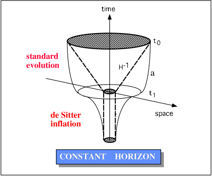
Figure 4: Qualitative evolution of the Hubble horizon (dashed curve) and of the scale factor (full curve) in the standard inflationary scenario.

Such an important difference is clearly illustrated in Fig. 4 and Fig. 5, where the dashed lines represent the evolution of the horizon, the full lines the evolution of the scale factor. The shaded area at time $t_{0}$ represents the portion of Universe inside our present Hubble radius. As we go back in time, according to the standard scenario, the horizon shrinks linearly, ($H^{-1}\sim t$), but the decrease of the scale factor is slower so that, at the beginning of the phase of standard evolution ($t=t_{1}$), we end up with a causal horizon much smaller than the portion of Universe that we presently observe. This is the well known “horizon problem” of the standard scenario.

In Fig. 4 the phase of standard evolution is preceeded in time by a phase of standard de Sitter inflation. Going back in time, for $t<t_{1}$, the scale factor keeps shrinking, and our portion of Universe “re-enters” inside the Hubble radius during a phase of constant (or slightly growing in time) horizon.

In Fig. 5 the standard evolution is preceeded in time by a phase of pre-big bang inflation, with growing curvature . The Universe “re-enters” the Hubble radius during a phase of shrinking horizon. To emphasize the difference, I have plotted the evolution of the scale factor both in the expanding S-frame, $a(t)$, and in the contracting E-frame, $\tilde{a}(t)$. Unlike in standard inflation, the proper size of the initial portion of the Universe may be very large in strings (or Planck) units, but not larger than the initial horizon itself [25], as emphasized in the picture. The initial horizon is large because the initial curvature scale is small, in string units, $H_{i}\ll 1/\lambda_{s}$.

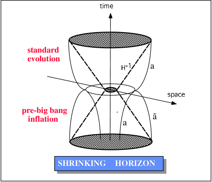
Figure 5: Qualitative evolution of the Hubble horizon (dashed curve) and of the scale factor (full curve) in the pre-big bang inflationary scenario, in the S-frame, $a(t)$, and in the E-frame, $\tilde{a}(t)$.

This is a basic consequence of the choice of the initial state which, in the pre-big bang scenario, approaches the flat, cold and empty string perturbative vacuum [10], and which is to be contrasted to the extremely curved, hot and dense initial state of the standard scenario, characterizing a Universe which starts inflating at the Planck scale, $H_{i}\sim 1/\lambda_{p}$.

4 Open problems and phenomenological consequences

In order to give a honest presentation of the pre-big bang scenario, it is fair to say that the string cosmology models are not free from various (more or less important) difficulties, and that many aspects of the scenario are still unclear. A detailed discussion of such aspects is outside the purpose of this paper, but I would like to mention here at least three important open problems. Presented in “time-ordered” form (from the beginning to the end of inflation) they are the following.

• The first concerns the initial conditions, and in particular the decay of the string perturbative vacuum. The question is whether or not the “switching on” of a long inflationary phase requires fine-tuning. Originally raised in [26], this problem was recently re-proposed as a fundamental difficulty of the pre-big bang scenario [27] (see however [25, 28, 29, 30]).

• The second concerns the transition from the pre- to the post-big bang phase, which is expected to occur in the high curvature and strong coupling regime. There is a quantum cosmology approach, based on the scattering of the Wheeler-De Witt wave function in minisuperspace [9], but the problem seems to require, in general, the introduction of higher derivative ($\alpha^{\prime}$) and quantum loop corrections [23, 31] in the string effective action (see however [17, 18]).

• The third problem concerns the final matching to the standard Friedman-Robertson-Walker phase, with a transition from the dilaton-dominated to the radiation-dominated regime, and all the associated problems of dilaton oscillations, re-heating, pre-heating, particle production, entropy production [32], and so on.

All these problems are under active investigation, and further work is certainly needed for a final answer. However, even assuming that all the problems will be solved in a satisfactory way, we are left eventually with a further question, the third one listed in the Introduction, which is the basic question (in my opinion). Are there phenomenological consequences that can discriminate string cosmology from the other inflationary scenarios? and, in particular, are such consequences observable (at least in principle) ?

The answer is positive. There are many phenomenological differences, even if all the differences seem to have the same “common denominator”, i.e. the fact that the quantum fluctuations of the background fields are amplified in different models with different spectra. The spectrum, in particular, tends to follow the behaviour of the curvature scale during the phase of inflation. In the standard scenario the curvature is constant or decreasing, so that the spectrum tends to be flat, or decreasing with frequency. In string cosmology the curvature is growing, and the spectrum tends to grow with frequency.

In the following sections I will discuss in detail this effect for the case of tensor metric perturbations. Here I would like to note that the phenomenological consequences of the pre-big bang scenario can be classified into three different types, depending on the possibility of their observation: Type I effects, referring to observations to be performed in a not so far future (20-30 years?); Type II effects, referring to observations to be performed in a near future (a few years); Type III effects, referring to observations already (in part) performed. To conclude this very quick presentation of the pre-big bang scenario, let me give one example for each type of phenomenological effect.

• Type I: the production of a relic graviton background that, in the frequency range of conventional detectors ($\sim 10^{2}-10^{3}$ Hz), is much higher (by 8 – 9 orders of magnitude) than the background expected in conventional inflation [10, 33, 34, 35]. The sensitivity of the presently operating gravitational antennas is not enough to detect it, however, and we have to wait for the advanced, second generation interferometric detectors (LIGO [36], VIRGO [37]), or for interferometers in space (LISA [38]).

• Type II: the large scale CMB anisotropy “seeded” by the inhomogeneous fluctuations of a massless [39] or massive [40] axion background. Metric fluctuations are indeed too small, on the horizon scale, to be responsible for the temperature anisotropies detected by COBE [41]; the axion spectrum, on the contrary, can be sufficiently flat [42] for that purpose. Such a different origin of the anisotropy may lead to non-gaussianity, or to differences (with respect to the standard inflationary scenario) in the height and position of the first Doppler peak of the spectrum [43]. Such differencs could be soon confirmed, or disproved, by the planned satellite observations (MAP [44], PLANCK [45], … ).

• Type III: the production of primordial magnetic fields strong enough to “seed” the galactic dynamo, and to explain the origin of the cosmic magnetic fields observed on a large (galactic, intergalactic) scale [46]. In the standard inflationary scenario, in fact, the amplification of the vacuum fluctuations of the electromagnetic field is not efficient enough [47], because of the conformal invariance of the Maxwell equations. In string cosmology, on the contrary, the electromagnetic field is also coupled to the dilaton, and the fluctuations are amplified by the accelerated growth of the dilaton during the phase of pre-big bang evolution.

Finally, I wish to mention a further important phenomenogical effect, typical of string cosmology (and that I do not know how to classify within the tree types defined above, however): dilaton production, i.e. the amplification of the dilatonic fluctuations of the vacuum, and the formation of a cosmic background of relic dilatons [48].

The possibility of detecting such a background is strongly dependent on the value of the dilaton mass, that we do not known, at present. If dilatons are massless [49], then the amplitude and the spectrum of the relic background should be very similar to those of the graviton background, and the relic dilatons could be possibly detected, in the future, by gravitational antennas able to respond to scalar modes, unless their coupling to bulk matter is too small [49], of course.

If dilatons are massive, the mass has to be large enough to be compatible with existing tests of the equivalence principle and of macroscopic gravitational forces. In addition, there is a rich phenomenology of cosmological bounds, which leaves open only two possible mass windows [48]. Interestingly enough, however, in the allowed light mass sector the dilaton lifetime is longer than the present age of the universe, and the dilaton fraction of critical energy density ranges from $0.01$ to $1$: in this context, the dilaton becomes a new, interesting dark matter candidate (see [50] for a detailed discussion of the allowed mass windows, and of the possibility that light but non-relativistic dilatons could represent today a significant fraction of dark matter on a cosmological scale). I have no idea, however, of how to detect directly such a massive dilaton background, because the mass is light, but it is heavy enough ($\raise 1.72218pt\hbox{$>$}\kern-6.99997pt\lower 2.6694pt\hbox{$\sim$}~{}10^{-4}$eV) to be far outside the sensitivity range of resonant gravitational detectors.

The rest of this lecture will be devoted to discuss various theoretical and phenomenological aspects of graviton production, in a general cosmological context and, in particular, in the context of the pre-big bang scenario. Let me start by recalling some basic notions of cosmological perturbation theory, which are required for the computation of the graviton spectrum.

5 Cosmological perturbation theory

The standard approach to cosmological perturbation theory is to start with a set of non-perturbed equations, for instance the Einstein or the string cosmology equations,

$$G_{\mu\nu}=T_{\mu\nu},$$ (5.1)

to expand the meric and the matter fields around a given background solution,

$$g_{\mu\nu}\rightarrow g_{\mu\nu}^{(0)}+\delta^{(1)}g_{\mu\nu},~{}~{}~{}~{}~{}~{}T_{\mu\nu}\rightarrow T_{\mu\nu}^{(0)}+\delta^{(1)}T_{\mu\nu},~{}~{}~{}~{}~{}~{}G_{\mu\nu}^{(0)}=T_{\mu\nu}^{(0)},$$ (5.2)

and to obtain, to first order, a linearized set of equations describing the classical evolution of perturbations,

$$\delta^{(1)}G_{\mu\nu}=\delta^{(1)}T_{\mu\nu}.$$ (5.3)

In principle, the procedure is simple and straightforward. In practice, however, we have to go through a series of formal steps, that I list here in “chronological” order:

• choice of the “frame”;

• choice of the “gauge”;

• normalization of the amplitude;

• computation of the spectrum.

5.1 Choice of the frame

The choiche of the frame is the choice of the basic set of fields (metric included) used to parametrize the action. The action, in general, can be expressed in terms of different fields. In string cosmology, for instance, there is a preferred frame, the S-frame, in which the lowest order gravi-dilaton action takes the form (3.3). It is preferred because the metric appearing in the action is the same as the sigma-model metric to which test strings are minimally coupled (see Appendix A): with respect to this metric, the motion of free strings is then geodesics. It is always possible, however, through the field redefinition

$$\tilde{g}_{\mu\nu}=g_{\mu\nu}e^{-2\phi/(d-1)},~{}~{}~{}~{}~{}~{}~{}~{}~{}~{}~{}\tilde{\phi}=\sqrt{2\over d-1}\phi,$$ (5.4)

to introduce the more conventional E-frame (3.4) in which the dilaton is minimally coupled to the metric, with a canonical kinetic term.

In the two frames the field equations are different, and the perturbation equations are also different. This seems to rise a potential problem: which frame is to be used to evaluate the physical effects of the cosmological perturbations?

The problem is only apparent, however, because physical observables (like the perturbation spectrum) are the same in both frames. The reason is that there is a compensation between the different perturbation equations and the different background solution around which we expand. A general proof of this result can be given by using the notion of canonical variable (see the Subsection 5.3). Here I will give only an explicit example for tensor perturbations in a $d=3$, isotropic and spatially flat background.

Let me start in the E-frame, with the background equations:

$$R_{\mu\nu}={1\over 2}\partial_{\mu}\phi\partial_{\nu}\phi,$$ (5.5)

referring to the “tilded” variables (5.4) (I will omit the “tilde”, for simplicity, and I will explicitly reinsert it at the end of the computation). Consider the transverse, traceless part of metric perturbations:

$$\delta^{(1)}\phi=0,~{}~{}~{}~{}\delta^{(1)}g_{\mu\nu}=h_{\mu\nu},~{}~{}~{}~{}~{}\delta^{(1)}g^{\mu\nu}=-h^{\mu\nu},~{}~{}~{}~{}~{}\nabla_{\nu}h_{\mu}\,^{\nu}=0=h_{\mu}\,^{\nu}$$ (5.6)

($\nabla_{\mu}$ denotes covariant differentiation with respect to the unperturbed metric $g$, and the indices of $h$ are also raised and lowered with $g$). The perturbation of the background equations gives:

$$\delta^{(1)}R_{\mu}\,^{\nu}=0.$$ (5.7)

We can work in the syncronous gauge, where

$$g_{00}=1,~{}~{}~{}~{}~{}g_{0i}=0,~{}~{}~{}~{}~{}g_{ij}=-a^{2}\delta_{ij},$$

$$h_{00}=0,~{}~{}~{}~{}~{}h_{0i}=0,~{}~{}~{}~{}~{}g^{ij}h_{ij}=0,~{}~{}~{}~{}~{}\partial_{j}h_{i}\,^{j}=0.$$ (5.8)

To first order in $h$ we get

$$\delta^{(1)}\Gamma_{0i}\,^{j}={1\over 2}\dot{h}_{i}\,^{j},~{}~{}~{}~{}\delta^{(1)}\Gamma_{ij}\,^{0}=-{1\over 2}\dot{h}_{ij},$$

$$\delta^{(1)}\Gamma_{ij}\,^{k}={1\over 2}\left(\partial_{i}h_{j}\,^{k}+\partial_{j}h_{i}\,^{k}-\partial^{k}h_{ij}\right).$$ (5.9)

The $(0,0)$ component of eq. (5.7) is trivially satisfied (as well as the perturbation of the scalar field equation); the $(i,j)$ components, by using the identities (see for instance [56])

$$g^{jk}\dot{h}_{ik}=\dot{h}_{i}\,^{j}+2Hh_{i}\,^{j},$$

$$g^{jk}\ddot{h}_{ik}=\ddot{h}_{i}\,^{j}+2\dot{H}h_{i}\,^{j}+4H\dot{h}_{i}\,^{j}+4H^{2}h_{i}\,^{j},$$ (5.10)

give

$$\delta^{(1)}R_{i}\,^{j}=-{1\over 2}\left(\ddot{h}_{i}\,^{j}+3H\dot{h}_{i}\,^{j}-{\nabla^{2}\over a^{2}}h_{i}\,^{j}\right)\equiv-{1\over 2}\hbox to1.0pt{\hfill}\mathchoice{\vbox{\hrule height=0.4pt\hbox{\vrule width=0.4pt,height=8.0pt\kern 8.0pt\vrule width=0.4pt} \hrule height=0.4pt}}{\vbox{\hrule height=0.4pt\hbox{\vrule width=0.4pt,height=8.0pt\kern 8.0pt\vrule width=0.4pt} \hrule height=0.4pt}}{\vbox{\hrule height=0.4pt\hbox{\vrule width=0.4pt,height=8.0pt\kern 8.0pt\vrule width=0.4pt} \hrule height=0.4pt}}{\vbox{\hrule height=0.4pt\hbox{\vrule width=0.4pt,height=8.0pt\kern 8.0pt\vrule width=0.4pt} \hrule height=0.4pt}}\hbox to1.0pt{\hfill}h_{i}\,^{j}=0.$$ (5.11)

In terms of the conformal time coordinate, $d\eta=dt/a$, this wave equation can be finally rewritten, for each polarization mode, as

$$\tilde{h}^{\prime\prime}+2{\tilde{a}^{\prime}\over\tilde{a}}\tilde{h}^{\prime}-\nabla^{2}\tilde{h}=0,$$ (5.12)

(where I have explicitly re-inserted the tilde, and where a prime denotes differentiation with respect to the conformal time, which is the same in the Einstein and in the String frame, according to eqs. (3.10), (3.14)).

Let us now repeat the computation in the S-frame, where the background equations for the metric (eq. (3.12) with no contribution from $H_{\mu\nu\alpha},T_{\mu\nu},V$ and $\sigma$) can be written explicitly as

$$R_{\mu}\,^{\nu}+g^{\nu\alpha}\left(\partial_{\mu}\partial_{\alpha}\phi-\Gamma_{\mu\alpha}\,^{\rho}\partial_{\rho}\phi\right)=0.$$ (5.13)

Perturbing to first order,

$$\delta^{(1)}R_{\mu}\,^{\nu}-\left(\delta^{(1)}g^{\nu\alpha}\Gamma_{\mu\alpha}\,^{0}+g^{\nu\alpha}\delta^{(1)}\Gamma_{\mu\alpha}\,^{0}\right)\dot{\phi}=0.$$ (5.14)

The $(0,0)$ component, as well as the perturbation of the dilaton equation, are trivially satisfied. The $(i,j)$ components, using again the identities (5.10), lead to [33]:

$$\hbox to1.0pt{\hfill}\mathchoice{\vbox{\hrule height=0.4pt\hbox{\vrule width=0.4pt,height=8.0pt\kern 8.0pt\vrule width=0.4pt} \hrule height=0.4pt}}{\vbox{\hrule height=0.4pt\hbox{\vrule width=0.4pt,height=8.0pt\kern 8.0pt\vrule width=0.4pt} \hrule height=0.4pt}}{\vbox{\hrule height=0.4pt\hbox{\vrule width=0.4pt,height=8.0pt\kern 8.0pt\vrule width=0.4pt} \hrule height=0.4pt}}{\vbox{\hrule height=0.4pt\hbox{\vrule width=0.4pt,height=8.0pt\kern 8.0pt\vrule width=0.4pt} \hrule height=0.4pt}}\hbox to1.0pt{\hfill}h_{i}\,^{j}-\dot{\phi}\dot{h}_{i}\,^{j}=0.$$ (5.15)

In conformal time, and for each polarization component,

$$h^{\prime\prime}+\left(2{a^{\prime}\over a}-\phi^{\prime}\right)h^{\prime}-\nabla^{2}h=0$$ (5.16)

This last equation seems to be different frm the E-frame equation (5.12). Recalling, however, the relation (3.10) between $a$ and $\tilde{a}$, we have

$$2{\tilde{a}^{\prime}\over\tilde{a}}=2{a^{\prime}\over a}-\phi^{\prime},$$ (5.17)

so that we have the same equation for $h$ and $\tilde{h}$, the same solution, and the same spectrum when the solution is expanded in Fourier modes. The perturbation analysis is thus frame-independent, and we can safely choose the more convenient frame to compute the spectrum.

5.2 Choice of the gauge

The second step is the choice of the gauge, i.e. the choice of the coordinate system within a given frame. The perturbation spectrum is of course gauge-independent, but the the perturbative analysis is not, in general. It is possible, in fact, that the validity of the linear approximation is broken in a given gauge, but still valid in a different, more appropriate gauge.

Since this effect is particularly important, let me give, in short, an explicit example for the scalar perturbations of the metric tensor in a $d=3$, isotropic and conformally flat background, in the E-frame (I will omit the tilde, for simplicity). The perturbed metric, in the so-called longitudinal gauge, depends on the two Bardeen potentials $\Phi$ and $\Psi$ as [51]:

$$ds^{2}=a^{2}\left[\left(1+2\Phi\right)d\eta^{2}-\left(1-2\Psi\right)dx_{i}^{2}\right].$$ (5.18)

By perturbing the Einstein equations (5.5), the dilaton equation, and combining the results for the various components, one obtains to first order that $\Phi=\Psi$, and that the metric fluctuations satisfy the equation:

$$\Phi^{\prime\prime}+6{a^{\prime}\over a}\Phi^{\prime}-\nabla^{2}\Phi=0.$$ (5.19)

We now consider the particular, exact solution of the vacuum string cosmology equations in the E-frame,

$$a(\eta)=|\eta|^{1/2},~{}~{}~{}~{}~{}~{}~{}~{}~{}~{}~{}\phi(\eta)=-\sqrt{3}\ln|\eta|,~{}~{}~{}~{}~{}~{}~{}~{}~{}~{}~{}\eta\rightarrow 0_{-},$$ (5.20)

corresponding to a phase of accelerated contraction and growing dilaton (i.e. the pre-big bang solution (3.16), written in conformal time, for $d=3$). For this background, the perturbation eq. (5.19) becomes a Bessel equation for the Fourier modes $\Phi_{k}$,

$$\Phi_{k}^{\prime\prime}+{3\over\eta}\Phi_{k}^{\prime}+k^{2}\Phi_{k}=0,~{}~{}~{}~{}~{}~{}~{}~{}~{}~{}~{}\nabla^{2}\Phi_{k}=-k^{2}\Phi_{k},$$ (5.21)

and the asymptotic solution, for modes well outside the horizon ($|k\eta|\ll 1$),

$$\varphi_{k}=A_{k}\ln|k\eta|+B_{k}|k\eta|^{-2}$$ (5.22)

contains a growing part which blows up ($\sim\eta^{-2}$) as the background approaches the high curvature regime ($\eta\rightarrow 0_{-}$). In this limit the linear approximation breaks down, so that the longitudinal gauge is not in general consistent with the perturbative expansion around a homogeneous, inflationary pre-big bang background, as scalar inhomogeneities may become too large.

In the same background (5.20) the problem is absent, however, for tensor perturbations, since their growth outside the horizon is only logarithmic. From eq. (5.12) we have in fact the asymptotic solution

$$h_{k}=A_{k}+B_{k}\ln|k\eta|,~{}~{}~{}~{}~{}~{}~{}|k\eta|\ll 1.$$ (5.23)

This may suggests that the breakdown of the linear approximation, for scalar perturbations, is an artefact of the longitudinal gauge. This is indeed confirmed by the fact that, in a more appropriate off-diagonal (also called “uniform curvature” [52]) gauge,

$$ds^{2}=a^{2}\left[\left(1+2\varphi\right)d\eta^{2}-dx_{i}^{2}-2\partial_{i}Bdx^{i}d\eta\right],$$ (5.24)

the growing mode is “gauged down”, i.e. it is suppressed enough to restore the validity of the linear approximation [53] (the off-diagonal part of the metric fluctuations remains growing, but the growth is suppressed in such a way that the amplitude, normalized to the vacuum fluctuations, keeps smaller than one for all scales $k$, provided the curvature is smaller than one in string units). This result is also confirmed by a covariant and gauge invariant computation of the spectrum, according to the formalism developed by Bruni and Ellis [54].

It should be stressed, however, that the presence of a growing mode, and the need for choosing an appropriate gauge, is a problem typical of the pre-big bang scenario. In fact, let us come back to tensor perturbations, in the E-frame: for a generic accelerated background the scale factor can be parametrized in conformal time with a power $\alpha$, as follows:

$$a=(-\eta)^{\alpha},~{}~{}~{}~{}~{}~{}~{}~{}~{}~{}~{}~{}\eta\rightarrow 0_{-},$$ (5.25)

and the perturbation equation (5.12) gives, for each Fourier mode, the Bessel equation

$$h_{k}^{\prime\prime}+{2\alpha\over\eta}h_{k}^{\prime}+k^{2}h_{k}=0,$$ (5.26)

with asymptotic solution, outside the horizon ($|k\eta|\ll 1$):

$$h_{k}=A_{k}+B_{k}\int^{\eta}{d\eta^{\prime}\over a^{2}(\eta^{\prime})}=A_{k}+B_{k}\left|\eta\right|^{1-2\alpha}.$$ (5.27)

The solution tends to be constant for $\alpha<1/2$, while it tends to grow for $\alpha>1/2$. It is now an easy exercise to re-express the scal factor (5.25) in cosmic time,

$$dt=ad\eta,~{}~{}~{}~{}~{}~{}~{}~{}~{}~{}~{}~{}~{}~{}a(t)\sim|t|^{\alpha/(1+\alpha)},$$ (5.28)

and to chech that, by varying $\alpha$, we can parametrize all types of accelerated backgrounds introduced in Section 3: accelerated expansion (with decreasing, constant and growing curvature), and accelerated contraction, with growing curvature (see Table II).

$\alpha<-1$	power-inflation	$\dot{a}>0,\ddot{a}>0,\dot{H}<0$
$\alpha=-1$	de Sitter	$\dot{a}>0,\ddot{a}>0,\dot{H}=0$
$-1<\alpha<0$	super-inflation	$\dot{a}>0,\ddot{a}>0,\dot{H}>0$
$\alpha>0$	accelerated contraction	$\dot{a}<0,\ddot{a}<0,\dot{H}<0$

Table 2: The four classes of accelerated backgrounds.

In the standard, inflationary scenario the metric is expanding, $\alpha<0$, so that the amplitude $h_{k}$ is frozen outside the horizon. In the pre-big bang scenario, on the contrary, the metric is contracting in the E-frame, so that $h_{k}$ may grow if the contraction is fast enough, i.e. $\alpha>1/2$ (in fact, the growing mode problem was first pointed out in the context of Kaluza-Klein inflation and dynamical dimensional reduction [55], where the internal dimensions are contracting). For the low-energy string cosmology background (5.20) we have $\alpha=1/2$, the growth is simply logarithmic (see (5.23)), and the linear approximation can be applied consistently, provided the curvature remains bounded by the string scale [53]. But for $\alpha>1/2$ the growth of the amplitude may require a different gauge for a consistent linearized description.

5.3 Normalization of the amplitude

The linearized equations describing the classical evolution of perturbations can be obtained in two ways:

• by perturbing directly the background equations of motion;

• by perturbing the metric and the matter fields to first order, by expanding the action up to terms quadratic in the first order fluctuations,

  $$g\rightarrow g+\delta^{(1)}g,~{}~{}~{}~{}~{}~{}~{}~{}~{}~{}~{}~{}\delta^{(2)}S\equiv S\left[\left(\delta^{(1)}g\right)^{2}\right],$$ (5.29)

  and then by varying the action with respect to the fluctuations.

The advantage of the second method is to define the so-called “normal modes” for the oscillation of the system {gravity + matter sources}, namely the variables which diagonalize the kinetic terms in the perturbed action, and satisfy canonical commutation relations when the fluctuations are quantized. Such canonical variables are required, in particular, to normalize perturbations to a spectrum of quantum, zero-point fluctuations, and to study their amplification from the vacuum state up to the present state of the Universe.

Let us apply such a procedure to tensor perturbations, in the S-frame, for a $d=3$ isotropic background. In the syncronous gauge, the transverse, traceless, first order metric perturbations $h_{\mu\nu}=\delta^{(1)}g_{\mu\nu}$ satisfy eq. (5.8). We expand all terms of the low energy gravi-dilaton action (3.3) up to order $h^{2}$:

$$\delta^{(1)}g^{\mu\nu}=-h^{\mu\nu},~{}~{}~{}~{}~{}~{}~{}~{}~{}~{}~{}~{}\delta^{(2)}g^{\mu\nu}=h^{\mu\alpha}h_{\alpha}\,^{\nu},$$

$$\delta^{(1)}\sqrt{-g}=0,~{}~{}~{}~{}~{}~{}\delta^{(2)}\sqrt{-g}=-{1\over 4}\sqrt{-g}h_{\mu\nu}h^{\mu\nu},$$ (5.30)

and so on for $\delta^{(1)}R_{\mu\nu}$, $\delta^{(2)}R_{\mu\nu}$ (see for instance [56]). By using the background equations, and integrating by part, we finally arrive at the quadratic action

$$\delta^{(2)}S={1\over 4}\int d^{4}xa^{3}e^{-\phi}\Bigg{(}\dot{h}_{i}^{j}\dot{h}_{j}^{i}+h_{i}^{j}{\nabla\over a^{2}}h_{j}^{i}\Bigg{)}.$$ (5.31)

By separating the two physical polarization modes, i.e. the standard “cross” and “plus” gravity wave components,

$$h_{i}^{j}h_{j}^{i}=2\left(h_{+}^{2}+h_{\times}^{2}\right),$$ (5.32)

we get, for each mode (now generically denoted with $h$), the effective scalar action

$$\delta^{(2)}S={1\over 2}\int d^{4}xa^{3}e^{-\phi}\left(\dot{h}^{2}+h{\nabla\over a^{2}}h\right),$$ (5.33)

which can be rewritten, using conformal time, as

$$\delta^{(2)}S={1\over 2}\int d^{3}xd\eta a^{2}e^{-\phi}\left(h^{\prime 2}+h{\nabla}h\right).$$ (5.34)

The variation with respect to $h$ gives finally eq. (5.16), i.e. the same equation obtained by perturbing directly the background equations in the S-frame.

The above action describes a scalar field $h$, non-minimally coupled to a time-dependent external field, $a^{2}e^{-\phi}$ (also called “pump field”). In order to impose the correct quantum normalization to vacuum fluctuations, we introduce now the so-called “canonical variable” $\psi$, defined in terms of the pump field as

$$\psi=zh,~{}~{}~{}~{}~{}~{}~{}~{}~{}~{}~{}~{}~{}~{}~{}z=ae^{-\phi/2}.$$ (5.35)

With such a definition the kinetic term for $\psi$ appears in the standard canonical form: for each mode $k$, in fact, we get the action

$$\delta^{(2)}S_{k}={1\over 2}\int d\eta\left(\psi_{k}^{\prime 2}-k^{2}\psi_{k}^{2}+{z^{\prime\prime}\over z}\psi_{k}^{2}\right),$$ (5.36)

and the corresponding canonical evolution equation:

$$\psi_{k}^{\prime\prime}+\left[k^{2}-V(\eta)\right]\psi_{k}=0,~{}~{}~{}~{}~{}~{}~{}~{}~{}~{}~{}V(\eta)={z^{\prime\prime}\over z},$$ (5.37)

which has the form of a Schrodinger-like equation, with an effective potential depending on the external pump field. This form of the canonical equation, by the way, is the same for all types of perturbations (with different potentials, of course). What is important, in our context, is that for an accelerated inflationary background $V(z)\rightarrow 0$ as $\eta\rightarrow-\infty$. This means that, asymptotically, the canonical variable satisfies the free-field oscillating equation

$$\eta\rightarrow-\infty,~{}~{}~{}~{}~{}~{}~{}~{}~{}~{}~{}\psi_{k}^{\prime\prime}+k^{2}\psi_{k}=0,$$ (5.38)

and can be normalized to an initial vacuum fluctuation spectrum,

$$\eta\rightarrow-\infty,~{}~{}~{}~{}~{}~{}~{}~{}~{}~{}~{}\psi_{k}={1\over\sqrt{2k}}e^{-ik\eta},$$ (5.39)

in such a way as to satisfy the free field canonical commutation relations, $[\psi_{k},\psi^{*^{\prime}}_{j}]=i\delta_{kj}$. The normalization of $\psi_{k}$ then fixes the normalization of the metric variable $h_{k}=\psi_{k}/z$.

It is important to stress that there is no need to introduce the canonical variable to study the classical evolution of perturbations, but that such variable is needed for the initial normalization to a vacuum fluctuation spectrum. We can also normalize perturbation in a different way, of course but in that case we are studying the amplification not of the vacuum fluctuations, but of a different spectrum [57].

At this point, two remarks are in order. The first concerns the frame-independence of the spectrum. The above procedure can also be applied in the E-frame, to define a canonical variable $\tilde{\psi}$: one then obatins for $\tilde{\psi}_{k}$ the canonical equation (5.37), with a pump field that depends only on the metric, $\tilde{z}=\tilde{a}$. However, by using the conformal transformation connecting the two frames, it turns out that the two pump fields are the same, $\tilde{z}=\tilde{a}=ae^{-\phi/2}=z$, so that for $\psi$ and $\tilde{\psi}$ we have the same potential, the same evolution equation, the same solution, and thus the same spectrum.

The second remark is that the canonical procedure can be applied to any action, and in particular to the string effective action including higher curvature corrections of order $\alpha^{\prime}$, which can be written as [23]:

$$S=\int d^{4}x\sqrt{-g}e^{-\phi}\left\{-R-\partial_{\mu}\phi\partial^{\mu}\phi+{\alpha^{\prime}\over 4}\left[R^{2}_{GB}-(\partial_{\mu}\phi\partial^{\mu}\phi)^{2}\right]\right\}$$ (5.40)

where $R^{2}_{GB}\equiv R_{\mu\nu\alpha\beta}^{2}-4R_{\mu\nu}^{2}+R^{2}$ is the Gauss-Bonnet invariant (we have chosen a convenient field redefinition that removes terms with higher-than-second derivatives from the equations of motion, see Appendix A). From the quadratic perturbed action we obtain $\alpha^{\prime}$ corrections to the pump fields. The canonical equation turns out to be the same as before, but with a $k$-dependent effective potential [56], and such an equation can be used to estimate the effects of the higher curvature corrections on the amplification of tensor perturbations. A numerical integration [56], in which the metric fluctuations are expanded around the high-curvature background solution of ref. [23], leads in particular to the results illustrated in Fig. 6.

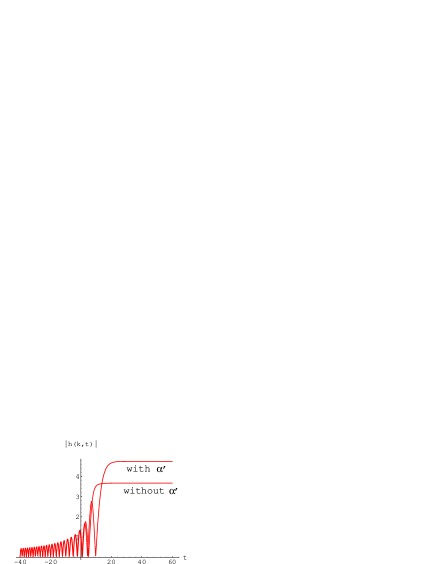
Figure 6: Amplification of tensor fluctuations, with and without the higher-curvature corrections included in the canonical perturbation equation.

The qualitative behaviour is similar, both with and without $\alpha^{\prime}$ corrections in the perturbed equations: the fluctuations are oscillating inside the horizon and frozen outside the horizon, as usual. However, the final amplitude is enhanced when $\alpha^{\prime}$ corrections are included, and this suggests that the energy spectrum of the gravitational radiation, computed with the low-energy perturbation equation, may represent a sort of lower bound on the total amount of produced gravitons.

5.4 Computation of the spectrum

The final, amplified perturbation spectrum is to be obtained from the solutions of the canonical equation (5.37). In order to solve such an equation we need explicitly the effective potential $V[z(\eta)]$ which, in general, vanishes asymptotically at large postive and negative values of the conformal time. Consider, for instance, the tensor perturbation equation in the E-frame, so that the pump field is simply the scale factor. The typical cosmological bckground in which we are interested in should describe a transition fom an initial accelerated, inflationary evolution,

$$\eta\rightarrow-\infty,~{}~{}~{}~{}~{}~{}~{}~{}~{}~{}a\sim|\eta|^{\alpha},~{}~{}~{}~{}~{}~{}~{}~{}~{}~{}V\sim\eta^{-2},$$ (5.41)

to a final standard, radiation-dominated phase,

$$\eta\rightarrow+\infty,~{}~{}~{}~{}~{}~{}~{}~{}~{}~{}a\sim\eta,~{}~{}~{}~{}~{}~{}~{}~{}~{}~{}V=0.$$ (5.42)

In this context, the evolution of fluctuations, initially normalized as in eq. (5.39), can be described as a scattering of the canonical variable by an effective potential, according to the Schrodinger-like perturbation equation (5.37) (see Fig. 7).

However, the differential variable in eq. (5.37) is (conformal) time, not space. As a consequence, the eigenfrequencies represent (comoving) energies, not momenta. Thus, even normalizing the initial state to a positive frequency mode, as in eq. (5.39), the final state is in general a mixture of positive and negative frequency modes, i.e. of positive and negative energy states,

$$\eta\rightarrow+\infty,~{}~{}~{}~{}~{}~{}~{}~{}~{}\psi_{\rm out}\sim c_{+}e^{-ik\eta}+c_{-}e^{+ik\eta}.$$ (5.43)

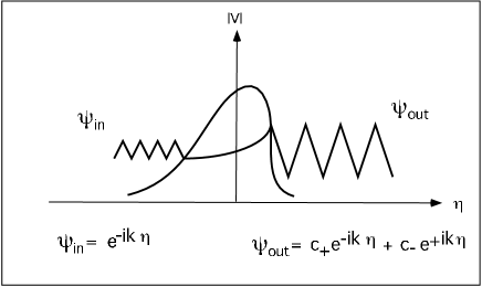
Figure 7: Scattering and amplification of the canonical variable.

In a quantum field theory context, such a mixing represents a process of pair production from the vacuum. The coefficients $c_{\pm}$ are the so-called Bogoliubov coefficients, parametrizing a unitary transformation between $|{\rm in}\rangle$ and $|{\rm out}\rangle$ states. In matrix form, they connect the set of $|{\rm in}\rangle$ annihilation and creation operators, $\{\psi_{\rm in},b_{k},b_{k}^{\dagger}\}$ to the out ones $\{\psi_{\rm out},a_{k},a_{k}^{\dagger}\}$, as follows:

$$a_{k}=c_{+}b_{k}+c_{-}^{\ast}b_{-k}^{\dagger},~{}~{}~{}~{}~{}~{}a_{-k}^{\dagger}=c_{-}b_{k}+c_{+}^{\ast}b_{-k}^{\dagger}.$$ (5.44)

Thus, even starting from the vacuum,

$$\overline{n}_{\rm in}=\langle 0|b^{\dagger}b|0\rangle=0,$$ (5.45)

we end up with a final number of produced pairs which is nonzero, in general, and is controlled by the Bogoliubov coefficient $c_{-}$ as

$$\overline{n}_{\rm out}=\langle 0|a^{\dagger}a|0\rangle=|c_{-}|^{2}\not=0.$$ (5.46)

In a second quantization approach, the amplification of perturbations can thus be seen as a process of pair production from the vacuum (or from any otherwise specified initial state), under the action of a time-dependent external field (the gravi-dilaton background, in the string cosmology case). Equivalently, the process can be described as a “squeezing” of the initial state [58] (this description is useful to evaluate the associated entropy production [59]), or, in a semiclassical language, as a “parametric amplification” [60] of the wave function $\psi_{k}$, which is scattered by an effective potential barrier through an “anti-tunnelling” process [61]. Quite independently of the adopted language, the differential energy density of the produced radiation, for each mode $k$, depends on the number of produced pairs, and can be written as

$$d\rho_{k}=2k\overline{n}_{k}{d^{3}k\over(2\pi)^{3}},~{}~{}~{}~{}~{}~{}~{}~{}~{}~{}\overline{n}_{k}=|c_{-}(k)|^{2}.$$ (5.47)

The computation of the so-called energy spectrum, defined as the spectral energy density per logarithmic interval of frequency,

$${d\rho_{k}\over d\ln k}\equiv k{d\rho_{k}\over dk}={k^{4}\over\pi^{2}}|c_{-}(k)|^{2},$$ (5.48)

thus requires the computation of $c_{-}(k)$, and then the knowledge of the asymptotic solution of the canonical pertubation equation at large positive times.

To give an explicit example we shall consider here a very simple model consisting of two cosmological phases, an initial accelerated evolution up to the time $\eta_{1}$, and a subsequent radiation-dominated evolution for $\eta>\eta_{1}$:

$$a\sim(-\eta)^{\alpha},~{}~{}~{}~{}~{}~{}~{}~{}~{}~{}~{}~{}~{}~{}~{}~{}\eta<\eta_{1},$$

$$a\sim\eta,~{}~{}~{}~{}~{}~{}~{}~{}~{}~{}~{}~{}~{}~{}~{}~{}~{}~{}~{}~{}~{}~{}\eta>\eta_{1}.$$ (5.49)

The effective potential for tensor perturbations in the E-frame, $|a^{\prime\prime}/a|$, starts from zero at $-\infty$, grows like $\eta^{-2}$, reaches a maximum $\sim\eta_{1}^{-2}$, and vanishes in the radiation phase. We must solve the canonical perturbation equation for $\eta<\eta_{1}$ and $\eta>\eta_{1}$. In the first phase the equation reduces to a Bessel equation:

$$\psi_{k}^{\prime\prime}+\left[k^{2}-{\alpha(\alpha-1)\over\eta^{2}}\right]\psi_{k}=0,$$ (5.50)

with general solution [62]

$$\psi_{k}=|\eta|^{1/2}\left[AH_{\nu}^{(2)}(|k\eta|)+BH_{\nu}^{(1)}(|k\eta|)\right],~{}~{}~{}~{}~{}~{}\nu=|\alpha-1/2|,$$ (5.51)

where $H_{\nu}^{(1,2)}$ are the first and second kind Hankel functions, of argument $k\eta$ and index $\nu=|\alpha-1/2|$ determined by the kinematics of the background. By using the large argument limit of the Hankel functions for $\eta\rightarrow-\infty$,

$$H_{\nu}^{(2)}(k\eta)\sim{1\over\sqrt{k\eta}}e^{-ik\eta},~{}~{}~{}~{}~{}~{}~{}~{}~{}~{}~{}~{}H_{\nu}^{(1)}(k\eta)\sim{1\over\sqrt{k\eta}}e^{+ik\eta},$$ (5.52)

we choose initially a positive frequency mode, normalizing the solution to a vacuum fluctuation spectrum,

$$A=1/2,~{}~{}~{}~{}~{}~{}~{}~{}~{}~{}~{}B=0.$$ (5.53)

In the second phase $V=0$, and we have the free oscillating solution :

$$\psi_{k}={1\over\sqrt{k}}\left(c_{+}e^{-ik\eta}+c_{-}e^{+ik\eta}\right).$$ (5.54)

The matching of $\psi$ and $\psi^{\prime}$ at $\eta=\eta_{1}$ gives now the coefficients $c_{\pm}$ (more precisely, the matching would require the continuity of the perturbed metric projected on a spacelike hypersurface containing $\eta_{1}$, and the continuity of the extrinsic curvature of that hypersurface [63]; but in many cases these conditions are equivalent to the continuity of the canonical variable $\psi$, and of its first time derivative).

For an approximate determination of the spectrum, which is often sufficient for pratical purposes, it is convenient to distinguish two regimes, in which the comoving frequency $k$ is much higher or much lower than the frequency associated to the top of the effective potential barrier, $|V(\eta_{1})|^{1/2}\simeq\eta_{1}^{-1}$. In the first case, $k\gg{1/|\eta_{1}|}\equiv k_{1}$, we can approximate the Hankel functions with their large argument limit, and we find that there is no particle production,

$$|c_{+}|\simeq 1,~{}~{}~{}~{}~{}~{}~{}~{}~{}~{}|c_{-}|\simeq 0.$$ (5.55)

In practice, $c_{-}$ is not exactly zero, but is exponentially suppressed as a function of the frequency, just like the quantum reflection probability for a wave with a frequency well above the top of a potential step. We will neglect such an effect here, as we are mainly interested in a qualitative estimate of the perturbation spectrum.

In the second case, $k\ll{1/|\eta_{1}|}\equiv k_{1}$, we can use the small argument limit of the Hankel functions,

$$H_{\nu}^{(2)}\sim a(k\eta_{1})^{\nu}-ib(k\eta_{1})^{-\nu},~{}~{}~{}~{}~{}~{}~{}~{}~{}~{}H_{\nu}^{(1)}\sim a(k\eta_{1})^{\nu}+ib(k\eta_{1})^{-\nu},$$ (5.56)

and we find

$$|c_{+}|\simeq|c_{-}|\simeq|k\eta_{1}|^{-\nu-1/2},$$ (5.57)

corresponding to a power-law spectrum:

$${d\rho_{k}\over d\ln k}={k^{4}\over\pi^{2}}|c_{-}(k)|^{2}\simeq{k_{1}^{4}\over\pi^{2}}\left(k\over k_{1}\right)^{3-2\nu},~{}~{}~{}~{}~{}~{}~{}~{}~{}~{}~{}~{}k<k_{1},$$ (5.58)

with a cut-off frequency $k_{1}=\eta_{1}^{-1}$ controlled by the height of the effective potential.

For a comparison with present observations, it is finally convenient to express the spectrum in terms of the proper frequency, $\omega(t)=k/a(t)$, and in units of critical energy density, $\rho_{c}(t)=3M_{p}^{2}H^{2}(t)/8\pi$. We then obtain the dimensionless spectral distribution,

$$\Omega(\omega,t)={\omega\over\rho_{c}(t)}{d\rho(\omega)\over d\omega} \simeq {8\over 3\pi}{\omega_{1}^{4}\over M_{p}^{2}H^{2}}\left(\omega\over\omega_{1}\right)^{3-2\nu}$$ (5.59)

$$\simeq g_{1}^{2}\Omega_{\gamma}(t)\left(\omega\over\omega_{1}\right)^{3-2\nu},~{}~{}~{}~{}~{}~{}~{}~{}~{}\omega<\omega_{1},$$

where

$$\omega_{1}={k_{1}\over a}={1\over a\eta_{1}}\simeq{H_{1}a_{1}\over a}$$ (5.60)

is the maximal amplified proper frequency, $g_{1}=H_{1}/M_{p}$, and

$$\Omega_{\gamma}(t)={\rho_{\gamma}\over\rho_{c}}=\left(H_{1}\over H\right)^{2}\left(a_{1}\over a\right)^{4}$$ (5.61)

is the energy density (in critical units) of the radiation that becomes dominant at $t=t_{1}$, rescaled down at a generic time $t$ (today, $\Omega_{\gamma}(t_{0})\sim 10^{-4}$).

It is important to stress that the amplitude of the spectrum is controlled by $g_{1}=H_{1}/M_{p}$, i.e. by the curvature scale in Planck units at the time of the transition $t_{1}$ (a fundamental parameter of the given inflationary model). The slope of the spectrum, $3-2\nu$, is instead controlled by the kinematics of the background. In fact, it depends on the Bessel index $\nu$ which, in its turn, depends on $\alpha$, the power of the scale factor (eq. (5.51). The behaviour in frequency of the graviton spectrum, in particular, tends to follow the behaviour of the curvature scale during the epoch of accelerated evolution, see Table III.

	scale factor	Bessel index	spectrum
de Sitter, constant curvature	$\alpha=-1$	$3-2\nu=0$	flat
power-inflation, decreasing curvature	$\alpha<-1$	$3-2\nu<0$	decreasing
pre-big bang inflation, growing curvature	$\alpha>-1$	$3-2\nu>0$	increasing

Table 3: Slope of the graviton spectrum.

The standard inflationary scenario is thus characterized by a flat or decreasing graviton spectrum; in string cosmology, instead, we must expect a growing spectrum. This has important phenomenological implications, that will be discussed in the following section.

6 The relic graviton background

As discussed in the previous Section, one of the most firm predictions of all inflationary models is the amplification of the traceless, transverse part of the quantum fluctuations of the metric tensor, and the formation of a primordial, stochastic background of relic gravitational waves, distributed over a quite large range of frequencies (see [64] for a discussion of the stochastic properties of such a background, and [65] for a possible detection of the associated “squeezing” [66]).

In a string cosmology context, the expected graviton background has been already discussed in a number of detailed review papers [61, 67, 68]. Here I will summarize the main properties of the background predicted in the context of the pre-big bang scenario.

For a phenomelogical discussion of the spetrum, it is convenient to consider the plane $\{\Omega_{G},\omega\}$. In this plane there are three main phenomenological constraints:

• A first constraint comes from the large scale isotropy of the CMB radiation. The degree of anisotropy measured by COBE imposes a bound on the energy density of the graviton background at the scale of the present Hubble radius [69],

  $$\Omega_{G}(\omega_{0})~{}\raise 1.72218pt\hbox{$<$}\kern-8.00003pt\lower 2.6694pt\hbox{$\sim$}~{}10^{-10},~{}~{}~{}~{}~{}~{}~{}~{}~{}~{}~{}~{}~{}~{}~{}~{}~{}\omega_{0}\sim 10^{-18}~{}{\rm Hz}.$$ (6.1)

• A second constraint comes from the absence of distortion of the pulsar timing-data [70], and gives the bound

  $$\Omega_{G}(\omega_{p})~{}\raise 1.72218pt\hbox{$<$}\kern-8.00003pt\lower 2.6694pt\hbox{$\sim$}~{}10^{-8},~{}~{}~{}~{}~{}~{}~{}~{}~{}~{}~{}~{}~{}~{}~{}~{}~{}\omega_{p}\sim 10^{-8}~{}{\rm Hz}.$$ (6.2)

• A third constraint comes from nucleosynthesys [71], which implies that the total graviton energy density, integrated over all modes, cannot exceed the energy density of one massless degree of freedom in thermal equilibrium, evaluated at the nucleosynthesis epoch. This gives a bound for the peak value of the spectrum [35],

  $$h_{100}\int d\ln\omega\Omega_{G}(\omega,t_{0})~{}\raise 1.72218pt\hbox{$<$}\kern-8.00003pt\lower 2.6694pt\hbox{$\sim$}~{}0.5\times 10^{-5},$$

  $$h_{100}=H_{0}/(100~{}{\rm km~{}sec}^{-1}{\rm Mpc}^{-1}),$$ (6.3)

  which applies to all scales.

A further bound can be obtained by considering the production of primordial black holes [72]. The production of gravitons, in fact, could be associated to the formation of black holes, whose possible evaporation, at the present epoch, is constrained by a number of astrophysical observations. The absence of evaporation imposes an indirect upper limit on the graviton background. In a string cosmology context, however, and in the frequency range of interest for observations, this upper limit is roughly of the same order as the nucleosynthesis bound [72].

For flat or decreasing spectra it is now evident that the more constraining bound is the low-frequency one, obtained from the COBE data. In the standard inflationary scenario, characterized by flat or decreasing spectra (see Table III), the maximal allowed graviton background can thus be plotted as in Fig. 8. The flat spectrum corresponds to de Sitter inflation, the decreasing spectra to power inflation. The breakdown in the spectrum, around $\omega_{e}q\sim 10^{-16}$ Hz, is due to the transition from the radiation-dominated to the matter-dominated phase, which only affects the low-frequency part of the spectrum, namely those modes re-entering the horizon in the matter-dominated era. For such modes there is an additional potential barrier in the canonical perturbation equation, which induces an additional amplification $\sim(\omega_{e}q/\omega)^{2}>1$, with respect to the flat de Sitter spectrum.

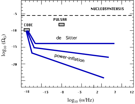
Figure 8: Graviton spectra in the standard inflationary scenario.

However, this break of the spectrum is not important for our purposes. What is important is the fact that the observed anisotropy constrains the maximal amplitude of the spectrum. But the amplitude depends on the inflation scale, as stressed in the previous Section. From the COBE bound (6.1), imposed on the modified de Sitter spectrum at the Hubble scale,

$$\Omega_{G}(\omega_{0},t_{0})=g_{1}^{2}\Omega_{\gamma}(t)(\omega_{e}q/\omega)^{2}~{}\raise 1.72218pt\hbox{$<$}\kern-8.00003pt\lower 2.6694pt\hbox{$\sim$}~{}10^{-10},$$ (6.4)

we thus obtain a direct constraint on the inflation scale:

$$H_{1}/M_{p}~{}\raise 1.72218pt\hbox{$<$}\kern-8.00003pt\lower 2.6694pt\hbox{$\sim$}~{}10^{-5}$$ (6.5)

(for power-inflation the bound is even stronger [33]).

This bound applies to all models characterized by a flat or decreasing spectrum. The bound can be evaded, however, if the spectrum is growing, like in the string cosmology context. To illustrate this point, let me consider the simplest class of the so-called “minimal” pre-big bang models, characterized by three main kinematic phases [34, 46]: an initial low-energy, dilaton-driven phase, an intermediate high-energy “string” phase, in which $\alpha^{\prime}$ and loop corrections become important, and a final standard, radiation-dominated phase (see Fig. 9). The time scale $\eta_{s}$ marks the transition to the high curvature phase, and the time scale $\eta_{1}$, characterized by a final curvature of order one in string units, marks the transition to the radiation-dominated cosmology.

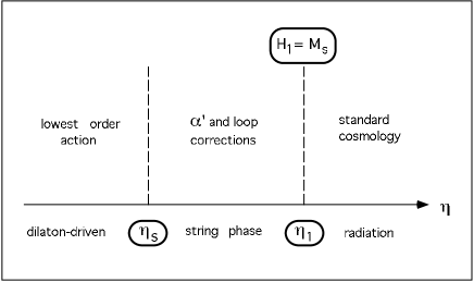
Figure 9: A minimal model of pre-big bang background.

By computing graviton production in this background [34] we find that the spectrum is characterized by two branches: a high frequency branch, for modes crossing the horizon (or “hitting” the barrier) in the string phase, $\omega>\omega_{s}=(a\eta_{s})^{-1}$; and a low frequency branch, for modes crossing the horizon in the initial dilaton phase, $\omega<\omega_{s}$. The slope is cubic at low frequency, and flatter at high frequency, and the spectrum can be parametrized as follows:

$$\Omega_{G}(\omega,t_{o}) \simeq g_{1}^{2}\Omega_{\gamma}(t_{0})\left(\omega\over\omega_{1}\right)^{3-2\nu},~{}~{}~{}~{}~{}~{}~{}~{}~{}~{}~{}~{}~{}~{}~{}~{}~{}~{}~{}~{}~{}~{}~{}~{}~{}\omega_{s}<\omega<\omega_{1},$$ (6.6)

$$\simeq g_{1}^{2}\Omega_{\gamma}(t_{0})\left(\omega_{1}\over\omega_{s}\right)^{2\nu}\left(\omega\over\omega_{1}\right)^{3},~{}~{}~{}~{}~{}~{}~{}~{}~{}~{}~{}~{}~{}~{}~{}~{}~{}~{}~{}\omega<\omega_{s}$$

(modulo logarithmic corrections). There are two main parameters: the transition frequency $\omega_{s}$, and the Bessel index $\nu$, for the high frequency part of the spectrum. These parameters represent our present ignorance about the duration and the kinematic details of the high curvature phase.

In spite of this uncertainty, however, there is a rather precise prediction for the height and the position of the peak of the spectrum, which turns out to be fixed in terms of the fundamental ratio $M_{s}/M_{p}$ as:

$$\Omega_{G}(\omega_{1})\sim 10^{-4}(M_{s}/M_{p})^{2},~{}~{}~{}~{}~{}~{}~{}~{}~{}~{}~{}~{}~{}~{}~{}\omega_{1}\sim 10^{11}(M_{s}/M_{p})^{1/2}~{}{\rm Hz}.$$ (6.7)

The behaviour of the spectrum, in this class of models, is illustrated in Fig. 10. A precise computation [35] shows that, given the maximal expected value of the string scale [15] ($M_{s}/M_{p}\simeq 0.1$), the peak value is automatically compatible with the nucleosynthesis bound, as well as with bounds from the production of primordial black holes.

In the minimal models the position of the peak is fixed. Actually, what is really fixed, in string cosmology, is the maximal height of the peak, but not necessarily the position in frequency, and it is not impossible, in more complicated non-minimal models, to shift the peak at lower frequencies.

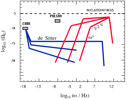
Figure 10: Graviton spectra in minimal pre-big bang models.

In minimal models, in fact, the beginning of the radiation phase coincides with the end of the string phase. We may also consider models, however, in which the dilaton coupling $g_{s}^{2}=\exp(\phi)$ is still small at the end of the high curvature phase, and the radiation era begins much later, when $g_{s}^{2}\sim 1$, after an intermediate dilaton-dominated regime. The main difference between the two cases is that in the second case the effective potential which amplifies tensor perturbations is non-monotonic [61], so that there are high frequency modes re-entering the horizon before the radiation era. As a consequence, the perturbation spectrum is also non-monotonic, and the peak does not coincide any longer, in general, with the end point of the spectrum (see also [73]), as illustrated in Fig. 11.

For minimal models the peak is around $100$ GHz, for non minimal models it could be at lower frequencies. These are good news from an experimental point of view, of course, but non-minimal models seem to be less natural, at least from a theoretical point of view. The boxes around the peak, appearing in Fig. 11, represent the uncertainty in the position of the peak due to our present ignorance about the precise value of the ratio $M_{s}/M_{p}$ (for the illustrative purpose of Fig. 11, the ratio is assumed to vary in the range $0.1-0.01$). The wavy line, in the high frequency branch of the spectrum, represents the fact that the spectrum associated to the string phase could be monotonic on the average, but locally oscillating [74]. Finally, the lower strip, labelled by $\delta s=99\%$, represents the fact that even the height of the peak could be lower than expected, if the produced gravitons have been diluted by some additional reheating phase, occurring well below the string scale, during the standard evolution.

This last effect can be parameterized in terms of $\delta s$, which is the fraction of present entropy density in radiation, due to such additional, low-scale reheating. The position of the peak then depends on $\delta s$ as [35]:

$$\omega_{1}(t_{0})\simeq T_{0}\left(M_{s}\over M_{P}\right)^{1/2}\left(1-\delta s\right)^{1/3},$$

$$\Omega_{G}(\omega_{1},t_{0})\simeq 7\times 10^{-5}h_{100}^{-2}\left(M_{s}\over M_{P}\right)^{2}\left(1-\delta s\right)^{4/3},$$ (6.8)

where $T_{0}=2.7{}^{0}K\simeq 3.6\times 10^{11}{\rm Hz}$. Such a dependence is not dramatic, however, because even for $\delta s=99\%$ the peak keeps well above the standard inflationary prediction, represented by the line labelled “de Sitter” in Fig. 11.

Given the various theoretical uncertainties, the best we can do, at present, is to define the maximal allowed region for the expected graviton background, i.e. the region spanned by the spectrum when all its parameters are varied. Such a region is illustrated in Fig. 12, for the phenomenologically interesting high frequency range. The figure emphasizes the possible, large enhancement (of about eight orders of magnitude) of the intensity of the background in string cosmology, with respect to the standard inflationary scenario.

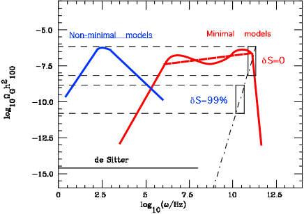
Figure 11: Peak and end point of the spectrum in minimal and non-minimal models.

It may be useful to stress again the reason of such enhancement. In the standard inflationary scenario the graviton spectrum is decreasing, the normalization is imposed at low frequency, and the peak value is contolled by the anisotropy of the CMB radiation, $\delta T/T~{}\raise 1.72218pt\hbox{$<$}\kern-8.00003pt\lower 2.6694pt\hbox{$\sim$}~{}10^{-5}$. Thus, at low frequency,

$$\Omega_{G}(t_{0})~{}\raise 1.72218pt\hbox{$<$}\kern-8.00003pt\lower 2.6694pt\hbox{$\sim$}~{}\Omega_{\gamma}(t_{0})\left(\Delta T\over T\right)^{2}_{COBE}\sim 10^{-14}.$$ (6.9)

In string cosmology the spectrum is growing, the normalization is imposed at high frequency, and the peak value is controlled by the fundamental ratio $M_{s}/M_{p}~{}\raise 1.72218pt\hbox{$<$}\kern-8.00003pt\lower 2.6694pt\hbox{$\sim$}~{}0.1$. Thus

$$\Omega_{G}(t_{0})~{}\raise 1.72218pt\hbox{$<$}\kern-8.00003pt\lower 2.6694pt\hbox{$\sim$}~{}\Omega_{\gamma}(t_{0})\left(M_{s}\over M_{p}\right)^{2}~{}\raise 1.72218pt\hbox{$<$}\kern-8.00003pt\lower 2.6694pt\hbox{$\sim$}~{}10^{-6}.$$ (6.10)

The graviton background obtained from the amplification of the vacuum fluctuations, in string cosmology and in standard inflation, is compared in Fig. 12 with other, more unconventional graviton spectra. In particular: the graviton spectrum obtained from cosmic strings and topological defects [75], from bubble collision at the end of a first order phase transition [76], and from a phase of parametric resonance of the inflaton oscillations [77]. Also shown in Fig. 12 is the spectrum from models of quintessential inflation [78], and a thermal black body spectrum for a temperature of about one kelvin. All these cosmological backgrounds are higher than the background expected from the vacuum fluctuations in standard inflation, but not in a string cosmology context.

It may be interesting, at this point, to recall the expected sensitivities of the present, and near future, gravitational antennas, referred to the plots of Fig. 12.

At present, the best direct, experimental upper bound on the energy of a stochastic graviton background comes from the cross-correlation of the data of the two resonant bars NAUTILUS and EXPLORER [79]:

$$\Omega_{G}h_{100}~{}\raise 1.72218pt\hbox{$<$}\kern-8.00003pt\lower 2.6694pt\hbox{$\sim$}~{}60,~{}~{}~{}~{}~{}~{}~{}~{}~{}~{}~{}~{}~{}~{}~{}~{}~{}~{}~{}\nu\simeq 907~{}{\rm Hz}$$ (6.11)

(similar sensitivities are also reached by AURIGA [80]). Unfortunately, the bound is too high to be significant for the plots of Fig. 12. However, a much better sensitivity, $\Omega_{G}\sim 10^{-4}$ around $\nu\sim 10^{3}$ Hz, is expected from the present resonant bar detectors, if the integration time of the data is extended to about one year. A similar, or slightly better sensitivity, $\Omega_{G}\sim 10^{-5}$ around $\nu\sim 10^{2}$ Hz, is expected from the first operating version of the interferometric detectors, such as LIGO and VIRGO. At high frequency, from the kHz to the MHz range, a promising possibility seems to be the use of resonant electromagnetic cavities as gravity wave detectors [81]. Work is in progress [82] to attempt to improve their sensitivity.

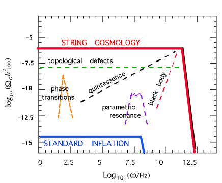
Figure 12: Allowed region for the spectrum of vacuum fluctuations in string cosmology and in standard inflation, compared with other relic spectra of primordial origin.

The present, and near future, available sensitivities of resonant bars and interferometers, therefore, are still outside the allowed region of Fig. 12, determined by the border line

$$\Omega_{G}h_{100}\simeq 10^{-6}.$$ (6.12)

Such sensitivities are not so far from the border, after all, but to get really inside we have to wait for the cross-correlation of two spherical resonant-mass detectors [83], expected to reach $\Omega_{G}\sim 10^{-7}$ in the kHz range, or for the advanced interferometers, expected to reach $\Omega_{G}\sim 10^{-10}$ in the range of $10^{2}$ Hz. At lower frequencies, around $10^{-2}-10^{-3}$ Hz, the space interferometer LISA [38] seem to be able to reach very high sensitivities, up to $\Omega_{G}\sim 10^{-11}$. Work is in progress, however, for a more precise computation of their sensitivity to a cosmic stochastic background [84].

Detectors able to reach, and to cross the limiting sensitivity (6.12), could explore for the first time the parameter space of string cosmology and of Planck scale physics. The detection of a signal from a pre-big bang background, extrapolated to the GHz range, could give a first experimental indication on the value of the fundamental ratio $M_{s}/M_{p}$. Even the absence of a signal, inside the allowed region, would be significant, as we could exclude some portion of parameter space of the string cosmlogy models, obtaining in such a way direct experimental information about processes occuring at (or very near to) the string scale.

7 Conclusion

The conclusion of these lectures is very short and simple.

There is a rich structure of stochastic, gravitational wave backgrounds, of cosmological origin, in the frequency range of present (or planned for the future) gravity wave detectors.

Among such backgrounds, the stronger one seems to be the background possibly predicted in the context of the pre-big bang scenario, in a string cosmology context, originating at (or very near to) the fundamental string scale. Also, the maximal predicted intensity of the background seems to be accessible to the sensitivity of the future advanced detectors.

If this is the case, the future gravity wave detectors will be able to test string theory models, or perhaps models referring to some more fundamental unified theory, such as D-brane theory, M-theory, and so on. In any case, such detectors will give direct experimental information on Planck scale physics.

Appendix A The string effective action

The motion of a point particle in an external gravitational field, $g_{\mu\nu}$, is governed by the action

$$S=-{m\over 2}\int d\tau\dot{x}^{\mu}\dot{x}^{\nu}g_{\mu\nu}(x),$$ (1.1)

where $x^{\mu}(\tau)$ are the spacetime coordinates of the particle, and $\tau$ is an affine parameter along the particle world-line.

The time evolution of a one-dimensional object like a string describes a world-surface, or “world-sheet”, instead of a world-line, and the action governing its motion is given by the surface integral

$$S=-{M_{s}^{2}\over 2}\int d\tau d\sigma\sqrt{-\gamma}\gamma^{ij}\partial_{i}x^{\mu}\partial_{j}x^{\nu}g_{\mu\nu}(x),$$ (1.2)

where $\partial_{i}\equiv\partial/\partial\xi^{i}$, and $\xi^{i}=(\tau,\sigma)$ are respectively the timelike and spacelike coordinate on the string world-sheet ($i,j=1,2$). The coordinates $x^{\mu}(\tau,\sigma)$ are the fields governing the embedding of the string world-sheet in the external (also called “target”) space. The parameter $M_{s}^{2}$ defines (in units $h/2\pi=1=c$) the so-called string tension (the mass per unit length), and its inverse defines the fundamental length scale of the theory (often called, for hystorical reasons, the $\alpha^{\prime}$ parameter):

$$M_{s}^{2}\equiv{1\over\lambda_{s}^{2}}\equiv{1\over 2\pi\alpha^{\prime}}.$$ (1.3)

In a curved metric background $g_{\mu\nu}$ depends on $x^{\mu}$, and the nonlinear action (1.2) represents what is called a “sigma model” defined on the string world sheet.

For the point particle action (1.1) the variation with respect to $x^{\mu}$ leads to the well known geodesic equations of motion,

$$\ddot{x}^{\mu}+\Gamma_{\alpha\beta}\,^{\mu}\dot{x}^{\alpha}\dot{x}^{\beta}=0.$$ (1.4)

The string equations of motion are similarly obtained by varying with respect to $x^{\mu}$ the action (1.2): we get then the Eulero-Lagrange equations

$$\partial_{i}{\partial L\over\partial(\partial_{i}x^{\mu})}={\partial L\over\partial x^{\mu}},~{}~{}~{}~{}~{}~{}~{}~{}~{}~{}L=\sqrt{-\gamma}\gamma^{ij}\partial_{i}x^{\mu}\partial_{j}x^{\nu}g_{\mu\nu},$$ (1.5)

which can be written explicitly as

$$\hbox to1.0pt{\hfill}\mathchoice{\vbox{\hrule height=0.4pt\hbox{\vrule width=0.4pt,height=8.0pt\kern 8.0pt\vrule width=0.4pt} \hrule height=0.4pt}}{\vbox{\hrule height=0.4pt\hbox{\vrule width=0.4pt,height=8.0pt\kern 8.0pt\vrule width=0.4pt} \hrule height=0.4pt}}{\vbox{\hrule height=0.4pt\hbox{\vrule width=0.4pt,height=8.0pt\kern 8.0pt\vrule width=0.4pt} \hrule height=0.4pt}}{\vbox{\hrule height=0.4pt\hbox{\vrule width=0.4pt,height=8.0pt\kern 8.0pt\vrule width=0.4pt} \hrule height=0.4pt}}\hbox to1.0pt{\hfill}x^{\mu}+\gamma^{ij}\partial_{i}x^{\alpha}\partial_{j}x^{\beta}\Gamma_{\alpha\beta}\,^{\mu}=0,~{}~{}~{}~{}~{}~{}~{}~{}~{}~{}~{}\hbox to1.0pt{\hfill}\mathchoice{\vbox{\hrule height=0.4pt\hbox{\vrule width=0.4pt,height=8.0pt\kern 8.0pt\vrule width=0.4pt} \hrule height=0.4pt}}{\vbox{\hrule height=0.4pt\hbox{\vrule width=0.4pt,height=8.0pt\kern 8.0pt\vrule width=0.4pt} \hrule height=0.4pt}}{\vbox{\hrule height=0.4pt\hbox{\vrule width=0.4pt,height=8.0pt\kern 8.0pt\vrule width=0.4pt} \hrule height=0.4pt}}{\vbox{\hrule height=0.4pt\hbox{\vrule width=0.4pt,height=8.0pt\kern 8.0pt\vrule width=0.4pt} \hrule height=0.4pt}}\hbox to1.0pt{\hfill}\equiv{1\over\sqrt{-\gamma}}\partial_{i}\sqrt{-\gamma}\gamma^{ij}\partial_{j},$$ (1.6)

These equations describe the geodesic evolution of a test string in a given external metric. The variation with respect to $\gamma_{ik}$ imposes the so-called “costraints”, i.e. the vanishing of the world sheet stress tensor $T_{ik}$,

$$T_{ij}={2\over\sqrt{-\gamma}}{\delta S\over\delta\gamma^{ij}}=\partial_{i}x^{\mu}\partial_{j}x^{\nu}g_{\mu\nu}-{1\over 2}\gamma_{ij}\partial_{k}x^{\mu}\partial^{k}x_{\mu}=0.$$ (1.7)

It is important to note, at this point, that for a classical string it is always possible to impose the so-called “conformal gauge” in which the world sheet metric is flat, $\gamma_{ij}=\eta_{ij}$. In fact, in an appropriate basis, the two-dimensional metric tensor can always be set in a diagonal form, $\gamma_{ij}={\rm diag}(a,b)$, and then, by using reparametrization invariance on the world sheet, $b^{2}d\sigma^{2}=a^{2}d\sigma^{{}^{\prime}2}$, the metric can be set in a conformally flat form, $\gamma_{ij}=a^{2}\eta_{ij}$. Since the action (1.2) in invariant under the conformal (or Weyl) transformation $\gamma_{ij}\rightarrow\Omega^{2}(\xi_{k})\gamma_{ij}$,

$$\sqrt{-\gamma}\gamma^{ij}\rightarrow\sqrt{\Omega^{4}}~{}\Omega^{-2}\sqrt{-\gamma}\gamma^{ij},$$ (1.8)

we can always eliminate the conformal factor $a^{2}$ in front of the Minkowski metric, by choosing $\Omega=a^{-1}$. In the conformal gauge the equations of motion (1.6) reduce to

$$\ddot{x}^{\mu}-x^{\prime\prime\mu}+\Gamma_{\alpha\beta}\,^{\mu}\left(\dot{x}^{\alpha}+x^{\prime\alpha}\right)\left(\dot{x}^{\beta}-x^{\prime\beta}\right)=0,$$ (1.9)

where $\dot{x}=dx/d\tau$, $x^{\prime}=dx/d\sigma$, and the constraints (1.7) become

$$g_{\mu\nu}\left(\dot{x}^{\mu}\dot{x}^{\nu}+x^{\prime\mu}x^{\prime\nu}\right)=0,~{}~{}~{}~{}~{}~{}~{}~{}~{}g_{\mu\nu}\dot{x}^{\mu}x^{\prime\nu}=0.$$ (1.10)

We now come to the crucial observation which leads to the effective action governing the motion of the background fields. The conformal transformation (1.8) is an invariance of the classical theory. Let us require that there are no “anomalies”, i.e. no quantum violations of this classical symmetry. By imposing such a constraint, we will obtain a set of differential equations to be satisfied by the background fields coupled to the string. Thus, unlike a point particle which does not imposes any constraint on the external geometry in which it is moving, the consistent quantization of a string gives constraints for the external fields. The background geometry cannot be chosen arbitrarily, but must satisfy the set of equations(also called $\beta$-function equations) which guarantee the absence of conformal anomalies. The string effective action used in this paper is the action which reproduces such a set of equations for the background fields, and in particular for the metric.

The derivation of the background equations of motion and of the effective action, from the sigma-model action (1.2), can be performed order by order by using a perturbative expansion in powers of $\alpha^{\prime}$ (indeed, in the limit $\alpha^{\prime}\rightarrow 0$ the action becomes very large in natural units, so that the quantum corrections are expected to become smaller and smaller). Such a procedure, however, is in general long and complicated, even to lowest order, and a detailed derivation of the background equations is outside the purpose of these lectures. Let me sketch here the procedure for the simplest case in which the only external field coupled to the string is the metric tensor $g_{\mu\nu}$.

In the conformal gauge, the action (1.2) becomes:

$$S=-{1\over 4\pi\alpha^{\prime}}\int d^{2}\xi~{}\partial_{i}x^{\mu}\partial^{i}x^{\nu}g_{\mu\nu}.$$ (1.11)

Let us formally assume a deformation of the number of world sheet dimensions, from $2$ to $2+\epsilon$, and perform the conformal transformation: $\eta_{ij}\rightarrow\eta_{ij}\exp(\rho)$. Expanding we get, for small $\epsilon$,

$$-{1\over 4\pi\alpha^{\prime}}\int d^{2+\epsilon}\xi~{}e^{\rho\epsilon/2}\partial_{i}x^{\mu}\partial^{i}x^{\nu}g_{\mu\nu}=$$

$$-{1\over 4\pi\alpha^{\prime}}\int d^{2+\epsilon}\xi~{}\partial_{i}x^{\mu}\partial^{i}x^{\nu}g_{\mu\nu}\left(1+{\epsilon\over 2}\rho+...\right).$$ (1.12)

For $\epsilon\rightarrow 0$ the $\rho$ dependence disappears, and the classical action is conformally invariant. In order to preserve this invariance also for the quantum theory, at the one loop level, let us treat the sigma model as a quantum field theory for $x^{\mu}(\sigma,\tau)$, and let us consider the quantum fluctuations $\hat{x}^{\mu}$ around a given expectation value $x_{0}^{\mu}$. For the general reparametrization invariance of the theory we can always choose for $x_{0}$ a locally inertial frame, such that $g_{\mu\nu}(x_{0})=\eta_{\mu\nu}$. By expanding the metric around $x_{0}$, the leading corrections are of second order in the fluctuations, because in a locally inertial frame the first derivatives of the metric (and then the Cristoffel connection) can always be set to zero (but not the curvature). With an appropriate choice of coordinates, called Riemann normal coordinates, the metric can thus be expanded as:

$$g_{\mu\nu}(x)=\eta_{\mu\nu}-{1\over 3}R_{\mu\nu\alpha\beta}(x_{0})\hat{x}^{\alpha}\hat{x}^{\beta}+...$$ (1.13)

and the action for the quantum fluctuations becomes, to lowest order in the curvature,

$$\qquad S=-{1\over 4\pi\alpha^{\prime}}\int d^{2+\epsilon}\xi\Bigg{[}\partial_{i}\hat{x}^{\mu}\partial^{i}\hat{x}_{\mu}\left(1+{\epsilon\over 2}\rho\right)$$

$$\qquad-{1\over 3}\partial_{i}\hat{x}^{\mu}\partial^{i}\hat{x}^{\nu}R_{\mu\nu\alpha\beta}(x_{0})\hat{x}^{\alpha}\hat{x}^{\beta}\left(1+{\epsilon\over 2}\rho\right)+...\Bigg{]}.$$ (1.14)

It must be noted that, at the quantum level, the dependence of $\rho$ does not disappear in general from the action in the limit $\epsilon\rightarrow 0$, since there are one-loop terms that diverge like $\epsilon^{-1}$, just to cancel the $\epsilon$ dependence and to give a contribution proportional to $\rho$ to the effective action. By evaluating, for instance, the two point function for the quantum operator $\hat{x}^{\alpha}\hat{x}^{\beta}$, in the coincidence limit $\sigma\rightarrow\sigma^{\prime}$ (the tadpole graph), one obtains [85]

$$\langle\hat{x}^{\alpha}(\sigma)\hat{x}^{\beta}(\sigma^{\prime})\rangle_{\sigma\rightarrow\sigma^{\prime}}\sim\eta^{\alpha\beta}\lim_{\sigma\rightarrow\sigma^{\prime}}\int d^{2+\epsilon}k{e^{ik\cdot(\sigma-\sigma^{\prime})}\over k^{2}}\sim\eta^{\alpha\beta}\epsilon^{-1},$$ (1.15)

which gives the one-loop contribution to the action

$$\Delta S\sim\int d^{2+\epsilon}\xi~{}\partial_{i}\hat{x}^{\mu}\partial^{i}\hat{x}^{\nu}R_{\mu\nu}~{}\rho.$$ (1.16)

This term violates, at one-loop, the conformal invariance, unless we restrict to a background geometry satisfying the condition

$$R_{\mu\nu}=0,$$ (1.17)

which are just the usual Einstein equations in vacuum.

A similar procedure can be applied if the string moves in a richer external background (not only pure gravity). Indeed, pure gravity is not enough, as a consistent quantum theory for closed bosonic strings, for instance, must contain at least three massless state (beside the unphysical tachyon, removed by supersymmetry) in the lowest energy level: the graviton, the scalar dilaton and the pseudo-scalar Kalb-Ramond axion. The sigma model describing the propagation of a string in such a background must thus contain the coupling to the metric, to the dilaton $\phi$, and to the two-form $B_{\mu\nu}=-B_{\nu\mu}$:

$$S=-{1\over 4\pi\alpha^{\prime}}\int d^{2}\xi~{}\partial_{i}x^{\mu}\partial_{j}x^{\nu}\left(\sqrt{-\gamma}\gamma^{ij}g_{\mu\nu}+\epsilon^{ij}B_{\mu\nu}\right)$$

$$-{1\over 4\pi}\int d^{2}\xi\sqrt{-\gamma}{\phi\over 2}R^{(2)}(\gamma),$$ (1.18)

where $\epsilon^{ij}$ is the two-dimensional Levi-Civita densor density, $\epsilon_{12}=-\epsilon_{21}=1$, and $R^{(2)}(\gamma)$ is the two-dimensional scalar curvature for the world sheet metric $\gamma$. The condition of conformal invariance, at the one-loop level, leads to the equations

$$R_{\mu\nu}+\nabla_{\mu}\nabla_{\nu}-{1\over 4}H_{\mu\alpha\beta}H_{\nu}\,^{\alpha\beta}=0,~{}~{}~{}~{}H_{\mu\nu\alpha}=\partial_{\mu}B_{\nu\alpha}+\partial_{\nu}B_{\alpha\mu}+\partial_{\alpha}B_{\mu\nu},$$

$$R+2\nabla^{2}\phi-(\nabla\phi)^{2}-{1\over 12}H_{\mu\nu\alpha}^{2}=0,$$

$$\nabla_{\mu}\left(e^{-\phi}H^{\mu\nu\alpha}\right)=0,$$ (1.19)

which can be obtained by extremizing the effective action

$$S=-{1\over 2\lambda_{s}^{d-1}}\int d^{d+1}x\sqrt{|g|}~{}e^{-\phi}\left[R+\left(\nabla\phi\right)^{2}-{1\over 12}H_{\mu\nu\alpha}^{2}\right].$$ (1.20)

(see Appendix C).

It should be noted that the inclusion of the dilaton in the condition of conformal invariance cannot be avoided, since the dilaton coupling in the action (1.18) breaks conformal invariance already at the classical level ($\sqrt{-\gamma}R^{(2)}$ is not invariant under a Weyl rescaling of $\gamma$). However, the dilaton term is of order $\alpha^{\prime}$ with respect to the other terms of the action (for dimensional reasons), so that it is correct to sum up the classical dilaton contribution to the quantum, one-loop effects, as they are all of the same order in $\alpha^{\prime}$. Without the dilaton, however, the world sheet curvature density $\sqrt{-\gamma}R^{(2)}$ does not contribute to the string equations of motion, as it is a pure Eulero two-form in two dimensions (just like the Gauss-Bonnet term in four dimensions).

Let me note, finally, that the expansion around $x_{0}$ can be continued to higher orders,

$$g(x)=\eta+R\hat{x}\hat{x}+\partial R\hat{x}\hat{x}\hat{x}+R^{2}\hat{x}\hat{x}\hat{x}\hat{x}+...,$$ (1.21)

thus introducing higher curvature terms, and higher powers of $\alpha^{\prime}$, in the effective action:

$$S=-{1\over 2\lambda_{s}^{d-1}}\int d^{d+1}x\sqrt{|g|}~{}e^{-\phi}\left[R+\left(\nabla\phi\right)^{2}-{\alpha^{\prime}\over 4}R_{\mu\nu\alpha\beta}^{2}+...\right].$$ (1.22)

At any given order, unfortunately, there is an intrinsic ambiguity in the action due to the fact that, with an appropriate field redefinition of order $\alpha^{\prime}$,

$$g_{\mu\nu}\rightarrow g_{\mu\nu}+\alpha^{\prime}\left(R_{\mu\nu}+\partial_{\mu}\phi\partial_{\nu}\phi+...\right)$$

$$\phi\rightarrow\phi+\alpha^{\prime}\left(R+\nabla^{2}\phi+...\right),$$ (1.23)

we obtain a number of different actions, again of the same order in $\alpha^{\prime}$ (see for instance [86]). This ambiguity cannot be eliminated until we limit to an effective action truncated to a given finite order.

The higher curvature (or higher derivative) expansion of the effective action is typical of string theory: it is controlled by the fundamental, minimal length parameter $\lambda_{s}=(2\pi\alpha^{\prime})^{1/2}$, in such a way that the higher order corrections disappear in the point-particle limit $\lambda_{s}\rightarrow 0$. At any given order in $\alpha^{\prime}$, however, there is also the more conventional expansion in power of the coupling constant $g_{s}$ (i.e. the loop expansion of quantum field theory: tree-level $\sim g^{-2}$, one-loop $\sim g^{0}$, two-loop $\sim g^{2}$, …). The important observation is that, in a string theory context, the effective couplig constant is controlled by the dilaton. Consider, for instance, a process of graviton scattering, in four dimensions. Comparing the action (2.4) with the standard, gravitational Einstein action (2.1), it follows that the effective coupling constant, to lowest order, is

$$\sqrt{8\pi G}=\lambda_{p}=\lambda_{s}e^{\phi/2}$$ (1.24)

($G$ is the usual Newton constant). Each loop adds an integer power of the square of the dimensionless coupling constant, which is controlled by the dilaton as

$$g_{s}^{2}=(\lambda_{p}/\lambda_{s})^{2}=(M_{s}/M_{p})^{2}=e^{\phi}.$$ (1.25)

We may thus expect, for the loop expansion of the action, the following general scheme:

$$S= - \int e^{-\phi}\sqrt{-g}\left(R+\nabla\phi^{2}+\alpha^{\prime}R^{2}+...\right)~{}~{}~{}~{}~{}~{}~{}~{}~{}~{}~{}~{}~{}{\rm tree~{}level}$$ (1.26)

$$- \int\sqrt{-g}\left(R+\nabla\phi^{2}+\alpha^{\prime}R^{2}+...\right)~{}~{}~{}~{}~{}~{}~{}~{}~{}~{}~{}~{}~{}~{}~{}~{}~{}~{}{\rm one-loop}$$

$$- \int e^{+\phi}\sqrt{-g}\left(R+\nabla\phi^{2}+\alpha^{\prime}R^{2}+...\right)~{}~{}~{}~{}~{}~{}~{}~{}~{}~{}~{}~{}~{}{\rm two-loop}$$

$$............................$$

Unfortunately, each term in the action, at each loop order, is multiplied by a dilaton “form factor” which is different in general for different fields and for different orders. This difference can lead to an effective violation of the universality of the gravitational interactions [87] in the low-energy, macroscopic regime, and this violation can be reconciled with the present tests of the equivalence principle only if the dilaton is massive enough, to make short enough the range of the non-universal dilatonic interactions.

The tree-level relation (1.25) is valid also for a higher-dimensional effective action, provided $e^{\phi}$ represents the shifted four-dimensional dilaton which includes the volume of the extra-dimensional, compact internal space, and which controls the grand-unification gauge coupling, $\alpha_{GUT}$, as [15]

$$\alpha_{GUT}=\exp\langle\phi\rangle=(M_{s}/M_{p})^{2}\sim 0.1-0.001.$$ (1.27)

However, the relation (1.25) is no longer valid, in general, if the gauge interactions are confined in four-dimensions and only gravity propagates in the extra dimensions. In that case the relation depends on the volume of the extra dimensions, whose size may be allowed to be large in Planck units [88]. For internal dimensions of volume $V_{n}$ the relation becomes, in particular,

$$M_{p}^{2}=M_{s}^{2+n}V_{n}e^{-\Phi},$$ (1.28)

where $\Phi$ is the dilaton in $d=3+n$ dimensions. In this case, the string mass parameter could be much smaller than the value expected from eq. (1.27), provided the internal volume is correspondingly larger.

Appendix B Duality symmetry

Notations and conventions. In this paper we use the metric signature $(+---)$, and we define the Riemann and Ricci tensor as follows:

$$R_{\mu\nu\alpha}\,^{\beta}=\partial_{\mu}\Gamma_{\nu\alpha}\,^{\beta}+\Gamma_{\mu\rho}\,^{\beta}\Gamma_{\nu\alpha}\,^{\rho}-(\mu\leftrightarrow\nu),$$

$$R_{\nu\alpha}=R_{\mu\nu\alpha}\,^{\mu}.$$

Consider the gravi-dilaton effective action, in the S-frame, to lowest order in $\alpha^{\prime}$ and in the quantum loop expansion:

$$S=-{1\over 2\lambda_{s}^{d-1}}\int d^{d+1}x\sqrt{|g|}~{}e^{-\phi}\left[R+\left(\nabla\phi\right)^{2}\right].$$ (2.1)

For a homogeneous, but anisotropic, Bianchi I type metric background:

$$\phi=\phi(t),~{}~{}~{}~{}~{}~{}~{}g_{00}=N^{2}(t),~{}~{}~{}~{}~{}~{}~{}g_{ij}=-a_{i}^{2}(t)\delta_{ij},$$ (2.2)

we have ($H_{i}=\dot{a}_{i}/a_{i}$):

$$\left(\nabla\phi\right)^{2}={\dot{\phi}^{2}\over N^{2}},~{}~{}~{}~{}~{}~{}~{}~{}~{}~{}\sqrt{-g}=N\prod_{i=1}^{d}a_{i},$$

$$\Gamma_{00}\,^{0}={\dot{N}\over N}\equiv F,~{}~{}~{}~{}~{}~{}~{}~{}~{}~{}\Gamma_{0i}\,^{j}=H_{i}\delta_{i}^{j},~{}~{}~{}~{}~{}~{}~{}~{}~{}~{}\Gamma_{ij}\,^{0}={a_{i}\dot{a}_{i}\over N^{2}}\delta_{ij},$$

$$R={1\over N^{2}}\left[2F\sum_{i}H_{i}-2\sum_{i}\dot{H}_{i}-\sum_{i}H_{i}^{2}-\left(\sum_{i}H_{i}\right)^{2}\right].$$ (2.3)

By noting that

$${d\over dt}\left[2{e^{-\phi}\over N}\left(\prod_{k=1}^{d}a_{k}\right)\left(\sum_{i}H_{i}\right)\right]$$

$$={e^{-\phi}\over N}\left(\prod_{k=1}^{d}a_{k}\right)\left[2\sum_{i}\dot{H}_{i}-2F\sum_{i}H_{i}-2\dot{\phi}\sum_{i}H_{i}+2\left(\sum_{i}H_{i}\right)^{2}\right],$$ (2.4)

the action (2.1), modulo a total derivative, can be rewritten as:

$$S=-{1\over 2\lambda_{s}^{d-1}}\int d^{d}xdt\prod_{i=1}^{d}a_{i}{e^{-\phi}\over N}\left[\dot{\phi}^{2}-\sum_{i}H_{i}^{2}+\left(\sum_{i}H_{i}\right)^{2}-2\dot{\phi}\sum_{i}H_{i}\right].$$ (2.5)

We now introduce the so-called shifted dilaton $\overline{\phi}$, defined by

$$e^{-\overline{\phi}}=\int{d^{d}x\over\lambda_{s}^{d}}\prod_{i=1}^{d}a_{i}e^{-\phi},$$ (2.6)

from which

$$\phi=\overline{\phi}+\sum_{i}\ln a_{i},~{}~{}~{}~{}~{}~{}~{}~{}~{}~{}~{}~{}\dot{\phi}=\dot{\overline{\phi}}+\sum_{i}H_{i}$$ (2.7)

(by assuming spatial sections of finite volume, $(\int d^{d}x\sqrt{|g|})_{t={\rm const}}<\infty$, we have absorbed into $\phi$ the constant shift $-\ln(\lambda_{s}^{-d}\int d^{d}x)$, required to secure the scalar behaviour of $\overline{\phi}$ under coordinate reparametrizations preserving the comoving gauge). The action becomes:

$$S=-{\lambda_{s}\over 2}\int dt{e^{-\overline{\phi}}\over N}\left(\dot{\overline{\phi}}^{2}-\sum_{i}H_{i}^{2}\right).$$ (2.8)

By inverting one of the $d$ scale factors the corresponding Hubble parameter changes sign,

$$a_{i}\rightarrow\tilde{a}_{i}=a_{i}^{-1},~{}~{}~{}~{}~{}~{}~{}~{}~{}H_{i}\rightarrow\tilde{H}_{i}={\dot{\tilde{a}_{i}}\over\tilde{a}_{i}}=a_{i}{da_{i}^{-1}\over dt}=-H_{i},$$ (2.9)

so that the quadratic action (2.8) is clearly invariant under the inversion of any scale factor preserving the shifted dilaton,

$$a_{i}\rightarrow\tilde{a}_{i}=a_{i}^{-1},~{}~{}~{}~{}~{}~{}~{}~{}~{}~{}~{}~{}~{}~{}\overline{\phi}\rightarrow\overline{\phi}$$ (2.10)

(“scale factor duality”, see [11] and the first paper of Ref. [10]).

In order to derive the field equations, it is convenient to use the variables $\beta_{i}=\ln a_{i}$, so that $H_{i}=\dot{\beta}_{i}$, $\dot{H}_{i}=\ddot{\beta}_{i}$, and the action (2.8) is cyclic in $\beta_{i}$. By varying with respect to $N,\beta_{i}$ and $\overline{\phi}$, and subsequently fixing the cosmic time gauge $N=1$, we obtain, respectively,

$$\dot{\overline{\phi}}^{2}-\sum_{i}H_{i}^{2}=0,$$ (2.11)

$$\dot{H}_{i}-H_{i}\dot{\overline{\phi}}=0,$$ (2.12)

$$2\ddot{\overline{\phi}}-\dot{\overline{\phi}}^{2}-\sum_{i}H_{i}^{2}=0.$$ (2.13)

This is a system of $(d+2)$ equations for the $(d+1)$ variables $\{a_{i},\phi\}$. However, only $(d+1)$ equations are independent (see for instance [23]: eq. (2.11) represents a constraint on the set of initial data).

The above equations are invariant under a time reversal transformation

$$t\rightarrow-t,~{}~{}~{}~{}~{}~{}~{}~{}~{}~{}H\rightarrow-H,~{}~{}~{}~{}~{}~{}~{}~{}~{}~{}\dot{\overline{\phi}}\rightarrow-\dot{\overline{\phi}},$$ (2.14)

and also under the duality transformation (2.10). If we invert $k\leq d$ scale factors, $\tilde{a}_{1}=a_{1}^{-1}$, … $\tilde{a}_{k}=a_{k}^{-1}$, the shifted dilaton is preserved, $\overline{\phi}=\tilde{\overline{\phi}}$, provided

$$\overline{\phi}=\phi-\sum_{i=1}^{d}\ln a_{i}=\tilde{\phi}-\sum_{i=1}^{k}\ln\tilde{a}_{i}-\sum_{i=k+1}^{d}\ln a_{i},$$ (2.15)

from which:

$$\tilde{\phi}=\phi-2\sum_{i=1}^{k}\ln a_{i}.$$ (2.16)

Given an exact solution, represented by the set of variables

$$\{a_{1},...a_{d},~{}\phi\},$$ (2.17)

the inversion of $k\leq d$ scale factors defines then a new exact solution, represented by the set of variables

$$\{a_{1}^{-1},...a_{k}^{-1},a_{k+1},...a_{d},~{}\phi-2\ln a_{1}...-2\ln a_{k}\}.$$ (2.18)

By inverting all the scale factors we obtain the transformation

$$\{a_{i},\phi\}\rightarrow\{a_{i}^{-1},\phi-2\sum_{i=1}^{d}\ln a_{i}\}$$ (2.19)

which, in the isotropic case, corresponds in particular to the duality transformation (2.5).

As a simple example, we consider here the particular isotropic solution

$$a=t^{1/\sqrt{d}},~{}~{}~{}~{}~{}~{}~{}~{}~{}~{}~{}~{}~{}~{}~{}\overline{\phi}=-\ln t,$$ (2.20)

which satisfies identically the set of equations (2.11) - (2.13). By applying a duality and a time-reversal transformation we obtain the four different exact solutions

$$\{a_{\pm}(t)=t^{\pm 1/\sqrt{d}},~{}~{}\overline{\phi}(t)=-\ln t\},$$

$$\{a_{\pm}(-t)=(-t)^{\pm 1/\sqrt{d}},~{}~{}\overline{\phi}(-t)=-\ln(-t)\},$$ (2.21)

corresponding to the four branches illustrated in Fig. 2, and describing decelerated expansion, $a_{+}(t)$, decelerated contraction, $a_{-}(t)$, accelerated contraction, $a_{+}(-t)$, accelerated expansion, $a_{-}(-t)$. The solution describes expansion or contraction if the sign of $\dot{a}$ is positive or negative, repectively, and the solution is accelerated or decelerated if $\dot{a}$ and $\ddot{a}$ have the same or the opposite sign, respectively.

It is important to consider also the dilaton behaviour. According to eq. (2.7):

$$\phi_{\pm}(\pm t)=\overline{\phi}(\pm t)+d\ln a_{\pm}(\pm t)=\left(\pm\sqrt{d}-1\right)\ln(\pm t).$$ (2.22)

It follows that, in a phase of growing curvature ($t<0,t\rightarrow 0_{-}$), the dilaton is growing only for an expanding metric, $a_{-}(-t)$. This means that, in the isotropic case, there are only expanding pre-big bang solution, i.e. solutions evolving from the string perturbative vacuum ($H\rightarrow 0,\phi\rightarrow-\infty$), and then characterized by a growing string coupling, $\dot{g}_{s}=(\exp\phi/2)\dot{}>0$.

In the more general, anisotropic case, and in the presence of contracting dimensions, a growing curvature solution is associated to a growing dilaton only for a large enough number of contracting dimensions. To make this point more precise, consider the particular, exact solution of eqs. (2.11) - (2.13) with $d$ expanding and $n$ contracting dimensions, and scale factors $a(t)$ and $b(t)$, respectively:

$$a=(-t)^{-1/\sqrt{d+n}},~{}~{}~{}~{}~{}b=(-t)^{1/\sqrt{d+n}},~{}~{}~{}~{}~{}\overline{\phi}=-\ln(-t),~{}~{}~{}~{}t\rightarrow 0_{-}.$$ (2.23)

This gives, for the dilaton,

$$\phi=\overline{\phi}+d\ln a+n\ln b={n-d-\sqrt{d+n}\over\sqrt{d+n}}\ln(-t),$$ (2.24)

so that the dilaton is growing if

$$d+\sqrt{d+n}>n.$$ (2.25)

For $n=6$, in particular, this condition requires $d>3$. This could represent a potential difficulty for the pre-big bang scenario, which might be solved, however, by quantum cosmology effects [89].

The scale factor duality of the action (2.8) is in general broken by the addition of a non-trivial dilaton potential (unless the potential depends on the dilaton through $\overline{\phi}$, of course). When the antisymmetric tensor $B_{\mu\nu}$ is included in the action, however, the scale factor duality can be lifted to a larger group of global symmetry transformations. To illustrate this important aspect of the string cosmology equations, we will consider here a set of cosmological baground fields $\{\phi,g_{\mu\nu},B_{\mu\nu}\}$, for which a syncronous frame exists where $g_{00}=1,g_{0i}=0,B_{0\mu}=0$, and all the components $\phi,g_{ij},B_{ij}$ do not depend on the spatial coordinates.

Let us write the action

$$S=-{1\over 2\lambda_{s}^{d-1}}\int d^{d+1}x\sqrt{|g|}~{}e^{-\phi}\left[R+\left(\nabla\phi\right)^{2}-{1\over 12}H_{\mu\nu\alpha}^{2}\right]$$ (2.26)

directly in the syncronous gauge, as we are not interested in the field equations, but only in the symmetries of the action. We set $g_{ij}=-\gamma_{ij}$ and we find, in this gauge,

$$\Gamma_{ij}\,^{0}={1\over 2}\dot{\gamma}_{ij},~{}~{}~{}~{}~{}~{}~{}~{}~{}~{}\Gamma_{0i}\,^{j}={1\over 2}g^{jk}\dot{g}_{ik}={1\over 2}\left(g^{-1}\dot{g}\right)_{i}\,^{j}=\left(\gamma^{-1}\dot{\gamma}\right)_{i}\,^{j}$$

$$R_{0}\,^{0}=-{1\over 4}{\rm Tr}\left(\gamma^{-1}\dot{\gamma}\right)^{2}-{1\over 2}{\rm Tr}\left(\gamma^{-1}\ddot{\gamma}\right)-{1\over 2}{\rm Tr}\left(\dot{\gamma}^{-1}\dot{\gamma}\right),$$

$$R_{i}\,^{j}=-{1\over 2}\left(\gamma^{-1}\ddot{\gamma}\right)_{i}\,^{j}-{1\over 4}\left(\gamma^{-1}\dot{\gamma}\right)_{i}\,^{j}{\rm Tr}\left(\gamma^{-1}\dot{\gamma}\right)+{1\over 2}\left(\gamma^{-1}\dot{\gamma}\gamma^{-1}\dot{\gamma}\right)_{i}\,^{j},$$ (2.27)

where

$${\rm Tr}\left(\gamma^{-1}\dot{\gamma}\right)=\left(\gamma^{-1}\right)^{ij}\dot{\gamma}_{ji}=g^{ij}\dot{g}_{ji},$$ (2.28)

and so on [note also that $\dot{\gamma}^{-1}$ means $\left(\gamma^{-1}\right)\dot{}$]. Similarly we find, for the antisymmetric tensor,

$$H_{0ij}=\dot{B}_{ij},~{}~{}~{}~{}~{}~{}~{}~{}~{}~{}~{}~{}~{}H^{0ij}=g^{ik}g^{jl}\dot{B}_{kl}=\left(\gamma^{-1}\dot{B}\gamma^{-1}\right)^{ij},$$

$$H_{\mu\nu\alpha}H^{\mu\nu\alpha}=3H_{0ij}H^{0ij}=-3{\rm Tr}\left(\gamma^{-1}\dot{B}\right)^{2}.$$ (2.29)

Let us introduce the shifted dilaton, by absorbing into $\phi$ the spatial volume, as before:

$$\sqrt{|\det g_{ij}|}e^{-\phi}=e^{-\overline{\phi}},$$ (2.30)

from which

$$\dot{\overline{\phi}}=\dot{\phi}-{1\over 2}{d\over dt}\ln\left(\det\gamma\right)=\dot{\phi}-{1\over 2}{\rm Tr}\left(\gamma^{-1}\dot{\gamma}\right).$$ (2.31)

By collecting the various contributions from $\phi,R$ and $H^{2}$, the action (2.26) can be rewritten as:

$$\qquad S=-{\lambda_{s}\over 2}\int dte^{-\overline{\phi}}\Bigg{[}\dot{\overline{\phi}}^{2}+{1\over 4}{\rm Tr}\left(\gamma^{-1}\dot{\gamma}\right)^{2}-{\rm Tr}\left(\gamma^{-1}\ddot{\gamma}\right)$$

$$\qquad-{1\over 2}{\rm Tr}\left(\dot{\gamma}^{-1}\dot{\gamma}\right)+\dot{\overline{\phi}}{\rm Tr}\left(\gamma^{-1}\dot{\gamma}\right)+{1\over 4}{\rm Tr}\left(\gamma^{-1}\dot{B}\right)^{2}\Bigg{]}.$$ (2.32)

We can now eliminate the second derivatives, and the mixed term ($\sim\dot{\overline{\phi}}\dot{\gamma}$), by noting that

$${d\over dt}\left[e^{-\overline{\phi}}{\rm Tr}\left(\gamma^{-1}\dot{\gamma}\right)\right]=e^{-\overline{\phi}}\left[{\rm Tr}\left(\gamma^{-1}\ddot{\gamma}\right)+{\rm Tr}\left(\dot{\gamma}^{-1}\dot{\gamma}\right)-\dot{\overline{\phi}}{\rm Tr}\left(\gamma^{-1}\dot{\gamma}\right)\right].$$ (2.33)

Finally, by using the identity,

$$\left(\gamma^{-1}\right)\dot{}=-\gamma^{-1}\dot{\gamma}\gamma^{-1}$$ (2.34)

(following from $g^{-1}g=\gamma^{-1}\gamma=I$), we can rewrite the action in quadratic form, modulo a total derivative, as

$$S=-{\lambda_{s}\over 2}\int dte^{-\overline{\phi}}\left[\dot{\overline{\phi}}^{2}-{1\over 4}{\rm Tr}\left(\gamma^{-1}\dot{\gamma}\right)^{2}+{1\over 4}{\rm Tr}\left(\gamma^{-1}\dot{B}\right)^{2}\right].$$ (2.35)

This action can be set into a more compact form by using the $2d\times 2d$ matrix $M$, defined in terms of the spatial components of the metric and of the antisymmetric tensor,

$$M=\pmatrix{G^{-1}&-G^{-1}B\cr BG^{-1}&G-BG^{-1}B\cr},$$

$$G=g_{ij}\equiv-\gamma_{ij},~{}~{}~{}~{}~{}G^{-1}\equiv g^{ij},~{}~{}~{}~{}~{}B\equiv B_{ij},$$ (2.36)

and using also the matrix $\eta$, representing the invariant metric of the $O(d,d)$ group in the off-diagonal representation,

$$\eta=\pmatrix{0&I\cr I&0\cr}$$ (2.37)

($I$ is the unit $d$-dimensional matrix). By computing $M\eta,\dot{M}\eta$ and $(\dot{M}\eta)^{2}$ we find, in fact,

$${\rm Tr}\left(\dot{M}\eta\right)^{2}=2{\rm Tr}\left[\dot{\gamma}^{-1}\dot{\gamma}+\left(\gamma^{-1}\dot{B}\right)^{2}\right]=2{\rm Tr}\left[-\left(\gamma^{-1}\dot{\gamma}\right)^{2}+\left(\gamma^{-1}\dot{B}\right)^{2}\right],$$ (2.38)

and the action becomes

$$S=-{\lambda_{s}\over 2}\int dte^{-\overline{\phi}}\left[\dot{\overline{\phi}}^{2}+{1\over 8}{\rm Tr}\left(\dot{M}\eta\right)^{2}\right].$$ (2.39)

We may note, at this point, that $M$ is a symmetric matrix of the pseudo-orthogonal $O(d,d)$ group. In fact,

$$M^{T}\eta M=\eta,~{}~{}~{}~{}~{}~{}~{}~{}~{}~{}M=M^{T}$$ (2.40)

for any $B$ and $G$. Therefore:

$$M\eta=\eta M^{-1},~{}~{}~{}~{}~{}~{}~{}~{}\left(\dot{M}\eta\right)^{2}=\eta\left(M^{-1}\right)\dot{}M\eta,$$ (2.41)

and the action can be finally rewritten as

$$S=-{\lambda_{s}\over 2}\int dte^{-\overline{\phi}}\left[\dot{\overline{\phi}}^{2}+{1\over 8}{\rm Tr}~{}\dot{M}\left(M^{-1}\right)\dot{}\right].$$ (2.42)

This form is explicitly invariant under the global $O(d,d)$ transformations (2.10), preserving the shifted dilaton:

$$\overline{\phi}\rightarrow\overline{\phi},~{}~{}~{}~{}~{}~{}~{}~{}M\rightarrow\Lambda^{T}M\Lambda,~{}~{}~{}~{}~{}~{}~{}~{}\Lambda^{T}\eta\Lambda=\eta$$ (2.43)

In fact

$${\rm Tr}~{}\dot{\tilde{M}}\left({\tilde{M}}^{-1}\right)\dot{}={\rm Tr}\left[\Lambda^{T}\dot{M}\Lambda\Lambda^{-1}\left(M^{-1}\right)\dot{}\left(\Lambda^{T}\right)^{-1}\right]={\rm Tr}~{}\dot{M}\left(M^{-1}\right)\dot{}.$$ (2.44)

In the absence of the antysimmetric tensor $M$ is diagonal, and the special $O(d,d)$ transformation with $\Lambda=\eta$ corresponds to an inversion of the metric tensor:

$$M={\rm diag}(G^{-1},G),$$

$$\tilde{M}=\Lambda^{T}M\Lambda=\eta M\eta={\rm diag}(G,G^{-1})\Longrightarrow\tilde{G}=G^{-1}.$$ (2.45)

For a diagonal metric $G=a^{2}I$, and the invariance under the scale factor duality transformation (2.5) is recovered as a particular case of the global $O(d,d)$ symmetry of the low energy effective action.

Appendix C The string cosmology equations

In order to derive the cosmological equations let us include in the action, for completeness, the antisymmetric tensor $B_{\mu\nu}$, a dilaton potential $V(\phi)$, and also the possible contribution of other matter sources represented by a Lagrangian density $L_{m}$:

$$S=-{1\over 2\lambda_{s}^{d-1}}\int d^{d+1}x\sqrt{|g|}~{}e^{-\phi}\left[R+\left(\nabla\phi\right)^{2}-{1\over 12}H_{\mu\nu\alpha}^{2}+V(\phi)\right]$$

$$+\int d^{d+1}x\sqrt{|g|}~{}L_{m}.$$ (3.1)

In a scalar-tensor model of gravity, expecially in the presence of higher derivative interactions, it is often convenient to write the action in the language of exterior differential forms, as this may simplify the variational procedure (see for instance [90]). Here we will follow however the more traditional approach, by varying the action with respect to $g_{\mu\nu},\phi$ and $B_{\mu\nu}$. We shall take into account the dynamical stress tensor $T_{\mu\nu}$ of the matter sources (defined in the usual way), as well as the scalar source $\sigma$ representing a possible direct coupling of the dilaton to the matter fields:

$$\delta_{g}(\sqrt{-g}L_{m})={1\over 2}\sqrt{-g}T_{\mu\nu}\delta g^{\mu\nu},~{}~{}~{}~{}~{}~{}~{}~{}~{}~{}\delta_{\phi}(\sqrt{-g}L_{m})=\sqrt{-g}\sigma\delta\phi.$$ (3.2)

We start performing the variation with respect to the metric, using the standard, general relativistic results:

$$\delta\sqrt{-g}=-{1\over 2}\sqrt{-g}g_{\mu\nu}\delta g^{\mu\nu},$$

$$\delta\left(\sqrt{-g}R\right)=\sqrt{-g}\left(G_{\mu\nu}\delta g^{\mu\nu}+g_{\mu\nu}\nabla^{2}\delta g^{\mu\nu}-\nabla_{\mu}\nabla_{\nu}\delta g^{\mu\nu}\right),$$ (3.3)

where $G_{\mu\nu}$ is the usual Einstein tensor. It must be noted, however, that the second covariant derivatives of $\delta g^{\mu\nu}$, when integrated by parts, are no longer equivalent to a divergence (and then to a surface integral), because of the dilaton factor $\exp(-\phi)$ in front of the Einstein action, which adds dilatonic gradients to the full variation. By performing a first integration by part, and using the metricity condition $\nabla_{\alpha}g_{\mu\nu}=0$, we get in fact:

$$\qquad\delta_{g}S={1\over 2}\int d^{d+1}x\sqrt{|g|}T_{\mu\nu}\delta g^{\mu\nu}-{1\over 2\lambda_{s}^{d-1}}\int d^{d+1}x\sqrt{|g|}~{}e^{-\phi}$$

$$\qquad\Bigg{[}G_{\mu\nu}+\nabla_{\alpha}\phi g_{\mu\nu}\nabla^{\alpha}-\nabla_{\mu}\phi\nabla_{\nu}+\nabla_{\mu}\phi\nabla_{\nu}\phi-{1\over 2}g_{\mu\nu}\left(\nabla\phi\right)^{2}-{1\over 2}g_{\mu\nu}V(\phi)$$

$$\qquad+{1\over 2}g_{\mu\nu}{1\over 12}H_{\alpha\beta\gamma}^{2}-{3\over 12}H_{\mu\alpha\beta}H_{\nu}\,^{\alpha\beta}\Bigg{]}\delta g^{\mu\nu}$$

$$\qquad-{1\over 2\lambda_{s}^{d-1}}\int d^{d+1}x\sqrt{|g|}~{}\nabla_{\alpha}\Bigg{[}e^{-\phi}g_{\mu\nu}\nabla^{\alpha}\delta g^{\mu\nu}-e^{-\phi}\nabla_{\nu}\delta g^{\nu\alpha}\Bigg{]}=0.$$ (3.4)

A second integration by part of $\nabla\delta g^{\mu\nu}$ cancels the bilinear term $\nabla_{\mu}\phi\nabla_{\nu}\phi$, and leads to the field equations:

$$G_{\mu\nu}+\nabla_{\mu}\nabla_{\nu}\phi+{1\over 2}g_{\mu\nu}\left[\left(\nabla\phi\right)^{2}-2\nabla^{2}\phi-V(\phi)+{1\over 12}H_{\alpha\beta\gamma}^{2}\right]-{1\over 4}H_{\mu\alpha\beta}H_{\nu}\,^{\alpha\beta}$$

$$={1\over 2}e^{\phi}T_{\mu\nu}.$$ (3.5)

We have chosen units such that $2\lambda_{s}^{d-1}=1$, so that $e^{\phi}$ represents the ($d+1$)-dimensional gravitational constant (see Appendix A). Also, we have implicitly added to the action the boundary term

$${1\over 2\lambda_{s}^{d-1}}\int_{\partial\Omega}\sqrt{|g|}~{}e^{-\phi}K^{\alpha}d\Sigma_{\alpha},$$ (3.6)

whose variation with respect to $g$ exactly cancels the contribution of the total divergence appearing in the last integral of eq. (3.4):

$$\delta_{g}\int\sqrt{|g|}~{}e^{-\phi}K^{\alpha}d\Sigma_{\alpha}=\int\sqrt{|g|}~{}e^{-\phi}\left(g_{\mu\nu}\nabla^{\alpha}\delta g^{\mu\nu}-\nabla_{\nu}\delta g^{\nu\alpha}\right)d\Sigma_{\alpha}.$$ (3.7)

Here $K^{\alpha}$ is a geometric term representing the so-called extrinsic curvature on the $d$-dimensional closed hypersurface, of infinitesimal area $d\Sigma_{\alpha}$, bounding the total spacetime volume over which we are varying the action. Note that the integral (3.6) differs from the usual boundary term, used in general relativity [91] to derive the Einstein equations, only by the presence of the tree-level dilaton coupling $e^{-\phi}$ to the extrinsic curvature.

Let us now perform the variation with respect to the dilaton, again in units $2\lambda_{s}^{d-1}=1$. We get the Eulero-Lagrange equations:

$$\partial_{\mu}\left[-2\sqrt{-g}e^{-\phi}\partial^{\mu}\phi\right]=e^{-\phi}\sqrt{-g}\left[R+\left(\nabla\phi\right)^{2}-{1\over 12}H^{2}+V\right]$$

$$-e^{-\phi}\sqrt{-g}V^{\prime}+\sqrt{-g}\sigma$$ (3.8)

(where $V^{\prime}=\partial V/\partial\phi$), from which

$$R+2\nabla^{2}\phi-\left(\nabla\phi\right)^{2}+V-V^{\prime}-{1\over 12}H^{2}+e^{\phi}\sigma=0.$$ (3.9)

The variation with respect to $B_{\mu\nu}$,

$$\delta_{B}\int d^{d+1}x\sqrt{|g|}~{}e^{-\phi}\left(\partial_{\mu}B_{\nu\alpha}\right)H^{\mu\nu\alpha}=0,$$ (3.10)

gives finally

$$\partial_{\mu}\left(\sqrt{|g|}~{}e^{-\phi}H^{\mu\nu\alpha}\right)=0=\nabla_{\mu}\left(e^{-\phi}H^{\mu\nu\alpha}\right).$$ (3.11)

Eqs. (3.5, 3.9, 3.11) are the equations governing the evolution of the string cosmology background, at low energy. Note that eq. (3.5) can also be given in a simplified form: if we eliminate the scalar curvature present inside the Einstein tensor, by using the dilaton equation (3.9), we obtain:

$$R_{\mu}\,^{\nu}+\nabla_{\mu}\nabla^{\nu}\phi-{1\over 2}\delta_{\mu}^{\nu}V^{\prime}-{1\over 4}H_{\mu\alpha\beta}H^{\nu\alpha\beta}={1\over 2}e^{\phi}\left(T_{\mu}\,^{\nu}-\delta_{\mu}^{\nu}\sigma\right).$$ (3.12)

For the purpose of these lectures, it will be enough to derive some simple solution of the string cosmology equations in the absence of the potential ($V=0$), of the antisymmetric tensor ($B=0$), and with a perfect fluid, minimally coupled to the dilaton ($\sigma=0$), as the matter sources. Assuming for the background a Bianchi I type metric, we can work in the syncronous gauge, by setting

$$g_{\mu\nu}={\rm diag}(1,-a_{i}^{2}\delta_{ij}),~{}~{}~{}~{}~{}~{}~{}a_{i}=a_{i}(t),~{}~{}~{}~{}~{}~{}~{}\phi=\phi(t),$$

$$T_{\mu}\,^{\nu}={\rm diag}(\rho,-p_{i}^{2}\delta_{i}^{j}),~{}~{}~{}~{}~{}~{}~{}p_{i}/\rho=\gamma_{i}={\rm const},~{}~{}~{}~{}~{}~{}~{}\rho=\rho(t).$$ (3.13)

For this background:

$$\Gamma_{0i}\,^{j}=H_{i}\delta_{i}^{j},~{}~{}~{}~{}\Gamma_{ij}\,^{0}=a_{i}\dot{a}_{i}\delta_{ij},~{}~{}~{}~{}R_{0}\,^{0}=-\sum_{i}\left(\dot{H}_{i}+H_{i}^{2}\right),$$

$$R_{i}\,^{j}=-\dot{H}_{i}\delta_{i}^{j}-H_{i}\delta_{i}^{j}\sum_{k}H_{k},~{}~{}~{}~{}R=-\sum_{i}\left(2\dot{H}_{i}+H_{i}^{2}\right)-\left(\sum_{i}H_{i}\right)^{2},$$

$$\left(\nabla\phi\right)^{2}=\dot{\phi}^{2},~{}~{}~{}~{}\nabla^{2}\phi=\ddot{\phi}+\sum_{i}H_{i}\dot{\phi},~{}~{}~{}~{}\nabla_{0}\nabla^{0}\phi=\ddot{\phi},$$

$$\nabla_{i}\nabla^{j}\phi=H_{i}\dot{\phi}\delta_{i}^{j}.$$ (3.14)

The dilaton eq. (3.9) gives then

$$2\ddot{\phi}+2\dot{\phi}\sum_{i}H_{i}-\dot{\phi}^{2}-\sum_{i}\left(2\dot{H}_{i}+H_{i}^{2}\right)-\left(\sum_{i}H_{i}\right)^{2}=0.$$ (3.15)

The $(00)$ component of the eq. (3.5) gives

$$\dot{\phi}^{2}-2\dot{\phi}\sum_{i}H_{i}-\sum_{i}H_{i}^{2}+\left(\sum_{i}H_{i}\right)^{2}=e^{\phi}\rho.$$ (3.16)

The diagonal, spatial components $(i,i)$ of eq. (3.5) (the off-diagonal components are trivially satisfied) give

$$\dot{H}_{i}+H_{i}\sum_{k}H_{k}-H_{i}\dot{\phi}-{1\over 2}\sum_{i}\left(2\dot{H}_{i}+H_{i}^{2}\right)-{1\over 2}\left(\sum_{i}H_{i}\right)^{2}$$

$$-{1\over 2}\dot{\phi}^{2}+\ddot{\phi}+\dot{\phi}\sum_{i}H_{i}={1\over 2}e^{\phi}p_{i}.$$ (3.17)

The last five terms on the left-hand side add to zero because of the dilaton equation (3.15), and the spatial equations reduce to

$$\dot{H}_{i}-H_{i}\left(\dot{\phi}-\sum_{k}H_{k}\right)={1\over 2}e^{\phi}p_{i}.$$ (3.18)

The above equations are clearly invariant under time-reversal, $t\rightarrow-t$. In order to make explicit also their duality invariance, let us introduce again the shifted dilaton (see eq. (2.7)), such that

$$e^{\overline{\phi}}=e^{\phi}/\sqrt{-g},~{}~{}~{}~{}~{}~{}~{}~{}~{}~{}~{}~{}\dot{\overline{\phi}}=\dot{\phi}-\sum_{i}H_{i},$$ (3.19)

and define

$$\overline{\rho}=\rho\sqrt{-g}=\rho\prod_{i}a_{i},~{}~{}~{}~{}~{}~{}~{}~{}~{}~{}~{}~{}~{}\overline{p}=p\sqrt{-g}=p\prod_{i}a_{i}.$$ (3.20)

In terms of these variables, the time and space equations (3.16,3.18), and the dilaton equation (3.15), become, respectively:

$$\dot{\overline{\phi}}^{2}-\sum_{i}H_{i}^{2}=e^{\overline{\phi}}\overline{\rho},$$ (3.21)

$$\dot{H}_{i}-H_{i}\dot{\overline{\phi}}={1\over 2}e^{\overline{\phi}}\overline{p}_{i},$$ (3.22)

$$2\ddot{\overline{\phi}}-\dot{\overline{\phi}}^{2}-\sum_{i}H_{i}^{2}=0.$$ (3.23)

They are explicitly invariant under the scale-factor duality transformation:

$$a_{i}\rightarrow a_{i}^{-1},~{}~{}~{}~{}~{}~{}~{}\overline{\phi}\rightarrow\overline{\phi},~{}~{}~{}~{}~{}~{}~{}\overline{\rho}\rightarrow\overline{\rho},~{}~{}~{}~{}~{}~{}~{}\overline{p}\rightarrow-\overline{p}.$$ (3.24)

which implies, for a perfect fluid source, a “reflection” of the equation of state, $\gamma=p/\rho=\overline{p}/\overline{\rho}\rightarrow-\overline{p}/\overline{\rho}=-\gamma$ (see the first paper in Ref. [10]). A general $O(d,d)$ transformation changes however the equation of state in a more drastic way (see [14]), introducing also shear and bulk viscosity.

The above $(d+2)$ equations are a system of independent equations for the $(d+2)$ variables $\{a_{i},\phi,\rho\}$. Their combination implies the usual covariant conservation of the energy density. By differentiating eq. (3.21), and using (3.22,3.23) to eliminate $\dot{H}_{i}$, $\dot{\overline{\phi}}$, respectively, we get in fact

$$\dot{\overline{\rho}}+\sum_{i}H_{i}\overline{p}_{i}=0,$$ (3.25)

which, using the definitions (3.20), is equivalent to

$$\dot{\rho}+\sum_{i}H_{i}\left(\rho+p_{i}\right)=0.$$ (3.26)

In order to obtain exact solutions, it is convenient to include this energy conservation equation in the full system of independent equations.

In these lectures I will present only a particular example of matter-dominated solution by considering a $d$-dimensional, isotropic background characterized by a power-law evolution,

$$a\sim t^{\alpha},~{}~{}~{}~{}~{}~{}~{}~{}~{}\overline{\phi}\sim-\beta\ln t,~{}~{}~{}~{}~{}~{}~{}~{}~{}p=\gamma\rho.$$ (3.27)

We use (3.21,3.23, 3.25) as independent equations. The integration of eq. (3.25) gives immediately

$$\overline{\rho}=\rho_{0}a^{-d\gamma};$$ (3.28)

eq. (3.21) is then satisfied provided

$$d\gamma\alpha+\beta=2.$$ (3.29)

Finally, eq. (3.23) provides the constraint

$$2\beta-\beta^{2}-d\alpha^{2}=0.$$ (3.30)

We have then a system of two equations for the two parameters $\alpha,\beta$ (note that, if $\alpha$ is a solution for a given $\gamma$, then also $-\alpha$ is a solution, associated to $-\gamma$). We have in general two solutions. The trivial flat space solution $\beta=2,\alpha=0$, corresponds to dust matter ($\gamma=0$) according to eq. (3.22). For $\gamma\not=0$ we obtain instead

$$\alpha={2\gamma\over 1+d\gamma^{2}},~{}~{}~{}~{}~{}~{}~{}~{}~{}~{}~{}\beta={2\over 1+d\gamma^{2}},$$ (3.31)

which fixes the time evolution of $a$ and $\overline{\phi}$:

$$a\sim t^{2\gamma\over 1+d\gamma^{2}},~{}~{}~{}~{}~{}~{}~{}~{}~{}~{}\overline{\phi}=-{2\over 1+d\gamma^{2}}\ln t,$$ (3.32)

and also of the more conventional variables $\rho,\phi$:

$$\rho=\overline{\rho}a^{-d}=\rho_{0}a^{-d(1+\gamma)},~{}~{}~{}~{}~{}~{}~{}~{}~{}~{}\phi=\overline{\phi}+d\ln a={2(d\gamma-1)\over 1+d\gamma^{2}}\ln t.$$ (3.33)

This particular solution reproduces the small curvature limit of the general solution with perfect fluid sources (see the last two papers of Ref. [10]), sufficiently far from the singularity. Like in the vacuum solution (2.20) there are four branches, related by time-reversal and by the duality transformation (3.24), and characterized by the scale factors

$$a_{\pm}(\pm t)\sim(\pm t)^{\pm 2\gamma/(1+d\gamma^{2})}.$$ (3.34)

The duality transformation that preserves $\overline{\phi}$ and $\overline{\rho}$, and inverts the scale factor, in this case is simply represented by the transformation $\gamma\rightarrow-\gamma$. Consider for instance the standard radiation-dominated solution, corresponding to $d=3$, $\gamma=1/3$, and $t>0$, and associated to a constant dilaton, according to eq. (3.33). A duality transformation gives a new solution with $\gamma=-1/3$, namely (from (3.32,3.33):

$$a\sim t^{-1/2},~{}~{}~{}~{}~{}~{}~{}~{}\rho\sim a^{-2},~{}~{}~{}~{}~{}~{}~{}~{}\phi\sim-3\ln t.$$ (3.35)

By performing an additional time reflection we then obtain the pre-big bang solution “dual to radiation”, already reported in eq. (2.16).

References

References

- [1]
- [2]
- [3] S. Weinberg, Gravitation and cosmology (Wiley, New York, 1972).
- [4] E. W. Kolb and M. S. Turner, The Early Universe, (Addison Wesley, Redwood City, Ca, 1990); A. D. Linde, Particle Physics and Inflationary Cosmology (Harwood, Chur, Switzerland, 1990).
- [5] A. Vilenkin, Phys. Rev. D 46, 2355 (1992); A. Borde, A. Vilenkin, Phys. Rev. Lett. 72, 3305 (1994).
- [6] A. Guth, The inflationary Universe, (Vintage, London, 1998), p. 271.
- [7] A. Vilenkin, Phys. Rev. D 30, 509 (1984); A. D. Linde, Sov. Phys. JEPT 60, 211 (1984); Y. Zel’dovich and A. A. Starobinski, Sov. Astron. Lett. 10, 135 (1984); V. A. Rubakov, Phys. Lett. B 148, 280 (1984).
- [8] J. B. Hartle and S. W. Hawking, Phys. Rev. D 28, 2960 (1983); S. W. Hawking, Nucl. Phys. B 239, 257 (1984); S. W. Hawking and D. N. Page, Nucl. Phys. B 264, 185 (1986).
- [9] M. Gasperini, J. Maharana and G. Veneziano, Nucl. Phys. B 472, 394 (1996); M. Gasperini and G. Veneziano, Gen. Rel. Grav. 28, 1301 (1996); M. Gasperini, Int. J. Mod. Phys. A 13, 4779 (1998); M. Cavagliá and C. Ungarelli, Class. Quantum Grav 16, 1401 (1999).
- [10] G. Veneziano, Phys. Lett. B 265, 287 (1991); M. Gasperini and G. Veneziano, Astropart. Phys. 1, 317 (1993); Mod. Phys. Lett. A 8, 3701 (1993); Phys. Rev. D 50, 2519 (1994). An updated collections of papers on the pre-big bang scenario is available at http://www.to.infn.it/~gasperin.
- [11] A. A. Tseytlin, Mod. Phys. Lett. A 6, 1721 (1991).
- [12] A. Sen, Phys. Lett. B 271, 295 (1991) ; S. F. Hassan and A. Sen, Nucl. Phys. B 375, 103 (1992).
- [13] K. A. Meissner and G. Veneziano, Phys. Lett. B 267, 33 (1991); Mod. Phys. Lett. A 6, 3397 (1991).
- [14] M. Gasperini and G. Veneziano, Phys. Lett. B 277, 256 (1992).
- [15] V. Kaplunovsky, Phys. Rev. Lett. 55, 1036 (1985).
- [16] R. Brustein and G. Veneziano, Phys. Lett. B 329, 429 (1994); N. Kaloper, R. Madden and K. A. Olive, Nucl. Phys. B 452, 677 (1995); R. Easther, K. Maeda and D. Wands, Phys. Rev. D 53, 4247 (1996).
- [17] M. Gasperini, J. Maharana and G. Veneziano, Phys. Lett. B 272, 277 (1991).
- [18] M. Gasperini, Mod. Phys. Lett. A 14, 1059 (1999).
- [19] D. Shadev, Phys. Lett. B 317, 155 (1984); R. B. Abbott, S. M. Barr and S. D. Ellis, Phys. Rev. D 30, 720 (1984); E. W. Kolb, D. Lindley and D. Seckel, Phys. Rev. D 30, 1205 (1984); F. Lucchin and S. Matarrese, Phys. Lett. B 164, 282 (1985).
- [20] R. Brandenberger and C. Vafa, Nucl. Phys. B 316, 391 (1989); A. A. Tseytlin and C. Vafa, Nucl. Phys. B 372, 443 (1992).
- [21] M. Gasperini, N. Sánchez and G. Veneziano, Nucl. Phys. B 364, 365 (1991).
- [22] E. R. Caianiello, M. Gasperini and G. Scarpetta, Class. Quantum Grav. 8, 659 (1991); M. Gasperini, in Proc. of the First Workshop on “Advances in Theoretical Physics” (Vietri, October 1990), edited by E. R. Caianiello (World Scientific, Singapore, 1991) p. 77.
- [23] M. Gasperini, M. Maggiore and G. Veneziano, Nucl. Phys. B 494, 315 (1997).
- [24] W. Rindler, Mon. Not. R. Astr. Soc. 116, 6 (1956).
- [25] M. Gasperini, Inflation and initial conditions in the pre-big bang scenario, BA-TH/99-332, gr-qc/9902060.
- [26] M. S. Turner and E. J. Weinberg, Phys. Rev. D 56, 4604 (1997).
- [27] N. Kaloper, A. Linde and R. Bousso, Phys. Rev. D 59, 043508 (1999).
- [28] M. Maggiore and R. Sturani, Phys. Lett. B 415, 335 (1997).
- [29] A. Buonanno, T. Damour and G. Veneziano, Nucl. Phys. B 543, 275 (1999).
- [30] D. Clancy, J. E. Lidsey and R. Tavakol, Phys. Rev. D 59, 063511 (1999).
- [31] I. Antoniadis, J. Rizos and K. Tamvakis, Nucl. Phys. B 415, 497 (1994); S. J. Rey, Phys. Rev. Lett. 77, 1929 (1996); M. Gasperini and G. Veneziano, Phys. Lett. B 387, 715 (1996); R. Brustein and R. Madden, Phys. Lett. B. 410, 110 (1997); Phys. Rev. D 57, 712 (1998); R. Brandenberger, R. Easther and J. Maia, JHEP 9808, 007 (1998); M. Maggiore and A. Riotto, D-branes and cosmology, CERN-TH/98-361, hep-th/9911089; S. Foffa, M. Maggiore and R. Sturani, Loop corrections and graceful exit in string cosmology, IFUP-TH 8/99, hep-th/9903008.
- [32] M. Gasperini and M. Giovannini, Phys. Lett. B 301, 334 (1993); Class. Quantum Grav. 10, L133 (1993); G. Veneziano, Pre-bangian origin of our entropy and time arrow, CERN-TH/99-32, hep-th/9902126.
- [33] M. Gasperini and M. Giovannini, Phys. Lett. B 282, 36 (1992); Phys. Rev. D 47, 1519 (19934).
- [34] R. Brustein, M. Gasperini, M. Giovannini and G. Veneziano, Phys. Lett. B 361, 45 (1995).
- [35] R. Brustein, M. Gasperini and G. Veneziano, Phys. Rev D 55, 3882 (1997).
- [36] See for instance P. Fritschel, in Second Amaldi Conference on “Gravitational Waves” (CERN, July 1997), edited by E. Coccia et al. (World Scientific, Singapore, 1998), p. 74.
- [37] See for instance A. Brillet, in Second Amaldi Conference on “Gravitational Waves” (CERN, July 1997), edited by E. Coccia et al. (World Scientific, Singapore, 1998), p. 86.
- [38] See for instance J. Hough, in Second Amaldi Conference on “Gravitational Waves” (CERN, July 1997), edited by E. Coccia et al. (World Scientific, Singapore, 1998), p. 97; see also P. Bender, these Proceedings.
- [39] R. Durrer, M . Gasperini, M. Sakellariadou and G. Veneziano, Phys. Lett. B 436, 66 (1998); Phys. Rev. D 59, 043511 (1999).
- [40] M. Gasperini and G. Veneziano, Phys. Rev. D 59, 043503 (1999).
- [41] C. L. Bennet et al., Astrophys. J. 430, 423 (1994).
- [42] E. J. Copeland, R. Easther and D. Wands, Phys. Rev. D 56, 874 (1997); E. J. Copeland, J. Lidsey and D. Wands, Nucl. Phys. B 506, 407 (1997); A. Buonanno, K.A. Meissner, C. Ungarelli and G. Veneziano, JHEP01, 004 (1998).
- [43] A. Melchiorri, F. Vernizzi, R. Durrer and G. Veneziano, Cosmic microwave anisotropies and extra dimensions in string cosmology, astro-ph/9905327.
- [44] See for instance the web site: http://map.gsfc.nasa.gov.
- [45] See for instance the web site: http://astro.estec.esa.nl/SA-general/Projects/Planck.
- [46] M. Gasperini, M. Giovannini and G. Veneziano, Phys. Rev. Lett. 75, 3796 (1995).
- [47] M. S. Turner and L. M. Widrow, Phys. Rev. D37, 2743 (1988).
- [48] M. Gasperini, Phys. Lett. B 327, 314 (1994); M. Gasperini and G. Veneziano, Phys. Rev. D 50, 2519 (1994).
- [49] T. Damour and A. M. Polyakov, Nucl. Phys. B 423, 532 (1994).
- [50] M. Gasperini, in Proc. of the 12th It. Conference on “General Relativity and Gravitational Physics” (Rome, September 1997), edited by M. Bassan et al. (World Scientific, Singapore, 1997), p. 85.
- [51] V. F. Mukhanov, H. A. Feldman and R. H. Brandenberger, Phys. Rep. 215, 203 (1992).
- [52] J. Hwang, Ap. J. 375, 443 (1991).
- [53] R. Brustein, M. Gasperini, M. Giovannini, V. Mukhanov and G. Veneziano, Phys. Rev. D 51, 6744 (1995).
- [54] G. F. R. Ellis and S. Bruni, Phys. Rev.D 40, 1804 (1989).
- [55] R. B. Abbott, B. Bednarz and S. D. Ellis, Phys. Rev. D33, 2147 (1986).
- [56] M. Gasperini, Phys. Rev. D 56, 4815 (1997).
- [57] M. Gasperini, M. Giovannini and G. Veneziano, Phys. Rev. D 48, R439 (1993).
- [58] L. P. Grishchuk and Y. V. Sidorov, Class. Quantum Grav. 6, L161 (1989); Phys. Rev. D 42, 3413 (1990); L. P. Grishchuk, Class. Quantum Grav. 10, 2449 (1993).
- [59] R. Brandenberger, V. Mukhanov and T. Prokopec, Phys. Rev. Lett. 69, 3606 (1992); M. Gasperini and M. Giovannini, Phys. Lett. B 301, 334 (1993); Class. Quantum Grav. 10, L133 (1993).
- [60] L. P. Grishchuk, Sov. Phys. JETP 40, 409 (1975).
- [61] M. Gasperini, in String theory in curved spacetimes, edited by N. Sánchez (World Scientific, Singapore, 1998), p. 333.
- [62] M. Abramowitz and I. A. Stegun, “Handbook of mathematical functions” (Dover, New, York, 1972).
- [63] V. F. Mukhanov and N. Deruelle, Phys. Rev.D 52, 5549 (1995).
- [64] B. Allen, in Proc. of the Les Houches School on “ Astrophysical sources of gravitational waves”, edited by J. A. Mark and J. P. Lasota (Cambridge, 1997), p. 373; B. Allen and J. D. Romano, Detecting a stochastic background of gravitational radiation, gr-qc/9710117.
- [65] B. Allen, E. E. Flanagan and M. A. Papa, Is the squeezing of relic gravitational waves produced by inflation detectable?, gr-qc/9906054.
- [66] L. P. Grishchuk, The detectability of relic (squeezed) gravitational waves by laser interferometers, gr-qc/9801055.
- [67] M. Gasperini, in Proc. of the Second Paris Cosmology Colloquium (Paris, 1994), edited by H. J. De Vega and N. Sanchez (World Scientific, Singapore, 1995), p. 429; in “String gravity and physics at the Planck energy scale”, ed. by N. Sanchez and A. Zichichi (Kluwer Acad. Publ., Dordrecht, 1996), p. 305; in Second Amaldi Conference on “Gravitational Waves” (CERN, July 1997), edited by E. Coccia et al. (World Scientific, Singapore, 1998), p. 62.
- [68] M. Maggiore, High energy physics with gravitational wave experiments, gr-qc/9803028.
- [69] L. M. Krauss and M. White, Phys. Rev. Lett. 69, 869 (1992).
- [70] V. Kaspi, J. Taylor and M. Ryba, Ap. J. 428, 713 (1994).
- [71] V. F. Schwarztmann, JETP Letters 9, 184 (1969).
- [72] E. J. Copeland, A. R. Liddle, J. E. Lidsey and D. Wands, Phys. Rev. D 58, 63508 (1998); Gen. Rel. Grav. 30, 1711 (1998).
- [73] M. Galluccio, F. Litterio and F. Occhionero, Phys. Rev. Lett. 79, 970 (1997).
- [74] A. Buonanno, M. Maggiore and C. Ungarelli, Phys. Rev. D55, 3330 (1997).
- [75] R. R. Caldwell and B. Allen, Phys. Rev. D45, 3447 (1992); R. A. Battye and E. P. S. Shellard, Phys. Rev. D53, 1811 (1996).
- [76] M. S. Turner and F. Wilczek, Phys. Rev. Lett. 65, 3080 (1990).
- [77] S. Y. Khlebnikov and I. I. Tkachev, Phys. Rev. D 56, 653 (1997); B. Bassett, Phys. Rev. D 56, 3439 (1997).
- [78] P. J. E. Peebles and A. Vilenkin, Phys. Rev. D 59, 063505 (1999); M. Giovannini, Production and detection of relic gravitons in quintessential inflation models, astro-ph/9903004.
- [79] P. Astone, in Second Amaldi Conference on “Gravitational Waves” (CERN, July 1997), edited by E. Coccia et al. (World Scientific, Singapore, 1998), p. 192.
- [80] G. Prodi, talk given at the Second Int. Conference “Around VIRGO” (Tirrenia, Pisa, September 1998); see also M. Cerdonio, these Proceedings.
- [81] F. Pegoraro, E. Picasso and L. Radicati, J. Phys. A 11, 1949 (19780.
- [82] E. Picasso, private communication.
- [83] See for instance J. A. Lobo, in Second Amaldi Conference on “Gravitational Waves” (CERN, July 1997), edited by E. Coccia et al. (World Scientific, Singapore, 1998), p. 168.
- [84] C. Ungarelli and A. Vecchio, in preparation.
- [85] M. B. Green, J. Schwartz and E. Witten, Superstring theory (Cambridge University Press, Cambridge, Ma, 1987).
- [86] R. R. Metsaev and A. A. Tseytlin, Nucl. Phys. B 293, 385 (1987).
- [87] T. R. Taylor and G. Veneziano, Phys. Lett. B 213, 459 (1988).
- [88] See for instance I. Antoniadis and B. Pioline, Large dimensions and string physics at a TeV, hep-ph/9906480 (CPHT-PC720-0699, March 1999).
- [89] A. Buonanno, M. Gasperini, M. Maggiore and C. Ungarelli, Class. Quantum Grav. 14, L97 (1997).
- [90] M. Gasperini and M. Giovannini, Phys. Lett. B 287, 56 (1992).
- [91] G. W. Gibbons and S. Hawking, Phys. Rev. D 15, 2752 (1977).