Abstract

Using boundary states we derive the presence of (chiral) fermions on the intersection of type 0 D-branes. The corresponding anomalous couplings on the branes are then computed. Furthermore, we discuss systems of branes at $\mathord{\begin{picture}(0.6,0.7)(-0.1,0.0)\put(-0.1,0.0){\rm C} \put(0.2,0.05){\line(0,1){0.55}} \end{picture}}^{2}/\mathord{\!{\leavevmode\hbox{ \begin{picture}(0.6,0.7)\put(0.0,0.0){\line(1,0){0.6}} \put(0.0,0.75){\line(1,0){0.575}} \put(0.0,0.0){\rule{0.3pt}{0.3pt}}\put(0.0125,0.025){\rule{0.3pt}{0.3pt}}\put(0.025,0.05){\rule{0.3pt}{0.3pt}}\put(0.0375,0.075){\rule{0.3pt}{0.3pt}}\put(0.05,0.1){\rule{0.3pt}{0.3pt}}\put(0.0625,0.125){\rule{0.3pt}{0.3pt}}\put(0.075,0.15){\rule{0.3pt}{0.3pt}}\put(0.0875,0.175){\rule{0.3pt}{0.3pt}}\put(0.1,0.2){\rule{0.3pt}{0.3pt}}\put(0.1125,0.225){\rule{0.3pt}{0.3pt}}\put(0.125,0.25){\rule{0.3pt}{0.3pt}}\put(0.1375,0.275){\rule{0.3pt}{0.3pt}}\put(0.15,0.3){\rule{0.3pt}{0.3pt}}\put(0.1625,0.325){\rule{0.3pt}{0.3pt}}\put(0.175,0.35){\rule{0.3pt}{0.3pt}}\put(0.1875,0.375){\rule{0.3pt}{0.3pt}}\put(0.2,0.4){\rule{0.3pt}{0.3pt}}\put(0.2125,0.425){\rule{0.3pt}{0.3pt}}\put(0.225,0.45){\rule{0.3pt}{0.3pt}}\put(0.2375,0.475){\rule{0.3pt}{0.3pt}}\put(0.25,0.5){\rule{0.3pt}{0.3pt}}\put(0.2625,0.525){\rule{0.3pt}{0.3pt}}\put(0.275,0.55){\rule{0.3pt}{0.3pt}}\put(0.2875,0.575){\rule{0.3pt}{0.3pt}}\put(0.3,0.6){\rule{0.3pt}{0.3pt}}\put(0.3125,0.625){\rule{0.3pt}{0.3pt}}\put(0.325,0.65){\rule{0.3pt}{0.3pt}}\put(0.3375,0.675){\rule{0.3pt}{0.3pt}}\put(0.35,0.7){\rule{0.3pt}{0.3pt}}\put(0.3625,0.725){\rule{0.3pt}{0.3pt}} \put(0.2,0.0){\rule{0.3pt}{0.3pt}}\put(0.2125,0.025){\rule{0.3pt}{0.3pt}}\put(0.225,0.05){\rule{0.3pt}{0.3pt}}\put(0.2375,0.075){\rule{0.3pt}{0.3pt}}\put(0.25,0.1){\rule{0.3pt}{0.3pt}}\put(0.2625,0.125){\rule{0.3pt}{0.3pt}}\put(0.275,0.15){\rule{0.3pt}{0.3pt}}\put(0.2875,0.175){\rule{0.3pt}{0.3pt}}\put(0.3,0.2){\rule{0.3pt}{0.3pt}}\put(0.3125,0.225){\rule{0.3pt}{0.3pt}}\put(0.325,0.25){\rule{0.3pt}{0.3pt}}\put(0.3375,0.275){\rule{0.3pt}{0.3pt}}\put(0.35,0.3){\rule{0.3pt}{0.3pt}}\put(0.3625,0.325){\rule{0.3pt}{0.3pt}}\put(0.375,0.35){\rule{0.3pt}{0.3pt}}\put(0.3875,0.375){\rule{0.3pt}{0.3pt}}\put(0.4,0.4){\rule{0.3pt}{0.3pt}}\put(0.4125,0.425){\rule{0.3pt}{0.3pt}}\put(0.425,0.45){\rule{0.3pt}{0.3pt}}\put(0.4375,0.475){\rule{0.3pt}{0.3pt}}\put(0.45,0.5){\rule{0.3pt}{0.3pt}}\put(0.4625,0.525){\rule{0.3pt}{0.3pt}}\put(0.475,0.55){\rule{0.3pt}{0.3pt}}\put(0.4875,0.575){\rule{0.3pt}{0.3pt}}\put(0.5,0.6){\rule{0.3pt}{0.3pt}}\put(0.5125,0.625){\rule{0.3pt}{0.3pt}}\put(0.525,0.65){\rule{0.3pt}{0.3pt}}\put(0.5375,0.675){\rule{0.3pt}{0.3pt}}\put(0.55,0.7){\rule{0.3pt}{0.3pt}}\put(0.5625,0.725){\rule{0.3pt}{0.3pt}} \put(0.0,0.75){\line(0,-1){0.15}} \put(0.015,0.75){\line(0,-1){0.1}} \put(0.03,0.75){\line(0,-1){0.075}} \put(0.045,0.75){\line(0,-1){0.05}} \put(0.05,0.75){\line(0,-1){0.025}} \put(0.6,0.0){\line(0,1){0.15}} \put(0.585,0.0){\line(0,1){0.1}} \put(0.57,0.0){\line(0,1){0.075}} \put(0.555,0.0){\line(0,1){0.05}} \put(0.55,0.0){\line(0,1){0.025}} \end{picture}}}}_{n}$ orbifold singularities. In particular, the massless spectrum on the branes is derived, and a boundary state description is given.
PACS 11.25.-w

1 Introduction

Type 0 string theories [1] have recently attracted a lot of attention. The hope is that information on non-supersymmetric gauge theories can be extracted by embedding them in these non-supersymmetric string theories [2, 3]. As in the adS/CFT correspondence for type II string theory [4], D-branes play a crucial role in this conjectured string theory/gauge theory correspondence. In this paper, we will be concerned with the relation between type 0 D-branes and the supersymmetric type II D-branes. We will show how certain results, well established in the type II context, can be extended to the type 0 one.

In the Neveu-Schwarz-Ramond formulation, type II string theories are obtained by imposing independent GSO projections on the left and right moving part. This amounts to keeping the following (left,right) sectors:

$${\rm IIB:} (NS+,NS+)\ ,~{}~{}(R+,R+)\ ,~{}~{}(R+,NS+)\ ,~{}~{}(NS+,R+)~{};$$

$${\rm IIA:} (NS+,NS+)\ ,~{}~{}(R+,R-)\ ,~{}~{}(R+,NS+)\ ,~{}~{}(NS+,R-)~{},$$

where for instance R$\pm$ is the Ramond sector projected with $P_{\rm GSO}=(1\pm(-)^{F})/2$, $F$ being the world-sheet fermion number.

There is another, equivalent choice for both theories (related to the first choice by a spacetime reflection):

$${\rm IIB^{\prime}:} (NS+,NS+)\ ,~{}~{}(R-,R-)\ ,~{}~{}(R-,NS+)\ ,~{}~{}(NS+,R-)~{};$$

$${\rm IIA^{\prime}:} (NS+,NS+)\ ,~{}~{}(R-,R+)\ ,~{}~{}(R-,NS+)\ ,~{}~{}(NS+,R+)~{}.$$

For the massless R-R sector the difference between the primed and unprimed theories shows up in opposite chiralities of the bi-spinor containing the R-R field strengths. This implies a sign difference in the Poincaré duality relations among these field strengths, resulting in a selfdual five-form field strength in IIB and an antiselfdual one in IIB’, for instance.

The type 0 string theories contain instead the following sectors:

$${\rm 0B:} (NS+,NS+)\ ,~{}~{}(NS-,NS-)\ ,~{}~{}(R+,R+)\ ,~{}~{}(R-,R-)~{};$$

$${\rm 0A:} (NS+,NS+)\ ,~{}~{}(NS-,NS-)\ ,~{}~{}(R+,R-)\ ,~{}~{}(R-,R+)~{}.$$

These theories do not contain bulk spacetime fermions, which would have to come from “mixed” (R,NS) sectors. The inclusion of the NS-NS sectors with odd fermion numbers means that the closed string tachyon is not projected out. The third difference with type II theories is that the R-R spectrum is doubled: the R-R potentials of the primed and unprimed type II theories are combined, resulting for instance in an unconstrained five-form field strength in type 0B.

Because of the doubling of the R-R spectrum, there are in type 0B two kinds of D3-branes, named electric and magnetic in constrast to the selfdual D3-brane of type IIB. The recent literature has developed in two main directions. First, the gauge theory on a superposition of a large number of electric branes was studied, leading to non-supersymmetric, non-conformal, tachyon-free gauge theories [2, 6, 7]. Second, equal numbers of electric and magnetic D3-branes were superposed, giving a non-supersymmetric large $N$ conformal field theory [3, 8, 9].

In this paper we will be mostly interested in the second situation. A superposition of equally many electric and magnetic branes is reminiscent of the type II branes (see Section 2), which have been well studied. It will turn out that a lot of results can be transferred to type 0 almost without effort. For instance (Section 3), chiral fermions are present on certain intersections of electric and magnetic branes, leading to anomaly inflow on the intersection via anomalous D-brane couplings. These, in turn, lead to the creation of a string when certain D-branes cross each other.

In Ref. [10], the configuration of many type IIB D3-branes sitting at a $\mathord{\begin{picture}(0.6,0.7)(-0.1,0.0)\put(-0.1,0.0){\rm C} \put(0.2,0.05){\line(0,1){0.55}} \end{picture}}^{2}/\mathord{\!{\leavevmode\hbox{ \begin{picture}(0.6,0.7)\put(0.0,0.0){\line(1,0){0.6}} \put(0.0,0.75){\line(1,0){0.575}} \put(0.0,0.0){\rule{0.3pt}{0.3pt}}\put(0.0125,0.025){\rule{0.3pt}{0.3pt}}\put(0.025,0.05){\rule{0.3pt}{0.3pt}}\put(0.0375,0.075){\rule{0.3pt}{0.3pt}}\put(0.05,0.1){\rule{0.3pt}{0.3pt}}\put(0.0625,0.125){\rule{0.3pt}{0.3pt}}\put(0.075,0.15){\rule{0.3pt}{0.3pt}}\put(0.0875,0.175){\rule{0.3pt}{0.3pt}}\put(0.1,0.2){\rule{0.3pt}{0.3pt}}\put(0.1125,0.225){\rule{0.3pt}{0.3pt}}\put(0.125,0.25){\rule{0.3pt}{0.3pt}}\put(0.1375,0.275){\rule{0.3pt}{0.3pt}}\put(0.15,0.3){\rule{0.3pt}{0.3pt}}\put(0.1625,0.325){\rule{0.3pt}{0.3pt}}\put(0.175,0.35){\rule{0.3pt}{0.3pt}}\put(0.1875,0.375){\rule{0.3pt}{0.3pt}}\put(0.2,0.4){\rule{0.3pt}{0.3pt}}\put(0.2125,0.425){\rule{0.3pt}{0.3pt}}\put(0.225,0.45){\rule{0.3pt}{0.3pt}}\put(0.2375,0.475){\rule{0.3pt}{0.3pt}}\put(0.25,0.5){\rule{0.3pt}{0.3pt}}\put(0.2625,0.525){\rule{0.3pt}{0.3pt}}\put(0.275,0.55){\rule{0.3pt}{0.3pt}}\put(0.2875,0.575){\rule{0.3pt}{0.3pt}}\put(0.3,0.6){\rule{0.3pt}{0.3pt}}\put(0.3125,0.625){\rule{0.3pt}{0.3pt}}\put(0.325,0.65){\rule{0.3pt}{0.3pt}}\put(0.3375,0.675){\rule{0.3pt}{0.3pt}}\put(0.35,0.7){\rule{0.3pt}{0.3pt}}\put(0.3625,0.725){\rule{0.3pt}{0.3pt}} \put(0.2,0.0){\rule{0.3pt}{0.3pt}}\put(0.2125,0.025){\rule{0.3pt}{0.3pt}}\put(0.225,0.05){\rule{0.3pt}{0.3pt}}\put(0.2375,0.075){\rule{0.3pt}{0.3pt}}\put(0.25,0.1){\rule{0.3pt}{0.3pt}}\put(0.2625,0.125){\rule{0.3pt}{0.3pt}}\put(0.275,0.15){\rule{0.3pt}{0.3pt}}\put(0.2875,0.175){\rule{0.3pt}{0.3pt}}\put(0.3,0.2){\rule{0.3pt}{0.3pt}}\put(0.3125,0.225){\rule{0.3pt}{0.3pt}}\put(0.325,0.25){\rule{0.3pt}{0.3pt}}\put(0.3375,0.275){\rule{0.3pt}{0.3pt}}\put(0.35,0.3){\rule{0.3pt}{0.3pt}}\put(0.3625,0.325){\rule{0.3pt}{0.3pt}}\put(0.375,0.35){\rule{0.3pt}{0.3pt}}\put(0.3875,0.375){\rule{0.3pt}{0.3pt}}\put(0.4,0.4){\rule{0.3pt}{0.3pt}}\put(0.4125,0.425){\rule{0.3pt}{0.3pt}}\put(0.425,0.45){\rule{0.3pt}{0.3pt}}\put(0.4375,0.475){\rule{0.3pt}{0.3pt}}\put(0.45,0.5){\rule{0.3pt}{0.3pt}}\put(0.4625,0.525){\rule{0.3pt}{0.3pt}}\put(0.475,0.55){\rule{0.3pt}{0.3pt}}\put(0.4875,0.575){\rule{0.3pt}{0.3pt}}\put(0.5,0.6){\rule{0.3pt}{0.3pt}}\put(0.5125,0.625){\rule{0.3pt}{0.3pt}}\put(0.525,0.65){\rule{0.3pt}{0.3pt}}\put(0.5375,0.675){\rule{0.3pt}{0.3pt}}\put(0.55,0.7){\rule{0.3pt}{0.3pt}}\put(0.5625,0.725){\rule{0.3pt}{0.3pt}} \put(0.0,0.75){\line(0,-1){0.15}} \put(0.015,0.75){\line(0,-1){0.1}} \put(0.03,0.75){\line(0,-1){0.075}} \put(0.045,0.75){\line(0,-1){0.05}} \put(0.05,0.75){\line(0,-1){0.025}} \put(0.6,0.0){\line(0,1){0.15}} \put(0.585,0.0){\line(0,1){0.1}} \put(0.57,0.0){\line(0,1){0.075}} \put(0.555,0.0){\line(0,1){0.05}} \put(0.55,0.0){\line(0,1){0.025}} \end{picture}}}}_{n}$ orbifold singularity was considered, and the spectrum of the corresponding supersymmetric world-volume theory was described. In Section 4, we consider the analogous type 0 situation. We will derive the non-supersymmetric massless spectrum of equally many electric and magnetic type 0 branes at a $\mathord{\begin{picture}(0.6,0.7)(-0.1,0.0)\put(-0.1,0.0){\rm C} \put(0.2,0.05){\line(0,1){0.55}} \end{picture}}^{2}/\mathord{\!{\leavevmode\hbox{ \begin{picture}(0.6,0.7)\put(0.0,0.0){\line(1,0){0.6}} \put(0.0,0.75){\line(1,0){0.575}} \put(0.0,0.0){\rule{0.3pt}{0.3pt}}\put(0.0125,0.025){\rule{0.3pt}{0.3pt}}\put(0.025,0.05){\rule{0.3pt}{0.3pt}}\put(0.0375,0.075){\rule{0.3pt}{0.3pt}}\put(0.05,0.1){\rule{0.3pt}{0.3pt}}\put(0.0625,0.125){\rule{0.3pt}{0.3pt}}\put(0.075,0.15){\rule{0.3pt}{0.3pt}}\put(0.0875,0.175){\rule{0.3pt}{0.3pt}}\put(0.1,0.2){\rule{0.3pt}{0.3pt}}\put(0.1125,0.225){\rule{0.3pt}{0.3pt}}\put(0.125,0.25){\rule{0.3pt}{0.3pt}}\put(0.1375,0.275){\rule{0.3pt}{0.3pt}}\put(0.15,0.3){\rule{0.3pt}{0.3pt}}\put(0.1625,0.325){\rule{0.3pt}{0.3pt}}\put(0.175,0.35){\rule{0.3pt}{0.3pt}}\put(0.1875,0.375){\rule{0.3pt}{0.3pt}}\put(0.2,0.4){\rule{0.3pt}{0.3pt}}\put(0.2125,0.425){\rule{0.3pt}{0.3pt}}\put(0.225,0.45){\rule{0.3pt}{0.3pt}}\put(0.2375,0.475){\rule{0.3pt}{0.3pt}}\put(0.25,0.5){\rule{0.3pt}{0.3pt}}\put(0.2625,0.525){\rule{0.3pt}{0.3pt}}\put(0.275,0.55){\rule{0.3pt}{0.3pt}}\put(0.2875,0.575){\rule{0.3pt}{0.3pt}}\put(0.3,0.6){\rule{0.3pt}{0.3pt}}\put(0.3125,0.625){\rule{0.3pt}{0.3pt}}\put(0.325,0.65){\rule{0.3pt}{0.3pt}}\put(0.3375,0.675){\rule{0.3pt}{0.3pt}}\put(0.35,0.7){\rule{0.3pt}{0.3pt}}\put(0.3625,0.725){\rule{0.3pt}{0.3pt}} \put(0.2,0.0){\rule{0.3pt}{0.3pt}}\put(0.2125,0.025){\rule{0.3pt}{0.3pt}}\put(0.225,0.05){\rule{0.3pt}{0.3pt}}\put(0.2375,0.075){\rule{0.3pt}{0.3pt}}\put(0.25,0.1){\rule{0.3pt}{0.3pt}}\put(0.2625,0.125){\rule{0.3pt}{0.3pt}}\put(0.275,0.15){\rule{0.3pt}{0.3pt}}\put(0.2875,0.175){\rule{0.3pt}{0.3pt}}\put(0.3,0.2){\rule{0.3pt}{0.3pt}}\put(0.3125,0.225){\rule{0.3pt}{0.3pt}}\put(0.325,0.25){\rule{0.3pt}{0.3pt}}\put(0.3375,0.275){\rule{0.3pt}{0.3pt}}\put(0.35,0.3){\rule{0.3pt}{0.3pt}}\put(0.3625,0.325){\rule{0.3pt}{0.3pt}}\put(0.375,0.35){\rule{0.3pt}{0.3pt}}\put(0.3875,0.375){\rule{0.3pt}{0.3pt}}\put(0.4,0.4){\rule{0.3pt}{0.3pt}}\put(0.4125,0.425){\rule{0.3pt}{0.3pt}}\put(0.425,0.45){\rule{0.3pt}{0.3pt}}\put(0.4375,0.475){\rule{0.3pt}{0.3pt}}\put(0.45,0.5){\rule{0.3pt}{0.3pt}}\put(0.4625,0.525){\rule{0.3pt}{0.3pt}}\put(0.475,0.55){\rule{0.3pt}{0.3pt}}\put(0.4875,0.575){\rule{0.3pt}{0.3pt}}\put(0.5,0.6){\rule{0.3pt}{0.3pt}}\put(0.5125,0.625){\rule{0.3pt}{0.3pt}}\put(0.525,0.65){\rule{0.3pt}{0.3pt}}\put(0.5375,0.675){\rule{0.3pt}{0.3pt}}\put(0.55,0.7){\rule{0.3pt}{0.3pt}}\put(0.5625,0.725){\rule{0.3pt}{0.3pt}} \put(0.0,0.75){\line(0,-1){0.15}} \put(0.015,0.75){\line(0,-1){0.1}} \put(0.03,0.75){\line(0,-1){0.075}} \put(0.045,0.75){\line(0,-1){0.05}} \put(0.05,0.75){\line(0,-1){0.025}} \put(0.6,0.0){\line(0,1){0.15}} \put(0.585,0.0){\line(0,1){0.1}} \put(0.57,0.0){\line(0,1){0.075}} \put(0.555,0.0){\line(0,1){0.05}} \put(0.55,0.0){\line(0,1){0.025}} \end{picture}}}}_{n}$ orbifold singularity. The theory can be seen as an orbifold of the large $N$ conformal field theory [3] of equally many electric and magnetic D3-branes in flat space. According to an argument of Ref. [9], it is still conformal in the large $N$ limit. We have checked this by computing that the gauge coupling beta function vanishes, in that limit, up to two-loop order.

In many respects type 0 string theory is the result of a clever way of breaking supersymmetry. In taking the orbifold from type II to type 0 the resulting theory, although non-supersymmetric, still exhibits features reminiscent of the parent theory. From the strong resemblances between type II and type 0 string theories, one may hope to draw more conclusions about non-supersymmetric theories by reinterpreting old results from supersymmetric string theory in this new context.

2 D-branes in type 0 string theory

D-branes in type 0 theories have been discussed in Refs [5] and [6]. In this section we mainly review some of their results.

As discussed in the introduction, the spectrum of type 0 theories contains two ($p+1$)-form R-R potentials for each even (0A) or odd (0B) $p$. We will denote these by $C_{p+1}$ and $C^{\prime}_{p+1}$, referring to the unprimed and primed type II theories mentioned above. For our purposes, more convenient combinations are

$$(C_{p+1})_{\pm}=\frac{1}{\sqrt{2}}(C_{p+1}\pm C^{\prime}_{p+1})~{}.$$ (2.1)

For $p=3$ these are the electric ($+$) and magnetic ($-$) potentials [6]. We will adopt this terminology also for other values of $p$.

There are four types of “elementary” D-branes for each $p$: an electric and a magnetic one (i.e., charged under $(C_{p+1})_{\pm}$), and the corresponding antibranes. In Ref. [6] the interaction energy of two identical parallel ($p+1$)-branes was derived by computing the relevant cylinder diagram in the open string channel, analogously to the Polchinski computation [11] in type II. Isolating, via modular transformation, the contributions due to the exchange of long-range fields in the closed string channel, it is found on the one hand that the tension of these branes is a factor $\sqrt{2}$ smaller than for type II branes. On the other hand, the R-R repulsive force between two like branes has the double strength of the graviton-dilaton attraction [6]; thus the type 0 branes couple to the corresponding R-R potentials $(C_{p+1})_{\pm}$ with the same charge as the branes in type II couple to the potential $C_{p+1}$.

The cylinder diagram between two D-branes in type II can also be considered as a tree-level diagram in which a closed string propagates between two “boundary states”. A boundary state is a particular BRST invariant closed string state that describes the emission of a closed string from a D-brane. It satisfies conditions that correspond to the boundary conditions for open strings ending on the D-brane. In particular, for the fermionic fields $\psi^{\mu}$ the boundary state $|{B,\eta}\rangle_{\rm NS,R}$, which depends on the sector, R or NS, and on an additional sign $\eta=\pm$, satisfies

$$(\psi^{\mu}-{\rm i}\eta S^{\mu}_{~{}\nu}\tilde{\psi}^{\nu})|{B,\eta}\rangle_{\rm NS,R}=0~{},$$ (2.2)

where $S^{\mu}_{~{}\nu}$ is diagonal, with entries $1$ in the worldvolume and $-1$ in the transverse directions. In type II theories, the GSO projection requires a mixture of the two choices $\eta=\pm 1$. Indeed, starting, e.g., with $\eta=+1$, one finds that the type II boundary state $|{B}\rangle$ $=P_{\rm GSO}|{B,+}\rangle_{\rm NS}$ $\oplus P_{\rm GSO}|{B,+}\rangle_{\rm R}$ is

$$|{B}\rangle={1\over 2}\left((|{B,+}\rangle_{\rm NS}-|{B,-}\rangle_{\rm NS})\oplus(|{B,+}\rangle_{\rm R}+|{B,-}\rangle_{\rm R})\right)~{}.$$ (2.3)

We remark that in the case of type 0 D-branes, the various cylinder amplitudes between an electric (or magnetic) D-brane and an electric (or magnetic) one can simply be reproduced using the following unprojected (and differently normalized) boundary states, whose sum is $\sqrt{2}$ times the type II one:

$$|{B,\pm}\rangle=\frac{1}{\sqrt{2}}\left(\pm|{B,\pm}\rangle_{\rm NS}\oplus|{B,\pm}\rangle_{\rm R}\right)~{}.$$ (2.4)

Here $|{B,+}\rangle$ represents an electric brane and $|{B,-}\rangle$ a magnetic one.

As a cross-check, with these boundary states it is easy to compute the one-point function on the disc of a R-R potential (as in Ref. [13]). Denoting by $|{C_{p+1}}\rangle_{\pm}$ the state corresponding to the $(C_{p+1})_{\pm}$ potentials, the one-point function describing its coupling to a type 0 D$p$-brane will be $\langle{B,\pm}|{C_{p+1}}\rangle_{\pm}$. This gives indeed the same charge as in type II, where we would compute $\langle{B}|{C_{p+1}}\rangle$, as we can see from Eqs (2.1,2.3,2.4).

3 Anomaly inflow and Wess-Zumino action

The D-branes described in the previous section showed many similarities to their type II cousins. In this section we will push the analogy further to include the whole Wess-Zumino action, i.e., all the anomalous D-brane couplings.

The open strings stretching between two like branes are bosons, just like the bulk fields of type 0. However, fermions appear from strings between an electric and a magnetic brane [5]. Thus one could wonder whether there are chiral fermions on the intersection of an electric and a magnetic brane. Consider such an orthogonal intersection with no overall transverse directions. If the dimension of the intersection is two or six, a cylinder computation reveals that there are precisely enough fermionic degrees of freedom on the intersection to form one chiral fermion.

In type II string theory, the analogous computation shows that chiral fermions are present on two or six dimensional intersections of two orthogonal branes with no overall transverse directions. That observation has had far reaching consequences. Namely, the presence of chiral fermions has been shown to lead to gauge and gravitational anomalies on those intersections of D-branes [15]. In a consistent theory, such anomalies should be cancelled by anomaly inflow [16]. In the present case, the anomaly inflow is provided by the anomalous D-brane couplings in the Wess-Zumino part of the D-brane action [15, 17]. These anomalous couplings have an anomalous variation localized on the intersections with other branes.

To sketch how this anomaly inflow comes about, let us focus on the case of two type IIB D5-branes (to be denoted by D5 and D5’) intersecting on a string. The Wess-Zumino action on D5 contains a term of the form $\int_{\rm D5}C_{2}\wedge Y_{4}$, where $C_{2}$ is the R-R two-form potential and $Y_{4}$ a certain four-form involving the field strength of gauge field on D5 and the curvature two-forms of the tangent and normal bundles of D5. To be precise, one should replace this term by $\int_{\rm D5}H_{3}\wedge\omega_{3}$, with $Y_{4}=d\omega_{3}$ and $H_{3}$ the complete gauge-invariant field strength of $C_{2}$ (which generically differs from $dC_{2}$). With the additional information that the gauge variation of the “Chern-Simons” form $\omega_{3}$ is given by $\delta\omega_{3}=dI_{2}$ for some two-form $I_{2}$, it is easy to see that the anomalous term on D5 will have a variation localized on the intersection with D5’:

$$\delta\int_{{\rm D}5}\,H_{3}\wedge\omega_{3}=\int_{{\rm D}5}\,dH_{3}\wedge I_{2}=\int_{{\rm D}5}\,d*H_{7}\wedge I_{2}=\int_{{\rm D}5}\,\delta_{{\rm D}5^{\prime}}\wedge I_{2}~{}.$$ (3.5)

A careful analysis of all the anomalies [17] shows that the anomalous part of the D$p$-brane action is given, in terms of the formal sum $C$ of the various R-R forms, by

$$S_{\rm WZ}=\frac{T_{p}}{\kappa}\int_{p+1}C\wedge e^{2\pi\alpha^{\prime}\,F+B}\wedge\sqrt{\hat{A}(R_{T})/\hat{A}(R_{N})}~{}~{}.$$ (3.6)

Here $T_{p}/\kappa$ denotes the D$p$-brane tension, $F$ the gauge field on the brane and $B$ the NS-NS two-form. Further, $R_{T}$ and $R_{N}$ are the curvatures of the tangent and normal bundles of the D-brane world-volume, and $\hat{A}$ denotes the A-roof genus:

$$\sqrt{\frac{\hat{A}(R_{T})}{\hat{A}(R_{N})}} = 1+\frac{(4\pi^{2}\alpha^{\prime})^{2}}{384\pi^{2}}({\rm tr\,}R_{T}^{2}-{\rm tr\,}R_{N}^{2})+\frac{(4\pi^{2}\alpha^{\prime})^{4}}{294912\pi^{4}}({\rm tr\,}R_{T}^{2}-{\rm tr\,}R_{N}^{2})^{2}$$ (3.7)

$$+\frac{(4\pi^{2}\alpha^{\prime})^{4}}{184320\pi^{4}}({\rm tr\,}R_{T}^{4}-{\rm tr\,}R_{N}^{4})+\ldots~{}.$$

This action has been checked in Refs [18, 19, 20, 14] by computing various string scattering amplitudes.

These anomalous D-brane couplings have various applications. To mention just one, using T-duality it has been argued [21] that they imply the creation of a fundamental string whenever certain type II D-branes cross each other. This string creation process is dual to the Hanany-Witten effect [22].

Let us now return to type 0 string theory. As stated above, here chiral fermions live on intersections of electric and magnetic type 0 D-branes. The associated gauge and gravitational anomalies on such intersections match the ones for type II D-branes. To cancel them, the minimal coupling of a D$p$-brane to a ($p+1$)-form R-R potential should be extended to the following Wess-Zumino action:

$$S_{\rm WZ}=\frac{T_{p}}{\kappa}\int_{p+1}(C)_{\pm}\wedge{\rm e}^{2\pi\alpha^{\prime}\,F+B}\wedge\sqrt{\hat{A}(R_{T})/\hat{A}(R_{N})}~{}.$$ (3.8)

The $\pm$ in Eq. (3.8) distinguishes between electric and magnetic branes. Note that $T_{p}/\kappa$ denotes the tension of a type II D$p$-brane, which is $\sqrt{2}$ times the type 0 D$p$-brane tension.

The argument that the variation of this action cancels the anomaly on the intersection is a copy of the one described above in the type II case, apart from one slight subtlety. For definiteness, consider the intersection of an electric and a magnetic D$5$-brane on a string. Varying the electric D$5$-brane action (exhibiting the $(C_{2})_{+}$ potential, or rather, its field strength $(H_{3})_{+}$), one finds that the variation is localized on the intersection of the electric D$5$-brane with branes charged magnetically under the $(H_{3})_{+}$ field strength. Using Eq. (2.1), the different behaviour under Poincaré duality of the R-R field strengths of type II and II’ shows that these are precisely the branes carrying (electric) $(H_{7})_{-}$ charge, i.e., what we called the magnetic D$5$-branes. Schematically,

$$\delta\int_{{\rm D}5_{+}}\,(H_{3})_{+}\wedge\omega_{3}=\int_{{\rm D}5_{+}}\,d(H_{3})_{+}\wedge I_{2}=\int_{{\rm D}5_{+}}\,d*(H_{7})_{-}\wedge I_{2}=\int_{{\rm D}5_{+}}\,\delta_{{\rm D}5_{-}}\wedge I_{2}~{}.$$ (3.9)

A completely analogous discussion goes through for the variation of the magnetic D$5$-brane action.

This anomaly inflow argument fixes (the anomalous part of) the Wess-Zumino action, displayed in Eq. (3.8). The presence of these terms (and of a similar non-anomalous one [14]) can be checked by a disc computation, as in type II [18, 20, 14]. In fact, up to the cancelling factors mentioned at the end of the previous section, the computation is precisely the same, confirming the form of the action (3.8).

Assuming T-duality to hold between type 0A/B, the arguments of Ref. [21] lead to the creation of a fundamental string when certain electric and magnetic branes cross each other. In type II this is linked to the Hanany-Witten effect [22] by a chain of dualities. However, this chain involves S-duality, of which we do not know a type 0 analogue.

4 Type 0 branes at an orbifold fixed point

In this section we want to find the open string spectrum on a system of $N$ electric and $N$ magnetic type 0 D-branes at an orbifold fixed point. As in section 2 the type 0 situation closely parallels the well-understood type II case.

In type IIB theory, D5-branes sitting at the singularity of a $\mathord{\begin{picture}(0.6,0.7)(-0.1,0.0)\put(-0.1,0.0){\rm C} \put(0.2,0.05){\line(0,1){0.55}} \end{picture}}^{2}/\Gamma$ orbifold are defined by D5-brane configurations on the covering space $\mathord{\begin{picture}(0.6,0.7)(-0.1,0.0)\put(-0.1,0.0){\rm C} \put(0.2,0.05){\line(0,1){0.55}} \end{picture}}^{2}$. Here and below $\Gamma$ denotes a discrete subgroup of SU$(2)$. The definition is such that the action of $\Gamma$ is extended to include the (open string) Chan-Paton factors. Let us take $\Gamma=\mathord{\!{\leavevmode\hbox{ \begin{picture}(0.6,0.7)\put(0.0,0.0){\line(1,0){0.6}} \put(0.0,0.75){\line(1,0){0.575}} \put(0.0,0.0){\rule{0.3pt}{0.3pt}}\put(0.0125,0.025){\rule{0.3pt}{0.3pt}}\put(0.025,0.05){\rule{0.3pt}{0.3pt}}\put(0.0375,0.075){\rule{0.3pt}{0.3pt}}\put(0.05,0.1){\rule{0.3pt}{0.3pt}}\put(0.0625,0.125){\rule{0.3pt}{0.3pt}}\put(0.075,0.15){\rule{0.3pt}{0.3pt}}\put(0.0875,0.175){\rule{0.3pt}{0.3pt}}\put(0.1,0.2){\rule{0.3pt}{0.3pt}}\put(0.1125,0.225){\rule{0.3pt}{0.3pt}}\put(0.125,0.25){\rule{0.3pt}{0.3pt}}\put(0.1375,0.275){\rule{0.3pt}{0.3pt}}\put(0.15,0.3){\rule{0.3pt}{0.3pt}}\put(0.1625,0.325){\rule{0.3pt}{0.3pt}}\put(0.175,0.35){\rule{0.3pt}{0.3pt}}\put(0.1875,0.375){\rule{0.3pt}{0.3pt}}\put(0.2,0.4){\rule{0.3pt}{0.3pt}}\put(0.2125,0.425){\rule{0.3pt}{0.3pt}}\put(0.225,0.45){\rule{0.3pt}{0.3pt}}\put(0.2375,0.475){\rule{0.3pt}{0.3pt}}\put(0.25,0.5){\rule{0.3pt}{0.3pt}}\put(0.2625,0.525){\rule{0.3pt}{0.3pt}}\put(0.275,0.55){\rule{0.3pt}{0.3pt}}\put(0.2875,0.575){\rule{0.3pt}{0.3pt}}\put(0.3,0.6){\rule{0.3pt}{0.3pt}}\put(0.3125,0.625){\rule{0.3pt}{0.3pt}}\put(0.325,0.65){\rule{0.3pt}{0.3pt}}\put(0.3375,0.675){\rule{0.3pt}{0.3pt}}\put(0.35,0.7){\rule{0.3pt}{0.3pt}}\put(0.3625,0.725){\rule{0.3pt}{0.3pt}} \put(0.2,0.0){\rule{0.3pt}{0.3pt}}\put(0.2125,0.025){\rule{0.3pt}{0.3pt}}\put(0.225,0.05){\rule{0.3pt}{0.3pt}}\put(0.2375,0.075){\rule{0.3pt}{0.3pt}}\put(0.25,0.1){\rule{0.3pt}{0.3pt}}\put(0.2625,0.125){\rule{0.3pt}{0.3pt}}\put(0.275,0.15){\rule{0.3pt}{0.3pt}}\put(0.2875,0.175){\rule{0.3pt}{0.3pt}}\put(0.3,0.2){\rule{0.3pt}{0.3pt}}\put(0.3125,0.225){\rule{0.3pt}{0.3pt}}\put(0.325,0.25){\rule{0.3pt}{0.3pt}}\put(0.3375,0.275){\rule{0.3pt}{0.3pt}}\put(0.35,0.3){\rule{0.3pt}{0.3pt}}\put(0.3625,0.325){\rule{0.3pt}{0.3pt}}\put(0.375,0.35){\rule{0.3pt}{0.3pt}}\put(0.3875,0.375){\rule{0.3pt}{0.3pt}}\put(0.4,0.4){\rule{0.3pt}{0.3pt}}\put(0.4125,0.425){\rule{0.3pt}{0.3pt}}\put(0.425,0.45){\rule{0.3pt}{0.3pt}}\put(0.4375,0.475){\rule{0.3pt}{0.3pt}}\put(0.45,0.5){\rule{0.3pt}{0.3pt}}\put(0.4625,0.525){\rule{0.3pt}{0.3pt}}\put(0.475,0.55){\rule{0.3pt}{0.3pt}}\put(0.4875,0.575){\rule{0.3pt}{0.3pt}}\put(0.5,0.6){\rule{0.3pt}{0.3pt}}\put(0.5125,0.625){\rule{0.3pt}{0.3pt}}\put(0.525,0.65){\rule{0.3pt}{0.3pt}}\put(0.5375,0.675){\rule{0.3pt}{0.3pt}}\put(0.55,0.7){\rule{0.3pt}{0.3pt}}\put(0.5625,0.725){\rule{0.3pt}{0.3pt}} \put(0.0,0.75){\line(0,-1){0.15}} \put(0.015,0.75){\line(0,-1){0.1}} \put(0.03,0.75){\line(0,-1){0.075}} \put(0.045,0.75){\line(0,-1){0.05}} \put(0.05,0.75){\line(0,-1){0.025}} \put(0.6,0.0){\line(0,1){0.15}} \put(0.585,0.0){\line(0,1){0.1}} \put(0.57,0.0){\line(0,1){0.075}} \put(0.555,0.0){\line(0,1){0.05}} \put(0.55,0.0){\line(0,1){0.025}} \end{picture}}}}_{n}$ for concreteness. To describe $N$ D5-branes on this orbifold, one starts with $nN$ D5-branes on $\mathord{\begin{picture}(0.6,0.7)(-0.1,0.0)\put(-0.1,0.0){\rm C} \put(0.2,0.05){\line(0,1){0.55}} \end{picture}}^{2}$, reflecting that if a point $P$ is an allowed open string endpoint, then so are its image points under the orbifold group. The open string sector thus consist of a vector $A_{\mu}$ ($\mu=0,\ldots 5)$ and 4 scalars $X^{I}$ ($I=6,\ldots 9)$ in the adjoint of SU$(nN)$. The spacetime action of $\mathord{\!{\leavevmode\hbox{ \begin{picture}(0.6,0.7)\put(0.0,0.0){\line(1,0){0.6}} \put(0.0,0.75){\line(1,0){0.575}} \put(0.0,0.0){\rule{0.3pt}{0.3pt}}\put(0.0125,0.025){\rule{0.3pt}{0.3pt}}\put(0.025,0.05){\rule{0.3pt}{0.3pt}}\put(0.0375,0.075){\rule{0.3pt}{0.3pt}}\put(0.05,0.1){\rule{0.3pt}{0.3pt}}\put(0.0625,0.125){\rule{0.3pt}{0.3pt}}\put(0.075,0.15){\rule{0.3pt}{0.3pt}}\put(0.0875,0.175){\rule{0.3pt}{0.3pt}}\put(0.1,0.2){\rule{0.3pt}{0.3pt}}\put(0.1125,0.225){\rule{0.3pt}{0.3pt}}\put(0.125,0.25){\rule{0.3pt}{0.3pt}}\put(0.1375,0.275){\rule{0.3pt}{0.3pt}}\put(0.15,0.3){\rule{0.3pt}{0.3pt}}\put(0.1625,0.325){\rule{0.3pt}{0.3pt}}\put(0.175,0.35){\rule{0.3pt}{0.3pt}}\put(0.1875,0.375){\rule{0.3pt}{0.3pt}}\put(0.2,0.4){\rule{0.3pt}{0.3pt}}\put(0.2125,0.425){\rule{0.3pt}{0.3pt}}\put(0.225,0.45){\rule{0.3pt}{0.3pt}}\put(0.2375,0.475){\rule{0.3pt}{0.3pt}}\put(0.25,0.5){\rule{0.3pt}{0.3pt}}\put(0.2625,0.525){\rule{0.3pt}{0.3pt}}\put(0.275,0.55){\rule{0.3pt}{0.3pt}}\put(0.2875,0.575){\rule{0.3pt}{0.3pt}}\put(0.3,0.6){\rule{0.3pt}{0.3pt}}\put(0.3125,0.625){\rule{0.3pt}{0.3pt}}\put(0.325,0.65){\rule{0.3pt}{0.3pt}}\put(0.3375,0.675){\rule{0.3pt}{0.3pt}}\put(0.35,0.7){\rule{0.3pt}{0.3pt}}\put(0.3625,0.725){\rule{0.3pt}{0.3pt}} \put(0.2,0.0){\rule{0.3pt}{0.3pt}}\put(0.2125,0.025){\rule{0.3pt}{0.3pt}}\put(0.225,0.05){\rule{0.3pt}{0.3pt}}\put(0.2375,0.075){\rule{0.3pt}{0.3pt}}\put(0.25,0.1){\rule{0.3pt}{0.3pt}}\put(0.2625,0.125){\rule{0.3pt}{0.3pt}}\put(0.275,0.15){\rule{0.3pt}{0.3pt}}\put(0.2875,0.175){\rule{0.3pt}{0.3pt}}\put(0.3,0.2){\rule{0.3pt}{0.3pt}}\put(0.3125,0.225){\rule{0.3pt}{0.3pt}}\put(0.325,0.25){\rule{0.3pt}{0.3pt}}\put(0.3375,0.275){\rule{0.3pt}{0.3pt}}\put(0.35,0.3){\rule{0.3pt}{0.3pt}}\put(0.3625,0.325){\rule{0.3pt}{0.3pt}}\put(0.375,0.35){\rule{0.3pt}{0.3pt}}\put(0.3875,0.375){\rule{0.3pt}{0.3pt}}\put(0.4,0.4){\rule{0.3pt}{0.3pt}}\put(0.4125,0.425){\rule{0.3pt}{0.3pt}}\put(0.425,0.45){\rule{0.3pt}{0.3pt}}\put(0.4375,0.475){\rule{0.3pt}{0.3pt}}\put(0.45,0.5){\rule{0.3pt}{0.3pt}}\put(0.4625,0.525){\rule{0.3pt}{0.3pt}}\put(0.475,0.55){\rule{0.3pt}{0.3pt}}\put(0.4875,0.575){\rule{0.3pt}{0.3pt}}\put(0.5,0.6){\rule{0.3pt}{0.3pt}}\put(0.5125,0.625){\rule{0.3pt}{0.3pt}}\put(0.525,0.65){\rule{0.3pt}{0.3pt}}\put(0.5375,0.675){\rule{0.3pt}{0.3pt}}\put(0.55,0.7){\rule{0.3pt}{0.3pt}}\put(0.5625,0.725){\rule{0.3pt}{0.3pt}} \put(0.0,0.75){\line(0,-1){0.15}} \put(0.015,0.75){\line(0,-1){0.1}} \put(0.03,0.75){\line(0,-1){0.075}} \put(0.045,0.75){\line(0,-1){0.05}} \put(0.05,0.75){\line(0,-1){0.025}} \put(0.6,0.0){\line(0,1){0.15}} \put(0.585,0.0){\line(0,1){0.1}} \put(0.57,0.0){\line(0,1){0.075}} \put(0.555,0.0){\line(0,1){0.05}} \put(0.55,0.0){\line(0,1){0.025}} \end{picture}}}}_{n}$ is diagonal on the complex scalars $X=X^{6}+{\rm i}X^{7}$ and $Y=X^{8}+{\rm i}X^{9}$: its generator sends $(X,Y)$ into $(\omega X,\omega^{-1}Y)$, where $\omega^{n}=1$. This geometrical action is then supplemented by an action on the Chan-Paton factors. First divide the $nN\times nN$ hermitian Chan-Paton factor into $N\times N$ blocks, say $\lambda_{ij},i,j=1\ldots n$. In an appropriate basis the generator $g$ of $\mathord{\!{\leavevmode\hbox{ \begin{picture}(0.6,0.7)\put(0.0,0.0){\line(1,0){0.6}} \put(0.0,0.75){\line(1,0){0.575}} \put(0.0,0.0){\rule{0.3pt}{0.3pt}}\put(0.0125,0.025){\rule{0.3pt}{0.3pt}}\put(0.025,0.05){\rule{0.3pt}{0.3pt}}\put(0.0375,0.075){\rule{0.3pt}{0.3pt}}\put(0.05,0.1){\rule{0.3pt}{0.3pt}}\put(0.0625,0.125){\rule{0.3pt}{0.3pt}}\put(0.075,0.15){\rule{0.3pt}{0.3pt}}\put(0.0875,0.175){\rule{0.3pt}{0.3pt}}\put(0.1,0.2){\rule{0.3pt}{0.3pt}}\put(0.1125,0.225){\rule{0.3pt}{0.3pt}}\put(0.125,0.25){\rule{0.3pt}{0.3pt}}\put(0.1375,0.275){\rule{0.3pt}{0.3pt}}\put(0.15,0.3){\rule{0.3pt}{0.3pt}}\put(0.1625,0.325){\rule{0.3pt}{0.3pt}}\put(0.175,0.35){\rule{0.3pt}{0.3pt}}\put(0.1875,0.375){\rule{0.3pt}{0.3pt}}\put(0.2,0.4){\rule{0.3pt}{0.3pt}}\put(0.2125,0.425){\rule{0.3pt}{0.3pt}}\put(0.225,0.45){\rule{0.3pt}{0.3pt}}\put(0.2375,0.475){\rule{0.3pt}{0.3pt}}\put(0.25,0.5){\rule{0.3pt}{0.3pt}}\put(0.2625,0.525){\rule{0.3pt}{0.3pt}}\put(0.275,0.55){\rule{0.3pt}{0.3pt}}\put(0.2875,0.575){\rule{0.3pt}{0.3pt}}\put(0.3,0.6){\rule{0.3pt}{0.3pt}}\put(0.3125,0.625){\rule{0.3pt}{0.3pt}}\put(0.325,0.65){\rule{0.3pt}{0.3pt}}\put(0.3375,0.675){\rule{0.3pt}{0.3pt}}\put(0.35,0.7){\rule{0.3pt}{0.3pt}}\put(0.3625,0.725){\rule{0.3pt}{0.3pt}} \put(0.2,0.0){\rule{0.3pt}{0.3pt}}\put(0.2125,0.025){\rule{0.3pt}{0.3pt}}\put(0.225,0.05){\rule{0.3pt}{0.3pt}}\put(0.2375,0.075){\rule{0.3pt}{0.3pt}}\put(0.25,0.1){\rule{0.3pt}{0.3pt}}\put(0.2625,0.125){\rule{0.3pt}{0.3pt}}\put(0.275,0.15){\rule{0.3pt}{0.3pt}}\put(0.2875,0.175){\rule{0.3pt}{0.3pt}}\put(0.3,0.2){\rule{0.3pt}{0.3pt}}\put(0.3125,0.225){\rule{0.3pt}{0.3pt}}\put(0.325,0.25){\rule{0.3pt}{0.3pt}}\put(0.3375,0.275){\rule{0.3pt}{0.3pt}}\put(0.35,0.3){\rule{0.3pt}{0.3pt}}\put(0.3625,0.325){\rule{0.3pt}{0.3pt}}\put(0.375,0.35){\rule{0.3pt}{0.3pt}}\put(0.3875,0.375){\rule{0.3pt}{0.3pt}}\put(0.4,0.4){\rule{0.3pt}{0.3pt}}\put(0.4125,0.425){\rule{0.3pt}{0.3pt}}\put(0.425,0.45){\rule{0.3pt}{0.3pt}}\put(0.4375,0.475){\rule{0.3pt}{0.3pt}}\put(0.45,0.5){\rule{0.3pt}{0.3pt}}\put(0.4625,0.525){\rule{0.3pt}{0.3pt}}\put(0.475,0.55){\rule{0.3pt}{0.3pt}}\put(0.4875,0.575){\rule{0.3pt}{0.3pt}}\put(0.5,0.6){\rule{0.3pt}{0.3pt}}\put(0.5125,0.625){\rule{0.3pt}{0.3pt}}\put(0.525,0.65){\rule{0.3pt}{0.3pt}}\put(0.5375,0.675){\rule{0.3pt}{0.3pt}}\put(0.55,0.7){\rule{0.3pt}{0.3pt}}\put(0.5625,0.725){\rule{0.3pt}{0.3pt}} \put(0.0,0.75){\line(0,-1){0.15}} \put(0.015,0.75){\line(0,-1){0.1}} \put(0.03,0.75){\line(0,-1){0.075}} \put(0.045,0.75){\line(0,-1){0.05}} \put(0.05,0.75){\line(0,-1){0.025}} \put(0.6,0.0){\line(0,1){0.15}} \put(0.585,0.0){\line(0,1){0.1}} \put(0.57,0.0){\line(0,1){0.075}} \put(0.555,0.0){\line(0,1){0.05}} \put(0.55,0.0){\line(0,1){0.025}} \end{picture}}}}_{n}$ is taken to act as $g(\lambda_{ij})=\omega^{i-j}\lambda_{ij}$, corresponding to the regular action of $\mathord{\!{\leavevmode\hbox{ \begin{picture}(0.6,0.7)\put(0.0,0.0){\line(1,0){0.6}} \put(0.0,0.75){\line(1,0){0.575}} \put(0.0,0.0){\rule{0.3pt}{0.3pt}}\put(0.0125,0.025){\rule{0.3pt}{0.3pt}}\put(0.025,0.05){\rule{0.3pt}{0.3pt}}\put(0.0375,0.075){\rule{0.3pt}{0.3pt}}\put(0.05,0.1){\rule{0.3pt}{0.3pt}}\put(0.0625,0.125){\rule{0.3pt}{0.3pt}}\put(0.075,0.15){\rule{0.3pt}{0.3pt}}\put(0.0875,0.175){\rule{0.3pt}{0.3pt}}\put(0.1,0.2){\rule{0.3pt}{0.3pt}}\put(0.1125,0.225){\rule{0.3pt}{0.3pt}}\put(0.125,0.25){\rule{0.3pt}{0.3pt}}\put(0.1375,0.275){\rule{0.3pt}{0.3pt}}\put(0.15,0.3){\rule{0.3pt}{0.3pt}}\put(0.1625,0.325){\rule{0.3pt}{0.3pt}}\put(0.175,0.35){\rule{0.3pt}{0.3pt}}\put(0.1875,0.375){\rule{0.3pt}{0.3pt}}\put(0.2,0.4){\rule{0.3pt}{0.3pt}}\put(0.2125,0.425){\rule{0.3pt}{0.3pt}}\put(0.225,0.45){\rule{0.3pt}{0.3pt}}\put(0.2375,0.475){\rule{0.3pt}{0.3pt}}\put(0.25,0.5){\rule{0.3pt}{0.3pt}}\put(0.2625,0.525){\rule{0.3pt}{0.3pt}}\put(0.275,0.55){\rule{0.3pt}{0.3pt}}\put(0.2875,0.575){\rule{0.3pt}{0.3pt}}\put(0.3,0.6){\rule{0.3pt}{0.3pt}}\put(0.3125,0.625){\rule{0.3pt}{0.3pt}}\put(0.325,0.65){\rule{0.3pt}{0.3pt}}\put(0.3375,0.675){\rule{0.3pt}{0.3pt}}\put(0.35,0.7){\rule{0.3pt}{0.3pt}}\put(0.3625,0.725){\rule{0.3pt}{0.3pt}} \put(0.2,0.0){\rule{0.3pt}{0.3pt}}\put(0.2125,0.025){\rule{0.3pt}{0.3pt}}\put(0.225,0.05){\rule{0.3pt}{0.3pt}}\put(0.2375,0.075){\rule{0.3pt}{0.3pt}}\put(0.25,0.1){\rule{0.3pt}{0.3pt}}\put(0.2625,0.125){\rule{0.3pt}{0.3pt}}\put(0.275,0.15){\rule{0.3pt}{0.3pt}}\put(0.2875,0.175){\rule{0.3pt}{0.3pt}}\put(0.3,0.2){\rule{0.3pt}{0.3pt}}\put(0.3125,0.225){\rule{0.3pt}{0.3pt}}\put(0.325,0.25){\rule{0.3pt}{0.3pt}}\put(0.3375,0.275){\rule{0.3pt}{0.3pt}}\put(0.35,0.3){\rule{0.3pt}{0.3pt}}\put(0.3625,0.325){\rule{0.3pt}{0.3pt}}\put(0.375,0.35){\rule{0.3pt}{0.3pt}}\put(0.3875,0.375){\rule{0.3pt}{0.3pt}}\put(0.4,0.4){\rule{0.3pt}{0.3pt}}\put(0.4125,0.425){\rule{0.3pt}{0.3pt}}\put(0.425,0.45){\rule{0.3pt}{0.3pt}}\put(0.4375,0.475){\rule{0.3pt}{0.3pt}}\put(0.45,0.5){\rule{0.3pt}{0.3pt}}\put(0.4625,0.525){\rule{0.3pt}{0.3pt}}\put(0.475,0.55){\rule{0.3pt}{0.3pt}}\put(0.4875,0.575){\rule{0.3pt}{0.3pt}}\put(0.5,0.6){\rule{0.3pt}{0.3pt}}\put(0.5125,0.625){\rule{0.3pt}{0.3pt}}\put(0.525,0.65){\rule{0.3pt}{0.3pt}}\put(0.5375,0.675){\rule{0.3pt}{0.3pt}}\put(0.55,0.7){\rule{0.3pt}{0.3pt}}\put(0.5625,0.725){\rule{0.3pt}{0.3pt}} \put(0.0,0.75){\line(0,-1){0.15}} \put(0.015,0.75){\line(0,-1){0.1}} \put(0.03,0.75){\line(0,-1){0.075}} \put(0.045,0.75){\line(0,-1){0.05}} \put(0.05,0.75){\line(0,-1){0.025}} \put(0.6,0.0){\line(0,1){0.15}} \put(0.585,0.0){\line(0,1){0.1}} \put(0.57,0.0){\line(0,1){0.075}} \put(0.555,0.0){\line(0,1){0.05}} \put(0.55,0.0){\line(0,1){0.025}} \end{picture}}}}_{n}$ on both indices. As usual in open string theory the orbifold projection is then performed so as to retain only $\mathord{\!{\leavevmode\hbox{ \begin{picture}(0.6,0.7)\put(0.0,0.0){\line(1,0){0.6}} \put(0.0,0.75){\line(1,0){0.575}} \put(0.0,0.0){\rule{0.3pt}{0.3pt}}\put(0.0125,0.025){\rule{0.3pt}{0.3pt}}\put(0.025,0.05){\rule{0.3pt}{0.3pt}}\put(0.0375,0.075){\rule{0.3pt}{0.3pt}}\put(0.05,0.1){\rule{0.3pt}{0.3pt}}\put(0.0625,0.125){\rule{0.3pt}{0.3pt}}\put(0.075,0.15){\rule{0.3pt}{0.3pt}}\put(0.0875,0.175){\rule{0.3pt}{0.3pt}}\put(0.1,0.2){\rule{0.3pt}{0.3pt}}\put(0.1125,0.225){\rule{0.3pt}{0.3pt}}\put(0.125,0.25){\rule{0.3pt}{0.3pt}}\put(0.1375,0.275){\rule{0.3pt}{0.3pt}}\put(0.15,0.3){\rule{0.3pt}{0.3pt}}\put(0.1625,0.325){\rule{0.3pt}{0.3pt}}\put(0.175,0.35){\rule{0.3pt}{0.3pt}}\put(0.1875,0.375){\rule{0.3pt}{0.3pt}}\put(0.2,0.4){\rule{0.3pt}{0.3pt}}\put(0.2125,0.425){\rule{0.3pt}{0.3pt}}\put(0.225,0.45){\rule{0.3pt}{0.3pt}}\put(0.2375,0.475){\rule{0.3pt}{0.3pt}}\put(0.25,0.5){\rule{0.3pt}{0.3pt}}\put(0.2625,0.525){\rule{0.3pt}{0.3pt}}\put(0.275,0.55){\rule{0.3pt}{0.3pt}}\put(0.2875,0.575){\rule{0.3pt}{0.3pt}}\put(0.3,0.6){\rule{0.3pt}{0.3pt}}\put(0.3125,0.625){\rule{0.3pt}{0.3pt}}\put(0.325,0.65){\rule{0.3pt}{0.3pt}}\put(0.3375,0.675){\rule{0.3pt}{0.3pt}}\put(0.35,0.7){\rule{0.3pt}{0.3pt}}\put(0.3625,0.725){\rule{0.3pt}{0.3pt}} \put(0.2,0.0){\rule{0.3pt}{0.3pt}}\put(0.2125,0.025){\rule{0.3pt}{0.3pt}}\put(0.225,0.05){\rule{0.3pt}{0.3pt}}\put(0.2375,0.075){\rule{0.3pt}{0.3pt}}\put(0.25,0.1){\rule{0.3pt}{0.3pt}}\put(0.2625,0.125){\rule{0.3pt}{0.3pt}}\put(0.275,0.15){\rule{0.3pt}{0.3pt}}\put(0.2875,0.175){\rule{0.3pt}{0.3pt}}\put(0.3,0.2){\rule{0.3pt}{0.3pt}}\put(0.3125,0.225){\rule{0.3pt}{0.3pt}}\put(0.325,0.25){\rule{0.3pt}{0.3pt}}\put(0.3375,0.275){\rule{0.3pt}{0.3pt}}\put(0.35,0.3){\rule{0.3pt}{0.3pt}}\put(0.3625,0.325){\rule{0.3pt}{0.3pt}}\put(0.375,0.35){\rule{0.3pt}{0.3pt}}\put(0.3875,0.375){\rule{0.3pt}{0.3pt}}\put(0.4,0.4){\rule{0.3pt}{0.3pt}}\put(0.4125,0.425){\rule{0.3pt}{0.3pt}}\put(0.425,0.45){\rule{0.3pt}{0.3pt}}\put(0.4375,0.475){\rule{0.3pt}{0.3pt}}\put(0.45,0.5){\rule{0.3pt}{0.3pt}}\put(0.4625,0.525){\rule{0.3pt}{0.3pt}}\put(0.475,0.55){\rule{0.3pt}{0.3pt}}\put(0.4875,0.575){\rule{0.3pt}{0.3pt}}\put(0.5,0.6){\rule{0.3pt}{0.3pt}}\put(0.5125,0.625){\rule{0.3pt}{0.3pt}}\put(0.525,0.65){\rule{0.3pt}{0.3pt}}\put(0.5375,0.675){\rule{0.3pt}{0.3pt}}\put(0.55,0.7){\rule{0.3pt}{0.3pt}}\put(0.5625,0.725){\rule{0.3pt}{0.3pt}} \put(0.0,0.75){\line(0,-1){0.15}} \put(0.015,0.75){\line(0,-1){0.1}} \put(0.03,0.75){\line(0,-1){0.075}} \put(0.045,0.75){\line(0,-1){0.05}} \put(0.05,0.75){\line(0,-1){0.025}} \put(0.6,0.0){\line(0,1){0.15}} \put(0.585,0.0){\line(0,1){0.1}} \put(0.57,0.0){\line(0,1){0.075}} \put(0.555,0.0){\line(0,1){0.05}} \put(0.55,0.0){\line(0,1){0.025}} \end{picture}}}}_{n}$ invariant states. After dimensional reduction from $d=6$ to $d=4$, one finds the following ${\cal N}=2$, $d=4$ supermultiplets. There are $n$ vector multiplets for different SU$(N)$ groups, and $n$ hypermultiplets that transform each in the bifundamental of a couple of SU$(N)$ factors, as encoded in a type II “quiver diagram” [10], see Fig. 1(a): each dot represents a vector multiplet in one of the SU$(N)$ factors and each link a bifundamental half hypermultiplet.

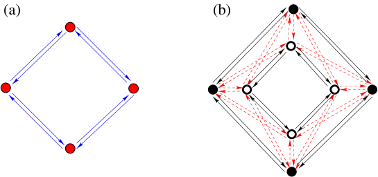
Figure 1: (a) Type II quiver diagram for the $\mathord{\!{\leavevmode\hbox{ \begin{picture}(0.6,0.7)\put(0.0,0.0){\line(1,0){0.6}} \put(0.0,0.75){\line(1,0){0.575}} \put(0.0,0.0){\rule{0.3pt}{0.3pt}}\put(0.0125,0.025){\rule{0.3pt}{0.3pt}}\put(0.025,0.05){\rule{0.3pt}{0.3pt}}\put(0.0375,0.075){\rule{0.3pt}{0.3pt}}\put(0.05,0.1){\rule{0.3pt}{0.3pt}}\put(0.0625,0.125){\rule{0.3pt}{0.3pt}}\put(0.075,0.15){\rule{0.3pt}{0.3pt}}\put(0.0875,0.175){\rule{0.3pt}{0.3pt}}\put(0.1,0.2){\rule{0.3pt}{0.3pt}}\put(0.1125,0.225){\rule{0.3pt}{0.3pt}}\put(0.125,0.25){\rule{0.3pt}{0.3pt}}\put(0.1375,0.275){\rule{0.3pt}{0.3pt}}\put(0.15,0.3){\rule{0.3pt}{0.3pt}}\put(0.1625,0.325){\rule{0.3pt}{0.3pt}}\put(0.175,0.35){\rule{0.3pt}{0.3pt}}\put(0.1875,0.375){\rule{0.3pt}{0.3pt}}\put(0.2,0.4){\rule{0.3pt}{0.3pt}}\put(0.2125,0.425){\rule{0.3pt}{0.3pt}}\put(0.225,0.45){\rule{0.3pt}{0.3pt}}\put(0.2375,0.475){\rule{0.3pt}{0.3pt}}\put(0.25,0.5){\rule{0.3pt}{0.3pt}}\put(0.2625,0.525){\rule{0.3pt}{0.3pt}}\put(0.275,0.55){\rule{0.3pt}{0.3pt}}\put(0.2875,0.575){\rule{0.3pt}{0.3pt}}\put(0.3,0.6){\rule{0.3pt}{0.3pt}}\put(0.3125,0.625){\rule{0.3pt}{0.3pt}}\put(0.325,0.65){\rule{0.3pt}{0.3pt}}\put(0.3375,0.675){\rule{0.3pt}{0.3pt}}\put(0.35,0.7){\rule{0.3pt}{0.3pt}}\put(0.3625,0.725){\rule{0.3pt}{0.3pt}} \put(0.2,0.0){\rule{0.3pt}{0.3pt}}\put(0.2125,0.025){\rule{0.3pt}{0.3pt}}\put(0.225,0.05){\rule{0.3pt}{0.3pt}}\put(0.2375,0.075){\rule{0.3pt}{0.3pt}}\put(0.25,0.1){\rule{0.3pt}{0.3pt}}\put(0.2625,0.125){\rule{0.3pt}{0.3pt}}\put(0.275,0.15){\rule{0.3pt}{0.3pt}}\put(0.2875,0.175){\rule{0.3pt}{0.3pt}}\put(0.3,0.2){\rule{0.3pt}{0.3pt}}\put(0.3125,0.225){\rule{0.3pt}{0.3pt}}\put(0.325,0.25){\rule{0.3pt}{0.3pt}}\put(0.3375,0.275){\rule{0.3pt}{0.3pt}}\put(0.35,0.3){\rule{0.3pt}{0.3pt}}\put(0.3625,0.325){\rule{0.3pt}{0.3pt}}\put(0.375,0.35){\rule{0.3pt}{0.3pt}}\put(0.3875,0.375){\rule{0.3pt}{0.3pt}}\put(0.4,0.4){\rule{0.3pt}{0.3pt}}\put(0.4125,0.425){\rule{0.3pt}{0.3pt}}\put(0.425,0.45){\rule{0.3pt}{0.3pt}}\put(0.4375,0.475){\rule{0.3pt}{0.3pt}}\put(0.45,0.5){\rule{0.3pt}{0.3pt}}\put(0.4625,0.525){\rule{0.3pt}{0.3pt}}\put(0.475,0.55){\rule{0.3pt}{0.3pt}}\put(0.4875,0.575){\rule{0.3pt}{0.3pt}}\put(0.5,0.6){\rule{0.3pt}{0.3pt}}\put(0.5125,0.625){\rule{0.3pt}{0.3pt}}\put(0.525,0.65){\rule{0.3pt}{0.3pt}}\put(0.5375,0.675){\rule{0.3pt}{0.3pt}}\put(0.55,0.7){\rule{0.3pt}{0.3pt}}\put(0.5625,0.725){\rule{0.3pt}{0.3pt}} \put(0.0,0.75){\line(0,-1){0.15}} \put(0.015,0.75){\line(0,-1){0.1}} \put(0.03,0.75){\line(0,-1){0.075}} \put(0.045,0.75){\line(0,-1){0.05}} \put(0.05,0.75){\line(0,-1){0.025}} \put(0.6,0.0){\line(0,1){0.15}} \put(0.585,0.0){\line(0,1){0.1}} \put(0.57,0.0){\line(0,1){0.075}} \put(0.555,0.0){\line(0,1){0.05}} \put(0.55,0.0){\line(0,1){0.025}} \end{picture}}}}_{4}$ orbifold. (b) Its type 0 counterpart: the links drawn with solid lines correspond to bosons, the other ones to fermions.

Next, let us consider the analogous situation for $N$ electric and $N$ magnetic type 0 D-branes. As discussed in Ref. [3] for the flat space case, one starts with $2N$ type II D-branes, derives the type II open string spectrum next, and finally performs a $(-)^{F_{\rm s}}\,{\cal I}$ projection to find the type 0 spectrum. $F_{\rm s}$ is the space-time fermion number and ${\cal I}$ acts as conjugation by $\sigma_{3}$ in the space of $N\times N$ blocks obtained by separating each group of $2N$ type II branes into $N$ electric and $N$ magnetic type 0 ones. The type 0 field content is as follows. The massless bosons are:

• 1 vector and 2 real scalars in the adjoint of each of the $n$ ${\rm SU}(N)\times{\rm SU}(N)$ factors of the gauge group;

• $n$ complex scalars, each in the representation $((N,1),(\bar{N},1))+((\bar{N},1),(N,1))$ of two ${\rm SU}(N)\times{\rm SU}(N)$ factors, as encoded in a type 0 quiver diagram, wich we will introduce shortly, see Fig. 1(b).

The massless fermionic content consists of:

• 2 Weyl fermions in the $(N,\bar{N})+(\bar{N},N)$ of each ${\rm SU}(N)\times{\rm SU}(N)$ group factor;

• $n$ Weyl fermions, each in the $((N,1),(1,\bar{N}))+((\bar{N},1),(1,N))$ of a couple of gauge factors as encoded in the type 0 diagram of Fig. 1(b).

The type 0 quiver diagram that summarizes the information about the spectrum requires only a slight modification of the quiver rules in Ref. [10]. For instance, in our $\mathord{\!{\leavevmode\hbox{ \begin{picture}(0.6,0.7)\put(0.0,0.0){\line(1,0){0.6}} \put(0.0,0.75){\line(1,0){0.575}} \put(0.0,0.0){\rule{0.3pt}{0.3pt}}\put(0.0125,0.025){\rule{0.3pt}{0.3pt}}\put(0.025,0.05){\rule{0.3pt}{0.3pt}}\put(0.0375,0.075){\rule{0.3pt}{0.3pt}}\put(0.05,0.1){\rule{0.3pt}{0.3pt}}\put(0.0625,0.125){\rule{0.3pt}{0.3pt}}\put(0.075,0.15){\rule{0.3pt}{0.3pt}}\put(0.0875,0.175){\rule{0.3pt}{0.3pt}}\put(0.1,0.2){\rule{0.3pt}{0.3pt}}\put(0.1125,0.225){\rule{0.3pt}{0.3pt}}\put(0.125,0.25){\rule{0.3pt}{0.3pt}}\put(0.1375,0.275){\rule{0.3pt}{0.3pt}}\put(0.15,0.3){\rule{0.3pt}{0.3pt}}\put(0.1625,0.325){\rule{0.3pt}{0.3pt}}\put(0.175,0.35){\rule{0.3pt}{0.3pt}}\put(0.1875,0.375){\rule{0.3pt}{0.3pt}}\put(0.2,0.4){\rule{0.3pt}{0.3pt}}\put(0.2125,0.425){\rule{0.3pt}{0.3pt}}\put(0.225,0.45){\rule{0.3pt}{0.3pt}}\put(0.2375,0.475){\rule{0.3pt}{0.3pt}}\put(0.25,0.5){\rule{0.3pt}{0.3pt}}\put(0.2625,0.525){\rule{0.3pt}{0.3pt}}\put(0.275,0.55){\rule{0.3pt}{0.3pt}}\put(0.2875,0.575){\rule{0.3pt}{0.3pt}}\put(0.3,0.6){\rule{0.3pt}{0.3pt}}\put(0.3125,0.625){\rule{0.3pt}{0.3pt}}\put(0.325,0.65){\rule{0.3pt}{0.3pt}}\put(0.3375,0.675){\rule{0.3pt}{0.3pt}}\put(0.35,0.7){\rule{0.3pt}{0.3pt}}\put(0.3625,0.725){\rule{0.3pt}{0.3pt}} \put(0.2,0.0){\rule{0.3pt}{0.3pt}}\put(0.2125,0.025){\rule{0.3pt}{0.3pt}}\put(0.225,0.05){\rule{0.3pt}{0.3pt}}\put(0.2375,0.075){\rule{0.3pt}{0.3pt}}\put(0.25,0.1){\rule{0.3pt}{0.3pt}}\put(0.2625,0.125){\rule{0.3pt}{0.3pt}}\put(0.275,0.15){\rule{0.3pt}{0.3pt}}\put(0.2875,0.175){\rule{0.3pt}{0.3pt}}\put(0.3,0.2){\rule{0.3pt}{0.3pt}}\put(0.3125,0.225){\rule{0.3pt}{0.3pt}}\put(0.325,0.25){\rule{0.3pt}{0.3pt}}\put(0.3375,0.275){\rule{0.3pt}{0.3pt}}\put(0.35,0.3){\rule{0.3pt}{0.3pt}}\put(0.3625,0.325){\rule{0.3pt}{0.3pt}}\put(0.375,0.35){\rule{0.3pt}{0.3pt}}\put(0.3875,0.375){\rule{0.3pt}{0.3pt}}\put(0.4,0.4){\rule{0.3pt}{0.3pt}}\put(0.4125,0.425){\rule{0.3pt}{0.3pt}}\put(0.425,0.45){\rule{0.3pt}{0.3pt}}\put(0.4375,0.475){\rule{0.3pt}{0.3pt}}\put(0.45,0.5){\rule{0.3pt}{0.3pt}}\put(0.4625,0.525){\rule{0.3pt}{0.3pt}}\put(0.475,0.55){\rule{0.3pt}{0.3pt}}\put(0.4875,0.575){\rule{0.3pt}{0.3pt}}\put(0.5,0.6){\rule{0.3pt}{0.3pt}}\put(0.5125,0.625){\rule{0.3pt}{0.3pt}}\put(0.525,0.65){\rule{0.3pt}{0.3pt}}\put(0.5375,0.675){\rule{0.3pt}{0.3pt}}\put(0.55,0.7){\rule{0.3pt}{0.3pt}}\put(0.5625,0.725){\rule{0.3pt}{0.3pt}} \put(0.0,0.75){\line(0,-1){0.15}} \put(0.015,0.75){\line(0,-1){0.1}} \put(0.03,0.75){\line(0,-1){0.075}} \put(0.045,0.75){\line(0,-1){0.05}} \put(0.05,0.75){\line(0,-1){0.025}} \put(0.6,0.0){\line(0,1){0.15}} \put(0.585,0.0){\line(0,1){0.1}} \put(0.57,0.0){\line(0,1){0.075}} \put(0.555,0.0){\line(0,1){0.05}} \put(0.55,0.0){\line(0,1){0.025}} \end{picture}}}}_{n}$ case, one draws $n$ pairs consisting of a filled and an empty dot, representing the groups of electric and magnetic branes, respectively; one then draws oriented links between any two dots inside one pair or in neighbouring pairs. The spectrum can be read off using the following rules:

1. every dot represents the bosonic content of an SU$(N)$ vector multiplet;

2. every link connecting two like dots corresponds to spacetime bosons;

3. every link between an empty and a filled dot corresponds to spacetime fermions;

4. a link represents the bosonic or fermionic truncation of either a vectormultiplet (in the case of links within a pair) or half a hypermultiplet (for links from one pair to a neighbouring one), transforming in the bifundamental of the gauge groups corresponding to the dots it connects.

4.1 Closed string description

As we saw in Section 2, in terms of unprojected R and NS boundary states one can with equal ease describe type II and type 0 D-branes. One can thus directly compute in the closed string channel the one-loop open string free energy that encodes the free spectrum of the gauge theory on the branes, both for type II and for type 0. We give now in some detail the closed-string description of the configuration treated above, namely D-branes sitting at an orbifold singularity (see also [23]); in particular, we will show how to incorporate the non-trivial action of the orbifold group on the Chan-Paton factors. As far as we know, this prescription is new, also in the type IIB context.

Let us thus consider D5-branes on $\mathord{\begin{picture}(0.6,0.7)(-0.1,0.0)\put(-0.1,0.0){\rm C} \put(0.2,0.05){\line(0,1){0.55}} \end{picture}}^{2}/\mathord{\!{\leavevmode\hbox{ \begin{picture}(0.6,0.7)\put(0.0,0.0){\line(1,0){0.6}} \put(0.0,0.75){\line(1,0){0.575}} \put(0.0,0.0){\rule{0.3pt}{0.3pt}}\put(0.0125,0.025){\rule{0.3pt}{0.3pt}}\put(0.025,0.05){\rule{0.3pt}{0.3pt}}\put(0.0375,0.075){\rule{0.3pt}{0.3pt}}\put(0.05,0.1){\rule{0.3pt}{0.3pt}}\put(0.0625,0.125){\rule{0.3pt}{0.3pt}}\put(0.075,0.15){\rule{0.3pt}{0.3pt}}\put(0.0875,0.175){\rule{0.3pt}{0.3pt}}\put(0.1,0.2){\rule{0.3pt}{0.3pt}}\put(0.1125,0.225){\rule{0.3pt}{0.3pt}}\put(0.125,0.25){\rule{0.3pt}{0.3pt}}\put(0.1375,0.275){\rule{0.3pt}{0.3pt}}\put(0.15,0.3){\rule{0.3pt}{0.3pt}}\put(0.1625,0.325){\rule{0.3pt}{0.3pt}}\put(0.175,0.35){\rule{0.3pt}{0.3pt}}\put(0.1875,0.375){\rule{0.3pt}{0.3pt}}\put(0.2,0.4){\rule{0.3pt}{0.3pt}}\put(0.2125,0.425){\rule{0.3pt}{0.3pt}}\put(0.225,0.45){\rule{0.3pt}{0.3pt}}\put(0.2375,0.475){\rule{0.3pt}{0.3pt}}\put(0.25,0.5){\rule{0.3pt}{0.3pt}}\put(0.2625,0.525){\rule{0.3pt}{0.3pt}}\put(0.275,0.55){\rule{0.3pt}{0.3pt}}\put(0.2875,0.575){\rule{0.3pt}{0.3pt}}\put(0.3,0.6){\rule{0.3pt}{0.3pt}}\put(0.3125,0.625){\rule{0.3pt}{0.3pt}}\put(0.325,0.65){\rule{0.3pt}{0.3pt}}\put(0.3375,0.675){\rule{0.3pt}{0.3pt}}\put(0.35,0.7){\rule{0.3pt}{0.3pt}}\put(0.3625,0.725){\rule{0.3pt}{0.3pt}} \put(0.2,0.0){\rule{0.3pt}{0.3pt}}\put(0.2125,0.025){\rule{0.3pt}{0.3pt}}\put(0.225,0.05){\rule{0.3pt}{0.3pt}}\put(0.2375,0.075){\rule{0.3pt}{0.3pt}}\put(0.25,0.1){\rule{0.3pt}{0.3pt}}\put(0.2625,0.125){\rule{0.3pt}{0.3pt}}\put(0.275,0.15){\rule{0.3pt}{0.3pt}}\put(0.2875,0.175){\rule{0.3pt}{0.3pt}}\put(0.3,0.2){\rule{0.3pt}{0.3pt}}\put(0.3125,0.225){\rule{0.3pt}{0.3pt}}\put(0.325,0.25){\rule{0.3pt}{0.3pt}}\put(0.3375,0.275){\rule{0.3pt}{0.3pt}}\put(0.35,0.3){\rule{0.3pt}{0.3pt}}\put(0.3625,0.325){\rule{0.3pt}{0.3pt}}\put(0.375,0.35){\rule{0.3pt}{0.3pt}}\put(0.3875,0.375){\rule{0.3pt}{0.3pt}}\put(0.4,0.4){\rule{0.3pt}{0.3pt}}\put(0.4125,0.425){\rule{0.3pt}{0.3pt}}\put(0.425,0.45){\rule{0.3pt}{0.3pt}}\put(0.4375,0.475){\rule{0.3pt}{0.3pt}}\put(0.45,0.5){\rule{0.3pt}{0.3pt}}\put(0.4625,0.525){\rule{0.3pt}{0.3pt}}\put(0.475,0.55){\rule{0.3pt}{0.3pt}}\put(0.4875,0.575){\rule{0.3pt}{0.3pt}}\put(0.5,0.6){\rule{0.3pt}{0.3pt}}\put(0.5125,0.625){\rule{0.3pt}{0.3pt}}\put(0.525,0.65){\rule{0.3pt}{0.3pt}}\put(0.5375,0.675){\rule{0.3pt}{0.3pt}}\put(0.55,0.7){\rule{0.3pt}{0.3pt}}\put(0.5625,0.725){\rule{0.3pt}{0.3pt}} \put(0.0,0.75){\line(0,-1){0.15}} \put(0.015,0.75){\line(0,-1){0.1}} \put(0.03,0.75){\line(0,-1){0.075}} \put(0.045,0.75){\line(0,-1){0.05}} \put(0.05,0.75){\line(0,-1){0.025}} \put(0.6,0.0){\line(0,1){0.15}} \put(0.585,0.0){\line(0,1){0.1}} \put(0.57,0.0){\line(0,1){0.075}} \put(0.555,0.0){\line(0,1){0.05}} \put(0.55,0.0){\line(0,1){0.025}} \end{picture}}}}_{n}$. The theory possesses $n$ closed string sectors, distinguished by the periodicity properties of the fields (see, e.g., Ref. [24]):

$$\{X,Y,\psi_{X},\psi_{Y}\}(\tau,\sigma+2\pi)=\{\omega^{l}X,\omega^{-l}Y,\omega^{l}\psi_{X},\omega^{-l}\psi_{Y}\}(\tau,\sigma)~{}.$$ (4.10)

Generically, the modings of the left and right moving oscillators, $\{\alpha_{\nu},\beta_{\lambda},\psi_{\nu},\chi_{\lambda}\}$ and $\{\tilde{\alpha}_{\tilde{\nu}},\tilde{\beta}_{\tilde{\lambda}},\tilde{\psi}_{\tilde{\nu}},\tilde{\chi}_{\tilde{\lambda}}\}$, are shifted from integer values: $\nu,\tilde{\lambda}\in\mathord{\!{\leavevmode\hbox{ \begin{picture}(0.6,0.7)\put(0.0,0.0){\line(1,0){0.6}} \put(0.0,0.75){\line(1,0){0.575}} \put(0.0,0.0){\rule{0.3pt}{0.3pt}}\put(0.0125,0.025){\rule{0.3pt}{0.3pt}}\put(0.025,0.05){\rule{0.3pt}{0.3pt}}\put(0.0375,0.075){\rule{0.3pt}{0.3pt}}\put(0.05,0.1){\rule{0.3pt}{0.3pt}}\put(0.0625,0.125){\rule{0.3pt}{0.3pt}}\put(0.075,0.15){\rule{0.3pt}{0.3pt}}\put(0.0875,0.175){\rule{0.3pt}{0.3pt}}\put(0.1,0.2){\rule{0.3pt}{0.3pt}}\put(0.1125,0.225){\rule{0.3pt}{0.3pt}}\put(0.125,0.25){\rule{0.3pt}{0.3pt}}\put(0.1375,0.275){\rule{0.3pt}{0.3pt}}\put(0.15,0.3){\rule{0.3pt}{0.3pt}}\put(0.1625,0.325){\rule{0.3pt}{0.3pt}}\put(0.175,0.35){\rule{0.3pt}{0.3pt}}\put(0.1875,0.375){\rule{0.3pt}{0.3pt}}\put(0.2,0.4){\rule{0.3pt}{0.3pt}}\put(0.2125,0.425){\rule{0.3pt}{0.3pt}}\put(0.225,0.45){\rule{0.3pt}{0.3pt}}\put(0.2375,0.475){\rule{0.3pt}{0.3pt}}\put(0.25,0.5){\rule{0.3pt}{0.3pt}}\put(0.2625,0.525){\rule{0.3pt}{0.3pt}}\put(0.275,0.55){\rule{0.3pt}{0.3pt}}\put(0.2875,0.575){\rule{0.3pt}{0.3pt}}\put(0.3,0.6){\rule{0.3pt}{0.3pt}}\put(0.3125,0.625){\rule{0.3pt}{0.3pt}}\put(0.325,0.65){\rule{0.3pt}{0.3pt}}\put(0.3375,0.675){\rule{0.3pt}{0.3pt}}\put(0.35,0.7){\rule{0.3pt}{0.3pt}}\put(0.3625,0.725){\rule{0.3pt}{0.3pt}} \put(0.2,0.0){\rule{0.3pt}{0.3pt}}\put(0.2125,0.025){\rule{0.3pt}{0.3pt}}\put(0.225,0.05){\rule{0.3pt}{0.3pt}}\put(0.2375,0.075){\rule{0.3pt}{0.3pt}}\put(0.25,0.1){\rule{0.3pt}{0.3pt}}\put(0.2625,0.125){\rule{0.3pt}{0.3pt}}\put(0.275,0.15){\rule{0.3pt}{0.3pt}}\put(0.2875,0.175){\rule{0.3pt}{0.3pt}}\put(0.3,0.2){\rule{0.3pt}{0.3pt}}\put(0.3125,0.225){\rule{0.3pt}{0.3pt}}\put(0.325,0.25){\rule{0.3pt}{0.3pt}}\put(0.3375,0.275){\rule{0.3pt}{0.3pt}}\put(0.35,0.3){\rule{0.3pt}{0.3pt}}\put(0.3625,0.325){\rule{0.3pt}{0.3pt}}\put(0.375,0.35){\rule{0.3pt}{0.3pt}}\put(0.3875,0.375){\rule{0.3pt}{0.3pt}}\put(0.4,0.4){\rule{0.3pt}{0.3pt}}\put(0.4125,0.425){\rule{0.3pt}{0.3pt}}\put(0.425,0.45){\rule{0.3pt}{0.3pt}}\put(0.4375,0.475){\rule{0.3pt}{0.3pt}}\put(0.45,0.5){\rule{0.3pt}{0.3pt}}\put(0.4625,0.525){\rule{0.3pt}{0.3pt}}\put(0.475,0.55){\rule{0.3pt}{0.3pt}}\put(0.4875,0.575){\rule{0.3pt}{0.3pt}}\put(0.5,0.6){\rule{0.3pt}{0.3pt}}\put(0.5125,0.625){\rule{0.3pt}{0.3pt}}\put(0.525,0.65){\rule{0.3pt}{0.3pt}}\put(0.5375,0.675){\rule{0.3pt}{0.3pt}}\put(0.55,0.7){\rule{0.3pt}{0.3pt}}\put(0.5625,0.725){\rule{0.3pt}{0.3pt}} \put(0.0,0.75){\line(0,-1){0.15}} \put(0.015,0.75){\line(0,-1){0.1}} \put(0.03,0.75){\line(0,-1){0.075}} \put(0.045,0.75){\line(0,-1){0.05}} \put(0.05,0.75){\line(0,-1){0.025}} \put(0.6,0.0){\line(0,1){0.15}} \put(0.585,0.0){\line(0,1){0.1}} \put(0.57,0.0){\line(0,1){0.075}} \put(0.555,0.0){\line(0,1){0.05}} \put(0.55,0.0){\line(0,1){0.025}} \end{picture}}}}+l/n$ and $\lambda,\tilde{\nu}\in\mathord{\!{\leavevmode\hbox{ \begin{picture}(0.6,0.7)\put(0.0,0.0){\line(1,0){0.6}} \put(0.0,0.75){\line(1,0){0.575}} \put(0.0,0.0){\rule{0.3pt}{0.3pt}}\put(0.0125,0.025){\rule{0.3pt}{0.3pt}}\put(0.025,0.05){\rule{0.3pt}{0.3pt}}\put(0.0375,0.075){\rule{0.3pt}{0.3pt}}\put(0.05,0.1){\rule{0.3pt}{0.3pt}}\put(0.0625,0.125){\rule{0.3pt}{0.3pt}}\put(0.075,0.15){\rule{0.3pt}{0.3pt}}\put(0.0875,0.175){\rule{0.3pt}{0.3pt}}\put(0.1,0.2){\rule{0.3pt}{0.3pt}}\put(0.1125,0.225){\rule{0.3pt}{0.3pt}}\put(0.125,0.25){\rule{0.3pt}{0.3pt}}\put(0.1375,0.275){\rule{0.3pt}{0.3pt}}\put(0.15,0.3){\rule{0.3pt}{0.3pt}}\put(0.1625,0.325){\rule{0.3pt}{0.3pt}}\put(0.175,0.35){\rule{0.3pt}{0.3pt}}\put(0.1875,0.375){\rule{0.3pt}{0.3pt}}\put(0.2,0.4){\rule{0.3pt}{0.3pt}}\put(0.2125,0.425){\rule{0.3pt}{0.3pt}}\put(0.225,0.45){\rule{0.3pt}{0.3pt}}\put(0.2375,0.475){\rule{0.3pt}{0.3pt}}\put(0.25,0.5){\rule{0.3pt}{0.3pt}}\put(0.2625,0.525){\rule{0.3pt}{0.3pt}}\put(0.275,0.55){\rule{0.3pt}{0.3pt}}\put(0.2875,0.575){\rule{0.3pt}{0.3pt}}\put(0.3,0.6){\rule{0.3pt}{0.3pt}}\put(0.3125,0.625){\rule{0.3pt}{0.3pt}}\put(0.325,0.65){\rule{0.3pt}{0.3pt}}\put(0.3375,0.675){\rule{0.3pt}{0.3pt}}\put(0.35,0.7){\rule{0.3pt}{0.3pt}}\put(0.3625,0.725){\rule{0.3pt}{0.3pt}} \put(0.2,0.0){\rule{0.3pt}{0.3pt}}\put(0.2125,0.025){\rule{0.3pt}{0.3pt}}\put(0.225,0.05){\rule{0.3pt}{0.3pt}}\put(0.2375,0.075){\rule{0.3pt}{0.3pt}}\put(0.25,0.1){\rule{0.3pt}{0.3pt}}\put(0.2625,0.125){\rule{0.3pt}{0.3pt}}\put(0.275,0.15){\rule{0.3pt}{0.3pt}}\put(0.2875,0.175){\rule{0.3pt}{0.3pt}}\put(0.3,0.2){\rule{0.3pt}{0.3pt}}\put(0.3125,0.225){\rule{0.3pt}{0.3pt}}\put(0.325,0.25){\rule{0.3pt}{0.3pt}}\put(0.3375,0.275){\rule{0.3pt}{0.3pt}}\put(0.35,0.3){\rule{0.3pt}{0.3pt}}\put(0.3625,0.325){\rule{0.3pt}{0.3pt}}\put(0.375,0.35){\rule{0.3pt}{0.3pt}}\put(0.3875,0.375){\rule{0.3pt}{0.3pt}}\put(0.4,0.4){\rule{0.3pt}{0.3pt}}\put(0.4125,0.425){\rule{0.3pt}{0.3pt}}\put(0.425,0.45){\rule{0.3pt}{0.3pt}}\put(0.4375,0.475){\rule{0.3pt}{0.3pt}}\put(0.45,0.5){\rule{0.3pt}{0.3pt}}\put(0.4625,0.525){\rule{0.3pt}{0.3pt}}\put(0.475,0.55){\rule{0.3pt}{0.3pt}}\put(0.4875,0.575){\rule{0.3pt}{0.3pt}}\put(0.5,0.6){\rule{0.3pt}{0.3pt}}\put(0.5125,0.625){\rule{0.3pt}{0.3pt}}\put(0.525,0.65){\rule{0.3pt}{0.3pt}}\put(0.5375,0.675){\rule{0.3pt}{0.3pt}}\put(0.55,0.7){\rule{0.3pt}{0.3pt}}\put(0.5625,0.725){\rule{0.3pt}{0.3pt}} \put(0.0,0.75){\line(0,-1){0.15}} \put(0.015,0.75){\line(0,-1){0.1}} \put(0.03,0.75){\line(0,-1){0.075}} \put(0.045,0.75){\line(0,-1){0.05}} \put(0.05,0.75){\line(0,-1){0.025}} \put(0.6,0.0){\line(0,1){0.15}} \put(0.585,0.0){\line(0,1){0.1}} \put(0.57,0.0){\line(0,1){0.075}} \put(0.555,0.0){\line(0,1){0.05}} \put(0.55,0.0){\line(0,1){0.025}} \end{picture}}}}-l/n$ (plus of course an additional shift of 1/2 for the fermionic oscillators in the NS sector). In the following we give explicit expressions for the $X$ and $\psi_{X}$ parts only.

A D5-brane localized at the orbifold fixed point is represented in the $l$-th twisted sector by a boundary state that satisfies

$$(X^{(l)}\,+\,\tilde{X}^{(l)})|_{\tau=0}|{B;l}\rangle=0~{},\hskip 8.5359pt(\psi^{(l)}\,+\,{\rm i}\eta\,\tilde{\psi}^{(l)})|_{\tau=0}|{B;l}\rangle=0~{},$$ (4.11)

plus conjugate relations and plus appropriate counterparts on $Y,\bar{Y}$ and $\psi_{Y},\bar{\psi}_{Y}$.

The solution to these conditions in terms of oscillators is, writing $|{B;l}\rangle$ as the product $|{B_{\rm b};l}\rangle\otimes|{B_{\rm f},\eta;l}\rangle_{\rm R,NS}$ of a bosonic and a fermionic part,

$$|{B_{\rm b};l}\rangle = \exp\Bigl{(}\sum_{\nu}\,{\bar{\alpha}_{-\nu}\tilde{\alpha}_{-\nu}\over\nu}+\,\sum_{\bar{\nu}}{\alpha_{-\bar{\nu}}\tilde{\bar{\alpha}}_{-\bar{\nu}}\over\bar{\nu}}\Bigr{)}|{0}\rangle~{},$$

$$|{B_{\rm f},\eta;l}\rangle_{\rm R,NS} = \exp\Bigl{(}-{\rm i}\eta\,\sum_{\nu}\,\bar{\psi}_{-\nu}\tilde{\psi}_{-\nu}-{\rm i}\eta\,\sum_{\bar{\nu}}\psi_{-\bar{\nu}}\tilde{\bar{\psi}}_{-\bar{\nu}}\Bigr{)}|{0}\rangle~{},$$ (4.12)

where the modings are as indicated below Eq. (4.10) and, as usual, the fermionic part of the boundary state depends on the additional sign $\eta$.

Suppose now to have $nN$ D-branes, which for our purposes we can represent by $nN$ boundary states, labeled by “Chan-Paton” indices. In the case we are interested in, we group the D5-branes into $n$ bunches and use a Chan-Paton composite label $i,A$, with $i=0,\ldots,n$ and $A=1,\ldots,N$. In the type 0 context, we start with $A=1,\ldots,2N$ and we split it into $a=1,\ldots,N$, for the $N$ electric branes and $\bar{a}=1,\ldots,N$ for the magnetic ones.

The cylinder amplitude between any two given D-branes, i.e., for fixed Chan-Paton indices, receives contributions from all the twisted sectors. In summing the twisted sectors, an ambiguity shows up: for each Chan-Paton label we can independently decide how to weigh the twisted sectors. This is the closed string counterpart of the freedom one has in the open string picture to introduce a non-trivial action of the orbifold group on the adjoint Chan-Paton factor. In the $\mathord{\begin{picture}(0.6,0.7)(-0.1,0.0)\put(-0.1,0.0){\rm C} \put(0.2,0.05){\line(0,1){0.55}} \end{picture}}^{2}/\mathord{\!{\leavevmode\hbox{ \begin{picture}(0.6,0.7)\put(0.0,0.0){\line(1,0){0.6}} \put(0.0,0.75){\line(1,0){0.575}} \put(0.0,0.0){\rule{0.3pt}{0.3pt}}\put(0.0125,0.025){\rule{0.3pt}{0.3pt}}\put(0.025,0.05){\rule{0.3pt}{0.3pt}}\put(0.0375,0.075){\rule{0.3pt}{0.3pt}}\put(0.05,0.1){\rule{0.3pt}{0.3pt}}\put(0.0625,0.125){\rule{0.3pt}{0.3pt}}\put(0.075,0.15){\rule{0.3pt}{0.3pt}}\put(0.0875,0.175){\rule{0.3pt}{0.3pt}}\put(0.1,0.2){\rule{0.3pt}{0.3pt}}\put(0.1125,0.225){\rule{0.3pt}{0.3pt}}\put(0.125,0.25){\rule{0.3pt}{0.3pt}}\put(0.1375,0.275){\rule{0.3pt}{0.3pt}}\put(0.15,0.3){\rule{0.3pt}{0.3pt}}\put(0.1625,0.325){\rule{0.3pt}{0.3pt}}\put(0.175,0.35){\rule{0.3pt}{0.3pt}}\put(0.1875,0.375){\rule{0.3pt}{0.3pt}}\put(0.2,0.4){\rule{0.3pt}{0.3pt}}\put(0.2125,0.425){\rule{0.3pt}{0.3pt}}\put(0.225,0.45){\rule{0.3pt}{0.3pt}}\put(0.2375,0.475){\rule{0.3pt}{0.3pt}}\put(0.25,0.5){\rule{0.3pt}{0.3pt}}\put(0.2625,0.525){\rule{0.3pt}{0.3pt}}\put(0.275,0.55){\rule{0.3pt}{0.3pt}}\put(0.2875,0.575){\rule{0.3pt}{0.3pt}}\put(0.3,0.6){\rule{0.3pt}{0.3pt}}\put(0.3125,0.625){\rule{0.3pt}{0.3pt}}\put(0.325,0.65){\rule{0.3pt}{0.3pt}}\put(0.3375,0.675){\rule{0.3pt}{0.3pt}}\put(0.35,0.7){\rule{0.3pt}{0.3pt}}\put(0.3625,0.725){\rule{0.3pt}{0.3pt}} \put(0.2,0.0){\rule{0.3pt}{0.3pt}}\put(0.2125,0.025){\rule{0.3pt}{0.3pt}}\put(0.225,0.05){\rule{0.3pt}{0.3pt}}\put(0.2375,0.075){\rule{0.3pt}{0.3pt}}\put(0.25,0.1){\rule{0.3pt}{0.3pt}}\put(0.2625,0.125){\rule{0.3pt}{0.3pt}}\put(0.275,0.15){\rule{0.3pt}{0.3pt}}\put(0.2875,0.175){\rule{0.3pt}{0.3pt}}\put(0.3,0.2){\rule{0.3pt}{0.3pt}}\put(0.3125,0.225){\rule{0.3pt}{0.3pt}}\put(0.325,0.25){\rule{0.3pt}{0.3pt}}\put(0.3375,0.275){\rule{0.3pt}{0.3pt}}\put(0.35,0.3){\rule{0.3pt}{0.3pt}}\put(0.3625,0.325){\rule{0.3pt}{0.3pt}}\put(0.375,0.35){\rule{0.3pt}{0.3pt}}\put(0.3875,0.375){\rule{0.3pt}{0.3pt}}\put(0.4,0.4){\rule{0.3pt}{0.3pt}}\put(0.4125,0.425){\rule{0.3pt}{0.3pt}}\put(0.425,0.45){\rule{0.3pt}{0.3pt}}\put(0.4375,0.475){\rule{0.3pt}{0.3pt}}\put(0.45,0.5){\rule{0.3pt}{0.3pt}}\put(0.4625,0.525){\rule{0.3pt}{0.3pt}}\put(0.475,0.55){\rule{0.3pt}{0.3pt}}\put(0.4875,0.575){\rule{0.3pt}{0.3pt}}\put(0.5,0.6){\rule{0.3pt}{0.3pt}}\put(0.5125,0.625){\rule{0.3pt}{0.3pt}}\put(0.525,0.65){\rule{0.3pt}{0.3pt}}\put(0.5375,0.675){\rule{0.3pt}{0.3pt}}\put(0.55,0.7){\rule{0.3pt}{0.3pt}}\put(0.5625,0.725){\rule{0.3pt}{0.3pt}} \put(0.0,0.75){\line(0,-1){0.15}} \put(0.015,0.75){\line(0,-1){0.1}} \put(0.03,0.75){\line(0,-1){0.075}} \put(0.045,0.75){\line(0,-1){0.05}} \put(0.05,0.75){\line(0,-1){0.025}} \put(0.6,0.0){\line(0,1){0.15}} \put(0.585,0.0){\line(0,1){0.1}} \put(0.57,0.0){\line(0,1){0.075}} \put(0.555,0.0){\line(0,1){0.05}} \put(0.55,0.0){\line(0,1){0.025}} \end{picture}}}}_{n}$ case, the regular action $(i,a;j,b)\to\omega^{i-j}(i,a;j,b)$ of the orbifold generator described at the beginning of Section 4 is reproduced in the closed string language by defining the cylinder amplitude to be

$$({\cal A}^{ij})^{ab}=\sum_{l=0}^{n-1}\omega^{l(i-j)}\,\langle{B,\eta^{\prime};l;i,a}|D|{B,\eta;l;j,b}\rangle~{},$$ (4.13)

where $D$ is the closed string propagator and of course the R or NS fermions must be distinguished. Explicitly, the amplitude (4.13) turns out to be

$$({\cal A}_{\gamma}^{ij})^{ab}={\rm i}V_{6}(-)^{\delta_{\gamma,2}}(8\pi^{2}\alpha^{\prime})^{-3}\int_{0}^{-{\rm i}\infty}d\tau\,{1\over n}\sum_{l=0}^{n-1}\omega^{l(i-j)}\,c_{l}\,\left({f_{\gamma}(\tau)\over f_{1}(\tau)}\right)^{4}\left({\theta_{\gamma}(\tau l/n|\tau)\over\theta_{1}(\tau l/n|\tau)}\right)^{2}~{},$$ (4.14)

where $V_{6}$ is the 5-brane volume, $c_{0}=1$ and $c_{l}=4\sin^{2}(\pi l/n)$ for $l>0$ and we have $\gamma=2$ for the R-R sector with $\eta^{\prime}\eta=-1$, $\gamma=3$ for the NS-NS sector with $\eta^{\prime}\eta=-1$ and $\gamma=4$ for the NS-NS sector with $\eta^{\prime}\eta=1$. The R-R amplitude with $\eta^{\prime}\eta=1$ vanishes. In Eq. (4.14) we have used also the expressions $f_{\gamma}(\tau)$ of Ref. [25].

The modular transformation of the amplitude (4.14) allows one to recognize it as a 1-loop open string free energy. In terms of $\tau^{\prime}=-1/\tau$, $({\cal A}_{\gamma}^{ij})^{ab}$ is rewritten as

$$({\tilde{\cal A}}_{\gamma^{\prime}}^{ij})^{ab}=-{\rm i}V_{6}(-)^{\delta_{\gamma^{\prime},4}}\int_{0}^{{\rm i}\infty}d\tau^{\prime}(8\pi^{2}\alpha^{\prime})^{-3}{1\over n}\sum_{l=0}^{n-1}\omega^{l(i-j)}\,c_{l}\,\left({f_{\gamma^{\prime}}(\tau^{\prime})\over f_{1}(\tau^{\prime})}\right)^{4}\left({\theta_{\gamma^{\prime}}(l/n|\tau^{\prime})\over\theta_{1}(l/n|\tau^{\prime})}\right)^{2}~{},$$ (4.15)

with $2^{\prime}=4$, $3^{\prime}=3$ and $4^{\prime}=2$. The full amplitude ${\tilde{\cal A}}_{\gamma^{\prime}}$, obtained summing over all adjoint Chan-Paton indices, coincides with the 1-loop free energy for the $\mathord{\!{\leavevmode\hbox{ \begin{picture}(0.6,0.7)\put(0.0,0.0){\line(1,0){0.6}} \put(0.0,0.75){\line(1,0){0.575}} \put(0.0,0.0){\rule{0.3pt}{0.3pt}}\put(0.0125,0.025){\rule{0.3pt}{0.3pt}}\put(0.025,0.05){\rule{0.3pt}{0.3pt}}\put(0.0375,0.075){\rule{0.3pt}{0.3pt}}\put(0.05,0.1){\rule{0.3pt}{0.3pt}}\put(0.0625,0.125){\rule{0.3pt}{0.3pt}}\put(0.075,0.15){\rule{0.3pt}{0.3pt}}\put(0.0875,0.175){\rule{0.3pt}{0.3pt}}\put(0.1,0.2){\rule{0.3pt}{0.3pt}}\put(0.1125,0.225){\rule{0.3pt}{0.3pt}}\put(0.125,0.25){\rule{0.3pt}{0.3pt}}\put(0.1375,0.275){\rule{0.3pt}{0.3pt}}\put(0.15,0.3){\rule{0.3pt}{0.3pt}}\put(0.1625,0.325){\rule{0.3pt}{0.3pt}}\put(0.175,0.35){\rule{0.3pt}{0.3pt}}\put(0.1875,0.375){\rule{0.3pt}{0.3pt}}\put(0.2,0.4){\rule{0.3pt}{0.3pt}}\put(0.2125,0.425){\rule{0.3pt}{0.3pt}}\put(0.225,0.45){\rule{0.3pt}{0.3pt}}\put(0.2375,0.475){\rule{0.3pt}{0.3pt}}\put(0.25,0.5){\rule{0.3pt}{0.3pt}}\put(0.2625,0.525){\rule{0.3pt}{0.3pt}}\put(0.275,0.55){\rule{0.3pt}{0.3pt}}\put(0.2875,0.575){\rule{0.3pt}{0.3pt}}\put(0.3,0.6){\rule{0.3pt}{0.3pt}}\put(0.3125,0.625){\rule{0.3pt}{0.3pt}}\put(0.325,0.65){\rule{0.3pt}{0.3pt}}\put(0.3375,0.675){\rule{0.3pt}{0.3pt}}\put(0.35,0.7){\rule{0.3pt}{0.3pt}}\put(0.3625,0.725){\rule{0.3pt}{0.3pt}} \put(0.2,0.0){\rule{0.3pt}{0.3pt}}\put(0.2125,0.025){\rule{0.3pt}{0.3pt}}\put(0.225,0.05){\rule{0.3pt}{0.3pt}}\put(0.2375,0.075){\rule{0.3pt}{0.3pt}}\put(0.25,0.1){\rule{0.3pt}{0.3pt}}\put(0.2625,0.125){\rule{0.3pt}{0.3pt}}\put(0.275,0.15){\rule{0.3pt}{0.3pt}}\put(0.2875,0.175){\rule{0.3pt}{0.3pt}}\put(0.3,0.2){\rule{0.3pt}{0.3pt}}\put(0.3125,0.225){\rule{0.3pt}{0.3pt}}\put(0.325,0.25){\rule{0.3pt}{0.3pt}}\put(0.3375,0.275){\rule{0.3pt}{0.3pt}}\put(0.35,0.3){\rule{0.3pt}{0.3pt}}\put(0.3625,0.325){\rule{0.3pt}{0.3pt}}\put(0.375,0.35){\rule{0.3pt}{0.3pt}}\put(0.3875,0.375){\rule{0.3pt}{0.3pt}}\put(0.4,0.4){\rule{0.3pt}{0.3pt}}\put(0.4125,0.425){\rule{0.3pt}{0.3pt}}\put(0.425,0.45){\rule{0.3pt}{0.3pt}}\put(0.4375,0.475){\rule{0.3pt}{0.3pt}}\put(0.45,0.5){\rule{0.3pt}{0.3pt}}\put(0.4625,0.525){\rule{0.3pt}{0.3pt}}\put(0.475,0.55){\rule{0.3pt}{0.3pt}}\put(0.4875,0.575){\rule{0.3pt}{0.3pt}}\put(0.5,0.6){\rule{0.3pt}{0.3pt}}\put(0.5125,0.625){\rule{0.3pt}{0.3pt}}\put(0.525,0.65){\rule{0.3pt}{0.3pt}}\put(0.5375,0.675){\rule{0.3pt}{0.3pt}}\put(0.55,0.7){\rule{0.3pt}{0.3pt}}\put(0.5625,0.725){\rule{0.3pt}{0.3pt}} \put(0.0,0.75){\line(0,-1){0.15}} \put(0.015,0.75){\line(0,-1){0.1}} \put(0.03,0.75){\line(0,-1){0.075}} \put(0.045,0.75){\line(0,-1){0.05}} \put(0.05,0.75){\line(0,-1){0.025}} \put(0.6,0.0){\line(0,1){0.15}} \put(0.585,0.0){\line(0,1){0.1}} \put(0.57,0.0){\line(0,1){0.075}} \put(0.555,0.0){\line(0,1){0.05}} \put(0.55,0.0){\line(0,1){0.025}} \end{picture}}}}_{n}$-invariant states of the open strings attached to the D5-branes:

$$V_{6}\int{d^{6}k\over(2\pi)^{6}}\int_{0}^{{\rm i}\infty}{d\tau^{\prime}\over\tau^{\prime}}\,{\rm Tr}_{\gamma^{\prime}}\left\{{\rm e}^{2\pi{\rm i}\tau^{\prime}(L_{0}-a)}\,{\cal P}\right\}~{},$$ (4.16)

where the trace runs over the adjoint Chan-Paton indices and over the Hilbert space generated by the open string oscillators. ${\cal P}$ denotes the projector $\frac{1}{n}\sum_{l=0}^{n-1}\hat{\omega}^{l}$, with $\hat{\omega}$ realizing on the open string states the $\mathord{\!{\leavevmode\hbox{ \begin{picture}(0.6,0.7)\put(0.0,0.0){\line(1,0){0.6}} \put(0.0,0.75){\line(1,0){0.575}} \put(0.0,0.0){\rule{0.3pt}{0.3pt}}\put(0.0125,0.025){\rule{0.3pt}{0.3pt}}\put(0.025,0.05){\rule{0.3pt}{0.3pt}}\put(0.0375,0.075){\rule{0.3pt}{0.3pt}}\put(0.05,0.1){\rule{0.3pt}{0.3pt}}\put(0.0625,0.125){\rule{0.3pt}{0.3pt}}\put(0.075,0.15){\rule{0.3pt}{0.3pt}}\put(0.0875,0.175){\rule{0.3pt}{0.3pt}}\put(0.1,0.2){\rule{0.3pt}{0.3pt}}\put(0.1125,0.225){\rule{0.3pt}{0.3pt}}\put(0.125,0.25){\rule{0.3pt}{0.3pt}}\put(0.1375,0.275){\rule{0.3pt}{0.3pt}}\put(0.15,0.3){\rule{0.3pt}{0.3pt}}\put(0.1625,0.325){\rule{0.3pt}{0.3pt}}\put(0.175,0.35){\rule{0.3pt}{0.3pt}}\put(0.1875,0.375){\rule{0.3pt}{0.3pt}}\put(0.2,0.4){\rule{0.3pt}{0.3pt}}\put(0.2125,0.425){\rule{0.3pt}{0.3pt}}\put(0.225,0.45){\rule{0.3pt}{0.3pt}}\put(0.2375,0.475){\rule{0.3pt}{0.3pt}}\put(0.25,0.5){\rule{0.3pt}{0.3pt}}\put(0.2625,0.525){\rule{0.3pt}{0.3pt}}\put(0.275,0.55){\rule{0.3pt}{0.3pt}}\put(0.2875,0.575){\rule{0.3pt}{0.3pt}}\put(0.3,0.6){\rule{0.3pt}{0.3pt}}\put(0.3125,0.625){\rule{0.3pt}{0.3pt}}\put(0.325,0.65){\rule{0.3pt}{0.3pt}}\put(0.3375,0.675){\rule{0.3pt}{0.3pt}}\put(0.35,0.7){\rule{0.3pt}{0.3pt}}\put(0.3625,0.725){\rule{0.3pt}{0.3pt}} \put(0.2,0.0){\rule{0.3pt}{0.3pt}}\put(0.2125,0.025){\rule{0.3pt}{0.3pt}}\put(0.225,0.05){\rule{0.3pt}{0.3pt}}\put(0.2375,0.075){\rule{0.3pt}{0.3pt}}\put(0.25,0.1){\rule{0.3pt}{0.3pt}}\put(0.2625,0.125){\rule{0.3pt}{0.3pt}}\put(0.275,0.15){\rule{0.3pt}{0.3pt}}\put(0.2875,0.175){\rule{0.3pt}{0.3pt}}\put(0.3,0.2){\rule{0.3pt}{0.3pt}}\put(0.3125,0.225){\rule{0.3pt}{0.3pt}}\put(0.325,0.25){\rule{0.3pt}{0.3pt}}\put(0.3375,0.275){\rule{0.3pt}{0.3pt}}\put(0.35,0.3){\rule{0.3pt}{0.3pt}}\put(0.3625,0.325){\rule{0.3pt}{0.3pt}}\put(0.375,0.35){\rule{0.3pt}{0.3pt}}\put(0.3875,0.375){\rule{0.3pt}{0.3pt}}\put(0.4,0.4){\rule{0.3pt}{0.3pt}}\put(0.4125,0.425){\rule{0.3pt}{0.3pt}}\put(0.425,0.45){\rule{0.3pt}{0.3pt}}\put(0.4375,0.475){\rule{0.3pt}{0.3pt}}\put(0.45,0.5){\rule{0.3pt}{0.3pt}}\put(0.4625,0.525){\rule{0.3pt}{0.3pt}}\put(0.475,0.55){\rule{0.3pt}{0.3pt}}\put(0.4875,0.575){\rule{0.3pt}{0.3pt}}\put(0.5,0.6){\rule{0.3pt}{0.3pt}}\put(0.5125,0.625){\rule{0.3pt}{0.3pt}}\put(0.525,0.65){\rule{0.3pt}{0.3pt}}\put(0.5375,0.675){\rule{0.3pt}{0.3pt}}\put(0.55,0.7){\rule{0.3pt}{0.3pt}}\put(0.5625,0.725){\rule{0.3pt}{0.3pt}} \put(0.0,0.75){\line(0,-1){0.15}} \put(0.015,0.75){\line(0,-1){0.1}} \put(0.03,0.75){\line(0,-1){0.075}} \put(0.045,0.75){\line(0,-1){0.05}} \put(0.05,0.75){\line(0,-1){0.025}} \put(0.6,0.0){\line(0,1){0.15}} \put(0.585,0.0){\line(0,1){0.1}} \put(0.57,0.0){\line(0,1){0.075}} \put(0.555,0.0){\line(0,1){0.05}} \put(0.55,0.0){\line(0,1){0.025}} \end{picture}}}}_{n}$ generator.

From the various “building blocks” (4.15) we construct the type II and type 0 expressions by taking the combinations required by the definitions (2.3) and (2.4), respectively. In the type II case, we get $\frac{1}{2}({\tilde{\cal A}}^{ij}_{3}-{\tilde{\cal A}}^{ij}_{4}-{\tilde{\cal A}}^{ij}_{2})^{ab}$. In type 0, we must make the following distinction: for electric-electric or magnetic-magnetic interactions ($ab$ or $\bar{a}\bar{b}$ indices), where $\eta\eta^{\prime}=-1$, we get only contributions from the open string NS sector: $\frac{1}{2}({\tilde{\cal A}}^{ij}_{3}-{\tilde{\cal A}}^{ij}_{4})^{ab}$; for electric-magnetic ones, where $\eta\eta^{\prime}=1$, only the R sector (i.e. worldvolume fermions) contributes: $-\frac{1}{2}({\tilde{\cal A}}^{ij}_{2})^{a\bar{b}}$. Expanding the integrands of these expressions in powers of ${\rm e}^{\pi{\rm i}\tau^{\prime}}$ we can count the on-shell states in the world-volume theory that carry given Chan-Paton indices, at the various mass levels. In particular, the only massless contributions arise when $|i-j|$ equals 0 or 1, and the spectrum of the gauge theory on the world-volume is seen to coincide with the one described in the previous section.

4.2 Large N conformal invariance

According to a general argument [9], large $N$ conformal invariance, whence a vanishing beta function in the large $N$ limit, is to be expected for the gauge theory on the branes at the orbifold singularity. Let us first review the basic ingredients of this argument. Starting from a parent ${\cal N}=4$ theory, one can build a new theory by taking the orbifold with respect to a discrete subgroup $\Gamma$ of the SU(4)_R ${\cal R}$-symmetry group. If every non-trivial $g\in\Gamma$ acts on a (fundamental) Chan-Paton index as a traceless matrix $\gamma_{g}$, the large $N$ vanishing of the beta function in the orbifold theory can be demonstrated to all orders. According to Ref. [9] this condition on the action of $\Gamma$ amounts to imposing that the Chan-Paton indices transform in a number of copies of the regular representation of $\Gamma$.

Let us now take the concrete example of $N$ electric and $N$ magnetic type 0 D3 branes at a $\mathord{\begin{picture}(0.6,0.7)(-0.1,0.0)\put(-0.1,0.0){\rm C} \put(0.2,0.05){\line(0,1){0.55}} \end{picture}}^{2}/\mathord{\!{\leavevmode\hbox{ \begin{picture}(0.6,0.7)\put(0.0,0.0){\line(1,0){0.6}} \put(0.0,0.75){\line(1,0){0.575}} \put(0.0,0.0){\rule{0.3pt}{0.3pt}}\put(0.0125,0.025){\rule{0.3pt}{0.3pt}}\put(0.025,0.05){\rule{0.3pt}{0.3pt}}\put(0.0375,0.075){\rule{0.3pt}{0.3pt}}\put(0.05,0.1){\rule{0.3pt}{0.3pt}}\put(0.0625,0.125){\rule{0.3pt}{0.3pt}}\put(0.075,0.15){\rule{0.3pt}{0.3pt}}\put(0.0875,0.175){\rule{0.3pt}{0.3pt}}\put(0.1,0.2){\rule{0.3pt}{0.3pt}}\put(0.1125,0.225){\rule{0.3pt}{0.3pt}}\put(0.125,0.25){\rule{0.3pt}{0.3pt}}\put(0.1375,0.275){\rule{0.3pt}{0.3pt}}\put(0.15,0.3){\rule{0.3pt}{0.3pt}}\put(0.1625,0.325){\rule{0.3pt}{0.3pt}}\put(0.175,0.35){\rule{0.3pt}{0.3pt}}\put(0.1875,0.375){\rule{0.3pt}{0.3pt}}\put(0.2,0.4){\rule{0.3pt}{0.3pt}}\put(0.2125,0.425){\rule{0.3pt}{0.3pt}}\put(0.225,0.45){\rule{0.3pt}{0.3pt}}\put(0.2375,0.475){\rule{0.3pt}{0.3pt}}\put(0.25,0.5){\rule{0.3pt}{0.3pt}}\put(0.2625,0.525){\rule{0.3pt}{0.3pt}}\put(0.275,0.55){\rule{0.3pt}{0.3pt}}\put(0.2875,0.575){\rule{0.3pt}{0.3pt}}\put(0.3,0.6){\rule{0.3pt}{0.3pt}}\put(0.3125,0.625){\rule{0.3pt}{0.3pt}}\put(0.325,0.65){\rule{0.3pt}{0.3pt}}\put(0.3375,0.675){\rule{0.3pt}{0.3pt}}\put(0.35,0.7){\rule{0.3pt}{0.3pt}}\put(0.3625,0.725){\rule{0.3pt}{0.3pt}} \put(0.2,0.0){\rule{0.3pt}{0.3pt}}\put(0.2125,0.025){\rule{0.3pt}{0.3pt}}\put(0.225,0.05){\rule{0.3pt}{0.3pt}}\put(0.2375,0.075){\rule{0.3pt}{0.3pt}}\put(0.25,0.1){\rule{0.3pt}{0.3pt}}\put(0.2625,0.125){\rule{0.3pt}{0.3pt}}\put(0.275,0.15){\rule{0.3pt}{0.3pt}}\put(0.2875,0.175){\rule{0.3pt}{0.3pt}}\put(0.3,0.2){\rule{0.3pt}{0.3pt}}\put(0.3125,0.225){\rule{0.3pt}{0.3pt}}\put(0.325,0.25){\rule{0.3pt}{0.3pt}}\put(0.3375,0.275){\rule{0.3pt}{0.3pt}}\put(0.35,0.3){\rule{0.3pt}{0.3pt}}\put(0.3625,0.325){\rule{0.3pt}{0.3pt}}\put(0.375,0.35){\rule{0.3pt}{0.3pt}}\put(0.3875,0.375){\rule{0.3pt}{0.3pt}}\put(0.4,0.4){\rule{0.3pt}{0.3pt}}\put(0.4125,0.425){\rule{0.3pt}{0.3pt}}\put(0.425,0.45){\rule{0.3pt}{0.3pt}}\put(0.4375,0.475){\rule{0.3pt}{0.3pt}}\put(0.45,0.5){\rule{0.3pt}{0.3pt}}\put(0.4625,0.525){\rule{0.3pt}{0.3pt}}\put(0.475,0.55){\rule{0.3pt}{0.3pt}}\put(0.4875,0.575){\rule{0.3pt}{0.3pt}}\put(0.5,0.6){\rule{0.3pt}{0.3pt}}\put(0.5125,0.625){\rule{0.3pt}{0.3pt}}\put(0.525,0.65){\rule{0.3pt}{0.3pt}}\put(0.5375,0.675){\rule{0.3pt}{0.3pt}}\put(0.55,0.7){\rule{0.3pt}{0.3pt}}\put(0.5625,0.725){\rule{0.3pt}{0.3pt}} \put(0.0,0.75){\line(0,-1){0.15}} \put(0.015,0.75){\line(0,-1){0.1}} \put(0.03,0.75){\line(0,-1){0.075}} \put(0.045,0.75){\line(0,-1){0.05}} \put(0.05,0.75){\line(0,-1){0.025}} \put(0.6,0.0){\line(0,1){0.15}} \put(0.585,0.0){\line(0,1){0.1}} \put(0.57,0.0){\line(0,1){0.075}} \put(0.555,0.0){\line(0,1){0.05}} \put(0.55,0.0){\line(0,1){0.025}} \end{picture}}}}_{n}$ singularity. Starting from the U($2nN$) ${\cal N}=4$ gauge theory corresponding to $2nN$ type II branes in flat spaces, the type 0 worldvolume theory is obtained by orbifolding with $\mathord{\!{\leavevmode\hbox{ \begin{picture}(0.6,0.7)\put(0.0,0.0){\line(1,0){0.6}} \put(0.0,0.75){\line(1,0){0.575}} \put(0.0,0.0){\rule{0.3pt}{0.3pt}}\put(0.0125,0.025){\rule{0.3pt}{0.3pt}}\put(0.025,0.05){\rule{0.3pt}{0.3pt}}\put(0.0375,0.075){\rule{0.3pt}{0.3pt}}\put(0.05,0.1){\rule{0.3pt}{0.3pt}}\put(0.0625,0.125){\rule{0.3pt}{0.3pt}}\put(0.075,0.15){\rule{0.3pt}{0.3pt}}\put(0.0875,0.175){\rule{0.3pt}{0.3pt}}\put(0.1,0.2){\rule{0.3pt}{0.3pt}}\put(0.1125,0.225){\rule{0.3pt}{0.3pt}}\put(0.125,0.25){\rule{0.3pt}{0.3pt}}\put(0.1375,0.275){\rule{0.3pt}{0.3pt}}\put(0.15,0.3){\rule{0.3pt}{0.3pt}}\put(0.1625,0.325){\rule{0.3pt}{0.3pt}}\put(0.175,0.35){\rule{0.3pt}{0.3pt}}\put(0.1875,0.375){\rule{0.3pt}{0.3pt}}\put(0.2,0.4){\rule{0.3pt}{0.3pt}}\put(0.2125,0.425){\rule{0.3pt}{0.3pt}}\put(0.225,0.45){\rule{0.3pt}{0.3pt}}\put(0.2375,0.475){\rule{0.3pt}{0.3pt}}\put(0.25,0.5){\rule{0.3pt}{0.3pt}}\put(0.2625,0.525){\rule{0.3pt}{0.3pt}}\put(0.275,0.55){\rule{0.3pt}{0.3pt}}\put(0.2875,0.575){\rule{0.3pt}{0.3pt}}\put(0.3,0.6){\rule{0.3pt}{0.3pt}}\put(0.3125,0.625){\rule{0.3pt}{0.3pt}}\put(0.325,0.65){\rule{0.3pt}{0.3pt}}\put(0.3375,0.675){\rule{0.3pt}{0.3pt}}\put(0.35,0.7){\rule{0.3pt}{0.3pt}}\put(0.3625,0.725){\rule{0.3pt}{0.3pt}} \put(0.2,0.0){\rule{0.3pt}{0.3pt}}\put(0.2125,0.025){\rule{0.3pt}{0.3pt}}\put(0.225,0.05){\rule{0.3pt}{0.3pt}}\put(0.2375,0.075){\rule{0.3pt}{0.3pt}}\put(0.25,0.1){\rule{0.3pt}{0.3pt}}\put(0.2625,0.125){\rule{0.3pt}{0.3pt}}\put(0.275,0.15){\rule{0.3pt}{0.3pt}}\put(0.2875,0.175){\rule{0.3pt}{0.3pt}}\put(0.3,0.2){\rule{0.3pt}{0.3pt}}\put(0.3125,0.225){\rule{0.3pt}{0.3pt}}\put(0.325,0.25){\rule{0.3pt}{0.3pt}}\put(0.3375,0.275){\rule{0.3pt}{0.3pt}}\put(0.35,0.3){\rule{0.3pt}{0.3pt}}\put(0.3625,0.325){\rule{0.3pt}{0.3pt}}\put(0.375,0.35){\rule{0.3pt}{0.3pt}}\put(0.3875,0.375){\rule{0.3pt}{0.3pt}}\put(0.4,0.4){\rule{0.3pt}{0.3pt}}\put(0.4125,0.425){\rule{0.3pt}{0.3pt}}\put(0.425,0.45){\rule{0.3pt}{0.3pt}}\put(0.4375,0.475){\rule{0.3pt}{0.3pt}}\put(0.45,0.5){\rule{0.3pt}{0.3pt}}\put(0.4625,0.525){\rule{0.3pt}{0.3pt}}\put(0.475,0.55){\rule{0.3pt}{0.3pt}}\put(0.4875,0.575){\rule{0.3pt}{0.3pt}}\put(0.5,0.6){\rule{0.3pt}{0.3pt}}\put(0.5125,0.625){\rule{0.3pt}{0.3pt}}\put(0.525,0.65){\rule{0.3pt}{0.3pt}}\put(0.5375,0.675){\rule{0.3pt}{0.3pt}}\put(0.55,0.7){\rule{0.3pt}{0.3pt}}\put(0.5625,0.725){\rule{0.3pt}{0.3pt}} \put(0.0,0.75){\line(0,-1){0.15}} \put(0.015,0.75){\line(0,-1){0.1}} \put(0.03,0.75){\line(0,-1){0.075}} \put(0.045,0.75){\line(0,-1){0.05}} \put(0.05,0.75){\line(0,-1){0.025}} \put(0.6,0.0){\line(0,1){0.15}} \put(0.585,0.0){\line(0,1){0.1}} \put(0.57,0.0){\line(0,1){0.075}} \put(0.555,0.0){\line(0,1){0.05}} \put(0.55,0.0){\line(0,1){0.025}} \end{picture}}}}_{2}\times\mathord{\!{\leavevmode\hbox{ \begin{picture}(0.6,0.7)\put(0.0,0.0){\line(1,0){0.6}} \put(0.0,0.75){\line(1,0){0.575}} \put(0.0,0.0){\rule{0.3pt}{0.3pt}}\put(0.0125,0.025){\rule{0.3pt}{0.3pt}}\put(0.025,0.05){\rule{0.3pt}{0.3pt}}\put(0.0375,0.075){\rule{0.3pt}{0.3pt}}\put(0.05,0.1){\rule{0.3pt}{0.3pt}}\put(0.0625,0.125){\rule{0.3pt}{0.3pt}}\put(0.075,0.15){\rule{0.3pt}{0.3pt}}\put(0.0875,0.175){\rule{0.3pt}{0.3pt}}\put(0.1,0.2){\rule{0.3pt}{0.3pt}}\put(0.1125,0.225){\rule{0.3pt}{0.3pt}}\put(0.125,0.25){\rule{0.3pt}{0.3pt}}\put(0.1375,0.275){\rule{0.3pt}{0.3pt}}\put(0.15,0.3){\rule{0.3pt}{0.3pt}}\put(0.1625,0.325){\rule{0.3pt}{0.3pt}}\put(0.175,0.35){\rule{0.3pt}{0.3pt}}\put(0.1875,0.375){\rule{0.3pt}{0.3pt}}\put(0.2,0.4){\rule{0.3pt}{0.3pt}}\put(0.2125,0.425){\rule{0.3pt}{0.3pt}}\put(0.225,0.45){\rule{0.3pt}{0.3pt}}\put(0.2375,0.475){\rule{0.3pt}{0.3pt}}\put(0.25,0.5){\rule{0.3pt}{0.3pt}}\put(0.2625,0.525){\rule{0.3pt}{0.3pt}}\put(0.275,0.55){\rule{0.3pt}{0.3pt}}\put(0.2875,0.575){\rule{0.3pt}{0.3pt}}\put(0.3,0.6){\rule{0.3pt}{0.3pt}}\put(0.3125,0.625){\rule{0.3pt}{0.3pt}}\put(0.325,0.65){\rule{0.3pt}{0.3pt}}\put(0.3375,0.675){\rule{0.3pt}{0.3pt}}\put(0.35,0.7){\rule{0.3pt}{0.3pt}}\put(0.3625,0.725){\rule{0.3pt}{0.3pt}} \put(0.2,0.0){\rule{0.3pt}{0.3pt}}\put(0.2125,0.025){\rule{0.3pt}{0.3pt}}\put(0.225,0.05){\rule{0.3pt}{0.3pt}}\put(0.2375,0.075){\rule{0.3pt}{0.3pt}}\put(0.25,0.1){\rule{0.3pt}{0.3pt}}\put(0.2625,0.125){\rule{0.3pt}{0.3pt}}\put(0.275,0.15){\rule{0.3pt}{0.3pt}}\put(0.2875,0.175){\rule{0.3pt}{0.3pt}}\put(0.3,0.2){\rule{0.3pt}{0.3pt}}\put(0.3125,0.225){\rule{0.3pt}{0.3pt}}\put(0.325,0.25){\rule{0.3pt}{0.3pt}}\put(0.3375,0.275){\rule{0.3pt}{0.3pt}}\put(0.35,0.3){\rule{0.3pt}{0.3pt}}\put(0.3625,0.325){\rule{0.3pt}{0.3pt}}\put(0.375,0.35){\rule{0.3pt}{0.3pt}}\put(0.3875,0.375){\rule{0.3pt}{0.3pt}}\put(0.4,0.4){\rule{0.3pt}{0.3pt}}\put(0.4125,0.425){\rule{0.3pt}{0.3pt}}\put(0.425,0.45){\rule{0.3pt}{0.3pt}}\put(0.4375,0.475){\rule{0.3pt}{0.3pt}}\put(0.45,0.5){\rule{0.3pt}{0.3pt}}\put(0.4625,0.525){\rule{0.3pt}{0.3pt}}\put(0.475,0.55){\rule{0.3pt}{0.3pt}}\put(0.4875,0.575){\rule{0.3pt}{0.3pt}}\put(0.5,0.6){\rule{0.3pt}{0.3pt}}\put(0.5125,0.625){\rule{0.3pt}{0.3pt}}\put(0.525,0.65){\rule{0.3pt}{0.3pt}}\put(0.5375,0.675){\rule{0.3pt}{0.3pt}}\put(0.55,0.7){\rule{0.3pt}{0.3pt}}\put(0.5625,0.725){\rule{0.3pt}{0.3pt}} \put(0.0,0.75){\line(0,-1){0.15}} \put(0.015,0.75){\line(0,-1){0.1}} \put(0.03,0.75){\line(0,-1){0.075}} \put(0.045,0.75){\line(0,-1){0.05}} \put(0.05,0.75){\line(0,-1){0.025}} \put(0.6,0.0){\line(0,1){0.15}} \put(0.585,0.0){\line(0,1){0.1}} \put(0.57,0.0){\line(0,1){0.075}} \put(0.555,0.0){\line(0,1){0.05}} \put(0.55,0.0){\line(0,1){0.025}} \end{picture}}}}_{n}$. The first factor, the one related to going from type II branes to type 0 electric plus magnetic branes, sits in the centre of SU(4)_R, and its non-trivial generator is represented on the Chan-Paton factor by ${\cal I}$, introduced earlier in this section. The second factor is the geometrical orbifold group and its action on the Chan-Paton factors is taken to be regular, as explained at the beginning of this section. We are thus taking the orbifold with respect to a discrete subgroup of (a SU(2) subgroup of) SU(4)_R, whose representation on the Chan-Paton factors meets the above condition. Thus a large $N$ vanishing beta function is expected.

As a specific check we have evaluated the 2-loop beta function explicitly, taking the field content of section 4 as basic input. As expected, that spectrum was seen to yield a large $N$ vanishing beta function up to two loop order.

Acknowledgment

We thank W. Troost for useful comments on the manuscript.

References

• [1] L.J. Dixon and J.A. Harvey, String theories in ten dimensions without spacetime supersymmetry, Nucl. Phys. B274 (1986) 93.
• [2] A.M. Polyakov, The wall of the cave, hep-th/9809057.
• [3] I.R. Klebanov and A.A. Tseytlin, A non-supersymmetric large N CFT from type 0 string theory, hep-th/9901101.
• [4] J. Maldacena, The large $N$ limit of superconformal field theories and supergravity, Adv. Theor. Math. Phys. 2 (1998) 231, hep-th/9711200; S.S. Gubser, I.R. Klebanov and A.M. Polyakov, Gauge theory correlators from non-critical string theory, Phys. Lett. B428 (1998) 105, hep-th/9802109; E. Witten, Anti-de Sitter space and holography, Adv. Theor. Math. Phys. 2 (1998) 253, hep-th/9802150.
• [5] O. Bergman and M.R. Gaberdiel, A non-supersymmetric open string theory and S-duality, Nucl.Phys. B499 (1997) 183-204, hep-th/9701137.
• [6] I.R. Klebanov and A.A. Tseytlin, D-branes and dual gauge theories in type 0 strings, hep-th/9811035.
• [7] J. Minahan, Glueball mass spectra and other issues for supergravity duals of QCD models, hep-th/9811156; G. Ferretti and D. Martelli, On the construction of gauge theories from non critical type 0 strings, hep-th/9811208; I.R. Klebanov and A.A. Tseytlin, Asymptotic freedom and infrared behavior in the type 0 string approach to gauge theory, hep-th/9812089; M.R. Garousi, String scattering from D-branes in type 0 theories, hep-th/9901085; K. Zarembo, Coleman-Weinberg mechanism and interaction of D3-branes in type 0 string theory, hep-th/9901106; I. Kogan and G. Luzón, Scale invariance of Dirac condition $g_{e}g_{m}=1$ in type 0 string approach to gauge theory, hep-th/9902086.
• [8] A.A. Tseytlin and K. Zarembo, Effective potential in non-supersymmetric $SU(N)\times SU(N)$ gauge theory and interactions of type 0 D3-branes, hep-th/9902095.
• [9] N. Nekrasov and S.L. Shatashvili, On non-supersymmetric CFT in four dimensions, hep-th/9902110; M. Bershadsky, Z. Kakushadze and C. Vafa, String expansion as large N expansion of gauge theories, hep-th/9803076; M.Bershadsky and A. Johansen, Large N limit of orbifold field theories, hep-th/9803249.
• [10] M.R. Douglas and G. Moore, D-branes, quivers and ALE instantons, hep-th/9603167.
• [11] J. Polchinski, Dirichlet branes and Ramond-Ramond charges, Phys. Rev. Lett. 75 (1995) 4724, hep-th/9510017.
• [12] M. Billó, P. Di Vecchia, M. Frau, A. Lerda, I. Pesando, R. Russo and S. Sciuto, Microscopic string analysis of the D0-D8 brane system and dual R-R states, Nucl.Phys. B526 (1998) 199-228, hep-th/9802088.
• [13] P. Di Vecchia, M. Frau, I. Pesando, S. Sciuto, A. Lerda and R. Russo, Classical $p$-branes from boundary state, Nucl. Phys. B507 (1997) 259, hep-th/9707068.
• [14] B. Craps and F. Roose, (Non-) Anomalous D-brane and O-plane couplings: the normal bundle, hep-th/9812149, to be published in Phys. Lett. B.
• [15] M. Green, J. Harvey and G. Moore, I-brane inflow and anomalous couplings on D-branes, Class. Quant. Grav. 14 (1997) 47, hep-th/9605033.
• [16] C.G. Callan and J.A. Harvey, Anomalies and fermion zero modes on strings and domain walls, Nucl. Phys. B250 (1985) 427.
• [17] Y.-K. Cheung and Z. Yin, Anomalies, branes, and currents, Nucl. Phys. B517 (1998) 69, hep-th/9710206.
• [18] B. Craps and F. Roose, Anomalous D-brane and orientifold couplings from the boundary state, Phys. Lett. B445 (1998) 150-159 hep-th/9808074.
• [19] J. Morales, C. Scrucca and M. Serone, Anomalous couplings for D-branes and O-planes, hep-th/9812071.
• [20] B. Stefanski, Gravitational Couplings of D-branes and O-planes, hep-th/9812088.
• [21] C.P. Bachas, M.R. Douglas and M.B. Green, Anomalous creation of branes, JHEP 9707 (1997) 002, hep-th/9705074.
• [22] A. Hanany and E. Witten, Type IIB superstrings, BPS monopoles and three-dimensional gauge dynamics, Nucl. Phys. B492 (1997) 152-190, hep-th/9611230.
• [23] F. Hussain, R. Iengo, C. Nuñez and C. A. Scrucca, Interaction of moving D-branes on orbifolds, Phys.Lett. B409 (1997) 101, hep-th/9706186.
• [24] L. Dixon, Some world sheet properties of superstring compactifications, on orbifolds and otherwise, Lectures given at the 1987 ICTP Summer Workshop in High Energy Phsyics and Cosmology, Trieste, Italy, Jun 29 - Aug 7, 1987.
• [25] J. Polchinski and Y. Cai, Consistency of open superstring theories, Nucl. Phys. B296 (1988) 91.