Phases of R-charged Black Holes, Spinning Branes and Strongly Coupled Gauge Theories

Abstract

We study the thermodynamic stability of charged black holes in gauged supergravity theories in $D=5$, $D=4$ and $D=7$. We find explicitly the location of the Hawking-Page phase transition between charged black holes and the pure anti-de Sitter space-time, both in the grand-canonical ensemble, where electric potentials are held fixed, and in the canonical ensemble, where total charges are held fixed. We also find the explicit local thermodynamic stability constraints for black holes with one non-zero charge. In the grand-canonical ensemble, there is in general a region of phase space where neither the anti-de Sitter space-time is dynamically preferred, nor are the charged black holes thermodynamically stable. But in the canonical ensemble, anti-de Sitter space-time is always dynamically preferred in the domain where black holes are unstable.

We demonstrate the equivalence of large R-charged black holes in $D=5$, $D=4$ and $D=7$ with spinning near-extreme D3-, M2- and M5-branes, respectively. The mass, the charges and the entropy of such black holes can be mapped into the energy above extremality, the angular momenta and the entropy of the corresponding branes. We also note a peculiar numerological sense in which the grand-canonical stability constraints for large charge black holes in $D=4$ and $D=7$ are dual, and in which the $D=5$ constraints are self-dual.

I Introduction

Since the work of [1] on the thermodynamics of near-extreme D3-branes, there has been considerable interest in the extent to which supergravity solutions reflect the thermal properties of non-abelian gauge theory in $3+1$ dimensions with ${\cal N}=4$ supersymmetry. The conformal invariance of the underlying theory suggests that the only part of the supergravity solution that is relevant is the near-horizon region, which amounts to a black hole in five-dimensional anti-de Sitter space ($AdS_{5}$) times a five-sphere ($S^{5}$). Indeed, following the conjecture [2] that string theory on $AdS_{5}\times S^{5}$ is physically identical to ${\cal N}=4$ gauge theory on the boundary of $AdS_{5}$, it was shown [3, 4] that the thermodynamics of large Schwarzschild black holes in $AdS_{5}$ matches the expected thermodynamics of the gauge theory, at least up to constants. In part this amounts to a rephrasing of [1]; but also [3] went on to propose a description of pure $\hbox{QCD}_{3}$ in terms of the finite-temperature theory on a near-extreme D3-brane. A key ingredient to the confinement-deconfinement transition described in [3] was that the gauge theory is on a three-sphere of finite volume. The finite volume breaks the conformal invariance which would otherwise make a phase transition impossible.

In [5], the study of near-extreme D3-brane thermodynamics was extended to include the case where the branes have angular momentum in a plane orthogonal to the branes. We call this type of angular momentum spin. Like most charged black hole solutions, the D3-brane with no spin exhibits positive specific heat sufficiently close to extremality. This property has long been regarded as the sine qua non for comparison with field theory, since field theories are always expected to have positive susceptibilities. The surprise in [5] was that even in the near-horizon limit where field theory is supposed to be applicable, the thermodynamics is not always stable. If the spin is too large compared to the energy, the near-extreme brane solution no longer represents even a local maximum of the entropy; the entropy fails to remain a subadditive function of external variables such a energy and angular momentum. The stability analysis has been generalized to the M2- and M5-branes, and to multiple angular momenta [6]. For D3-, M2- and M5-branes, Cai and Soh [7] have discussed the critical behavior of specific heats and other susceptibilities near the boundary of stability, and also at other points in phase space related to stability with fixed angular momenta.

Subadditivity of the entropy is a generalization of the requirement of positive specific heat. It amounts to the “effective” Euclidean action for the black hole configuration being a local minimum. Thus the stability criterion used in [5] is rather different from [3], where the location of the confinement-deconfinement transition was found by comparing the Euclidean action of two topologically distinct geometries which made competing contributions to the path integral. One geometry represented a black hole, while the other represented a gas of particles in anti-de Sitter space. The discontinuous transition between the two was first studied by Hawking and Page [8].

One of the goals of the present paper is to compare the Hawking-Page transition to the subadditivity condition on the entropy, for charged black holes in anti-de Sitter space, i.e., charged black hole configurations in maximally supersymmetric gauged supergravity [9, 10, 11]. In a realization of the gauged supergravity theories as a truncation of string theory or M theory compactified on a sphere, the gauge group is the isometry group of the sphere. In the AdS/CFT correspondence this gauge group becomes the R-symmetry group of the boundary CFT which is thought to be dual to string theory on the anti-de Sitter geometry. (Recall, the R-symmetry algebra is by definition that part of the supersymmetry algebra which commutes with the Poincare symmetries but not the supersymmetries. It is like a bosonic flavor symmetry, but evades the Coleman-Mandula theorem by nevertheless participating in the same superalgebra as the Lorentz group generators). We therefore refer to this type of charge as R-charge. Our work extends that of [5] in several ways. First, we show that the Kaluza-Klein reduction of near-extreme spinning branes in fact corresponds to large R-charged black holes in $D=5$, $4$ and $7$. Their mass and charges correspond to the energy above extremality and the angular-momenta of the near-extreme spinning D3-, M2- and M5-branes. For general R-charged black holes we find explicitly the constraints for the Hawking-Page phase transition as well as subadditivity conditions in the case of a single R-charge turned on. We do the analysis with the temperature and the R-charges fixed, and also with the temperature and the electric potentials fixed. The electric potentials are the thermodynamic dual variables to the R-charges. We refer to the first type of analysis as stability in the canonical ensemble, and to the second type as stability in the grand-canonical ensemble. A subtlety regarding the differences between ensembles and the relevance of thermodynamic variables versus fixed parameters is explained in section III A.

The general conclusion from local stability analyses is that branes which spin too fast, or equivalently black holes with excessive R-charges, are unstable. This begs the question, what do such configurations break into? If the conserved R-charges are regarded as fixed parameters (canonical ensemble), then in view of our results it seems plausible that excessively R-charged black holes in anti-de Sitter space undergo a Hawking-Page transition to a gas of particles. Our analysis shows that this is indeed the case. The transition is an essentially quantum phenomenon which eliminates an event horizon and a singularity from the space-time. On the other hand, if instead of the total R-charges their dual potentials are specified at the boundary of anti-de Sitter space (grand-canonical ensemble), we find that the Hawking-Page transition cannot altogether explain the instability of excessively charged solutions. We show that for the grand-canonical ensemble there is always a domain of large R-charges for which the black hole is dynamically preferred in the sense of Hawking and Page, but is locally thermodynamically unstable. That is, the black hole’s Euclidean action is smaller than that of the gas of particles in anti-de Sitter space, but nevertheless is only a saddle point and not a local minimum of the action.

In Section II we exhibit the R-charged black hole solutions in $AdS_{5}$, found in [10], which will be the focus of the paper. In Section III we describe the conditions for local thermodynamic stability and for the Hawking-Page-type transition. In Section IV we demonstrate explicitly that spinning near-extreme D3-branes can be Kaluza-Klein reduced to large R-charged black holes in $AdS_{5}$, and show (Subsection IV B) how the thermodynamics of spinning D3-branes can be recovered from our results in Section III. In Sections V and VI we extend our results to charged black holes in $AdS_{4}$ [11] and $AdS_{7}$, respectively. In Section VII we relate these black holes to spinning M2-branes and M5-branes.

II Black Holes in Five Dimensional Gauged Supergravity

In this section we summarize the black hole solution in $D=5$ $N=8$ gauged supergravity. This solution was found in [10] as a special case (STU-model) of the solutions of $D=5$ $N=2$ gauged supergravity equations of motion. The relevant bosonic part of the Lagrangian can be cast in the following form [10]:

$$e^{-1}\mathcal{L} = {\frac{1}{2\kappa^{2}}}R+g^{2}{\cal V}-{\frac{1}{4}}G_{ij}F_{\mu\nu}{}^{i}F^{\mu\nu j}-{\frac{1}{2}}{G}_{ij}\partial_{\mu}X^{i}\partial^{\mu}X^{j}+{\frac{e^{-1}}{48}}\epsilon^{\mu\nu\rho\sigma\lambda}\epsilon_{ijk}F_{\mu\nu}^{i}F_{\rho\sigma}^{j}A_{\lambda}^{k}\ .$$ (1)

The space-time indices $\mu$, $\nu$, etc. run from $0$ to $4$. The metric has signature -++++. $R$ is the scalar curvature, $F_{\mu\nu}^{i}$ ($i=1,2,3$) are the Abelian field-strength tensors, $e=\sqrt{-g}$ is the determinant of the Fünfbein $e_{m}{}^{a}$, and ${\cal V}$ is the scalar potential given by [10]:

$${\cal V}=2\sum_{i=1}^{3}{1\over X^{i}}$$ (3)

The metric on the relevant part of the scalar manifold is $G_{ij}={1\over 2}{\rm diag}((X^{1})^{-2},(X^{2})^{-2},(X^{3})^{-2})$. Here $X^{i}$ are three real scalar fields $X^{i}$, subject to the constraint $\prod_{i=1}^{3}X^{i}=1$. The solution is specified by the following metric:

$$ds^{2}=-{(H_{1}H_{2}H_{3})^{-2/3}}fdt^{2}+(H_{1}H_{2}H_{3})^{1/3}\bigg{(}f^{-1}{dr^{2}}+r^{2}d\Omega_{3,k}\bigg{)}\ ,$$ (4)

where

$$f=k-{\mu\over r^{2}}+g^{2}r^{2}H_{1}H_{2}H_{3}\ ,\ \ H_{i}=1+{{q_{i}}\over r^{2}},\ \ i=(1,2,3)\ ,$$ (5)

and $d\Omega_{3,k}^{2}$ is the metric on $S^{3}$ with unit radius if $k=1$, or the metric on ${\bf R}^{3}$ if $k=0$. $g\equiv{1\over L}$ is the inverse radius of $AdS_{5}$, and related to the cosmological constant $\Lambda=-6g^{2}=-{6\over L^{2}}$. The three real scalar fields $X^{i}$ and three gauge field potentials $A_{\mu}^{i}$ are of the form

$$X^{i}=H_{i}^{-1}{(H_{1}H_{2}H_{3})^{1/3}}\ ,\ A_{t}^{i}={{\tilde{q}}_{i}\over{r^{2}+q_{i}}}\ ,i=1,2,3\ .$$ (6)

Above, we have chosen the Newton’s constant $G_{5}={\pi\over 4}$. Here the following parameterization for $q_{i}$ (the “charges” entering the metric) and ${\tilde{q}}_{i}$ (the physical charges) is introduced:

$$q_{i}=\mu\sinh^{2}\beta_{i}\qquad,\qquad\tilde{q}_{i}=\mu\sinh\beta_{i}\cosh\beta_{i}\ .$$ (7)

In the following we shall concentrate on the black hole solutions with $k=1$. The solution is specified by the ADM mass:

$$M=\textstyle{3\over 2}\mu+\sum_{i=1}^{3}q_{i}=\textstyle{3\over 2}\left(r_{+}^{2}+r_{+}^{4}g^{2}\prod_{i=1}^{3}H_{i}\right)+\sum_{i=1}^{3}q_{i}\ ,$$ (8)

where the second equality follows from the definition of $r_{+}$, the radial coordinate at the outer horizon, as the largest non-negative zero of the function $f(r)$ appearing in (5).

When all the three charges are turned it is not possible to obtain the explicit form of the entropy $S$ and the inverse temperature $\beta$ in terms of physical charges ${\tilde{q}}_{i}$ and the ADM mass $M$. However, it turns out that the entropy $S$ and the inverse Hawking temperature $\beta$ can be expressed explicitly in terms of the “charges” $q_{i}$ and the radial coordinate of the outer horizon $r_{+}$:

$$S={A\over{4G_{N}}}=2\pi\sqrt{\prod_{i=1}^{3}(r_{+}^{2}+q_{i})}\ ,$$ (9)

$$\beta={1\over T_{H}}={{2\pi r_{+}^{2}\sqrt{\prod_{i=1}^{3}(r_{+}^{2}+q_{i})}}\over{2r_{+}^{6}+r_{+}^{4}(1+\sum_{i=1}^{3}q_{i})-\prod_{i=1}^{3}q_{i}}}\ .$$ (10)

Again, note that $\tilde{q}_{i}$ rather than $q_{i}$ are the physical charges (i.e., the conserved charges to which Gauss’s law applies). One can express

$${\tilde{q}}_{i}^{2}=q_{i}(r_{+}^{2}+q_{i})\left[1+{1\over r_{+}^{2}}\prod_{j\neq i}(r_{+}^{2}+q_{j})\right]\ .$$ (11)

Also, the electric potentials at the outer horizon take the following form:

$$\phi_{i}\equiv A^{i}_{t}(r_{+})={{\tilde{q}_{i}}\over{r_{+}^{2}+q_{i}}}\ .$$ (12)

The parameterization (9), (10), (11), (12) will turn out to be useful when deriving the the thermodynamics stability constraints and constraints for the Hawking-Page phase transition for these configurations.

In the case of a single non-zero charge, say, $q_{1}=q\neq 0$, the horizon coordinate $r_{+}$ and $q$ can be expressed explicitly in terms of the ADM mass $M$ and physical charge ${\tilde{q}}$, and thus all the corresponding thermodynamic quantities $S$, $\beta$ and $\phi$ can be written explicitly in terms of $M$ and ${\tilde{q}}$. The following relationships are useful in this case:

$$r_{+}^{2} = {-1-q+\sqrt{(1+q)^{2}+4\mu}\over 2}\ ,$$ (13)

$$q = \sqrt{\tilde{q}^{2}+{\mu^{2}\over 4}}-{\mu\over 2}\ ,$$ (14)

$$\mu = {4\over 3}M-{2\over 3}\sqrt{M^{2}+3\tilde{q}^{2}}\ .$$ (15)

Using these expressions, one can express the entropy $S=2\pi r_{+}^{2}\sqrt{r_{+}^{2}+q}$ wholly in terms of $M$ and $\tilde{q}$.

Before we proceed, a comment on the choice of units is in order. It is not completely general to choose units where simultaneously $G_{5}={\pi\over 4}$ and $g\equiv{1\over L}=1$. ($L$ is related to the asymptotic cosmological constant $\Lambda=-{6\over L^{2}}$.) The reason is that $G_{5}$ is a length cubed and $g$ is an inverse length, so $G_{5}g^{3}$ is a pure number. If $N$ is the number of units of Dirac flux supporting the $AdS_{5}\times S^{5}$ geometry, then one finds $G_{5}g^{3}={\pi\over 2N^{2}}$. So picking $G_{5}={\pi\over 4}$ and $g=1$ simultaneously actually fixes $N=\sqrt{2}$.

Nevertheless, in the following sections we shall take $G_{5}={\pi\over 4}$ and $L\equiv{1\over g}=1$. Powers of $L$ can be restored by making the following replacements: $r_{+}\to{r_{+}\over L}$, $q_{i}\to{q_{i}\over L^{2}}$, $\mu\to{\mu\over L^{2}}$, $M\to{M\over L^{2}}$, and $\tilde{q}_{i}\to{\tilde{q}_{i}\over L^{2}}$. In Section IV, where we relate the spinning D3-branes and their thermodynamics to that of large black holes, we restore $L$ explicitly.

III Phases of R-charged Black Holes

A Ensembles and the nature of stability

We will explore two notions of thermodynamic stability: local and global. Roughly speaking, the distinction is local versus global minima of an appropriate thermodynamic potential. There are various subtleties to explain, and we will address them in this section.

Local thermodynamic stability is the statement that the entropy $S$ as a function of the other extensive thermodynamic variables $x_{i}$ is subadditive in a sufficiently small neighborhood of a given point in the phase space of possible $x_{i}$. In our case the variables $x_{i}$ are $M$ and the conserved charges $\tilde{q}_{i}$. When $S$ is a smooth function of the $x_{i}$, subadditivity is equivalent to the Hessian matrix $[{{\partial^{2}S}\over{\partial x_{i}\partial x_{j}}}]$ being negative definite. Again provided $S$ is smooth, the region of local stability is bounded by a locus of simple zeroes of the determinant of the Hessian (or possibly zeroes of higher odd order—but this is a non-generic situation that we will never encounter).

On can also characterize the region ${\cal S}$ of phase space in which local thermodynamic stability holds in terms of Legendre transforms. ${\cal S}$ is the largest possible region satisfying two criteria. First, it contains a particular reference point which we know is stable: for instance, a point where $M$ is very large and all $\tilde{q}_{i}=0$. Second, in Legendre transforming the thermodynamic potential with respect to some or all of the $x_{i}$, the map from $x_{i}$ to the thermodynamic conjugate variables $\tilde{x}_{i}$ must be one-to-one, so that the Legendre transform with respect to the chosen $x_{i}$ composed with the Legendre transform with respect to the conjugate $\tilde{x}_{i}$ gives the identity (i.e., the Legendre transforms are invertible). The region ${\cal S}$ can be parametrized in terms of $x_{i}$ or $\tilde{x}_{i}$. Thus we see that thermodynamic stability does not depend on the choice of ensemble; rather, it is a criterion for being able to Legendre transform freely among ensembles. From a mathematical point of view, different ensembles are different methods of calculating the same thing.

There is one big caveat to the foregoing remarks: we have to decide which quantities are thermodynamic variables which could in principle be allowed to vary in an experiment, and which are fixed parameters of the system which cannot vary. Striking out entries in the list of thermodynamic variables $x_{i}$ actually decreases the dimension of the phase space. For example, if we regarded all the charges $\tilde{q}_{i}$ as fixed parameters, then the phase space would be parametrized just by the mass $M$. However, in practice it is convenient to speak loosely of “phase space” as the space of possible values for all the $x_{i}$, regardless of which of them we regard as thermodynamic variables. The more $x_{i}$ we regard as fixed parameters, the larger the region of stability. The reason is that we are decreasing the family of Legendre transforms that have to be invertible. Fewer conditions means a larger region on which they are all satisfied.

As a form of rhetorical shorthand, we shall indicate which of the $x_{i}$ we regard as thermodynamic variables by specifying a particular ensemble. For instance, the canonical ensemble is the one obtained from the microcanonical ensemble by trading entropy, or equivalently mass, for temperature via a Legendre transform. Thus any reference to the canonical ensemble really means that we are thinking of the mass as the only thermodynamic variable in the microcanonical ensemble, and that the charges $\tilde{q}_{i}$ are fixed parameters. The grand-canonical ensemble is obtained from the microcanonical ensemble by Legendre transforming with respect to entropy and all the charges, so we are now thinking of the charges as thermodynamic variables, too.

The local stability computation in any ensemble—where by speaking of one ensemble or another we are distinguishing thermodynamic variables from fixed parameters, as explained in the previous paragraph—can in principle be carried out by finding zeroes of the determinant of a submatrix of $[{{\partial^{2}S}\over{\partial x_{i}\partial x_{j}}}]$. The appropriate submatrix is the one which includes only those rows and columns pertaining to the $x_{i}$ which are thermodynamic variables. For the canonical ensemble, this determinant is essentially the specific heat at constant $\tilde{q}_{i}$. For the grand-canonical ensemble, it is a combination of this specific heat with other susceptibilities. Direct computation of these quantities tend to be extremely burdensome. We find it more efficient to work with the thermodynamic potential of the specified ensemble, but as a function of the extensive thermodynamic variables rather than the thermodynamic variables which are usually regarded as the independent variables for that ensemble. The method is best illustrated by an example. Suppose we are working in the canonical ensemble, so the $\tilde{q}_{i}$ will always be regarded as fixed (and from here on notationally suppressed). Consider the Helmholtz (Euclidean) action:

$$I_{H}=\beta F=\beta M-S\ .$$ (16)

Suppose we write $M$ explicitly in terms of $S$: this amounts to a complete specification of the thermodynamics in the microcanonical ensemble. Thus we write $I_{H}$ as a function of $S$ and the free parameter $\beta$, which will be determined by the Legendre transform condition:

$$\left({\partial I_{H}\over\partial S}\right)_{\beta}=\beta{\partial M\over\partial S}-1=0\ .$$ (17)

If we take a second derivative,

$$\left({\partial^{2}I_{H}\over\partial S^{2}}\right)_{\beta}=\beta{\partial^{2}M\over\partial S^{2}}=-{\partial^{2}S/\partial M^{2}\over(\partial S/\partial M)^{2}}\ ,$$ (18)

(where we have used (17) in the second equality), then we see that $\left({\partial^{2}I_{H}\over\partial S^{2}}\right)_{\beta}=0$ is equivalent to ${\partial^{2}S\over\partial M^{2}}=0$, which is the relevant local thermodynamic stability equation. In fact, (18) is still rather tedious to compute, but a change of variables makes life much easier: we find we can write $S$ wholly in terms of $r_{+}$, which is the location of the outer horizon (see equation (9)). It does not matter that the $\tilde{q}_{i}$ enter into the relation between $S$ and $r_{+}$, since they are just fixed parameters. Next we note that the condition

$$\left({\partial^{2}I_{H}\over\partial r_{+}^{2}}\right)_{\beta}=\left({\partial S\over\partial r_{+}}\right)^{2}\left({\partial^{2}I_{H}\over\partial S^{2}}\right)_{\beta}+{\partial^{2}S\over\partial r_{+}^{2}}\left({\partial I_{H}\over\partial S}\right)_{\beta}=0$$ (19)

in the presence of the constraint (17) is equivalent to the vanishing of (18), provided ${\partial S/\partial r_{+}}$ is non-singular. Equation (19) represents the essence of the method we use to evaluate local thermodynamic stability. Working in the grand-canonical ensemble, there are more thermodynamic variables ($\tilde{q}_{i}$ as well as the mass or the entropy), and the convenient reparametrization is in terms of $r_{+}$ and $q_{i}$. Working through the steps (17), (18), and (19), it is straightforward to show that the zeroes of the determinant of the Hessian of $S$ with respect to $M$ and the $\tilde{q}_{i}$ coincide with the zeroes of the determinant of the Hessian of the Gibbs (Euclidean) action $I_{G}$, written in the form

$$I_{G}=\beta(M-\sum_{i=1}^{3}{\tilde{q}}_{i}\phi_{i})-S\ ,$$ (20)

with respect to $r_{+}$ and $q_{i}$. Where ${\partial r_{+}\over\partial S}$ appears in (19), it will be replaced in the grand-canonical analysis by the Jacobian ${\cal J}=\det{\partial(S,\tilde{q}_{i})\over\partial(r_{+},q_{i})}$. It is straightforward to check that this Jacobian is non-singular. This completes our discussion of local thermodynamic stability.

The Euclidean version of an R-charged black hole in $AdS_{5}$ is characterized by some boundary data: the period for Euclidean time, and the potential, which in ten-dimensional language amounts to the angular velocity with which the $S^{5}$ is rotating. There is another geometry with the same boundary data: perfect, Weyl-flat, Euclidean $AdS_{5}$ times an $S^{5}$ which again is rotating with the angular velocity specified by the potential. In five-dimensional terms, this geometry is interpreted as a gas of R-charged particles in anti-de Sitter space. Following Hawking and Page [8], we can ask whether this geometry or the black hole geometry is favored. The geometry with smaller action will dominate the Euclidean path integral. The nature of the boundary data determine how the action must be computed. If it is indeed the potential and the temperature which are specified at the boundary, then the relevant action is the Gibbs action, (21). If instead the total R-charge is fixed, it is appropriate to compute the Helmholtz action, (16). We will discuss the computation of these actions in more detail in the next two Subsections. In both cases our strategy will be to subtract off the pure $AdS_{5}$ action from the black hole action to obtain a finite quantity, $I_{G}$ or $I_{H}$. The vanishing of these actions will indicate the Hawking-Page phase transition. Past this transition point the black hole cannot be the global minimum of the Euclidean action. If the pure anti-de Sitter geometry is the only geometry which competes with the black hole in the path integral, and if the black hole is locally stable, then the Hawking-Page transition represents the edge of the region where the black hole is globally stable.

To summarize, in judging local stability the choice of ensemble amounts to a decision regarding which quantities in the system are thermodynamic variables which are allowed to vary within the system, and with respect to which Legendre transforms should be invertible; whereas in locating the Hawking-Page transition, the choice of ensemble is motivated by the more standard notion of whether a given thermodynamic quantity or its conjugate (in the sense of Legendre transforms) is controlled from outside.

It is a matter of physical motivation which ensemble one decides to use. For instance, in the study of spinning branes [6] where the world-volume is infinite, any given part of the brane can be regarded as a “system” in the presence of a “heat bath” which is the rest of the brane. The boundary between the system and the heat bath is fictitious, and both energy and charge can flow across it. This suggests that for the purpose of judging local stability, one had better use the grand canonical ensemble. Using the canonical ensemble, where Legendre transforms with respect to the charge density are disallowed, one is ignoring the possibility that the charge density might become inhomogeneous.

Holography also seems to favor the the grand-canonical ensemble, since the temperature and electric potentials (which are fixed in the grand-canonical ensemble) can be specified in terms of the asymptotic geometry. Specifically, the inverse temperature is the circumference of the Euclidean time’s $S^{1}$, and the electric potentials divided by the temperature are the twist one makes before identifying around this circle. The standard AdS/CFT approach would be to sum over all geometries with the given asymptotic circumference and twist. Assuming that only the black hole geometry and the pure anti-de Sitter geometry are competing in the sum, one judges which is preferred according to which has a lower Gibbs free energy. From this point of view the grand-canonical ensemble is the relevant one, and we study it in Subsection III B by computing the Gibbs Euclidean action. Partly to illustrate some interesting differences between the ensembles, we calculate the Helmholtz Euclidean action in Subsection III C and discuss the stability constraints that follow from it.

B Grand-Canonical Ensemble

In this subsection we spell out the properties of the Euclidean effective action for the grand-canonical ensemble of R-charged black holes discussed in Section II. A state in the grand-canonical ensemble is usually specified by the inverse temperature $\beta$ and the electric potentials $A_{t}^{i}\equiv\phi_{i}$ ($i=1,2,3$).

The Gibbs Euclidean action can be obtained following the procedure, initiated by Hawking and Page [8] for the Schwarzschild black hole in $AdS_{4}$, further developed by York et al. [12], and applied to $D=4$ anti-de Sitter Reissner Nordström black holes in [13] (see also [14]). When employing this procedure the boundary conditions (including the local temperature) are defined at a finite value of the radial coordinate $r_{B}$; these boundary conditions in turn uniquely determine the reduced Euclidean action which has both bulk and surface term contributions. One also subtracts from it the pure $AdS_{5}$ space-time contribution. As the last step the limit $r_{B}\to\infty$ is taken, i.e., the artificial boundary is removed. For further details see, e.g., [12, 14, 13].

The above procedure will assign zero action to the pure $AdS_{5}$ geometry. With no subtractions and no cutoff, the action integral formally diverges, so some choice of zero point is necessary. The $AdS_{5}$ geometry also involves a constant electric potential. Constant electric potential yields zero field strength and hence makes no contribution to the action, and the the anti-de Sitter geometry is undistorted. In the ten-dimensional geometry, the constant electric potential is interpreted as a twist on the $S^{5}$ part of the geometry. To understand this, note that the gauge fields arise from mixed components of the ten-dimensional metric, $g_{\mu\alpha}$, where $\mu$ is an $AdS_{5}$ index and $\alpha$ is an $S^{5}$ index. For instance, if we turn on a single constant electric potential, corresponding to rotations in the $\phi$ direction of an $S^{5}$ parametrized so that the metric is $ds^{2}=d\theta^{2}+\sin^{2}\theta d\phi^{2}+\cos^{2}\theta d\Omega_{3}^{2}$, then what we are doing from a ten-dimensional perspective is making $g_{t\phi}$ non-zero. This off-diagonal entry in the metric can be exactly killed if one changes the angular variable from $\phi$ to $\tilde{\phi}=\phi-\Omega t$. $\Omega$ has the interpretation of an angular velocity at which the $S^{5}$ rotates. Now, $\tilde{\phi}$ is single valued in the periodized Euclidean geometry, whereas $\phi$ jumps by $\Omega/T_{H}$ at the identification point. This is what we mean by twist on the $S^{5}$. If one applies Kaluza-Klein reduction to get back to five-dimensions, then in the normalization conventions used in Section IV B, we have the electric potential $A_{t}^{\tilde{\phi}}=-\Omega$.

The Gibbs Euclidean action takes the following form:

$$I_{G}=\beta(M-\sum_{i=1}^{3}{\tilde{q}}_{i}\phi_{i})-S$$ (21)

where $M$ is the ADM mass, ${\tilde{q}}_{i}$ is the physical charge and $S$ is the entropy. $S={A\over{4G_{5}}}$ where $A$ is the area at the outer horizon.

The structure of this action is expected from thermodynamic considerations as well. The physical, Lorentzian, black hole solutions are extrema of (21). The expressions (10) and (12) for the inverse Hawking temperature $\beta$ and the electric potentials $\phi_{i}$ at the outer horizon can be obtained by extremizing (21) with respect to $S$ and $\tilde{q}_{i}$ with $\phi_{i}$ and $\beta$ held fixed. As discussed at the beginning of this Section, these extrema can also be obtained by finding zeroes of the first derivatives of (21) with respect to $q_{i}$ and $r_{+}$, again keeping $\beta$ and $\phi_{i}$ fixed, provided the Jacobian ${\cal J}=\det{\partial(S,\tilde{q}_{i})\over\partial(r_{+},q_{i})}$ is non-singular.

For the R-charged black holes of Section II the Gibbs action (21) can be expressed explicitly in terms of $q_{i}$ and $r_{+}$, and it takes the following suggestive form:

$$I_{G}^{BH}={\beta\over{2r_{+}^{2}}}\left[r_{+}^{4}-\prod_{i=1}^{3}(r_{+}^{2}+q_{i})\right]\ ,$$ (22)

where $\beta$ is determined by (10). (We have set $L=1$, but powers of $L$ can be restored using the replacements described at the end of section II).

Now let us specialize to only one non-zero charge: say $q_{1}=q\neq 0$ but $q_{2}=q_{3}=0$. The local thermodynamic stability is most efficiently analyzed by computing the Hessian of (21) with respect to $r_{+}$ and $q$ with $\beta$ and $\phi$ held fixed, in analogy with (19). The stability constraint is

$$2r_{+}^{4}+r_{+}^{2}(q+1)-(q-1)^{2}\geq 0\ .$$ (23)

In the phase space parametrized by $(M,\tilde{q})$, or more conveniently by $(r_{+},q)$, the zeroes of the left hand side of (23) determine the critical lines which form the boundary of stability. There are two branches:

$$q_{\pm}(r_{+})=1+\textstyle{1\over 2}r_{+}^{2}\pm\textstyle{1\over 2}\sqrt{8r_{+}^{2}+9r_{+}^{4}}\ .$$ (24)

The regions for which $q_{-}(r_{+})\leq q\leq q_{+}(r_{+})$ correspond to locally stable regions, i.e., $I_{G}^{BH}$ is a local minimum. When $q_{-}=0$ the critical point is at $r_{+}={1\over\sqrt{2}}$ [${\tilde{q}}=0$, $M={9\over 8}$] [10]. The critical lines merge at $q_{+}=q_{-}=1$ and $r_{+}=0$ [$M={\tilde{q}}=1$]. This point is a BPS solution with zero entropy and finite $\beta=\pi$. Black holes in the regions $q<q_{-}(r_{+})$ and $q>q_{+}(r_{+})$ are thermodynamically unstable. The region $q<q_{-}(r_{+})$ charged black holes which are much smaller than the size of anti-de Sitter space: $r_{+}\ll 1$, $q\ll 1$. The curvature of $AdS$ is negligible in the vicinity of these black holes, so we are predicting that singly charged black holes should be unstable even in flat space. And they are: they can be obtained in a $T^{5}$ compactification of type IIB string theory as NS5-branes or D5-branes wrapped around the $T^{5}$. The thermodynamic instability of NS5-branes is familiar: the temperature in the limit of extremality is the Hagedorn temperature of the fractionated instanton strings on the world-volume [16], and as non-extremality increases the temperature goes down.

The location of the Hawking-Page phase transition between the black hole solution and the pure $AdS_{5}$ solution is determined by the constraint $I_{G}^{BH}=0$:

$$q_{0}(r_{+})=1-r_{+}^{2}\ ,$$ (25)

where we have used (22). For $q>q_{0}(r_{+})$ the black hole solution has $I_{G}^{BH}<0$ and thus it is the dynamically preferred solution. $q_{0}(r_{+})=0$ corresponds to $r_{+}=1$ [${\tilde{q}}=0$, $M=3$]. This is the Hawking-Page phase transition for the $D=5$ $AdS$-Schwarzschild black hole solution.

For $q>q_{+}(r_{+})>q_{0}(r_{+})$, black holes are favored over the pure anti-de Sitter space-time, but they are locally unstable. In this case our evaluation is that we have failed to find the entropically preferred state of the system. One possibility that suggests itself is that a multi-black hole solution might be favored, but it seems difficult to imagine a static solution describing multiple black holes in $AdS_{5}$.

For $q_{-}(r_{+})<q<q_{0}(r_{+})$, pure anti-de Sitter space is entropically favored over the black hole solution, but the black hole solution still corresponds to a local minimum of the Gibbs action. In the uncharged case, this is the region between $r_{+}={1\over\sqrt{2}}$ [$M={9\over 8}$] and $r_{+}=1$ [$M=3$]. These black holes could be termed “meta-stable” in the sense that they can exist in equilibrium with a heat bath of particles in anti-de Sitter space and are stable under small perturbations, but the system as a whole could gain entropy by converting the entire black hole into a gas of R-charged particles.

In Figure 1a we show all these stability domains in a plot of $q$ vs. $r_{+}$. To help the reader’s intuition we also exhibit the same stability plots in Figure 1b, but now as ${\tilde{q}}$ vs. $M$. (On this graph only the region $M\geq{\tilde{q}}$ is consistent with the BPS bound.) The vertically shaded areas correspond to the regions where the $AdS_{5}$ is the preferred solution, and the horizontally shaded area correspond to the regions where the black hole solutions are local minimum of the Gibbs action.

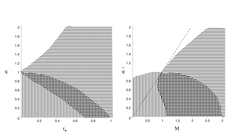
FIG. 1.: In Figure 1a stability domains are plotted as ${q}$ vs. ${{r_{+}}}$ for the grand-canonical ensemble of $D=5$ R-charged black holes with one charge turned on. In Figure 1b the same stability plots are exhibited, but now as ${\tilde{q}}$ (the physical charge) vs. $M$ (the ADM mass). Only the region satisfying the BPS bound, $M\geq{\tilde{q}}$, corresponds to physical black hole solutions. The vertically shaded areas correspond to the regions where the $AdS_{5}$ is the preferred solution and the horizontally shaded area correspond to the regions where the black hole solutions are local minimum of the Gibbs action. The checkered area is the domain of common overlap: there black holes still correspond to the local maxima of the entropy (local minima of the Euclidean action); however, anti-de Sitter space is preferred globally. In the unshaded area, neither the black hole solution nor pure anti-de Sitter space are global minima of the action.

C Canonical Ensemble

We now repeat the stability analysis for the canonical ensemble; along with the fixed inverse temperature $\beta$ , one now fixes the physical charges ${\tilde{q}}_{i}$, i.e., the field strengths $F_{\mu,\nu}^{i}$ (and not the electric potentials $\phi_{i}$) are fixed. Following a procedure analogous to the one spelled out for the grand-canonical ensemble in Subsection III B, but now with the new boundary conditions, one obtains the following form of the Helmholtz Euclidean action:

$$I_{H}=\beta M-S\ ,$$ (26)

where $M$ and $S$ are the mass and the entropy of the system and $\beta$ is the inverse temperature. Extremizing the above action with respect to $S$, or equivalently, with respect to $r_{+}$ (while keeping the physical charges ${\tilde{q}}_{i}$ fixed) determines the correct inverse temperature $\beta$ of the black hole solution (10).

To locate the Hawking-Page transition, we write the Helmholtz action (26) for the black hole solution described in Section II as a function of $q_{i}$ and $r_{+}$:

$$I_{H}^{BH}={\beta\over{2r_{+}^{2}}}\left[r_{+}^{4}(1-r_{+}^{2})+r_{+}^{2}\sum_{i=1}^{3}q_{i}(2+r_{+}^{2})+3r_{+}^{2}\sum_{i<j}^{3}q_{i}q_{j}+5\prod_{i=1}^{3}q_{i}\right]\ ,$$ (27)

where $\beta$ is defined in (10). The phase transition between the black hole solution and the pure $AdS_{5}$ solution is determined by the zero of $I_{H}^{BH}$ (27):

$$q_{0}(r_{+})={{r_{+}^{2}(r_{+}^{2}-1)}\over{2+r_{+}^{2}}}\ .$$ (28)

In the domain $q>q_{0}(r_{+})$ the black hole solution has $I_{H}<0$ and thus it is the dynamically preferred solution. (For $q_{0}=0$ the critical point is again $r_{+}=1$ [${\tilde{q}}=0$, $M=3$].)

To evaluate local thermodynamic stability, we use the method outlined in Subsection III A around equation (19). In the case of a single non-zero charge, say $q_{1}=q\neq 0$, the local stability constraint leads to:

$$2r_{+}^{4}+r_{+}^{2}(5q+1)-q^{2}+6q-1\geq 0\ .$$ (29)

This case is simple enough that one can easily verify (29) by explicitly computing $\left({\partial^{2}S\over\partial M^{2}}\right)_{q}$. The zeroes of the left hand side of (29) form two critical lines:

$$q_{\pm}(r_{+})=1+\textstyle{5\over 2}r_{+}^{2}\pm\textstyle{1\over 2}\sqrt{32+64r_{+}^{2}+33r_{+}^{4}}\ ,$$ (30)

and the stable region corresponds to the domain $q_{-}(r_{+})\leq q\leq q_{+}(r_{+})$. Again, $q_{-}=0$ corresponds to the critical point: $r_{+}\leq{1\over\sqrt{2}}$ [${\tilde{q}}=0$, $M={9\over 8}$] [10]. On the other hand now the stable domain with $r_{+}=0$ corresponds to the range of charges: $3-2\sqrt{2}\leq q\leq 3+2\sqrt{2}$. [Equivalently, this is the region with $M={\tilde{q}}$ (BPS-limit) and $3-2\sqrt{2}<{\tilde{q}}=q<3+2\sqrt{2}$.] Black holes in the region $q<q_{-}(r_{+})$ and $q>q_{+}(r_{+})$ are not thermodynamically stable.

In Figure 2a we show the stability regions in a plot of $q$ vs. $r_{+}$. In Figure 2b we exhibit the same stability regions plotting ${\tilde{q}}$ vs. $M$. The vertically shaded areas correspond to the regions where the $AdS_{5}$ is the preferred solution and the horizontally to the regions where the black hole solution is the local minimum of the Helmholtz action.

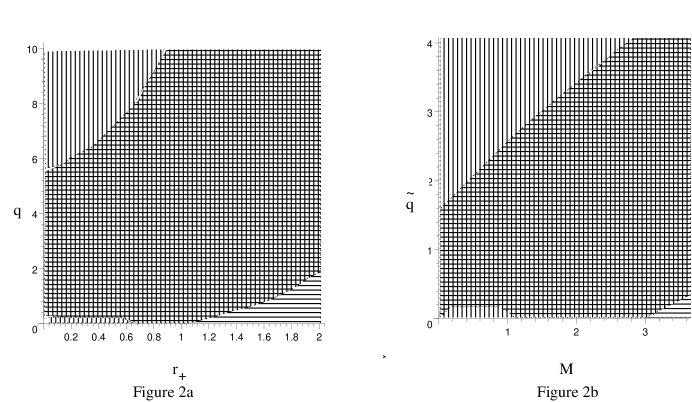
FIG. 2.: In Figure 2a we plot the stability domains as $q$ vs. $r_{+}$ for the canonical ensemble of $D=5$ R-charged black holes with one non-zero charge. In Figure 2b the same stability plots are exhibited, but now plotting ${{\tilde{q}}}$ vs. ${M}$. The vertically shaded areas are the regions where anti-de Sitter space is the preferred solution. The horizontally shaded areas are the regions where the black hole solution is a local minimum of the Helmholtz action. The checkered area is the domain of common overlap: meta-stable black holes in the intepretation of section III B.

Note three salient differences between the results for the canonical and grand-canonical ensembles. First, as expected from the general considerations of Subsection III A, the region of local stability for the canonical ensemble is larger than for the grand-canonical ensemble. Second, the region favored by the pure $AdS_{5}$ is significantly increased for the canonical ensemble, and it encompasses the whole region with $r_{+}<1$ and non-zero $q_{i}$’s. Third, and most interesting, the pure $AdS_{5}$ space-time is dynamically favored in the whole domain of the black hole parameters for which the black holes are locally unstable.

IV Spinning D3-branes as R-charged black holes

In this Section we establish the precise connection between the near-extreme spinning D3-branes solution and the solutions of $N=8$, $D=5$ gauged supergravity found in [10] and discussed in Section II. In this Section we restore all factors of $L$ explicitly, but still set $G_{5}={\pi\over 4}$.

A Equivalence of $k=0$ R-charged black holes and near-extreme spinning D3-branes

Angular momenta in planes perpendicular to the world-volume of D3-branes (which we refer to as spins to distinguish them from angular momenta in other planes) are realized in the world-volume theory as charges under the global $SO(6)$ R-symmetry group. In the reduction of type IIB supergravity on $S^{5}$, the $SO(6)$ isometry becomes the non-abelian gauge symmetry of the resulting ${\cal N}=8$ gauged supergravity in five dimensions, and the spins become $SO(6)$ gauge charges. In the AdS/CFT correspondence, the $SO(6)$ supergravity gauge fields in the bulk of $AdS_{5}$ couple to the gauge theory R-currents on the boundary. It is well-known that the near-horizon geometry of near-extreme D3-branes without spin reduces to a Schwarzschild black hole in $AdS_{5}$. The purpose of this section is to show how spin on the D3-branes reduces to charge on the black holes. By explicitly performing the Kaluza-Klein reduction on $S^{5}$, we will obtain the precise relationship between the parameters of the R-charged black holes and those of the spinning D3-branes. For the sake of simplicity only one angular momentum, so that the black hole will have $q_{1}=q\neq 0$ but $q_{2}=q_{3}=0$. One can verify that the computation extends to the case of all three angular momenta non-zero.

The near-horizon form of the ten-dimensional D3-brane solution with a single angular momentum is [17, 18]

$${ds_{10}^{2}}$$

(31)

The basic Kaluza-Klein ansatz is [19]

$$\hat{g}_{MN}=\pmatrix{e^{-{4\over 3}D}g_{\mu\nu}+A_{\mu}{}^{\gamma}A_{\mu\gamma}&A_{\mu\beta}\cr A_{\nu\alpha}&G_{\alpha\beta}}\ ,$$ (32)

where indices $\alpha,\beta,\gamma$ run over the compact internal manifold $K$, and $\mu,\nu$ run over the non-compact spacetime $M$. The metric on $K$ can vary with the position on $M$, and the equation

$$\mathop{\rm vol}\nolimits_{K}=e^{2D}\mathop{\rm vol}\nolimits_{K,\infty}$$ (33)

defines the “dilaton” field $D$ (not to be confused with the ten-dimensional dilaton $\phi$) in terms of how the volume form on $K$ compares to its limit at spatial infinity. The power of $e^{D}$ in (32) is chosen to put the metric $g_{\mu\nu}$ in Einstein frame. For the solution (31) we have

$${ds_{K}^{2}}$$

(34)

The only non-zero component of $A_{\mu}{}^{\gamma}$ is

$$A_{t}{}^{\phi}=-{\ell r_{0}^{2}\over L^{2}r^{2}\tilde{\Delta}}\ .$$ (35)

Finally, the five-dimensional metric $g_{\mu\nu}$ is just the solution (4) with $k=0$, $\mu=r_{0}^{4}/L^{2}$, $q_{1}=\ell^{2}$, and $q_{2}=q_{3}=0$. Note that although $D$ and $ds_{K}^{2}$ vary over both $M$ and $K$, the five-dimensional metric $ds_{M}^{2}$ and the five-dimensional gauge potential $A_{t}{}^{\phi}$ are independent of the internal coordinates. The dependence of $D$ on $K$ indicates that the compactification is a warped product.

There is a slight subtlety in comparing the gauge fields in (42) of [10] with (35): superficially in [10] the field strength seems to vanish because of an explicit prefactor of $\sqrt{k}$. At this point it is useful to recall the approach of [3] where the $k=0$ solution is recovered by focusing in on a small, nearly flat part of the $S^{3}$ in the $k=1$ solution. This amounts to taking the limit $k\to 0+$. In this limit, $q=\ell^{2}$ and $\mu=r_{0}^{4}/L^{2}$ are held fixed. From equation (43) of [10] one obtains $\sinh^{2}\beta=k\ell^{2}L^{2}/r_{0}^{4}$. The factor of $k$ in this relation conspires to cancel the one explicitly shown in (42) of [10], and the end result for the gauge field $A^{1}$ pertaining to the charge $q_{1}$ is

$$A^{1}_{t}={L\over 2}A_{t}{}^{\phi}\ .$$ (36)

The factor of ${L\over 2}$ comes from a different choice of normalization of $A_{\mu}$ in [10]. For us the gauge kinetic term picks up a factor of $L$ from $\sqrt{G}G^{-1}G^{-1}$.

There is some debate over the status of five-dimensional ${\cal N}=8$ gauged supergravity as a truncation of the Kaluza-Klein reduction of type IIB supergravity/string theory. In particular, is it true that solutions of the former can always be promoted to solutions of the latter? This seems guaranteed for supersymmetric solutions from closure properties of the supersymmetry algebra, but for non-supersymmetric solutions one is making a nontrivial statement regarding the equations of motion. Modulo the small technical issue of compactifying ${\bf R}^{3}$ to $S^{3}$, non-extreme R-charged black holes provide an example of a non-supersymmetric solution of gauged supergravity which can indeed be promoted to a solution in ten dimensions: namely the spinning D3-brane solution. The key point is that the gauge potential $A_{t}{}^{\phi}$ and the metric $g_{\mu\nu}$ resulting from the Kaluza-Klein compactification of the spinning D3-brane solution are independent of the $S^{5}$ coordinates.

B Thermodynamic equivalence of large R-charged black holes and spinning D3-branes

Another way to view the $k\to 0^{+}$ limit is that black hole solutions with $k=0$ can be recovered from large black hole solutions with $k=1$ by restricting attention to a angular region of the $S^{3}$ in the $k=1$ region where the curvature can be neglected. This was explained precisely for Schwarzschild black holes in [3], and the same story goes through with charged black holes. New physics shows up in the $k=1$ solutions (for instance, the confinement-deconfinement transition) because of the finite-size effects of the $S^{3}$. When we take $k\to 0^{+}$, we are making the volume of the $S^{3}$ very large compared to the cube of the inverse temperature. Neglecting all finite size effects should lead us back to the thermodynamics of spinning D3-branes whose world-volume is flat and infinite. The purpose of this Subsection is to show this explicitly and to establish the precise connection between the respective physical parameters.

Large R-charged black holes are the ones with $r_{+}\gg L$ and $q_{i}\gg L^{2}$. In this limit, the expressions for the ADM mass $M$ (8) and the physical charges ${\tilde{q}}_{i}$ (11) reduce to the following form:

$$M\sim\textstyle{3\over 2}\mu,\ \ {\tilde{q}}_{i}^{2}\sim q_{i}\mu\ ,\ \ (i=1,2,3)\ ,$$ (37)

where $\mu$ is related to $r_{+}$ and $q_{i}$’s by $f(r_{+})=0$ (see eq.(5)). In the large charge limit this equation implies:

$${1\over L^{2}}\prod_{i=1}^{3}(r_{+}^{2}+q_{i})-\mu r_{+}^{2}\sim 0\ .$$ (38)

To obtain (38), one can start with $f(r_{+})r_{+}^{4}=0$ and drop the term $kr_{+}^{4}$. This makes sense in view of the equivalence of $k\to 0^{+}$ and large $k=1$ black holes.

By introducing new variables

$$y_{H}\equiv\alpha^{-1}\sqrt{\mu}r_{+},\ \ y_{i}\equiv\alpha^{-1}{{\tilde{q}}_{i}}\ ,(i=1,2,3)\ ,$$ (39)

where $\alpha=(\mu^{3}L^{2})^{1/4}$, one can rewrite (38) in the following form:

$$\prod_{i=1}^{3}(y_{H}^{2}+y_{i}^{2})-y_{H}^{2}=0\ .$$ (40)

This is precisely the “horizon” equation for spinning D3-branes displayed in Section II of Ref. [6].

One can introduce the energy density $e$, entropy density $s$ and the charge density $j_{i}$ in the following way:

$$e \equiv {M\over{N^{2}V}}\ ,$$ (41)

$$j_{i} \equiv {{{\tilde{q}}_{i}}\over{N^{2}V}}={s\over{2\pi}}{y_{i}\over y_{H}}\ ,$$ (42)

$$s \equiv {S\over{N^{2}V}}=2\pi\gamma e^{3/4}y_{H}\ ,$$ (43)

where

$$V=2\pi^{2}L^{3},\ \ N^{2}=2L^{3},\ \ \gamma={2\over{27\pi^{2}}}\ .$$ (44)

The thermodynamic variables introduced in (43), together with the definition of the volume $V$ and the flux $N$ (44) in terms of $L$ (and $G_{5}$ if we hadn’t set it equal to $\pi/4$) and also the relationship between $y_{H}$ and $y_{i}$ (39), provides a precise translation of the thermodynamic variables of large black holes into those of spinning D3-branes. It may seem strange to assign a definite volume to the $S^{3}$ on the boundary of $AdS_{5}$. However, as commented on in [20] and [21], a choice of radial coordinate is equivalent to choosing a definite metric among those with a specified conformal structure. Our choice of radial coordinate was fixed in (4).

Even in view of the above translation of variables, the equivalence between the local thermodynamic stability constraints for spinning branes and R-charged black holes is slightly non-trivial: equations (37) and (43) define a non-linear relation between $e$ and $j_{i}$ for the spinning brane and $M$ and $\tilde{q}_{i}$ for the R-charged black hole. To see that the stability constraints must turn out the same, think of this relation as a reparametrization of phase space, similar to the convenient $(r_{+},q_{i})$ parametrization we used in earlier sections. The argument in Section III A should guarantee that the stability region does not depend on the reparametrization. In the case of one non-zero charge, the stability constraints for R-charged black holes for the grand-canonical ensemble (23) and canonical ensemble (29) reduce to the following respective forms in the $r_{+}/L\to\infty$, $q/L^{2}\to\infty$ limit:

$$2 r_{+}^{2}-q={\mu\over\alpha^{2}}y_{H}^{2}(2-x^{2})\geq 0\qquad\hbox{grand-canonical}$$ (45)

$$2 r_{+}^{4}+5r_{+}^{2}q-q^{2}={\mu\over\alpha^{2}}y_{H}^{2}(2+5x^{2}-x^{4})\geq 0\qquad\hbox{canonical.}$$ (46)

Here $x\equiv{y\over y_{H}}$. These stability constraints are in precise agreement [5, 7] with those of near-extreme spinning D3-branes with only one angular momentum turned on.

V Phases of R-charged black holes in $D=4$

So far we have focused our attention on black holes in $AdS_{5}$ because they are dual to thermal states of ${\cal N}=4$ supersymmetric gauge theory in 3+1 dimensions. Our analysis is extended in this section and the next to black holes in maximally supersymmetric gauged supergravity in $D=4$ and $D=7$. In Section VII we outline their relationship with spinning M2- and M5-branes.

Black holes in $D=4$ $N=8$ gauged supergravity have been studied in Ref. [11]. Their Einstein frame metric is of the following form [11, 22]:

$$ds^{2}=-{(\prod_{i=1}^{4}H_{i})^{-1/2}}fdt^{2}+(\prod_{i=1}^{4}H_{i})^{1/2}\bigg{(}f^{-1}{dr^{2}}+r^{2}d\Omega_{2,k}\bigg{)}\ ,$$ (47)

where

$$f=k-{\mu\over r}+g^{2}r^{2}\prod_{i=1}^{4}H_{i}\ ,\ \ H_{i}=1+{{q_{i}}\over r},\ (i=1,\cdots 4)\ .$$ (48)

Here we have chosen $G_{4}={1\over 4}$. (Again we shall concentrate on black hole solutions with $k=1$.) With this choice of $G_{4}$, $q_{i}$’s and the physical charges ${\tilde{q}}_{i}$’s are defined in (7) and the ADM mass is of the following form:

$$M=2\mu+\sum_{i=1}^{4}q_{i}=2(r_{+}+r_{+}^{3}g^{2}\prod_{i=1}^{4}H_{i})+\sum_{i=1}^{4}q_{i}\ ,$$ (49)

where in the second equality the radial coordinate at the outer horizon $r_{+}$ is defined as the largest non-negative zero of $f(r)$ (48).

Again the parameterization of the thermodynamic quantities in terms of $q_{i}$ and $r_{+}$ (instead of ${\tilde{q}}_{i}$ and $M$) is most suitable:

$$S={A\over{4G_{4}}}=4\pi\sqrt{\prod_{i=1}^{4}(r_{+}+q_{i})}\ ,$$ (50)

$$\beta={1\over T_{H}}={{4\pi r_{+}\sqrt{\prod_{i=1}^{4}(r_{+}+q_{i})}}\over{3r_{+}^{4}+2r_{+}^{3}\sum_{i=1}^{4}q_{i}+r_{+}^{2}(\sum_{i<j}^{4}q_{i}q_{j}+1)-\prod_{i=1}^{4}q_{i}}}.$$ (51)

The physical charges are then determined in terms of $q_{i}$ and $r_{+}$ in the following way:

$${\tilde{q}}_{i}^{2}=q_{i}(r_{+}+q_{i})\left[1+{1\over r_{+}}\prod_{j\neq i}(r_{+}+q_{j})\right]\ ,$$ (52)

and the electric potentials at the outer horizon take the following form:

$$\phi_{i}=A^{i}_{t}(r_{+})={{\tilde{q}_{i}}\over{r_{+}+q_{i}}}\ ,\ (i=1,\cdots,4)\ .$$ (53)

In the following, along with $G_{4}={1\over 4}$ we shall also take $L\equiv{1\over g}=1$. (Note $L$ is related to the asymptotic cosmological constant $\Lambda=-{3\over L^{2}}$.) However, $L$ can be restored by replacing $r_{+}$ by ${r_{+}\over L}$ and $q_{i}$ by ${q_{i}\over L}$.

A Grand-Canonical Ensemble and Stability Constraints

The Gibbs Euclidean action is of the form:

$$I_{G}=\beta(M-\sum_{i=1}^{4}{\tilde{q}}_{i}\phi_{i})-S\ ,$$ (54)

where $M$ is the mass, ${\tilde{q}}_{i}$ is the physical charge and $S={A\over{4G_{4}}}$ is the entropy. The extrema of this action correspond to the black hole solutions for which the inverse Hawking temperature and the electric potentials at the outer horizon are given in (51) and (53), respectively.

The critical hypersurfaces of thermodynamic stability can again be determined by evaluating the zeroes of the determinant of the Hessian of second derivatives of (54) with respect to $r_{+}$ and $q_{i}$.

The phase transition between the black hole solutions and pure $AdS_{4}$ occurs when (54) for the black hole solution ceases to be negative. When expressed explicitly in terms of $q_{i}$ and $r_{+}$, (54) takes the following suggestive form:

$$I_{G}^{BH}={\beta\over{r_{+}}}\left[r_{+}^{2}-\prod_{i=1}^{4}(r_{+}+q_{i})\right]\ ,$$ (55)

where $\beta$ is determined by (51).

For one non-zero charge only, say $q_{1}=q\neq 0$, the the region of local thermodynamic stability is specified by

$$3r_{+}^{4}+qr_{+}^{3}-2q^{2}r_{+}^{2}+2r_{+}^{2}+3qr_{+}-1\geq 0\ .$$ (56)

The zeroes of the above expression correspond to two critical lines:

$$q_{\pm}(r_{+})={3\over{4r_{+}}}+{r_{+}\over{4}}\pm{1\over 4}\sqrt{{1\over r_{+}^{2}}+22+25r_{+}^{2}}\ ,$$ (57)

with the stable domain satisfying $q_{-}(r_{+})<q<q_{+}(r_{+})$. $q_{-}=0$ has a critical point at $r_{+}={1\over\sqrt{3}}$ [8]. Note also that as $r_{+}\to 0$ the local stability region is pushed to large $q$: $q_{\pm}\to\infty$ as $r_{+}\to 0$.

The phase transition between the black hole solution and the pure $AdS_{4}$ solution is now determined by:

$$q_{0}(r_{+})={1\over r_{+}}-r_{+}\ .$$ (58)

For $q>q_{0}(r_{+})$ the black holes are dynamically preferred over $AdS_{4}$. As $r_{+}\to 0$, the critical line is pushed to $q_{0}\to\infty$. $q_{0}=0$ has the Hawking-Page transition at $r_{+}=1$ [8].

For $q>q_{+}(r_{+})>q_{0}(r_{+})$ black holes unstable, but at the same time the pure $AdS_{4}$ space-time is not dynamically preferred either. The region $q_{-}(r_{+})<q<q_{0}(r_{+})$ corresponds to the domain where $AdS_{4}$ is entropically favored, but the black hole solution still corresponds to a local minimum of the Gibbs action (54).

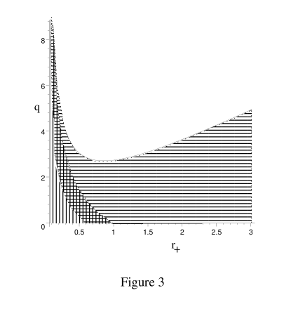
FIG. 3.: The stability domains as ${q}$ vs. ${{r_{+}}}$ for the grand-canonical ensemble of $D=4$ R-charged black holes with one non-zero charge are given. The vertically shaded areas correspond to the regions where the $AdS_{4}$ is the preferred solution and the horizontally shaded area correspond to the regions where the black hole solutions are local minimum of the Gibbs action. The checkered area is the domain of common overlap. The unshaded area corresponds to black holes that are unstable but nevertheless favored over pure anti-de Sitter space. Explicit powers of $L$ can be restored by replacing $r_{+}$ with ${r_{+}\over L}$ and $q$ with ${{q}\over L}$.

In Figure 3 we plot all these stability regions for $q$ vs. $r_{+}$. The vertically shaded area corresponds to the regions where the $AdS_{4}$ is the preferred solution and the horizontally shaded area corresponds to the region where the black hole solution is the local minimum of the Gibbs action.

B Canonical Ensemble and Stability Constraints

Repeating the same analysis now for the canonical ensemble yields the Helmholtz action (26) which for $D=4$ black holes takes the following form:

$$I_{H}^{BH}={\beta\over{r_{+}}}\left[-r_{+}^{4}+r_{+}^{2}(1+\sum_{i<j}^{4}q_{i}q_{j})+r_{+}(\sum_{i=1}^{4}q_{i}+2\sum_{i<j<k}^{4}q_{i}q_{j}q_{k})+3\prod_{i=1}^{4}q_{i}\right]\ ,$$ (59)

where $\beta$ is defined in (51). $I_{H}^{BH}$ (59) differs significantly from $I_{G}^{BG}$ (55).

In the case of a single non-zero charge the local stability constraint leads to:

$$3r_{+}^{5}+6qr_{+}^{4}+2r_{+}^{3}+7qr_{+}^{2}+2q^{2}r_{+}-r_{+}-q\geq 0\ .$$ (60)

The critical line now has only one branch:

$$q_{-}(r_{+})={1\over{4r_{+}}}\left(-6r_{+}^{4}-7r_{+}^{2}+1+\sqrt{36r_{+}^{8}+60r_{+}^{6}+21r_{+}^{4}-6r_{+}^{2}+1}\right)\ ,$$ (61)

with the region $q\geq q_{-}(r_{+})$ stable.

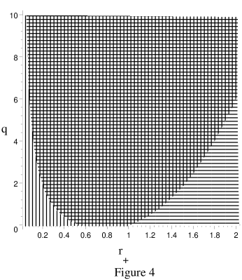
FIG. 4.: The stability domains are plotted for ${q}$ vs. ${{r_{+}}}$ for the canonical ensemble of $D=4$ R-charged black holes with one non-zero charge. The vertically shaded areas indicates the regions where $AdS_{4}$ is the preferred solution, and the horizontally shaded area shows the regions where the black hole solutions are local minima of the Helmholtz action. The checkered area is the domain of common overlap. Explicit powers of $L$ can be restored by replacing $r_{+}$ with ${r_{+}\over L}$, and $q$ with ${{q}\over L}$.

The phase transition between the black hole solution and the pure $AdS_{4}$ solution now takes place along the line

$$q_{0}(r_{+})=r_{+}^{3}-r_{+}\ .$$ (62)

For $q>q_{0}(r_{+})$ the black hole solution is the dynamically preferred solution. Pure $AdS_{4}$ is dynamically favored in the whole domain where the black hole is thermodynamically unstable.

In Figure 4 we plot the stability regions for $q$ vs. $r_{+}$. The vertically shaded area corresponds to the regions where $AdS_{4}$ is the preferred solution, and the horizontally shaded area corresponds to the region where the black hole solution is a local minimum of the Helmholtz action.

VI Phases of R-charged black holes in $D=7$

We quote the black hole solution of $N=4$ gauged supergravity in $D=7$ (While the solution has not been derived from the actual $D=7$ Lagrangian the structure of this solution is in close analogy with the structure of the R-charged solution in $D=4$ and $D=5$.):

$$ds^{2}=-{(H_{1}H_{2})^{-{4/5}}}fdt^{2}+(H_{1}H_{2})^{1/5}\bigg{(}f^{-1}{dr^{2}}+r^{2}d\Omega_{5,k}\bigg{)}\ ,$$ (63)

where

$$f=k-{\mu\over r^{4}}+g^{2}r^{2}H_{1}H_{2}\ ,\ \ H_{i}=1+{{q_{i}}\over r^{4}},\ (i=1,2)\ .$$ (64)

We have chosen $G_{7}={\pi^{2}\over 4}$. We are most interested in the case $k=1$. The $q_{i}$ and ${\tilde{q}}_{i}$ are again related by (7) and the mass is specified as:

$$M={\textstyle{5\over 4}}\mu+q_{1}+q_{2}=\textstyle{5\over 4}(r_{+}^{4}+r_{+}^{6}g^{2}H_{1}H_{2})+q_{1}+q_{2}\ ,$$ (65)

where again in the second equality the radial coordinate at the outer horizon $r_{+}$ is defined as the largest non-negative zero of $f(r)$ (64).

The parameterization of the thermodynamic quantities in terms of of $q_{i}$ and $r_{+}$ yields the following expressions:

$$S={A\over{4G_{7}}}=\pi r_{+}\sqrt{(r_{+}^{4}+q_{1})(r_{+}^{4}+q_{2})}\ ,$$ (66)

$$\beta={1\over T_{H}}={{\pi r_{+}^{3}\sqrt{(r_{+}^{4}+q_{1})(r_{+}^{4}+q_{2})}}\over{3r_{+}^{8}+2r_{+}^{6}+r_{+}^{4}(q_{1}+q_{2})-q_{1}q_{2}}}.$$ (67)

The physical charges are then determined in terms of $q_{i}$ and $r_{+}$ in the following way:

$${\tilde{q}}_{i}^{2}=q_{i}(r_{+}^{4}+q_{i})\left[1+{1\over r_{+}^{2}}(r_{+}^{4}+q_{j})\right]\ ,\ (j\neq i)\ ,$$ (68)

and the electric potentials at the outer horizon take the following form:

$$\phi_{i}=A^{i}_{t}(r_{+})={{\tilde{q}_{i}}\over{r_{+}^{4}+q_{i}}}\ ,\ (i=1,2)\ .$$ (69)

In the following we set $L\equiv{1\over g}=1$. $L$, which is related to the asymptotic cosmological constant $\Lambda=-{{15}\over L^{2}}$, can be restored by replacing $r_{+}$ by ${r_{+}\over L}$ and $q_{i}$ by ${q_{i}\over L^{4}}$.

A Grand-Canonical Ensemble and Stability Constraints

$I_{G}$ for the black hole solution, when expressed explicitly in terms of $q_{i}$ and $r_{+}$, takes the form:

$$I_{G}^{BH}={\beta\over{2r_{+}^{2}}}\left[r_{+}^{6}-(r_{+}^{4}+q_{1})(r_{+}^{4}+q_{2})\right]\ ,$$ (70)

where $\beta$ is determined by (67).

For one non-zero charge only, the thermodynamic stability constraint takes the following form:

$$3r_{+}^{8}+r_{+}^{6}+2qr_{+}^{4}-2r_{+}^{4}+3qr_{+}^{2}-q^{2}\geq 0\ .$$ (71)

The critical line has two branches:

$$q_{\pm}(r_{+})=r_{+}^{2}\left(r_{+}^{2}+\textstyle{3\over 2}+\textstyle{1\over 2}\sqrt{16r_{+}^{4}+16r_{+}^{2}+1}\right)\ ,$$ (72)

and the region of local stability is $q_{-}(r_{+})<q<q_{+}(r_{+})$. $q=0$ has the critical point at $r_{+}=\sqrt{2\over 3}$. Note also that as $r_{+}\to 0$ the critical line is pushed to $q_{\pm}\to 0$.

The phase transition between the black hole solution and the pure $AdS_{7}$ takes place at $q_{0}(r_{+})=0$, where

$$q_{0}(r_{+})=r_{+}^{2}-r_{+}^{4}\ .$$ (73)

For $q>q_{0}(r_{+})$ the black hole is the dynamically preferred solution. As $r_{+}\to 0$ the critical line is pushed to $q_{0}\to 0$. When $q_{0}=0$, the Hawking-Page transition is at $r_{+}=1$. In the region $q>q_{+}(r_{+})>q_{0}(r_{+})$, the black hole solutions are unstable, but $AdS_{7}$ is not dynamically preferred either.

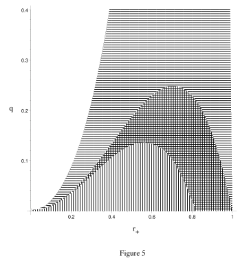
FIG. 5.: The stability domains as ${q}$ vs. ${{r_{+}}}$ for the grand-canonical ensemble of $D=7$ R-charged black holes with one non-zero charge. The vertically shaded areas correspond to the regions where the $AdS_{7}$ is the preferred solution and the horizontally shaded area correspond to the regions where the black hole solutions are local minimum of the Gibbs action. The checkered area is the domain of common overlap. The unshaded area is where neither black holes nor anti-de Sitter space are stable. Powers of $L$ can be restored by replacing $r_{+}$ with ${r_{+}\over L}$ and $q$ with ${{q}\over L^{4}}$.

In Figure 5 the stability regions are shown in a plot of $q$ vs. $r_{+}$.

B Canonical Ensemble and Stability Constraints

Repeating the same analysis for the canonical ensemble yields the Helmholtz action (26) which for the black hole solution takes the following form:

$$I_{H}^{BH}={\beta\over{2r_{+}^{2}}}\left[-r_{+}^{8}+r_{+}^{6}+(3r_{+}^{4}+4r_{+}^{2})(q_{1}+q_{2})+7q_{1}q_{2}\right]\ ,$$ (74)

with $\beta$ defined in (67).

In the case on single non-zero charge, the local stability constraint leads to:

$$3r_{+}^{10}+r_{+}^{8}-2r_{+}^{6}+12qr_{+}^{6}+17qr_{+}^{4}+4qr_{+}^{2}-3r_{+}^{2}q^{2}-2q^{2}\geq 0\ .$$ (75)

The critical line has two branches:

$$q_{\pm}(r_{+})={{r_{+}^{2}}\over{2(2+3r_{+}^{2})}}\left(17r_{+}^{2}+4+12r_{+}^{4}+\sqrt{180r_{+}^{8}+444r_{+}^{6}+369r_{+}^{4}+120r_{+}^{2}+16}\right)\ ,$$ (76)

with $q_{-}(r_{+})\leq q\leq q_{+}(r_{+})$ corresponding to the stable region. Note that as $r_{+}\to 0$, the critical lines are pushed to $q_{\pm}\to 0$.

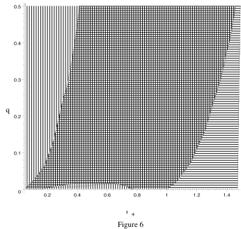
FIG. 6.: The stability domains ${q}$ vs. ${{r_{+}}}$ for the canonical ensemble of $D=7$ R-charged black holes with one non-zero charge are given. The vertically shaded areas correspond to the regions where the $AdS_{7}$ is the preferred solution and the horizontally shaded area correspond to the regions where the black hole solutions are local minimum of the Helmholtz action. The checkered area is the domain of common overlap. The units of $L=1$ can be restored by replacing $r_{+}$ with ${r_{+}\over L}$, and $q$ with ${{q}\over L^{4}}$.

The Hawking-Page transition between the black hole solution and the pure $AdS_{7}$ solution is now determined by $q_{0}(r_{+})=0$, where

$$q_{0}(r_{+})={{r_{+}^{6}-r_{+}^{4}}\over{4r_{+}^{2}+3}}\ .$$ (77)

For $q>q_{0}(r_{+})$ the black hole solution is the dynamically preferred solution. As $r_{+}\to 0$, $q_{0}\to 0$. In Figure 6 these stability domains are shown in a plot of $q$ vs. $r_{+}$.

VII R-charged black holes in $D=5$ ($D=7$) and spinning M2 (M5)-branes

The Kaluza-Klein reduction described in Section IV of spinning D3-branes to R-charged black holes in $AdS_{5}$ can be repeated for spinning M2- and M5-branes [23], and it leads to R-charged black holes in $AdS_{4}$ and $AdS_{7}$. As in Subsection IV B, one can also obtain the precise translation from the mass $M$, charges $\tilde{q}_{i}$, and the entropy of large R-charged black holes in $AdS_{4}$ [$AdS_{7}$], to the energy $E$ above extremality, the angular momenta $J_{i}$, and the entropy $S$ of near-extreme spinning M2-branes [M5-branes].

As a consequence of this equivalence, the thermodynamic stability constraints derived for the general spinning M2-branes [and M5-branes] should coincide with those of large R-charged black holes in $D=4$ [and $D=7$], respectively. For the case of only one non-zero charge the grand-canonical ensemble (56) [(71)] and canonical ensemble (56) [and (71)] stability constraints reduce in the case of large R-charged black holes ($r_{+}\gg 1$ and $q\gg 1$) to the following stability constraints:

$$3r_{+}-2q\geq 0\ ,\ \ D =4,\ \hbox{grand-canonical}\ ,$$ (78)

$$r_{+}+2q\geq 0\ ,\ \ D =4,\ \hbox{canonical}\ ,$$ (79)

$$[\ \ 3r_{+}^{4}-q\geq 0\ ,\ \ D =7,\ \hbox{grand-canonical}\ ,$$ (80)

$$r_{+}^{8}+4r_{+}^{4}q-q^{2}\geq 0\ ,\ \ D =7,\ \hbox{canonical}\ \ ]$$ (81)

which agree precisely with the respective stability constraints [7, 6] for spinning M2-branes [and M5-branes] with only one angular momentum turned on.

Finally, we would like to note a feature of the asymptotics of the stability conditions for small and large $q$ which may be only numerological coincidence, but seems to us intriguing. There is an exponent $\alpha_{p}$ which characterizes the scaling of the entropy $S$ of near-extreme non-dilatonic $p$-branes with the number $N$ of branes: $S\sim N^{\alpha_{p}}$. For $p=3$ (the D3-brane), $\alpha_{3}=2$, which is interpreted as evidence that there are indeed on the order of $N^{2}$ degrees of freedom on the world-volume, as expected in a conformally invariant gauge theory with gauge group $SU(N)$. For $p=2$ (the M2-brane), $\alpha_{2}=3/2$. For $p=5$ (the M5-brane), $\alpha_{5}=3$. Cross-sections of minimal scalars falling into any of these branes have the same $N^{\alpha_{p}}$ scaling [24, 25]. We note for the record that $\alpha_{p}={d-3\over d-5}$ where $d$ is one plus the number of spatial dimensions perpendicular to the brane world-volume.

In the grand-canonical ensemble, the ratio of charge to mass where stability is lost for large R-charged black holes in $D=4$ [$D=7$] is most efficiently expressed as $\sqrt{r_{+}\over q}=\sqrt{2\over 3}=(\alpha_{2})^{-1/2}$ [$\sqrt{r_{+}^{4}\over q}={1\over\sqrt{3}}=(\alpha_{5})^{-1/2}$]. On the other hand, in the $q\to 0$ limit, the critical mass where stability is lost can be determined from $r_{+}={1\over\sqrt{3}}$ [$r_{+}=\sqrt{2\over 3}$] in $D=4$ [$D=7$]. Thus the $D=4$ and $D=7$ results are in a peculiar numerological sense dual to one another. For the case of R-charged black holes in $D=5$, the large black hole stability constraint and that of $q=0$ are self-dual: $\sqrt{r_{+}^{2}\over q}={1\over\sqrt{2}}=(\alpha_{3})^{-1/2}$ for large $q$, and $r_{+}={1\over\sqrt{2}}$ for small $q$.

VIII Conclusions

One of the motivations for this work was the question, “What happens in a quantum theory of gravity when a black hole becomes thermodynamically unstable?” String theory in principle provides us with a venue to address this question. In general, however, the black holes of which one has a good string theory description are thermodynamically stable. A possible exception, first noted in [5], is D3-branes with spin, by which we mean angular momentum in a plane transverse to the world-volume. These objects, which we have shown to reduce to charged black holes in $AdS_{5}$, can become unstable due to excessively large spin—or, in the five-dimensional picture, excessive charge.

We had initially hoped to show that the charge-driven instability of black holes in $AdS_{5}$ could be understood in terms of the Hawking-Page transition: that is, for the black holes which were thermodynamically unstable, there would be a transition to a gas of charged particles in pure anti-de Sitter space. To a first approximation, this transition occurs when the Euclidean action of the black hole solution rises above the Euclidean action for pure anti-de Sitter space subjected to the same boundary conditions at spatial infinity.

This hope was only partly substantiated, and an intricate phase diagram realized, through analytic treatments of the local thermodynamic stability conditions and of the criterion for the Hawking-Page transition. Holding temperature and electric potential fixed, we found in particular that there is a region of phase space where the black hole solution is locally unstable (that is, it is only a saddle point and not a local minimum of the Euclidean action), but where pure anti-de Sitter space has a still higher action! In this region, neither the black hole solution nor the gas of particles in anti-de Sitter space can be the preferred state of the system. The only option we can suggest at this point is that the preferred configuration is not spherically symmetric with respect to rotations about its center of mass in $AdS_{5}$, despite the fact that it has no angular momentum in $AdS_{5}$—spin is angular momentum in the $S^{5}$ directions. For instance, one might hope for a multi-black hole configuration. Fragmentation of highly charged black holes would be a truly novel phenomenon, but it does have some intuition behind it: near-extreme D3-branes which spin too fast seem likely to split apart into chunks which move out in the radial direction (which becomes a dimension in $AdS_{5}$ upon Kaluza-Klein reduction). The chunks could carry off some of the spin as orbital angular momentum in the $S^{5}$ directions. The ten-dimensional geometry we are envisioning is neither stationary nor static, but it does seem that its five-dimensional analog is a multi-black hole geometry. We hope that progress can be made in finding such a five-dimensional geometry, or in proving that it cannot exist by some extension of the known uniqueness theorems for black hole geometries.

Before we get carried away with the possibilities for quantum fission of black holes, we should point out that the conclusions depend on whether total charge or electric potential is held fixed. If total charge is held fixed, then in all the cases we considered ($D=4$ and $D=7$ as well as $D=5$), for each black hole geometry which is locally thermodynamically unstable, there is a pure anti-de Sitter geometry with the same total charge and periodicity of Euclidean time which is entropically preferred in the sense that it has smaller Euclidean action. Thus for fixed total charge, our initial hope is realized: black holes which get too highly charged to exist in equilibrium with a heat bath undergo a Hawking-Page transition. As usual in first order phase transitions, it is also possible for the black hole solution to represent a local minimum of the Euclidean action (i.e. a local maximum of the entropy), to equilibrate with a heat bath—in short to lead a stable existence—but nevertheless not to be the global minimum of the action. If one waits long enough, such “meta-stable” black holes should quantum tunnel to a gas of particles in $AdS$ (plus perhaps a locally unstable black hole which then decays quickly into the heat bath).

As we have indicated in Subsection III A, the choice of ensemble depends on physical motivation. In the case of spinning branes, where the world-volume is infinite and one is really considering a black brane geometry where any part of the world-volume can act as a “heat bath” for any other part, the grand canonical ensemble seems the appropriate one for judging local stability. For black holes in anti-de Sitter space, the situation is less clear. Our gravity intuition is that a conserved charge should be held fixed when studying a localized object (the black hole). That is, we should use the canonical ensemble. But if gravity is wholly reflected in the gauge theory on the boundary, it seems that, at least in $k\to 0^{+}$ limit where the world-volume of the gauge theory is much larger than the cube of its inverse temperature, the same arguments that applied to spinning branes tell us that we should be using the grand canonical ensemble. We have yet to resolve this issue to our complete satisfaction.

Most of our results were obtained in the case of a single charge non-zero. The number of independent charges is the rank of the gauged supergravity’s gauge group, or in the language of spinning branes the number of mutually orthogonal planes perpendicular to the brane world-volume. However, our analysis lays the groundwork for an exploration of multiple non-zero angular momenta. In particular, we have obtained explicit closed forms for the Euclidean actions, both with charges held fixed and with potentials held fixed, for arbitrary numbers of charges up to the maximum number allowed: three for the D3-brane, four for the M2-brane, and two for the M5-brane. Using these actions to locate the Hawking-Page transition is straightforward: the way we have set up the calculations, the transition takes place when the action is zero. Evaluating the local stability constraints may be feasible in the general case for the canonical ensemble, but it is exceedingly calculationally burdensome in the grand-canonical ensemble because determinants of matrices with up to five rows and columns are involved. In the case of large black holes we have been able to evaluate these determinants. This and other issues will be reported on in [6].

Note added.    As this paper was being completed we received the preprint [26], which overlaps with some of our results.

- [1] S. S. Gubser, I. R. Klebanov, and A. W. Peet, “Entropy and temperature of black 3-branes,” Phys. Rev. D54 (1996) 3915–3919, hep-th/9602135.
- [2] J. Maldacena, “The Large N limit of superconformal field theories and supergravity,” Adv. Theor. Math. Phys. 2 (1998) 231, hep-th/9711200.
- [3] E. Witten, “Anti-de Sitter space, thermal phase transition, and confinement in gauge theories,” Adv. Theor. Math. Phys. 2 (1998) 505, hep-th/9803131.
- [4] L. Susskind and E. Witten, “The Holographic bound in anti-de Sitter space,” hep-th/9805114.
- [5] S. S. Gubser, “Thermodynamics of spinning D3-branes,” hep-th/9810225.
- [6] M. Cvetič and S. S. Gubser, UPR-826-T, forthcoming.
- [7] R.-G. Cai and K.-S. Soh, “Critical behavior in the rotating D-branes,” hep-th/9812121.
- [8] S. W. Hawking and D. N. Page, “Thermodynamics of black holes in anti-de Sitter space,” Commun. Math. Phys. 87 (1983) 577.
- [9] L. J. Romans, “Supersymmetric, cold and lukewarm black holes in cosmological Einstein-Maxwell theory,” Nucl. Phys. B383 (1992) 395–415, hep-th/9203018.
- [10] K. Behrndt, M. Cvetič, and W. A. Sabra, “Nonextreme black holes of five-dimensional N=2 AdS supergravity,” hep-th/9810227.
- [11] M. J. Duff and J. T. Liu, “Anti-de Sitter black holes in gauged N = 8 supergravity,” hep-th/9901149.
- [12] H. W. Braden, J. D. Brown, B. F. Whiting, and J. James W. York, “Charged black hole in a grand canonical ensemble,” Phys. Rev. D42 (1990) 3376–3385.
- [13] J. Louko and S. N. Winters-Hilt, “Hamiltonian thermodynamics of the Reissner-Nordstrom anti- de Sitter black hole,” Phys. Rev. D54 (1996) 2647–2663, gr-qc/9602003.
- [14] C. S. Peca and P. S. Jose Lemos, “Thermodynamics of Reissner-Nordstrom anti-de Sitter black holes in the grand canonical ensemble,” gr-qc/9805004.
- [15] S. S. Gubser, I. R. Klebanov, and A. A. Tseytlin, “Coupling constant dependence in the thermodynamics of N=4 supersymmetric Yang-Mills theory,” Nucl. Phys. B534 (1998) 202, hep-th/9805156.
- [16] J. M. Maldacena, “Statistical entropy of near extremal five-branes,” Nucl. Phys. B477 (1996) 168–174, hep-th/9605016.
- [17] M. Cvetič and D. Youm, “Near BPS saturated rotating electrically charged black holes as string states,” Nucl. Phys. B477 (1996) 449–464, hep-th/9605051.
- [18] P. Kraus, F. Larsen, and S. P. Trivedi, “The Coulomb branch of gauge theory from rotating branes,” hep-th/9811120.
- [19] J. Maharana and J. H. Schwarz, “Noncompact symmetries in string theory,” Nucl. Phys. B390 (1993) 3–32, hep-th/9207016.
- [20] E. Witten, “Anti-de Sitter space and holography,” Adv. Theor. Math. Phys. 2 (1998) 253, hep-th/9802150.
- [21] M. Henningson and K. Skenderis, “The Holographic Weyl anomaly,” JHEP 07 (1998) 023, hep-th/9806087.
- [22] K. Behrndt, M. Cvetič, and W. A. Sabra, unpublished.
- [23] M. Cvetič and D. Youm, “Rotating intersecting M-branes,” Nucl. Phys. B499 (1997) 253, hep-th/9612229.
- [24] N. Itzhaki, J. M. Maldacena, J. Sonnenschein, and S. Yankielowicz, “Supergravity and the large N limit of theories with sixteen supercharges,” Phys. Rev. D58 (1998) 046004, hep-th/9802042.
- [25] S. S. Gubser, Dynamics of D-brane Black Holes. Ph.D. thesis, Princeton University, May, 1998.
- [26] A. Chamblin, R. Emparan, C. V. Johnson, and R. C. Myers, “Charged AdS black holes and catastrophic holography,” hep-th/9902170.