Boundary Deformation Theory
and
Moduli Spaces of D-Branes
b

Boundary conformal field theory is the suitable framework for a microscopic treatment of D-branes in arbitrary CFT backgrounds. In this work, we develop boundary deformation theory in order to study the changes of boundary conditions generated by marginal boundary fields. The deformation parameters may be regarded as continuous moduli of D-branes. We identify a large class of boundary fields which are shown to be truly marginal, and we derive closed formulas describing the associated deformations to all orders in perturbation theory. This allows us to study the global topology properties of the moduli space rather than local aspects only. As an example, we analyse in detail the moduli space of $c=1$ theories, which displays various stringy phenomena.

DESY 98-185 MIS-preprint No. 60
hep-th/9811237 wwwxe-mail addresses: anderl@mis.mpg.de, vschomer@x4u.desy.de

wwwx${}^{*}\;$Address after March 1, 1999: Max-Planck-Institut für Gravitationsphysik,
wwwx${}^{*}\;$Albert-Einstein-Institut, Schlaatzweg 1, D–14473 Potsdam, Germany

b

1 Introduction

Since Polchinski’s discovery that D-branes [28] provide a string realization of supergravity solitonic $p$-branes in [71, 72, 73], non-perturbative effects have become accessible within string theory. This has changed the perspective of both string theory and gauge theories drastically. In particular, a net of dualities has emerged relating different field or string theories in the unified picture of $M$-theory [93]; see e.g. [57, 48, 4, 82] for reviews and further references. More recently, this has led to conjectures of rather direct equivalences between string and supergravity theories on one side and gauge theories on the other [65, 51, 95].

D-branes are the most important new objects in this development. They have mainly been investigated from a target geometry and classical field theory point of view, where they appear as “defects” of various dimensions to which closed strings can couple and which support gauge theories. In the flat background case, there exists a well-known alternative world-sheet approach using the boundary state formalism [19, 74]; it provides an effective handle on explicit string calculations but also allows to reproduce the classical behaviour of D-branes in the low-energy limit, see e.g. [3, 62, 16, 50, 8, 13, 32]. This formulation was extended somewhat beyond the flat case e.g. in [55], see also [66, 89], but to give a fully general formulation of D-branes in arbitrary CFT backgrounds [79, 42] with no a priori classical counterpart requires more refined techniques. Those are provided by conformal field theory on surfaces with boundaries as developed mainly by Cardy [20, 21, 22, 24] and first introduced into string theory by Sagnotti [80, 11, 81].

Techniques from conformal field theory are particularly well developed for rational models in which the state space decomposes into a finite number of sectors of some chiral symmetry algebra. This general remark applies to boundary theories in particular and means that boundary conditions with a large symmetry are the easiest to construct. In fact, for a certain class of rational models, Cardy managed to write down universal solutions [22]. A variant of Cardy’s ideas was used in [79] to obtain boundary conditions that describe D-branes in Gepner models. The set of such rational boundary theories is typically discrete.

Continuous moduli, therefore, are an important feature of strings and branes that is rather difficult to handle with the algebraic techniques of CFT. Here, geometry and gauge theory undoubtedly are more efficient in producing quick results. Still, there are reasons to try and investigate moduli spaces within the CFT approach: First of all, it is one of the fundamental ideas of string theory to treat space-time as a derived concept, not as part of the input data. Moreover, when starting a discussion of string or brane moduli spaces from geometrical notions, one runs the risk of missing some of the non-classical features of the moduli space and of the dynamics of massless fields. Finally, the efficiency of geometric approaches to moduli very much depends on the background and on space-time supersymmetry; CFT methods, on the other hand, not only are background independent but also more robust when the amount of supersymmetry is reduced.

Within the CFT setting, moduli are the parameters of deformations generated by marginal operators – more specifically, of marginal boundary perturbations if one is interested in D-brane moduli. Up to now, there does not seem to exist a systematic treatment of marginal deformations of boundary CFTs in the literature. There are, however, interesting case studies partly motivated by open string theory [12, 10, 49], partly by dissipative quantum mechanics [14, 15, 17, 18, 75, 76].

The present paper aims at closing this gap and at presenting a general treatment of marginal perturbations of conformal boundary conditions. A careful analysis of the properties of marginal operators reveals that there is a large class of deformations which can be treated to all orders in perturbation theory. For deformations of CFTs on the plane, this is possible only for very few cases so that, usually, only local properties of the closed string moduli space are accessible from CFT. In contrast, the closed formulas we obtain for marginal boundary deformations allow us to recover global topological aspects of the D-brane moduli space from CFT.

From the $\sigma$-model interpretation one expects that continuous brane moduli should reveal some information about the underlying target space itself, the simplest geometric moduli being the position coordinates of D-branes in the target. And indeed, we shall see target geometry – “blurred” and enriched by stringy effects – emerging from our CFT analysis even though our starting point is purely algebraic with no initial reference to a classical $\sigma$-model description.

The simplest class of deformations we consider are the so-called chiral deformations. Roughly speaking, branes obtained from each other by chiral deformations are related through continuous symmetries of the target space. Non-chiral deformations, however, are capable of moving branes between inequivalent positions not related by any continuous symmetry. In particular, they can push the brane into some singularity of the underlying target space (e.g. a fixed point of some orbifold group). The geometric singularity becomes manifest within the CFT description through a breakdown of certain sewing relations resp. the cluster property to be discussed below. In addition, we shall encounter some non-chiral deformations without an immediate target interpretation.

The paper is organized as follows: Section 2 introduces some tools from boundary conformal field theory needed throughout the text. It is also designed so as to make the presentation self-contained. In the end, we will explain the cluster property mentioned above and introduce the notion of a “self-local” boundary field that will become a crucial ingredient in our discussion of D-brane moduli spaces.

In Section 3, we will give a detailed general discussion of marginal boundary deformations. We will show that whenever a marginal boundary operator is self-local it is truly marginal to all orders in the perturbation parameter (Subsection 3.2). Moreover, we present formulas which allow to compute structure constants of the deformed theory to all orders in perturbation theory. For reasons to become clear later, deformations generated by self-local boundary fields will also be called “analytic”.

Currents from the chiral symmetry algebra are special cases of self-local marginal fields; they generate group manifold pieces within the moduli space, and the corresponding deformed models can be described through simple closed formulas (Subsections 3.3-4). Subsection 3.5 contains further observations on the effect of (non-chiral) analytic deformations on Ward identities and spectrum of boundary excitations. In particular, we shall see which symmetries remain unbroken and which part of the brane partition function is independent of the strength of the perturbation. This explains and generalizes observations made for deformations of free bosonic boundary theories in [17].

Section 4 contains a more or less complete analysis of truly marginal boundary deformations of $c=1$ theories, which provide explicit examples for all elements of our general construction. During the discussion, which subsumes the material of [17, 76] and leads to new results on orbifold models, we shall see that quantum field theoretical “subtleties” like the cluster property are crucial in determining the topology of the moduli space of boundary conditions.

A summarizing description of this $c=1$ brane moduli space is given in Section 5, with emphasis put on its non-classical features. Some of these are familiar effects from stringy geometry, while the interpretation of others remains to be found. We conclude the paper with a brief outlook on possible extensions and on applications of our framework to the investigation of D-brane moduli spaces in arbitrary backgrounds.

We hope that our methods will also be useful for condensed matter problems, which represent the second important field of application of boundary CFT. We have already mentioned investigations of boundary perturbations in connection with dissipative quantum mechanics. The influence of dissipation on a particle in an infinite periodic potential is described by the boundary sine-Gordon model which at the same time appears to be closely related to the Kondo problem [37]. The latter deals with the marginally relevant perturbation induced by an impurity spin in a magnetic alloy, see e.g. [2, 1, 63] and references therein.

2 Boundary conditions in conformal field theory

In this section we present a brief survey of boundary conformal field theory and fix the notations used throughout the paper. It is explained in some detail how boundary theories are parameterized by the choice of gluing maps $\Omega$ and the structure constants $A^{\alpha}_{\varphi}$ appearing in the 1-point functions for bulk fields of the theory. The last subsection is devoted to boundary fields. In particular, we introduce a notion of locality that will become crucial for the deformation theory to be developed below.

2.1 The bulk conformal field theory.

All constructions of boundary conformal field theories start from a usual conformal field theory on the complex plane, which we shall refer to as bulk theory. It consists of a space ${\cal H}^{(P)}$ of states equipped with the action of a Hamiltonian $H^{(P)}$ and of field operators $\varphi(z,\bar{z})$, which can be assigned uniquely to elements in the state space ${\cal H}^{(P)}$ via the state-field correspondence, i.e. 

$$\varphi(z,\bar{z})\ =\ \Phi^{(P)}(|\varphi\rangle;z,\bar{z})\ \ \ \mbox{ for all }\ \ \ |\varphi\rangle\in{\cal H}^{(P)}\ \ .$$ (2.1)

The reverse relation is given by $\varphi(0,0)|0\rangle=|\varphi\rangle$ where $|0\rangle$ denotes the vacuum state in ${\cal H}^{(P)}$.
The CFT is completely determined once we know all possible 3-point functions, or, equivalently, the coefficients of the operator product expansions (OPEs) for all fields in the theory. This task is often tractable since fields and states can be organized into irreducible representations of the observable algebra generated by the energy-momentum tensor and other chiral fields [7].

Chiral fields depend on only one of the coordinates $z$ or $\bar{z}$ so that they are either holomorphic, $W=W(z)$, or anti-holomorphic, ${\overline{W}}={\overline{W}}(\bar{z})$. The (anti-)holomorphic fields of a given bulk theory, or their Laurent modes $W_{n}$ and ${\overline{W}}_{n}$ defined through

$$W(z)\ =\ \sum\,W_{n}\ z^{-n-h}\ \ \ ,\ \ \ {\overline{W}}(\bar{z})\ =\ \sum\,{\overline{W}}_{n}\ \bar{z}^{-n-\bar{h}}\ \ ,$$ (2.2)

generate two commuting chiral algebras, ${\cal W}$ and ${\overline{\cal W}}$. The Virasoro fields $T$ and $\overline{T}$ with modes $L_{n}$ and $\overline{L}_{n}$ are among the chiral fields of a CFT and, above, $h$ and $\bar{h}$ are the (half-) integer conformal weights of $W$ and ${\overline{W}}$ wrt. $L_{0}$ and $\overline{L}_{0}$. From now on we shall assume the two chiral algebras ${\cal W}$ and ${\overline{\cal W}}$ to be isomorphic.

The state space of a CFT on the plane admits a decomposition ${\cal H}^{(P)}=\bigoplus_{i,j}{\cal V}^{i}\otimes{\cal V}^{j}$ into irreducible representations of the two commuting chiral algebras. ${\cal V}^{0}$ refers to the vacuum representation – which is mapped to ${\cal W}$ via the state-field correspondence $\Phi^{(P)}$.
The irreducible representations ${\cal V}^{i}$ of ${\cal W}$ acquire a (half-)integer grading under the action of $L_{0}$ so that they may be decomposed as ${\cal V}^{i}=\bigoplus_{n\geq 0}V^{i}_{n}$. We assume that the $V^{i}_{n}$ are finite-diemensional. Let $V^{i}_{0}\subset{\cal V}^{i}$ be the eigenspace of $L_{0}$ with lowest eigenvalue. It carries an irreducible action of all the zero modes $W_{0}$. We will denote the corresponding linear maps by $X^{i}_{W}$,

$$X^{i}_{W}\ :=\ W_{0}\ |_{V^{i}_{0}}:V^{i}_{0}\ \longrightarrow\ V^{i}_{0}\ \ \ \mbox{ for all chiral fields $W$}\ \ .$$ (2.3)

The whole irreducible representation ${\cal V}^{i}$ may be recovered from the elements of the finite-dimensional subspace $V^{i}_{0}$ by acting with $W_{n},\ n<0$.

Using the state-field correspondence $\Phi^{(P)}$, we can assign fields to all states in $V^{i}_{0}\otimes V^{j}_{0}$. We shall assemble them into a single object which one can regard as a matrix of fields after choosing some basis in the subspaces $V^{i}_{0}$ and $V^{j}_{0}$,

$$\varphi_{ij}(z,\bar{z})\ :=\ \Phi^{(P)}(V^{i}_{0}\otimes V^{j}_{0};z,\bar{z})\,:\ V^{j}_{0}\otimes{\cal H}^{(P)}\ \longrightarrow\ V^{i}_{0}\otimes{\cal H}^{(P)}\ \ .$$ (2.4)

In case the ${\cal V}^{i}$ are $W$-algebra highest weight representations, $\varphi_{ij}(z,\bar{z})$ are simply all the (Virasoro primary) fields which arise from a ${\cal W}$-primary through the action of $W$-algebra zero modes.

2.2 Boundary theories and the gluing map.

With some basic notations for the (“parent”) bulk theory set up, we can begin our analysis of associated boundary theories (“descendants”). These are conformal field theories on the upper half-plane $\Im z\geq 0$ which, in the interior $\Im z>0$, are locally equivalent to the given bulk theory: The state space ${\cal H}^{(H)}$ of the boundary CFT is equipped with the action of a Hamiltonian $H^{(H)}$ and of bulk fields $\varphi(z,\bar{z})$ – still well-defined for $\Im z>0$ – assigned to the same elements $\varphi$ that were used to label fields in the bulk theory. Accordingly, we demand that all the OPEs of bulk fields coincide with the OPEs of the bulk theory.

Note that, in general, the boundary theory contains a lot more bulk fields than it has states. We will see shortly which fields are in one-to-one correspondence to the states in ${\cal H}^{(H)}$.

Considering all possible conformal boundary theories associated to a bulk theory whose chiral algebra is a true extension of the Virasoro algebra is, at present, too difficult a problem to be addressed seriously. For the moment, we restrict our considerations to that class of boundary conditions which leave the whole symmetry algebra ${\cal W}$ unbroken. More precisely, we assume that all chiral fields $W(z),{\overline{W}}(\bar{z})$ can be extended analytically to the real line and that there exists a local automorphism $\Omega$ – called the gluing map – of the chiral algebra ${\cal W}$ such that [79]

$$T(z)\ =\ {\overline{T}}(\bar{z})\ \ \ \mbox{ and }\ \ \ W(z)\ =\ \Omega({\overline{W}})(\bar{z})\ \ \mbox{ for }\ \ z=\bar{z}\ \ .$$ (2.5)

The first condition simply forbids an energy flow across the boundary; it is included in the second equation if we require $\Omega$ to act trivially on the Virasoro field. Note also that $\Omega$ induces an automorphism $\omega$ of the fusion rule algebra.

Our assumption on the existence of the gluing map $\Omega$ has the powerful consequence that it gives rise to an action of one chiral algebra ${\cal W}$ on the state space ${\cal H}\equiv{\cal H}^{(H)}$ of the boundary theory. To see this, we combine the chiral fields $W(z)$ and $\Omega{\overline{W}}(\bar{z})$ into a single object ${\sf W}(z)$ defined on the whole complex plane such that

$${\sf W}(z)\ :=\ \left\{\begin{array}[]{ll}W(z)&\mbox{ for }\ \ \Im z\geq 0\\[5.69054pt] \Omega{\overline{W}}(\bar{z})&\mbox{ for }\ \ \Im z<0\end{array}\right.\ \ .$$

Because of the gluing condition along the boundary, this field is analytic and we can expand it in a Laurent series ${\sf W}(z)=\sum_{n}\,W^{(H)}_{n}z^{-n-h}$, thereby introducing the modes $W_{n}\equiv W_{n}^{(H)}$. These operators on the state space ${\cal H}$ are easily seen to obey the defining relations of the chiral algebra ${\cal W}$. Note that there is just one such action of ${\cal W}$ constructed out of the two chiral fields $W(z)$ and $\Omega{\overline{W}}(\bar{z})$.

In the usual way, the representation of ${\cal W}$ on ${\cal H}$ leads to Ward identities for correlation functions of the boundary theory. They follow directly from the singular parts of the operator product expansions of the field ${\sf W}$ with the bulk fields $\varphi(z,\bar{z})$ which are fixed by our requirement of local equivalence between the bulk theory and the bulk of the boundary theory. To make this more precise, we introduce the notation ${\sf W}_{>}(z)=\sum_{n>-h}W_{n}z^{-n-h}$ for the singular part of the field ${\sf W}$. The singular part of the OPE is then given by

$${\sf W}(w)\,\varphi(z,\bar{z})\sim[\,{\sf W}_{>}(w)\,,\,\Phi(\varphi;z,\bar{z})\,]$$

$$= \sum_{n>-h}\left(\frac{1}{(w-z)^{n+h}}\,\Phi\bigl{(}W^{(P)}_{n}\varphi;z,\bar{z}\bigr{)}+\frac{1}{(w-\bar{z})^{n+h}}\,\Phi\bigl{(}\Omega{\overline{W}}{}^{(P)}_{n}\varphi;z,\bar{z}\bigr{)}\right)\ \ .$$

Here, the symbol $\sim$ means that the right hand side gives only the singular part of the operator product expansion, and we have placed a superscript $(P)$ on the modes $W_{n},{\overline{W}}_{n}$ to display clearly that they act on the elements $\varphi\in{\cal H}^{(P)}$ labeling the bulk fields in the theory (superscripts $(H)$, on the other hand, will be dropped). The sum on the right hand side of eq. (2.2) is always finite because $\varphi$ is annihilated by all modes $W{}^{(P)}_{m},{\overline{W}}{}^{(P)}_{m}$ with sufficiently large $m$. For $\Im w>0$ only the first terms involving $W{}^{(P)}_{n}$ can become singular and the singularities agree with the singular part of the OPE between $W(w)$ and $\varphi(z,\bar{z})$ in the bulk theory. Similarly, the singular part of the OPE between $\Omega{\overline{W}}(w)$ and $\varphi(z,\bar{z})$ in the bulk theory is reproduced by the terms which contain ${\overline{W}}{}^{(P)}_{n}$, if $\Im w<0$.

As it stands, the previous formula is rather abstract. So, let us spell out at least one more concrete example in which the chiral field ${\sf W}$ has dimension $h=1$ (we shall denote such chiral currents by the letter $J$ from now on) and in which the field $\varphi$ is replaced by the matrix $\varphi_{ij}$ of fields that were assigned to states $\varphi\in V^{i}_{0}\otimes V^{j}_{0}$ through eq. (2.4). Since the latter are annihilated by all the modes $J_{n},{\overline{J}}_{n}$ with $n>0$, equation (2.2) reduces to

$${\sf J}(w)\,\varphi_{ij}(z,\bar{z})\ \sim\ \frac{X_{J}^{i}}{w-z}\,\varphi_{ij}(z,\bar{z})\ -\ \varphi_{ij}(z,\bar{z})\,\frac{X_{\Omega{\overline{J}}}^{j}}{w-\bar{z}}\ \ .$$ (2.7)

The linear maps $X_{W}^{i}$ and $X_{\Omega{\overline{J}}}^{j}$ were introduced in eq. (2.3) above; they act on $\varphi_{ij}:V^{j}_{0}\otimes{\cal H}\rightarrow V^{i}_{0}\otimes{\cal H}$ by contraction in the first tensor component $V^{i}_{0}$ resp. $V^{j}_{0}$.

Ward identities for arbitrary $n$-point functions of fields $\varphi_{ij}$ follow directly from eq. (2.2). They have the same form as those for chiral conformal blocks in a bulk CFT with $2n$ insertions of chiral vertex operators with charges $i_{1},\dots,i_{n},\omega(j_{1}),..,\omega(j_{n})$, see e.g. [20, 21, 79, 42]. In many concrete examples, one has rather explicit expressions for such chiral blocks. So we see that objects familiar from the construction of bulk CFT can be used as building blocks of correlators in the boundary theory (“doubling trick”). Note, however, that the Ward identities depend on the gluing map $\Omega$.

2.3 One-point functions.

Using the Ward identities described in the previous subsection together with the OPE in the bulk, we can reduce the computation of correlators involving $n$ bulk fields to the evaluation of $1$-point functions $\langle\varphi_{ij}\rangle_{\alpha}$. They need not vanish in a boundary CFT because translation invariance along the imaginary axis is broken, and they may depend on the possible boundary conditions $\alpha$ along the real line.

To control the remaining freedom, we notice that the transformation properties of $\varphi_{ij}$ with respect to $L_{n},\ n=0,\pm 1,$ and the zero modes $W_{0}$,

$$[\,W_{0}\,,\,\varphi_{ij}(z,\bar{z})\,] = X_{W}^{i}\ \varphi_{ij}(z,\bar{z})\ -\ \varphi_{ij}(z,\bar{z})\ X_{\Omega{\overline{W}}}^{j}\ \ ,\ \$$

$$[\,L_{n}\,,\,\varphi_{ij}(z,\bar{z})\,] = z^{n}\,(\,z\partial+h_{i}(n+1)\,)\varphi_{ij}(z,\bar{z})$$

$$\hskip 14.22636pt+\bar{z}^{n}\,(\,\bar{z}{\overline{\partial}}+\bar{h}_{i}(n+1)\,)\varphi_{ij}(z,\bar{z})\ \$$

determine the 1-point functions up to scalar factors. Indeed, an elementary computation reveals that $\langle\varphi_{ij}\rangle_{\alpha}$ must be of the form

$$\langle\varphi_{ij}(z,\bar{z})\rangle_{\alpha}=\frac{A^{\alpha}_{ij}}{(z-\bar{z})^{h_{i}+h_{j}}}\ \$$ (2.8)

where

$$A^{\alpha}_{ij}:V^{j}_{0}\rightarrow V^{i}_{0}\quad\quad\mbox{ obeys }\quad\ \ \ X_{W}^{i}\ A^{\alpha}_{ij}\ =\ A^{\alpha}_{ij}\ X_{\Omega{\overline{W}}}^{j}\ \ .$$

The intertwining relation in the second line implies $j=\omega^{-1}(i^{+})$ as a necessary condition for a non-vanishing 1-point function ($i^{+}$ denotes the representation conjugate to $i$), and thus we can put $h_{i}+h_{j}=2h_{i}$ in the exponent in eq. (2.8) because the gluing map acts trivially on the Virasoro field. Irreducibility of the zero mode representations on the subspaces $V^{i}_{0}$ and Schur’s lemma imply that each matrix $A^{\alpha}_{ij}$ is determined up to one scalar factor. Hence, if there exist several boundary conditions associated with the same bulk theory and the same gluing map $\Omega$, they can differ only by these scalar parameters in the 1-point functions. Once we know their values, we have specified the boundary theory. In particular, one can express the partition function $Z_{(\Omega,\alpha)}(q)$ of the theory in terms of the coefficients $A^{\alpha}_{ij}$ (see eqs. (3.13,3.15) below for precise formulas).

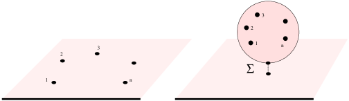
Figure 1: With the help of operator product expansions in the bulk, the computation of $n$-point functions in a boundary theory can be reduced to computing 1-point functions on the half-plane. Consequently, the latter must contain all information about the boundary condition.

The parameters in the 1-point functions are not completely free. In fact, there exist strong sewing constraints on them that have been worked out by several authors [24, 59, 77, 78, 6]. The basic relation can be derived from the following cluster property of correlation functions:

$$\lim_{a\rightarrow\infty}\ \langle\varphi_{1}(z_{1},\bar{z}_{1})\dots\varphi_{P-1}(z_{P-1},\bar{z}_{P-1})\varphi_{P}(z_{P}+a,\bar{z}_{P}+a)\dots\varphi_{N}(z_{N}+a,\bar{z}_{N}+a)\rangle$$ (2.9)

$$= \langle\varphi_{1}(z_{1},\bar{z}_{1})\dots\varphi_{P-1}(z_{P-1},\bar{z}_{P-1})\rangle\ \langle\varphi_{P}(z_{P},\bar{z}_{P})\dots\varphi_{N}(z_{N},\bar{z}_{N})\rangle\ \ .$$

Here, $a$ is a real parameter, and the fields $\varphi_{\nu}=\varphi_{i_{\nu},\bar{\imath}_{\nu}}$ on the right hand side can be placed at $(z_{\nu},\bar{z}_{\nu})$ since the whole theory is invariant under translations parallel to the boundary. If the cluster property is combined with the Ward identities to evaluate 2-point functions of bulk fields, one obtains a constraint of the form

$$A^{\alpha}_{i}\,A^{\alpha}_{j}\ =\ \sum_{k}\ \Xi^{k}_{ij}\ A^{\alpha}_{0}\ A^{\alpha}_{k}\quad\ \ \mbox{ with }\ \ \ A^{\alpha}_{l}\ =\ A^{\alpha}_{l\omega(\bar{l})}\ \ .$$ (2.10)

It holds whenever the vacuum representation “0” occurs in the fusion product of $i$ with $\omega(\bar{\imath})$ and of $j$ with $\omega(\bar{\jmath})$. The coefficient $\Xi^{k}_{ij}$ can be expressed as a combination of the coefficients in the bulk OPE and of the fusing matrix. In some cases, this combination has been shown to agree with the fusion multiplicities or some generalizations thereof (see e.g. [78, 41, 43, 6]). The importance of eq. (2.10) for a classification of boundary conformal field theories has been stressed in a number of publications recently [41, 6, 44] and is further supported by their close relationship with algebraic structures that entered the classification of bulk conformal field theories already some time ago (see e.g. [68, 69, 70]).

Let us remark that, from the string theory point of view, the 1-point functions give the couplings of closed string modes to a D-brane, i.e. generalized tensions and RR-charges. Eq. (2.10) provides an example of non-linear constraints imposed on these couplings.

In our discussion of boundary perturbations, we shall always depart from a set of correlation functions satisfying relation (2.9). Anticipating a more detailed discussion below, we stress that boundary perturbations do not preserve this property in general. One can often interpret the breakdown of rel. (2.9) as a signal for the theory to develop a mixture of different “pure” (i.e. clustering) boundary conditions. Such phenomena are certainly expected to occur upon boundary perturbation and we will present some concrete examples later on.

2.4 Boundary fields.

The action of ${\cal W}$ on the state space of the boundary theory induces a decomposition ${\cal H}=\bigoplus_{i}{\cal V}^{i}$ (possibly with multiplicities) into irreducibles of ${\cal W}$. It also implies that the partition function may be expressed as a sum of characters $\chi_{i}(q)$ of the chiral algebra,

$$Z_{(\Omega,\alpha)}(q)\ :=\ \mbox{\it tr\/}_{\cal H}(q^{L_{0}-c/24})\ =\ \sum_{i}n^{\Omega\alpha}_{i}\,\chi_{i}(q)\ \ \mbox{ where }\ \ n^{\Omega\alpha}_{i}\ \in\ \mathbb{N}\ \ .$$

There exists a one-to-one state-field correspondence $\Phi\equiv\Phi^{(H)}$ between states $\psi\in{\cal H}$ and so-called boundary fields $\psi(x)$ which are defined (at least) for $x$ on the real line [79]. The conformal dimension of a boundary field $\psi(x)$ can be read off from the $L_{0}$-eigenvalue of the corresponding state $\psi\in{\cal H}$. The boundary fields assigned to elements in the vacuum sector ${\cal V}^{0}$ coincide with the chiral fields in the theory, i.e. ${\sf W}(x)=\Phi(w;x)$ for some $w\in{\cal V}^{0}$ and $\Im x=0$. These fields can always be extended beyond the real line and coincide with either $W$ or $\Omega{\overline{W}}$ in the bulk. If other boundary fields admit such an extension, this suggests an enlargement of the chiral algebra in the bulk theory.

Following the standard reasoning in CFT, it is easy to conclude that the bulk fields $\varphi_{ij}(z,\bar{z})$ give singular contributions to the correlation functions whenever $z$ approaches the real line. This can be seen from the fact that the Ward identities describe a mirror pair of chiral charges $i$ and $\omega(j)$ placed on both sides of the boundary. Therefore, the singularities in an expansion of $\varphi(z,\bar{z})\equiv\varphi_{ij}(z,\bar{z})$ around $x={\Re}z$ are given by primary fields which are localized at t $x$ on the the real line, i.e. the boundary fields $\psi(x)$. In other words, the observed singular behaviour of bulk fields $\varphi(z,\bar{z})$ near the boundary may be expressed in terms of a bulk-boundary OPE [24]

$$\varphi(z,\bar{z})\ =\ \sum_{k}\ (2y)^{h_{k}-h-\bar{h}}\ C^{\,\alpha}_{\varphi\;k}\ \psi_{k}(x)\ \ .$$ (2.11)

Here, $\psi_{k}(x)$ are primary fields of conformal weight $h_{k}$, and $z=x+iy$. Which $\psi_{k}$ can possibly appear on the rhs. of (2.11) is determined by the chiral fusion of $i$ and $\omega(j)$, but some of the coefficients $C^{\,\alpha}_{\varphi\,k}$ may vanish for some $\alpha$. One can show that $C^{\,\alpha}_{\varphi\;{0}}=A^{\alpha}_{\varphi}/A^{\alpha}_{0}$; moreover, the $C^{\,\alpha}_{\varphi\;k}$ are related to the 1-point functions by generalizations of the constraints (2.10), see e.g. [59, 78].

In boundary conformal field theory one also considers boundary fields which induce transitions (“jumps”) between different boundary conditions $\alpha,\beta$, see e.g. [22]. These “boundary condition changing operators” are associated with vectors in a state space ${\cal H}_{\alpha\beta}$ depending on both boundary conditions, and they cannot be obtained from bulk fields through a bulk-boundary OPE. Even though we shall only consider homogeneous perturbations of boundary conditions which are constant all along the boundary, we will meet some boundary condition changing operators eventually: At certain values of the deformation parameter $\lambda$, it may happen that a perturbed theory describes a mixture (or superposition) of different clustering boundary conditions. In such cases, no jump is visible along the real axis, but there exist boundary fields which induce transitions between the various “pure” boundary conditions.

Having introduced the boundary fields $\psi(x)$, it is natural to extend the set of correlation functions and to consider correlators in which a number of boundary fields $\psi_{\nu}(x_{\nu})=\Phi(\psi_{\nu},x_{\nu})$ are inserted along with bulk fields:

$$\langle\psi_{1}(x_{1})\dots\psi_{M}(x_{M})\,\varphi_{1}(z_{1},\bar{z}_{1})\dots\varphi_{N}(z_{N},\bar{z}_{N})\rangle_{\alpha}\ \ \ \mbox{ for }\ \ \ x_{\nu}<x_{\nu+1}\ \ \ .$$ (2.12)

These functions are analytic in the variables $z_{\nu}$ throughout the whole upper half-plane $\Im z_{\nu}>0$. For the variables $x_{\nu}$, the domain of analyticity is restricted to the interval $x_{\nu}\in\;]x_{\nu-1},x_{\nu+1}[$ on the boundary. In most cases, there exists no unique analytic continuation of $\psi_{\nu}(x_{\nu})$ to other points on the real axis which lie beyond the insertion points of the neighbouring boundary fields. In fact, if we continue analytically along curves like the one shown in Figure 2, the result will typically depend on whether we move the field $\psi_{\nu}$ around $\psi_{\nu+1}$ in clockwise or anti-clockwise direction. There are certainly exceptions: Chiral fields ${\sf W}(x)$, for example, do possess a unique analytic continuation to $x\in\mathbb{R}\setminus\{x_{\nu}\}$.

Figure 2: The curve $\gamma^{\nu}_{\nu+1}$ along which correlation functions are analytically continued to exchange the position of two neighboring boundary fields. In most cases the result depends on the orientation of the curve.

Based on this discussion on analyticity, we want to introduce a notion of locality that will become important later on: Two boundary fields $\psi_{1}(x_{1})=\Phi(\psi_{1};x_{1})$ and $\psi_{2}(x_{1})=\Phi(\psi_{2};x_{2})$ are said to be mutually local if

$$\Phi(\psi_{1};x_{1})\ \Phi(\psi_{2};x_{2})\ =\ \Phi(\psi_{2};x_{2})\ \Phi(\psi_{1};x_{1})\ \ \ \mbox{ with }\ \ x_{1}<x_{2}\ \ .$$ (2.13)

The equation is supposed to hold after insertion into arbitrary correlation functions, and for the right hand side to make sense it is required that there exists a unique analytic continuation from $x_{1}<x_{2}$ to $x_{1}>x_{2}$.
A boundary field $\psi(x)=\Phi(\psi;x)$ will be called self-local or analytic in the following if it is mutually local with respect to itself. (The second expression is chosen in view of the properties its correlation functions and of perturbations with self-local marginal operators.)
Let us note that the OPE of two mutually local fields contains only pole singularities. In particular, the OPE of a self-local boundary field $\psi$ with conformal dimension $h_{\psi}=1$ is determined up to a constant $K$ to be

$$\psi(x_{1})\,\psi(x_{2})\ =\ \frac{K}{(x_{1}-x_{2})^{2}}\ +\ {\rm reg}\ \ \ \ \mbox{ if }\ \ h_{\Psi}\,=\,1\ \ .$$ (2.14)

Boundary fields ${\sf W}(x)$ from the chiral algebra are the simplest examples of analytic fields. They are not only local with respect to themselves but to all other boundary fields in the theory.

It is crucial for our analysis of D-brane moduli to observe that further (non-chiral) analytic boundary fields $\psi$ can exist depending on the boundary condition under consideration. Unless they belong to some extended chiral symmetry (which means that the original chiral algebra ${\cal W}$ was not chosen to be the maximal chiral symmetry), these self-local boundary fields $\psi$ will not possess a unique analytic continuation into the full upper half-plane. In fact, “moving” the boundary field $\psi$ around the insertion point of a bulk field $\varphi$ (by analytic continuation) can lead to a non-trivial monodromy in general. Whenever this happens, $\psi$ has no chance to be local wrt. all the boundary fields that appear in the bulk-boundary OPE of the bulk field $\varphi$. Consequently, a non-chiral analytic boundary field $\psi$ is only expected to be local wrt. a subset of boundary fields. The latter includes at least the chiral boundary fields ${\sf W}$ in addition to the field $\psi$ itself.

The existence of non-chiral self-local fields is signaled by a partition function $Z_{\Omega\alpha}(q)$ that contains the vacuum character of a $W$-algebra ${\cal W}_{\Omega\alpha}$ extending the chiral algebra ${\cal W}\subset{\cal W}_{\Omega\alpha}$ of the model. We shall see several examples in Section 4.

3 Marginal perturbations of boundary conditions

Our aim is to study perturbations (or deformations) of a boundary condition which are generated by marginal boundary fields. After some general remarks, we describe a class of perturbations – which we call analytic deformations – that are truly marginal to all orders in the perturbation expansion. They are induced by self-local boundary fields of dimension one. Therefore, deformations generated by chiral currents are among them and may serve us to illustrate the more general construction we propose. In the last subsection we investigate arbitrary non-chiral analytic deformations and derive some of their properties which hold to all orders in perturbation theory.

3.1 The general prescription.

Let us start from some boundary conformal field theory with state space ${\cal H}={\cal H}^{(H)}_{(\Omega,\alpha)}$, where $(\Omega,\alpha)$ denotes the boundary condition along the real line. Boundary operators $\psi(x)\in\Phi({\cal H})$ may be used to define a new perturbed theory whose correlation functions are constructed from the unperturbed ones by the formal prescription

$$\langle\,\varphi_{1}(z_{1},\bar{z}_{1})\cdots\varphi_{N}(z_{N},\bar{z}_{N})\,\rangle_{\alpha;\ \lambda\psi}=Z^{-1}\cdot\langle\,I_{\lambda\psi}\,\varphi_{1}(z_{1},\bar{z}_{1})\cdots\varphi_{N}(z_{N},\bar{z}_{N})\,\rangle_{\alpha}$$

$$:= Z^{-1}\sum_{n}\lambda^{n}\int\cdots\int_{x_{i}<x_{i+1}}\frac{dx_{1}}{2\pi}\cdots\frac{dx_{n}}{2\pi}\ \langle\,\psi(x_{1})\cdots\psi(x_{n})\ \varphi_{1}\cdots\varphi_{N}\,\rangle_{\alpha}$$

$$= Z^{-1}\sum_{n}\frac{\lambda^{n}}{n!}\sum_{\sigma\in S_{n}}\int\cdots\int_{\raisebox{-8.53581pt}{$\scriptstyle x_{\sigma(i)}\,<\,x_{\sigma(i+1)}$}}\frac{dx_{1}}{2\pi}\cdots\frac{dx_{n}}{2\pi}\langle\,\psi(x_{\sigma(1)})\cdots\psi(x_{\sigma(n)})\ \varphi_{1}\cdots\varphi_{N}\,\rangle_{\alpha}$$

where $\lambda$ is a real parameter. The second sum in the lowest line runs over all elements in the permutation group $S_{n}$. Since all the $n!$ summands are identical, the last equality is obvious. It shows, however, that the symbol $I_{\lambda\psi}$ in the first line should be understood as a path ordered exponential of the perturbing operator,

$$I_{\lambda\psi}\ =\ P\exp\bigl{\{}\,\lambda S_{\psi}\,\bigr{\}}\ :=\ P\exp\bigl{\{}\,\lambda\int_{-\infty}^{\infty}\psi(x)\,\frac{dx}{2\pi}\,\bigr{\}}\ \ .$$ (3.1)

The normalization $Z$ is defined as the expectation value $Z=(A^{\alpha}_{0})^{-1}\,\langle I_{\lambda\psi}\rangle_{\alpha}$. These expressions deal with deformations of bulk correlators only. If there are extra boundary fields present in the correlation function, the formulas need to be modified in an obvious fashion so that these boundary fields are included in the “path ordering”. A particularly simple example of this type will be discussed shortly, but we refrain from spelling out the general formula here.

To make sense of the above expressions (beyond the formal level), it is certainly necessary to regularize the integrals (introducing UV- and IR-cutoffs) and to renormalize couplings and fields (see e.g. [23] for a discussion of bulk perturbations in 2D conformal field theory). IR divergences are usually cured by putting the system into a “finite box”, i.e., in our case, by studying perturbations of finite temperature correlators; but this will not play any role below. On the other hand, we have to deal with UV divergences. So, let us introduce a UV cutoff $\varepsilon$ such that the integrations are restricted to the region $|x_{i}-x_{j}|>\varepsilon$. Thereby, all integrals become UV-finite before we perform the limit $\varepsilon\rightarrow 0$.

In the following, we consider marginal boundary deformations where the conformal dimension $h$ of the perturbing operator $\psi(x)$ is $h=1$ so that there is a chance to stay at the conformal point for arbitrary values of the real coupling $\lambda$ (we choose $\psi(x)$ to be anti-selfadjoint). If $h\neq 1$, the perturbation will automatically introduce a length scale and one has to follow the renormalization group (RG)-flow to come back to a boundary conformal field theory. For $h>1$, the perturbations are irrelevant so that one ends up with the original boundary theory. For $h<1$, the perturbation is relevant and it is usually quite difficult to say precisely which conformal fix-point one reaches with a given relevant perturbation. Nevertheless, several non-trivial examples have been studied in the literature, see [38, 92, 25, 33, 60, 61] and references therein, partially with the help of the thermodynamic Bethe ansatz.

All these cases, however, share the common feature that (at the RG fix-point) the new conformal boundary theory is associated to the same bulk CFT – since the local properties in the bulk are not affected by the “condensate” along the boundary. Thus, boundary perturbations can only induce changes of the boundary conditions.

To begin our discussion of marginal perturbations with a boundary field $\psi(x)$, let us investigate the change of the two-point function $\langle\psi(x_{1})\psi(x_{2})\rangle_{\alpha}$ of the perturbing field $\psi$ itself under the deformation. Obviously, the first order contribution involves the following sum of integrals:

$$\int_{-\infty}^{x_{1}-\varepsilon}dx\,\langle\psi(x)\psi(x_{1})\psi(x_{2})\rangle_{\alpha}+\int_{x_{1}+\varepsilon}^{x_{2}-\varepsilon}dx\,\langle\psi(x_{1})\psi(x)\psi(x_{2})\rangle_{\alpha}+\int_{x_{2}-\varepsilon}^{\infty}dx\,\langle\psi(x_{1})\psi(x_{2})\psi(x)\rangle_{\alpha}.$$

From the general form of the three point function (with $x_{1}<x_{2}<x_{3}$)

$$\langle\psi(x_{1})\psi(x_{2})\psi(x_{3})\rangle_{\alpha}=\frac{C^{\alpha}_{\psi\psi\psi}}{(x_{1}-x_{2})(x_{1}-x_{3})(x_{2}-x_{3})}\ ,$$

it is easy to see that the first order contribution to the perturbation expansion is logarithmically divergent unless the structure constant $C^{\alpha}_{\psi\psi\psi}$ from the OPE of boundary fields vanishes. The divergence would force the conformal weight of the field $\psi$ away from the initial value $h_{\psi}=1$ as we turn on the perturbation, i.e. the marginal field $\psi$ is not truly marginal unless $C^{\alpha}_{\psi\psi\psi}=0$. If there are several marginal boundary fields in the theory, degenerate perturbation theory gives a somewhat stronger condition: A marginal field $\psi$ is truly marginal only if $C^{\alpha}_{\psi\psi\psi^{\prime}}=0$ for all marginal boundary fields $\psi^{\prime}$ in the theory – cf. e.g. [30] for the bulk case. Eq. (2.14) shows that self-local marginal boundary operators do satisfy this first order condition. One should stress, however, that this is merely a necessary condition. Since it was derived within first order perturbation theory it is by no means sufficient to guarantee true marginality in higher orders of the perturbation series.

3.2 Truly marginal operators.

The first order condition is how far general investigations of marginal bulk perturbations go. Our main aim here is to prove that every self-local marginal boundary operator is indeed truly marginal to all orders and therefore generates a deformation of a boundary CFT. To this end, let us assume that the perturbing marginal field $\psi(x)$ is self-local in the sense discussed at the end of the previous section. Then the above expression for the deformed bulk correlation functions can be rewritten as

$$\langle\,\varphi_{1}(z_{1},\bar{z}_{1})\cdots\varphi_{N}(z_{N},\bar{z}_{N})\,\rangle^{\varepsilon}_{\alpha;\ \lambda\psi}$$

$$= Z^{-1}\sum_{n}\frac{\lambda^{n}}{n!}\int_{-\infty}^{\infty}\cdots\int_{-\infty}^{\infty}\frac{dx_{1}}{2\pi}\cdots\frac{dx_{n}}{2\pi}\langle\,\psi(x_{1})\cdots\psi(x_{n})\ \varphi_{1}\cdots\varphi_{N}\,\rangle_{\alpha}$$

where all integrals are taken over the real line with the regions $|x_{i}-x_{j}|<\varepsilon$ removed as before. Based on the OPE (2.14) of $\psi$, it is not difficult to see that the divergences in $\varepsilon$ from the numerator cancel those from the denominator so that the limit $\varepsilon\to 0$ of the deformed bulk field correlator can be taken. Moreover, as we are dealing with a self-local marginal operator, this limit can be written as

$$\langle\,\varphi_{1}(z_{1},\bar{z}_{1})\cdots\varphi_{N}(z_{N},\bar{z}_{N})\,\rangle_{\alpha;\ \lambda\psi}=\lim_{\varepsilon\to 0}\;\langle\,\varphi_{1}(z_{1},\bar{z}_{1})\cdots\varphi_{N}(z_{N},\bar{z}_{N})\,\rangle^{\varepsilon}_{\alpha;\ \lambda\psi}$$

$$\phantom{xxxxx}= \sum_{n}\frac{\lambda^{n}}{n!}\int_{\gamma_{1}}\cdots\int_{\gamma_{n}}\frac{dx_{1}}{2\pi}\cdots\frac{dx_{n}}{2\pi}\langle\,\psi(x_{1})\cdots\psi(x_{n})\ \varphi_{1}\cdots\varphi_{N}\,\rangle_{\alpha}$$

where $\gamma_{p}$ is the straight line parallel to the real axis with $\Im\gamma_{p}=i\varepsilon/p$, and it can be computed through contour integration. The expression on the right hand side is manifestly finite, and it is independent of $\varepsilon$ as long as $\varepsilon<$ min$(\Im z_{i})$ where $z_{i}$ denote the insertion points of bulk fields. Thus, the above formula allows us to construct the perturbed bulk correlators to all orders in perturbation theory. In particular, it determines the deformation of bulk 1-point functions and hence the deformation of the structure constants $A^{\alpha}_{\varphi}$ which parameterize the possible boundary theories along with the gluing map.

The extension of these ideas to the deformation of boundary correlators meets some obstacles. In fact, formula (3.2) admits for the obvious generalization

$$\langle\,\psi_{1}(u_{1})\cdots\psi_{M}(u_{M})\ \varphi_{1}(z_{1},\bar{z}_{1})\cdots\varphi_{N}(z_{N},\bar{z}_{N})\,\rangle_{\alpha;\ \lambda\psi}$$

$$= Z^{-1}\sum_{n}\frac{\lambda^{n}}{n!}\int_{-\infty}^{\infty}\cdots\int_{-\infty}^{\infty}\frac{dx_{1}}{2\pi}\cdots\frac{dx_{n}}{2\pi}\;\langle\,\psi(x_{1})\cdots\psi(x_{n})\;\psi_{1}\cdots\psi_{M}\;\varphi_{1}\cdots\varphi_{N}\,\rangle_{\alpha}$$

if and only if the boundary fields $\psi_{1},\ldots,\psi_{M}$ are local with respect to the perturbing field $\psi$. As we have argued in the previous section, this is usually a strong constraint on boundary fields. The integrals on the rhs. of eq. (3.2) diverge as $\varepsilon\rightarrow 0$ whenever the iterated OPE of the perturbing field $\psi$ with one of the boundary fields $\psi_{i}$ contains poles of even order. The (renormalized) correlation functions are again obtained through contour integration,

$$\langle\,\psi_{1}(u_{1})\cdots\psi_{M}(u_{M})\ \varphi_{1}(z_{1},\bar{z}_{1})\cdots\varphi_{N}(z_{N},\bar{z}_{N})\,\rangle_{\alpha;\ \lambda\psi}$$

$$= \sum_{n}\frac{\lambda^{n}}{n!}\int_{\gamma_{1}}\cdots\int_{\gamma_{n}}\frac{dx_{1}}{2\pi}\cdots\frac{dx_{n}}{2\pi}\;\langle\,\psi(x_{1})\cdots\psi(x_{n})\;\tilde{\psi}_{1}\cdots\tilde{\psi}_{M}\;\varphi_{1}\cdots\varphi_{N}\,\rangle_{\alpha}$$

where the fields $\tilde{\psi}_{i}$ in the correlator on the right hand side are given by

$$\tilde{\psi}_{i}\ =\ \Bigl{[}e^{\frac{1}{2}\lambda\psi}\,\psi_{i}\Bigr{]}(u_{i}):=\sum_{n=0}^{\infty}{\lambda^{n}\over 2^{n}n!}\;\oint_{C_{1}}\!{dx_{1}\over 2\pi}\cdots\oint_{C_{n}}\!{dx_{n}\over 2\pi}\;\psi_{i}(u_{i})\psi(x_{n})\cdots\psi(x_{1})\ \ ,$$

and $C_{\nu}$ are small circles around the insertion point of $\psi_{i}$. Since the contour integrals on the rhs. pick out simple poles, the fields $\psi_{i}$ and $\tilde{\psi}_{i}$ have the same conformal dimension – $\tilde{\psi}_{i}$ can be regarded as the image of $\psi_{i}$ under a “rotation” generated by the perturbing field $\psi$.

With the help of eq. (3.2) we are able to study the deformation of $n$-point functions of the (self-local) perturbing field $\psi$ itself. Notice that the OPE (2.14) contains no first order poles so that the fields $\tilde{\psi}$ and $\psi$ coincide; in fact, all the contour integrals in eq. (3.2) are zero if there is no bulk field inserted in the upper half-plane. Hence, any perturbative correction to the $n$-point function of $\psi$ vanishes – which implies that self-local marginal field are truly marginal.

3.3 Chiral marginal boundary perturbations.

For the time being, let us restrict to perturbations with local boundary fields ${\sf J}$ taken from the chiral algebra, i.e. we shall analyze perturbations generated by fields assigned to elements in the subspace ${\cal V}^{0}_{1}\subset{\cal H}$. Such fields are local wrt. all bulk and boundary fields, so that eq. (3.2) may be applied to correlators involving arbitrary bulk and boundary fields. Consequently, a complete non-perturbative picture of the deformation can be given, including a proof of the invariance of the partition function.

3.3.1 Deformation of the gluing map.

Our first goal is to describe the effect a marginal perturbation with the boundary current ${\sf J}$ has on the gluing map $\Omega$. To this end, we phrase the content of the gluing condition (2.5) as follows: Suppose we insert the field $W(z+2i\delta)-\Omega{\overline{W}}(\bar{z}-2i\delta)$ with $z=\bar{z}$ into an arbitrary correlation function of the unperturbed theory. Then, by taking the limit $\delta\rightarrow 0^{+}$, we move $W$ and $\Omega{\overline{W}}$ to the boundary until the correlator vanishes at $\delta=0$. Now we want to understand how the presence of the perturbation $P\exp(\lambda S_{J})$ influences this situation. In more formal terms, we need to evaluate the expression

$$0=\lim_{\delta\rightarrow 0}\ Pe^{\lambda S_{J}}\ \ \left(W(z_{\delta})-\Omega{\overline{W}}(\bar{z}_{\delta})\right)$$

$$= \lim_{\delta\rightarrow 0}\ \sum_{n=0}^{\infty}\frac{\lambda^{n}}{n!}\int_{\gamma_{1}}\cdots\int_{\gamma_{n}}\!\frac{dx_{1}}{2\pi}\cdots\frac{dx_{n}}{2\pi}\;{\sf J}(x_{1})\cdots{\sf J}(x_{n})\,\left(W(z_{\delta})-\Omega{\overline{W}}(\bar{z}_{\delta})\right)$$

where we have used $z_{\delta}=z+2i\delta$, $\bar{z}_{\delta}=z-2i\delta$ and inserted the definition of the operator $P\exp(\lambda S_{J})$ underlying formula (3.2). Our next step involves closing the integration contours $\gamma_{i}$ either in the upper or in the lower half-plane. Let us choose the upper half-plane $\Im z>0$ for all contours (the final result is certainly independent of this choice). If there are other bulk fields in the correlator, we split the closed contour into a small circle $C$ around $z_{\delta}$ and a part surrounding the location of all other fields. The latter correlation function vanishes separately for $\delta\rightarrow 0$ due to the “old” gluing conditions, whereas the former part yields the equation

$$0 = \lim_{\delta\rightarrow 0}\ \sum_{n=0}^{\infty}\frac{\lambda^{n}}{n!}\int_{C}\cdots\int_{C}\!\frac{dx_{1}}{2\pi}\cdots\frac{dx_{n}}{2\pi}\;{\sf J}(x_{1})\cdots{\sf J}(x_{n})$$

$$\hskip 85.35826pt\left(\Phi(w\otimes|0\rangle;z_{\delta},\bar{z}_{\delta})-\Phi(|0\rangle\otimes\Omega w;z_{\delta},\bar{z}_{\delta})\right)\ \ .$$

Here, we have described the fields $W$ and $\Omega{\overline{W}}$ in terms of the corresponding states $w,\Omega w\in{\cal V}^{0}$. Now we insert the formula (2.2) for the operator product expansion between ${\sf J}$ and the chiral fields. Only the residues survive the contour integration so that we get

$$\int_{C}\frac{dx}{2\pi}\;{\sf J}(x)\bigl{(}\Phi(w\otimes|0\rangle;z_{\delta},\bar{z}_{\delta})+\Phi(|0\rangle\otimes\Omega w;z_{\delta},\bar{z}_{\delta})\bigr{)}\ =\ i\,\Phi(J_{0}w\otimes|0\rangle;z_{\delta},\bar{z}_{\delta})\ \ .$$

The second term associated with $\Omega{\overline{W}}$ cannot contribute since it is holomorphic in the upper half-plane. Iteration leads to

$$0 = \lim_{\delta\rightarrow 0}\ \sum_{n=0}^{\infty}\frac{(i\lambda)^{n}}{n!}\left(\Phi(J_{0}^{n}w\otimes|0\rangle;z_{\delta},\bar{z}_{\delta})-\Phi(|0\rangle\otimes\Omega w;\bar{z}_{\delta})\right)$$

$$= \sum_{n}\;\bigl{(}\Phi(\exp(i\lambda J_{0})w;z\bigr{)}-\Phi(\Omega w;z)$$

$$= \ e^{i\lambda J_{0}}\,W(z)e^{-i\lambda J_{0}}-\Omega{\overline{W}}(\bar{z})\ \ .$$

Our last step follows from $J_{0}|0\rangle=0$ and the state field correspondence for boundary fields. Conjugation with $\exp(i\lambda J_{0})$ induces an inner automorphism $\gamma_{J}$ of the chiral algebra ${\cal W}$, defined by

$$\gamma_{J}(W)\ :=\ \exp(-i\lambda J_{0})\,W\,\exp(i\lambda J_{0})\ \ \ \mbox{ for all }\ \ \ W\in{\cal W}\ \ .$$

Replacing $W$ by $\gamma_{J}(W)$ in the last line of our short computation, the final result for the change of the gluing conditions under chiral marginal deformations becomes

$$W(z)\ =\ \Omega\circ\gamma_{{\overline{J}}}({\overline{W}})(\bar{z})\ \ \ \mbox{ for }\ \ \ z=\bar{z}\ \ .$$ (3.6)

Observe that $\gamma_{J}$ acts trivially on the Virasoro field because a current zero mode $J_{0}$ commutes with all the modes $L_{n}$. Hence, the gluing condition $T={\overline{T}}$ and those of all other generators $W\in{\cal W}$ that commute with $J_{0}$ remain unchanged under the deformation with ${\sf J}$. These fields then generate the same Ward identities as before the perturbation.

3.3.2 Deformation of the 1-point functions.

We will now analyze the change of 1-point functions under the deformation induced by ${\sf J}$. Our aim is to derive an exact formula for the perturbed 1-point function. To this end, we evaluate the terms in eq. (3.2) order by order in $\lambda$ using the operator product expansion (2.7) between the field $\varphi_{ij}$ and our current ${\sf J}(x)$. Thereby, the calculation of the perturbed 1-point function is essentially reduced to the following simple computation:

$$\langle\varphi_{ij}(z,\bar{z})S_{J}\rangle_{\alpha}=\int_{-\infty}^{\infty}\frac{dx}{2\pi}\,\left(\ \frac{X^{i}_{J}}{x-z}\,\langle\varphi_{ij}(z,\bar{z})\rangle_{\alpha}-\langle\varphi_{ij}(z,\bar{z})\rangle_{\alpha}\,\frac{X_{\Omega{\overline{J}}}^{j}}{x-\bar{z}}\right)$$XXXXX

$$= \int_{-\infty}^{\infty}\frac{dx}{2\pi}\,\left(\frac{X^{i}_{J}}{x-z}\frac{A^{\alpha}_{ij}}{(z-\bar{z})^{2h_{i}}}-\frac{A^{\alpha}_{ij}}{(z-\bar{z})^{2h_{i}}}\frac{X_{\Omega{\overline{J}}}^{j}}{x-\bar{z}}\right)$$

$$= \frac{X_{J}^{i}A^{\alpha}_{ij}}{(z-\bar{z})^{2h_{i}}}\int_{-\infty}^{\infty}\frac{dx}{2\pi}\left(\frac{1}{x-z}-\frac{1}{x-\bar{z}}\right)\ =\ \frac{i\,X_{J}^{i}A^{\alpha}_{ij}}{(z-\bar{z})^{2h_{i}}}\ \ .$$

It involves the same kind of arguments as in the previous subsection and, in addition, the intertwining relation after eq. (2.8). The higher order terms can be computed in the same way and give

$$\langle\varphi_{ij}(z,\bar{z})\rangle_{\alpha:\,\lambda J}\ =\ \frac{e^{i\lambda X_{J}^{i}}A^{\alpha}_{ij}}{(z-\bar{z})^{2h_{i}}}\ \ .$$ (3.7)

Consequently, the effect of the perturbation is to “rotate” the matrix $A^{\alpha}_{ij}$ with $\exp(i\lambda X_{J}^{i})$. This behavior is consistent with the change of the gluing automorphism and the intertwining relation of the linear map $A^{\alpha}_{ij}$.

3.3.3 Partition function and cluster property.

We have argued in the first subsection that correlation functions involving boundary fields can be deformed by the simple prescription (3.2) if all boundary fields in the correlator are local with respect to the perturbing field. In the case of a chiral marginal perturbation, all boundary fields have this property so that formula (3.2) can be used without any restriction on the fields $\psi_{i}$. For correlation functions without insertions of bulk fields, there are no singularities in the upper half-plane. Consequently, the effect of the deformation on pure boundary correlators is trivial. In particular, the conformal weight of all boundary fields is unaffected by the perturbation. Hence, the partition function $Z_{\Omega,\alpha)}(q)$ is invariant under chiral deformations.

Let us also briefly discuss the fate of the cluster property (2.9) under chiral deformations. Without loss of generality, we can restrict ourselves to the investigation of 2-point functions. The basic idea is simple: After expanding the perturbing operator $P\exp(S_{\lambda J})$, we deform the integration contours (which originally are parallel to the real axis) so that they surround the two insertion points $z_{1}$ and $z_{2}$ in the upper half-plane (see Figure 3). Thereby we rewrite the deformed correlation function in each order of the perturbation expansion as a sum of unperturbed 2-point functions involving descendants of the original bulk fields. These functions can be split into products of perturbed 1-point functions by the cluster property of the undeformed theory. This last step involves a standard re-summation, and the details are left to the reader.

Figure 3: For chiral deformations the original curves $\gamma_{p}$ in the contour integrals (3.2) can be deformed into small circles surrounding the insertion points of two bulk fields. The result is expressible through descendants of the original bulk fields.

We will see in the next subsection that our assertions on chiral deformations can be derived rather easily in the boundary state formalism. Here we have chosen an alternative (and certainly more cumbersome) route because it allows for a first illustration of the prescriptions that underlie analytic marginal perturbations. We shall return to more general cases in the last subsection after a brief interlude on the boundary state formalism, which is very effective for chiral marginal deformations but difficult to adapt to other cases.

3.4 The boundary state formalism.

Most aspects of CFTs on the upper half-plane can be studied equally well by introducing boundary states into the “parent” CFT on the full plane – more precisely, on the annulus or on the complement of the unit disk. Boundary states can be viewed as special linear combinations of generalized coherent states (the so-called Ishibashi states), which are placed at the boundary of the annulus resp. disk complement and which provide sources for the bulk fields. This leads to a generalized notion of D-branes coupling to closed string modes [79].

An abstract characterization of a boundary state can be given in terms of bulk field correlation functions: Let us use $z,\bar{z}$ as coordinates on the upper half-plane as before and $\xi,\bar{\xi}$ with

$$\xi\ =\ e^{{{2\pi i}\over{\beta_{0}}}\ln z}\ \ \hbox{\rm and}\ \ \ \bar{\xi}\ =\ e^{-{{2\pi i}\over{\beta_{0}}}\ln\bar{z}}$$ (3.8)

to denote coordinates on the annulus within the full complex plane; $\beta_{0}$ is an inverse “temperature”, i.e. we have identified the semi-circles $|z|=t_{0}$ and $|z|=t_{0}\exp\beta_{0}$ with some positive imaginary time $t_{0}$.

The boundary state $|\alpha\rangle$ which implements a boundary condition $\alpha$ of the boundary CFT (with Hamiltonian $H^{(H)}\,$) into the plane theory (with Hamiltonian $H^{(P)}\,$) is defined by demanding the relation [79]

$$\;{\rm Tr}_{{\cal H}_{\alpha}}\bigl{(}e^{-\beta_{0}H^{(H)}}\varphi^{(H)}_{1}(z_{1},\bar{z}_{1})\cdots\varphi^{(H)}_{N}(z_{N},\bar{z}_{N})\bigr{)}\phantom{XXXXXXXXXXXXXX}$$

$$=\ {\cal J}(z,\bar{z};\xi,\bar{\xi})\cdot\langle\Theta\alpha|\,e^{-{{2\pi^{2}}\over{\beta_{0}}}\,H^{(P)}}\varphi^{(P)}_{1}(\xi_{1},\bar{\xi}_{1})\cdots\varphi^{(P)}_{N}(\xi_{N},\bar{\xi}_{N})\,|\alpha\rangle$$ (3.9)

for arbitrary bulk fields $\varphi^{(H)}_{i}(z_{i},\bar{z}_{i})=\varphi_{i}(z_{i},\bar{z}_{i})$ of the half-plane theory. The Jacobians that appear due to the conformal transformation from $(z_{i},\bar{z}_{i})$ to $(\xi_{i},\bar{\xi}_{i})$ are collectively denoted by ${\cal J}(z,\bar{z};\xi,\bar{\xi})$; $\Theta$ is the CPT-operator. The above definition may be extended so as to allow for two different boundary states $|\alpha\rangle$, $|\beta\rangle$ at the boundaries of the annulus, corresponding to a strip with two different boundary conditions $\alpha,\beta$, or to a jump in the boundary condition along the real line.

There exists an alternative way to introduce boundary states, namely by equating zero-temperature correlators on the half-plane and on the complement of the unit disk in the plane. Since this is useful to compute the variation of 1-point functions under chiral marginal deformations, we present the formulas. With $z,\bar{z}$ as before, we introduce coordinates $\zeta,\bar{\zeta}$ on the complement of the unit disk by

$$\zeta={1-iz\over 1+iz}\quad\quad{\rm and}\quad\quad\bar{\zeta}={1+i\bar{z}\over 1-i\bar{z}}\ ;$$ (3.10)

if $\,|0\rangle$ denotes the vacuum of the bulk CFT, then the requirement

$$\;\langle\,\varphi^{(H)}_{1}(z_{1},\bar{z}_{1})\cdots\varphi^{(H)}_{N}(z_{N},\bar{z}_{N})\,\rangle_{\alpha}\phantom{XXXXxxXXXXXXXxxxxxxX}$$

$$=\ {\cal J}(z,\bar{z};\zeta,\bar{\zeta})\cdot\langle 0|\,\varphi^{(P)}_{1}(\zeta_{1},\bar{\zeta}_{1})\cdots\varphi^{(P)}_{N}(\zeta_{N},\bar{\zeta}_{N})\,|\alpha\rangle$$ (3.11)

defines the same boundary states as before; see e.g. [24, 79].

The concrete construction of boundary states proceeds in two steps: Given a gluing automorphism $\Omega$ of the chiral algebra ${\cal W}$, one first associates Ishibashi states $|i\rangle\!\rangle_{\Omega}$ to each pair $(i,\omega^{-1}(i^{+}))$ of irreducibles that occur in the bulk Hilbert space [56]; $|i\rangle\!\rangle_{\Omega}$ is unique up to a scalar factor (fixed by relation (3.14) below) and implements the gluing map in the sense that

$$\bigl{[}\,W_{n}-(-1)^{h_{W}}\Omega{\overline{W}}_{-n}\,\bigr{]}\,|i\rangle\!\rangle_{\Omega}=0\ .$$ (3.12)

Full boundary states $|\alpha\rangle_{\Omega}\equiv|(\Omega,\alpha)\rangle$ are given as certain linear combinations of Ishibashi states,

$$|\alpha\rangle_{\Omega}=\sum_{i}B^{i}_{\alpha}\,|i\rangle\!\rangle_{\Omega}\ .$$

The complex coefficients $B^{i}_{\alpha}$ are subject to various consistency conditions, most notably to “Cardy’s conditions” arising from world-sheet duality – see [22] for details: The partition function of the boundary theory on a strip can be calculated on the annulus as a transition amplitude between two boundary states,

$$Z_{\alpha\beta}(q)\equiv{\rm tr}_{{\cal H}^{(H)}}\bigl{(}q^{L_{0}^{(H)}-\frac{c}{24}}\bigr{)}=\langle\Theta\beta|\,\tilde{q}^{L_{0}^{(P)}-\frac{c}{24}}\,|\alpha\rangle\ .$$ (3.13)

This is the two-boundary-state generalization of (3.9) without bulk insertions, and $q=\exp(2\pi i\tau)=\exp(-\beta_{0})$, $\tilde{q}=\exp(-2\pi i/\tau)$. The rhs. of eq. (3.13) can be calculated with the help of

$${}_{\Omega}\langle\!\langle j|\,\tilde{q}^{L_{0}^{(P)}-\frac{c}{24}}\,|i\rangle\!\rangle_{\Omega}\ =\ \delta_{i,j}\,\chi^{\cal W}_{i}(\tilde{q})$$ (3.14)

and, on general grounds, the lhs. in the expression (3.13) must be a sum of ${\cal W}$-characters with (positive) integer coefficients. After a modular transformation, this implies Cardy’s non-linear constraints [22] on the coefficients $B^{i}_{\alpha}$. In particular, the boundary “states” should be regarded as labels for sectors, not as elements in some vector space.

With the help of (3.11), one can show [24, 79] that there is a simple relation to the 1-point functions and structure constants of the bulk-boundary OPE – which are subject to further non-linear sewing constraints like (2.10) – namely

$$A_{i,\omega^{-1}(i^{+})}^{\alpha}=B^{i^{+}}_{\alpha}\quad\ \ \mbox{and}\ \quad C^{\,\alpha}_{\varphi\;0}\ =\ \frac{B^{i^{+}}_{\alpha}}{B^{0}_{\alpha}}\ .$$ (3.15)

The decomposition of a boundary state into Ishibashi states contains the same information as the set of 1-point functions and therefore specifies the “descendant” boundary CFT of a given bulk CFT completely.

Now let us exploit the boundary state formalism for the discussion of marginal boundary perturbations by $W$-algebra currents $J(x)$. To this end, we use eqs. (3.9) or (3.11) to transport the perturbation from the boundary of the upper half-plane to the boundary of the annulus resp. unit disk. This is possible since $J$ is a local field of the bulk theory so that its image under the conformal transformation acts on the state space of the bulk theory. With (3.10) and $h_{J}=1$, we obtain

$$\int_{\mathbb{R}}\frac{dx}{2\pi}\,J^{(H)}(x)=\int_{|\zeta|=1}\!\frac{d\zeta}{2\pi}\,J^{(P)}(\zeta)=iJ^{(P)}_{0}\ .$$ (3.16)

An analogous formula results from the map (3.8) to the annulus, this time the rhs. consists of one integral for each boundary component at $|\xi|=1$ resp. $|\xi|=\frac{2\pi^{2}}{\beta_{0}}\,$. Since chiral currents are analytic, we need not worry about possible divergences, as they can be avoided by deforming the integration contour.

It is the last equality in (3.16) that makes it easy to treat perturbations by chiral currents in the boundary state formalism: We could not conclude that $\int_{\mathbb{R}}\!dx\,J^{(H)}(x)=J^{(H)}_{0}$ on the half-plane because of the different integration contour in the definition of half-plane modes, see [20, 21, 79]. Using boundary states, however, the effect of marginal boundary perturbations on a half-plane theory reduces to the action of current zero modes – as long as the perturbing fields are taken from the chiral algebra.

The boundary states which describe the boundary conditions before and after the chiral perturbation are related by a simple “rotation”. Correlators of the deformed boundary CFT can be obtained upon replacing $|\alpha\rangle$ in the correspondences (3.9) or (3.11) by

$$|(\Omega,\alpha)\rangle_{\lambda\,J}\equiv|(\Omega,\alpha)\,;\,{\lambda\,J}\rangle\ \;=\ \,e^{i\lambda J_{0}}\,|(\Omega,\alpha)\rangle\$$ (3.17)

where $J_{0}\equiv J^{(P)}_{0}$ is the zero mode of the left-moving current on the plane.

We have made the unperturbed gluing map $\Omega$ explicit in (3.17). Indeed, from this formula, we can immediately re-derive the change (3.6) of the gluing conditions under the marginal deformation by $J(x)$: Using that left- and right-movers commute, as well as the simple relation $J_{n}\,|(\Omega,\alpha)\rangle=-\,\Omega{\overline{J}}_{-n}\,|(\Omega,\alpha)\rangle$, eq. (3.12) gets replaced by

$$\bigl{[}\,W_{n}-(-1)^{h_{W}}\,\Omega\circ\gamma_{{\overline{J}}}\,\bigl{(}{\overline{W}}_{-n}\bigr{)}\,\bigr{]}\,|(\Omega,\alpha)\rangle_{\lambda\,J}\ =\ 0\ \vspace*{2mm}$$ (3.18)

with $\gamma_{{\overline{J}}}({\overline{W}}):=\exp(-i\lambda{\overline{J}}_{0})\,{\overline{W}}\,\exp(i\lambda{\overline{J}}_{0})$; see also [49] for special cases of (3.18). Likewise, eq. (3.7) for the change of the 1-point functions follows from (3.11), (3.15) and (3.17).

Finally, let us use the boundary state formalism to verify – without resorting to perturbative arguments – that the partition function $Z_{\alpha}(q)\equiv Z_{\alpha\alpha}(q)$ of a boundary CFT with boundary condition $\alpha$ along the real line stays invariant under marginal perturbations by a chiral boundary field $J(x)$: We have to compute the transition amplitude between $|\alpha;\,\lambda\,J\rangle$ and $\langle\Theta\,(\alpha;\,\lambda\,J)\,|$. But this equals the unperturbed amplitude $Z_{\alpha\alpha}(q)$ because $\langle\Theta\,\exp(i\lambda J_{0})\,\alpha|=\langle\Theta\alpha|\,\exp(-i\lambda J_{0})$ and because $\exp(i\lambda J_{0})$ commutes with $L^{(P)}_{0}$. The spectrum of the boundary theory does not change.

Up to now, we have always started from a boundary CFT with a constant boundary condition $\alpha$ along the real line and considered boundary perturbations involving marginal fields that were integrated over the whole boundary – which corresponds to simultaneous deformation of one and the same boundary state $|\alpha\rangle$ on both ends of the annulus. Generalizations of this would involve jumps in the boundary conditions along the real line and different boundary operators integrated over the segments of constant boundary condition.

The boundary state formalism allows to discuss the basic case with one such jump, using different perturbations for (possibly different) in- and out-boundary states in equations (3.9,3.17). Generically, the partition functions $Z_{(\alpha;\lambda_{1}J^{1}),(\beta;\lambda_{2}J^{2})}(q)$ for such systems will show a different spectrum than in the unperturbed situation, and they will involve “twisted characters” of the symmetry algebra – more precisely, characters of representations twisted by inner automorphisms Ad_U with $U=\exp\{i(\lambda_{1}J^{1}_{0}-\lambda_{2}J^{2}_{0})\}$. We shall take advantage of this fact in Section 4.

3.5 Non-chiral analytic perturbations.

Let us now turn towards deformations generated by marginal boundary fields $\psi(x)$ that are self-local (in the sense of Section 2.4) but not taken from the chiral algebra. We have seen already that these fields are truly marginal to all orders in $\lambda$, so we can ask how gluing conditions and 1-point functions behave under finite perturbations. We will settle the former issue completely in 3.5.1 and make some general statements on 1-point-functions and on the spectrum in Subsection 3.5.2.

3.5.1 Change of the gluing map.

As in the case of chiral boundary perturbations, we would like to study the effect of non-chiral marginal deformations on the gluing conditions $W=\Omega({\overline{W}})$ for the generators of the observable algebra ${\cal W}$. We start the discussion by showing that $T={\overline{T}}$ is not changed under analytic deformations to all orders of $\lambda$.

This follows essentially from the OPE between ${\sf T}(z)$ and $\psi(x)$: For a field $\psi$ of conformal dimension $h=1$, the singular part of the OPE is a total derivative,

$${\sf T}(z)\,\psi(x)\ =\ \frac{1}{(z-x)^{2}}\,\psi(x)+\frac{1}{z-x}\,\partial_{x}\psi(x)\ +\;{\rm reg}\ =\ \partial_{x}\ \left(\frac{1}{z-x}\,\psi(x)\right)\ +\;{\rm reg}\ \ .\ \$$

We can test the gluing condition for the Virasoro field by inserting $T(z)$ into the correlation function (3.2) such that $\Im z>\varepsilon$, and then moving $T(z)$ down towards the real axis, where it can be compared to ${\overline{T}}(\bar{z})$. While passing through one of the contours $\gamma_{i}$, we pick up a term

$$\int_{C}\frac{dx}{2\pi}\ {\sf T}(z)\,\psi(x)\ =\ \int_{C}\frac{dx}{2\pi}\ \partial_{x}\,\left(\frac{1}{z-x}\,\psi(x)\right)\ =\ 0$$

where $C$ is a small circle surrounding the insertion point of the Virasoro field. The contour integral along $C$ vanishes, which means that the Virasoro field $T$ cannot feel the presence of the perturbation and hence the gluing condition stays intact.

The previous argument can be generalized to the following simple criterion:
Under analytic deformation with a self-local perturbing field $\psi(x)$, a prescribed gluing condition for a chiral field $W(z)$ stays invariant to all orders in $\lambda$ if the singular part of the OPE $\;W(z)\,\psi(x)\,$ is a total derivative with respect to $x$.
We will encounter several examples later in the text. Let us remark that the same criterion is at least necessary for other (non-analytic) marginal perturbations to preserve a given gluing condition.

Perturbations with currents ${\sf J}$ from the chiral algebra often lead to a non-trivial deformation (3.18,3.6) of the gluing condition of a symmetry generator $W(z)$, without destroying the associated Ward identity. We will see that this is impossible for non-chiral analytic deformations: In Subsection 3.3.1, the change in the $W(z)$-gluing condition was obtained by moving the chiral field $W(z)$ through the stack of integration contours. After a bit of combinatorics, the same procedure for non-chiral analytic deformations results in

$$W(z)\,e^{\lambda\!\int\!{dx\over 2\pi}\,\psi(x)}=e^{\lambda\!\int\!{dx\over 2\pi}\,\psi(x)}\,\Bigl{[}e^{\lambda\psi}\,W\Bigr{]}(z)$$

(to be understood in the limit $z\rightarrow\bar{z}$) with

$$\Bigl{[}e^{\lambda\psi}\,W\Bigr{]}(z):=\sum_{n=0}^{\infty}{\lambda^{n}\over n!}\;\oint_{C_{1}}\!{dx_{1}\over 2\pi}\cdots\oint_{C_{n}}\!{dx_{n}\over 2\pi}\;W(z)\,\psi(x_{1})\cdots\psi(x_{n})\ \ .$$ (3.19)

The curves $C_{i}$ encircle the point $z$ in the upper half-plane as in Figure 3. To each order $n$, the integrals will pick some term $\psi^{(n)}$ from the OPE of $W(z)$ with the product of perturbing fields. At least part of the $\psi^{(n)}$ are true boundary fields which are not defined away from the boundary, thus they do not belong to the chiral algebra and the above gluing does not produce Ward identities for $W(z)$ in the deformed boundary CFT.

This shows that a non-chiral analytic perturbation either breaks or leaves invariant the Ward identity associated to a given generator of ${\cal W}$. In general, this leads to a new conformally invariant boundary theory with Ward identities governed by a subalgebra ${\cal U}$ of the original chiral algebra ${\cal W}$.

Let us add a few comments on deformations of boundary conditions for $N=2$ superconformal CFTs because they constitute an important motivation for the present work and because they nicely illustrate the criterion given above. In such theories, one considers two types (A,B) of gluing conditions for the chiral fields $G^{\pm},J,T$,

A-type: $$J(z)\ =\ -{\overline{J}}(\bar{z})\ \ ,\ \ G^{\pm}(z)\ =\eta\,\overline{G}{}^{\mp}(\bar{z})$$ (3.20)

B-type: $$J(z)\ =\ \ {\overline{J}}(\bar{z})\ \ ,\ \ G^{\pm}(z)\ =\ \eta\,\overline{G}{}^{\pm}(\bar{z})$$ (3.21)

supplemented by $T={\overline{T}}$ in both cases. The parameter $\eta$ is restricted in order to have a supersymmetric “space-time” theory. More precisely, one requires that an $N=1$ subalgebra with generating supercurrent $G(z):=G^{+}(z)+G^{-}(z)$ or $G^{\prime}(z):=i(G^{+}(z)-G^{-}(z))$ is preserved by any boundary condition. This leaves us with the choice $\eta=\pm 1$. The gluing conditions (3.20,3.21) were first introduced in [66], where the connection with supersymmetric cycles in Calabi-Yau manifolds was investigated. A quite non-trivial realization in CFTs associated with homogeneous spaces was constructed in [89].

It is natural to try and deform an $N=2$ superconformal boundary CFT with the chiral U(1) current. According to our general formulas, such deformations lead to

$$\mbox{A type:}\ \ \ G^{\pm}(z)\ =\ e^{-i\lambda}\eta\,\overline{G}^{\mp}(\bar{z})\ ,\ \quad\ \mbox{B type:}\ \ \ G^{\pm}(z)\ =\ e^{i\lambda}\eta\,\overline{G}^{\pm}(\bar{z})\ .$$

This however, spoils the condition $\eta=\pm 1$ and hence the “space-time” supersymmetry unless $\lambda$ is a multiple of $\pi$. Thus there is no family of supersymmetric boundary CFTs generated by perturbing an $N=2$ model by the U(1) boundary current $J$.

On the other hand, marginal deformations associated with chiral or anti-chiral primaries can exist and preserve $N=2$ supersymmetry. A state $|\psi_{c,a}\rangle$ (or the corresponding conformal field) in an $N=2$ superconformal field theory is called chiral resp. anti-chiral primary if it satisfies

$$G^{+}_{-{1\over 2}}\,|\psi_{c}\rangle=0\quad\quad{\rm resp.}\ \ \quad G^{-}_{-{1\over 2}}\,|\psi_{a}\rangle=0\ .$$

It follows that $|\psi_{c,a}\rangle$ are $N=2$ highest weight states with charge and dimension related as $q=2h$ resp. $q=-2h$, see [58].

Suppose there is a chiral primary boundary field $\psi_{c}(x)$ of conformal dimension $1/2$ in an $N=2$ boundary CFT, and set $\psi(x):=G^{-}_{-1/2}\psi_{c}(x)-G^{+}_{-1/2}\psi_{a}(x)$ where $\psi_{a}(x)=\bigl{(}\psi_{c}(x)\bigr{)}^{*}$ is the anti-chiral conjugate of $\psi_{c}(x)$. Then $\psi(x)$ is anti-selfadjoint, uncharged and marginal, and we can study the deformations it induces.

Typically, there will be other boundary and bulk operators that are non-local wrt. $\psi(x)$, so we have to rely on the methods developed for non-chiral perturbations. The gluing condition for the Virasoro field is preserved because of $h_{\psi}=1$ (see above). Since $\psi(x)$ carries no charge, the singular contribution to the operator product of the current ${\sf J}(w)$ with $\psi(x)$ vanishes so that the gluing condition for the current $J$ is untouched. As for the supercurrents ${\sf G}^{\pm}(z)$, we use the state-field correspondence and the $N=2$ relations to find

$${\sf G}^{-}(z)\,\Bigl{(}G^{-}_{-{1\over 2}}\psi_{c}\Bigr{)}(x)\ \sim\ 0\ \ ,\ \ \ {\sf G}^{+}(z)\,\Bigl{(}G^{-}_{-{1\over 2}}\psi_{c}\Bigr{)}(x)\ \sim\ \partial_{x}\,\Bigl{(}{2\,\psi_{c}(x)\over z-x}\Bigr{)}\$$

together with the analogous relations for the anti-chiral contribution $G^{+}_{-1/2}\psi_{a}(x)$ to the perturbing field $\psi$. The first equation already holds when $\psi_{c}(x)$ is any $N=2$ primary, whereas in the second it is crucial that $\psi_{c}(x)$ is chiral. Our general criterion shows that deformations with $\psi(x)$ do not affect the prescribed $N=2$ gluing conditions – whether they are of A-type or of B-type – to first order in the perturbation parameter; hence they are invariant to all orders if $\psi(x)$ is a self-local marginal field.

Deformations induced by chiral primaries as above could serve as a starting point to define topological $N=2$ boundary CFTs. In the bulk case [31, 91], topological field theories yield families of commutative associative rings, parameterized by the perturbation parameter, which often can be interpreted as quantum cohomology rings of complex manifolds. It would be interesting to see which new structures arise from topological boundary correlators. Since the topology of the “supporting space”, i.e. of the world-sheet boundary, does not allow to continuously interchange arguments in correlation functions, one may expect that non-commutative rings appear quite naturally.

3.5.2 One-point-functions, spectrum, and the cluster property.

A boundary conformal field theory is determined by the gluing conditions and the 1-point functions. We have discussed the change of gluing conditions under non-chiral analytic deformations, but it is difficult to obtain general statements on the deformed 1-point functions, in particular because they are to be computed for all primary fields of the smaller (“unbroken”) subalgebra ${\cal U}\subset{\cal W}$ associated to the reduced set of Ward identities that may survive after turning on the perturbation. Nevertheless, as we will see later on, there are examples of non-trivial analytic deformations for which the deformed 1-point functions can be constructed to all orders.

At the moment, we limit ourselves to a simple first order criterion for the invariance of a 1-point function. Let $\varphi(z,\bar{z})$ be an arbitrary quasi-primary bulk field, e.g. a primary field for the reduced chiral algebra ${\cal U}\subset{\cal W}$. Conformal transformation properties fix the 2-point function of $\varphi(z,\bar{z})$ with the perturbing field $\psi(x)$ up to a constant,

$$\langle\varphi(z,\bar{z})\psi(x)\rangle_{\alpha}\ =\ \frac{C^{\alpha}_{\varphi\psi}}{(z-\bar{z})^{2h-1}(z-x)(\bar{z}-x)}\ \ .$$

Here, $h=\bar{h}$ is the conformal weight of the field $\varphi$, and the bulk-boundary OPE coefficient $C^{\alpha}_{\varphi\psi}$ depends on the original boundary condition $\alpha$. By the residue theorem, we get the following first order correction for the perturbed 1-point function

$$\langle\varphi(z,\bar{z})\rangle_{\alpha;\,\lambda\psi}\ =\ \langle\varphi(z,\bar{z})\rangle_{\alpha}+i\,\lambda\,\frac{C^{\alpha}_{\varphi\psi}}{(z-\bar{z})^{2h}}+O(\lambda^{2})\ \ .$$ (3.22)

To leading order, a 1-point function $\langle\varphi(z,\bar{z})\rangle_{\alpha}$ is invariant under a perturbation with $\psi$ if and only if $C^{\alpha}_{\varphi\psi}=0$. Again this is a necessary condition for the invariance of a given 1-point function under any truly marginal perturbation, but it is certainly not sufficient.

A full computation of the partition function requires complete knowledge of all 1-point functions and hence it is at best accessible through a case by case study. On the other hand, there are some general statements we can make about the behaviour of $Z_{\alpha}(q)$ under analytic deformations. We have argued above that the formula (3.2) can be used to construct perturbed correlators of boundary fields $\psi_{i}$ which are local with respect to the perturbing field $\psi$. By the same arguments as in chiral deformation theory, we conclude that the conformal weights of such fields $\psi_{i}$ are invariant under the deformation. While this criterion does not protect the full spectrum of boundary conformal weights (as in the case of chiral deformations where all boundary fields are local with respect to $\psi$), it shows that part of the partition function stays intact. In particular, all chiral fields ${\sf W}$ are local with respect to $\psi$ so that the partition function will always contain the vacuum character of the original chiral algebra ${\cal W}$ even if gluing conditions and Ward identities are broken down to a subalgebra ${\cal U}\subset{\cal W}$. Furthermore, while the “gluing” (3.19) of a chiral field $W(z)$ to boundary operators destroys the Ward-identity for $W(z)$, it still leads to a (possibly twisted) action of the full chiral algebra ${\cal W}$ on the state space ${\cal H}$. This effect can be read off from the partition function of the deformed theory which still decomposes into characters of (twisted) representations of ${\cal W}$, see the examples below.

The cluster property is somewhat more difficult to attack. Note that the argument at the end of Subsection 3.3.3 cannot be used in this simple form because the deformed correlators are not expressible through correlators of descendants of the original bulk fields. There exists a variant of the previous reasoning which takes into account the specific analyticity properties of correlators with insertions of self-local non-chiral boundary fields and bulk fields. Its convergence behaviour in the limit $n\rightarrow\infty$, however, is not easy to control. It is likely that the cluster property is preserved for an open neighbourhood of $\lambda=0$ but is bound to break down at certain finite values of the perturbation parameter $\lambda$ whenever we deform with some non-chiral boundary fields. This agrees with the examples we analyse below. Often, the breakdown of the cluster property has an interesting physical or geometric interpretation.

4 Example: Boundary deformations for c = 1 theories

The results of the previous section hold for arbitrary boundary CFTs. We will now illustrate them in a simple example, namely the free bosonic field. To begin with, we present the uncompactified theory with Neumann and Dirichlet boundary conditions and study their deformations. Then the same analysis is made for the compactified boson. In the third subsection, we investigate boundary perturbations of $c=1$ orbifold theories. Although the models under consideration are simple enough, we will encounter rich patterns in the brane moduli space, including some unexpected phenomena.

4.1 The uncompactified theory.

The dynamical degrees of freedom of the bulk theory are obtained from a single field $X(z,\bar{z})$ which obeys the usual equation of motion $\partial\bar{\partial}X(z,\bar{z})=0$. The modes of the left- and right-moving chiral currents $J(z)=2i\,\partial X(z,\bar{z})=\sum\,a_{n}\,z^{-n-1}$ and ${\overline{J}}(\bar{z})=2i\,\bar{\partial}X(z,\bar{z})=\sum{\bar{a}}_{n}\,\bar{z}^{-n-1}$ generate a U(1)$\,\times\,$U(1) algebra with canonical commutation relations

$$[\,a_{n}\,,\,a_{m}\,]\ =\ n\,\delta_{n,-m}\ \ ,\ \ [\,{\bar{a}}_{m}\,,\,{\bar{a}}_{m}\,]\ =\ n\,\delta_{n,-m}\ \ .$$

The Virasoro fields are obtained from $J,{\overline{J}}$ by normal-ordering, $T(z)=\frac{1}{2}\,{\bf:}\,J\,J\,{\bf:}\,(z)$ and ${\overline{T}}(\bar{z})=\frac{1}{2}\,{\bf:}\,{\overline{J}}\,{\overline{J}}\,{\bf:}\,(\bar{z})\;$.
The abelian current algebra has irreducible representations ${\cal V}^{g}$ labeled by real numbers $g$, the U(1) charge. ${\cal V}^{g}$ is generated from a ground state $|g\rangle$ with the properties

$$a_{n}\;|g\rangle\ =\ 0\ \ \mbox{ for all }\ \ n>0\ \ \ \mbox{ and }\ \ a_{0}\;|g\rangle\ =\ g\;|g\rangle\ \ .$$

The lowest-energy subspace $V^{g}_{0}$ of ${\cal V}^{g}$ is one-dimensional and spanned by $|g\rangle$, the element $a_{0}$ acts on $V^{g}_{0}$ by $X^{g}_{J}=g$.

Putting things together, one can realize the bosonic field $X$ on the state space ${\cal H}^{(P)}=\bigoplus_{g}{\cal V}^{g}\otimes{\cal V}^{g}$ which is a diagonal sum with equal U(1) charges for both chiralities. In the explicit formula

$$X(z,\bar{z})\ =\ x-\frac{i}{4}\,p\,\ln(z\bar{z})+\frac{i}{2}\sum_{n\neq 0}\,\left(\frac{a_{n}}{n}\,z^{-n}+\frac{{\bar{a}}_{n}}{n}\,\bar{z}^{-n}\right)\ ,$$

one new element $x$ appears which acts as differentiation $x=i\partial_{g}$ on the state space. We have also introduced the operator $p=a_{0}+{\bar{a}}_{0}$ which has the usual Heisenberg commutation relation with $x$. Bulk fields $\varphi_{g_{1}g_{2}}(z,\bar{z})$ exist only for $g_{1}=g_{2}$ so that we will omit one index in the following. $\varphi_{g}=\varphi_{gg}$ is obtained from the bosonic field by

$$\varphi_{g}(z,\bar{z})\ =\ {\bf:}\,\exp(2igX(z,\bar{z}))\,{\bf:}\ \ ,$$

and with proper normal-ordering these fields can be shown to obey the operator product expansions

$$\varphi_{g_{1}}(z_{1},\bar{z}_{1})\ \varphi_{g_{2}}(z_{2},\bar{z}_{2})\ \sim\ |z_{1}-z_{2}|^{2g_{1}g_{2}}\varphi_{g_{1}+g_{2}}(z_{2},\bar{z}_{2})+\dots\ \ .$$

The conformal weights $h_{g}=\bar{h}_{g}$ of $\varphi_{g}(z,\bar{z})$ are given by $h_{g}=\frac{1}{2}g^{2}$.

We will look for boundary conditions that preserve the chiral symmetry algebra generated by the U(1) current $J$. There are two possibilities for the gluing map which we can use:

$$\mbox{Neumann boundary condition:}\ \ \ \ \ \ J(z) = \Omega_{N}{\overline{J}}(\bar{z})\ \equiv\ \ {\overline{J}}(\bar{z})\$$ (4.1)

$$\mbox{Dirichlet \ boundary condition:}\ \ \ \ \ \ J(z) = \Omega_{D}{\overline{J}}(\bar{z})\ \equiv\ -{\overline{J}}(\bar{z})\$$ (4.2)

The Neumann type boundary conditions are realized by a bosonic field

$$X(z,\bar{z})\ =\ x-\frac{i}{4}\,p\,\ln(z\bar{z})+\frac{i}{2}\sum_{n\neq 0}\,\frac{a_{n}}{n}\ \left(\,z^{-n}+\bar{z}^{-n}\,\right)$$

acting on a state space ${\cal H}=\bigoplus_{g}{\cal V}^{g}$. Here, $x=i\partial_{g}$ as before, and $a_{n}$, $p=2a_{0}$ are the modes of the generator ${\sf J}$ of the U(1) symmetry in the boundary Hilbert space. The computation of the 1-point function of $\varphi_{g}(z,\bar{z})=\;{\bf:}\,\exp(2igX(z,\bar{z}))\,{\bf:}$ is a straightforward exercise, leading to

$$\langle\varphi_{g}(z,\bar{z})\rangle_{N}\ =\ \delta_{g,0}\ \ .$$

Note that there appears no free parameter in these 1-point functions, i.e. there is only one boundary theory with Neumann boundary conditions for an uncompactified free boson.

For Dirichlet boundary conditions, we build the bosonic field according to

$$X(z,\bar{z})\ =\ x_{0}+\frac{i}{2}\sum_{n\neq 0}\,\frac{a_{n}}{n}\ \left(z^{-n}-\bar{z}^{-n}\right)\ \ .$$

Here, $x_{0}$ is a free real parameter describing the value of the bosonic field along the boundary, i.e. $X(z,\bar{z})\equiv X(z)+X(\bar{z})=x_{0}$ for $z=\bar{z}$. The field $X$ acts on a state space ${\cal H}={\cal V}^{0}$ consisting only of the vacuum representation. This time, calculation of 1-point functions for $\varphi_{g}(z,\bar{z})$ results in the formula

$$\langle\varphi_{g}(z,\bar{z})\rangle_{D\,x_{0}}\ =\ \frac{e^{2igx_{0}}}{(z-\bar{z})^{2h_{g}}}\ \$$

which depends on $x_{0}$, parameterizing different possible boundary theories with Dirichlet boundary conditions.

Note that, for the free boson theory, the structure constants $\Xi$ in the sewing constraint (2.10) are given by $\Xi^{g^{\prime}}_{g_{1},g_{2}}=\delta_{g^{\prime},g_{1}+g_{2}}$. The numbers $A^{x_{0}}_{g}=\exp(2igx_{0})$ solve eq. (2.10) and hence the theory has the cluster property (2.9); at the same time, this means that superpositions (“mixtures”) of “pure” Dirichlet boundary conditions do not cluster.

4.1.1 Chiral deformations.

Let us now study marginal deformations and start with the chiral current ${\sf J}$ which is the only field of weight $h=1$ in the chiral algebra. Since the zero mode $a_{0}$ commutes with all other elements in ${\cal W}$, it generates the trivial inner automorphism $\gamma_{J}=id$ on the chiral algebra. It follows then from eq. (3.6) that the gluing conditions are invariant under the deformation, i.e.  they are given by the formulas (4.1,4.2) for all values of the perturbation parameter $\lambda$. Consequently, the only possible effect of the perturbation on the boundary theories is due to changes of the 1-point functions.

For Neumann boundary conditions we have $A^{N}_{g}=\delta_{g,0}$ so that, according to our formula (3.7), this coefficient – and therefore the Neumann boundary theory – stays invariant under deformations with ${\sf J}(x)$. For Dirichlet boundary conditions, things are a bit more interesting. The coefficients $A^{x_{o}}_{g}=e^{2igx_{0}}$ of the Dirichlet boundary condition behave as

$$A^{x_{0}}_{g}\ \longrightarrow\ e^{i\lambda g}\,e^{2igx_{0}}\ =\ e^{2ig(x_{0}+\frac{\lambda}{2})}\ \$$

when we turn on the perturbation. As a result of the deformation, the parameter $x_{0}$ gets shifted by $\lambda/2$ – i.e. the D-brane is displaced.

4.1.2 Non-chiral deformations.

In the case of Neumann boundary conditions, there are two other boundary fields of conformal dimension $h=1$. We will consider perturbations by the combinations

$$\psi^{1}(x)\ :=\ \sqrt{2}\,\cos\{2\sqrt{2}X(x)\}\ \ \ \ \ \mbox{ and }\\ \ \ \ \psi^{2}(x)\ :=\ \sqrt{2}\,\sin\{2\sqrt{2}X(x)\}\ ,$$

which will be seen to break the chiral symmetry down to the Virasoro algebra by inducing a periodic “potential” along the boundary. This has been studied in some detail in [15, 17, 76].

The boundary fields $\psi^{a}(x)$, $a=1,2$, are local with respect to themselves. By our general considerations of Section 3.2 on analytic perturbations, $\psi^{a}(x)$ are truly marginal (to all orders in the “coupling” $\lambda$). At the same time, we expect the spectrum of boundary fields to change when the boundary potential is turned on, because the boundary Hilbert space ${\cal H}=\bigoplus_{g}{\cal V}^{g}$ of the Neumann theory contains fields which are non-local wrt.  $\psi^{a}(x)$ – in fact, only the scaling dimensions of operators with charges in $\sqrt{2}\mathbb{Z}$ are protected.

Let us first see how the U(1) gluing conditions behave under perturbations with e.g. $\psi^{1}(x)$. The criterion for invariance of $\Omega$ given in Section 3.5 required that the singular part of the OPE between a chiral symmetry generator $W(z)$ and $\psi^{1}(x)$ is a total $\partial_{x}$-derivative. This is true for the Virasoro field $W(z)=T(z)$, but not for the current $W(z)=J(z)$. So we have to determine the effect of pushing $J(z)$ through the $x_{i}$-integration contour when moving the field towards the real line, in order to evaluate (3.19) describing the change of $J(z)=\overline{J}(\bar{z})$. The OPE of $J(z)$ with $\psi^{1}(x)$ is given by

$$J(z)\,\psi^{1}(x)\ =\ {i\sqrt{2}\over z-x}\,\psi^{2}(z)\ +\ {\rm reg}$$ (4.3)

so that we pick up a term $i\sqrt{2}\psi^{2}(z)$ whenever $J(z)$ passes one of the contours. The effect of moving the field $\psi^{2}(z)$ towards the real axis is determined by the OPE

$$\psi^{2}(z)\,\psi^{1}(x)\ =\ {-i\sqrt{2}\over z-x}\,J(z)+\ {\rm reg}\ \ .$$ (4.4)

We can now apply our general formula (3.19) to derive the following closed expression for the $\psi^{1}$-deformed gluing conditions:

$$J(z)\ =\ \sin(\sqrt{2}\lambda)\,\psi^{2}(x)+\cos(\sqrt{2}\lambda)\,\overline{J}(\bar{z})$$ (4.5)

for $z=\bar{z}=x$. By the same reasoning, one can determine the effect of perturbations with $\psi^{2}$ on the Neumann gluing condition:

$$J(z)\ =\ -\sin(\sqrt{2}\lambda)\,\psi^{1}(x)+\cos(\sqrt{2}\lambda)\,\overline{J}(\bar{z})\ .$$ (4.6)

These equations, which were also found in [17], mean that the boundary reflects left-moving into right-moving currents only at the expense of marginal boundary fields. As a consequence, the correlation functions of the perturbed boundary CFT no longer obey Ward identities for the U(1) current ${\sf J}$. Exceptions occur whenever $\lambda=n\,{\pi\over\sqrt{2}}$ for some integer $n$: Then $\psi^{a}(x)$ disappear from (4.5,4.6) and, if $n$ is odd, the original Neumann conditions for $J(z)$ are turned into Dirichlet conditions. We will refer to the latter values of the perturbation parameter as Dirichlet-like points.

Broken U(1) symmetry complicates computations considerably. Since it is only the Virasoro algebra that remains at our disposal, we have to characterize the deformed theory through the 1-point functions of all Virasoro primary fields. The decomposition of irreducible U(1) modules into $c=1$ Virasoro modules is well known. Both coincide as long as the conformal dimension of the primary field is not given by $h={m^{2}}$ for any $m\in\frac{1}{2}\mathbb{Z}$, but for those cases, the U(1) modules decompose into a sequence of irreducible Virasoro representations,

$${\cal V}^{\rm U(1)}_{{\sqrt{2}m}}\ =\ \bigoplus_{l=0}^{\infty}{\cal V}^{\rm Vir}_{{(|m|+l)^{2}}}$$ (4.7)

– the subscript on U(1) modules is the charge, the one on Virasoro modules the conformal dimension. There is a corresponding identity for the characters,

$$\chi^{\rm Vir}_{{m^{2}}}(q)\ =\ \chi^{\rm U(1)}_{{\sqrt{2}m}}(q)-\chi^{\rm U(1)}_{\sqrt{2}{(|m|+1)}}(q)\ .$$ (4.8)

It means that, for the values $h={m^{2}},\ m\in\frac{1}{2}\mathbb{Z}$, the $c=1$ Virasoro Verma modules contain a singular vector at level $2|m|+1$.

Coming back to our problem of describing the deformed boundary theories, we first remark that the theory has a rather useful “hidden” SU(2) symmetry which also governs the deformed theories. In fact, this symmetry is obvious from the OPEs of $J,\psi^{1},\psi^{2}$ which, while not forming an algebra of true local currents for the full boundary CFT, still lead to the same algebraic structure for various quantities of interest, in particular for 1-point functions of bulk fields. This SU(2) symmetry is also visible in the structure of the decomposition (4.7). Indeed, the Virasoro highest weight vectors at energy $h=j^{2}$ in the state space ${\cal H}$ of the Neumann theory span an SU(2) multiplet of length $2j+1$ so that

$${\cal H}\ =\ \int_{g\neq\sqrt{2}m}{\cal V}^{\rm U(1)}_{g}\ \oplus\ \bigoplus_{m\in\frac{1}{2}\mathbb{Z}}{\cal V}^{\rm U(1)}_{\sqrt{2}m}\ =\ \int_{g\neq\sqrt{2}m}{\cal V}^{\rm Vir}_{g^{2}\over 2}\ \oplus\ \bigoplus_{j\in\frac{1}{2}\mathbb{Z}_{+}}^{\infty}\Bigl{(}{\cal V}^{\rm Vir}_{{j^{2}}}\Bigr{)}^{\oplus\,2j+1}\ .$$

A similar structure is observed for the state space ${\cal H}^{(P)}$ of the bulk theory,

$${\cal H}^{(P)} = \int_{g\neq\sqrt{2}m}{\cal V}^{\rm U(1)}_{g}\otimes\ {\cal V}^{\rm U(1)}_{g}\ \oplus\ \bigoplus_{m\in\frac{1}{2}\mathbb{Z}}{\cal V}^{\rm U(1)}_{{\sqrt{2}m}}\otimes{\cal V}^{\rm U(1)}_{{\sqrt{2}m}}$$ (4.9)

$$= \int_{g\neq\sqrt{2}m}{\cal V}^{Vir}_{g^{2}\over 2}\otimes{\cal V}^{Vir}_{g^{2}\over 2}\ \oplus\ \bigoplus_{j\in{\frac{1}{2}}\mathbb{Z}_{+}}\Bigl{(}{\cal V}^{\rm Vir}_{{j^{2}}}\otimes{\cal V}^{\rm Vir}_{{j^{2}}}\Bigr{)}^{\oplus\,2j+1}\ \oplus\ \ldots$$

where the dots denote terms with $h\neq\bar{h}$, which are of no concern to us since they cannot couple to a conformal boundary state. From these formulas we conclude that spin-less (i.e. $h=\bar{h}$) Virasoro primary bulk fields come in two families:

$$(1)\ \ \ \varphi_{g,g}(z,\bar{z})\ \ \ \mbox{ with }\ \ \ g\not\in{\textstyle\frac{1}{\sqrt{2}}}\mathbb{Z}\ \ \ \ \ \ \ \ \ (2)\ \ \ \varphi^{j}_{m,m}(z,\bar{z})\ \ \mbox{ with }j\in{\textstyle\frac{1}{2}}\mathbb{Z}_{+}$$

and $m=-j,-j+1,\dots,j-1,j$. The fields of the second family have U(1) charges $g=\bar{g}=\sqrt{2}m\in{\textstyle\frac{1}{\sqrt{2}}}\mathbb{Z}$ with respect to $J_{0}$.

Since the perturbing fields span the charge lattice $\sqrt{2}\mathbb{Z}$, U(1) charge conservation implies that the 1-point functions of fields $\varphi_{g,g}$ in the first family are not perturbed, i.e. 

$$\langle\varphi_{g,g}(z,\bar{z})\rangle_{N;\lambda\psi^{a}}\ =\ 0\ \ \ \mbox{ for }\ \ \ g\not\in{\textstyle\frac{1}{\sqrt{2}}}\mathbb{Z}\ \ .$$ (4.10)

For the fields $\varphi^{j}_{m,m}$, results get more interesting. In the evaluation of the deformed correlators we continue the perturbing field analytically into the upper half-plane and compute the usual contour integrals. This leads to an action of the SU(2) generators $J_{0},\psi^{a}_{0}:=\int\!\frac{dx}{2\pi}\,\psi^{a}(x)$ on the left index of the fields, i.e. 

$$\langle\varphi^{\,j}_{m,m}(z,\bar{z})\rangle_{N;\,\lambda\psi^{a}}\ =\ \sum_{m^{\prime}=-j}^{j}D^{\,j}_{m,m^{\prime}}(\Gamma^{a}_{\lambda})\;\langle\varphi^{j}_{m^{\prime},m}(z,\bar{z})\rangle_{N}$$ (4.11)

where $\Gamma^{a}_{\lambda}=\exp(i\lambda\psi^{a}_{0})$ is regarded as an SU(2)-element, and $D^{\,j}_{m,m^{\prime}}(\Gamma^{a}_{\lambda})$ are the entries of its spin $j$ representation matrix expressed in a spin_z eigenbasis. Finally, the correlator on the rhs. of (4.11) stands for the function

$$\langle\varphi^{\,j}_{m^{\prime},m}(z,\bar{z})\rangle_{N}\ =\ \delta_{m^{\prime},-m}\,{1\over(z-\bar{z})^{m^{2}}}\ ,$$

even if $\varphi^{\,j}_{-m,m}(z,\bar{z})$ does not occur in the uncompactified free boson theory. We can also encode the outcome of this computation in the following formula for the $\psi^{a}$-perturbed flat Neumann boundary state:

$$|N;\,\lambda\psi^{a}\rangle\ =\ \sum_{j\in{\frac{1}{2}}\mathbb{Z}_{+}}\sum_{m=-j}^{j}\,D^{\,j}_{m,-m}(\Gamma^{a}_{\lambda})\,|j,m,m\rangle\!\rangle$$ (4.12)

where $|j,m,m\rangle\!\rangle$ are Virasoro Ishibashi states associated to the primaries $\varphi^{\,j}_{m,m}(z,\bar{z})$.

While (4.12) in principle gives complete information on the perturbed boundary theory, it looks essentially hopeless to compute the perturbed partition function $Z_{\alpha}(q)$ directly via a modular transformation of $\sum_{j,m}|D^{\,j}_{m,-m}(\Gamma^{a}_{\lambda})|^{2}\chi^{{\rm Vir}}_{j^{2}}(\tilde{q})$ – simply because the matrix elements $D^{\,j}_{m,n}(\Gamma)$ are given by the rather cumbersome formula

$$D^{\,j}_{m,n}(\Gamma) = \sum_{\mu={\rm max}(0,n-m)}^{{\rm min}(j-m,j+n)}\ {[(j+m)!(j-m)![(j+n)!(j-n)!]^{\frac{1}{2}}\over(j-m-\mu)!(j+n-\mu)!\mu!(m-n+\mu)!}\,\phantom{xxxxxxxxxx}$$ (4.13)

$$\phantom{xxxxxxxxxxxxxxxx}\times\;a^{j+n-\mu}\,(a^{*})^{j-m-\mu}\,b^{\mu}\,(-b^{*})^{m-n+\mu}$$

in which the group element $\Gamma\in$ SU(2) was parameterized by $\Gamma={a\ b\choose-b^{*}a^{*}}\,$; see e.g. [53]. At the Dirichlet-like points $\lambda=\,{2k+1\over\sqrt{2}}\pi,\ k\in\mathbb{Z}$, however, the formula simplifies considerably, and modular transformation yields

$$Z_{\alpha_{D}}(q)\ \sim\ \sum_{n\in\mathbb{Z}}\;{q^{n^{2}}\over\eta(q)}$$ (4.14)

for $\alpha_{D}=$ Dirichlet-like boundary conditions: The initially continuous Neumann spectrum is reduced to a discrete one (which furthermore is the same as the one of a boundary CFT of a free boson compactified at the self-dual radius). The boundary condition can be viewed as a superposition of flat D-branes located at the sites of an infinite lattice. The boundary fields with non-zero U(1) charge should be attributed to “solitons” interpolating between different minima of the boundary potential.

In [76], the partition function for an arbitrary perturbation was computed along a different route, namely by passing to a free fermion representation and by explicitly diagonalizing the Hamiltonian consisting of a free part and the boundary interaction. Since the technical details are not very illuminating, we merely state their result: The spectrum of the perturbed Neumann boundary states $|\alpha\rangle_{\lambda}:=|N;\,\lambda\psi^{1}\rangle$ is given by

$$Z_{\alpha_{\lambda}}(q)\ =\ \eta(q)^{-1}\;\sum_{m\in\mathbb{Z}}\int_{0}^{2}\!d\zeta\;q^{(2m+f_{\lambda}(\zeta))^{2}}$$ (4.15)

with

$$f_{\lambda}(\zeta)\ =\ {1\over\pi}\arcsin[\,\cos{{\textstyle\frac{\lambda}{\sqrt{2}}}}\,\cdot\,\sin\pi\zeta\,]\ ;$$ (4.16)

the arcsin-branch is to be chosen such that $\lim_{\lambda\to 0}f_{\lambda}(\zeta)=\zeta$; the integral is over the half-open interval, which becomes important in the discrete variants to be discussed below. (4.15) displays a band structure of the spectrum which is typical for a theory of electrons moving in a crystal. As soon as an infinitesimal periodic potential is turned on, the continuous spectrum rips apart at the values $h=\frac{n^{2}}{4}$, and the gaps open up as the strength $\lambda$ of the potential grows. The bands are reduced to points at the Dirichlet-like value $\lambda={\pi\over\sqrt{2}}$, where only primaries with dimension $h=n^{2}$ for $n\in\mathbb{Z}$ remain (tight-binding limit). Naively one would expect this to occur at $\lambda=\infty$ but, loosely speaking, the period of the potential introduces a “scale” $r_{\rm s.d.}=\frac{1}{\sqrt{2}}$ into the problem so that special effects are bound to appear whenever $\lambda$ is in resonance with $r_{\rm s.d.}$.

The structure of the spectrum is in line with our general expectation. In fact, it does decompose into U(1) characters and all states of U(1) charge in the lattice $\sqrt{2}\mathbb{Z}$ – which correspond to fields that are local with respect to the perturbing fields – do remain in the boundary theory.

The physical interpretation of the periodic boundary potential with Dirichlet-like coupling strength as generating a mixture of elementary Dirichlet conditions is rather compelling, but suggests that the perturbed boundary theory violates the cluster property. Indeed, at $\lambda={2k+1\over\sqrt{2}}\pi$, the cluster relation together with the Dirichlet Ward identities for the U(1) current would imply the sewing constraint

$$A^{\alpha_{D}}_{g_{1}}\,A^{\alpha_{D}}_{g_{2}}\ \ {\buildrel?\over{=}}\ \ A^{\alpha_{D}}_{g_{1}+g_{2}}\ .$$ (4.17)

Choosing $g_{1},g_{2}$ such that $g_{i}\notin\frac{1}{\sqrt{2}}\mathbb{Z}$ but $g_{1}+g_{2}=\frac{1}{\sqrt{2}}$, the structure constants $A^{\alpha_{D}}_{g_{i}}$ vanish as in the original Neumann boundary theory, cf. (4.10), while $A^{\alpha_{D}}_{g_{1}+g_{2}}\neq 0$.

In order to test clustering for arbitrary values of $\lambda$, we would need a lot of information on fusion and chiral blocks of $c=1$ Virasoro modules, about which virtually nothing is known. We expect, however, that the boundary states (4.12) obey the cluster condition as long as $|\lambda|<\frac{\pi}{\sqrt{2}}$, for the following reasons: Our study of orbifold models will show that this is true for the $r_{\rm circ}=\sqrt{2}$ circle model – which possesses analogous deformations with exactly the same algebraic properties as the $r=\infty$ theory. Furthermore, the general argument in favour of clustering which was sketched in Subsections 3.3.3 and 3.5.3 indicates that finite domains of convergence could spoil clustering at finite perturbation strength.

4.2 The compactified theory.

If we take a circle of radius $r$ as the target space for the free boson, we can again impose Dirichlet and Neumann boundary conditions, but now there are continuous parameters in both cases. Compared to the uncompactified case, the mode expansion of the bulk field $X(z,\bar{z})=X_{L}(z)+X_{R}(\bar{z})$ additionally involves a winding number operator $w$ as well as two independent zero mode operators $x_{L,R}$:

$$X_{L}(z) = x_{L}-\frac{i}{4}\ p\;\ln z-\frac{i}{2}\ r\,w\;\ln z+\frac{i}{2}\ \sum_{n\neq 0}\,\frac{a_{n}}{n}\,z^{-n}\ \ ,\ \$$

$$X_{R}(\bar{z}) = x_{R}-\frac{i}{4}\ p\;\ln\bar{z}+\frac{i}{2}\ r\,w\;\ln\bar{z}+\frac{i}{2}\ \sum_{n\neq 0}\,\frac{{\bar{a}}_{n}}{n}\,\bar{z}^{-n}\ \ .$$

The normalizations are chosen so as to preserve the canonical commutation relations from the uncompactified case: The winding operator $w$ commutes with $x:=x_{L}+x_{R}$, $p$ and all oscillators, all other relations follow from the exchanges $p\leftrightarrow 2rw\,,\ x\leftrightarrow\tilde{x}:=x_{L}-x_{R}$. For later convenience, we introduce the zero modes $a_{0}:=p/2+rw$ and $\overline{a}_{0}:=p/2-rw$. Chiral currents $J(z)$ and $\overline{J}(\bar{z})$ are obtained from the modes $a_{n},{\bar{a}}_{n}$ as before.

Because of the new degree of freedom, primary fields $\varphi_{g,\bar{g}}(z,\bar{z})=e^{2igX_{L}(z)}e^{2i\bar{g}X_{R}(\bar{z})}$ can carry different left- and right-moving charges wrt.  $a_{0}$ and $\overline{a}_{0}$, namely $g=k/2r+rw$ and $\bar{g}=k/2r-rw$, where $k:=rp$ and $w$ take integer values. Again one can easily solve the Dirichlet and Neumann boundary conditions eqs. (4.2) and (4.1) in terms of the bosonic field with values on the circle to arrive at

$$\langle\varphi_{g,\bar{g}}(z,\bar{z})\rangle_{D\,x_{0}}\ =\ \delta_{g,\bar{g}}\;\frac{1}{\sqrt{2r}}\;\frac{e^{ikx_{0}/r}}{(z-\bar{z})^{\frac{k^{2}}{4r^{2}}}}\ \$$

for the Dirichlet case – the real parameter $x_{0}\in\mathbb{R}\;{\rm mod}\;2\pi r$ can again be interpreted as the location of the brane, i.e. $X(z)=x_{0}-X(\bar{z})$ for $z=\bar{z}$. The Neumann case is obtained via $T$-duality; here the 1-point functions are

$$\langle\varphi_{g,\bar{g}}(z,\bar{z})\rangle_{N\,\tilde{x}_{0}}\ =\ \delta_{g,-\bar{g}}\;\sqrt{r}\;\frac{e^{2irw\tilde{x}_{0}}}{(z-\bar{z})^{r^{2}w^{2}}}\ \ ;$$

now we have $X(z)=\tilde{x}_{0}+X(\bar{z})$ for $z=\bar{z}$, where $\tilde{x}_{0}\in\mathbb{R}\;{\rm mod}\;\frac{\pi}{r}$ parametrizes representations of the fundamental group $\pi_{1}(S^{1})$ (‘Wilson lines’). The $r$-dependent normalization arises from the non-trivial one-point function $\langle{\bf 1}\rangle_{\alpha}$.

Passing to boundary states and applying a modular transformation as in (3.13), we obtain the following formulas for the partition functions of the theories with boundary conditions $D\,x_{0}$ respectively $N\,\tilde{x}_{0}$ along the real line,

$$Z_{D\,x_{0}}(q)\ =\ \frac{1}{\eta(q)}\;\sum_{k\in\mathbb{Z}}q^{2r^{2}k^{2}}\ \ ,\quad\quad Z_{N\,\tilde{x}_{0}}(q)\ =\ \frac{1}{\eta(q)}\;\sum_{w\in\mathbb{Z}}q^{\frac{w^{2}}{2r^{2}}}\ \ ;$$ (4.18)

they depend on the compactification radius (i.e., on the bulk modulus), but not on $x_{0}$ or $\tilde{x}_{0}$.

4.2.1 Chiral deformations.

Marginal deformations with the chiral current ${\sf J}(x)$ can be treated in close analogy to the uncompactified case: First observe that the gluing conditions are invariant under $\gamma_{J}$ and that only the coefficients $A_{ij}^{\alpha}$ can be effected by the perturbation. As before, the matrix $X^{i}_{J}$ acts on $\varphi_{g,\bar{g}}(z,\bar{z})$ through multiplication by $g$, therefore eq. (3.7) leads to

$$\langle\varphi_{g,\bar{g}}(z,\bar{z})\rangle_{D\,x_{0};\ \lambda J}\ = \ \delta_{g,\bar{g}}\;\frac{1}{\sqrt{2r}}\;\frac{e^{ik(x_{0}+\frac{\lambda}{2})/r}}{(z-\bar{z})^{\frac{k^{2}}{4r^{2}}}}\ \ ,$$

$$\langle\varphi_{g,\bar{g}}(z,\bar{z})\rangle_{N\,\tilde{x}_{0};\ \lambda J}\ = \ \delta_{g,-\bar{g}}\;\sqrt{r}\;\frac{e^{2irw(\tilde{x}_{0}+\frac{\lambda}{2})}}{(z-\bar{z})^{r^{2}w^{2}}}\ \ :$$

The marginal perturbations with the current ${\sf J}(x)$ induce translations in the Dirichlet resp. Neumann parameters $x_{0}$ and $\tilde{x}_{0}$ – periodic in $\lambda$ with period $4\pi r$ resp. $2\pi/r$.

For the “rational radii” $r=\sqrt{M/N}$ with positive coprime integers $M,N$, additional chiral (local) fields

$$W^{\pm}_{g_{{\rm loc}}}(z)\ =\ :\,e^{\pm i2g_{\rm loc}X_{L}(z)}\,:\ \ \ \mbox{ and }\ \ \ {\overline{W}}{}^{\pm}_{g_{{\rm loc}}}(\bar{z})\ =\ :\,e^{\pm i2g_{\rm loc}X_{R}(\bar{z})}\,:$$

(along with products) appear in the bulk theory; the charge $g_{{\rm loc}}$ is $2\sqrt{MN}$ if $N$ is odd and $\sqrt{MN}$ if $N$ is even. These extended chiral algebras in the bulk theories are a well-known feature of the rational Gaussian models, see [29] and references therein.
We may ask whether this additional symmetry is preserved by the boundary conditions and how the gluing conditions, if they exist, behave under marginal perturbations with the chiral current ${\sf J}(x)$. It is easily seen from the bosonization formula for $W_{g_{{\rm loc}}}^{\pm}(z)$ and ${\overline{W}}{}^{\pm}_{g_{{\rm loc}}}(\bar{z})$ that all Dirichlet boundary theories respect the enhanced symmetry with gluing conditions

$$W^{\pm}_{g_{{\rm loc}}}(z)\ =\ \Omega_{D}\bigl{[}\overline{W}{}^{\pm}_{g_{{\rm loc}}}\bigr{]}(\bar{z})\ :=\ e^{\pm 2ig_{{\rm loc}}x_{0}}\,\overline{W}{}^{\mp}_{g_{{\rm loc}}}(\bar{z})$$ (4.19)

for $z=\bar{z}$. If the free boson satisfies Neumann boundary conditions, $X_{L}(x)=X_{R}(x)+\tilde{x}_{0}$ leads to

$$W^{\pm}_{g_{{\rm loc}}}(z)\ =\ \Omega_{N}\bigl{[}\overline{W}{}^{\pm}_{g_{{\rm loc}}}\bigr{]}(\bar{z})\ :=\ e^{\pm 2ig_{{\rm loc}}\tilde{x}_{0}}\,\overline{W}{}^{\pm}_{g_{{\rm loc}}}(\bar{z})$$ (4.20)

along the boundary. Consequently, under marginal boundary perturbations with ${\sf J}(x)$, these enhanced gluing conditions are no longer invariant, instead they behave according to eq. (3.6) simply because $W^{\pm}_{g_{{\rm loc}}}$ are charged wrt. ${\sf J}$.

Something special occurs at the “self-dual point” $r=1/\sqrt{2}$: Here, the local chiral fields $J^{\pm}(z):=W^{\pm}_{\sqrt{2}}(z)$ and ${\overline{J}}{}^{\pm}(\bar{z}):={\overline{W}}{}^{\pm}_{\sqrt{2}}(\bar{z})$ have conformal dimension $h_{\pm}=1$. This means that there are new marginal operators within the enlarged chiral algebra – which is simply the non-abelian current algebra ${\rm SU}(2)_{1}$. We have seen that $J^{\pm}(z),{\overline{J}}{}^{\pm}(\bar{z})$ automatically obey the gluing conditions $\Omega$ from equation (4.19) or (4.20) for all Dirichlet or Neumann boundary theories. Therefore, SU(2)₁ is preserved at the boundary.

The general results of Subsections 3.3 and 3.4 show that an arbitrary real linear combination of ${\sf J}^{1}=\frac{1}{\sqrt{2}}({\sf J}^{+}+{\sf J}^{-}),{\sf J}^{2}=\frac{1}{\sqrt{2}i}({\sf J}^{+}-{\sf J}^{-})$ and ${\sf J}^{3}={\sf J}$ can be used to deform the free bosonic boundary theories at $r_{\rm s.d.}$. The new models satisfy all sewing constraints and can be described by the boundary states

$$|\Gamma\rangle_{\rm s.d.}\ =\ \Gamma\,|N(0)\rangle_{\rm s.d.}\quad\quad{\rm with}\ \ \Gamma\,=\,e^{i\sum\lambda_{a}J^{a}_{0}}\$$ (4.21)

This family contains the boundary states $|N(\tilde{x}_{0})\rangle$, but also other cases where ${\sf J}^{3}(z)$ does not obey simple Neumann gluing conditions.

Naively, one might expect to obtain a second component of the moduli space of boundary theories by SU(2)-deformations of the Dirichlet boundary state $|D(0)\rangle_{\rm s.d.}$. However, the Dirichlet boundary states are already included in the set (4.21): By means of the SU(2)-deformations at the self-dual radius, we can rotate Neumann conditions for $J=J^{3}$ into Dirichlet conditions; a perturbation with $\lambda\,{\sf J}^{1}$ changes the gluing condition $J^{3}(z)=\pm{\overline{J}}{}^{3}(\bar{z})$ to

$$J^{3}(z)\ =\ \pm(\cos\sqrt{2}\lambda)\,{\overline{J}}{}^{3}(\bar{z})\pm(\sin\sqrt{2}\lambda)\,{\overline{J}}{}^{2}(\bar{z})\ ,$$

cf. the general formula (3.6) and also (4.5) for the non-chiral deformation $\psi^{1}$. When approaching $\lambda=\pi/\sqrt{2}$, Neumann conditions for $J^{3}$ turn into Dirichlet conditions – by a continuous deformation. More precisely, we can write

$$|D(0)\rangle_{\rm s.d.}\ =\ e^{i\frac{\pi}{\sqrt{2}}J^{1}_{0}}\ |N(0)\rangle_{\rm s.d.}\ ,$$ (4.22)

showing that there is one connected SU(2)-family of boundary conditions for $r_{\rm s.d.}$.

Let us compare the structure of boundary theories at the self-dual radius to the known boundary states of the $SU(2)_{1}$ WZW-model [56, 22]. The possibility of non-standard gluing conditions for the currents was not realized in these works, but with the help of the general formalism explained in Section 2 it is straightforward to extend Cardy’s classification of boundary states to arbitrary gluing maps $\Omega$ in the SU(2) current algebra. Per fixed gluing condition $\Omega$, one finds two boundary states

$$|i\rangle_{\Omega}\ =\ 2^{1/4}\,|0\rangle\!\rangle_{\Omega}+(-1)^{i}\,2^{1/4}\,|1\rangle\!\rangle_{\Omega}$$

where $i=0,1$ labels the two irreducible heighest weight representations of SU(2)₁. To re-discover those in the family (4.21), observe that formula (4.20) with $g_{\rm loc}=\sqrt{2}$ is invariant under the shift $x_{0}\longmapsto x_{0}+\pi/\sqrt{2}$, while the marginal perturbation $\exp(-i\sqrt{2}\pi J^{3}_{0})$ implementing this shift acts non-trivially on the full boundary state $|N(\tilde{x}_{0})\rangle$, producing precisely the sign in front of the spin $1/2$ Ishibashi state $|1\rangle\!\rangle_{N}$. Thus, $|N(0)\rangle$ and $|N(\pi\sqrt{2})\rangle$ – sitting at opposite points of the $\tilde{x}_{0}$-circle – coincide with Cardy’s rational SU(2)₁ boundary states. Analogous results hold for other gluing conditions, which are parameterized by SO(3) since central elements of SU(2) yield trivial $\gamma_{J}$ in eq. (3.6). But there are two different boundary theories sitting over each point of this SO(3) which resolve the full SU(2) moduli space we found before. Cardy’s boundary states for the SU(2)₁ WZW-model are simply assigned to elements in the centre of SU(2).

All the time, we have implicitly assumed that the boundary conditions in (4.21) are pairwise inequivalent – which is not clear a priori. In the self-dual bulk theory, e.g., all operators $J^{\prime}(z)\overline{J}{}^{\prime}(\bar{z})$ with $J^{\prime}=\sum\lambda_{a}J^{a}$ are marginal and we can move away from $r=1/\sqrt{2}$ along an $S^{3}$ of different directions. But all these deformations result in equivalent bulk CFTs because of SU(2)$\,\times\,$SU(2) symmetry, leaving only the ordinary change-of-radius deformation.

For boundary CFTs, we arrive at a similar scenario if we declare boundary conditions $(\Omega_{i},\alpha_{i})$, $i=1,2$, equivalent as soon as there is an automorphism (a “gauge transformation”) of the bulk CFT which intertwines the gluing conditions $\Omega_{1}$ and $\Omega_{2}$ and maps the set of 1-point-functions $A^{\alpha_{1}}$ to $A^{\alpha_{2}}$. This criterion, however, would even identify all possible Dirichlet conditions $(D,x_{0})$ for a free boson, simply because of translational invariance.

We can formulate a sharper criterion by composing new systems from two different boundary conditions, e.g. by putting the CFT on the strip with boundary conditions $\alpha$ on one end and $\beta$ on the other. Then, additional data like the partition function $Z_{\alpha\beta}(q)$ discussed in Section 3.4 are available, and we can certainly conclude that $\alpha\not\simeq\beta$ if $Z_{\alpha\alpha}(q)\neq Z_{\alpha\beta}(q)$.

In this way, not only can we resolve all the free boson boundary conditions at generic radii, but also the family (4.21) at the self-dual point. Since every SU(2)₁ boundary state can obtained from one out of Cardy’s list by the action of an SU(2) element $g=\exp(iJ^{\prime}_{0})$, we have to compute $Z_{\alpha\beta}(q)$ for some $|\alpha\rangle$ (which obeys, say, standard gluing conditions) and arbitrary $|\beta\rangle:=g|\alpha\rangle$. First note that $Z_{h\alpha,h\beta}(q)=Z_{\alpha,\beta}(q)$ and $Z_{\alpha,hgh^{-1}\beta}(q)=Z_{\alpha,g\beta}(q)$ for all $g,h\in\,$SU(2) – this follows from $h\,|\alpha\rangle=\bar{h}^{-1}|\alpha\rangle$ and $\Theta h=h\Theta$. Therefore, $Z_{\alpha,g\alpha}(q)$ depends only on the conjugacy class of $g$, and we can in particular choose an $h$ such that $hgh^{-1}=t\equiv\exp{(i\lambda J^{3}_{0})}$ is in a given torus of SU(2).

Partition functions $Z_{\alpha\beta}(q)$ where one of the boundary states has been twisted by a current in a maximal abelian subgroup can be computed with standard modular transformation rules. If $\alpha$ is one of Cardy’s boundary conditions, we find the expression

$$Z_{\alpha,t\alpha}(q)=\langle\Theta\alpha|\,\tilde{q}^{L_{0}-\frac{c}{24}}e^{i\lambda J^{3}_{0}}\,|\alpha\rangle=\sum_{i}N_{\alpha,\alpha^{+}}^{i}\,{\rm tr}_{{\cal H}_{i}}q^{L_{0}+\frac{\lambda}{2\pi}J^{3}_{0}+\frac{\lambda^{2}}{8\pi^{2}}-\frac{c}{24}}\ ,$$

which involves twisted SU(2)-characters that depend on $\lambda$.
Finally, if $g\neq g^{\prime}$ are conjugate to the same torus element, one can show that there is a boundary condition $\alpha^{\prime}$ such that $Z_{\alpha^{\prime},g\alpha}(q)\neq Z_{\alpha^{\prime},g^{\prime}\alpha}(q)$ – yielding a complete resolution of the SU(2)-family (4.21) as desired.

4.2.2 Non-chiral deformations.

At special values of the compactification radius, there are extra non-chiral marginal deformations similar to the ones present for the uncompactified free boson with Neumann boundary condition. The partition functions (4.18) show that these radii are $r=N/\sqrt{2}$ for integer $N$ in the Neumann and $r=1/(\sqrt{2}N)$ in the Dirichlet case – in accordance with an interpretation of the perturbation as a periodic boundary potential with period $1/\sqrt{2}$.
The two self-local and mutually local primaries $\psi^{a}(x)$, $a=1,2$, appearing there lead to similar effects as the non-chiral marginal operators in the uncompactified theory with Neumann boundary conditions. For $r=N/\sqrt{2}$, the decomposition of the bulk Hilbert space into Virasoro modules results in a formula analogous to (4.9); we write it in the form

$${\cal H}^{(P)}\ =\ \bigoplus_{k,w\in\mathbb{Z}}{\cal V}^{\rm U(1)}_{{k\over\sqrt{2}N}+{wN\over\sqrt{2}}}\otimes{\cal V}^{\rm U(1)}_{{k\over\sqrt{2}N}-{wN\over\sqrt{2}}}\ \oplus\ldots\ =\ \bigoplus_{j\in{\frac{1}{2}}\mathbb{Z}_{+}}\;\bigoplus_{k^{\prime},w\in\mathbb{Z}}{\cal V}^{{\rm Vir}\times{\rm Vir}}_{{j^{2},{k^{\prime}+Nw\over 2},{k^{\prime}-Nw\over 2}}}\ \oplus\ \ldots$$

where again the dots indicate terms that do not couple to the boundary, either because $h\neq\bar{h}$ or because the charge condition $g+\bar{g}\in\sqrt{2}\mathbb{Z}$ is not met. We have indicated the SU(2) quantum numbers explicitly, adopting the convention that a module ${\cal V}_{j,m,n}$ is empty unless $m$ and $n$ are in the range $-j,\ldots,j$. Precisely the same Virasoro primaries contribute if we consider the perturbation of a boundary CFT with Dirichlet conditions at radius $r=\frac{1}{\sqrt{2}N}$.

We can apply the methods used in the uncompactified case to determine the deformed boundary states, and we find

$$|N(\tilde{x}_{0});\,\lambda\psi^{a}\rangle\ =\ \sum_{j\in{\frac{1}{2}}\mathbb{Z}_{+}}\sum_{w,k^{\prime}\in\mathbb{Z}}D^{\ j}_{{k^{\prime}+Nw\over 2},{-k^{\prime}+Nw\over 2}}(\Gamma^{a}_{\tilde{x}_{0},\lambda})\;|j,{\scriptstyle{k^{\prime}+Nw\over 2}},{\scriptstyle{k^{\prime}-Nw\over 2}}\rangle\!\rangle\ .$$ (4.23)

Now, the SU(2)-element $\Gamma^{a}_{\tilde{x}_{0},\lambda}=e^{i\lambda\psi^{a}_{0}}e^{2i\tilde{x}_{0}J_{0}}$ contains the perturbation parameter $\lambda$ along with $\tilde{x}_{0}$ specifying the original Neumann condition. The latter is recovered for $\lambda=0$, where only the terms with $k^{\prime}=0$ contribute (the $N$-dependence encodes the information on the radius).

Again, the modular transformation to obtain the spectrum from the boundary states is not manageable except for the Dirichlet-like points $\lambda={2k+1\over\sqrt{2}}\pi$ (they are “Neumann-like” points if we start from Dirichlet conditions at the dual radius). There, the prefactors of the Virasoro Ishibashi states are given by the phases

$$D^{\;j}_{{k^{\prime}+Nw\over 2},{-k^{\prime}+Nw\over 2}}(\Gamma^{1}_{\tilde{x}_{0},\lambda_{{\rm Dir}}})\ =\ \delta_{w,0}(-1)^{j}e^{-\sqrt{2}i\tilde{x}_{0}k^{\prime}}\ \ ,$$

which lead to the same perturbed partition function (4.14) as in the uncompactified case. In particular, the parameter $\tilde{x}_{0}$ does not appear in $Z_{\alpha_{D}}(q)$, and in the boundary state itself it shows up with a different periodicity: The information about the original radius $r={N\over\sqrt{2}}$ has been lost during the perturbation.

The alternative method of [76] applies again, and it leads to a formula for the partition function similar to eq. (4.15), only that the $\zeta$-integral is to be replaced by a sum since the spectrum is discrete from the start. For later purposes, let us give the explicit formula for the case $r=\sqrt{2}$: With $|\alpha\rangle_{\lambda}:=|N(\tilde{x}_{0});\,\lambda\psi^{a}\rangle$, restriction of the $\zeta$-integral in (4.15) to the sum over $0,{\scriptstyle{\frac{1}{2}}},1,{\scriptstyle{3\over 2}}$ yields

$$Z_{\alpha_{\lambda}}(q)=\eta(q)^{-1}\;\sum_{m\in\mathbb{Z}}\,\Bigl{(}\,q^{m^{2}}+q^{(m+\frac{1}{2}+{\lambda\over\sqrt{2}\pi})^{2}}\Bigr{)}\ .$$ (4.24)

Generally, the charges $g\neq n\sqrt{2}$ follow the flow prescribed by the function (4.16), the corresponding fields being those which are non-local wrt. to the perturbing field. Finally, only charges $g=n\sqrt{2}$ are left at $\lambda={\pi\over\sqrt{2}}$. It is once more easy to show that the cluster property is broken at the Dirichlet-like point, but we have no direct handle on clustering for intermediate $\lambda$. Employing the higher symmetry algebras present at rational radii does not seem to yield additional insight into the clustering properties, either. Surprisingly, however, the study of orbifold models will provide further information.

4.3 The c = 1 orbifold theories.

The moduli space of $c=1$ theories on the plane has another branch which parameterizes orbifolds of the circle theories. This family is constructed by “dividing out” the left-right symmetric $\mathbb{Z}_{2}$-action $X\longmapsto-X$ on the compactified free boson theories – see e.g. [29, 46] and references therein. The chiral fields are the invariant elements of the U(1)$\,\times\,$U(1) current algebra, the bulk Hilbert space consists of an untwisted sector containing all $\mathbb{Z}_{2}$-invariant states of the free boson Hilbert space and of two twisted sectors ${\cal H}^{\rm tw}_{0}$ and ${\cal H}^{\rm tw}_{\pi r}$ built up over twist fields of left and right conformal dimension $h^{\rm tw}_{0,\pi r}=1/16$. The subscripts refer to the endpoints of the interval $[0,\pi r]$ which can be regarded as the target space of the orbifold model at radius $r$. For $r=r_{\rm s.d.}$, there are three further orbifold models that arise from dividing out finite subgroups of SO(3), see [47, 29], but we will not discuss these cases here.

We give the description of the associated boundary orbifold models in terms of boundary states, which can e.g. be found in [67]. Consider the untwisted sector first. The free boson Ishibashi states are given as $\mathbb{Z}_{2}$-invariant exponentials of $\sum a_{-n}\bar{a}_{-n}$ acting on U(1) ground states; therefore one merely has to symmetrize in the latter to obtain “untwisted” orbifold boundary states from ordinary free boson Dirichlet or Neumann boundary states,

$$|D(x_{0})\rangle^{\rm orb} := \frac{1}{\sqrt{2}}\,\Bigl{(}\;|D(x_{0})\rangle^{\rm circ}+|D(-x_{0})\rangle^{\rm circ}\;\Bigr{)}\ ,$$ (4.25)

$$|N(\tilde{x}_{0})\rangle^{\rm orb} := \frac{1}{\sqrt{2}}\,\Bigl{(}\;|N(\tilde{x}_{0})\rangle^{\rm circ}+|N(-\tilde{x}_{0})\rangle^{\rm circ}\;\Bigr{)}\ ;$$ (4.26)

The parameters range over the intervals $0<x_{0}<\pi r$ and $0<\tilde{x}_{0}<\frac{\pi}{2r}$. In terms of 1-point functions, (4.25) e.g. means that

$$\langle\,\cos\bigl{(}{\textstyle\frac{k}{r}}X(z,\bar{z})\bigr{)}\,\rangle^{\rm orb}_{D\,x_{0}}\ =\ \frac{1}{\sqrt{2r}}\;\frac{\cos\frac{kx_{0}}{r}}{(z-\bar{z})^{k^{2}/4r^{2}}}$$

and that no twist fields couple to the identity on the boundary. A similar formula holds for Neumann boundary conditions of the orbifold theory.

To each fixed point of the $\mathbb{Z}_{2}$-action on $S^{1}$, one assigns two twisted Dirichlet and two twisted Neumann boundary states made up from the corresponding circle boundary states and the (appropriately symmetrized) Dirichlet or Neumann Ishibashi states of ${\cal H}^{\rm tw}_{0,\pi r}$, see [67] for more details. With $\xi=0,\pi r$ and $\tilde{\xi}=0,\frac{\pi}{2r}$, we write

$$|D(\xi),\pm\rangle^{\rm orb} := 2^{-\frac{1}{2}}\,|D(\xi)\rangle^{\rm circ}\pm 2^{-\frac{1}{4}}\,|D(\xi)\rangle^{\rm tw}\ ,$$ (4.27)

$$|N(\tilde{\xi}),\pm\rangle^{\rm orb} := 2^{-\frac{1}{2}}\,|N(\tilde{\xi})\rangle^{\rm circ}\pm 2^{-\frac{1}{4}}\,|N(\tilde{\xi})\rangle^{\rm tw}\ .$$ (4.28)

The prefactors ensure proper normalization of all partition functions $Z_{\alpha\beta}(q)$ for $\alpha,\beta$ taken from the two sets (4.25-4.28). For our purposes, the cases with $\alpha=\beta$ are most important since they provide the number of marginal boundary operators induced by the boundary condition $\alpha$. In the case of Dirichlet gluing conditions, one obtains

$$Z_{\alpha}(q) = \sum_{k\in\mathbb{Z}}\;\frac{q^{2r^{2}k^{2}}}{\eta(q)}+\sum_{k\in\mathbb{Z}}\;\frac{q^{2(rk+\frac{x_{0}}{\pi})^{2}}}{\eta(q)}\quad\ \ \mbox{\rm for}\ \ |\alpha\rangle\ =\ |D(x_{0})\rangle^{\rm orb}\ ,$$ (4.29)

$$Z_{\beta}(q) = \sum_{k=1}^{\infty}\;\frac{q^{2r^{2}k^{2}}}{\eta(q)}+\sum_{n=0}^{\infty}\ \chi^{\rm Vir}_{4n^{2}}(q)\quad\ \ \ \mbox{\rm for}\ \ \ |\beta\rangle\ =\ |D(\xi),\pm\rangle^{\rm orb}\ ;$$ (4.30)

the Neumann partition functions follow when $r$ is replaced with $1/2r$. The Virasoro characters $\chi^{\rm Vir}_{h}(q)$ were introduced in Subsection 4.1.2. They coincide with $\eta^{-1}q^{h}$ if $h\neq m^{2}$ for any $m\in\frac{1}{2}\mathbb{Z}$, and are given by the difference (4.8) of U(1) characters otherwise.

Since the U(1) current algebra is reduced by the orbifold procedure, the occurrence of Virasoro characters for twisted boundary states is not surprising. Indeed, (4.30) is precisely the $\mathbb{Z}_{2}$-projection of the circle Dirichlet partition function, the second sum being the vacuum character of the $\mathbb{Z}_{2}$-invariant subalgebra of U(1).

On the other hand, the partition functions for untwisted Dirichlet boundary conditions (4.25) are sums of U(1) characters; the state space of the corresponding boundary theories is not $\mathbb{Z}_{2}$-invariant, and (4.29) should be interpreted as the total excitation spectrum of a superposition of two branes in the circle theory. (Nevertheless, the boundary states above obey the cluster property with respect to the reduced set of bulk fields present in the orbifold theory.) The first sum in (4.29) describes strings starting and ending on the same brane, whereas the $x_{0}$-dependent characters are associated with excitations of open strings stretching between the Dirichlet brane at $x_{0}$ to the one at $-x_{0}$, up to identification of strings running in opposite directions. The corresponding boundary fields are induced by the bulk-boundary OPE of the twist fields $\sigma_{0,\pi r}(z,\bar{z})$ in the bulk [67].

The marginal boundary operator content of the orbifold models, too, depends on $r$ and $x_{0}$. Let us look at untwisted Dirichlet boundary conditions first (always, the Neumann cases follow upon $T$-dualizing the radius): For arbitrary radius $r$, one marginal operator $J(x)$ occurs in the parameter-independent part of the partition function for arbitrary radius $r$, in the vacuum U(1) character. This field is the boundary value of the original bulk current of the circle theory which was removed by the orbifolding procedure, and it appears through the bulk-boundary OPE of the bulk fields $\cos(\frac{k}{r}X)$ with $k\neq 0$,

$$\cos\bigl{(}{\textstyle\frac{k}{r}}X(z,\bar{z})\bigr{)}\ =\ \frac{\cos\frac{kx_{0}}{r}}{(z-\bar{z})^{\frac{k^{2}}{4r^{2}}}}\ {\bf 1}\ -\ \frac{i\,\frac{k}{2r}\,\sin\frac{kx_{0}}{r}}{(z-\bar{z})^{\frac{k^{2}}{4r^{2}}-1}}\ J(x)\ +\ \dots$$ (4.31)

$J(x)$ is local with respect to all other boundary fields from the $x_{0}$-independent part of the spectrum, but non-local wrt. those fields which have an $x_{0}$-dependent conformal dimension, since the latter arise through the bulk-boundary OPE of twist fields. Consequently, the second part of the boundary spectrum (4.29) is not protected against changes under a perturbation with $J$. This is perfectly consistent with our findings below that $J$ simply moves the position $x_{0}$ of the brane.

For the special radii $r=\frac{1}{\sqrt{2}N}$, two additional states $\psi^{a}(x),\ a=1,2$, of dimension 1 show up in the $x_{0}$-independent part of the partition function (4.29). They are self-local and give rise to the familiar periodic boundary potentials.

The parameter-dependent part of $Z_{\alpha}(q)$ can contain further marginal operators if the distance of the two branes – the length of the stretched open string – is appropriately adjusted: If $r=1/(\sqrt{2}N)$ with $N\in\mathbb{Z}$, this fine-tuning cannot be achieved, but for all other radii there is one marginal field $\psi^{\prime}(x)$ whenever $x_{0}=1/\sqrt{2}-k_{0}r\;$ or  $\;x_{0}=-1/\sqrt{2}+(k_{0}+1)\,r$, where $k_{0}$ is the positive integer satisfying $\sqrt{2}rk_{0}<1<\sqrt{2}r(k_{0}+1)$. Since these massless excitations originate from the bulk-boundary OPE of a twist field in the bulk, they will have non-trivial monodromy wrt. the twist field and wrt. themselves, hence they are non-local and do not give rise to analytic deformations.

The picture is simpler for twisted boundary conditions: There is no field of dimension $h=1$ in the $\mathbb{Z}_{2}$-invariant subalgebra of the U(1) current algebra, and the first sum in (4.30) contributes one marginal operator iff $r=1/(\sqrt{2}N)$; this is just the boundary field $\sqrt{2}\,\cos(2\sqrt{2}X(x))$, leading to similar effects as $\psi^{a}(x)$.

When constructing the deformed boundary theories, one encounters the same general phenomenon as for the unorbifolded models: Some of the boundary conditions listed above are connected by boundary perturbations and, at special values of the bulk parameters, new boundary states are generated that would have been hard to discover directly without using marginal deformations.
Let us first focus on the perturbation of the untwisted boundary states generated by the self-local marginal field $J(x)$. This deformation does not change the Dirichlet or Neumann gluing conditions of the orbifold theory. Furthermore, since $J(x)$ was defined through the bulk-boundary OPE (4.31) of a bulk field from the untwisted sector, we conclude that the 1-point functions of bulk twist fields continue to vanish in the $J$-deformed theory. To calculate the effect on the 1-point functions of untwisted fields, we use (4.25) to pass to the underlying circle theory, where the deformation by a current is easy to handle. However, observe that the coefficient of $J(x)$ in the bulk-boundary OPE (4.31) is antisymmetric upon replacing $x_{0}$ by $-x_{0}$, so the definition of the current $J$ picks up an extra minus sign when acting on the second term in the boundary state (4.25). The result is that, as long as $0<x_{0}+{\textstyle\frac{\lambda}{2}}<\pi r$,

$$|D(x_{0})\rangle^{\rm orb}_{\lambda J}\ ={\textstyle\frac{1}{\sqrt{2}}}\,e^{i\lambda J_{0}}\ |D(x_{0})\rangle^{\rm circ}+{\textstyle\frac{1}{\sqrt{2}}}\,e^{-i\lambda J_{0}}\ |D(-x_{0})\rangle^{\rm circ}\ =\ |D(x_{0}+{\textstyle\frac{\lambda}{2}})\rangle^{\rm orb}\ .$$ (4.32)

The marginal operator $J(x)$ moves the untwisted orbifold brane along the interval $]0,\pi r[$. Continuation into the end-points $\xi$ leads to the boundary states $|D(\xi),+\rangle^{\rm orb}+|D(\xi),-\rangle^{\rm orb}$, which are inconsistent in the sense that they violate the sewing relation (2.10) for the twist fields. In the interior of the interval, however, the deformed theory has the cluster property in spite of being generated by a non-chiral deformation, and the spectrum behaves as expected.

The perturbations with $\psi^{a}(x)$ from untwisted or with the marginal operator from twisted boundary conditions have to be treated in analogy to the unorbifolded case, and the technical details were provided in Subsections 4.1.2 and 4.2.2. Let us, however, have a closer look at the radius $r=1/\sqrt{2}$, which is again exceptional. Among the bulk fields, there is one chiral current, $J^{1}_{\rm orb}(z):=\sqrt{2}\,\cos 2\sqrt{2}X(z)$, and it is easy to see that some of the boundary conditions (4.25-4.28) preserve this extended symmetry:
$J^{1}_{\rm orb}(z)$ satisfies Dirichlet gluing conditions for $|D(x_{0})\rangle^{\rm orb}$ or $|N(\tilde{x}_{0})\rangle^{\rm orb}$ if $x_{0}=\tilde{x}_{0}=\frac{\pi}{2\sqrt{2}}$. The eight twisted boundary states (4.27,4.28) induce Neumann boundary conditions on $J^{1}_{\rm orb}(z)$.
In those cases, $J^{1}_{\rm orb}$ is a chiral local field of the full boundary CFT, and it follows from the general theory developed in Subsections 3.3, 3.4 that the boundary value $J^{1}_{\rm orb}(x)$ generates deformations which neither change the spectrum nor violate clustering conditions. We obtain two continuous U(1) families of deformed boundary states, containing the two untwisted resp. the eight twisted boundary states from above which exist at generic radii. The first family is further enlarged by $J_{\rm orb}$, see also below.

In the bulk, the $r=1/\sqrt{2}$ orbifold model is equivalent to the $r=\sqrt{2}$ circle theory, see e.g. [46]: The identification of the two models starts from the $r=1/\sqrt{2}$ circle theory, where the two different orbifoldings $X\sim-X$ (i.e. $J^{3}\sim-J^{3}$) and $X\sim X+\frac{2\pi r}{2}$ (i.e. $J^{1}\sim-J^{1}$) are equivalent by SU(2)-symmetry; the second procedure leads to a circle model at $r=1/\sqrt{8}$, which in turn is $T$-dual to the $r=\sqrt{2}$ theory.

It is quite instructive to investigate how this equivalence relates boundary conditions for the bulk theories, so we give an outline. The chain of isomorphisms sketched above implies that Dirichlet resp. Neumann gluing conditions for $J^{3}_{\rm circ}$ in the $r_{\rm circ}=\sqrt{2}$ model correspond to Neumann resp. Dirichlet conditions for $J^{1}_{\rm orb}$ in the $r_{\rm orb}=1/\sqrt{2}$ theory. We have already singled out the latter orbifold boundary states, and the following partition functions indeed coincide:

$$Z_{\alpha}^{\sqrt{2}}(q) = Z_{\beta}^{1/\sqrt{2}}(q)\quad\ \ {\rm for}\ \ |\alpha\rangle=|N(\tilde{x}_{0})\rangle^{\rm circ}\ ,\ \ |\beta\rangle=|G({\textstyle\frac{\pi}{2\sqrt{2}}})\rangle^{\rm orb}\ ,\phantom{xxx}$$ (4.33)

$$Z_{\alpha}^{\sqrt{2}}(q) = Z_{\beta}^{1/\sqrt{2}}(q)\quad\ \ {\rm for}\ \ |\alpha\rangle=|D(x_{0})\rangle^{\rm circ}\ ,\ \ |\beta\rangle=|G(\xi),\pm\rangle^{\rm orb}\ ;\phantom{xxx}$$ (4.34)

the gluing conditions “$G$” in the orbifold theory can be both $N$ or $D$, and the circle parameters take values $x_{0}\in[\,0,2\sqrt{2}\pi]$ and $\tilde{x}_{0}\in[\,0,\pi/\sqrt{2}]$ as usual. It is possible to pin down the one-to-one equivalence of boundary states by comparing the 1-point functions of corresponding bulk fields from circle and orbifold model; e.g., the twist fields $\sigma_{0}$ and $\sigma_{\pi r}$ are to be identified with $\sin(\frac{1}{\sqrt{2}}X)$ and $\cos(\frac{1}{\sqrt{2}}X)$ in the $r_{\rm circ}=\sqrt{2}$ theory on dimensional grounds. We restrict ourselves to some general observations:

As $\tilde{x}_{0}$ in (4.33) is varied by the deformation $\lambda J^{3}_{\rm circ}$, the corresponding operator $\lambda J^{1}_{\rm orb}$ generates the U(1) family of orbifold boundary states mentioned above, with Dirichlet and Neumann gluing conditions for $J^{3}_{\rm orb}$ showing up at the opposite points $\lambda=0$ and $\lambda=\pi/\sqrt{2}$ (compare the discussion of the self-dual circle model).

The twisted boundary states in (4.34), too, are members of a family generated by $J^{1}_{\rm orb}$. The identification of twist fields with vertex operators of the circle theory shows that under this deformation – resp.  under the $J^{3}_{\rm circ}$-perturbation – the 1-point functions of $\sigma_{0}$ and $\sigma_{\pi r}$ can be turned on and off smoothly. We may say that $J^{1}_{\rm orb}$ induces a tunneling of the twisted D-brane states between the two $\mathbb{Z}_{2}$-fixed points.

Let us try to match the “missing” orbifold boundary states, namely (4.25,4.26) with $x_{0},\tilde{x}_{0}\neq\frac{\pi}{2\sqrt{2}}$, to boundary conditions of the circle model. The isomorphism from the $r_{\rm orb}=1/\sqrt{2}$ to the $r_{\rm circ}=\sqrt{2}$ theory not only maps $J^{1}_{\rm orb}(z)$ to $J^{3}_{\rm circ}(z)$, but also allows us to identify the non-chiral boundary field $J^{3}_{\rm orb}(x):=J_{\rm orb}(x)$ with $\psi^{2}_{\rm circ}(x)$ and $J^{2}_{\rm orb}(x):=\sqrt{2}\sin(2\sqrt{2}X(x))$ with $\psi^{1}_{\rm circ}(x)$. The orbifold boundary states in question are generated by $J_{\rm orb}(x)$ and do not preserve the $J^{1}_{\rm orb}$-symmetry. Likewise, the $\psi^{2}_{\rm circ}(x)$-deformed boundary states $|N(\tilde{x}_{0});\,\lambda\psi^{2}\,\rangle^{\rm circ}$ of the circle model break the $J^{3}_{\rm circ}$ gluing conditions. Furthermore, eqs. (4.29) and (4.24) show that the following partition functions coincide,

$$Z_{\alpha}^{\sqrt{2}}(q)=Z_{\beta}^{1/\sqrt{2}}(q)\ \ \quad{\rm for}\ \ |\alpha\rangle=|N(\tilde{x}_{0});\,\lambda\psi^{a}\,\rangle^{\rm circ}\ ,\quad|\beta\rangle=|G(x_{0}^{\prime})\rangle^{\rm orb}$$ (4.35)

if $x_{0}^{\prime}=\frac{\pi}{2\sqrt{2}}+\frac{\lambda}{2}\,$. All this tells us that the family of orbifold boundary states generated from $|N(\frac{\pi}{2\sqrt{2}})\rangle^{\rm orb}$ by $J^{a}_{\rm orb}$, $a=1,2,3$, corresponds to the family of circle boundary states generated from $|N(0)\rangle^{\rm circ}$ by $J^{3}_{\rm circ}$ and $\psi^{a}_{\rm circ}$.

Because of the degeneracy in the partition functions, (4.35) does not quite allow us to match individual members of the families, and a direct comparison of 1-point-functions is virtually impossible because of the complicated matrix elements $D^{\,j}_{mn}(\Gamma)$ in eq. (4.23). Still, we can now draw general conclusions on the $\psi^{a}_{\rm circ}$-deformed boundary conditions of the $r_{\rm circ}=\sqrt{2}$ circle model that were inaccessible before:

Perturbations by $\lambda\psi^{a}_{\rm circ}$ do preserve the cluster property for $|\lambda|<\frac{\pi}{\sqrt{2}}$ since the corresponding orbifold boundary conditions do. It follows that the subfamilies of boundary conditions generated by $\psi^{1}$ or $\psi^{2}$ form open intervals. Altogether, $J^{3}_{\rm circ}$ and $\psi^{a}_{\rm circ}$ generate a patch of moduli space with the topology of the interior of a solid 2-torus (of a “bagel”), which can be seen as follows: As long as we ignore clustering issues, these marginal operators lead to an SU(2) $\simeq S^{3}$ of boundary conditions when applied to $|N(0)\rangle^{\rm circ}$. We have to remove all points where clustering is violated – which are characterized by Dirichlet gluing conditions for $J^{3}_{\rm circ}$. The latter are broken by any infinitesimal perturbation with $\psi^{a}_{\rm circ}$, but $J^{3}_{\rm circ}$ itself maps the Dirichlet-like points into each other. Therefore, the remaining space of clustering boundary conditions is the bagel $S^{3}\setminus S^{1}$.

A direct isomorphism between orbifold and circle model can be exploited only for $r_{\rm circ}=\sqrt{2}$. Nevertheless, we expect the same topology to arise from the non-chiral perturbations at other radii $r_{\rm circ}=N/\sqrt{2}$, and a similar one in the uncompactified case (see below). As we have argued before, the breakdown of cluster properties at finite perturbation strength $\lambda=\pi/\sqrt{2}$ in $\lambda\psi^{a}(x)$ should be due to a finite domain of convergence in the proof of clustering mentioned in Subsection 3.5.3.

5 The c =1 brane moduli space, string geometry, and open problems

Putting together the pieces found in the last section, we can give a global description of the moduli space of $c=1$ conformal boundary conditions. This is possible because we could analyse marginal deformations to all orders in the perturbation parameter; first order results would have allowed for a local picture only.
The (brane) moduli space ${\cal M}_{B}$ can be viewed as a fibration over the (closed string) moduli space ${\cal M}_{S}$ of bulk CFTs, ${\cal M}_{B}=\bigcup_{m\in{\cal M}_{S}}\bigl{(}{\cal M}_{B}\bigr{)}_{m}\,$. We focus on the connected part ${\cal M}_{S}={\cal M}_{S}^{\rm circ}\cup{\cal M}_{S}^{\rm orb}$ and ignore the three exceptional orbifold points. Both branches of ${\cal M}_{S}$ are parameterized as half-lines $\mathbb{R}_{\geq 1/\sqrt{2}}$, since radii below the self-dual one lead to equivalent theories upon $T$-duality $r\leftrightarrow 1/2r$ and exchange of Dirichlet and Neumann boundary conditions.

The topological type of the fiber $\bigl{(}{\cal M}_{B}\bigr{)}_{m}$ depends on $m$: For $m=r_{\rm circ}\in{\cal M}_{S}^{\rm circ}$, we found

$$\bigl{(}{\cal M}_{B}\bigr{)}_{r_{\rm circ}}\ =\ \left\{\begin{array}[]{ll}S^{1}_{r}\cup\hskip-8.5pt\cdot\hskip 8.5ptS^{1}_{1/{2r}}&\ \ r_{\rm circ}\neq\frac{N}{\sqrt{2}}\\[5.69054pt] S^{1}_{r}\cup\hskip-8.5pt\cdot\hskip 8.5ptB_{1/2r}&\ \ r_{\rm circ}=\frac{N}{\sqrt{2}}\,,\ N\geq 2\\[5.69054pt] S^{3}&\ \ r_{\rm circ}=\frac{1}{\sqrt{2}}\\[5.69054pt] \mathbb{R}\cup\hskip-8.5pt\cdot\hskip 8.5pt\widetilde{B}&\ \ r_{\rm circ}=\infty\ \;.\end{array}\right.$$ (5.1)

Points $x_{0}$ in $S^{1}_{r}$ label positions of Dirichlet branes, while the Neumann parameter $\tilde{x}_{0}\in S^{1}_{1/{2r}}$ distinguishes Wilson lines.
The spaces $B_{1/2r}\simeq\mbox{{\it\r{D}}}\,{}^{2}_{\pi/\sqrt{2}}\times S^{1}_{1/2r}$ have the topology of the soft interior of a bagel before baking, cf. the end of Subsection 4.3. The boundary of the 2-disk $D^{2}_{\pi/\sqrt{2}}$ corresponds to Dirichlet-like mixtures of pure boundary conditions, which violate the cluster property.
The uncompactified case emerges in the $N\rightarrow\infty$ limit of the second line in (5.1): The component $\mathbb{R}$ indicates that the brane can be placed anywhere in the flat target. The second component $\widetilde{B}\simeq B_{1/2r}\,/(0\times S^{1}_{1/2r})$ has the topology of an open solid torus with the central circle shrunk to a point. This can be seen from the matrix elements $D^{\,j}_{m,-m}(\Gamma^{a}_{\tilde{x}_{0},\lambda})$ which, for $\lambda=0$, become independent of the parameter $\tilde{x}_{0}$ – in agreement with the fact that $\mathbb{R}$ is simply connected. Switching on a periodic boundary potential, however, lifts the $\tilde{x}_{0}$-degeneracy.

Note that the radii indicated as subscripts in (5.1) reflect our normalization conventions for the perturbing fields: Those for $J(x)$ – dictating the radii of Dirichlet and Neumann circles – are fixed by the choices in the bulk – i.e. by $r_{\rm circ}$ –, and we have put the constant $K$ in (2.14) to 1 for the non-chiral deformations.

The fibers over the bulk moduli space of orbifold models have the following form:

$$\bigl{(}{\cal M}_{B}\bigr{)}_{r_{\rm orb}}\ =\ \left\{\begin{array}[]{ll}\widehat{I}_{r}\cup\hskip-8.5pt\cdot\hskip 8.5pt\widehat{I}_{1/2r}&\ \ r_{\rm orb}\neq\frac{N}{\sqrt{2}}\\[5.69054pt] \hat{I}_{r}\cup\hskip-8.5pt\cdot\hskip 8.5pt\widehat{C}_{1/2r}&\ \ r_{\rm orb}=\frac{N}{\sqrt{2}}\,,\ N\geq 2\\[5.69054pt] S^{1}_{\sqrt{2}}\cup\hskip-8.5pt\cdot\hskip 8.5ptB_{1/\sqrt{8}}&\ \ r_{\rm orb}=\frac{1}{\sqrt{2}}\end{array}\right.$$ (5.2)

$\widehat{I}_{r}$ denotes the disjoint union of the open interval $\mbox{{\it\r{I}}}\,{}=]0,\pi r[$ with four extra points for the twisted boundary states. The spaces $\widehat{C}_{r}$ arise from the non-chiral orbifold deformations we did not discuss in detail above. $\widehat{C}_{r}$ consists of five disjoint parts; one has the topology of an open ball $D^{3}_{r}\simeq\mbox{{\it\r{D}}}\,{}^{2}_{\pi/\sqrt{2}}\times\mbox{{\it\r{I}}}$ (from the action of $\psi^{a}_{\rm orb}$ and $J_{\rm orb}$ on the untwisted Neumann boundary states), the four remaining components are open intervals (from the action of $\sqrt{2}\cos(2\sqrt{2}X)$ on the twisted Neumann boundary states). These four intervals would form a single circle (and in fact do at $r_{\rm orb}=1/\sqrt{2}$) were it not for the four Dirichlet-like points at which clustering is violated.

Some of the identifications above are as yet conjectural: Only for $r_{\rm circ}=\sqrt{2}$ was it possible to give precise arguments for the “bagel topology” in $\bigl{(}{\cal M}_{B}\bigr{)}_{m}$, but it is highly plausible that the same picture emerges at the other exceptional radii $r_{\rm circ}$. The same proviso applies to the pieces $\widehat{C}$ in (5.2). Also, we cannot exclude the possibility that there are further conformal boundary conditions at $c=1$ which are not continuously connected to Dirichlet or Neumann conditions for the current.

Except for the jumps in the fiber types occurring at multiples of $r=1/\sqrt{2}$, the whole space ${\cal M}_{B}$ is continuous. We have indicated in Subsection 4.3 how to identify the fibers $S^{1}\times B$ over $r_{\rm circ}=\sqrt{2}$ and $r_{\rm orb}=1/\sqrt{2}$, where ${\cal M}_{S}^{\rm circ}$ and ${\cal M}_{S}^{\rm orb}$ intersect. Over the circle branch, the cones describing Dirichlet and Neumann conditions for $r_{\rm circ}>1/\sqrt{2}$ are glued smoothly into the $S^{3}$ at the self-dual point. There, we can continuously “change the sheet” from Dirichlet to Neumann conditions for the free boson.
This has consequences for generic radii, too. Suppose that Dirichlet conditions are given for a boson compactified on an arbitrary radius $r_{\rm circ}$. Combining bulk and boundary perturbations, we can continuously deform this situation to Neumann conditions: We first apply a marginal bulk deformation by $J(z){\overline{J}}(\bar{z})$ until we reach the self-dual radius. There, additional marginal boundary fields are at our disposal to rotate the Dirichlet to Neumann gluing conditions on the U(1) current $J(z)$. Afterwards, $J(z){\overline{J}}(\bar{z})$ may shift us back to the original radius, where now Neumann conditions hold. The whole process never leads out the space of conformal field theories, unlike the D-N-transition by relevant perturbations suggested e.g. in [38]. It shows that the dimension of a D-brane may not only change under discrete transformations like $T$-duality, but is not even a “homotopy invariant” for a family of boundary CFTs.

Obviously, the moduli space of boundary conditions or of D-branes is much richer than that of bulk theories. In view of the findings of [36] and others that D-branes probe smaller distance scales in the target than strings with their soft scattering behaviour can do, we could say that “space-time” looks richer at shorter scales.
Let us try to explore the relation between “space-time” or target geometry and the D-brane moduli space (5.1,5.2) in more detail; after all, the study of marginal deformations should allow us to derive geometrical features from CFT, even when starting from a purely algebraic formulation of the latter.

The $c=1$ models can be written as $\sigma$-models with $S^{1}$ or $S^{1}/\mathbb{Z}_{2}$ as the classical targets. The bulk moduli space ${\cal M}_{S}$ only discloses that there are radii $r$ parameterizing the targets, but not their actual shape. It does tell us, on the other hand, that string effects induce equivalences between geometrically different targets: By $T$-duality, the CFT-description of the $\sigma$-models on $S^{1}_{r}$ and $S^{1}_{1/2r}$ are isomorphic, and the same holds for $S^{1}_{\sqrt{2}}$ and $S^{1}_{1/\sqrt{2}}/\mathbb{Z}_{2}$.
The fibers of the brane moduli space show much more of the target geometry – but still they do not simply coincide with it. Instead, each fiber $\bigl{(}{\cal M}_{B}\bigr{)}_{m}$ has more connected components or even a higher dimension than the target corresponding to $m$. This hints at “non-geometric” moduli.

Certainly, space-time supersymmetry can eliminate the corresponding deformations, by restricting to marginal operators which leave the (e.g., Dirichlet) gluing automorphism for the current intact. This would reinstate the standard folklore that “the moduli space of BPS D0-branes is just the target of the underlying $\sigma$-model”, but at the cost of sweeping string-theoretic phenomena under the carpet, as we will see shortly. From a pure string world-sheet point of view, there is no reason anyway to discard marginal deformations that change $\Omega_{D}$. As a consequence, the very notion of world-volume dimension of a brane becomes “blurred” through (open) string effects.

Even without invoking supersymmetry as a selection principle, our investigation of the $c=1$ examples suggests an interpretation of marginal boundary deformations that should hold in general: Only the operators present for generic values of the bulk moduli correspond to classical geometric moduli. At generic radius, the Dirichlet-Neumann doubling of the target circle or interval remains, but this is due to the discrete string equivalence between $T$-dual radii (note that the same ${\cal W}$-automorphism governs $T$-duality and the flip of gluing conditions). One is inclined then to interpret any non-generic marginal perturbation as a signal for additional “external” structures like periodic tachyon backgrounds, which disappear as soon as an infinitesimal change in the bulk moduli is introduced. Sometimes, however, different such deformations are available, and it depends on the direction of the bulk perturbation which marginal boundary operators survive as “geometric” moduli. This happens at points with an ambiguous classical target interpretation of the bulk theory, like the meeting point of ${\cal M}_{S}^{\rm circ}$ and ${\cal M}_{S}^{\rm orb}$: While the interval swept out by the $\psi^{2}_{\rm circ}$-deformation looks non-geometric from the circle point of view, it is perfectly “classical” within the orbifold interpretation.
Had we restricted ourselves to deformations which preserve the gluing conditions for the currents, we would have discarded $\psi^{2}_{\rm circ}$ from the start and would have seen no trace of the string-geometric identification of $S^{1}_{\sqrt{2}}$ and $S^{1}_{1/\sqrt{2}}/\mathbb{Z}_{2}$ in (5.1,5.2). Likewise, the “minimal resolution point” $r_{\rm circ}=1/\sqrt{2}$ would have lost all its significance. If we want the D-brane moduli space to display string rather than classical geometry, we have to allow for seemingly non-geometric, gluing condition changing marginal perturbations.

There is a finer hierarchy among the “generic” marginal operators, which reflects the global symmetries of the classical target. Over the orbifold branch, the D-brane motion is generated by the “generic” non-chiral marginal field $J_{\rm orb}$. These deformations explore the underlying target even though there is no continuous target-symmetry left after the orbifold projection from $S^{1}$ to $S^{1}/\mathbb{Z}_{2}$ – but this lack of symmetry becomes manifest in the partition function: The branes related by $J_{\rm orb}$ possess open string spectra which depend on the brane’s distance to the orbifold fixed points. On the other hand, the periodic brane motion generated by $J_{\rm circ}$ (or by $J^{1}_{\rm orb}$ at $r_{\rm orb}=q/\sqrt{2}$) corresponds to a continuous target symmetry, and the open string spectrum is indeed invariant under the deformation.

Note that this is just the simplest example of the (abelian or non-abelian) Lie group structure generally associated with chiral marginal perturbations. For free bosons in a torus of dimension $d\geq 1$ e.g., we would find subvarieties of the bulk moduli space over which the brane moduli space is enlarged from U(1)^d to (products of) ADE groups of (total) rank $d$ – see also [49].

The status and the interpretation of the higher-dimensional fibers over exceptional points of the bulk moduli space should certainly be studied in more detail: Their topology is classical, but not group-like; they are obtained via an SU(2)-operation, but the matrix elements in (4.12,4.23) are truncated like in “fuzzy” spaces of non-commutative geometry [26] – see also [39, 40] for relations of NCG to QFT and string theory.
Non-commutativity in brane moduli spaces was first uncovered in [94]; see also [27, 35]. It should be a general phenomenon occurring for higher central charge, connected with the interplay between marginal deformations and continuous parameters in the gluing conditions. To resolve such additional structures of the moduli space, and also in order to determine properties of the moduli space like 2-body brane potentials and its metric, finer tools as in the exemplary treatment of [3] will be necessary. In this way, it should also be possible to make contact to geometry and gauge theory inspired investigations of brane moduli spaces like e.g. in [34].

It should not be difficult to incorporate perturbations by boundary condition changing operators into our analysis. The most prominent example where such operators occur is the condensate of D1-D5-strings in the D-brane derivation of the Bekenstein-Hawking entropy, see [90] and also [54, 64] for further details and references.
Relevant boundary perturbations are important in string theory since they trigger the formation of D-brane bound states, see e.g. [45, 85]. The CFT approach allows to study non-BPS bound states, too, and it was used in [83, 84, 9] to identify an $S$-dual pair of such states. It remains to be seen whether such results can be recovered directly from relevant perturbation theory, by studying properties of RG-fixed points. On the other hand, very interesting recent work by Sen [86, 87, 88] shows that marginal boundary perturbations can often be employed as an efficient tool even for the study of D-brane bound states. Therefore, our general investigations should have applications to the $K$-theory classification of branes proposed in [96].

As a more immediate task, the general constructions discussed in this paper should be applied to the supersymmetric case. One of the original motivations behind this work was to prepare the ground for a geometric interpretation of the Gepner model boundary states constructed in [79] by purely algebraic methods. Some promising results in this direction have been obtained in [52], where it was also shown how the “algebraic” boundary states of [79] can be used to explicitly determine geometric quantities connected with non-perturbative D-instanton corrections to the moduli space geometry [5, 66]. We hope that the present methods are also useful in establishing further links to supersymmetric cycles in Calabi-Yau manifolds.

Acknowledgements: We would like to thank C. Bachas, I. Brunner, R. Dijkgraaf, M. Douglas, J. Fröhlich, K. Gawedzki, O. Grandjean, M. Gutperle, N. Hambli, W. Nahm, B. Pioline, A. Sagnotti, Y. Satoh, A. Schwarz, A. Sen, Y. Stanev, J.-B. Zuber and in particular G. Watts for very useful and stimulating comments. We also benefitted from conversations with the participants of the DESY-workshop on Conformal field theory of D-branes which provided a unique opportunity to discuss various topics related to this work.

References

- [1] I. Affleck, Conformal field theory approach to the Kondo effect, Lectures given at the Cracow School of Theoretical Physics, 1995; Acta Phys. Polon. B26 (1995) 1869, cond-mat/9512099
- [2] I. Affleck, A.W.W. Ludwig, Critical theory of overscreened Kondo fixed points, Nucl. Phys. B360 (1991) 641
- [3] C. Bachas, D-brane dynamics, Phys. Lett. B374 (1996) 37, hep-th/9511043
- [4] C. Bachas, Lectures on D-branes, hep-th/9806199
- [5] K. Becker, M. Becker, A. Strominger, Fivebranes, membranes and non-perturbative string theory, Nucl. Phys. B456 (1995) 130, hep-th/9507158
- [6] R.E. Behrend, P.A. Pearce, V.B. Petkova, J.B. Zuber, On the classification of bulk and boundary conformal field theories, hep-th/9809097
- [7] A.A. Belavin, A.M. Polyakov, A.B. Zamolodchikov, Infinite conformal symmetry in two-dimensional quantum field theory, Nucl. Phys. B241 (1984) 333
- [8] O. Bergman, M.R. Gaberdiel, A non-supersymmetric open string theory and S-duality, Nucl. Phys B499 (1997) 183, hep-th/9701137
- [9] O. Bergman, M.R. Gaberdiel, Stable non-BPS D-particles, hep-th/9806155
- [10] M. Bianchi, G. Pradisi, A. Sagnotti, Toroidal compactification and symmetry breaking in open string theories, Nucl. Phys. B376 (1992) 365
- [11] M. Bianchi, A. Sagnotti, On the systematics of open string theories, Phys. Lett. B247 (1990) 517
- [12] M. Bianchi, A. Sagnotti, Twist symmetry and open string Wilson lines, Nucl. Phys. B361 (1991) 519
- [13] M. Billó, D. Cangemi, P. Di Vecchia, Boundary states for moving D-branes, Phys. Lett. B400 (1997) 63, hep-th/9701190
- [14] C.G. Callan, A.G. Felce, D.E. Freed, Critical theories of the dissipative Hofstadter model, Nucl. Phys. B392 (1993) 551
- [15] C.G. Callan, I.R. Klebanov, Exact boundary conformal field theories, Phys. Rev. Lett. 72 (1994) 1968, hep-th/9311092
- [16] C.G. Callan, I.R. Klebanov, D-Brane boundary state dynamics, Nucl. Phys. B465 (1996) 473, hep-th/9511173.
- [17] C.G. Callan, I.R. Klebanov, A.W.W. Ludwig, J.M. Maldacena, Exact solution of a boundary conformal field theory, Nucl. Phys. B422 (1994) 417, hep-th/9402113
- [18] C.G. Callan, I.R. Klebanov, J.M. Maldacena, A. Yegulalp, Magnetic fields and fractional statistics in boundary conformal field theory, Nucl. Phys. B443 (1995) 444, hep-th/9503014
- [19] C.G. Callan, C. Lovelace, C.R. Nappi, S.A. Yost, Adding holes and crosscaps to the superstring, Nucl. Phys. B293 (1987) 83; Loop corrections to superstring equations of motion, Nucl. Phys. B308 (1988) 221
- [20] J.L. Cardy, Conformal invariance and surface critical behavior, Nucl. Phys. B240 (1984) 514
- [21] J.L. Cardy, Effect of boundary conditions on the operator content of two-dimensional conformally invariant theories, Nucl. Phys. B275 (1986) 200
- [22] J.L. Cardy, Boundary conditions, fusion rules and the Verlinde formula, Nucl. Phys. B324 (1989) 581
- [23] J.L. Cardy, Conformal invariance and statistical mechanics, Lectures given at the Les Houches Summer School in Theoretical Physics, 1988
- [24] J.L. Cardy, D.C. Lewellen, Bulk and boundary operators in conformal field theory, Phys. Lett. B259 (1991) 274
- [25] L. Chim, Boundary S-matrix for the tricritical Ising model, Int. J. Mod. Phys. A11 (1996) 4491, hep-th/9510008
- [26] A. Connes, Noncommutative Geometry, Academic Press 1994
- [27] A. Connes, M.R. Douglas, A. Schwarz, Noncommutative geometry and matrix theory: compactification on tori, J. High Energy Phys. 02 (1998) 003, hep-th/9711162
- [28] J. Dai, R.G. Leigh, J. Polchinski, New connections between string theories, Mod. Phys. Lett. A4 (1989) 2073
- [29] R. Dijkgraaf, C. Vafa, E. Verlinde, H. Verlinde, Operator algebra of orbifold models, Commun. Math. Phys. 123 (1989) 485
- [30] R. Dijkgraaf, E. Verlinde, H. Verlinde, conformal field theories on Riemann surfaces, Commun. Math. Phys. 115 (1988) 649
- [31] R. Dijkgraaf, E. Verlinde, H. Verlinde, Toplogical strings in , Nucl. Phys. B352 (1991) 59
- [32] P. Di Vecchia, M. Frau, I. Pesando, S. Sciuto, A. Lerda, R. Russo, Classical p-branes from boundary states, Nucl. Phys. B507 (1997) 259, hep-th/9707068
- [33] P. Dorey, A. Pocklington, R. Tateo, G. Watts, TBA and TCSA with boundaries and excited states, Nucl. Phys. B525 (1998) 641, hep-th/9712197
- [34] M.R. Douglas, B.R. Greene, D.R. Morrison, Orbifold resolution by D-branes, Nucl. Phys. B506 (1997) 84, hep-th/9704151
- [35] M.R. Douglas, C. Hull, D-branes and the noncommutative torus, J. High Energy Phys. 02 (1998) 008, hep-th/9711165
- [36] M.R. Douglas, D. Kabat, P. Pouliot, S.H. Shenker, D-branes and short distances in string theory, Nucl. Phys. B485 (1997) 85, hep-th/9608024
- [37] P. Fendley, F. Lesage, H. Saleur, A unified framework for the Kondo problem and for an impurity in a Luttinger liquid, cond-mat/9510055
- [38] P. Fendley, H. Saleur, N.P. Warner, Exact solution of a massless scalar field with a relevant boundary interaction, Nucl. Phys. B430 (1994) 577, hep-th/9406125
- [39] J. Fröhlich, K. Gawedzki, Conformal field theory and the geometry of strings, CRM Proceedings and Lecture Notes Vol. 7 (1994) 57, hep-th/9310187
- [40] J. Fröhlich, O. Grandjean, A. Recknagel, Supersymmetric quantum theory, non-commutative geometry, and gravitation, Les Houches Lecture Notes 1995, hep-th/9706132
- [41] J. Fuchs, C. Schweigert, A classifying algebra for boundary conditions, Phys. Lett. B414 (1997) 251, hep-th/9708141.
- [42] J. Fuchs, C. Schweigert, Branes: from free fields to general conformal field theories, Nucl. Phys. B530 (1998) 99, hep-th/9712257
- [43] J. Fuchs, C. Schweigert, Completeness of boundary conditions for the critical three-state Potts model, hep-th/9806121
- [44] J. Fuchs, C. Schweigert, Orbifold analysis of broken bulk symmetries, Phys. Lett. B441 (1998) 141, hep-th/9811211
- [45] E. Gava, K.S. Narain, M.H. Sarmadi, On the bound states of p- and (p+2)-branes, Nucl. Phys. B504 (1997) 214, hep-th/9704006
- [46] P. Ginsparg, Applied conformal field theory, Lectures given at the Les Houches Summer School in Theoretical Physics, 1988
- [47] P. Ginsparg, Curiosities at c = 1 , Nucl. Phys. B295 (1988) 153
- [48] A. Giveon, D. Kutasov, Brane dynamics and gauge theory, hep-th/9802067
- [49] M.B. Green, M. Gutperle, Symmetry breaking at enhanced symmetry points, Nucl. Phys. B460 (1996) 77, hep-th/9509171
- [50] M.B. Green, M. Gutperle, Light-cone supersymmetry and D-branes, Nucl. Phys. B476 (1996) 484, hep-th/9604091
- [51] S.S. Gubser, I.R. Klebanov, A.M. Polyakov, Gauge theory correlators from non-critical string theory, Phys. Lett. B428 (1998) 105, hep-th/9802109
- [52] M. Gutperle, Y. Satoh, D-branes in Gepner models and supersymmetry, hep-th/9808080
- [53] M. Hamermesh, Group theory and its applications to physical problems, Addison-Wesley, 1962
- [54] G.T. Horowitz, The origin of black hole entropy in string theory; Talk given at the Pacific Conference on Gravitation and Cosmology, Seoul 1996, gr-qc/9604051
- [55] F. Hussain, R. Iengo, C. Nuñez, C.A. Scrucca, Interaction of moving D-branes on orbifolds, Phys. Lett. B409 (1997) 101, hep-th/9706186 Closed string radiation from moving D-branes, Nucl. Phys. B517 (1998) 92, hep-th/9710049; Interaction of D-branes on orbifolds and massless particle emission, hep-th/9711021
- [56] N. Ishibashi, The boundary and crosscap states in conformal field theories, Mod. Phys. Lett. A4 (1989) 251
- [57] W. Lerche, Recent developments in string theory, hep-th/9710246
- [58] W. Lerche, C. Vafa, N.P. Warner, Chiral rings in superconformal theories, Nucl. Phys. B324 (1989) 427
- [59] D.C. Lewellen, Sewing constraints for conformal field theories on surfaces with boundaries, Nucl. Phys. B372 (1992) 654
- [60] F. Lesage, H. Saleur, Boundary conditions changing operators in non conformal theories, Nucl. Phys. B520 (1998) 563, hep-th/9801089
- [61] F. Lesage, H. Saleur, P. Simonetti, Boundary flows in minimal models, Phys Lett. B427 (1998) 85, hep-th/9802061
- [62] M. Li, Boundary states of D-branes and Dy-strings, Nucl. Phys. B460 (1996) 351, hep-th/9510161
- [63] A.W.W. Ludwig, Methods of conformal field theory in condensed matter physics: An introduction to nonabelian bosonization, in: Low dimensional quantum field theories for condensed matter physicists, S. Lundqvist, G. Morandi, Y. Lu (eds.), World Scientific 1995
- [64] J.M. Maldacena, Black holes in string theory, hep-th/9607235
- [65] J.M. Maldacena, The large N limit of superconformal field theories and supergravity, Adv. Theor. Math. Phys. 2 (1998) 231, hep-th/9711200
- [66] H. Ooguri, Y. Oz, Z. Yin, D-branes on Calabi-Yau spaces and their mirrors, Nucl. Phys. B477 (1996) 407, hep-th/9606112
- [67] M. Oshikawa, I. Affleck, Boundary conformal field theory approach to the critical two-dimensional Ising model with a defect line, Nucl. Phys. B495 (1997) 533, cond-mat/9612187
- [68] V. Pasquier, Operator content of the ADE lattice models, J. Phys. A20 (1987) 5707
- [69] V.B. Petkova, J.-B. Zuber, On structure constants of theories, Nucl. Phys. B438 (1995) 347, hep-th/9410209
- [70] V.B. Petkova, J.-B. Zuber, From CFT to graphs, Nucl. Phys. B463 (1996) 161, hep-th/9510175
- [71] J. Polchinski, Combinatorics of boundaries in string theory, Phys. Rev. D50 (1994) 6041, hep-th/9407031
- [72] J. Polchinski, Dirichlet branes and Ramond-Ramond charges, Phys. Rev. Lett. 75 (1995) 4724, hep-th/9510017
- [73] J. Polchinski, TASI lectures on D-branes, hep-th/9611050
- [74] J. Polchinski, Y. Cai, Consistency of open superstring theories, Nucl. Phys. B296 (1988) 91
- [75] J. Polchinski, L. Thorlacius, Open string theory as dissipative quantum mechanics, Nucl. Phys. B329 (1990) 117
- [76] J. Polchinski, L. Thorlacius, Free fermion representation of a boundary conformal field theory, Phys. Rev. D50 (1994) 622, hep-th/9404008
- [77] G. Pradisi, A. Sagnotti, Y.S. Stanev, ; Planar duality in WZW models, Phys. Lett. B354 (1995) 279, hep-th/9503207; The open descendants of non-diagonal SU(2) WZW models, Phys. Lett. B356 (1995) 230, hep-th/9506014
- [78] G. Pradisi, A. Sagnotti, Y.S. Stanev, Completeness conditions for boundary operators in 2d conformal field theory, Phys. Lett. B381 (1996) 97, hep-th/9603097
- [79] A. Recknagel, V. Schomerus, D-branes in Gepner models, Nucl. Phys. B531 (1998) 185, hep-th/9712186
- [80] A. Sagnotti, Open strings and their symmetry groups, in: Non-Perturbative Methods in Field Theory, eds. G. Mack et al., Lecture Notes Cargèse 1987
- [81] A. Sagnotti, Surprises in open-string perturbation theory, Nucl. Phys. Proc. Suppl. 56B (1997) 332, hep-th/9702093
- [82] A. Sen, Developments in superstring theory, hep-ph/9810356
- [83] A. Sen, Stable non-BPS states in string theory, J. High Energy Phys. 06 (1998) 007, hep-th/9803194
- [84] A. Sen, Stable non-BPS bound states of BPS D-branes, J. High Energy Phys. 9808 (1998) 010, hep-th/9805019
- [85] A. Sen, Tachyon condensation on the brane antibrane system, J. High Energy Phys. 08 (1998) 012, hep-th/9805170
- [86] A. Sen, SO(32) spinors of type I and other solitons on brane-antibrane pair, J. High Energy Phys. 9809 (1998) 023, hep-th/9808141
- [87] A. Sen, Type I D-particle and its interactions, J. High Energy Phys. 9810 (1998) 021, hep-th/9809111
- [88] A. Sen, BPS D-branes on non-supersymmetric cycles, hep-th/9812031
- [89] S. Stanciu, D-branes in Kazama-Suzuki models, Nucl. Phys. B526 (1998) 295, hep-th/9708166.
- [90] A. Strominger, C. Vafa, Microscopic origin of the Bekenstein-Hawking entropy, Phys. Lett. B379 (1996) 99, hep-th/9601029
- [91] N. Warner, Supersymmetric integrable models and topological field theories, Lectures given at the Trieste Summer School on High Energy Physics and Cosmology, 1992, hep-th/9301088
- [92] N. Warner, Supersymmetry in boundary integrable models, Nucl. Phys. B450 (1995) 663, hep-th/9506064
- [93] E. Witten, String theory dynamics in various dimensions, Nucl. Phys. B443 (1995) 85, hep-th/9503124
- [94] E. Witten, Bound states of strings and D-branes, Nucl. Phys. B460 (1996) 335, hep-th/9510135
- [95] E. Witten, Anti de Sitter space and holography, Adv. Theor. Math. Phys. 2 (1998) 253, hep-th/9802150
- [96] E. Witten, D-branes and K-theory, hep-th/9810188