Pressure of the Non-equilibrium $O(N)\;\Phi^{4}$ Theory in the Large $N$ Limit

Abstract

We calculate the off-equilibrium hydrostatic pressure for the $O(N)\;\Phi^{4}$ theory to the leading order in $1/N$. The present paper, the first of a series, concentrates on the calculation of pressure in the non-equilibrium but translationally invariant medium. The Jaynes-Gibbs principle of maximal entropy is used to introduce the relevant density matrix which is then directly implemented into dynamical equations through generalised Kubo-Martin-Schwinger (KMS) conditions. We show that in the large $N$ limit use of Ward identities enables the pressure to be expressed in terms of two point Green’s functions. These satisfy the Kadanoff-Baym equations which are exactly solvable, and we explicitly calculate the pressure for three illustrative choices of $\rho$.

]

I Introduction

In recent years significant progress has been made in understanding the behaviour of QFT systems away from thermal equilibrium. Motivation for the study of such systems comes both from the early universe as well as from the quark-gluon plasma (deconfined phase quarks and gluons). Non-equilibrium effects are expected to be relevant in the relativistic heavy-ion collisions planed at RHIC and LHC in the near future [2, 3, 4, 5].

One of the significant physical variables, in the context of non-equilibrium QFT, is pressure. Pressure, as an easily measurable parameter, is expected to play an important role in a detection of phase transitions. This is usually ascribed to the fact that the pressure should exhibit a discontinuity in its derivative(s) when the local phase transition occurs. The aforementioned has found its vindication in solid state physics and fluid mechanics, and may play a crucial role, for instance, in various baryogenesis scenarios.

It is well known that for systems in thermal equilibrium, the pressure may be calculated via the partition function [10, 11, 12]. However, this procedure cannot be extended to off-equilibrium systems where is no such thing as the grand-canonical potential. In this letter we consider an alternative definition of pressure, based on the energy-momentum tensor. This, so called, hydrostatic pressure is defined as the space-like trace of the energy-momentum tensor [13, 14], and in equilibrium, it is identified with the thermodynamical pressure via the virial theorem [10]. There are several problems with the validity of this identification on the quantum level, indeed gauge theories suffer from a conformal (trace) anomaly and require special care[10]. However, we will avoid such difficulties by focusing on a scalar theory which is free of the mentioned complications [10, 14]. The major advantage of defining pressure through the energy-momentum tensor stems from the fact that one may effortlessly extend the hydrostatic pressure to non-equilibrium systems (for discussion see Ref.[14]).

The aim of this paper is to provide a systematic prescription for the calculation of the hydrostatic pressure in non-equilibrium media. This requires three concepts; the Jaynes-Gibbs principle of maximal entropy, the Dyson-Schwinger equations and the hydrostatic pressure. In order to keep our discussion as simple as possible we illustrate the whole procedure on a toy model system, namely the $O(N)\;\Phi^{4}$ theory. The latter has advantage of being exactly solvable in the large $N$ limit, provided that we deal with a translationally invariant medium. As a result the hydrostatic pressure may be expressed in a closed form.

In order to provide meaningful results also for readers not entirely familiar with the Dyson-Schwinger equations and the Jaynes-Gibbs principle of maximal entropy, we briefly summarise in Sec.II the basic essentials. (More detailed discussion may be found in Refs.[15, 16, 17].) As a byproduct we construct the generalised KMS conditions. Sec.III is devoted to the study of the (canonical) energy momentum tensor in the $O(N)\;\Phi^{4}$ theory. If both the density matrix and the full Hamiltonian are invariant under $O(N)$ symmetry one obtains Ward’s identities in a similar manner as in equilibrium. We show how these drastically simplify the expression for the pressure. In Sec.IV we concentrate our analysis on the large $N$ limit. In this setting we derive a very simple expression for the pressure - pressure depends only on two-point Green functions. Sec.V then forms the vital part of this paper. Owing to the fact that the infinite hierarchy of the Dyson-Schwinger equations is closed (basically by chance) we obtain simple equations for two-point Green functions - Kadanoff-Baym equations. These are solved exactly for three illustrative density matrices $\rho$. We choose deliberately translationally invariant $\rho$’s. The reason is twofold. Firstly, for a non-translationally invariant medium one must use the improved energy momentum tensor instead of the canonical one [14]. This is rather involved and it will be subject of our future paper. Secondly, the Kadanoff-Baym equations turn out to be hyperbolic equations whose fundamental solution is well known. As a result we may evaluate, for the density matrices at hand, the hydrostatic pressure explicitly. The paper ends with a discussion.

II Basic formalism

The key object of our interest is the energy-momentum tensor $\Theta_{\mu\nu}(x)$. A typical contribution to $\Theta_{\mu\nu}(x)$ can be written as

$${\cal D}_{\mu_{1}}\Phi(x)\;{\cal D}_{\mu_{2}}\Phi(x)\ldots{\cal D}_{\mu_{n}}\Phi(x)\;.$$ (1)

Here $\Phi$ is a field in the Heisenberg picture and ${\cal D}_{\mu_{i}}$ stands for a corresponding differential operator. Since ${\cal D}_{\mu_{i}}\Phi(x)$ and ${\cal D}_{\mu_{j}}\Phi(x)$ generally do not commute for $i\not=j$, one must prescribe the ordering in $\Theta_{\mu\nu}$. Our strategy is based on the observation that one can conveniently define such ordering via the non-local operator

$${\lim_{x_{i}\to x}T^{*}\{{\cal D}_{\mu_{1}}\Phi(x_{1})\cdots{\cal D}_{\mu_{n}}\Phi(x_{n})\}=}$$ (2)

$$\mbox{\hskip 36.98866pt}\lim_{x_{i}\to x}{\cal D}(i\partial_{\{\mu\}})T\{\Phi(x_{1})\cdots\Phi(x_{n})\},$$ (3)

where ${\cal D}(i\partial_{\{\mu\}})$ is just a useful short-hand notation for ${\cal D}_{\mu_{1}}{\cal D}_{\mu_{2}}\ldots{\cal D}_{\mu_{n}}$, and $T^{*}$ is defined in such a way [18] that for the product of fields without derivatives it is simply the $T$ product, whilst for fields containing derivatives it is the usual $T$ product with all the derivatives pulled out of the $T$-ordering symbol. It is clear that both $T^{*}$ and $T$ coincide if all the arguments $x_{i}$ are different, so $(T^{*}-T)(\ldots)$ is an operator with a support at the contact points. The $T^{*}$ ordering is in general a very useful tool whenever one deals with composite operators. In the sequel we shall repeatedly use this fact.

A Off-equilibrium Dyson-Schwinger equations

Let us now briefly outline the derivation of the Dyson-Schwinger equations for systems away from equilibrium. For simplicity we illustrate this on a single scalar field $\Phi$.

We start with the action $S[\Phi]$ where $\Phi$ is linearly coupled to an external source $J(x)$. Working with the fields in the Heisenberg picture, the operator equation of motion can be written as

$$\frac{\delta S}{\delta\Phi(x)}[\Phi=\Phi^{J}]+J(x)=0,$$ (4)

where the index $J$ emphasises that $\Phi$ is implicitly $J$-dependent. This dependence will be made explicit via a unitary transformation connecting $\Phi^{J}$ (governed by $H-J\Phi$) with $\Phi$ (governed by $H$). If $J(x)$ is switched on at time $t=t_{i}$ we have $\Phi^{J}(x)=T_{C}\{\Phi(x)\;\mbox{exp}\;(i\int_{C}d^{4}y\;J(y)\Phi(y))\}$, where the close-time path $C$ - the Keldysch-Schwinger path - runs along the real axis from $t_{i}$ to $t_{f}$ ($t_{f}$ is arbitrary, $t_{f}>t_{i}$) and then back to $t_{i}$. With this setting we can rewrite (4) as

$$T^{*}_{C}\left(\left\{\frac{\delta S[\Phi_{\pm}]}{\delta\Phi}+J_{\pm}\right\}\right.$$ (5)

$$\left.\times\exp(i\int d^{4}y\;(J_{+}(y)\Phi_{+}(y)-J_{-}(y)\Phi_{-}(y)))\right)=0\,,$$ (6)

where, as usual [10, 19], we have labelled the field (source) with the time argument on the upper branch of $C$ as $\Phi_{+}$ ($J_{+}$) and that with the time argument on the lower branch of $C$ as $\Phi_{-}$ ($J_{-}$). Introducing the metric $(\sigma_{3})_{\alpha\beta}$ ($\sigma_{3}$ is the usual Pauli matrix and $\alpha,\beta=\{+;-\}$) we can write $J_{+}\Phi_{+}-J_{-}\Phi_{-}=J_{\alpha}\;(\sigma_{3})^{\alpha\beta}\;\Phi_{\beta}=J^{\alpha}\;(\sigma_{3})_{\alpha\beta}\;\Phi^{\beta}$. For the raised and lowered indices we simply read: $\Phi_{+}=\Phi^{+}$ and $\Phi_{-}=-\Phi^{-}$ (similarly for $J_{\alpha}$). Taking $\mbox{Tr}(\rho\ldots)$ with $\rho=\rho[\Phi,\partial\Phi,\ldots]$ being the density matrix, we obtain

$$\frac{1}{Z[J]}\frac{\delta S}{\delta\Phi(x)}\left[\Phi^{\alpha}(x)=-i\frac{\delta}{\delta J_{\alpha}(x)}\right]Z[J]=-J^{\alpha}(x)\,,$$ (7)

with $Z[J]={\rm Tr}\left\{\rho\;T_{C}\mbox{exp}\;\left(i\int_{C}d^{4}y\;J(y)\Phi(y)\right)\right\}$ being the generating functional of Green’s functions. Employing the commutation relation: $-i\frac{\delta}{\delta J_{\alpha}}Z=Z\,(\phi^{\alpha}-i\frac{\delta}{\delta J_{\alpha}})$, we may recast (7) into more convenient form, namely

$$-J^{\alpha}(x) = \frac{\delta S}{\delta\Phi(x)}\bigg{[}\phi^{\alpha}(x)$$ (8)

$$+ i\int d^{4}y\;G_{\beta}^{\alpha}(x,y)\;(\sigma_{3})^{\beta\gamma}\;\frac{\delta}{\delta\phi^{\gamma}(y)}\bigg{]}\,\,\hbox{\upright\hbox to0.0pt{I\hss}\kern-2.5pt1}\,,$$ (9)

where the symbol I1 indicates the unit. As usual, the mean field, $\phi_{\alpha}$, is defined as the expectation value of the field operator: $\phi_{\alpha}(x)\equiv\langle\Phi_{\alpha}(x)\rangle$. Defining $Z[J]=\mbox{exp}(iW[J])$, two-point Green functions are then defined as $G_{\alpha\beta}(x,y)=-\delta^{2}W/\delta J^{\alpha}(x)\delta J^{\beta}(y)$. Setting $J$ in (7)-(9) to $0$ (i.e. physical condition) we obtain a first out of infinite hierarchy of equations for Green’s functions. Successive $J$ variations of (7)-(9) generate higher order equations in the hierarchy. The system of these equations is usually referred to as the Dyson-Schwinger equations.

For the future reference is convenient to have the expression for the effective action $\Gamma[\phi_{c}]$. This is connected with $W[J]$ via the Legendre transform:

$$\Gamma[\phi_{c}]=W[J]-\int_{C}d^{4}y\;J(y)\phi_{c}(y)\,.$$ (10)

Following the previous reasonings, one can easily persuade oneself that the expectation value of $\Theta^{\mu\nu}$ reads

$$\langle\Theta^{\mu\nu}(x)\rangle = \langle\Theta^{\mu\nu}[\Phi(x)]\rangle=\Theta^{\mu\nu}[\phi_{+}(x)$$ (11)

$$+ i\int d^{4}y\;G_{+\beta}(x,y)\;(\sigma_{3})^{\beta\gamma}\;\frac{\delta}{\delta\phi^{\gamma}(y)}]\,\,\hbox{\upright\hbox to0.0pt{I\hss}\kern-2.5pt1}\,.$$ (12)

We have automatically used the sub-index ‘$+$’ as the fields involved in $\Theta^{\mu\nu}$ have, by definition, the time argument on the upper branch of $C$.

B The Jaynes-Gibbs principle of maximal entropy

Another important concept to be used is the Jaynes-Gibbs principle of maximal entropy. This prescription allows one to construct the density matrix in such a way that the informative content of $\rho$, subject to certain constraints imposed by our theory/experiment, is the least [16, 17, 20]. The practical side of the principle rests on the maximalisation of the information (or Shannon) entropy, defined as $S[\rho]=-\mbox{Tr}(\rho\;\mbox{ln}\rho)$, subject to constraints imposed by our knowledge of expectation values of certain operators $P_{i}[\Phi,\partial\Phi]$. In contrast to thermal equilibrium, the $P_{i}[\ldots]$’s need not to be the constants of motion (space-time dependences are allowed).

In practice the Jaynes-Gibbs principle is used in the following way; given the constraints

$$\langle P_{k}[\Phi,\partial\Phi](x_{1},\ldots)\rangle=g_{k}(x_{1},\ldots),\;\;\;\;\ k=1\ldots n\;,$$ (13)

the maximum of the information entropy then determines the most plausible $\rho$ as

$$\rho=\frac{1}{{\cal Z}[\lambda_{k}]}\;\mbox{exp}(-\sum_{k=1}^{n}\prod_{j}d^{4}x_{j}\;\lambda_{k}(x_{1},\ldots)P_{k}[\Phi,\partial\Phi]),$$ (14)

where the ‘partition function’ ${\cal Z}$ is

$${\cal Z}[\lambda_{k}]=\mbox{Tr}\left\{\mbox{exp}(-\sum_{k=1}^{n}\prod_{j}d^{4}x_{j}\;\lambda_{k}(x_{1},\ldots)P_{k}[\Phi,\partial\Phi])\right\}.$$

In both previous expressions the time integration is either not present at all (so $f_{k}$ are specified only at the initial time $t_{i}$), or is taken over the gathering interval ($-\tau,t_{i}$). If instead, one has knowledge about the expectation values of $P_{i}[\ldots]$ at some discrete times $t_{l}$, the corresponding integration must be replaced by a discrete summation. In the same manner as at equilibrium one may eliminate the Lagrange multipliers $\lambda_{k}$ by solving the $n$ simultaneous equations

$$g_{k}(x_{1},\ldots)=-\frac{\delta\;\mbox{ln}{\cal Z}}{\delta\lambda_{k}(x_{1},\ldots)}.$$ (15)

The solutions of (15) may be formally written as

$$\lambda_{k}(x_{1},\ldots)=\frac{\delta\;S_{G}[g_{1},\ldots,g_{n}]|{{}_{max}}}{\delta g_{k}(x_{1},\ldots)}.$$ (16)

Now, in order to reflect the density matrix (14) in the Dyson-Schwinger equations, we need to construct the corresponding boundary conditions. This may be done quite straightforwardly. Using the cyclicity of $\mbox{Tr}(\ldots)$ together with the relation

$$e^{A}Be^{-A}=\sum_{n=0}^{\infty}\frac{1}{n!}C_{n},\;\;\;\;C_{0}=B,C_{n}=[A,C_{n-1}],$$

we can write the generalised KMS conditions for the $n$-point Green function as

$$\langle\Phi(x_{1})\ldots\Phi(x_{n})\rangle=\langle\Phi(x_{2})\ldots\Phi(x_{n})\Phi(x_{1})\rangle$$ (17)

$$\mbox{\hskip 44.10185pt}+\sum_{k=1}^{\infty}\frac{1}{k!}\langle\Phi(x_{2})\ldots\Phi(x_{n})C_{k}(x_{1})\rangle\,,$$ (18)

where $A={\mbox{ln}}(\rho)$, $B=\Phi(x_{1})$, $x_{10}=t_{i}$. So for the two-point Green functions we have

$$G_{+-}(x,y)=G_{-+}(x,y)+\sum_{n=1}^{\infty}\frac{1}{n!}\mbox{Tr}(\rho\;\phi(x)C_{n}(y)).$$

In this paper and the paper to follow we aim to demonstrate that conditions (18) together with the causality condition are sufficient to determine Green’s functions uniquely.

III The $O(N)\;\Phi^{4}$ theory

The $O(N)\;\Phi^{4}$ theory is described by the bare Lagrangian

$${\cal L}=\frac{1}{2}\sum_{a=1}^{N}\left((\partial\Phi^{a})^{2}-m_{0}^{2}(\Phi^{a})^{2}\right)-\frac{\lambda_{0}}{8N}\left(\sum_{a=1}^{N}(\Phi^{a})^{2}\right)^{2}.$$ (19)

The corresponding canonical energy-momentum tensor is $\Theta^{\mu\nu}=\sum_{a}\partial^{\mu}\Phi^{a}\partial^{\nu}\Phi^{a}-g^{\mu\nu}{\cal L}$, and from Eqs.(3) and (12) its expectation value is

$$\Theta^{\mu\nu}(\Phi_{+}(x))=\langle\Theta^{\mu\nu}_{C}(x)\rangle=i\sum_{c}\partial_{x}^{\mu}\partial_{y}^{\nu}\;G^{cc}_{++}(x,y)|_{x=y}$$ (20)

$$\mbox{\hskip 19.91692pt}-\frac{g^{\mu\nu}i}{2}\sum_{c}\bigg{\{}\partial_{x}^{\alpha}\partial_{\alpha y}\;G_{++}^{cc}(x,y)|_{x=y}$$ (21)

$$\mbox{\hskip 19.91692pt}-m_{0}^{2}G_{++}^{cc}(x,x)\bigg{\}}+\frac{g^{\mu\nu}\lambda_{0}}{8N}\sum_{c,d}\bigg{\{}\bigg{(}(\phi^{c}_{+}(x))^{2}$$ (22)

$$\mbox{\hskip 19.91692pt}+iG^{cc}_{++}(x,x)\bigg{)}\bigg{(}(\phi^{d}_{+}(x))^{2}+iG^{dd}_{++}(x,x)\bigg{)}$$ (23)

$$\mbox{\hskip 19.91692pt}+2\bigg{(}\phi^{c}_{+}(x)\phi^{d}_{+}(x)+iG^{cd}_{++}(x,x)\bigg{)}iG^{cd}_{++}(x,x)\bigg{\}}$$ (24)

$$\mbox{\hskip 19.91692pt}+\mbox{terms with $\Gamma^{3}$ and $\Gamma^{4}$}\,.$$ (25)

Before proceeding further with our development, we want to show how one can significantly simplify Eq.(25) provided that both the density matrix and the Hamiltonian are invariant under rotations in the $N$-dimensional vector space of fields. This situation would occur if the system was initially prepared in such a way that no field $\Phi^{a}$ was favoured over another. The fact that $\rho$ is invariant under $O(N)$ transformations means that

$$U(\epsilon)\rho[\Phi,\partial\Phi,\ldots]U^{-1}(\epsilon)=\rho[\Phi,\partial\Phi,\ldots]\;,$$ (26)

where the fields $\Phi^{a}$ transform under $N$-dimensional rotations: $U(\epsilon)\Phi^{a}U^{-1}(\epsilon)=R^{-1}(\epsilon)^{ab}\Phi^{b}=[\mbox{exp}(\epsilon_{i}T_{i})]^{ab}\Phi^{b}$, where $R(\epsilon)$ is the rotation matrix in the $N$-dimensional vector space, and the generators $T_{i}$ are real and antisymmetric $N\times N$ matrices. It is obvious that the previous relation for $\Phi^{c}$ can be satisfied for all times only if the full Hamiltonian, which governs the evolution of $\Phi^{a}$, is also invariant against the $N$-dimensional rotations.

Let us now consider the generating functional $Z[J]$ corresponding to the $O(N)$ symmetric density matrix. Employing the cyclic property of $\mbox{Tr}(\ldots)$ together with the infinitesimal transformation, $\delta R(\epsilon)=1+\epsilon_{i}T_{i}$, we obtain that the variation of $Z$ must vanish. The latter implies the following (unrenormalised) Ward’s identities:

$$\int_{C}d^{4}y\;J^{a}(y)\frac{\delta W[J]}{\delta J^{b}(y)}=\int_{C}d^{4}y\;J^{b}(y)\frac{\delta W[J]}{\delta J^{a}(y)}\,.$$ (27)

Taking successive variations with respect to source $J$, we obtain the following results (see also [17]): $n$-point Green functions with $n$ odd vanish, while for $n$ even ($n=2k,k=1,2,\ldots$) one has

$$G^{a_{1}a_{2}\dots a_{2k}}_{\alpha_{1}\cdots\alpha_{(2k)}}(x_{1},\ldots,x_{2k})$$ (28)

$$\qquad\qquad=\sum_{{\rm all\,\,pairings}}\,\prod_{i<j}\delta_{a_{i}a_{j}}G^{(2k)}_{\alpha_{1}\cdots\alpha_{2k}}(x_{1},\ldots,x_{2k})\,,$$ (29)

where $G^{(2k)}$ is a universal $2k$-point Green function. Similar results [17] can be obtained for $\Gamma^{a_{1}a_{2}\ldots a_{2k}}_{\alpha_{1}\alpha_{2}\ldots\alpha_{2k}}(\ldots)$.

Finally note that these results enable the expression for the expectation value of the energy momentum tensor to be simplified significantly to

$$\langle\Theta^{\mu\nu}(x)\rangle = iN\partial^{\mu}_{x}\partial^{\nu}_{y}\,\,G_{++}(x,y)\big{|}_{x=y}$$ (30)

$$- {N+2\over 8}\lambda_{0}g^{\mu\nu}(G_{++}(x,x))^{2}$$ (31)

$$- i{N\over 2}g^{\mu\nu}\bigg{(}\partial^{\mu}_{x}\partial^{\nu}_{y}\,\,G_{++}(x,y)\big{|}_{x=y}$$ (32)

$$- m_{0}^{2}\,\,G_{++}(x,x)\bigg{)}+{\rm terms\,\,\,with}\,\,\,\,\Gamma^{(4)}\,.$$ (33)

In the rest of this paper we shall confine ourselves only to situations where both $\rho$ and $H$ are $O(N)$ invariant.

IV The large $N$ limit

Let us now examine behaviour of (33) to the order ${\cal O}(1/N)$. For this purpose it is important to know how either $G^{(n)}$ or $\Gamma^{(n)}$ behave in the $N\rightarrow\infty$ limit. At $T=0$ or in equilibrium the Feynman diagrams are available [12, 14] and the corresponding combinatorics can be worked out quite simply. On the other hand, the situation in off-equilibrium cases is more difficult as we do not have at our disposal Wick’s theorem. One may devise various diagrammatic approaches, e.g. kernel method [15], cumulant expansion [21], correlation diagrams [22], etc. Instead of relying on any graphical representation we show that for both equilibrium and off-equilibrium systems, the situation may be approached from far more general standpoint using only Ward’s identities and properties of $\Gamma$ and $W$.

In order to find the leading behaviour at large $N$ it is presumably the easiest to consider the Legendre transform (10). The explicit $N$ dependence may be obtained by setting $\phi^{c}=\phi$, which implies $J^{c}=J$ for all the group indices. Eq.(10) then indicates that both $\Gamma[\phi]$ and $W[J]$ are of order $N$. If we expand $\Gamma[\phi^{a}]$ in terms of $\phi^{c}$ taking into account Ward’s identities we get

$$\Gamma[\phi]=\Gamma[0] + \frac{1}{2}N\int_{C}d^{4}x\;d^{4}y\;\Gamma^{(2)}(x,y)\;\phi(x)\phi(y)$$ (34)

$$+ \frac{3}{4!}N^{2}\int_{C}d^{4}x\;d^{4}y\;d^{4}z\;d^{4}q\;\Gamma^{(4)}(x,y,z,q)$$ (35)

$$\times \phi(x)\phi(y)\phi(z)\phi(q)+\cdots\,.$$ (36)

Since the LHS of (36) is of order $N$, $\Gamma^{(2)}$ must be of order $N^{0}$, $\Gamma^{(4)}$ of order $N^{-1}$, and, in general, $\Gamma^{(2n)}$ must be of order $N^{1-n}$. This suggests that in the expression for the energy-momentum tensor (33), terms containing $\Gamma^{(4)}$ can be ignored. The above argument can be repeated in a similar way for $W$.

Hence, collecting our results together, the expectation value of the energy-momentum tensor to leading order in $N$ may be written as

$$\langle\Theta^{\mu\nu}(x)\rangle$$ (37)

$${\hskip 14.22636pt}=iN\partial^{\mu}_{x}\partial^{\nu}_{y}\,\,G_{++}(x,y)\big{|}_{x=y}-{N\over 8}\lambda_{0}g^{\mu\nu}(G_{++}(x,x))^{2}$$ (38)

$${\hskip 14.22636pt}-i{N\over 2}g^{\mu\nu}\bigg{(}\partial^{\mu}_{x}\partial^{\nu}_{y}\,\,G_{++}(x,y)\big{|}_{x=y}-m_{0}^{2}\,\,G_{++}(x,x)\bigg{)}.$$ (39)

(40)

This result is surprisingly simple: the expectation value of the energy-momentum tensor, and thus the hydrostatic pressure, is expressed purely in terms of two-point Green’s functions. The latter can be calculated through the Dyson-Schwinger equations (9). Furthermore, these equations have a very simple form provided that both the large $N$ limit and Ward’s identities are applied. If we perform a variation of (9) with respect to $J_{\beta}(y)$ we obtain, to order ${\cal O}(1/N)$, the following Dyson-Schwinger equations for two-point Green functions:

$$\left(\Box+m_{0}^{2}+\frac{i\lambda_{0}}{2}\;G_{\alpha\alpha}(x,x)\right)G_{\alpha\beta}(x,y)$$ (41)

$$\mbox{\vspace{2cm}}=-\delta(y-x)(\sigma_{3})_{\alpha\beta}\,.$$ (42)

These dynamical equations for two-point Green functions are better known as the Kadanoff-Baym equations [23].

Let us mention one more point. The generalised KMS conditions for $G_{\pm\mp}$ are significantly simple in the large $N$ limit. This is because in sum (18) only terms of order ${\cal O}(N^{0})$ contribute. This implies that only quadratic operators $P_{i}[\Phi,\partial\Phi]$ in the density matrix are relevant. As a result, the Jaynes-Gibbs principle naturally provides a vindication of the popular Gaussian Ansatz [24, 25, 26].

V Out-of-Equilibrium Pressure

The objective of the present section is to show how the outlined mathematical machinery works in the case of the hydrostatic pressure. In order to gain some insight we start with rather pedagogical, but by no means trivial examples; translationally invariant, non-equilibrium density matrices. We consider the more difficult case of translationally non-invariant density matrices in a future paper.

A Equilibrium

As an important special case we can choose the constraints

$$\langle P_{k}[\Phi,\partial\Phi]\rangle|_{t_{i}}=g_{k}=\mbox{constant},$$ (43)

where $t_{i}$ is arbitrary. Eq.(43) then implies that $P_{k}$’s are integrals of motion. Since in the finite volume systems the spatial translational invariance is destroyed, the only integral of motion (apart from conserved charges) is the Hamiltonian. Thus the system is in thermal equilibrium and the laws of thermodynamics [21] prescribe that $g=\int^{T}_{0}dT^{\prime}C_{V}(T^{\prime})$ ($C_{V}$ is the heat capacity at constant volume $V$ and $T$ is temperature). Eq. (16) determines the Lagrange multiplier; $\lambda=1/T=\beta$. The density matrix maximising the $S_{G}$ is then the density matrix of the canonical ensemble: $\rho=\frac{\mbox{exp}(-\beta H)}{{\cal Z[\beta]}}$. Due to the translational invariance of $\rho$, the Kadanoff-Baym equations read

$$\left(\Box_{x}+m_{r}^{2}(T)\right)G_{\alpha\beta}(x-y)=-\delta(x-y)(\sigma_{3})_{\alpha\beta}\,,$$ (44)

where the temperature-dependent renormalised mass is (see, for example [12, 14]); $m_{r}^{2}(T)=m_{0}^{2}+\frac{i\lambda_{0}}{2}\;G_{\alpha\alpha}(0)$. The corresponding KMS boundary condition is

$$G_{+-}({\bf x},t_{i};{\bf y},0)=G_{-+}({\bf x},t_{i}-i\beta;{\bf y},0).$$ (45)

Because $m_{r}(T)$ is a spatial constant, a Fourier transform solves equations (44). The solutions of (44) subject to condition (45) are then the resumed propagators in the Keldysh-Schwinger formalism

$$iG_{\pm\pm}(k) = \frac{\pm i}{k^{2}-m^{2}_{r}\pm i\varepsilon}+2\pi f(|k_{0}|)\delta(k^{2}-m^{2}_{r})$$ (46)

$$iG_{\pm\mp}(k) = 2\pi\left\{\theta(\mp k_{0})+f(|k_{0}|)\right\}\delta(k^{2}-m^{2}_{r})\;,$$ (47)

with $f(x)=(\mbox{exp}(\beta x)-1)^{-1}$ being the Bose-Einstein distribution.

Now, the total hydrostatic pressure in $d$ dimensions is classically defined as [10, 13, 14]

$${\cal P}(T)=-\frac{1}{(d-1)}\langle\Theta^{i}_{\;i}\rangle.$$

Because $\Theta^{\mu\nu}$ is a composite operator, a special renormalisation is required [10, 14, 27, 28]. As we have shown in [14], for translationally invariant systems the renormalised pressure coincides with the, so called, thermal interaction pressure $P$. The latter reads

$$P(T) = {\cal P}(T)-{\cal P}(0)$$ (48)

$$= -\frac{1}{(d-1)}\left\{\langle\Theta_{\;i}^{i}\rangle-\langle 0|\Theta_{\;i}^{i}|0\rangle\right\}.$$ (49)

Result (49) deserves two comments. Firstly, the energy momentum tensor $\Theta^{\mu\nu}$ need not to be the canonical one (however, the canonical one is usually the simplest one). This is because energy momentum tensors are mutually connected via Pauli’s transformation, i.e.

$${\tilde{\Theta}}^{\mu\nu}=\Theta^{\mu\nu}+\partial_{\lambda}X^{\lambda\mu\nu}$$ (50)

$$X^{\lambda\mu\nu}=-X^{\mu\lambda\nu},$$ (51)

and owing to the space-time translational invariance

$$\langle{\tilde{\Theta}}^{\mu\nu}\rangle=\langle\Theta^{\mu\nu}\rangle+\partial_{\lambda}\langle X^{\lambda\mu\nu}\rangle=\langle\Theta^{\mu\nu}\rangle.$$ (52)

(The analogous identity is naturally true at $T=0$.) As a second point we should mention that prescription (49) retains its validity for non-equilibrium media as well. This is because the short-distance behaviour of $G_{++}(x,y)$, which is responsible for the singular behaviour of $\Theta^{\mu\nu}$, comes from the particular solution of the Kadanoff-Baym equation (44). The latter can be chosen to be completely independent of the boundary conditions (actually it is useful to chose the Feynman causal solution). On the other hand, the homogeneous solution of (44), which is regular at $|x-y|\rightarrow 0$, reflects all the boundary conditions. One may see then that the UV singularities which trouble $\Theta^{\mu\nu}$ may be treated in the same way as at the $T=0$. Incidentally, the former is an extension of the well known fact that in order to renormalise a finite temperature QFT, it suffices to renormalise it at $T=0$.

Inserting the solution (47) into the expression for the energy-momentum tensor (40) we arrive at the thermal interaction pressure per particle (see also [14, 29])

$$P(T) = \frac{T^{4}\;\pi^{2}}{90}-\frac{T^{2}\;m^{2}_{r}(T)}{24}+\frac{T\;m^{3}_{r}(T)}{12\pi}$$ (53)

$$+ \frac{\lambda_{r}}{8}\left(\frac{T^{4}}{144}-\frac{T^{3}\;m_{r}(T)}{24\pi}+\frac{T^{2}\;m^{2}_{r}(T)}{16\pi^{2}}\right)$$ (55)

$$+ {\cal O}\left(m^{4}_{r}(T)\;\mbox{ln}\left(\frac{m_{r}(T)}{T4\pi}\right)\right)\,,$$ (57)

where the renormalised coupling constant $\lambda_{r}$ comes from the $T=0$ renormalisation prescription: $\Gamma^{(4)}_{aa\to bb}(s=0)=-\lambda_{r}/N$ ($s$ is the usual Mandelstam variable). A direct calculation of $\Gamma^{(4)}$ in the large $N$ limit [12, 14], gives the relation for the renormalised coupling:

$$\lambda_{r}=\lambda_{0}-{1\over 2}\lambda_{0}\lambda_{r}{1\over(4\pi)^{d/2}}\Gamma\left[2-d/2\right]\left(m_{r}^{2}\right)^{d/2-2}\,.$$ (58)

To regularise the theory we have used the usual MS scheme with the dimensional regularisation ($d\not=4$). The high temperature expansion of the pressure (57) to all orders can be found in [14] where the calculations, however, were approached from a different standpoint.

B Off-equilibrium I

The next question to be addressed is how the above calculations are modified in the non-equilibrium case. To see that let us choose the following constraint

$$g({\bf k})=\langle{\cal H}({\bf k})\rangle|_{t_{i}}=\langle{\tilde{\cal H}}({\bf{k}})\rangle|_{t_{i}}.$$ (59)

Here $t_{i}$ is arbitrary, and function $g({\bf k})$ is specified by theory/experiment. The ${\tilde{\cal H}}({\bf{k}})$ is a quadratic operator fulfilling the condition $\langle{\cal H}\rangle|_{N\rightarrow\infty}=\langle{\tilde{\cal H}}\rangle$. As $g({\bf{k}})$ is finite, both ${\cal H}$ and ${\tilde{\cal H}}$ must be renormalised (i.e. we must subtract the zero temperature part). Obviously

$${\tilde{\cal H}}({\bf{k}})=\omega_{k}a^{\dagger}({\bf{k}})a({\bf{k}}),$$

with $\omega_{k}=\sqrt{{\bf{k}}^{2}+{\cal M}^{2}}$ and

$${\cal M}^{2}=m^{2}_{0}+{i\over 2}\lambda_{0}\int{d^{d}k^{\prime}\over(2\pi)^{d}}G_{++}(k^{\prime})\,.$$ (60)

In the large $N$ limit the corresponding density matrix (14) reads

$$\rho=\frac{1}{{\cal Z}(\beta)}\exp\left(-\int{d^{3}{\bf{k}}\over(2\pi)^{3}2\omega_{k}}\beta({\bf k}){\tilde{\cal H}}({\bf k})\right)\,,$$ (61)

with $\beta({\bf k})/2(2\pi)^{3}\omega_{k}$ being the Lagrange multiplier to be determined. Using Eq.(15), we find that

$$g({\bf k})={V\over(2\pi)^{3}}\,{\omega_{k}\over e^{\beta({\bf{k}})\omega_{k}}-1}\,,$$ (62)

where $V$ denotes the volume of the system. Clearly, expression (62) can be interpreted as the density of energy per mode. The fact that $\beta({\bf{k}})$ is not constant indicates that different modes have different ‘temperatures’.

The Kadanoff-Baym equations coincide in this case with those in (44) provided $m_{r}(T)\rightarrow{\cal M}$. The boundary condition can be worked out simply using the prescription (18). This gives

$$G_{+-}(k)=e^{-\beta({\bf{k}})k_{0}}G_{-+}(k).$$ (63)

The fundamental solution of the Kadanoff-Baym equation is

$$G_{\alpha\beta}(k)={(\sigma_{3})_{\alpha\beta}\over k^{2}-{\cal M}^{2}+i\epsilon_{\alpha\beta}}-2\pi i\delta(k^{2}-{\cal M}^{2})f_{\alpha\beta}(k)\,,$$ (64)

(65)

$$\mbox{\hskip 85.35826pt}\epsilon_{\alpha\beta}=\epsilon(\sigma_{3})_{\alpha\beta}\,.$$ (66)

Let us mention one more point. The boundary condition (63) is not by itself sufficient to determine $f_{\alpha\beta}$’s. (This fact is often overlooked even in the equilibrium QFT.) It is actually necessary to substitute this condition with an additional condition, namely the condition of causality. The causality condition, i.e. vanishing of the commutator $[\Phi(x),\Phi(y)]$ for $(x-y)^{2}<0$, importantly restricts the class of possible $f_{\alpha\beta}$’s. To see this, let us look at the Pauli-Jordan function $\langle\,[\Phi(x),\Phi(y)]\rangle$. The latter is the homogeneous solution of the Kadanoff-Baym equation with the initial-time value data: $\langle\,[\Phi(x),\Phi(y)]\rangle|_{x_{0}=y_{0}}=0$ (i.e. causality condition) and $\partial_{0}\langle\,[\Phi(x),\Phi(y)]\rangle|_{x_{0}=y_{0}}=-\delta^{3}({\bf{x}}-{\bf{y}})$. Thus the Pauli-Jordan function is uniquely determined and its Fourier transform reads

$$\mbox{F.T.}(\langle[\Phi(x),\Phi(y)]\rangle)=-i2\pi\delta(k^{2}-{\cal M}^{2})\;\varepsilon(k_{0}).$$ (67)

Relation (67) immediately implies that

$$f_{+-}(k)=\theta(-k_{0})+{\tilde{f}}(k)$$ (68)

$$f_{-+}(k)=\theta(k_{0})+{\tilde{f}}(k)\,,$$ (69)

with ${\tilde{f}}$ being, so far arbitrary, and for both $f_{+-}$ and $f_{-+}$ identical, function. The ${\tilde{f}}$ is then fixed via the generalised KMS condition (63). Similarly, the causality condition specifies that $G_{++}(k)-G_{--}(k)=\mbox{PP}\{\,1/(k^{2}-{\cal M}^{2})\}$ (the symbol ‘PP’ denotes the principal part). By inspection of the definition of $G_{\alpha\beta}$ one may easily realise that

$$G_{++}+G_{--}=G_{+-}+G_{-+} \,,$$ (70)

$$G_{+-}(k)=-(G_{+-}(-k))^{*} \,,$$ (71)

$$G_{++}(k)=-(G_{--}(-k))^{*} \,.$$ (72)

From these relations follows that $f_{++}=f_{--}={\tilde{f}}$ and ${\tilde{f}}(k)=({\tilde{f}}(-k))^{*}$. The ${\tilde{f}}$ is the same as in (69).

Since the divergences in $G_{\alpha\beta}$ come from the first term in (66) (i.e. from the particular solution), we can shift the corresponding (zero temperature) poles at $d=4$ to the bare mass. In this case we can write

$${\cal M}^{2}\equiv m^{2}_{r}+\delta m^{2}\,,$$ (73)

where $m_{r}$ is the renormalised mass in the vacuum and $\delta m$ is the mass shift due to an interaction with the non-equilibrium medium. Inserting the ‘$++$’ components of (66) into (60), we obtain

$${\cal M}^{2}=m^{2}_{0}+{1\over 2}\lambda_{0}\left[{{\cal M}^{{d-4}}\over(4\pi)^{d\over 2}}\Gamma\left[{1-d/2}\right]\,+N({\cal M}^{2})\right]\,,$$ (74)

where

$$N({\cal M}^{2})=\int{d^{d}k\over(2\pi)^{d}}2\pi\delta(k^{2}-{\cal M}^{2})f_{++}(k)\,.$$ (75)

In an equilibrium system $f_{++}$ would be the Bose-Einstein distribution. Note that because (75) corresponds to a homogeneous solution of the Kadanoff-Baym equation at $|x-y|=0$ it is automatically finite. Thus for a translationally invariant medium (both equilibrium and non-equilibrium) $f_{++}$ must act as a regulator in the UV region.

Let us consider the expression for the expectation value of $\Theta^{\mu\nu}$ given in (40). It is a matter of a few lines to show that

$$\langle\Theta^{\mu\nu}\rangle_{\rm ren} = iN\int{d^{d}k\over(2\pi)^{d}}k^{\mu}k^{\nu}\left[G_{++}(k)-G(k)\right]$$ (76)

$$- i{N\over 4}g^{\mu\nu}\delta m^{2}\int{d^{d}k\over(2\pi)^{d}}\left[G_{++}(k)+G(k)\right]\,,$$ (77)

with $G$ being the $T=0$ causal Green function. Using (58), (60) and (66) one may directly check that Eq.(77) does not contain UV singularities when the limit $d\to 4$ is taken. This verifies our introductory remark, that (49) is finite even in non-equilibrium context. From the generalised KMS condition (63) and from (66) we obtain that $f_{++}$ is

$$f_{++}(k)={1\over e^{\beta({\bf{k}})\omega_{k}}-1}\,.$$ (78)

So far the results obtained were completely general and valid for any translationally invariant system. Let us now consider a system in which $g({\bf k})={V\omega_{k}\over(2\pi)^{3}}\exp\left(-{\omega_{k}/\sigma}\right)$. As we shall see, this condition corresponds to systems where the lowest frequency modes depart from strict equilibrium, whilst the high energy ones obey standard Bose-Einstein statistics. This behaviour is typical of many off-equilibrium systems, eg. ionised atmosphere , laser stimulated plasma, hot fusion [30], etc. The $\sigma$ is usually referred to as the ionisation half-width of the energetical spectrum. From (62) we can determine $\beta({\bf k})$ as a function of the physical parameter $\sigma$:

$$\beta({\bf k})={1\over\sigma}+{1\over\omega_{k}}\sum_{n=1}^{\infty}{(-1)^{n+1}\over n}e^{-n\omega_{k}/\sigma}\,.$$ (79)

To proceed, some remarks on the interpretation of $\beta({\bf{k}})$ are necessary. Firstly, Eq.(79) implies that for a sufficiently large $\omega_{k}$ ($\omega_{k}\gg\sigma$) the function $\beta({\bf{k}})$ is approximately constant, and equals $1/\sigma$. Thus at high energies the distribution $f_{++}$ approaches the Bose-Einstein distribution with the global temperature $T\approx\sigma$. In other words, only the soft modes were sensitive to processes which created the non-equilibrium situation. The interpretation of $\sigma$ as an equilibrium temperature, however, fails whenever $\sigma\approx\omega_{k}$. Instead of $\sigma$ one may alternatively work with the expectation value of $\beta({\bf{k}})$, i.e.

$$\langle\beta\rangle = {\int d^{3}{\bf k}\,\beta({\bf k})e^{-{\omega_{k}/\sigma}}\over\int d^{3}{\bf k}\,e^{-{\omega_{k}/\sigma}}}$$ (80)

$$= {1\over\sigma}+{{\sum}_{n=1}^{\infty}{(-1)^{n+1}\over n(n+1)}K_{1}({(n+1){\cal M}/\sigma})\over{\cal M}K_{2}({{\cal M}/\sigma})}\,,$$ (81)

where $K_{n}$ is the Bessel function of imaginary argument of order $n$. Because the system is for the significant part of the energetical spectrum in thermal equilibrium, $1/\langle\beta\rangle$ approximates the corresponding equilibrium temperature to high precision. An interesting feature of (81) is that it is quite insensitive to the actual value of ${\cal M}$. Dependence of $\langle\beta\rangle$ on ${\cal M}$ for a sample value $\sigma=100$MeV is depicted in FIG.1,

FIG. 1.: A plot of $\langle\beta\rangle$ vs. ${\cal M}$ at $\sigma=100$ MeV.

An important observation is that the asymptotic behaviour of $\langle\beta\rangle$ at $\sigma\to\infty$ goes like $\langle\beta\rangle\approx a/\sigma$, where $a=1+{1\over 2}{\sum}_{n=1}^{\infty}{(-1)^{n+1}\over n(n+1)^{2}}=\mbox{ln}2+\pi^{2}/24\approx 1.1$.

Using (49) and (77) we get for the pressure per particle

$$P={1\over 2\pi^{2}}\left[{\cal M}^{2}\sigma^{2}K_{2}({{\cal M}/\sigma})+{\delta m^{2}\over 4}{\cal M}\sigma K_{1}({{\cal M}/\sigma})\right]-{\cal P}_{0}\,,$$ (82)

where

$${\cal P}_{0} = {1\over 384\pi^{2}}(\delta m^{2})m_{r}^{2}\left(2+{\delta m^{2}\over m_{r}^{2}}\right)$$ (83)

$$+ {1\over 64\pi^{2}}m_{r}^{4}\left(1+{\delta m^{2}\over m_{r}^{2}}\right)\ln\left(1+{\delta m^{2}\over m_{r}^{2}}\right)\,.$$ (84)

Note that ${\cal P}_{0}$ comes from the UV divergent parts of (77). Whilst the separate contributions are UV divergent, they cancel between themselves leaving behind the finite ${\cal P}_{0}$. As we already emphasised, the divergences come from the particular solutions of the Kadanoff-Baym equations. Because the former do not directly reflect the boundary conditions, the form of ${\cal P}_{0}$ must be identical for any translationally invariant medium. The non-trivial information about the non-equilibrium pressure is then encoded in terms in the brace $[\ldots]$ in (82).

For a sufficiently large $\sigma$ the leading behaviour of $\delta m^{2}$ may be easily evaluated. To do this, let us first assemble (58) and (73)-(75) together. This gives us the (renormalised) gap equation

$$\delta m^{2} = \frac{1}{2\lambda_{0}}\left\{\frac{\Gamma[1-\frac{d}{2}]}{(4\pi)^{\frac{d}{2}}}\left({\cal M}^{d-4}-m_{r}^{d-4}\right)+N({\cal M}^{2})\right\}$$ (85)

$$= \frac{\lambda_{r}}{2}\left\{{\tilde{\Sigma}}(m_{r}^{2},\delta m^{2})+\frac{1}{2\pi^{2}}\sigma{\cal M}K_{1}[{\cal M}/\sigma]\right\},$$ (86)

with

$$\frac{1}{2}{\tilde{\Sigma}}(\ldots)=\frac{1}{32\pi^{2}}\left\{(m_{r}^{2}+\delta m^{2})\mbox{ln}\left(1+\frac{\delta m^{2}}{m_{r}^{2}}\right)-\delta m^{2}_{r}\right\}.$$

Setting $x=\delta m^{2}/m^{2}_{r}$ and $s=\sigma/m_{r}$ we obtain the following transcendental equation for $x$

$$\lambda_{r}^{-1} = \frac{1}{32\pi^{2}}\left\{\frac{1}{x}\left[(1+x)\mbox{ln}(1+x)-x\right.\right.$$ (89)

$$+\left.\left.8s\sqrt{1+x}\;K_{1}[\sqrt{1+x}/s]\;\right]\right\}.$$

The graphical representation of Eq.(89) is depicted in FIG.2. From this one may read off that for large $x$ ($x>50$) there exists a critical value of $\lambda_{r}$ above which the gap equation has no solution. (The plateau is actually bent downward with a very gentle slope.) FIG.2b clearly shows that if $\lambda_{r}\ll 1/s<1$ then $x\ll 1$. Using the asymptotic behaviour of $K_{1}[z]$ for $z\rightarrow 0$ ($K_{1}\sim(z)^{-1}$) we arrive at more precise estimate of $\lambda_{r}$ for which $x\ll 1$; namely $\lambda_{r}\approx 1/s^{2}=m_{r}^{2}/\sigma^{2}$. This estimate is very helpful for the asymptotic expansion of $\delta m^{2}$. For a sufficiently high $\sigma$ we may write

$$\delta m^{2}=\frac{\lambda_{r}\sigma^{2}}{4\pi^{2}}+{\cal O}({\cal M}\mbox{ln}({\cal M}/\sigma)).$$ (90)

Inserting this result into (82) and using the series representation of both $K_{2}$ and $K_{1}$, keeping the leading terms, we get

$$P(\sigma) = \frac{\sigma^{4}}{\pi^{2}}-\frac{\sigma^{2}\,{\cal M}^{2}}{2\pi^{2}}+\frac{\lambda_{r}}{8}\left(\frac{\sigma^{2}{\mathcal{M}}^{2}}{64\pi^{4}}-\frac{\sigma^{4}3}{4\pi^{4}}\right)$$ (91)

$$+ {\mathcal{O}}\left({\mathcal{M}}^{2}{\mbox{ln}}({\mathcal{M}}/\sigma);\lambda_{r}^{2}\right).$$ (93)

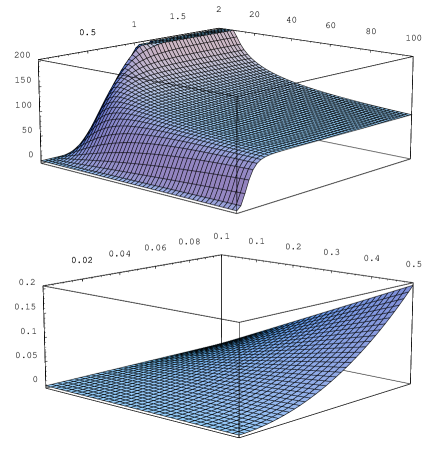
FIG. 2.: A plot of the Eq.(89): a) the general shape, b) a small $x$ behaviour.

It is interesting to note that $1/\pi^{2}\approx\pi^{2}/97$ which is almost the Stefan-Boltzmann constant. This once more vindicates our interpretation of $\sigma$ as a “temperature”. A plot of the pressure as a function of $\sigma$ is depicted in FIG.3. It is due to the low frequence modes contribution to the pressure that $P(\sigma)<P(T)$. This is a direct result of our choice of $g({\bf{k}})$, namely that $\sigma$ cannot be interpreted as temperature for the low frequence modes (i.e. $\omega_{k}<\sigma$). The smaller $\sigma$ is the less important contribution from non-equilibrium soft modes and so the smaller difference between both pressures.

The result (93) can be alternatively rewritten in terms of $\langle\beta\rangle$ . Using, for instance, the Padé approximation [31] for $\langle\beta\rangle$, we arrive at

$$P(\langle\beta\rangle) = 0.0681122\,{\langle\beta\rangle^{-4}}-0.0415368\,{\langle\beta\rangle^{-2}}{\cal M}^{2}$$ (94)

$$+ \lambda_{r}\,\left(-0.000647\,{\langle\beta\rangle^{-4}}+0.0000164\,{\langle\beta\rangle^{-2}}\,{\mathcal{M}}^{2}\right)$$ (95)

$$+ {\mathcal{O}}\left({\mathcal{M}}^{2}{\mbox{ln}}({\mathcal{M}}\langle\beta\rangle);\lambda_{r}^{2}\right).$$ (96)

The coefficient $0.0681122\approx\pi^{2}/145$ is $1.6$ times smaller than the required value for the Stefan-Boltzmann constant, so the parameter $\langle\beta\rangle$ is a slightly worse approximation of the equilibrium temperature than $\sigma$. In practice, however, it is a matter of taste and/or a particular context which of the above two descriptions is more useful.

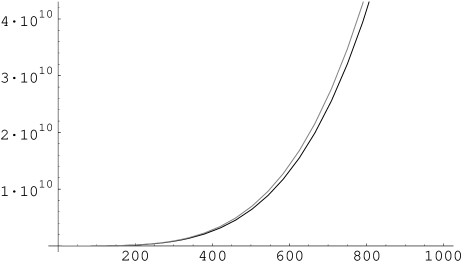
FIG. 3.: A plot of pressure as a function of $T$, $\sigma$ for $m_{r}=100\mbox{MeV}$. The gray line corresponds to equilibrium pressure, the black line corresponds to pressure (93).

FIG. 4.: A plot showing the difference of equilibrium and non-equilibrium pressures for $m_{r}=100\mbox{MeV}$.

C Off-equilibrium II

As was noted above, it is the specific form of the constraint $g({\bf{k}})$ which prescribes the behaviour of $\beta({\bf{k}})$. Let us now turn our attention to systems which depart ‘slightly’ from equilibrium, i.e. when $g({\bf{k}})$ in (59) deviates a little from the equilibrium density of energy per mode. In this case the constraint (59) reads

$$g({\bf{k}})=\frac{V}{(2\pi)^{3}}\,\frac{\omega_{k}}{e^{\beta_{0}\omega_{k}}-1}+\delta g({\bf{k}});\;\;\delta g({\bf{k}})\ll g({\bf{k}}),$$ (97)

with $\beta_{0}=1/T_{0}$ being an inverse of the equilibrium temperature. As a special example of (97) we choose

$$g({\bf{k}})=\frac{V}{(2\pi)^{3}}\,\frac{\omega_{k}}{e^{\beta_{0}\omega_{k}}\alpha^{-1}({\bf{k}})-1};\;\;\;\alpha({\bf{k}},\beta_{0})\approx 1.$$ (98)

The inverse mode “temperature” $\beta({\bf{k}})$ is then $\beta_{0}-\mbox{ln}(\alpha({\bf{k}}))/\omega_{k}$. So $\mbox{ln}(\alpha)$ measures (in units of $\omega_{k}$) the deviation of the mode temperature from the equilibrium one. The particular value of $\alpha({\bf{k}},\beta_{0})$ depends on the actual way in which the system is prepared. To avoid unnecessary technical complications, we select $\alpha({\bf{k}},\beta_{0})$ to be a momentum-space constant (generalisation is, however, straightforward). This choice represents the change in the mode temperature which is now inversely proportional to $\omega_{k}$; the deviation is bigger for soft modes and is rapidly suppressed for higher modes. Obviously, $T_{0}$ becomes the global temperature if $\omega_{k}\gg\mbox{ln}(\alpha)$. The generalised KMS conditions (63) together with solutions (66) determine $f_{++}$ as

$$f_{++}(k)={\alpha\over{e^{\beta_{0}\omega_{k}}-\alpha}}\,.$$ (99)

Eq.(99) is a reminiscent of the, so called, Jüttner distributionwith fugacity $\alpha$ [32, 33]. Now, using (49) and (77) we get for the pressure per particle

$$P+{\cal P}_{0} = {1\over 2\pi^{2}}\left[{{\cal M}^{2}\over\beta_{0}^{2}}\sum_{n=1}^{\infty}{\alpha^{n}\over n^{2}}K_{2}(n{\cal M}\beta_{0})\right.$$ (101)

$$+\left.{{\cal M}\delta m^{2}\over 4\beta_{0}}\sum_{n=1}^{\infty}{\alpha^{n}\over n}K_{1}(n{\cal M}\beta_{0})\right]\,,$$

where $\delta m^{2}$ satisfies the gap equation

$$\delta m^{2} = {\lambda_{r}\over 2}\left({\tilde{\Sigma}}(m^{2}_{r},\delta m^{2})+{1\over 2\pi^{2}}\int_{0}^{\infty}{k^{2}dk\over\omega_{k}}{\alpha\over{e^{\beta_{0}\omega_{k}}-\alpha}}\right)\,.$$ (102)

If we set, as before, $x=\delta m^{2}/m_{r}^{2}$ and $s=1/\beta_{0}m_{r}$ we get the transcendental equation for $x$

$$\lambda^{-1}_{r} = \frac{1}{32\pi^{2}x}\left\{(1+x)\mbox{ln}(1+x)-x\right.$$ (104)

$$+ \left.8(1+x)\;\int^{\infty}_{1}\,dz\,\sqrt{z^{2}-1}\,\frac{\alpha}{e^{z\,\sqrt{x+1}/s}-\alpha}\right\}.$$ (105)

The corresponding numerical analysis of (105) reveals that for $x\ll 1$ , $1/s\ll 1$. So at $x\ll 1$, $\lambda_{r}\approx\delta m^{2}/T_{0}^{2}$. This estimate is important for the asymptotic expansion of $\delta m^{2}$. However, in order to carry out the asymptotic expansion of (LABEL:precal5) (and consequently (101)) we need to cope first with the sum $\sum_{n=1}^{\infty}\alpha^{n}K_{k}(n{\cal M}\beta_{0})/n^{k}\,\,\,(k=1,2)$ (also called Braden’s function). Expansion of $K_{k}(\ldots)$ yields a double series which is very slowly convergent, and so it does not allow one to easily grasp the leading behaviour in $T_{0}$. In this case it is useful to resume (101)-(LABEL:precal5) by virtue of the Mellin summation technique [10]. (It is well known [10, 14, 34] that at equilibrium this resummation leads to a rapid convergence for high temperatures.) As a result, for a sufficiently large $T_{0}$ we get

$$\delta m^{2} = \frac{\lambda_{r}\,T^{2}_{0}}{24}-{\lambda_{r}T_{0}{\cal M}\over 4\pi}\left[{1\over 2}(1-r^{2})^{1/2}\right.$$ (106)

$$- \left.r\left(1-\ln\left({{\cal M}\over 2T_{0}}\right)\right)-(1-r^{2})^{1/2}\arcsin(r)\right]$$ (107)

$$+ {\cal O}(\ln T_{0})\;,$$ (108)

where we have set $r=\mbox{ln}(\alpha)T_{0}/{\cal M}$. The corresponding expansion of the pressure (101) reads

$$P = {\pi^{2}T_{0}^{4}\over 90}+{{\cal M}\zeta(3)\over\pi^{2}}T_{0}^{3}r-{T_{0}^{2}{\cal M}^{2}\over 24}\left(1-2r^{2}\right)-{{\cal M}^{3}T_{0}\over 4\pi^{2}}$$ (109)

$$\times \left[-{1\over 3}\left(1-r^{2}\right)^{\frac{3}{2}}+{r\over 2}\left(1-{2\over 3}r^{2}\right)\left(1-2\ln\left({{\cal M}\over 2T_{0}}\right)\right)\right.$$ (110)

$$- {2\over 9}\left(1-r^{2}\right)\bigg{(}-r^{3}+3-\left.3\left(1-r^{2}\right)^{\frac{1}{2}}\bigg{)}\arcsin(r)\right]$$ (111)

$$+ {(\delta m^{2})^{2}\over 2\lambda_{r}}+{\cal O}(\ln T_{0})\,.$$ (112)

where $\zeta(3)\approx 1.202$. Note that for $\alpha=1$ we regain the equilibrium expansion (57). The corresponding plot of $P$ as a function of $T_{0}$ and $\alpha$ is depicted in FIG.5.

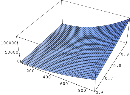
FIG. 5.: Behaviour of the pressure (101) as a function of $\alpha$ and $T_{0}$ at $m_{r}=100\mbox{MeV}$.

In passing it may be mentioned that the expansion (112) is mathematically justifiable only for $\alpha\approx e^{\sqrt{\lambda_{r}/24}\,r}\approx 1$.

VI Summary and Conclusions

In order to get a workable recipe for non-equilibrium pressure calculations we have combined three independent concepts: the Jaynes-Gibbs principle of maximal entropy, the Schwinger-Dyson equations, and the hydrostatic pressure. The basic steps are as follows.

To find quantitative results for pressure one needs to know the explicit form of the Green’s functions involved. These may be find if we solve the Dyson-Schwinger equations. The corresponding solutions are unique provided we specify the density matrix $\rho$ (the construction of $\rho$ is one of the cornerstones of our approach, and we tackled this problem using the Jaynes-Gibbs principle of maximal entropy). With $\rho$ at our disposal we showed how to formulate the generalised Kubo-Martin-Schwinger (KMS) boundary conditions.

To show how the outlined method works we have illustrated the whole procedure on an exactly solvable model, namely $O(N)\;\Phi^{4}$ theory in the large $N$ limit. This model is sufficiently simple yet complex enough to serve as an illustration of basic characteristics of the presented method in contrast to other ones in use. In order to find the constraint conditions we have considered two gedanken experiments in which the system in question was prepared in such a way that only low frequence modes departed from the strict equilibrium behaviour. Such processes can be found, for example, in ionised atmosphere, in laser stimulated plasma or in hot fusion [30]. In both alluded gedanken experiments we were able to work out the hydrostatic pressure exactly. Furthermore, after identifying a “temperature” parameter (virtually temperature of high modes) we carried out the corresponding high-temperature expansions.

As it was discussed, one of the main advantages of the Jaynes-Gibbs construction is that one starts with the (physical) constraints (i.e. parameters which are really controlled and measured in experiments). These constraints directly determine the density matrix and hence the generalised KMS conditions for the Dyson-Schwinger equations. This contrasts with the usual approaches where the density matrix is treated as the primary object. In these cases it is necessary to solve the von Neumann-Liouville equation. This is usually circumvent using either variational methods [24, 35] with several trial $\rho$’s or reformulating the problem in terms of the quantum transport equations for Wigner’s functions [36]. It is, however, well known that the inclusion of constraints into transport equations is a very delicate and rather complicated task (the same is basically true about the variational methods) [36, 37].

- [1]
- [2] T.D.Lee, in: Symmetries and fundamental interactions in nuclei, 1-13. eds. W.C.Haxton and E.M.Henley (Columbia University Press, 1997).
- [3] S.N.White, Nucl.Instrum.Methods A409 (1998) 618.
- [4] H.Heiselberg and A.D.Jackson, to be published in the proceedings of 3rd Workshop on Continuous Advances in QCD (QCD98), Minneapolis, MN, 16-19 Apr 1998.
- [5] R. Hagedorn, Z.Phys.C17 (1983) 265.
- [6] T.Haruyama, N.Kimura and T.Nakamoto, KEK-PREPRINT-98-113. C98-07-14. Aug 1998. 6pp. Presented at 17th International Conference on Cryogenic Engineering (ICEC 17), Bornemouth, England, 14-17 Jul 1998.
- [7] T.Haruyama, N.Kimura and T.Nakamoto, KEK-PREPRINT-97-156. C97-07-27.6. Sep 1997. 8pp. Talk given at Cryogenic Engineering Conference and International Cryogenic Materials Conference (CEC / ICMC 97), Portland, OR, 27 Jul - 1 Aug 1997.
- [8] S.Hull, D.A.Keen, R.Done and C.N.Uden, RAL-91-089. Dec 1991. 13pp.
- [9] J.Staun Olsen, L.Gerward and U.Benedict, DESY SR-84-22 (84,REC.OCT.) 19p.
- [10] N.P.Landsman and Ch.G.van Weert, Phys. Rep. 145, (1987) 141.
- [11] M.LeBellac, Thermal Field Theory (Cambridge University Press, Cambridge, 1996).
- [12] I.T.Drummond, R.R.Horgan, P.V.Landshoff and A.Rebhan, Phys.Lett. B398 (1997) 326.
- [13] G.Marc and W.G.McMillan, in: Advances in Chemical Physics, Vol. LVIII, eds. I.Prigogine and S.Rice (Wiley, New York, 1985).
- [14] P.Jizba, hep-th/9801197 (to appear in Phys.Rev.D).
- [15] E.Calzetta and B.L.Hu, Phys.Rev.D 37 (1988) 2878.
- [16] E.T.Jaynes, Phys.Rev 106 (1957) 620, 108 (1957) 171.
- [17] P.Jizba and E.S.Tututi, work in progress.
- [18] C.G.Callan, S.Coleman and R.Jackiw, Ann.Phys. 59 (1970) 42.
- [19] K.C.Chou, Z.B.Su, B.L.Hao and L.Yu, Phys. Rep. 118 (1985) 1.
- [20] J.Dougherty, Phil.Trans.R.Soc.Lond. A 346 (1994) 259.
- [21] L.E.Reichl, A Modern Course in Statistical Physics (Edward Arnold (Publishers), Ltd, 1987).
- [22] P.A.Henning, Nuclear Physics B337 (1990) 547.
- [23] L.P.Kadanoff and G.Baym, Quantum Statistical Mechanics (Benjamin, Reading, 1962).
- [24] O.Éboli, R.Jackiw and So-Young Pi, Phys.Rev.D 37 (1988) 3557.
- [25] F.Cooper and E.Mottola, Phys.Rev.D 36 (1987) 3114.
- [26] F.Cooper, S.Habib, Y.Kluger and E.Mottola, Phys.Rev.D 55 (1997) 6471.
- [27] J.Collins, Renormalization (Cambridge University Press, Cambridge, 1984)
- [28] L.S.Brown, Ann. Phys. (N.Y.) 126 (1980) 135.
- [29] G. Amelino-Camelia and S.-A. Pi, Phys.Rev. D47 (1993) 2356.
- [30] J.Dougherty, private communication.
- [31] G.A.Baker, Essentials of Padé Approximation (Academic Press, London, 1975).
- [32] R.Bair, M.Dirks, K.Redlich, and D.Schiff, Phys.Rev. D56 (1997) 2548.
- [33] M.Strickland, Phy.Lett. B331 (1994) 245.
- [34] H.E.Haber and H.A.Weldon, J.Math.Phys.23 (1982) 1852.
- [35] F.Floreanini and R.Jackiw, Phys. Rev.D 37 (1988) 2206.
- [36] R.Balescu, Equilibrium and Nonequilibrium Statistical Mechanics (John Wiley & Sons, London, 1975).
- [37] J.Baacke, K.Heitmann and C.Pätzold, hep-th/9711144.