HUTP-A072

hep-th/9810225

Thermodynamics of spinning D3-branes

Steven S. Gubser
Lyman Laboratory of Physics

Cambridge, MA 02138

Abstract

Spinning black three-branes in type IIB supergravity are thermodynamically stable up to a critical value of the angular momentum density. Inside the region of thermodynamic stability, the free energy from supergravity is roughly reproduced by a naive model based on free ${\cal N}=4$ super-Yang-Mills theory on the world-volume. The field theory model correctly predicts a limit on angular momentum density, but near this limit it does not reproduce the critical exponents one can compute from supergravity. Analogies with Bose condensation and modified matrix models are discussed, and a mean field theory improvement of the naive model is suggested which corrects the critical exponents.

October 1998

1 Introduction

Low-energy physics on the world-volume of $N$ coincident D3-branes [1] placed in flat ten-dimensional spacetime is dictated by ${\cal N}=4$ super-Yang-Mills theory (SYM) with gauge group $U(N)$ [2]. The gauge coupling and the closed string coupling are related by $g_{YM}^{2}=2\pi g_{s}$.

A cluster of coincident D3-branes can also be regarded as a black three-brane of ten-dimensional type IIB supergravity (SUGRA) [3]. The geometry has characteristic curvature scale $R=(4\pi g_{s}N\alpha^{\prime 2})^{1/4}$. Since the validity of supergravity depends on having curvatures small on both the string and Planck scales, both $N$ and $g_{YM}^{2}N$ must be large. Large ’t Hooft coupling, $\lambda=g_{YM}^{2}N\gg 1$, is the opposite limit to the one treatable in perturbation theory, so if supergravity does capture certain aspects of gauge theory, it is of strongly coupled gauge theory.

One of the earliest attempts to exploit the relation between supergravity and gauge theory as alternate low-energy descriptions of D3-branes was the computation of the entropy [4, 5]. The results disagree only by a numerical factor: in the microcanonical ensemble (which seems the most natural from the point of view of gravity),

$${s_{SUGRA}}$$

(1)

In (1), $s$ and $e$ are entropy and energy per unit world-volume. In supergravity, $s$ is computed using the Bekenstein-Hawking formula, and $e$ is computed as the ADM mass density above extremality. In super-Yang-Mills theory, $s$ and $e$ are computed using the free theory ($g_{YM}=0$). Conformal invariance dictates the $e^{3/4}$ behavior but not the coefficient. The disagreement in the coefficient is sometimes quoted as $4/3$ rather than $(4/3)^{1/4}$; this is the result of working in the canonical rather than the microcanonical ensemble. Given that the gravity and gauge theory calculations are valid in the limits of large and small ’t Hooft coupling, respectively, the puzzle is not so much that there is a numerical discrepancy in the coefficient but rather that the discrepancy is finite (that is, it does not depend parametrically on $N$ or the ’t Hooft coupling $\lambda$). It is as if the number of degrees of freedom in supergravity were exactly $3/4$ the number in the free theory. Indeed, it was pointed out in [4] that the discrepancy could be cured by excluding the gauge bosons and one species of gauginos from the free field counting. Because the gauginos transform in an irreducible representation of the R-symmetry group, this prescription breaks rotational invariance. A more likely scenario (recently challenged in [6]) is that the coefficient on the entropy interpolates smoothly between finite weak and strong coupling limits. It was shown in [7] that at least the leading $\alpha^{\prime}$ correction to supergravity perturbed the coefficient toward its free field theory value.

In section 2 we will extend the supergravity calculation to the case of the black three-brane with angular momentum in a plane perpendicular to the brane. The geometry was constructed explicitly in [8], following the work of [9]. This spinning three-brane has the same quantum numbers as $N$ coincident D3-branes with a density of $R$-charge on the world-volume equal to the angular momentum density $j$ (the $R$-symmetry group is precisely the rotation group $SO(6)$ in the dimensions transverse to the brane). Following the spirit of [4], we suggest that the supergravity geometry actually teaches us the strong-coupling thermodynamics of large-$N$ super-Yang-Mills theory. The salient feature of that thermodynamics is an instability for $j>N^{2}T^{3}$ (up to numerical factors of order unity).

It seems impossible to recover this prediction by a standard perturbative gauge theory calculation. Zero coupling is in a sense the worst place to be expanding around, because in the presence of charged massless bosons there cannot be any “voltage” for the charge density $j$. In section 4 we will suggest a formal approach for regulating the free field partition function in the presence of such a voltage. We do not claim that our approach invalidates the free field theory conclusion that massless bosons cannot support a chemical potential; however, it may be a better starting point from which to understand the strong coupling regime. In particular, we shall see that near $j=0$ the regulated free energy reproduces the supergravity results for thermodynamic quantities like specific heat and isothermal capacitance, up to factors of order unity. Furthermore, it also predicts thermodynamic instability for $j>N^{2}T^{3}$, again in agreement with supergravity up to a finite factor. The critical exponents are predicted incorrectly by the regulated field theory model, but we suggest that this might be fixed by a mean field treatment of interactions.

Our attention will be focused, both on the supergravity side and in the regulated field theory model, on the phase whose region of thermodynamic stability includes the states of small $T$ and zero $j$. We believe that the boundary of stability is actually a phase boundary beyond which another stable phase emerges. Our speculation is that in this phase the D3-branes spontaneously separate. The motivation for this guess will be explained at the end of the paper, but the bulk of it is devoted to three goals: 1) to demonstrate the existence of a boundary to the region of stability of the small $j$ phase; 2) to examine the critical properties of the thermodynamics near the boundary; and 3) to see how the thermodynamics might be reproduced in field theory.

2 Spinning three-brane thermodynamics

Since the rotation group $SO(6)$ transverse to a three-brane in ten dimensions has rank three, it is possible to give a three-brane three independent (commuting) angular momenta. We will use the solution constructed in [8], which has only one angular momentum, but there should be no difficulty in principle using the results of [9] to extend to the general case. The metric is

$${ds^{2}}$$

(2)

where

$${f}$$

(3)

and the dilaton is constant, as for the spherically symmetric case. Fixing the number $N$ of units of five-form flux leads to the constraint

$$r_{0}^{4}\sinh\alpha\cosh\alpha=R^{4}\equiv{N\kappa\over 2\pi^{5/2}}$$ (4)

where

$$2\kappa^{2}=16\pi G=(2\pi)^{7}g_{s}^{2}\alpha^{\prime 4}$$ (5)

is the gravitational constant of type IIB supergravity.

We define the energy of this solution as the ADM mass minus the mass of a supersymmetric, non-rotating three-brane with the same five-form flux: if $V$ is the spatial world-volume, then

$${e}$$

(6)

where we have used the BPS formula for the tension of the extremal three-brane, $M_{0}/V=N\sqrt{\pi}/\kappa$. The angular momentum conjugate to $\phi$ can be read off from the asymptotics of $g_{t\phi}$ [10]:

$$j={J^{xy}\over V}={\pi^{3}\over\kappa^{2}}\ell r_{0}^{4}\cosh\alpha\ .$$ (7)

Note that $e$ has dimensions of $(\hbox{length})^{-4}$ while $j$ has dimensions of $(\hbox{length})^{-3}$. Finally, the entropy

$$s={A_{H}/4G\over V}={2\pi^{4}\over\kappa^{2}}r_{H}r_{0}^{4}\cosh\alpha$$ (8)

is computed from the area $A_{H}$ of the event horizon, whose location $r_{H}$ is the unique real positive root of $\tilde{h}=0$: $r_{H}^{2}={\textstyle{1\over 2}}(\sqrt{\ell^{4}+4r_{0}^{4}}-\ell^{2})$ [8].

It is possible in principle to eliminate $\ell$, $r_{0}$, and $\alpha$ from (4), (6), (7), and (8), and express $s=s(e,j;N,R)$, where we regard $(e,j)$ as variables parameterizing the phase space and $N$ and $R=(4\pi g_{s}N\alpha^{\prime 2})^{1/4}$ as parameters specifying the theory. The nontrivial dependence on the dimensionful parameter $R$ makes it hopeless to try to reproduce this entropy function from ${\cal N}=4$ SYM, because ${\cal N}=4$ SYM is conformal: it has no scale. However, it was observed for $j=0$ already in [4] that the $R$-dependence drops out in the near-extremal limit $(M_{ADM}-M_{0})/M_{0}\ll 1$ (a startling consequence is that all dependence on the ’t Hooft parameter drops out as well, in the leading $\alpha^{\prime}$ approximation to type IIB string theory which type IIB supergravity represents). For $j=0$ one is left with an entropy function $s=s(e;N)$ which is unique up to an $N$-dependent normalization given conformal invariance of the underlying theory and extensivity of $S$ and $E$. For $j\neq 0$ the entropy function again becomes independent of $R$ in the near-extremal limit $r_{0},\ell\ll R$, but it involves a function of the dimensionless ratio $j^{4}/e^{3}$ that cannot be determined by scaling arguments. We will now determine it from supergravity.

The near-extremal limit has $\alpha\to\infty$, and $\alpha$ is conveniently eliminated in favor of $r_{0}$ using an approximation to (4), $e^{2\alpha}={2N\kappa\over\pi^{5/2}r_{0}^{4}}$. One immediately learns $e={\textstyle{3\over 2}}{\pi^{3}\over\kappa^{2}}r_{0}^{4}$, and with a bit more work $j=\ell\sqrt{\sqrt{\pi}Ne/3\kappa}$ and

$$s=s(e,j;N)={2^{5/4}3^{-3/4}\sqrt{\pi N}e^{3/4}\over\sqrt{\sqrt{1+\chi}+\sqrt{\chi}}}={\sqrt{2}\pi j\over\sqrt{\sqrt{\chi(1+\chi)}+\chi}}$$ (9)

where

$$\chi={27\pi^{2}\over 8N^{2}}{j^{4}\over e^{3}}\ .$$ (10)

The denominators represent the nontrivial new information we are gleaning from the spinning black hole solution.

As a safeguard against algebraic errors, and to check the normalization of (7), we have computed the angular velocity $\Omega$ at the horizon. $\Omega$ is defined by requiring the Killing vector $\partial/\partial t+\Omega\,\partial/\partial\phi$ to be null at the horizon. One finds

$$\Omega={\ell r_{H}^{2}\over r_{0}^{4}\cosh\alpha}\to\pi\sqrt{6}{j\over N\sqrt{e}}\left(\sqrt{1+\chi}-\sqrt{\chi}\right)\ .$$ (11)

The first expression for $\Omega$ is exact; the second represents the near-extremal limit. In this limit, one can check from (9) that

$$\Omega=-{(\partial s/\partial j)_{e}\over(\partial s/\partial e)_{j}}\ ,$$ (12)

as required by the first law of black hole thermodynamics: $dE=TdS+\Omega dJ$.

3 The limits of thermodynamic stability

Our primary interest in this section is the thermodynamic stability of near-extremal spinning D3-branes. As a warmup, let us study the stability of non-rotating black 3-branes which are not required to be near-extremal. The entropy function $s=s(e;N,R)$ has a rather complicated form when written out explicitly. It is simpler to refrain from eliminating the variable $\alpha$ from (6) and (8), since then we have

$${e}$$

(13)

In this simple example, thermodynamic stability is equivalent to positivity of the specific heat at constant volume, $C_{V}=(\partial E/\partial T)_{V}$. In manipulations of thermodynamic quantities, we will always hold $V$ fixed, and we will usually drop the subscript $V$ that indicates this explicitly. Also we will work with intensive quantities only. Inspection of (13) reveals that while $e$ is strictly decreasing with $\alpha$, $T$ has a quadratic maximum at $\alpha=\alpha_{c}$ where $\mathop{\rm coth}\nolimits^{2}\alpha_{c}=3$. This indicates a singularity, $c_{V}\sim 1/\sqrt{T-T_{c}}$, in the specific heat, since

$$c_{V}={\partial e\over\partial T}={\partial e/\partial\alpha\over\partial T/\partial\alpha}\ ,$$ (14)

and $T\sim T_{c}-(\alpha-\alpha_{c})^{2}$ near the critical point. For $\alpha<\alpha_{c}$, $c_{V}<0$, so this region is unstable. Note that the scale of the phase transition is set by $R$, so it can’t have anything to do with renormalizable ${\cal N}=4$ super-Yang-Mills theory. If it has any world-volume interpretation, it seems it would have to be in terms of an effective, possibly non-local theory like the Born-Infeld generalization of electromagnetism. On the supergravity side, the phase transition is much less arcane: it is the standard transition from positive to negative specific heat that occurs as mass is added to almost any charged black hole solution. The thermodynamic instability is real in the sense that Schwarzschild black holes really do get colder when you increase their mass.

What we will find for the near-extremal limit of spinning D3-branes is a boundary of thermodynamic stability with the same $1/\sqrt{T-T_{c}}$ singularity in a specific heat, but with the critical temperature $T_{c}$ set by the angular momentum density rather than a scale built into the theory. In other words, it is an effect which falls inside the putative regime of validity of the renormalizable super-Yang-Mills theory description of the world-volume. Spinning three-branes with $T<T_{c}$ are unstable, and the question we begin to address next is how one might see this boundary of stability in field theory.

It is slightly more subtle to evaluate thermodynamic stability when the entropy function $S=S(x_{1},\ldots,x_{n})$ depends non-trivially on several extensive thermodynamic variables $x_{i}$. The criterion is sub-additivity:

$$S(\{\lambda x_{i}+(1-\lambda)\tilde{x}_{i}\})\geq\lambda S(\{x_{i}\})+(1-\lambda)S(\{\tilde{x}_{i}\})$$ (15)

for $\lambda$ between $0$ and $1$. When $S(\{x_{i}\})$ is a smooth function, one can simply demand that the Hessian matrix $\left[\partial^{2}S/\partial x_{i}\partial x_{j}\right]$ has no positive eigenvalues.

Applying the above considerations to the entropy function (9), we see that the condition for thermodynamic stability is $\chi\leq 1/3$. Equivalently, we may demand that the energy function

$$e(s,j)={\textstyle{3\over 2}}{s^{4/3}\over N^{2/3}(2\pi)^{2/3}}\left(1+{4\pi^{2}j^{2}\over s^{2}}\right)^{1/3}$$ (16)

derived from (9) has a positive definite Hessian. This also leads to $\chi\leq 1/3$, or more usefully

$${j\over s}\leq{1\over\sqrt{2}\pi}\ .$$ (17)

Since the Hessian matrix $\left[\partial^{2}e/\partial x_{i}\partial x_{j}\right]$ can also be written as $\left[\partial y_{i}/\partial x_{j}\right]$ where $y_{i}=\partial e/\partial x_{i}$, a positive definite Hessian means that the functions $y_{i}=y_{i}(x_{1},\ldots,x_{n})$ are invertible—ie that we can Legendre transform freely among the various ensembles.

The ensemble which will be most directly comparable to the naive field theory model developed in section 4 is the one where $(s,j)$ are both traded for their dual variables $(T,\Omega)$. We will call this the grand canonical ensemble because it is like having indefinite particle number and a chemical potential. The free energy in this ensemble is usually called the grand potential, and we will denote it as $\Xi$. It is related to $E$ by

$$E=\Xi+TS+J\Omega\ .$$ (18)

Written as a function $\Xi(T,\Omega,V)$ of the volume plus the intensive quantities temperature and voltage, the grand potential is forced by extensivity to be linear in $V$. Indeed, $-\xi=-\Xi/V=P$ is just the pressure. Conformal invariance implies $\xi=-{\textstyle{1\over 3}}e$. In deriving the explicit expression

$${\xi(T,\Omega)}$$

(19)

the following “equation of state” is useful:

$${\Omega\over T}={2\pi^{2}j/s\over 1+2\pi^{2}j^{2}/s^{2}}\ .$$ (20)

The region of allowed $\Omega/T$ is restricted:

$${\Omega\over T}\leq{\pi\over\sqrt{2}}\ ,$$ (21)

which as the reader can check expresses the maximum value the right hand side of (20) can attain as a function of $j/s$. The boundary of stability (17) occurs at the maximum value of $\Omega/T$, so the (21) is not a good description of the boundary of stability: the equality is obtained at the boundary, but on both sides $\Omega/T$ decreases. It is possible to quote the stability condition in the canonical ensemble, where $T$ and $j$ are fixed: the condition is

$$j={9\pi\over 16\sqrt{2}}N^{2}T^{3}\ .$$ (22)

There is really only one critical exponent in the description of the thermodynamics near the boundary of stability. It characterizes the approach of $\xi$ to its value at criticality: at fixed temperature,

$$\xi=\xi_{c}+j_{c}(\Omega_{c}-\Omega)-A(\Omega_{c}-\Omega)^{2-\gamma}+O\left[(\Omega_{c}-\Omega)^{2}\right]\ .$$ (23)

where $A$ is some constant and, for the case at hand, $\gamma=1/2$. All other critical exponents follow from this one using scaling properties. In particular, the specific heat $c_{\Omega}$ at constant voltage goes as $(T-T_{c})^{-\gamma}$. With $\gamma=1/2$, this is the same $1/\sqrt{T-T_{c}}$ behavior we saw in the non-rotating example at the beginning of this section.

4 A naive field theory model

Let us first recall the spectrum of ${\cal N}=4$ super-Yang-Mills theory. Besides the gauge bosons, which have no charge under the $R$ symmetry group $SO(6)\approx SU(4)$, there is a (color) adjoint of Weyl fermions $\lambda^{a}$ in the ${\bf 4}$ of $SU(4)$ and an adjoint of scalars $X^{i}$ in the ${\bf 6}$ of $SO(6)$. Under the subgroup $SO(2)$ of $SO(6)$ generated by $\partial/\partial\phi$, half of the fermions (that is, $4N^{2}$ degrees of freedom) have charge $1/2$ and the other half have charge $-1/2$, whereas of the scalars, two thirds ($4N^{2}$ degrees of freedom) are neutral, one sixth have charge $1$, and the last sixth have charge $-1$ (note that we have included particles and anti-particles explicitly in our counting). All these particles are massless since we have not Higgsed the theory.

The presence of charged massless bosons makes it impossible to apply a “voltage” $\Omega$ of the $SO(2)$ subgroup to the free theory, simply because one of the thermal occupation factors $n_{\pm}(\vec{p})=1/(e^{\beta(|\vec{p}|\pm\Omega)}-1)$ will become negative for $|\vec{p}|<|\Omega|$. The interactions, treated perturbatively in the ’t Hooft coupling $\lambda$, result in a thermal mass $m\sim\sqrt{\lambda}T$ to lowest order. Thus it seems the critical value of the potential $\Omega$ is $\Omega_{c}=\sqrt{\lambda}T$ up to a factor of order unity: parametrically different from the supergravity result. Factors of $\lambda$ will also enter into thermodynamic quantities like isothermal capacitance $(\partial j/\partial\Omega)_{T}$ measured at $j=\Omega=0$. There is nothing contradictory in supposing that in fact $\Omega_{c}=f(\lambda)T$ for some function $f(\lambda)$ which approaches a constant for $\lambda\to\infty$ and $\sqrt{\lambda}$ for $\lambda\to 0$; and likewise for the various measurable quantities like $(\partial j/\partial\Omega)_{T}\Big{|}_{\Omega=0}$.

Positing an interpolating function for every quantity that disagrees between free field theory and supergravity may be in some sense the correct thing to do, but it is highly non-predictive, particularly since both the perturbation expansion in finite temperature field theory and the $\alpha^{\prime}$ expansion in string theory are difficult to compute past the first nontrivial term. In hopes of establishing a better field theory understanding of the supergravity results, we will suggest in section 4.1 a method of regularizing the free field theory partition function so that it becomes well-defined at finite voltage. In section 4.2 we will see that this naive field theory treatment has some degree of success in reproducing the phenomena observed in supergravity. In section 4.3 we will try to improve the naive model using mean field theory.

4.1 A regulation scheme

In this section we will suggest a regulation of integrals over $n_{\pm}(\vec{p})$ which makes predictions for the critical voltage $\Omega_{c}$ and for $(\partial j/\partial\Omega)_{T}\Big{|}_{\Omega=0}$ which agree up to factors of order unity with the supergravity results. It is not our aim to revise free field theory; rather, we hope that our procedure captures in some sense a better approximation to the dynamics of the effective excitations of interacting super-Yang-Mills theory. The factor of $N^{2}$ on the grand potential $\xi$ in (19) is an indication that there are $N^{2}$ degrees of freedom excited at finite temperature, even in the limit of strong coupling. We regard this as a clue that perhaps some adaptation of the free theory can be used to approximate the statistical mechanics of the interacting one.

The divergent integrals that occur in free field theory with a chemical potential for massless bosons are of the form

$$\int_{0}^{\infty}dp\,{p^{n-1}\over e^{p-\mu}-1}=\Gamma(n)\sum_{j=1}^{\infty}{(e^{\mu})^{j}\over j^{n}}=\Gamma(n)\mathop{\rm Li}\nolimits_{n}(e^{\mu})$$ (24)

$$\int_{0}^{\infty}dp\,p^{n-1}\log(1-e^{\mu-p})=-\Gamma(n)\mathop{\rm Li}\nolimits_{n+1}(e^{\mu})\ .$$ (25)

where $\mathop{\rm Li}\nolimits_{n}$ is the polylogarithm function, which is defined by the sum in (24) when its argument is in the unit disk. This function can be analytically continued to the complex $\mu$-plane, and it is analytic except for a branch cut along the positive real axis. The imaginary part changes sign across this cut while the real part is continuous. The principle value prescription for the integrals in (24) and (25) for real $\mu$ is to average the values for $\mu+i\epsilon$ and $\mu-i\epsilon$. This amounts to replacing $\mathop{\rm Li}\nolimits_{n}$ by its real part $\Re\mathop{\rm Li}\nolimits_{n}$. One might be inclined to regard the principle value prescription as a species of infrared regulation, similar in spirit to differential regulation in its use of analytic continuation to define divergent integrals. But it differs from the use of an explicit mass as a regulator in that it yields a cutoff-independent free energy which is stable in a finite region including zero voltage. We will show that if both regularizations are applied at once, then by making the explicit mass small one smoothly recovers the massless case.

Using this prescription on (24) one can calculate the charge density $j$ for a given potential $\Omega$ by integrating the thermal occupation factors. We will instead use (25) to compute the grand potential density $\xi=\Xi/V=\xi(T,\Omega;N)$, from which all other thermodynamic quantities follow by differentiation. For a collection of several species of free massless charged particles in a potential $\Omega$,

$$\xi=T\int{d^{3}p\over(2\pi)^{3}}\sum_{i}s_{i}\log(1-s_{i}e^{-\beta(|\vec{p}|-q_{i}\Omega)})=-{T^{4}\over\pi^{2}}\sum_{i}s_{i}\mathop{\rm Li}\nolimits_{4}(s_{i}e^{\beta q_{i}\Omega})\ .$$ (26)

The sum over $i$ is over particle species. For each species, $q$ is the charge and $s=1$ or $-1$ according as the particle is a boson or a fermion. For fermions, the principle value prescription is superfluous because the polylogarithm is evaluated at negative argument and so is already real. For free ${\cal N}=4$ $U(N)$ SYM, (26) specializes to

$${\xi}$$

(27)

where we have used the identity (valid for positive integers $n$)

$$\mathop{\rm Li}\nolimits_{n}(e^{\mu})+(-1)^{n}\mathop{\rm Li}\nolimits_{n}(e^{-\mu})=\sum_{j=0}^{\lfloor n/2\rfloor}{2\zeta(2j)\over(n-2j)!}\mu^{n-2j}\pm{i\pi\over(n-1)!}\mu^{n-1}\ .$$ (28)

The explicit sign on the imaginary term in (28) is the same as the sign of the imaginary part of $\mu$. From (27) one can extract the charge density:

$$j=-\left({\partial\xi\over\partial\Omega}\right)_{T}={\textstyle{1\over 2}}N^{2}T^{3}\left[{\Omega\over T}-{1\over 4\pi^{2}}{\Omega^{3}\over T^{3}}\right]\ .$$ (29)

As an aside, it is interesting to note that the two terms in (27) pertaining to the charged scalars individually have singularities in their second derivatives at the origin, but their sum is $C^{\infty}$. If we were to change the charge of the scalar or give it a mass without making the corresponding change to its anti-particle required by CPT, this singularity would reappear. In a non-relativistic system of massive particles (that is, the usual Bose-Einstein setup),

$${j}$$

(30)

where we have again applied the principle value prescription to the integral for $\mu>0$. $\partial j/\partial\mu$ is singular at the origin and negative for $\mu>0$, indicating thermodynamic instability. Thus in the case of non-relativistic bosons, one recovers through the principle value prescription the standard conclusion that the disordered phase in a free Bose gas is stable only up to a charge density $j=\zeta(3/2)(mT/2\pi)^{3/2}$.

Let us now consider the case of a relativistic massive boson:

$$j=\int{d^{3}p\over(2\pi)^{3}}\left({1\over e^{\beta(\sqrt{p^{2}+m^{2}}-\Phi)}-1}-{1\over e^{\beta(\sqrt{p^{2}+m^{2}}+\Phi)}-1}\right)\ ,$$ (31)

where we have included the anti-particle in the second term. We will regard the mass as an explicit infrared regulator of the massless theory. The integral is not one of the standard special functions. However, its singularity structure as a function of the complex parameter $\Phi$ is easy to determine: it is analytic except for branch cuts on the real axis for $|\Phi|>m$. The branch cuts are discontinuities of the imaginary part. If one applies the principle value prescription for real $\Phi$, one gets a continuous function $j(\Phi)$ which is smooth except for a “kink” at $|\Phi|=m$, where the function itself remains finite but its first derivative is singular. In standard free field theory, this kink is the signal for Bose condensation. But if we continue past this kink using the principle value prescription, and if $m$ is not too large, we find a new region where $\partial j/\partial\mu>0$. The size of the kink scales as $(m/T)^{3/2}$. In the $m\to 0$ limit, it disappears altogether and we recover a cubic curve qualitatively identical to (29) (it differs in exact coefficients because (29) includes the effects of fermions). The convergence of $j(\Phi;m)$ to $j(\Phi;0)$ as $m\to 0$ is uniform. If the principle value prescription is used uniformly, physical quantities defined in a theory with an explicit mass as the infrared cutoff have a smooth behavior as that infrared cutoff is removed. Note however that the cubic curve (29) shows no sign of Bose condensation at $\Phi\to 0$. Its thermodynamic stability will be the subject of section 4.2.

4.2 Thermodynamics of the naive field theory model

The reader who is distrustful of the regulation methods used in the section 4.1 may at least be willing to regard

$$\xi=-{\pi^{2}\over 8}N^{2}T^{4}\left[{4\over 3}+{2\over\pi^{2}}{\Omega^{2}\over T^{2}}-{1\over 4\pi^{4}}{\Omega^{4}\over T^{4}}\right]$$ (32)

as a motivated guess for the field theory partition function. But is it a good guess? In this section we will show that (32) exhibits a boundary of stability at a value of ${j\over N^{2}T^{3}}$ differing from the supergravity result (22) only by a finite factor, but that the critical exponent $\gamma$ is different. In section 4.3 we will argue that the correct critical exponent can be obtained through a mean field theory improvement of (32).

The agreement up to factors of order unity of the first two terms in square brackets in (32) with the corresponding terms in (19) implies a similar agreement in the small $\Omega$ limit of all thermodynamic quantities expressible in terms of second derivatives of the various free energies: such quantities can be related to entries in the Hessian matrix of $\xi(T,\Omega)$, which is

$$\pmatrix{{\partial^{2}\xi\over\partial T^{2}}&{\partial^{2}\xi\over\partial T\partial\Omega}\cr\vskip 3.0pt\cr{\partial^{2}\xi\over\partial\Omega\partial T}&{\partial^{2}\xi\over\partial\Omega^{2}}}=\left\{\vbox{\openup 3.0pt\halign{\strut\hfil$\displaystyle{#}$& $\displaystyle{{}#}$\hfil\cr&-{\textstyle{3\over 2}}N^{2}\pi^{2}T^{2}\pmatrix{1&{\Omega\over 3\pi^{2}T}\cr\vskip 3.0pt\cr{\Omega\over 3\pi^{2}T}&{1\over 6\pi^{2}}}\left(1+O[\Omega^{2}/T^{2}]\right)\quad\hbox{for SUGRA}\cr\vskip 9.0pt\cr&-{\textstyle{3\over 2}}N^{2}\pi^{2}T^{2}\pmatrix{{4\over 3}&{2\Omega\over 3\pi^{2}T}\cr\vskip 3.0pt\cr{2\Omega\over 3\pi^{2}T}&{1\over 3\pi^{2}}}\left(1+O[\Omega^{2}/T^{2}]\right)\quad\hbox{for field theory.}\cr}}\right.$$ (33)

The upper left entry reflects the well-known $4/3$ disagreement of the non-rotating case. The $\Omega^{4}/T^{4}$ term in square brackets in (19) and (27) are of opposite sign, and so also some of the $O[\Omega^{2}/T^{2}]$ terms which we have not indicated explicitly in (33) disagree in sign between supergravity and field theory. This is in fact the first symptom of the disagreement in critical exponents at the boundary of stability.

It is already a nontrivial fact, however, that the regulated field theory predicts a boundary of stability at finite $\Omega/T$. Let us see how it arises. Thermodynamic stability requires that the Hessian matrix of $\xi(T,\Omega)$ be negative definite. This is so when

$${\Omega\over T}\leq 2\pi\sqrt{{2\over\sqrt{3}}-1}\ .$$ (34)

Note that this is a smaller value than the one we might guess by analogy with Bose condensation from the behavior of $j(T,\Omega)$: the maximum of $j(T,\Omega)$ for positive $\Omega$ and fixed $T$ is attained at $\Omega/T=2\pi/\sqrt{3}$, which is greater than the right hand side of (34). It is more enlightening to examine the “equation of state”

$${j\over s}={3\over 4\pi^{2}}{\Omega\over T}{1-{1\over 4\pi^{2}}{\Omega^{2}\over T^{2}}\over 1+{3\over 4\pi^{2}}{\Omega^{2}\over T^{2}}}\ .$$ (35)

Here the maximum of the right hand side does occur precisely at the boundary of stability.

By expanding $\xi$ in (27) at fixed $T$ around the critical value of $\Omega$, one finds the behavior (23) with $\gamma=0$. No derivatives of $\xi$ become singular: for example, at fixed temperature, $c_{\Omega}\sim(\Omega_{c}-\Omega)^{-\gamma}=const$. As one can see from figure 1, $c_{\Omega}$ smoothly approaches a maximum as $\Omega\to\Omega_{c}$.

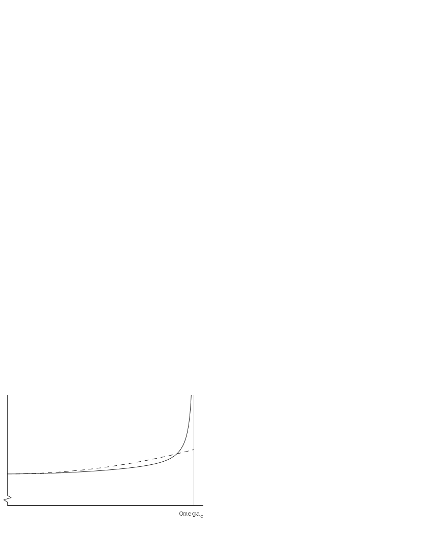
Figure 1: $c_{\Omega}$ as a function of $\Omega$ for fixed $T$, in supergravity (solid line) and in the naive field theory model (dashed line). The horizontal and vertical axes have been scaled differently for the two curves so that the boundary of stability occurs at the same point $\Omega_{c}$, and so that the two curves meet at $\Omega=0$.

4.3 Interactions and modified critical behavior

The comparison between supergravity and the naive field theory model is a little like the comparison between superfluidity in ${}^{4}{\rm He}$ and Bose condensation in an ideal gas [11, 12]. The free field treatment of Bose condensation predicts the location of the ${}^{4}{\rm He}$ phase transition to within $30\%$. But whereas in the free field treatment the specific heat has a finite peak at the transition temperature, in real ${}^{4}{\rm He}$ it exhibits a $\log(T-T_{c})$ divergence. The interactions modify the critical behavior.

There is also an example of logarithmic corrections to critical scaling in an exactly soluble model of two-dimensional quantum gravity: the modified matrix models [13, 14, 15, 16, 17]. In matrix models one typically has an expansion

$${\cal F}\sim\hbox{(analytic in $\Delta$)}+\Delta^{2-\gamma}+\hbox{(higher order in $\Delta$)}\ .$$ (36)

for the free energy. Here $\Delta$ is the cosmological constant, which is taken to zero to obtain large random surfaces, and $\gamma$ is termed the string susceptibility. The standard $c=1$ model has $\Delta^{2}/\log\Delta$ as the leading nonanalytic term. One can introduce a $(\mathop{\rm tr}\nolimits\Phi^{2})^{2}$ term, which can be regarded as an interaction among otherwise free fermions in a potential well. The positions of the fermions are the eigenvalues of the matrix $\Phi$. If the strength of the interaction is tuned appropriately, it alters the critical behavior of $c=1$ to $\Delta^{2}\log\Delta$ (and, incidentally, changes the location of the critical point in the coupling space of the matrix model by a finite factor). This is like going from $\gamma$ barely negative to $\gamma$ barely positive. For $c<1$, the shift is finite, and again changes the sign of $\gamma$: upon adding the interaction, $\gamma\to\bar{\gamma}=\gamma/(\gamma-1)$.

It is our hope that by including an effective description of the interactions in our field theory model, we may see a similar modification in the critical behavior—optimistically, one which will predict $\gamma=1/2$.

Let us try to evaluate whether this is a realistic hope by considering a mean field theory treatment. One can suppose that the presence of a density $j$ of $R$-charge sets up a “self-field” contribution to the voltage. In order to work in terms of dimensionless quantities (as conformal invariance demands), we assume a relation

$${\Omega_{\rm tot}\over T}={\Omega\over T}+f\left({j\over N^{2}T^{3}}\right)$$ (37)

where $f(\rho)$ is some function to be determined. We obtain a consistency condition by replacing $j$ in (37) with the integral over thermal occupation factors:

$$j\to\int{d^{3}p\over(2\pi)^{3}}\sum_{i}q_{i}{1\over e^{\beta(|\vec{p}|-q_{i}\Omega_{\rm tot})}-s_{i}}$$ (38)

where as before $i$ indexes particles, $q_{i}$ is the charge, and $s_{i}=1$ for bosons and $-1$ for fermions. The integral is regulated using the principle value prescription. (38) boils down to replacing $\Omega$ by $\Omega_{\rm tot}$ in (29) and then plugging the resulting expression for $j$ back into (37). Note however that the physical charge density must be obtained by differentiating the grand potential $\xi$ by the applied voltage $\Omega$. The grand potential is obtained by replacing $\Omega$ by $\Omega_{\rm tot}$ in (27). Using the consistency condition one can write $\xi$ wholly in terms of $\Omega$ and $T$.

To shorten the formulas, let us introduce some notation for dimensionless quantities:

$${j\over N^{2}T^{3}}=\rho\qquad{\Omega\over T}=\omega\qquad{\Omega_{\rm tot}\over T}=\omega_{\rm tot}\ .$$ (39)

Then the grand potential can be written as

$$-{\xi\over N^{2}T^{4}}\equiv\tilde{g}(\omega)=g(\omega_{\rm tot})\equiv{\pi^{2}\over 6}+{\textstyle{1\over 4}}\omega_{\rm tot}^{2}-{1\over 32\pi^{2}}\omega_{\rm tot}^{4}\ ,$$ (40)

and the consistency condition is

$$\omega=\omega_{\rm tot}-f(g^{\prime}(\omega_{\rm tot}))=\omega_{\rm tot}-f\left({\textstyle{1\over 2}}\omega_{\rm tot}-{1\over 8\pi^{2}}\omega_{\rm tot}^{3}\right)\ .$$ (41)

Primes will always denote the differentiation of a function with respect to its argument.

The quantity $\mu=\partial\omega_{\rm tot}/\partial\omega$ can be regarded in analogy with $\partial B/\partial H$ in magnetic systems as a permeability: $\mu>1$ is the analog of paramagnetism, where the self-field contribution reinforces the applied voltage, and $\mu<1$ is the analog of diamagnetism. Let $\mu_{0}$ be the permeability at zero voltage. Modulo a constraint on the behavior of $f(\rho)$ for finite $\rho$, we claim that $\gamma=1/2$ arises precisely when $\mu_{0}=2/3$, and otherwise $\gamma=0$ or $3/2$ according as $\mu_{0}>2/3$ or $\mu_{0}<2/3$. The constraint is that $f(\rho)$ must be such that

$$4\tilde{g}(\omega)\tilde{g}^{\prime\prime}(\omega)-3\tilde{g}^{\prime}(\omega)^{2}>0$$ (42)

for $\omega$ less than the value where $\omega_{\rm tot}=\omega_{{\rm tot},c}\equiv 2\pi$. This is a special point because $g^{\prime}(2\pi)=0$. We will refer to (42) as the convexity constraint because it is precisely the requirement that the Hessian matrix of $\xi(T,\Omega)$ be negative definite.

First note by explicit differentiation of (41) that $\mu_{0}=2/3$ is equivalent to $f^{\prime}(0)=-1$. Let us assume $\mu_{0}=2/3$. Then $\partial\omega/\partial\omega_{\rm tot}=0$ at $\omega_{\rm tot}=\omega_{{\rm tot},c}$. Near $\omega_{\rm tot}=\omega_{{\rm tot},c}$ we have

$${\omega_{c}-\omega}$$

(43)

Plugging the first equation into the second, one obtains

$$\tilde{g}(\omega)=\tilde{g}_{0}+\tilde{g}_{1}(\omega_{c}-\omega)+\tilde{g}_{3/2}(\omega_{c}-\omega)^{3/2}+O[(\omega_{c}-\omega)^{2}]$$ (44)

which indicates that indeed $\gamma=1/2$. The reader interested in the details will have no trouble verifying

$${\omega_{c}} {{}=\omega_{{\rm tot},c}=2\pi} {a_{2}} {{}={3\over 4\pi}} {a_{3}} {{}={\textstyle{1\over 6}}f^{\prime\prime\prime}(0)-{1\over 8\pi^{2}}} {g_{0}} {{}={2\pi^{2}\over 3}} {g_{2}} {{}=-{\textstyle{1\over 2}}} {g_{3}} {{}={1\over 4\pi}} {\tilde{g}_{0}} {{}={2\pi^{2}\over 3}} {\tilde{g}_{1}} {{}=-{2\pi\over 3}} {\tilde{g}_{3/2}} {{}={4\over 27}\sqrt{\pi\over 3}(3+2\pi^{2}f^{\prime\prime\prime}(0))\ .}$$ (45)

In (45) we have used the fact that $f(-\rho)=-f(\rho)$ by symmetry, so all even derivatives of $f(\rho)$ vanish at the origin. The critical charge density is given by

$${j\over N^{2}T^{3}}=\rho_{c}=-\tilde{g}_{1}={2\pi\over 3}\ .$$ (46)

For $\mu_{0}<2/3$, $\partial\omega/\partial\omega_{\rm tot}<0$ at $\omega_{\rm tot}=\omega_{{\rm tot},c}$. This makes it impossible to invert (41) to obtain $\omega_{\rm tot}$ as a single-valued function of $\omega$ past the maximum value for $\omega$, which is obtained at some value $\omega_{\rm tot}=\omega_{{\rm tot},m}<\omega_{{\rm tot},c}$. Because $g^{\prime}(\omega_{{\rm tot},m})\neq 0$, this scenario leads to $\gamma=3/2$. For $\mu_{0}>2/3$, $\omega_{{\rm tot},c}$ could still be the critical point if (42) is not violated earlier, but there would be a linear term in $\omega_{{\rm tot},c}-\omega_{\rm tot}$ in the expression for $\omega_{c}-\omega$ in (43), so $\tilde{g}(\omega)$ would be analytic in $\omega$ near $\omega_{c}$: $\gamma=0$, as we saw with no interactions included at all. So only at the special value $\mu_{0}=2/3$ can we see the $\gamma=1/2$ behavior predicted by supergravity. The precise shape of $\tilde{g}(\omega)$ depends on the behavior of $f(\rho)$ for finite $\rho$. But the location $\omega_{c}=2\pi$ of the boundary of stability and the prediction $\gamma=1/2$ rely only on $f^{\prime}(0)=-1$—again, modulo the convexity requirement (42). It may be entertaining for the reader to note that with $\mu_{0}=2/3$ the discrepancy between the isothermal capacitance in field theory and supergravity is a factor of $8/9$, which is numerically an improvement over the factor of $2$ that we saw for $\mu_{0}=1$ in (33).

At this point we must ask if it is indeed possible to satisfy (42) for $0<\omega_{\rm tot}<2\pi$, because if (42) is violated for $\omega_{\rm tot}<\omega_{{\rm tot},c}=2\pi$, then the system becomes thermodynamically unstable “by accident” before one can come to the special point $\omega_{\rm tot}=\omega_{{\rm tot},c}$, and all our analysis will have been for nothing. As long as $\omega$ is a strictly increasing function of $\omega_{\rm tot}$, (42) is equivalent to requiring that

$${\partial\over\partial\omega_{\rm tot}}\left[{1\over g(\omega_{\rm tot})}\left({\partial g/\partial\omega_{\rm tot}\over\partial\omega/\partial\omega_{\rm tot}}\right)\right]>0\ ,$$ (47)

so a necessary condition (and also a sufficient one if $\partial\omega/\partial\omega_{\rm tot}>0$ can be shown) is to require (47) for $0<\omega_{\rm tot}<2\pi$. We do not have complete results on what restrictions this implies on the behavior of $f(\rho)$. However, it is straightforward to verify that linear functions $f(\rho)=2{\mu_{0}-1\over\mu_{0}}\rho$ satisfy the requirement if and only if $\mu_{0}=2/3$. For $\mu_{0}<2/3$, linear $f(\rho)$ results in $\gamma=3/2$ in the way described in the previous paragraph. For $\mu_{0}>2/3$, in fact the critical point occurs for $\omega_{\rm tot}<\omega_{{\rm tot},c}=2\pi$, and $\gamma=0$ by an analysis qualitatively identical to the case with no interactions at all.

It is conceivable that through some peculiar singular behavior of $f(\rho)$ at finite $\rho$ one could arrange $\gamma=1/2$ and a smaller critical value for $\omega_{\rm tot}$. Of course, such a setup would seem extremely ad hoc unless one had a justification for the particular form of $f(\rho)$ from an analysis of the interactions. Such an analysis is highly desirable at this point, at least for small $\rho$. It would be particularly amusing if the strong coupling limit $\lambda\to\infty$ managed somehow to tune $\mu_{0}$ to $2/3$. Indirect evidence for whether this is happening might be extracted from a study of $\alpha^{\prime}$ corrections in the supergravity, along the lines of [7].

5 Conclusions

We have investigated the thermodynamics of coincident D3-branes spinning in a plane orthogonal to the branes. Using the standard techniques of black hole thermodynamics we obtained an expression for the entropy which indicates thermodynamic stability only up to a special value of the dimensionless ratio of the angular momentum density and the temperature. We can write all thermodynamic functions in terms of intensive quantities because conformal invariance forbids the presence of any dimensionful parameters: any function of dimensionful variables can be re-expressed in terms of intensive quantities by scaling each variable by the appropriate power of the volume. The absence of a scale means that physical relations like an equation of state or the location of a boundary of stability must be expressible in terms of dimensionless ratios of intensive quantities. It also implies that only one critical exponent, $\gamma$, describes the approach of the world-volume theory to the boundary of stability. It for instance gives the scaling law $c_{\Omega}\sim(T-T_{c})^{-\gamma}$ at fixed voltage (as explained above, voltage $\Omega$ is the thermodynamic variable dual to $R$-charge). We have found $\gamma=1/2$ from supergravity.

In the superconformal field theory which characterizes low-energy fluctuations of the branes, angular momentum is interpreted as electric charge under a subgroup of the $R$-symmetry group. We have suggested an alteration of free field theory in which one can calculate very simply the critical value of the angular momentum density where the phase transition takes place. The calculation employs the thermodynamic ensemble where voltage rather than $R$-charge density is held fixed. This ensemble is formally ill-defined when there are free massless charged bosons. The alteration of free field theory which we have suggested relies on a regulation procedure employing analytic continuation to render all the relevant integrals finite. The reader is entitled to question the validity of our regulation scheme: negative thermal occupation number is a serious pathology. Nevertheless, if supergravity is supposed to be teaching us about super-Yang-Mills theory at strong coupling, then spinning black holes show that the theory is stable up to voltages on the order of the temperature. A description of the interacting theory has to start somewhere, and our starting point, the regulated free field theory, enjoys a measure of success. It leads to an expression for the grand potential which exhibits a boundary of stability similar to the one observed in supergravity, and at a similar value of the charge density at fixed temperature.

The regulated field theory wrongly predicts $\gamma=0$. In analogy to Bose condensation and the modified matrix models, we have suggested that including an effective description of the interactions may change the scaling behavior. We have substantiated this claim by showing in mean field theory that if the three-branes respond “diamagnetically” to an applied voltage (that is, if the total voltage on the branes is reduced from the applied voltage by a self-field contribution) then the scaling behavior can be modified to $\gamma=1/2$. One obtains $\gamma=1/2$ at a special value, $\mu_{0}=2/3$, of the “permeability.” This value separates a region of $\gamma=0$ behavior ($\mu_{0}>2/3$) from a region of $\gamma=3/2$ behavior ($\mu_{0}<2/3$). The regulated free field theory and the mean field treatment of interactions are not motivated by any deep understanding of strong coupling gauge dynamics, but rather by a desire to see in a simple way how and whether finite-temperature field theory can reproduce the thermodynamics of spinning near-extremal D3-branes.

The analysis of this paper leaves us at a point similar to the state of matrix models of two-dimensional quantum gravity: we have a description of critical behavior near a boundary, but on the other side of the boundary our description breaks down. In the matrix models, the intuition was that eigenvalues were leaking out of the local potential well and falling down a $V(\lambda)\sim-\lambda^{4}$ hill. A clear description of the physics seemed difficult because it demanded a “non-perturbative” definition of two-dimensional quantum gravity. In Bose condensation a new stable phase (the Bose condensate) emerges on the other side of the boundary. The obvious analog of Bose condensation on D3-branes is Higgsing: some of the scalars develop expectation values. This suggests that the cluster of coincident branes should be splitting up, perhaps into a ring (condensed state) around a central core (normal state). A supergravity solution of this type may be difficult to write down explicitly. If it could be shown that there is a correlation length in the scalar fields on the uncondensed side of the phase transition which diverges at the boundary, we would regard it as evidence in favor of the Higgsing scenario. We hope to report on these issues in the future.

Note Added

After this work was completed, we received the paper [18] which has a tangential relation to section 2 of this paper. In [18] the Euclidean version of the spinning three-brane solution was considered. The thermodynamics is qualitatively different because the angular momentum and velocity are imaginary. The entropy function that follows from (3.24) of [18] can be obtained formally from our results by replacing $\sqrt{\chi}\to-\sqrt{\chi}$ in the first expression for $s$ in (9).

References

- [1] J. Polchinski, “Dirichlet branes and Ramond-Ramond charges,” Phys. Rev. Lett. 75 (1995) 4724–4727, hep-th/9510017.
- [2] E. Witten, “Bound states of strings and p-branes,” Nucl. Phys. B460 (1996) 335–350, hep-th/9510135.
- [3] G. T. Horowitz and A. Strominger, “Black strings and p-branes,” Nucl. Phys. B360 (1991) 197–209.
- [4] S. S. Gubser, I. R. Klebanov, and A. W. Peet, “Entropy and temperature of black 3-branes,” Phys. Rev. D54 (1996) 3915–3919, hep-th/9602135.
- [5] A. Strominger, unpublished.
- [6] M. Li, “Evidence for large N phase transition in N=4 super-Yang-Mills theory at finite temperature,” hep-th/9807196.
- [7] S. S. Gubser, I. R. Klebanov, and A. A. Tseytlin, “Coupling constant dependence in the thermodynamics of N=4 supersymmetric Yang-Mills theory,” hep-th/9805156.
- [8] J. G. Russo, “New compactifications of supergravities and large N QCD,” hep-th/9808117.
- [9] M. Cvetic and D. Youm, “Rotating intersecting M-branes,” Nucl. Phys. B499 (1997) 253, hep-th/9612229.
- [10] R. C. Myers and M. J. Perry, “Black holes in higher dimensional space-times,” Ann. Phys. 172 (1986) 304.
- [11] F. London, Superfluids. Wiley, New York, 1954.
- [12] J. Wilks, The Properties of Liquid and Solid Helium. Oxford University Press, Oxford, 1967.
- [13] S. R. Das, A. Dhar, A. M. Sengupta, and S. R. Wadia, “New critical behavior in d = 0 large N matrix models,” Mod. Phys. Lett. A5 (1990) 1041–1056.
- [14] F. Sugino and O. Tsuchiya, “Critical behavior in c = 1 matrix model with branching interactions,” Mod. Phys. Lett. A9 (1994) 3149–3162, hep-th/9403089.
- [15] S. S. Gubser and I. R. Klebanov, “A modified c = 1 matrix model with new critical behavior,” Phys. Lett. B340 (1994) 35–42, hep-th/9407014.
- [16] I. R. Klebanov, “Touching random surfaces and Liouville gravity,” Phys. Rev. D51 (1995) 1836–1841, hep-th/9407167.
- [17] I. R. Klebanov and A. Hashimoto, “Nonperturbative solution of matrix models modified by trace squared terms,” Nucl. Phys. B434 (1995) 264–282, hep-th/9409064.
- [18] C. Csaki, Y. Oz, J. Russo, and J. Terning, “Large N QCD from rotating branes,” hep-th/9810186.