EFI-98-53

hep-th/9810224

Black Holes and the SYM Phase Diagram. II

Emil Martinec   and    Vatche Sahakian

Enrico Fermi Inst. and Dept. of Physics

University of Chicago

5640 S. Ellis Ave., Chicago, IL 60637, USA

The complete phase diagram of objects in M-theory compactified on tori $T^{p}$, $p=1,2,3$, is elaborated. Phase transitions occur when the object localizes on cycle(s) (the Gregory-Laflamme transition), or when the area of the localized part of the horizon becomes one in string units (the Horowitz-Polchinski correspondence point). The low-energy, near-horizon geometry that governs a given phase can match onto a variety of asymptotic regimes. The analysis makes it clear that the matrix conjecture is a special case of the Maldacena conjecture.

1 Introduction and summary

The Matrix and Maldacena conjectures [1, 2, 3] boldly propose a great simplification of the dynamics of M-theory in certain limits. Both postulate that all of M-theory – restricted to a sector of particular boundary conditions – is equivalent to super Yang-Mills theory (SYM). Conversely, we learn that nonperturbative super Yang-Mills is of a complexity equivalent to M-theory. Taking both conjectures into account, we expect that maximally supersymmetric Yang-Mills on $T^{p}$, $p\leq 3$, has dynamics of perturbative gauge theory, of near-horizon D-brane geometry, and of light-cone (LC) M-theory, all as different regimes in some grand phase diagram.

The aim of this paper is to map out the thermodynamic phase diagram of this theory. The finite temperature vacuum will acquire various geometrical realizations, and a rich thermodynamical structure will emerge. One conclusion is that, taking as inputs the Maldacena conjecture and the various duality symmetries of M-theory established at the level of the low energy dynamics, the Matrix conjecture is a necessary output. The point is that one can glue a given near-horizon structure onto several descriptions of the asymptotic region at large distance from the object. The choice of asymptotic description fixes a duality frame, and hence the physical interpretation of the parameters. Nevertheless, one can have e.g. a near-extremal D3-brane in type IIB theory whose thermodynamics is described by the 11D Schwarzschild black hole geometry. Which is the appropriate low-energy geometry to describe the horizon physics is governed by the proper size of the torus near the horizon, which depends on the horizon radius or entropy of the object. Qualitatively, at high entropy the Dp brane perspective is appropriate, as the horizon torus is large; at low entropies, the horizon torus is small, and a T-dualized D0 brane description is appropriate. This is the T-duality used in Matrix theory. To avoid cumbersome changes of notation, we will phrase the discussion in the language of light cone M-theory, even when the entropy is large enough that a dual D-brane description is appropriate; we hope this does not cause undue confusion.

The statement of the Maldacena conjecture identifies a dual geometrical structure with the (possibly finite temperature) vacuum of a SYM Quantum Field Theory (QFT). Physics of elementary excitations off this vacuum are mapped onto the physics of elementary probes in the background of the near-horizon geometries of branes [4, 5]. A non-trivial UV-IR correspondence relates radial extent in the bulk geometry and energy scale of such excitations [6, 7]. On the other hand, equilibrium thermodynamic states of SYM excitations get associated to geometries with thermodynamic character, i.e. supergravity vacua with finite area horizons. The UV-IR correspondence then amounts to essentially the holographic relation between area in the bulk and entropy in the SYM. Alternatively, it relates temperature in a QFT to radial extent in a non-extremal bulk [7].

When studying the thermodynamics of M-theory via that of a SYM, we then encounter on the phase diagram patches with dual supergravity realizations. Geometrical considerations will identify stability domains, transition curves and various equations of state. The global structure of the diagram should reflect the myriad of duality symmetries that M-theory is endowed with; geometry will paint the global structure of M-theory’s finite temperature vacuum. The basic idea then becomes a systematic analysis of various supergravity solutions; the underlying strategy goes as follows: A $10$D or lower-dimensional near-extremal supergravity solution must satisfy the following restrictions:

• The dilaton at the horizon must be small. Otherwise, in a IIA theory, we need to lift to an $11$D M-theory; in a IIB theory, we need to go to the S-dual geometry. This amounts to a change of description – a reshuffling of the dominant degrees of freedom – without any change in the equation of state.

• The curvature at the horizon must be smaller than the string scale. Otherwise, the dynamics of massive string modes becomes relevant. By the Horowitz-Polchinski correspondence principle [8], a string theory description emerges – an excited string, or a perturbative SYM gas reflecting weakly coupled D-brane dynamics. This is generally associated with a change of the equation of state; in the thermodynamic limit, we may expect critical behavior associated with a phase transition. This criterion can easily be estimated for various cases when one realizes that the curvature scale is set by the horizon area divided by cycle sizes measured at the horizon; i.e. the localized horizon area should be greater than order one in string units.

• Cycles of tori on which the geometry may be wrapped, as measured at the horizon, must be greater than the string scale [9]. Otherwise, light winding modes become relevant and the T-dual vacuum describes the proper physics [10]. We expect no critical behavior in the thermodynamic limit, since the duality is merely a change of description.

• The horizon size of the geometry must be smaller than the torus cycles as measured at the horizon [11, 12]. Otherwise, the vacuum smeared on the cycles is entropically favored. We expect this to be associated with a phase transition, one due to finite size effects, and it is associated generally with a change of the equation of state. However, it is also possible that there is no such entropically favored transition by virtue of the symmetry structure of a particular smeared geometry, so we expect no change of phase. Intuitively, a system would only localize itself in a more symmetrical solution to minimize free energy.

On the other hand, given an $11$D supergravity vacuum, a somewhat different set of restrictions applies:

• The curvature near the horizon must be smaller than the Planck scale. By the criterion outlined above, we see that, for unsmeared geometries, this is simply the statement that $S>1$; i.e. quantum gravity effects are relevant for low entropies. For large enough longitudinal momentum $N$, this region of the phase diagram is well away from the region of interest.

• The size of cycles of the torus as measured at the horizon must be greater than the Planck scale. Otherwise, we need to go to the IIA solution descending from dimensional reduction on a small cycle. We expect no change of equation of state or critical behavior.

• The size of the M-theory cycles, including the light cone longitudinal box, as measured at the horizon, must be bigger than the horizon size. Otherwise, the geometry gets smeared along the small cycles. This is expected to be a phase transition due to finite size physics.

Applying these criteria, we then select the near extremal geometry dual to a SYM theory on the torus, and navigate the phase diagram via duality transformations suggested by the various restrictions. We will then be mapping out the phase diagram of M-theory, or alternatively SYM QFT; we now present the results of such an analysis.

Figure (1) depicts the thermodynamic phase diagram of light cone M-theory

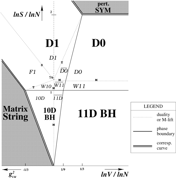
Figure 1: Phase diagram of Light Cone M theory on $T^{1}$; $S$ is entropy, $V$ is the radius of the circle in Planck units, $N$ is the longitudinal momentum. The geometry label dictionary is as follows: D0: black D0; $\overline{D0}$: black D0 smeared on $V$; D1: black D1; F1: black IIB string; W10: black IIA wave; W11: $11$D black wave; $\overline{W11}$: $11$D black wave smeared on $V$; $10$D BH: IIA LC black hole; $11$D BH: LC M-theory black hole; $\overline{11D}$ BH: LC M-theory BH smeared on $V$. $M$, $T$ and $S$ stand for respectively an M-duality (such as reduction, lift or M flip on $T^{3}$), a T-duality curve, and an S duality transition.

on the circle; the axes are entropy $S$, and the radius of the circle measured in Planck units $V$; $N$, the longitudinal momentum charge, is fixed. In general, the effective SYM coupling and torus radii are

$$\Sigma=\frac{{\it l}_{{\rm pl}}^{2}}{R_{11}V}\quad,\qquad g_{\rm eff}^{2}\sim g_{Y}^{2}NT^{p-3}\sim V^{-p}N\left(\frac{T{\it l}_{{\rm pl}}^{2}}{R_{11}}\right)^{p-3}$$ (1)

($T\sim E/S$ is the temperature). On the diagram, the behavior of the effective SYM coupling depends on the equation of state governing a given region under consideration. For $p<4$, the effective coupling increases as we move vertically downward in the D0 phase, and diagonally toward the bottom-left in the Dp brane phase. The raw Yang-Mills coupling (measured at the scale of the torus) increases horizontally as we move toward smaller M theory volumes $V^{p}$ for all $p$. The unshaded areas are described by various supergravity solutions, while the shaded regions do not have dual geometrical descriptions. On the upper right, there is a perturbative $1+1$D SYM gas phase living on the circle; and a Matrix string phase in the IR of the SYM, characterized by the emergence of $Z_{N}$ order, on the left at strong coupling. Dotted lines denote various duality transformations on the supergravity solutions; the equation of state is unchanged upon crossing such a line, since duality is merely a change of description. The solid lines denote localization transitions; double solid lines are curves associated with the principle of correspondence of Horowitz-Polchinski. These lines demarcate phase boundaries, where the equation of state changes. In total, we have six different thermodynamic phases. We observe the emergence of a self-duality point at $S\sim N^{7/6}$, $V\sim 1$. That the various patches do not overlap is a self-consistency check on the logical structure of the picture. For high entropies, localization effects are circumvented; the phases are the ones studied in [13]. The triple point on the upper right corner was the one studied in [9]. The lower left triple point was the one studied in [14]. This picture patches together these previous results on one diagram, in addition to identifying one additional triple point and the self-duality point. The oblique correspondence curve in the upper right corner can easily be seen to correspond to the point where the effective dimensionless Yang-Mills coupling is of order one. More interesting is the horizontal correspondence curve along $S\sim N^{2}$ starting at $V\sim N^{1/3}$. From the perturbative SYM side, it is where the thermal wavelength becomes of order the size of the box dual to $V$; from the D0 phase side, it is a Horowitz-Polchinski correspondence curve. As we will see below, the temperature jumps discontinuously as function of the entropy across this line. In [9], a separate phase consisting of a gas of super Quantum Mechanics excitations was identified with this curve when the phase diagram is plotted on the temperature-’t Hooft coupling plane. This transition may be associated with rich microscopic physics. From the thermodynamic perspective, as the transition is crossed, dynamics is transferred from local excitations in $p$+1 SYM to that of its zero modes; and Dp brane charge of the perturbative SYM is traded for longitudinal momentum charge of light cone M-theory. This process is one of several paths on the phase diagram relating the Maldacena and Matrix conjectures .

Figures (2) and (3) depict the phase diagrams of

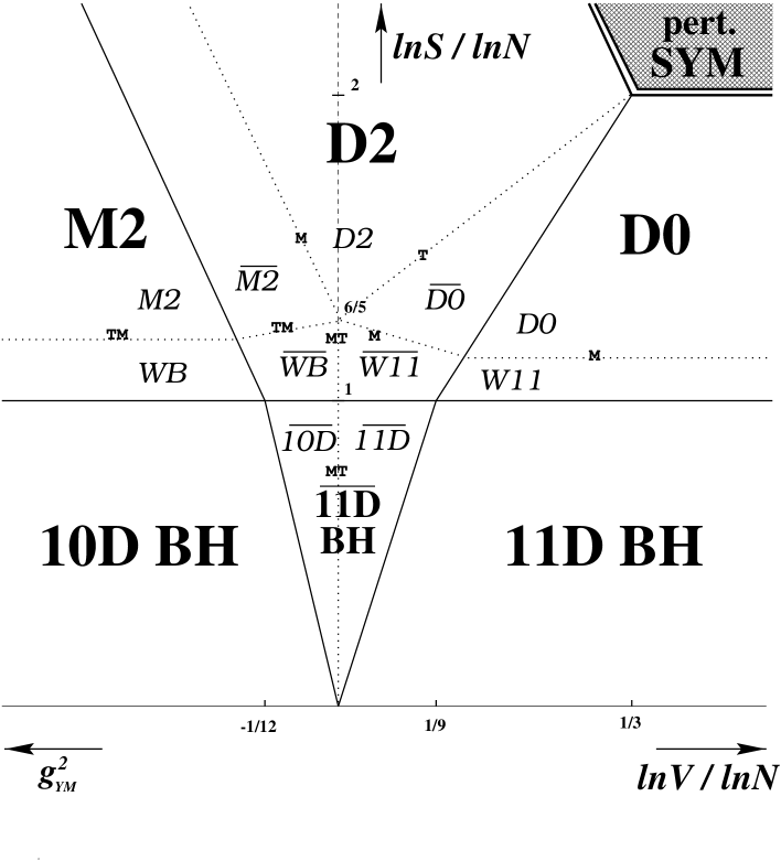
Figure 2: Phase diagram of Light Cone M theory on $T^{2}$; $V$ is the radius of the circle in Planck units. The geometry label dictionary is as follows: D0: black D0; $\overline{D0}$: black D0 smeared on $V$; D2: black D2; M2: black membrane; $\overline{M2}$: black membrane smeared on a dual circle; WB: black IIB wave; $\overline{WB}$: black IIB wave smeared on a dual circle; W11: $11$D black wave; $\overline{W11}$: $11$D black wave smeared on $V$; $11$D BH: light cone M-theory black hole; $\overline{11D}$ BH: light cone M-theory black hole smeared on $V$; $10$D BH: IIB light cone black hole; $\overline{10D}$ BH: IIB light cone black hole smeared on a dual circle.

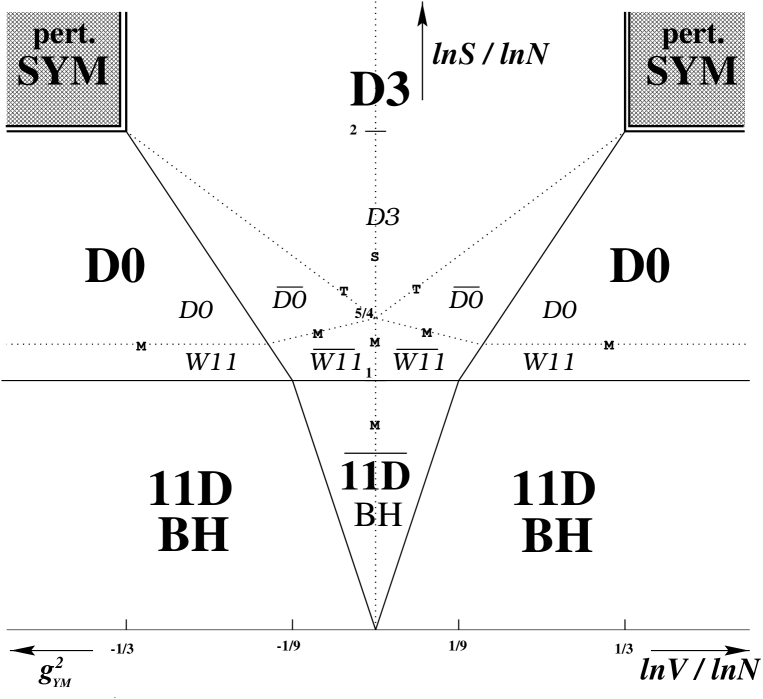
Figure 3: Phase diagram of Light Cone M theory on $T^{3}$. D0: black D0; $\overline{D0}$: black D0 smeared on $V$; D3: black D3; W11: $11$D black wave; $\overline{W11}$: $11$D black wave smeared on $V$; $11$D BH: light cone M-theory black hole; $\overline{11D}$ BH: light cone M-theory black hole smeared on $V$.

light cone M-theory on $T^{2}$ and $T^{3}$; $V$ here is the radius of the cycles (which are chosen to be equal) measured in Planck units. We have similar observations to the ones made for the previous $1+1$D SYM case. In the strong coupling region of SYM on $T^{2}$, the SYM dynamics approaches the infrared fixed point governing the dynamics of M2 branes – the conformal field theory dual to M-theory on $AdS_{4}\times S^{7}$ (in ‘Poincare’ coordinates). The proper size of the $T^{2}$ shrinks toward the origin; at high entropy, the black M2 geometry accurately describes the low-energy physics, while at low entropy the near-horizon geometry is best described in terms of the IIB theory dual to M-theory on $T^{2}$ [18]. In the $T^{3}$ case, the diagram reflects the self-duality of the D3 branes and M-theory on $T^{3}$ as reflection symmetry about $V\sim 1$. The ’t Hooft scaling limit focusses in on the neighborhood of the vertical line at $ln\,V/ln\,N\rightarrow\pm\frac{1}{3}$ (see equation (1)). The structure of all three of these phase diagrams can be checked by minimizing the Gibbs energies between the various phases identified.

Finally, we conclude with the following observation. Starting with a thermodynamic phase in light cone M-theory, say for example the lower right corner phase of the $11$D boosted black hole, using geometrical considerations, the duality symmetries of M-theory, and the Horowitz-Polchinski correspondence with the perturbative SYM phase, we would be led to conclude that light cone M-theory thermodynamics is encoded in the thermodynamics of SYM QFT. Indeed, the Maldacena conjecture asserts that underlying all these phases is super Yang-Mills theory in various regimes of its parameter space. Having not known the Matrix conjecture, we would then have been led to it from Maldacena’s proposal. The Matrix conjecture is a special realization of the more general statement of Maldacena. Correspondingly, our ability to discover the low-energy theories that yield matrix theory on some background depends on our ability to understand duality structures with less supersymmetry in sufficient detail to construct the phase diagram analogous to figures 1-3.

This introduction and summary set forth all our qualitative results and conclusions. The computational details can be found in the next section.

2 The details

The theory is parametrized by the Planck scale ${\it l}_{{\rm pl}}$, longitudinal radius $R_{11}$, and $p$ circle radii $R$. We define $V\equiv R/{\it l}_{{\rm pl}}$. The Maldacena or Matrix limit is

$${\it l}_{{\rm pl}}\rightarrow 0\mbox{ , with }{\it l}_{{\rm pl}}^{2}/R_{11}\mbox{ and }{\it l}_{{\rm pl}}/R\mbox{ fixed.}$$ (2)

We will begin by treating various geometries for $1\leq p\leq 3$ collectively, with $p$ a variable; we will then have to analyze separately regions of the phase diagram where significant differences arise between the different cases.

2.1 Stretched and smeared geometries

We first study the phases where the horizon is stretched or smeared along compact directions. The former case corresponds to situations where an extended object is wrapped on compact directions; the geometry cannot localize on such cycles by virtue of the symmetry structure of the metric. The latter case corresponds to solutions which are smeared along cycles because they would otherwise not ‘fit in the box’; these are prone to localization transitions to more symmetric, entropically favored horizon geometries. Both cases are endowed with the isometries of translation along the cycles. The solutions are parametrized by two harmonic functions

$$h=1-\left(\frac{r_{0}}{r}\right)^{7-p}\ ,$$ (3)

$$H=1+\left(\frac{q}{r}\right)^{7-p}\ .$$ (4)

From the area-entropy relation of the corresponding geometries, we have

$$r_{0}^{9-p}\sim\left(S^{2}/N\right){\it l}_{{\rm pl}}^{9-p}V^{-p}\ ,$$ (5)

while Gauss’s law yields

$$q^{7-p}\sim\frac{{\it l}_{{\rm pl}}^{9-p}}{R_{11}^{2}}\frac{N}{V^{p}}\ .$$ (6)

This last statement is valid for $q\gg r_{0}$, which is the case in the limit (2) with $S$, $N$ and $V$ finite. For large $N$, when interested in the thermodynamic limit of a large number of degrees of freedom, this limit is certainly satisfied.

We will track the full form of the geometries; at the end of the day, the conjecture requires us to look at the near horizon region, $q\gg r$.

Dp brane phase: This phase is described by the equation of state of black Dp branes

$$E\sim\frac{R_{11}}{{\it l}_{{\rm pl}}^{2}}\left(\frac{S^{2}}{N}\right)^{\frac{7-p}{9-p}}V^{2\frac{p}{9-p}}\ ,$$ (7)

and comprises of the geometries of stretched black Dp branes, smeared D0 branes, and smeared $11$D black waves. We now analyze each in turn.

The black Dp brane (D1,D2,D3) is given by the solution [19]

$$ds^{2}=H^{-1/2}\left(-hdt^{2}+d{\vec{y}}_{p}^{2}\right)+H^{1/2}\left(h^{-1}dr^{2}+r^{2}d\Omega_{8-p}^{2}\right)\ ,$$ (8)

$$e^{\phi}=g_{\it str}H^{(3-p)/4}\ ,$$ (9)

$$F_{rty}=g_{\it str}^{-1}\partial_{r}H^{-1}\ .$$ (10)

The theory is parametrized by

$$\alpha^{\prime}=\frac{{\it l}_{{\rm pl}}^{3}}{R_{11}}\quad,\qquad g_{\it str}=\left(\frac{R_{11}}{{\it l}_{{\rm pl}}}\right)^{(3-p)/2}V^{-p}\ ,$$ (11)

and the coordinates $\vec{y}$ are compactified on circles of size ${\it l}_{{\rm pl}}^{2}V^{-1}/R_{11}$. The relevant restrictions are:

• Small coupling at the horizon requires

  $$\left(N^{8-p}S^{p-7}\right)^{3-p}V^{3p(p-7)}<1\ .$$ (12)

  Otherwise, for $p=1,3$, we have to go to the S-dual geometry of black IIB fundamental strings or black D3 branes respectively; for $p=2$, we need to analyze smeared black M2 branes.

• Curvature at the horizon smaller than the string scale requires

  $$N^{6-p}V^{-3p}>S^{3-p}\ .$$ (13)

  Otherwise, we invoke the principle of correspondence – a perturbative $p+1$D SYM phase emerges.

• Requiring the cycle size of the $y$’s at the horizon to be greater than the string scale yields

  $$S>N^{\frac{8-p}{7-p}}V^{3\frac{6-p}{7-p}}\ .$$ (14)

  Otherwise, we go to the T-dual geometry of smeared D0 branes.

The smeared D0 brane ($\overline{D0}$) is the T-dual of (8) on the torus $T^{p}$ of the $y_{i}$

$$ds^{2}=-H^{-1/2}hdt^{2}+H^{1/2}\left(dy_{p}^{2}+h^{-1}dr^{2}+r^{2}d\Omega_{8-p}^{2}\right)\ ,$$ (15)

$$e^{\phi}=g_{\it str}H^{3/4}\ ,$$ (16)

$$A_{t}=g_{\it str}^{-1}\left(H^{-1}-1\right)\ .$$ (17)

The theory is parametrized by

$$\alpha^{\prime}=\frac{{\it l}_{{\rm pl}}^{3}}{R_{11}}\quad,\qquad g_{\it str}=\left(\frac{R_{11}}{{\it l}_{{\rm pl}}}\right)^{3/2}\ ,$$ (18)

and the new coordinates $\vec{y}$ are compactified on the scale ${\it l}_{{\rm pl}}V$. The restrictions are:

• Small coupling at the horizon requires

  $$S>N^{\frac{8-p}{7-p}}V^{\frac{p}{p-7}}\ .$$ (19)

  Otherwise, we have to lift to an $11$D M theory black wave solution.

• The correspondence point is (13).

• Requiring the ‘box’ size of the $y_{i}$ at the horizon to be smaller than the object yields

  $$S>V^{9/2}N^{1/2}\ ,$$ (20)

  independent of $p$. Otherwise, the system collapses into a localized D0 geometry along the torus $T^{p}$ parametrized by the $y_{i}$.

The smeared $11$D black wave ($\overline{W11}$) is the M-lift of (15)

$$ds^{2}=\left(H-1\right)\left(dx_{11}-dt\right)^{2}+dx_{11}^{2}-dt^{2}+H^{-1}\left(1-h\right)dt^{2}+dy_{p}^{2}+h^{-1}dr^{2}+r^{2}d\Omega_{8-p}^{2}\ ,$$ (21)

The theory is parametrized by the light cone M theory Planck scale ${\it l}_{{\rm pl}}$, the coordinates $\vec{y}$ are compactified on ${\it l}_{{\rm pl}}V$ as before, while $x_{11}$ lives on $R_{11}$. The new constraints are:

• Requiring the size of $x_{11}$ measured at the horizon to be greater than the Planck scale leads to the reverse of (19), patching back to the smeared D0 geometry.

• The size of the $y$ cycles measured at the horizon must be greater than the Planck scale

  $$V>1\ .$$ (22)

  Otherwise, we have to dimensionally reduce on a $y$ to a IIA geometry. For $p=1$, this will be a IIA black wave. For $p=2$, the new geometry will have cycles smaller than the string scale; so, we need to go to the T-dual vacuum representing a IIB black wave; this is of course just the well known duality between M theory on a shrinking $T^{2}$ and IIB on the circle. For $p=3$, we emerge into a dual M-theory with a black wave geometry.

• Requiring the ‘box’ size associated with $x_{11}$ measured at the horizon to be smaller than the object yields

  $$S>N\ .$$ (23)

  Otherwise, the system collapses into an $11$D black hole smeared along $\vec{y}$.

• Requiring the ‘box’ size associated with the $y_{i}$ measured at the horizon to be smaller than the object yields (20); the new geometry would be an $11$D black wave localized on the $y_{i}$.

Smeared $11$D black hole ($\overline{11D}$ BH): This is the Schwarzschild black hole in light cone M-theory on $T^{p}$ with Planck scale ${\it l}_{{\rm pl}}$, and torus radii $R_{11}$ and $R$, such that the solution is smeared on $T^{p}$. The form of the metric will be discussed later. The equation of state is given by

$$E\sim\left(\frac{R_{11}}{N}\frac{1}{{\it l}_{{\rm pl}}^{2}}\right)V^{2\frac{p}{9-p}}S^{2\frac{8-p}{9-p}}\ .$$ (24)

• The correspondence principle yields

  $$S>V^{p}\ ,$$ (25)

  which will always be satisfied. Particularly, for $p=0$, we have the statement $S>1$. At large $N$, this very low entropy regime passes out of the region of interest.

• For $V<1$, we reduce to a IIA geometry; for $p=1$, this is a IIA hole; for $p=2$, we need to go to the T-dual IIB hole solution for reasons discussed above; for $p=3$, we have a smeared $11$D hole in the dual M theory on $T^{3}$.

• Finally, the localization transition can be found by equating (24) to the energy of the $p=0$ phase, yielding

  $$S\sim V^{9}\ .$$ (26)

2.2 Localized geometries

The localized solutions are obtained from the above geometries (15) and (21) when the box size associated with the $y_{i}$ measured at the horizon becomes greater than the size of the object. The system collapses then into a more symmetric, entropically favored solution by the substitution

$$d{\vec{y}}_{p}^{2}+h^{-1}dr^{2}+r^{2}d\Omega_{8-p}^{2}\rightarrow h^{-1}dr^{2}+r^{2}d\Omega_{8}\ .$$ (27)

The entropy-area relationship changes to

$$r_{0}\sim{\it l}_{{\rm pl}}S^{2/9}N^{-1/9}\ ,$$ (28)

and the functions $H$ and $h$ become

$$h\rightarrow 1-\left(\frac{r_{0}}{r}\right)^{7}\ ,$$ (29)

$$H\rightarrow 1+c\left(\frac{{\it l}_{{\rm pl}}^{9}}{R_{11}^{2}}N\right)\frac{1}{r^{7}}\ .$$ (30)

Here $c$ is some numerical constant.

In the subsequent subsections, parameters and solutions can be obtained from their smeared relatives, with the changes just described.

D0 phase: The equation of state is given by (7) with $p=0$

$$E\sim\left(\frac{R_{11}}{N}\frac{1}{{\it l}_{{\rm pl}}^{2}}\right)S^{14/9}N^{2/9}\ ,$$ (31)

and consists of two patches, a localized black D0 and a localized $11$D black wave.

The restrictions on the localized black D0 (D0) are:

• Coupling near the horizon must be small

  $$S>N^{8/7}\ .$$ (32)

  Otherwise, we lift to the localized $11$D black wave solution.

• The curvature near the horizon must be small with respect to the string scale

  $$S<N^{2}\ .$$ (33)

  Otherwise, by the correspondence principle, we go to the perturbative $p+1$D SYM phase. From the SYM point of view, this point is where the thermal wavelength becomes the order of the box size (dual to $R$); the perturbative excitations are frozen on the circle; this then naturally maps onto the black D0 geometry.

The localized $11$D black wave (W11) sews onto the previous one when the size of $x_{11}$ at the horizon is the Planck scale, and localizes on this cycle unless

$$S>N\ .$$ (34)

Beyond this point, the vacuum is that of a light cone $11$D Schwarzschild black hole which we discuss next.

$11$D light cone black hole (11D BH): Let us discuss in some generality the light cone black hole. This is a localized Schwarzschild solution with momentum along $x_{11}$. Using the Polchinski-Seiberg procedure [20, 21], a metric of the form

$$ds^{2}=g_{00}dt^{2}+g_{11}dx_{11}^{2}+\cdots\ .$$ (35)

is put in the light cone frame by a large boost

$$e^{\alpha}\sim\frac{N}{MR_{11}}\ ,$$ (36)

where $M$ is the rest mass of the original solution, and $R_{11}\rightarrow 0$ in the Matrix/Maldacena limit (2). The metric becomes

$$ds^{2}=\frac{1}{2}(g_{11}-g_{00})dx_{+}dx_{-}+\frac{N^{2}}{M^{2}R_{11}^{2}}(g_{00}+g_{11})dx_{-}^{2}\ .$$ (37)

This can further be mapped onto the DLCQ frame by infinite boost $e^{\delta}\sim R_{+}/R_{11}$, with $R_{+}$ finite, multiplying the $dx_{-}$ by $R_{11}/R_{+}$. We will not worry here about this additional mapping, and keep statements in the light cone language, maintaining $R_{11}$ in the limit (2).

The black hole solution in $d+3$ dimensions is

$$ds^{2}=-fdt^{2}+f^{-1}d{\tilde{r}}^{2}+{\tilde{r}}^{2}d\Omega_{d+1}^{2}\ ,$$ (38)

with $f\equiv 1-\left(\frac{r_{0}}{\tilde{r}}\right)^{d}$. To boost it, we first choose isotropic coordinates; this can be achieved by the coordinate transformation ${\tilde{r}}^{d}=(\rho^{d}/4)(1+(r_{0}/\rho)^{d})^{2}$, with $\rho^{2}=x_{11}^{2}+r^{2}$. The metric becomes

$$ds^{2}=-\left[\frac{1-(r_{0}/\rho)^{d}}{1+(r_{0}/\rho)^{d}}\right]^{2}dt^{2}+\left(1+\left(\frac{r_{0}}{\rho}\right)^{d}\right)^{4/d}(dx_{11}^{2}+dr^{2}+r^{2}d\Omega^{2})\ .$$ (39)

Now boost on $x_{11}$ à la Polchinski-Seiberg, compactify on $R_{11}\rightarrow 0$; the metric becomes of the form (37), with $1\pm(r_{0}/\rho)^{d}$ replaces by

$$1\pm\sum_{n}\frac{r_{0}^{d}}{(r^{2}+(N^{2}/M^{2}R_{11}^{2})(x_{-}+2\pi nR_{11})^{2})^{d/2}}\ .$$ (40)

In our case, $d=8$ for an $11$D light cone black hole. The smeared light cone hole encountered above, and other light cone holes we will encounter, can be obtained from this geometry by smearing on cycles, and duality transformations. The equation of state is given by (24) with $p=0$

$$E\sim\left(\frac{R_{11}}{N}\frac{1}{{\it l}_{{\rm pl}}^{2}}\right)S^{16/9}\ .$$ (41)

Minimizing this energy with respect to the one corresponding to the light cone hole smeared on $R$ (equation (24) with $p=1,2,3$), one finds the transition curve (26).

2.3 Perturbative $p+1$D SYM

Here, weakly coupled gluonic excitations dominate the dynamics. The scaling of the equation of state is obtained by dimensional analysis

$$E\sim\left(\frac{R_{11}}{N}\frac{1}{{\it l}_{{\rm pl}}^{2}}\right)VN^{\frac{p-2}{p}}S^{\frac{p+1}{p}}\ .$$ (42)

This regime sews onto the localized D0 brane solution by the correspondence principle at (33). This can also be checked by setting the thermal wavelength equal to the dual box size in the perturbative field theory, or by minimizing the Gibbs energies between the localized D0 and perturbative SYM phases. For large Yang-Mills couplings, this SYM phase sews onto the Dp brane geometry at (13); this is again an application of the correspondence principle.

2.4 Comments on correspondence curves

In [9], an additional phase labeled Super Quantum Mechanics was identified on the temperature – $g_{s}N$ plane. On the $\ln S$-$\ln V$ plane, this corresponds to the single line segment at $S\sim N^{2}$ separating the perturbative SYM phase from the black $D0$-brane phase in figures 1–3. Two critical phenomena are identified with the same line. From the higher entropy side, the perturbative SYM freezes its dynamics on the torus at temperatures of order $T_{c}^{(1)}\sim R_{11}V/{\it l}_{{\rm pl}}^{2}\sim\Sigma^{-1}$; using the perturbative SYM equation of state, this corresponds to $S\sim N^{2}$. From the side of lower entropies, the correspondence point (33) occurs again at $S\sim N^{2}$; using the D0 phase’s equation of state (31), this corresponds to temperatures of order $T_{c}^{(2)}\sim R_{11}N^{1/3}/{\it l}_{{\rm pl}}^{2}$. On this line, there is a phase whose entropy remains constant while the temperature changes; i.e. the specific heat vanishes. There may be interesting physics to be studied here via SYM dynamics.

The two sides of the correspondence curve are both statements about the effective SYM coupling becoming of order one. Equation (1) applies for all $p$:

$$g_{\rm eff}^{2}\sim V^{-p}N\left(\frac{T{\it l}_{{\rm pl}}^{2}}{R_{11}}\right)^{p-3}\ .$$ (43)

We can use this also for D0 branes on the dual torus; T-duality on the Dp branes is encoded in this relation, as can be seen by comparing equations (11) and (18). The resulting SYM zero mode Lagrangian has a coupling $g_{Y}^{2}/\mbox{Vol}\sim g_{Y}^{2}(R_{11}V/{\it l}_{{\rm pl}}^{2})^{p}$. Note also that we use the temperature $T\sim E/S$, not the energy. Using the equation of state of the perturbative SYM, we translate the statement $g_{\rm eff}^{2}\sim 1$ with $p\neq 0$ to equation (13). Using equation (7), we find the equipotentials of the effective coupling in the Dp phase

$$g_{\rm eff}^{2}\sim\left(N^{6-p}S^{p-3}V^{-3p}\right)^{\frac{5-p}{9-p}}\ .$$ (44)

For $p<4$ and in the Dp phase domain, the effective coupling increases diagonally on the diagrams as we move toward lower entropies and smaller volumes $V^{p}$. Using the equation of state of the localized D0 phase and  (43) with $p=0$, we obtain (33) for $g_{\rm eff}^{2}\sim 1$. The equipotentials change in the D0 phase for all three diagrams

$$g_{\rm eff}^{2}\sim\left(\frac{N^{2}}{S}\right)^{5/3}\ .$$ (45)

The coupling increases from one at $S\sim N^{2}$ as we lower the entropy toward the $11$D black hole phase. From SYM physics, both correspondence curves are where the effective coupling is of order one; the localization effect at $S\sim N^{2}$ changes this effective coupling appropriately. It is tempting to generalize this observation and propose that the effective coupling in the field theory is to be always identified with curvature scale in string units in the supergravity. This becomes a a non-trivial statement about the effective degrees of freedom and the dynamics of the field theory in its non-perturbative regimes.

2.5 Specialized treatments: $p=1$

Black IIA wave and the black IIB string: This region of the phase diagram is characterized by the equation of state (7) with $p=1$; it comprises of two geometries patched against the D1 brane and M wave phases studied above.

The IIA black wave (W10) is the dimensional reduction of the previous geometry (21) on $y$

$$ds^{2}=\left(H-1\right)\left(dx_{11}-dt\right)^{2}+dx_{11}^{2}-dt^{2}+H^{-1}\left(1-h\right)dt^{2}+h^{-1}dr^{2}+r^{2}d\Omega_{7}^{2}\ ,$$ (46)

The theory is parametrized by

$$\alpha^{\prime}\sim{\it l}_{{\rm pl}}^{2}V^{-1}\ ,$$ (47)

$$g_{\it str}\sim V^{3/2}\ .$$ (48)

The coordinate $x_{11}$ is compactified on $R_{11}$. The two relevant restrictions are:

• The size of the cycle $x_{11}$ measured at the horizon must be smaller than the size of the object

  $$S>N\ .$$ (49)

  Otherwise, the system collapses into the smeared $11$D black hole; strictly speaking, its dimensional reduction on the smeared direction $y$.

• The size of $x_{11}$ at the horizon being greater than the string scale is the statement

  $$S<V^{1/2}N^{7/6}\ .$$ (50)

  Otherwise, we go to the T-dual geometry of black IIB fundamental strings.

The black IIB string (F1) is the T-dual of (46) on $x_{11}$

$$ds^{2}=H^{-1}\left(dx_{11}^{2}-hdt^{2}\right)+h^{-1}dr^{2}+r^{2}\Omega_{7}^{2}\ ,$$ (51)

$$e^{\phi}=g_{\it str}H^{-1/2}\ ,$$ (52)

$$B_{11,t}=H^{-1}-1\ .$$ (53)

The theory is parametrized by

$$\alpha^{\prime}={\it l}_{{\rm pl}}^{2}V^{-1}\quad,\qquad g_{\it str}=\frac{{\it l}_{{\rm pl}}}{R_{11}}V\ ,$$ (54)

and the new coordinate $x_{11}$ is compactified on ${\it l}_{{\rm pl}}^{2}V^{-1}/R_{11}$. The two new constraints are:

• Curvature at the horizon must be smaller than the string scale

  $$S>V^{-3/2}N^{1/2}\ .$$ (55)

  Beyond this point, we call upon the correspondence principle and identify a new phase consisting of a Matrix string; more on this phase later.

• For strong couplings, we patch to the D1 geometry through S-duality at (12).

$10$D IIA black hole (10D BH): The $10$D IIA black hole is obtained by dimensional reduction of the smeared $11$D solution. Its equation of state is given by (24). Its correspondence point occurs at

$$S\sim V^{-3}\ .$$ (56)

The Matrix string phase emerges beyond this point.

Matrix string phase: Correspondence curves delineate the fundamental string and smeared black hole geometries identified above. Both of these transition curves (55) and (56) are accounted for by Gibbs energy minimization with respect to the equation of state of a Matrix string

$$E\sim\left(\frac{R_{11}}{N}\frac{1}{{\it l}_{{\rm pl}}^{2}}\right)VS^{2}\ .$$ (57)

We conclude that the new phase beyond these geometries is that of a Matrix string; i.e. a $Z_{N}$ holonomy is induced at strong Yang-Mills coupling that sews the D-strings into a coil or ‘slinky’. This physics is then associated with the emergence of new order and symmetry.

2.6 Specialized treatements: $p=2$

The IIB black wave and smeared black membranes: The equation of state is given by (7); this region comprises of two patches.

The IIB black wave ($\overline{WB}$) is the dimensional reduction of (21) on one of the $y$’s, and a further T dualization on the other; the latter step is needed because, by virtue of focusing on a square torus, the intermediate IIA theory lives on a circle smaller than its string scale. As mentioned earlier, this is the well known M-IIB duality. The vacuum is given by

$$ds^{2}=\left(H-1\right)\left(dx_{11}-dt\right)^{2}+dx_{11}^{2}-dt^{2}+H^{-1}\left(1-h\right)dt^{2}+dz^{2}+h^{-1}dr^{2}+r^{2}d\Omega_{6}^{2}\ ,$$ (58)

The theory is parametrized by

$$\alpha^{\prime}\sim{\it l}_{{\rm pl}}^{2}V^{-1}\quad,\qquad g_{\it str}\sim\frac{R}{R}\equiv 1\ .$$ (59)

The coordinate $x_{11}$ is compactified on $R_{11}$, while $z$ lives on ${\it l}_{{\rm pl}}V^{-2}$. We note that we are at the self-dual point of the IIB theory. By the S-duality symmetry of the low energy effective dynamics, the structure of the geometry is valid at this point. The new restrictions are:

• Cycle $x_{11}$ measured at the horizon must be greater than the string scale

  $$S<V^{3/10}N^{6/5}\ .$$ (60)

  Otherwise, we have to go to a IIA geometry by T-duality. This will be a black fundamental string. Its coupling at the horizon is found to be large in this regime; we therefore have to also lift to an M theory, yielding black smeared membranes.

• The size of $x_{11}$ measured at the horizon must be smaller than the size of the object

  $$S>N\ .$$ (61)

  Otherwise, the system collapses into an $11$D light cone black hole smeared on the $R$’s; more accurately, the emerging phase is the M-IIB dual of such a hole, for the same reasons discussed above.

• The cycle size of $z$ measured at the horizon must be smaller than the size of the object

  $$S>V^{-6}N^{1/2}\ .$$ (62)

  Otherwise, we localize the IIB black wave on the circle $z$.

As mentioned above, we encounter a smeared black membrane ($\overline{M2}$) phase by a chain of two dualities; a T-duality of the previous solution, and then a lift to an M theory. The geometry becomes

$$ds^{2}=H^{-2/3}\left(dx_{2}^{2}-hdt^{2}\right)+H^{1/3}\left(dz^{2}+h^{-1}dr^{2}+r^{2}d\Omega_{6}^{2}\right)\ ,$$ (63)

$$A_{12t}=1-H^{-1}\ .$$ (64)

The theory is parametrized by the Planck scale

$$\tilde{l}_{{\rm Pl}}^{3}=\frac{{\it l}_{{\rm pl}}^{4}}{R_{11}}V^{-2}\ ,$$ (65)

the coordinates $x_{1,2}$ are compactified on ${\it l}_{{\rm pl}}V^{-2}$ and the new $z$ coordinate lives on ${\it l}_{{\rm pl}}^{2}V^{-1}/R_{11}$. The only new constraint is:

• Requiring the ‘box’ size of $z$ measured at the horizon to be smaller than the object yields

  $$S>V^{-6}N^{1/2}\ .$$ (66)

  Otherwise, we need to analyze a black localized membrane geometry.

Smeared IIB black hole ($\overline{10D}$ BH): This phase descends by localization from the IIB wave encountered above, or by dimensional reduction/T-duality from the $11$D smeared light cone hole. The equation of state is given by (24). It will undergo localization on the IIB circle to a delocalized $10$D hole; the transition point is analyzed below.

Localizations: The membrane, IIB wave and IIB hole encountered above are all subject to localization transitions on the dual circle; this corresponds to transtions between $7$ and $8$ noncompact transverse space dimensions. The metrics (58) and (63) undergo the substitution $dz^{2}+h^{-1}dr^{2}+r^{2}d\Omega_{6}^{2}\rightarrow h^{-1}dr^{2}+r^{2}d\Omega_{7}^{2}$, and

$$h\rightarrow 1-\left(\frac{r_{0}}{r}\right)^{6}\ ,$$ (67)

$$H\rightarrow 1-c\left(\frac{{\it l}_{{\rm pl}}^{8}NV^{-4}}{R_{11}^{2}}\right)\left(\frac{1}{r^{6}}\right)\ ,$$ (68)

$$r_{0}\sim{\it l}_{{\rm pl}}N^{-1/8}V^{-1/2}S^{1/4}\ .$$ (69)

We next discuss these three localized phases.

Membrane phase: This phase consists of two patches. There is the localized phase of black membranes (M2); its equation of state is

$$E\sim\left(\frac{R_{11}}{N}\frac{1}{{\it l}_{{\rm pl}}^{2}}\right)VS^{3/2}N^{1/4}\ .$$ (70)

It is restricted by

• The correspondence point

  $$N>1\ .$$ (71)

• The requirement that the cycles on which it is wrapped are bigger than the Planck scale

  $$S>N^{7/6}\ .$$ (72)

  We then lift to the localized black IIB wave.

The localized black IIB wave (WB) patchs onto this membrane phase at (72) when $x_{11}$ is the string scale, i.e. the T-duality-M lift point. It localizes on $R_{11}$ unless $S>N$. Below this entropy, we have a fully localized IIB black hole.

IIB black hole (10D BH): This is the IIB hole localized on the dual IIB radius. It descends by $R_{11}$ localization from the previous geometry; its equation of state is

$$E\sim\left(\frac{R_{11}}{N}\frac{1}{{\it l}_{{\rm pl}}^{2}}\right)VS^{7/4}\ .$$ (73)

Minimizing its Gibbs energy with respect to that of the smeared $11$D hole (24) yields the transition curve

$$S\sim V^{-12}\ .$$ (74)

2.7 Specialized treatements: $p=3$

For $p=3$, both the IIB S-duality of the D3 brane and the M theory duality on $T^{3}$ correspond to the transition curve at $V\sim 1$. The phase diagram has a reflection symmetry about $V\sim 1$ and no new phases arise.

2.8 The final picture

Summarizing our analysis, we map out the thermodynamic phase diagram of M theory on $T^{p}$, or $p+1$D SYM on the circle (Figures 1-3). Using the various equations of state, minimizing the Gibbs energies with respect to each other, one finds the scaling properties of all the transition curves identified through geometrical considerations. Finally, we conclude by identifying the interesting self-dual point at

$$V\sim 1\quad,\qquad S\sim N^{\frac{8-p}{7-p}}\ .$$ (75)

Acknowledgments: This work was supported by DOE grant DE-FG02-90ER-40560.

References

- [1] T. Banks, W. Fischler, S. H. Shenker, and L. Susskind, “M theory as a matrix model: A conjecture,” Phys. Rev. D55 (1997) 5112–5128, hep-th/9610043.
- [2] L. Susskind, “Another conjecture about m(atrix) theory,” hep-th/9704080.
- [3] J. Maldacena, “The large N limit of superconformal field theories and supergravity,” hep-th/9711200.
- [4] S. S. Gubser, I. R. Klebanov, and A. M. Polyakov, “Gauge theory correlators from noncritical string theory,” Phys. Lett. B428 (1998) 105, hep-th/9802109.
- [5] E. Witten, “Anti-de Sitter space and holography,” hep-th/9802150.
- [6] L. Susskind and E. Witten, “The holographic bound in anti-de sitter space,” hep-th/9805114.
- [7] A. W. Peet and J. Polchinski, “UV/IR relations in AdS dynamics,” hep-th/9809022.
- [8] G. T. Horowitz and J. Polchinski, “A correspondence principle for black holes and strings,” Phys. Rev. D55 (1997) 6189–6197, hep-th/9612146.
- [9] J. L. F. Barbon, I. I. Kogan, and E. Rabinovici, “On stringy thresholds in SYM/AdS thermodynamics,” hep-th/9809033.
- [10] A. Giveon, M. Porrati, and E. Rabinovici, “Target space duality in string theory,” Phys. Rept. 244 (1994) 77–202, hep-th/9401139.
- [11] R. Gregory and R. Laflamme, “The instability of charged black strings and p-branes,” Nucl. Phys. B428 (1994) 399–434, hep-th/9404071.
- [12] R. Gregory and R. Laflamme, “Black strings and p-branes are unstable,” Phys. Rev. Lett. 70 (1993) 2837, hep-th/9301052.
- [13] N. Itzhaki, J. M. Maldacena, J. Sonnenschein, and S. Yankielowicz, “Supergravity and the large N limit of theories with sixteen supercharges,” Phys. Rev. D58 (1998) 046004, hep-th/9802042.
- [14] M. Li, E. Martinec, and V. Sahakian, “Black holes and the SYM phase diagram,” hep-th/9809061.
- [15] Clifford V. Johnson, “Superstrings from supergravity,” hep-th/9804200.
- [16] Clifford V. Johnson, “More superstrings from supergravity,” hep-th/9805047.
- [17] Clifford V. Johnson, “On second quantized open superstring theory,” hep-th/9806115.
- [18] W. Fischler, E. Halyo, A. Rajaraman, and L. Susskind, “The incredible shrinking torus,” Nucl. Phys. B501 (1997) 409, hep-th/9703102.
- [19] G. T. Horowitz and A. Strominger, “Black strings and p-branes,” Nucl. Phys. B360 (1991) 197–209.
- [20] N. Seiberg, “Why is the matrix model correct?,” Phys. Rev. Lett. 79 (1997) 3577–3580, hep-th/9710009.
- [21] S. Hellerman and J. Polchinski, “Compactification in the lightlike limit,” hep-th/9711037.
- [22] M. Meana, M.A.R. Osorio, and J. Penalba, “Finite Temperature Matrix Theory,” hep-th/9803058.