UNB Technical Report 98-01

THE GEOMETRODYNAMICS OF SINE-GORDON SOLITONS

J. Gegenberg $\dagger$ G. Kunstatter $\sharp$
$\dagger$ Dept. of Mathematics and Statistics, University of New Brunswick
Fredericton, New Brunswick, Canada E3B 5A3
[e-mail: lenin@math.unb.ca]
$\sharp$ Dept. of Physics and Winnipeg Institute of Theoretical Physics, University of Winnipeg
Winnipeg, Manitoba, Canada R3B 2E9
[e-mail: gabor@theory.uwinnipeg.ca]

Abstract

The relationship between N-soliton solutions to the Euclidean sine-Gordon equation and Lorentzian black holes in Jackiw-Teitelboim dilaton gravity is investigated, with emphasis on the important role played by the dilaton in determining the black hole geometry. We show how an N-soliton solution can be used to construct “sine-Gordon” coordinates for a black hole of mass M, and construct the transformation to more standard “Schwarzchild-like” coordinates. For N=1 and 2, we find explicit closed form solutions to the dilaton equations of motion in soliton coordinates, and find the relationship between the soliton parameters and the black hole mass. Remarkably, the black hole mass is non-negative for arbitrary soliton parameters. In the one-soliton case the coordinates are shown to cover smoothly a region containing the whole interior of the black hole as well as a finite neighbourhood outside the horizon. A Hamiltonian analysis is performed for slicings that approach the soliton coordinates on the interior, and it is shown that there is no boundary contribution from the interior. Finally we speculate on the sine-Gordon solitonic origin of black hole statistical mechanics. July 6, 1998

1 Introduction

Black holes are currently the subject of much research for two main reasons. First of all, there is a growing body of empirical evidence that black holes exist in binary systems as well as at the center of most galaxies[1]. Secondly, black holes pose fundamental problems whose resolution will likely provide important clues about the interface between quantum mechanics and gravity. In particular, the microscopic origin of the Bekenstein-Hawking entropy of black holes is not fully understood, despite much recent progress in a variety of contexts[2, 3, 4, 5] . The source of this problem is the fact that from the outside, black holes are perhaps the simplest, and least complicated objects in the Universe. They are pure geometry, and according to no-hair theorems proven in the sixties, tend to settle into highly symmetric configurations with only a very few externally observable parameters. It is therefore very difficult to understand where the dynamical modes needed to account for the huge Bekenstein-Hawking entropy of black holes might reside.

Dilaton gravity theories in two spacetime dimensions provide useful theoretical laboratories for studying these questions. They are diffeomorphism invariant theories that generically do have black hole solutions, and yet are simple enough to be exactly solved at both the classical and quantum levels. One such theory of particular interest is the so-called Jackiw-Teitelboim theory[6], which was originally put forward because of its connection to the Liouville-Polyakov action. Jackiw-Teitelboim gravity theory is distinguished from other dilaton gravity theories in part because it has a great deal of symmetry. It has a gauge theory formulation, and its solutions correspond to maximally symmetric, constant curvature metrics in two space-time dimensions. The black hole solutions to Jackiw-Teitelboim gravity are related by dimensional reduction to the BTZ black hole solutions[7] of anti-DeSitter gravity in 2+1 dimensions. As shown in Ref.[8], Jackiw-Teitelboim black holes exhibit the usual thermodynamic properties, including black hole entropy, despite the absence of field theoretic dynamical modes in the theory.

The feature of Jackiw-Teitelboim gravity most relevant to the present analysis is the fact that the black hole solutions are space-times of constant curvature. The relationship between Euclidean, constant curvature metrics in two dimensions and Lorentzian sine-Gordon solitons has been appreciated by mathematicians for a long time[9]. In particular, the solutions of the sine-Gordon equation

$$-\partial_{t}^{2}\phi+\partial_{x}^{2}\phi=m^{2}\sin{\phi},$$ (1)

determine Riemannian geometries with constant negative curvature $-2m^{2}$ whose metric is given by the line-element

$$ds^{2}=\sin^{2}\left({\phi\over 2}\right)dt^{2}+\cos^{2}\left({\phi\over 2}\right)dx^{2}.$$ (2)

The angle $\phi$ describes the embedding of the manifold into a three dimensional Euclidean space. [9] Moreover, it has recently been proved that there is a direct connection between genus and soliton number[11]. In a recent letter[12] the relationship between Euclidean sine-Gordon solitons and black holes in Jackiw-Teitelboim gravity was derived. This relationship is interesting in part because sine-Gordon theory has a rich (and well-studied) dynamical structure, while, as mentioned above Jackiw-Teitelboim gravity has virtually no dynamical structure. Thus, the question arises as to whether one can somehow understand the apparently rich dynamical structure of black holes in terms of the sine-Gordon solitons. In this paper, we continue the analysis of [12], and present new results. In particular, we show how an N-soliton solution can be used to construct “sine-Gordon” coordinates for a black hole of mass M, and show generally how to transform to more standard “Schwarzchild-like” coordinates. For N=1 and 2, we are able to find explicit closed form solutions to the dilaton equations of motion in soliton coordinates, and find the relationship between the soliton parameters and the black hole mass. Remarkably, the black hole mass is non-negative for all soliton parameters.

The paper is organized as follows: Section 2 reviews Jackiw-Teitelboim gravity and describes the corresponding black hole solutions. Section 3 describes how Euclidean sine-Gordon solitons emerge from Jackiw-Teitelboim gravity, and constructs the general coordinate transformation that relates “soliton coordinates” to the more usual black hole coordinates. Section 4 adapts the formalism of Babelon and Bernard[13] to the case of Euclidean N-solitons and presents the results for the 1- and soliton sectors. Section 5 explicitly displays the black hole geometries associated with 1- and 2- soliton solutions derived in Section 5. Section 6 presents the Hamiltonian analysis for slicings that approach the soliton coordinates on the interior, and it is shown that there is no boundary contribution from the interior. Finally, in Section 7 we close with conclusions, speculations and prospects for future work.

2 Jackiw-Teitelboim Gravity

Since the solutions of the sine-Gordon equation determine metrics with constant negative curvature, we need to consider black holes of this type. It is therefore natural to examine black holes in Jackiw-Teitelboim gravity [6]. This theory, like all local two dimensional gravity theories, is not purely metrical; rather there is, besides the metric tensor of spacetime, a real-valued scalar field, called the dilaton field.

The action functional for Jackiw-Teitelboim gravity is

$$I_{JT}[\tau,g]={1\over 2G}\int_{M_{2}}d^{2}x\sqrt{\mid g\mid}\tau\left(R+2m^{2}\right).$$ (3)

In the above, the spacetime metric is $g_{\mu\nu}$, $R$ is its scalar Ricci curvature and $g$ is its determinant; $\tau$ is the dilaton field; the constant $m$ is related to the ‘cosmological constant’ $\Lambda$ by $\Lambda=m^{2}$. Finally, $G$ is the gravitational coupling constant, which in two dimensional spacetime is dimensionless. Sufficient conditions that this functional be stationary under arbitrary variations of the dilaton and metric fields are, respectively

$$R+2m^{2}= 0;$$ (4)

$$\left(\nabla_{\mu}\nabla_{\nu}-m^{2}g_{\mu\nu}\right)\tau= 0.$$ (5)

As shown in [14], for every solution $\{g_{\mu\nu},\tau\}$ to the above field equations there is a Killing vector, $k^{\mu}$ which leaves both the metric and the dilaton invariant. It is:

$$k^{\mu}={\epsilon^{\mu\nu}\over m\sqrt{-g}}\partial_{\nu}\tau,$$ (6)

where $\epsilon^{\mu\nu}$ is the permutation symbol. Moroever, up to diffeomorphisms there exists only a one parameter family of solutions. This parameter, which we call the mass observable $M$, is the analogue of the ADM mass in general relativity: it is the conserved charge associated with translations along the Killing direction $k^{\mu}$, and can be expressed in coordinate invariant form as[14]:

$$M=-{1\over m^{2}}\mid\nabla\tau\mid^{2}+\tau^{2},$$ (7)

Although all the solutions of Jackiw-Teitelboim gravity are locally diffeomorphic to two-dimensional anti-DeSitter spacetime, one may obtain distinct global solutions, some of which display many of the attributes of black holes [14, 15]. For example, consider a solution where the metric is given by

$$ds^{2}=-\left(m^{2}r^{2}-M\right)dT^{2}+\left(m^{2}r^{2}-M\right)^{-1}dr^{2},$$ (8)

and dilaton field by:

$$\tau=c_{1}mr$$ (9)

This solution corresponds to standard “Schwarzschild-like” coordinatization of the black hole solution to Jackiw-Teitelboim gravity. Note that $c_{1}$ is an arbitrary constant of integration that has no direct physical significance: the only true observable is $M$ as defined above. The constant $c_{1}$ can be fixed by imposing suitable boundary conditions on the fields. For example, requiring that the dilaton go to the vacuum configuration $\tau=mr$ as $r\to\infty$ fixes $c_{1}=1$. Thus without loss of generality we henceforth make this choice.

Clearly there is an event horizon located at $r=\sqrt{M}/m$. It is important to note here that though this fact can be easily read off from the metric, since the latter is in manifestly static form, it also follows from solving for the variable $r$ in the equation $\mid k^{\mu}\mid^{2}:=g_{\mu\nu}k^{\mu}k^{\nu}=0$. The global structure of the black hole spacetime is in part determined by the dilaton. Since the spacetime has constant curvature, there are no curvature singularities for any value of $\tau$. However, surfaces for which $\tau=0$ give rise to an infinite effective Newton’s constant and should therefore be excluded from the manifold. With this assumption, the global structure of the manifold is virtually identical to the $(r,t)$ section of a Schwarzschild black hole, with exactly the same Penrose diagram[8].

One can further motivate the exclusion of $\tau=0$ surfaces from the manifold by noting that the metric Eq.(8) is the dimensionally truncated spinless BTZ black hole[7] in 2+1 anti-De Sitter gravity. The dilaton corresponds to the ‘missing’ radial coordinate of the 2+1 solutions. As described in [7], there is a causal singularity in the BTZ black hole at $\tau=0$. By excluding these surfaces one removes the possibility of closed timelike curves. Of course, in the context of JT gravity there is no causal singularity. The surface $\tau=0$ is completely regular.

As shown in Section 6, the ADM energy of the black hole solution Eq.(8), Eq.(9) is

$$E_{BH}=mM/2G,$$ (10)

It is straightforward to derive the thermodynamic properties[14, 8] of the black holes described by Eq.(8) and Eq.(9). The Hawking temperature is:

$$T_{H}={\sqrt{M}m\over 2\pi},$$ (11)

with associated Bekenstein-Hawking entropy:

$$S_{BH}={2\pi\sqrt{M}\over G}.$$ (12)

It is important to note that since the constant curvature metrics are maximally symmetric, there are three Killing vector fields. This also follows directly from the dilaton equations of motion in that there exist three functionally independent solutions $\tau_{(i)},i=1,2,3$ of Eq.(5), which in turn determine three functionally independent vector fields $k^{\mu}_{(i)}$ via

$$k^{\mu}_{(i)}={\epsilon^{\mu\nu}\over m\sqrt{-g}}\partial_{\nu}\tau_{(i)},$$ (13)

These three vector fields satisfy the Killing equations by virtue of Eq.(5), and also leave their respective generating dilaton fields invariant. (i.e. $k^{\mu}_{(i)}\nabla_{\mu}\tau_{(i)}=0$).

It is straightforward to show that in addition to $\tau_{(1)}=mr$ the following are solutions to the dilaton equations (5) are:

$$\tau_{(2)} = \sqrt{m^{2}r^{2}-M}\sinh{\sigma},$$ (14)

$$\tau_{(3)} = \sqrt{-m^{2}r^{2}+M}\cosh{\sigma},$$ (15)

where $\sigma:=m\sqrt{M}T$ and we have set the overall scale factors $c_{i}$ to unity. Note that $\tau_{(i)}$ are functionally independent on non-trivial domains of spacetime. The corresponding Killing vector fields are:

$${\vec{k}}_{(1)} = (1,0),$$ (16)

$${\vec{k}}_{(2)} = \left({mr\over\sqrt{m^{2}r^{2}-M}}\sinh\sigma,-\sqrt{M}\sqrt{m^{2}r^{2}-M}\cosh\sigma\right),$$ (17)

$${\vec{k}}_{(3)} = \left({mr\over\sqrt{-m^{2}r^{2}+M}}\cosh\sigma,\sqrt{M}\sqrt{-m^{2}r^{2}+M}\sinh\sigma\right).$$ (18)

The conserved charge associated with each solution is:

$$M_{(i)}=-{1\over m^{2}}\mid\nabla\tau_{(i)}\mid^{2}+\tau_{(i)}^{2},$$ (19)

When the corresponding Killing vector is timelike, it can be shown that this corresponds to the ADM energy of the solution. In fact, a straightforward calculation shows that the conserved charges Eq.(19) for ${\vec{k}}_{(i)}$ are all equal:

$$M_{(i)}=M.$$ (20)

3 From Sine-Gordon Solitons to Black Holes

Suppose one wants to solve the field equation Eq.(4) with metrics of the form:

$$ds^{2}=-\sin^{2}{{u\over 2}}dt^{2}+\cos^{2}{{u\over 2}}dx^{2},$$ (21)

It is straightforward to show that this metric has constant negative curvature $R=-2m^{2}$ if and only if $u$ satisfies the Euclidean sine-Gordon equation

$$\Delta u=m^{2}\sin{u},$$ (22)

where $\Delta:=\partial^{2}_{t}+\partial_{x}^{2}$. Moreover, for such a metric, the dilaton equations take the following form:

$$\tau^{\prime\prime}+{\sin(u/2)\over 2\cos(u/2)}u^{\prime}\tau^{\prime}+{\cos(u/2)\over 2\sin(u/2)}\dot{u}\dot{\tau}-{m^{2}\over 2}\cos^{2}(u/2)\tau = 0,$$ (23)

$$\ddot{\tau}-{\sin(u/2)\over 2\cos(u/2)}u^{\prime}\tau^{\prime}-{\cos(u/2)\over 2\sin(u/2)}\dot{u}\dot{\tau}+{m^{2}\over 2}\sin^{2}(u/2)\tau = 0,$$ (24)

$$\dot{\tau}^{\prime}-{\cos(u/2)\over 2\sin(u/2)}u^{\prime}\dot{\tau}+{\sin(u/2)\over 2\cos(u/2)}\dot{u}\tau^{\prime} = 0.$$ (25)

By taking a sum of Eq.(23) and Eq.(24) one finds that the dilaton $\tau$ must satisfy the linearized sine-Gordon equation:

$$\ddot{\tau}+\tau^{\prime\prime}=m^{2}\cos(u)\tau.$$ (26)

Thus as first noted in [12], the dilaton, which generates the Killing vectors (i.e. symmetries) of the black hole metric, also maps solutions of the sine-Gordon equation onto other solutions. That is if $u$ and $\tau$ obey Eq.(22) and Eq.(26), then the field $u^{\prime}=u+\epsilon\tau$, also solves Eq.(22) to first order in $\epsilon$.

Another method for deriving the linearized sine-Gordon equation for the dilaton was presented in [12], where it was noted that putting the metric ansatz Eq.(21) directly into the action Eq.(3) yields an action of the form:

$$I_{JT}[\tau,u]={1\over 2G}\int_{M_{2}}d^{2}x\,\,\tau(\Delta u-m^{2}\sin{u}).$$ (27)

Varying the above with respect to $u$ and $\tau$ yields the linearized sine-Gordon equation for $\tau$ and the sine-Gordon equaiton for $u$, respectively. It should however be remembered that varying the action after imposing a metric ansatz does not necessarily yield exactly the same space of solutions as obtained when the ansatz is substituted directly into the equations of motion. There are more solutions to the linearized sine-Gordon equation than there are to the dilaton equations. However, it may, under certain circumstances be desirable to consider the reduced action Eq.(27) as defining the physical theory. This would be analogous to how the Nordstrom theory of gravity is obtained from general relativity in 3$+$1 dimensions by requiring that the metric be conformally flat. We will consider the full set of equations Eq.(5) as defining our theory and not consider this alternative formulation further here.

Given a dilaton field $\tau(x,t)$ satisfying the dilaton equations of motion Eq.(5), we can choose a new ‘radial coordinate’

$$r(t,x):=\tau/m.$$ (28)

If this is substituted into Eq.(21) and the square in the terms in $dt^{2}$ and $dtdr$ is completed, the metric becomes:

$$ds^{2}=-{\mid\nabla\tau\mid^{2}\over m^{2}}dT^{2}+{m^{2}\over\mid\nabla\tau\mid^{2}}dr^{2},$$ (29)

where, as anticipated by the notation, the differential form

$$dT := \tan{{u\over 2}}{\tau_{,x}\over\mid\nabla\tau\mid^{2}}dt+\cot{{u\over 2}}{\tau_{,t}\over\mid\nabla\tau\mid^{2}}dx$$ (30)

$$= {-m\over\mid\nabla\tau\mid^{2}}*d\tau,$$ (31)

where $*$ is the Hodge dual, is closed in any region where the coefficients of $dt,dx$ are smooth. The latter is a consequence of the fact that $\tau$ satisfies Eq.(5). Indeed, rewrite Eq.(31) as

$$T_{\mu}={\eta_{\mu}{}^{\nu}\nabla_{\nu}\tau\over\mid\nabla\tau\mid^{2}}={k_{\mu}\over m\mid k\mid^{2}},$$ (32)

where $\eta^{\mu\nu}:=\epsilon^{\mu\nu}/\sqrt{\mid g\mid}$ is the completely skew-symmetric tensor in two dimensions. Now use the fact that $\nabla_{\mu}\eta^{\nu\pi}\equiv 0$ and the dilaton equations of motion Eq.(5) to show that

$$\eta^{\mu\nu}(\partial_{\nu}T_{\mu})=\eta^{\mu\nu}\nabla_{\nu}T_{\mu}\equiv 0.$$ (33)

Finally using Eq.(19), we can write the metric Eq.(29) in the form of the black hole metric Eq.(8).

It is clear that the sine-Gordon coordinates are singular at $u(t,x)=n\pi,n=0,\pm 1,\pm 2,...$ since the volume element $\sqrt{|g|}$ vanishes at those space time points. For a generic soliton solution $u$, these coordinate singularities occur either at the soliton locations ( $n$ odd) or at spatial infinity, where the soliton solution settles down to its asymptotic value($n$ even). On the other hand, the sine-Gordon coordinates are regular at the black hole event horizon where $\mid k\mid^{2}=-\mid\nabla\tau\mid^{2}=0$. Since the black hole coordinates are singular at the horizon, the transformation from the sine-Gordon coordinates $(t,x)$ to black hole coordinates $(T,r)$ breaks down there (cf. Eq.(31)).

4 Multi-Solitons

It is well-known that the sine-Gordon equation is integrable, and various techniques are available for extracting explicit solutions. Here we use Hirota’s method to more-or-less explicitly display the multi-soliton solutions of the euclidean sine-Gordon equation.

Our approach here follows that of Babelon and Bernard [13]. In light-cone coordinates $z_{\pm}:=x\pm t$, the Lorentzian signature sine-Gordon equation is $4\partial_{+}\partial_{-}u=m^{2}\sin{u}$, where $\partial_{\pm}:={1\over 2}(\partial_{x}\pm\partial_{t})$. We switch to the euclidean signature via $t\to it$ and $z_{\pm}\to{1\over 2}(\partial_{x}\mp i\partial_{t})$. The Hirota functions $\tau_{\pm}$ are related to the real function $u$ in the sine-Gordon equation by

$${\tau_{-}\over\tau_{+}}=e^{iu/2}.$$ (34)

The Hirota functions satisfy the Hirota equations:

$$\tau_{\pm}(\partial_{-}\partial_{+}\tau_{\pm})-(\partial_{-}\tau_{\pm})(\partial_{+}\tau_{\pm})={m^{2}\over 16}(\tau_{\pm}^{2}-\tau_{\mp}^{2}).$$ (35)

It is easy to see from Eq.(34) that the difference of the two Hirota equations implies the sine-Gordon equations in light-cone coordinates.

An N-soliton solution of the sine-Gordon equation is given by

$$\tau_{\pm}^{N}:=\det(1\pm V^{N}),$$ (36)

where $V^{N}$ is the $N\times N$ matrix with elements $V^{N}_{ij}$ given by

$$V^{N}_{ij}:=2{\sqrt{\mu_{i}\mu_{j}}\over\mu_{i}+\mu_{j}}\sqrt{X_{i}X_{j}},$$ (37)

where the $X_{i}$ are

$$X_{i}:=a_{i}\exp{{1\over 2}m(\mu_{i}z_{+}+\mu_{i}^{-1}z_{-})}.$$ (38)

In the above the $\mu_{i}$ are complex parameters of modulus unity and the $a_{i}=\pm ie^{w_{i}}$, where the $+(-)$ sign signifies a soliton (anti-soliton) and the $w_{i}$ are real. In fact, the $w_{i}$ can be ‘absorbed’ into the exponent of the $X_{i}$ by writing $w_{i}:=-\mu_{i}\xi_{+}-\mu^{-1}_{i}\xi_{-}$ and rewriting $z_{\pm}\to z_{\pm}-\xi_{\pm}$. The reality conditions on the parameters are required so that $u$ is a real-valued solution of the euclidean sine-Gordon equation. For the Lorentzian sine-Gordon equation, the $\mu_{i}$ are real.

It is useful to redefine the parameters as follows. Write $\mu_{i}=\cos{\beta_{i}}+i\sin{\beta_{i}}$. Then define $v_{i}:=\tan{\beta_{i}}$, so that $\gamma_{i}:=1/\sqrt{1+v^{2}_{i}}=\cos{\beta_{i}}$. In this case the $X_{i}$ can be written as

$$X_{i}:=i\epsilon_{i}e^{\rho_{i}},$$ (39)

where

$$\rho_{i}:=m\gamma_{i}[x-x_{0}^{i}-v_{i}(t-t_{0}^{i})],$$ (40)

with $w_{i}=m\gamma_{i}(x_{0}^{i}-v_{i}t_{0}^{i})$ and $\epsilon_{i}=\pm 1$.

Using this notation, the well known 1-soliton solution is obtained from:

$$e^{-iu/2}=\cos{u/2}-i\sin{u/2} = {\tau_{+}\over\tau_{-}}$$ (41)

$$= {1+i\epsilon e^{\rho}\over 1-i\epsilon e^{\rho}},$$ (42)

which yields:

$$u=4\tan^{-1}\pm e^{(\rho)}.$$ (43)

For the 2-soliton, the Hirota functions are

$$\tau_{\pm}=1\pm(X_{1}+X_{2})+\lambda^{2}X_{1}X_{2},$$ (44)

where

$$\lambda:=\left({\mu_{1}-\mu_{2}\over\mu_{1}+\mu_{2}}\right).$$ (45)

Now the solution $u$ of the sine-Gordon equation is given by

$$e^{-iu/2}={1+\lambda^{2}X_{1}X_{2}+(X_{1}+X_{2})\over 1+\lambda^{2}X_{1}X_{2}-(X_{1}+X_{2})}.$$ (46)

In terms of the more ‘physical’ parameters $v_{1},v_{2}$, we write $\lambda=i\ell$, with $\ell$ real and given by

$$\ell={\gamma_{1}\gamma_{2}(v_{1}-v_{2})\over 1+\gamma_{1}\gamma_{2}(1+v_{1}v_{2})}.$$ (47)

From this it follows that

$$u=4\tan^{-1}\left|\epsilon_{1}e^{\rho_{1}}+\epsilon_{2}e^{\rho_{2}}\over 1+\ell^{2}\epsilon_{1}\epsilon_{2}e^{\rho_{1}+\rho_{2}}\right|.$$ (48)

In the case $\epsilon_{1}\epsilon_{2}<0$, $u$ describes an $N=2$ soliton which behaves asymptotically as two 1-solitons and may be viewed as the scattering of the 1-solitons form each other. For $\epsilon_{1}\epsilon_{2}>0$, on the other hand, Eq.(48) describes a soliton-anti-soliton scattering solution.

It is useful to write Eq.(48) in a somewhat different form. We proceed by writing $\ell^{2}:=e^{\sigma}$ and factoring out an $\epsilon_{1}$ from the numerator and $\epsilon_{1}\epsilon_{2}e^{\sigma}$ from the denominator in the argument of the inverse tangent in Eq.(48). Then after multiplying the numerator and denominator by $\exp[{1\over 2}(\sigma-\rho_{1}-\rho_{2})]$ we obtain

$$u=4\tan^{-1}{\epsilon_{2}\over\ell}\left[{e^{{1\over 2}(\rho_{1}-\rho_{2})}+\epsilon_{1}\epsilon_{2}e^{-{1\over 2}(\rho_{1}-\rho_{2})}\over e^{{1\over 2}(\rho_{1}+\rho_{2}+\sigma)}+\epsilon_{1}\epsilon_{2}e^{-{1\over 2}(\rho_{1}+\rho_{2}+\sigma)}}\right].$$ (49)

Now choose new parameters $\mu,v$ in terms of the $v_{1},v_{2}$ by solving the equations

$$\gamma_{1}-\gamma_{2} = 2\gamma v\sin\mu,$$ (50)

$$\gamma_{1}+\gamma_{2} = 2\gamma\cos\mu,$$ (51)

$$\gamma_{1}v_{1}-\gamma_{2}v_{2} = -2\gamma\sin\mu,$$ (52)

$$\gamma_{1}v_{1}+\gamma_{2}v_{2} = 2\gamma v\cos\mu.$$ (53)

In terms of the new parameters, $l=\tan\mu$ and we obtain:

$$u=4\tan^{-1}{(F/G)},$$ (54)

where for the $N=2$ soliton

$$F := \cot{(\mu)}\sinh{[m\sin{(\mu)}\gamma(t+vx)]},$$ (55)

$$G := \sinh{[m\cos{(\mu)}\gamma(x-vt)]},$$ (56)

whereas for the soliton-anti-soliton

$$F := \cot{(\mu)}\cosh{[m\sin{(\mu)}\gamma(t+vx)]},$$ (57)

$$G := \cosh{[m\cos{(\mu)}\gamma(x-vt)]},$$ (58)

Note that we have absorbed terms of ${1\over 2}\sigma$ in the exponents into the parameters $w_{1},w_{2}$, without loss of generality. In Figs. 1 and 2, the N=2 soliton and soliton-anti-soliton solution are graphed for fixed $t$.

For a more complete description of the N-soliton solutions, see the review articles in [9] or [16].

5 Black Hole Geometries from Multi-Solitons

We now display the explicit black hole geometries associated with the 1- and 2- soliton solutions of the sine-Gordon equation. The 1-soliton solution of the ‘euclidean’ sine-Gordon equation can be written

$$u(t,x)=4\tan^{-1}\exp\left\{\pm m\gamma(x-vt-\delta_{0})\right\},$$ (59)

with $\gamma:=(1+v^{2})^{-{1\over 2}}$, and $\delta_{0}=w/m\gamma$ is an integration constant. The constant $v$ is a ‘spectral parameter’. The solution with the $+$ sign in the exponent is the 1-soliton solution; the opposite sign is the anti-soliton solution. Upon ‘Wick rotation’ to the Lorentzian signature, (and in this case $v\to iv$), one sees that the soliton(anti-soliton) propogates through space with constant velocity $v$ $(-v)$. Hence we may think of the soliton as being located at $x=vt$ at time $t$.

We shall now demonstrate that the 1-soliton solution Eq.(59) of the sine-Gordon equation determines a metric in a coordinate patch on $M_{2}$ in which there is a Killing vector field which is timelike in the region outside the event horizon, but which becomes null at an interior point of the patch. In other words, it determines a black hole metric. Indeed, when Eq.(59) is used in the Lorentzian metric Eq.(75), the latter simplifies to:

$$ds^{2}_{1-sol}=-\hbox{sech}^{2}{\rho}dt^{2}+\tanh^{2}{\rho}dx^{2},$$ (60)

where

$$\rho:=m\gamma(x-vt),$$ (61)

and we have chosen for simplicity $\delta_{0}=0$.

According to the analysis in Section 3, we may transform to black hole coordinates $(T,r)$ if we have a solution $\tau$ to the dilaton equations for metric given by Eq.(60). Such a dilaton can easily be found by recalling [12] that the dilaton equations imply that the field $\tau$ also satisfies the linearized sine-Gordon equation Eq.(26). It is straightforward to show that the linearized sine-Gordon equation is automatically satisfied by a field of the form:

$$\tau=a\dot{u}+bu^{\prime},$$ (62)

where $a$ and $b$ are arbitrary constants. We therefore take Eq.(62) as our anasatz and then see whether there are values for $a$ and $b$ for which the remaining dilaton equations are satisfied. In the one soliton solution Eq.(59)

$$\dot{u}=\mp 4m\gamma v\hbox{sech}\rho=-vu^{\prime},$$ (63)

and Eq.(62) satisfies all the dilaton equations for any $a,b$. In the above, the minus and plus signs refer to the soliton and anti-soliton respectively. We therefore choose $b=0$, so that:

$$\tau=4m|av|\gamma\hbox{sech}(\rho),$$ (64)

where we assume that the sign of $a$ has been chosen to make $\tau$ positive. The black hole coordinates $(r,T)$ can therefore be defined by

$$r = \tau/m={4|av|\gamma}\hbox{sech}{\rho},$$ (65)

$$dT = (4|av|m^{2}\gamma^{2})^{-1}\left[dt-v{\tanh^{2}{\rho}\over m\gamma(\hbox{sech}^{2}{\rho}-v^{2}\tanh^{2}{\rho})}d\rho\right],$$ (66)

In these coordinates, the metric is of the form

$$ds^{2}_{bh}=-\left(m^{2}r^{2}-16m^{2}a^{2}\gamma^{4}v^{4}\right)dT^{2}+\left(m^{2}r^{2}-16m^{2}a^{2}\gamma^{4}v^{4}\right)^{-1}dr^{2}.$$ (67)

This is the metric of a Jackiw-Teitelboim black hole with mass parameter

$$M_{1sol}=4am\gamma^{2}v^{2},$$ (68)

and event horizon at $\tau=\tau_{H}=4m|a|\gamma^{2}v^{2}$. It is important to note that the mass $M$ is non-negative for all values of $v$ and $a$. The choice of the normalization constant $a$ is discussed in the following section on the Hamiltonian analysis.

As noted previously, the sine-Gordon metric Eq.(60) is Kruskal-like in that there is no coordinate singularity at the horizon. The metric is regular on a patch extending from $\rho=-\infty$, where $\tau=0$, to the location of the soliton, where $\rho=0$, where $\tau=\tau_{C}=4ma\gamma v$. Thus the location of the sine-Gordon soliton is the surface along which the sine-Gordon coordinates break down. Since the ratio:

$${\tau_{H}\over\tau_{C}}=\gamma v={v\over\sqrt{1+v^{2}}},$$ (69)

the soliton is always located outside the horizon. The sine-Gordon coordinates are therefore regular at the horizon. Moroever, by taking the limit $v\to\infty$, we can place the soliton arbitrarily close to the horizon. We note here that the metric corresponding to the 1-soliton in the limit as $v\to\infty$ is

$$ds^{2}=-\hbox{sech}^{2}(mt)dt^{2}+\tanh^{2}(mt)dx^{2}.$$ (70)

This metric has constant curvature $-2m^{2}$. The corresponding mass parameter $M^{\infty}=4|a|m$ and now the location of the soliton, at $t=0$, coincides with $\tau^{\infty}=0$, where the dilaton $\tau^{\infty}$ is

$$\tau^{\infty}={1\over m}\cosh(mx)\,tanh(mt).$$ (71)

Hence the entire spacetime, excluding $\tau^{\infty}=0$, but including the asymptotic region $r=\tau^{\infty}/m\to\infty$, is covered by the sine-Gordon coordinate patch. Fig. 3 illustrates the locations of the event horizons and coordinate singularites in 1-soliton sine-Gordon coordinates. Fig.4 shows how a generic surface of constant soliton coordinates $x$ (A..B..C..D..E) and $t$ (F..G..H..I) are embedded in the Kruskal diagram for the corresponding black hole. Note that both $\tau=0$ and $\tau=\tau_{C}$ are clearly coordinate singularites in the soliton coordinates, since they are reached only asymptotically by lines of constant $x$ and $t$, respectively.

We now discuss the 2-soliton coordinates. The metric, in this case given by Eq.(54), is

$$ds^{2}_{2-sol}=-2{FG\over F^{2}+G^{2}}dt^{2}+{G^{2}-F^{2}\over F^{2}+G^{2}}dx^{2},$$ (72)

where the quantities $F$ and $G$ are given by either Eq.(55) and Eq.(56) or Eq.(57) and Eq.(58) above.

Using MAPLE, we computed the dilaton for the 2-soliton metric above by invoking that ansatz Eq.(62). It turns out that this ansatz satisfies all three dilaton equations providing that $b=2va/(1-v^{2})$. The resulting dilaton, for the case where $F,G$ are given by Eq.(55),Eq.(56), is:

$$\tau={4am\cot\mu\over\gamma(v^{2}-1)}{\left[v\cos\mu\cosh{\rho_{-}}\sinh{\rho_{+}}-\sin\mu\cosh{\rho_{+}}\sinh{\rho_{-}}\right]\over\left[\sinh^{2}{\rho_{-}}+\cot^{2}{\mu}\sinh^{2}{\rho_{+}}\right]},$$ (73)

where $\rho_{+}:=m\gamma(t+vx)\sin\mu,\rho_{-}:=m\gamma(x-vt)\cos\mu$. The corresponding conserved mass parameter is:

$$M_{2sol}=\left[{2am\left(v^{2}\cos^{2}\mu-\sin^{2}\mu\right)\over v^{2}-1}\right]^{2}.$$ (74)

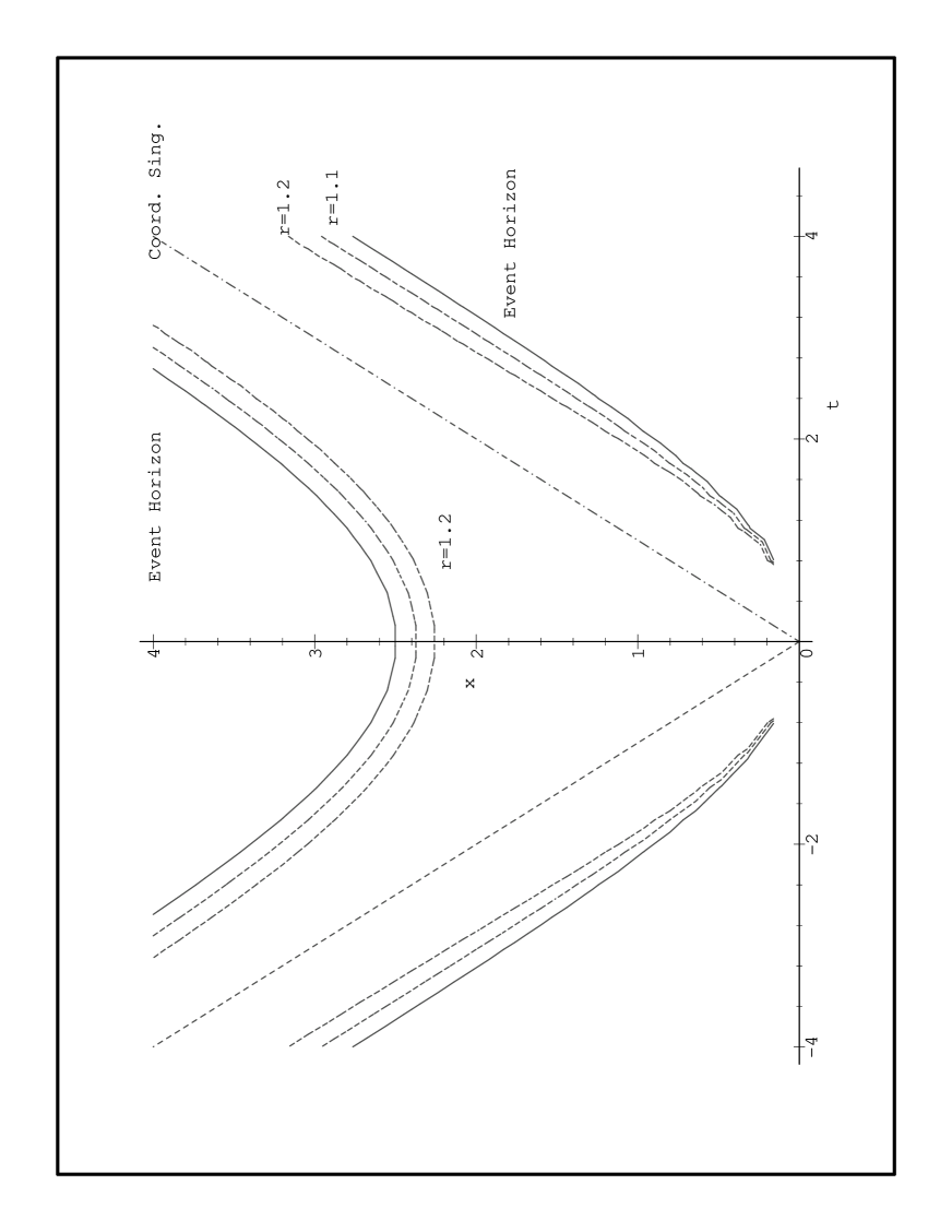
Figure 5: Horizons and coordinate singularity in 2-soliton coordinates.

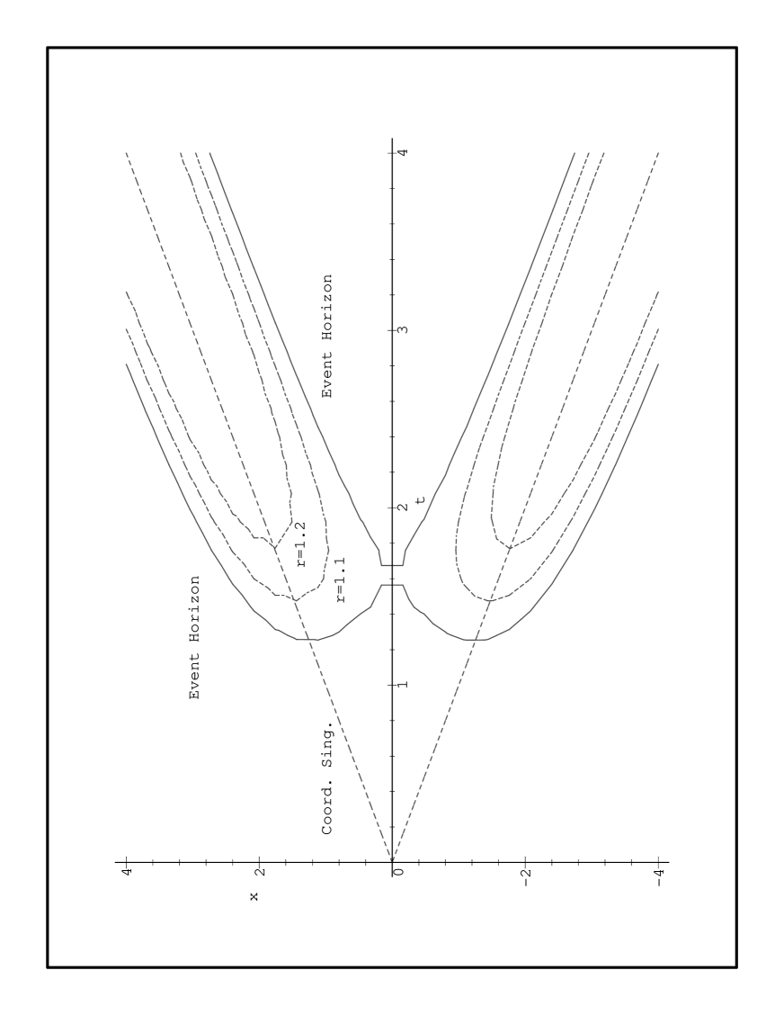
Figure 6: Horizons and coordinate singularities in soliton-anti-soliton coordinates.

It is interesting that this is again non-negative for all values of the soliton parameters. See Fig.5 for the structure of the horizons, coordinate singularities and some constant $\tau$ curves for the geometry in these coordinates. For the soliton-anti-soliton scattering solution, i.e. the case where $F,G$ are given by Eq.(57),Eq.(58), the expression for the dilaton is given by Eq.(73) but with $\sinh$ and $\cosh$ interchanged; while the expression for the conserved mass parameter is identical to Eq.(74) above. Fig.6 displays some of the geometrical features.

6 Hamiltonian Analysis

We now review the Hamiltonian analysis for Jackiw-Teitelboim gravity, using the notation of [14]. Spacetime is split into a product of space and time: $M_{2}\simeq\Sigma\times R$ and the metric $h_{\mu\nu}$ is given an ADM-like parameterization:[17]

$$ds^{2}=e^{\alpha}\left[-\sigma^{2}dt^{2}+\left(dx+Vdt\right)^{2}\right].$$ (75)

where $\alpha$, $V$ and $\sigma$ are functions on spacetime $M_{2}$. In the following, we denote by the overdot and prime, respectively, derivatives with respect to the time coordinate $t$ and spatial coordinate $x$.

The canonical momenta conjugate to the fields $\{\alpha,\tau\}$ are:

$$\Pi_{\alpha} = {1\over 2G\sigma}\left(V\tau^{\prime}-\dot{\tau}\right),$$ (76)

$$\Pi_{\tau} = {1\over 2G\sigma}\left(-\dot{\alpha}+V\alpha^{\prime}+2V^{\prime}\right),$$ (77)

The vanishing of the momenta canonically conjugate to $V$ and $\sigma$ yield the primary constraints for the system. Following the standard Dirac prescription[18], we obtain the canonical Hamiltonian (up to spatial divergences):

$$H_{0}=\int dx\left(V{\cal F}+{1\over 2G}\sigma{\cal G}\right).$$ (78)

where we have defined:

$${\cal F}:=\alpha^{\prime}\Pi_{\alpha}+\tau^{\prime}\Pi_{\tau}-2\Pi_{\alpha}^{\prime},$$ (79)

$${\cal G}:=2\tau^{\prime\prime}-\alpha^{\prime}\tau^{\prime}-\left(2G\right)^{2}\Pi_{\alpha}\Pi_{\tau}-2m^{2}{e^{\alpha}}\tau.$$ (80)

Clearly ${1\over 2G}\sigma$ and $V$ play the role of Lagrange multipliers that enforce the secondary constraints ${\cal F}\approx 0$ and ${\cal G}\approx 0$.

The energy can be constructed by noting that the following linear combination of the constraints is a total spatial derivative:

$$\tilde{\cal G} := {l\over 2}e^{-\alpha}\left((2G)^{2}\Pi_{\alpha}{\cal F}+\tau^{\prime}{\cal G}\right)$$ (81)

$$= (q[\alpha,\tau,\Pi_{\alpha},\Pi_{\tau}])^{\prime}$$

$$\approx 0,$$ (82)

where we have defined the variable $q$ as

$$q:={1\over 2m}\left[e^{-\alpha}\left((2G\Pi_{\alpha})^{2}-(\tau^{\prime})^{2}\right)+m^{2}\tau^{2}\right].$$ (83)

The expression on the right-hand side above is nominally an implicit function of the spatial coordinate, but is constant on the constraint surface. Moreover, it is straightforward to show that $q$ commutes with both constraints ${\cal F,G}$. Thus, the constant mode of $q$ is a physical observable in the Dirac sense.

In terms of the canonical momenta the magnitude of the Killing vector can be written as:

$$\mid k\mid^{2}={e^{-\alpha}\over m^{2}}\left[(2G\Pi_{\alpha})^{2}-(\tau^{\prime})^{2}\right]\,\,{}.$$ (84)

Thus the observable $q$ is:

$$q = {m\over 2}\left(\mid k\mid^{2}+\tau^{2}\right)$$ (85)

$$= {Mm\over 2}\,\,.$$

The momentum conjugate to $q$, is found by inspection to be[19]:

$$p:=-\int_{\Sigma}dx{2\Pi_{\alpha}e^{\alpha}\over(2G\Pi_{\alpha})^{2}-(\tau^{\prime})^{2}}\,\,.$$ (86)

The value of $p$ depends on the global properties of the spacetime slicing. This is consistent with the generalized Birkhoff theorem[19] which states that there is only one independent diffeomorphism invariant parameter characterizing the space of solutions.

It is instructive to write the observable $p$ in covariant form:

$$p = \int_{\Sigma}dxe^{\alpha/2}n^{\mu}{\nabla_{\mu}\tau\over\mid k\mid^{2}}$$ (87)

$$= -2\int_{\Sigma}dx^{\mu}{k_{\mu}\over\mid k\mid^{2}}$$ (88)

$$= -2m\int_{\sigma}dT.$$ (89)

Note that $dxe^{\alpha/2}$ is the measure induced on $\Sigma$ by $h_{\mu\nu}$. In the expression for $p$ the vector field $n^{\mu}$ is the unit (timelike) normal to $\Sigma$. The final expression is obtained by using the result Eq.(31), and proves explicitly that the momentum conjugate to $M$ is equal to the “Schwarzschild time separation” of the slice[20, 14].

The canonical Hamiltonian in terms of $\tilde{\cal G}$ is:

$$H_{0}=\int dx\left(\tilde{v}{\cal F}-\tilde{\sigma}{q^{\prime}\over G}\right)+H_{+}-H_{-}\,\,{}.$$ (90)

where $\tilde{v}=V-2G\sigma\Pi_{\alpha}/\tau^{\prime}$ and

$$\tilde{\sigma}={m\sigma e^{\alpha}\over\tau^{\prime}}.$$ (91)

Note that from Eq.(75) it follows that

$$\sigma e^{\alpha}=\sqrt{|g|}=|\sin(u/2)\cos(u/2)|$$ (92)

where the last expression is only valid in soliton coordinates. In Eq.(90) $H_{+}$ and $H_{-}$ are surface terms needed to make the variational principle well defined. These surface terms depend on the boundary conditions, and will be determined below.

We now impose boundary conditions on our spatial slice consistent with soliton coordinates Eq.(21). In particular, we assume that the spatial coordinate $x$ runs form $X_{-}=-\infty$ to $X_{+}=+\infty$. At the inner boundary $X_{-}$ the metric and dilaton should take on values corresponding to the asymptotic ($x\to-\infty$) region of a constant $t$ surface in soliton coordinates. As illustrated for the one-soliton case in Fig.4, such surfaces approach $\tau=0$ asymptotically along the horizon. Thus, we require $V_{-}\to 0$, $\sigma_{-}\to 0$, $\Pi_{\tau}|_{-}\to 0$, $e^{\alpha}|_{-}\to 1$, $\tau_{-}\to 0$ and $\tau^{\prime}_{-}\to 0$. However, in order for the Hamiltonian to be well defined, $\tilde{\sigma}$ must be finite at the boundary, so we restrict $\tilde{\sigma}_{-}=constant$. This condition has two important consequences. First it allows the boundary terms to be integrated in a straightforward fashion, as shown below. Secondly, once the soliton metric is specified, it fixes the scale of the dilaton. That is, given any soliton solution, there exists a corresponding black hole with uniquely determined mass. As we saw in Section 5, without this condition the linearity of the dilaton equations of motion allow an arbitrary multiplicative scale factor in the solution for the dilaton, and the resulting black hole mass observable is proportional to the square of the scale factor. However, in order to be able to impose this boundary condition on $\tilde{\sigma}$ it is necessary that $|\sin(u/2)\cos(u/2)|/\tau^{\prime}$ remain finite as $x\to-\infty$ for every soliton solution $u$ and dilaton field $\tau$. We have been able to verify this explicitly in the 1- and 2- soliton sector, but not in the general case. Specifically, in the one soliton case, for the solution given by Eq.(59) and Eq.(64) we find that $|\sin(u/2)\cos(u/2)|/\tau^{\prime}=1/(4m\gamma^{2})$ for all $x$, so we choose $a=1/(4m\gamma^{2})$ and the corresponding black hole mass is $M=v^{2}$ with corresponding ADM energy $E=mv^{2}/(2G)$. It is interesting that the ADM energy of the black hole is equal to the (non-relativistic) kinetic energy of the soliton.

In the two soliton case, one finds that

$$|\sin(u/2)\cos(u/2)|/\tau^{\prime}\to\left({v^{2}-1\over 2a}\right)\left[{|v\sin\mu\cos\mu|\over v}(1+v^{2})\right]^{-1},$$ (93)

as $x\to-\infty$, so we choose

$$a=\left({v^{2}-1\over 2}\right)\left[{|v\sin\mu\cos\mu|\over v}(1+v^{2})\right]^{-1},$$ (94)

to get a mass:

$$M=v^{2}\left[\cos^{2}\mu v^{2}-\sin^{2}\mu\over v^{2}-|v\sin\mu\cos\mu|(1+v^{2})\right].$$ (95)

The choice of boundary conditions at the outer boundary is somewhat more delicate. In order to consider black hole dynamics and thermodynamics we would like our spatial slice to include the asymptotic region of the black hole. Soliton coordinates, as discussed above, cannot be extended into the asymptotic region since there is a coordinate singularity at $u=(2n+1)\pi/2$, which corresponds to the location of a soliton. We avoid this problem by assuming that at $X_{+}\to\infty$, our spatial slice approaches asymptotically a static Schwarzschild slice, with no coordinate singularity between $X_{-}$ and $X_{+}$. This requires a change of coordinates between the horizon and the soliton location, since soliton coordinates are good in the neighbourhood of the horizon, while Schwarzschild coordinates are good in the neighbourhood of the soliton. As discussed in [14], the only boundary conditions that we require at $X_{+}$ are $\tilde{\sigma}_{+}\to 1$, $\tilde{v}_{+}\to 0$.

Given the above boundary conditions it is possible to evaluate the surface terms for any solitonic solution of the sine-Gordon equations. Using the identity:

$$\alpha^{\prime}\Pi_{\alpha}-2\Pi_{\alpha}^{\prime}=-{e^{\alpha}\over\Pi_{\alpha}}(e^{-\alpha}\Pi_{\alpha}^{2})^{\prime},$$ (96)

we first write the canonical Hamiltonian in the following form:

$$H_{0}=\int dx\left(-{\tilde{v}e^{\alpha}\over\Pi_{\alpha}}(e^{-\alpha}\Pi_{\alpha}^{2})^{\prime}+\tilde{v}\Pi_{\tau}\tau^{\prime}-\tilde{\sigma}{q^{\prime}\over G}\right)+H_{+}-H_{-}.$$ (97)

The variation of $H_{0}$ contains the following boundary terms:

$$\delta\left.H_{0}\right.|_{\hbox{boundary}}=\int dx\left(-{\tilde{v}e^{\alpha}\over\Pi_{\alpha}}\delta(e^{-\alpha}\Pi_{\alpha}^{2})+\tilde{v}\Pi_{\tau}\delta\tau-\tilde{\sigma}{\delta q\over G}\right)^{\prime}+\delta H_{+}-\delta H_{-}.$$ (98)

Given the above boundary conditions, potentially non-zero contributions are:

$$\delta H_{0}|_{\hbox{boundary}}=-\tilde{\sigma}\left.{\delta q\over G}\right|_{+}-\left.\left({\tilde{v}e^{\alpha}\over\Pi_{\alpha}}\delta(e^{-\alpha}\Pi_{\alpha}^{2})-\tilde{\sigma}{\delta q\over G}\right)\right|_{-}+\delta H_{+}-\delta H_{-}.$$ (99)

Using the expression for $q$ with for $\tau=\tau^{\prime}=0$, and the fact that when $V=0$, ${\tilde{v}e^{\alpha}\over\Pi_{\alpha}}=-\tilde{\sigma}$, we find that the there is no surface contribution at $X_{-}$, whereas the surface contribution in the asymptotic region can easily be integrated to give:

$$H_{+}=q/G={Mm\over 2G}.$$ (100)

7 Conclusions

We have discussed in some detail how Euclidean sine-Gordon solitons can be used to coordinatize black holes in Jackiw-Teitelboim gravity. The solitons appear as coordinate singularities that constitute the boundaries of the patches that can be faithfully coordinatized by the sine-Gordon coordinates. The horizons generically are regular in these coordinates. In the one-soliton case the soliton was a surface of constant dilaton field that lay just outside the horizon. There are still many unanswered questions about how our specific results for the 1- and 2- soliton sectors generalize to the N-soliton case.

Of course the most important question concerns whether or not there is any physics in this. It is tantalizing to speculate on what would happen if we were able to treat the solitons as physical particles propagating through the black hole spacetime, and providing a physical boundary whose deformations are in some way related to the diffeomorphisms of the horizon itself. Since in Carlip’s program [4] the diffeomorphisms of the horizon may be related to the black hole entropy, we might be able to quantize the horizon diffeos by quantizing the solitons and account for the black hole entropy by counting soliton states.

The following is evidence that such a proceedure may be worth pursuing. A black hole state has total energy $E_{0}$. Suppose it is described by an N-soliton solution of the sine-Gordon equation. (Ignore breathers and other exotica for now.) Ignoring breathers, etc., Takhtadjan and Faddeev [23] compute the total energy, valid both classically and quantum mechanically,

$$E=\sum_{i}^{N}\left(64m^{2}/\beta^{2}+p^{2}_{i}\right)^{1/2},$$ (101)

where $p_{i}$ is canonical momentum of $i^{th}$ lump and $\beta$ is the sine-Gordon coupling constant. Absorb factors of $64$ into $\beta^{-2}$, so the rest energy of the state is $E_{0}=mN/\beta$. Now combinatorics come in. The degeneracy of the state arises from the indistinguishability of the lumps in the N-soliton state. In other words, the degeneracy is the number of different ways to write N as the sum of non-negative integers. This is the number-theoretic partition function of Hardy-Ramanujan [24]

$$n(N)\sim e^{\pi\sqrt{2N/3}},$$ (102)

for large $N$. Hence the entropy behaves as

$$S\sim\log{n(N)}\sim\pi\sqrt{N}\sim\pi\sqrt{E_{0}}.$$ (103)

This is just the Bekenstein-Hawking entropy (up to factors of order 1) for a Jackiw-Teitelboim black hole of with total energy $E_{0}$.

This is quite sketchy, as well as speculative. In order to make the argument more rigorous, at least the following must be addressed:
(1.) Can one ignore breathers and other non-solitonic solutions of the sine-Gordon equation?
(2.) It is not obvious that the black hole energy is given by the rest energy of the N-soliton solution. It is true however that the energy of the black hole corresponding to a 1-soliton in the limit as the soliton parameter $v\to\infty$ is (up to numerical factors of order unity) the same as that of the 1-soliton itself.

Work is in progress to address these issues.

Acknowledgements

The authors would like to thank Y. Billig and M. Ryan for useful conversations. This work was supported in part by the Natural Sciences and Engineering Research Council of Canada. G.K is grateful to M. Ryan and A.A. Minzoni for helpful conversations.

Figure 1: Graph of soliton-soliton solution (solid line) and corresponding dilaton at (dashed line) fixed t (not to scale).

Figure 2: Graph of soliton-anti-soliton scattering solution (solid line) and corresponding dilaton(dashed line) for fixed t (not to scale).

Figure 3: Horizons and coordinate singularity in 1-soliton coordinates.

Figure 4: Surfaces of constant x (A..B..C..E) and t (F..G..H..I) in Kruskal coordinates.

References

- [1] For a review and references see, for example, J.-P. Luminet, ‘Black Holes: A General Introduction’, preprint astro-ph/9801252, to appear in Black Holes: Theory and Observation, Springer (1998).
- [2] For a review, see G. T. Horowitz, ‘Quantum States of Black Holes’, UCSBTH preprint UCSBTH-97-06, gr-qc/9704072 (1997).
- [3] A. Ashtekar, J. Baez, A. Corichi and K. Krasnov, Phys. Rev. Lett. 80, 904 (1998).
- [4] S. Carlip, Phys. Rev. D51, 632 (1995); hep-th/9806026 v2.
- [5] V. Frolov and D. Fursaev, hep-th/9806078.
- [6] See the contributions of R. Jackiw and C. Teitelboim in Quantum Theory of Gravity, ed. by S.M. Christensen, Adam Hilger, Bristol, (1984.)
- [7] M. Banados, C. Teitelboim and J. Zanelli, Phys. Rev. Lett. 69, 1849 (1992); M. Banados, M. Henneaux, C. Teitelboim and J. Zanelli, Phys. Rev. D48, 1506 (1993). M. Banados, ‘Constant Curvature Black Holes’, preprint gr-qc/9703040 (1997).
- [8] J.P.S. Lemos, Phys.Rev. D54, 6206 (1996).
- [9] For a review, see Solitons, Eds. R.K. Bullough, P.J. Caudrey (Springer-Verlag, Berlin, 1980); For references to the early work on sine-Gordon by Enneper, Bcklund, etc., see the contribution to this volume by R.K. Bullough.
- [10] L. Dolan, Phys. Rev. 15, 2337 (1977).
- [11] L.J. Boya and A.J. Segui-Santonja, J. Geom. Phys., 76 (1997).
- [12] J. Gegenberg and G. Kunstatter, Phys. Lett. B413, 274 (1997).
- [13] O. Babelon and D. Bernard, hep-th/9309154.
- [14] J. Gegenberg, G. Kunstatter and D. Louis-Martinez, Phys. Rev. D51, 1781 (1995).
- [15] R.B.Mann, Phys. Rev. D47,4438 (1993); J.P.S Lemos and P. Sá, Mod. Phys. Lett. A9, 771 (1994).
- [16] P.J. Caudrey, J.C. Eilbeck and J.D. Gibbon, Nuovo Cimento B25, 497 (1975).
- [17] C. G. Torre, Phys. Rev. D40, 2588 (1989).
- [18] P.A.M. Dirac, Lectures on Quantum Mechanics, Belfar Graduate School of Science (Yeshiva University, New York, 1964).
- [19] D. Louis-Martinez, J. Gegenberg and G. Kunstatter, Phys. Letts. B321, 193 (1994).
- [20] K. Kuchar, Phys. Rev. D50, 3913 (1994).
- [21] S. Bose L. Parker and Y. Peleg, Phys. Rev. D56, 987 (1997).
- [22] G. Kunstatter, R. Petryk, and S. Shelemy, Phys. Rev. D57, 3537 (1998).
- [23] L.A. Takhtadzhyan and L. D. Faddeev, Theor. and Math. Phys. 21, 1046 (1975).
- [24] S. Ramanujan and G.H. Hardy, Proc. London Math. Soc. (Ser. 2) 17, 75 (1918), reprinted in Collected Papers of Srinivase Ramanujan, ed. by G.H. Hardy, et. al., Celsea Pub. Co., NY (1962).