AEI-068

Varying the Unruh Temperature in
Integrable Quantum Field Theories
Max Niedermaier
Max-Planck-Institut für Gravitationsphysik

(Albert-Einstein-Institut)

Schlaatzweg 1, D-14473 Potsdam, Germany

Abstract

A computational scheme is developed to determine the response of a quantum field theory (QFT) with a factorized scattering operator under a variation of the Unruh temperature. To this end a new family of integrable systems is introduced, obtained by deforming such QFTs in a way that preserves the bootstrap S-matrix. The deformation parameter $\beta$ plays the role of an inverse temperature for the thermal equilibrium states associated with the Rindler wedge, $\beta=2\pi$ being the QFT value. The form factor approach provides an explicit computational scheme for the $\beta\neq 2\pi$ systems, enforcing in particular a modification of the underlying kinematical arena. As examples deformed counterparts of the Ising model and the Sinh-Gordon model are considered.

1. Introduction

Sometimes it is advantageous to step outside “flat land” Minkowski space quantum field theory (QFT) even if the quantity one is interested in concerns the latter. A good example is the conformal anomaly. In a $2n$-dimensional (flat space) QFT it can be defined through a coefficient of an $n+1$-point function of the energy momentum tensor. Technically however it is useful to first couple the system to some curved background and then compute the conformal anomaly as a suitable response with respect to a variation of the background metric (thereby producing the vacuum expectation value of the trace of the energy momentum tensor). Apart from the technical advantage that one only has to compute a 1-point function (in curved background) the result provides a linkage between flat space and curved space QFT.

1.1 Thermalization and Replica

Here we shall address the problem how to compute a similar response under a variation of the Unruh temperature. The latter refers to the well-known thermalization phenomenon that the vacuum of a Minkowski space QFT ‘looks like’ a thermal state of inverse temperature $\beta=2\pi$ (in natural units) with respect to the Killing time of the Rindler wedge [31, 4]. Heuristically one can summarize the result in the symbolic identity

$$\langle 0|{\cal O}_{1}(x_{1})\ldots{\cal O}_{n}(x_{n})|0\rangle={\rm Tr}[e^{2\pi K}{\cal O}_{1}(x_{1})\ldots{\cal O}_{n}(x_{n})]\;,\;\;\;\mbox{if}\;x_{1},\ldots,x_{n}\in W,$$ (1.1)

where $W$ is the right Rindler wedge, $K$ is the generator of Lorentz boosts in $W$ and ${\cal O}_{j}(x)$ are some local quantum fields. If we momentarily ignore the fact that the trace can never exist it is also clear what kind of operation one would like to perform, namely

$$\beta\frac{\partial}{\partial{\beta}}\,{\rm Tr}[e^{\beta K}\ldots]\,\Big{|}_{\beta=2\pi}\,,$$ (1.2)

with the understanding that ‘everything else’ is kept fixed (c.f. below). As in the case of the conformal anomaly such a response has two aspects. One is to define the systems with $\beta\neq 2\pi$, – which can no longer be ordinary Minkowski space QFTs. The other concerns the evaluation of the response itself, which again has significance within the context of Minkowski space QFT.

Let us now elucidate on the $\beta\neq 2\pi$ systems. There are two very different notions of “varying the Unruh temperature”:

• The classical notion of changing the norm of the timelike Killing vector field ${\cal K}$ in $W$ (and hence the surface acceleration $a$ of the Rindler horizon).

• The “replica” understanding of Callan and Wilczek [7] to replace $e^{2\pi K}$ in (1.1) with $(e^{2\pi K})^{\beta/2\pi}=e^{\beta K}$, keeping everything else (state space, operator products etc.) fixed.

There is a certain danger of confusing both notions because also the purely classical variation (a) affects the ($\hbar$-dependent) Unruh temperature $T=\frac{\hbar}{kc}\frac{a}{2\pi}$. To see this recall that in inertial coordinates ${\cal K}=a(x^{1}\partial_{0}+x^{0}\partial_{1})$, and its norm is $\|{\cal K}\|=a\sqrt{-x^{2}}$, using metric conventions $ds^{2}=(dx^{0})^{2}-(dx^{1})^{2}$ and $W=\{x\in\mbox{\rm IR}^{1,1}\,|\,|x^{0}|\leq x^{1}\}$. The result (1.1) holds in any dimension, for simplicity we specialize to 1+1 dimensions already at this point. Clearly ${\cal K}$ is unique up to normalization and changing its norm amounts to changing the Unruh temperature according to $T_{1}/T_{2}=\|{\cal K}_{1}\|/\|{\cal K}_{2}\|$. In particular (a) leaves the classical spacetime intact and thus is not the relevant concept if one wants to compute a quantum response of the form (1.2) or unravel the statistical origin of the Horizon entropy [5, 28, 7, 15, 16, 13]. Henceforth we shall exclusively be concerned with the notion (b) of varying the Unruh temperature. In order to disentangle both aspects we fix the norm of ${\cal K}$ once and for all to be $\|{\cal K}\|=\sqrt{-x^{2}}$. For the generator $K$ of the Lorentz boosts in the Minkowski space QFT this means

$$e^{i\lambda K}{\cal O}(x)e^{-i\lambda K}={\cal O}(x(\lambda))\;,\;\;\;\mbox{where}$$

$$x^{0}(\lambda)=x^{0}{\rm ch}\lambda+x^{1}{\rm sh}\lambda\;,\;\;\;x^{1}(\lambda)=x^{0}{\rm sh}\lambda+x^{1}{\rm ch}\lambda\;.$$ (1.3)

Note that with these normalizations a spacetime reflection corresponds to a complex Lorentz boost by $i\pi$.

Having fixed the normalization (1.3) the “replica” understanding of taking $\beta$ off $2\pi$ has the immediate consequence that one is no longer dealing with an ordinary QFT system. Taking again the heuristic formula (1.1) as a guideline one sees that translation invariance is broken: ${\rm Tr}[e^{\beta K}U(x){\cal O}U(x)^{-1}]={\rm Tr}[e^{\beta K}{\cal O}U(x)^{-1}U(x(-i\beta))]$, if $U(x)$ is the unitary representation of the translation group in the original QFT. Probably this should be viewed as the Minkowski space version of the conical singularity encountered in the Euclidean approach to the $\beta\neq 2\pi$ systems [10, 6, 21, 22].

1.2 Thermalization without event horizons

Here we shall pursue an approach to computing responses of the form (1.2) which preserves the Lorentzian signature and which implements the “replica” understanding of the $\beta\neq 2\pi$ systems on the level of form factors. It is based on a thermalization phenomenon related but not identical to (1.1) [24]. A schematic comparison of both phenomena is given in the table below.

Unruh Thermalization	Form Factor Thermalization
Hyperbolic World lines in	Mass hyperboloids in
Rindler space	forward light cone
$x^{0}=r\cosh\tau,\;\;x^{1}=r\sinh\tau$	$p_{0}=m\cosh{\theta},\;\;p_{1}=m\sinh{\theta}$
$\tau$: Killing time	$\theta$: rapidity
Wightman functions in	Form Factors in
Rindler space obey $(KMS)_{2\pi}$	Minkowski space obey $(KMS)_{2\pi}$
with respect to $\tau$	with respect to ${\theta}$

$(KMS)_{2\pi}$ denotes a thermal equilibrium condition of temperature $1/2\pi$ (with the normalization (1.3) and units $k=c=\hbar=1$). Mathematically, as first noticed by Kubo-Martin-Schwinger and Haag-Hugenholz-Winnink, the equilibrium condition gets encoded into certain analyticity properties with respect to some (generalized) time variable. The above form factor result has been shown to hold in any 1+1 dimensional QFT with a well-defined scattering theory, regardless of its integrability [24]. Form factors in this context are matrix elements of some field operator between the physical vacuum and the asymptotic multi-particle states. Let us denote the $n$-particle form factor of a field operator ${\cal O}$ symbolically by $\langle 0|{\cal O}|A(p_{n})\ldots A(p_{1})\rangle$, where $A(p)$ generates a 1-particle state of momentum $p=(m\cosh{\theta},m\sinh{\theta})$. Parallel to (1.1) one can give a mnemonic summary of the result as follows

$$\langle 0|{\cal O}|A(p_{n})\ldots A(p_{1})\rangle={\rm Tr}[e^{2\pi K}{\cal O}\,A(p_{n})\ldots A(p_{1})]\;.$$ (1.4)

Here $K$ is again the generator of Lorentz boosts and the comments from footnote 1 apply likewise. These technical aspects aside, it may come as a surprise that matrix elements of a zero temperature QFT exhibit thermal features, without an event horizon being invoked as in the Hawking-Unruh case. One explanation stems from the fact that the left hand side of (1.4) does not make essential use of the micro-causality property of the QFT, while the thermal structure of the right hand side can be understood as a ‘remnant of micro-causality’ on the level of scattering states. Another explanation can be gained from the strategy followed in the proof [24], which traces the thermalization in (1.4) back to that in the Bisognano-Wichmann-Unruh case [4, 31] by enclosing the ‘wave packets’ eventually forming the scattering states into ‘comoving’ wedge regions. In a forthcoming paper we study the generalization of (1.4) to higher dimensions.

Using (1.4) as a guideline it is easy to see what the replica understanding of $\beta\neq 2\pi$ amounts to. If we write $F({\theta}_{n},\ldots,{\theta}_{1})$ for $\langle 0|{\cal O}|A(p_{n})\ldots A(p_{1})\rangle$ the defining properties should be

$$F({\theta}_{n}+i\beta,{\theta}_{n-1},\ldots,{\theta}_{1})=\eta\,F({\theta}_{n-1},\ldots,{\theta}_{1},{\theta}_{n})\;,\;\;\;\mbox{and}$$

$$F({\theta}_{n},\ldots,{\theta}_{1})\;\;\mbox{has kinematical poles at}\;\;{\theta}_{k}-{\theta}_{j}=\pm i\pi\,,\,k\neq j\;.$$ (1.5)

The first equation is the $(KMS)_{\beta}$ condition where a generalized statistics phase $\eta$ may appear. The second requirement stems from ‘keeping everything else fixed’. In particular the normalization (1.3) should be kept fixed so that in the parameterization $p=(m\cosh{\theta},m\sinh{\theta})$ a sign flip still corresponds to a complex Lorentz boost by $i\pi$ rather than $i\beta/2$. This entails that the position of the kinematical singularities in rapidity space stay at ${\theta}_{k}-{\theta}_{j}=\pm i\pi$, $j\neq k$. Though (1.5) is a very natural transcription of the replica idea, it has a number of unexpected consequences. For example the spectra of the conserved charges on a multi-particle state change in a nontrivial way, c.f. section 3. The requirements (1.5) can be taken as the defining features for the $\beta\neq 2\pi$ systems in any 1+1 dim. QFT with a well-defined scattering theory. Very likely also a generalization to higher dimensions is possible. However the conditions are particularly stringent in so-called integrable QFTs on which we shall focus from now on.

By definition integrable massive QFTs are those for which the scattering operator enjoys a certain factorization property. This allows one to express all S-matrix elements in terms of the two-particle (“bootstrap”) S-matrix, which in turn is a solution of the Yang-Baxter equation. For such QFTs the so-called form factor approach allows one to characterize the full non-perturbative dynamical content of the QFT in terms of a recursive system of functional equations known as “form factor equations”. These functional equation only take the two-particle S-matrix as an input and are not renormalized or modified in any way in the process of solving the theory. Further they entail the quantum field theoretical locality requirement on the level of the Wightman functions [27]. It thus seems natural to modify this system of functional equations such that (1.5) is obeyed. It turns out that this can be done in a way that preserves the bootstrap S-matrix. For integrable QFTs therefore the concept of “keeping everything else fixed” in the replica understanding (b) of the $\beta\neq 2\pi$ systems acquires the precise meaning of: “Keeping the bootstrap S-matrix fixed”. Indeed, since ultimately the entire QFT gets constructed from it, changing the bootstrap S-matrix would amount to changing the theory. Remarkably with this specification mathematical consistency then dictates almost everything else [23]. Most importantly the residue equations have to be modified in a certain way. The sequences of meromorphic functions solving the modified functional equations no longer define the form factors of a relativistic QFT. We shall see:

• Each integrable QFT admits a 1-parameter deformation that preserves the bootstrap S-matrix. The deformation parameter $\beta$ plays the role of an inverse temperature in the “replica” understanding of taking $\beta$ off $2\pi$ in (1.4).

• The form factor approach provides an explicit computational scheme for these systems, just as for $\beta=2\pi$. It yields a finite, cutoff-independent answer for the response (1.2) of any local QFT quantity.

• For $\beta\neq 2\pi$ the underlying kinematical arena is deformed, but is by construction compatible with the full non-perturbative dynamics of the system. Lorentz invariance is maintained exactly.

The rest of this paper is organized as follows. In the next section we briefly describe the modified form factor equations and show that their solutions can have a regular $\beta\rightarrow 2\pi$ limit producing ordinary form factors. In section 3 we compute the spectrum of the conserved charges in the deformed theory with some details relegated to an appendix. Further the form factor resolution of the deformed two-point functions is introduced and its use illustrated for the energy momentum tensor of a free boson or fermion. In section 4 finally a few sample form factors in the deformed Ising model and Sinh-Gordon model are computed to demonstrate the feasibility of the scheme for interacting QFTs. The setting described bears some resemblance to ’t Hoofts “S-matrix Ansatz” [29, 30]. On this and other interrelations we briefly comment in the conclusions.

2. Deformed form factor equations

Let $S_{ab}^{cd}({\theta})$, ${\theta}\in\mbox{$\,${\sf I}{\bf C}}$, be a bootstrap S-matrix without bound state poles, i.e. a matrix-valued meromorphic function analytic in the strip $0\leq{\rm Im}\,{\theta}<\pi$ and satisfying the Yang-Baxter equation, unitarity and crossing. The indices $a,b,\ldots$ refer to a basis in some finite dimensional vector space $V$. Raising and lowering of indices is done by means of the charge conjugation matrix $C_{ab}$ and its inverse $C^{ab}$. To any such S-matrix one can associate a 1-parameter family of functional equations, whose solutions are sequences tensor-valued meromorphic functions [23]. The consistency of these equations is most conveniently seen in an algebraic implementation. Here we shall give only a minimal set of equations, which – taken for granted the consistency of the deformation – entail all others. For generic $\beta\neq 2\pi$ thus consider the following set of functional equations [23]

$$F_{a_{n}\ldots a_{1}}({\theta}_{n}+i\beta,{\theta}_{n-1},\ldots,{\theta}_{1})=\eta\,F_{a_{n-1}\ldots a_{1}a_{n}}({\theta}_{n-1},\ldots,{\theta}_{1},{\theta}_{n})\;,$$ (2.1)

$$F_{a_{n}\ldots a_{1}}({\theta}_{n},{\theta}_{n-1},\ldots,{\theta}_{1})=S_{a_{n}a_{n-1}}^{d\;\;c}({\theta}_{n,n-1})\,F_{c\,da_{n-2}\ldots a_{1}}({\theta}_{n-1},{\theta}_{n},{\theta}_{n-2}\ldots,{\theta}_{2},{\theta}_{1})$$ (2.2)

$$\mbox{Res}\,F^{(n)}_{A}({\theta}_{n-1}+i\pi,{\theta}_{n-1},{\theta}_{n-2},\ldots,{\theta}_{1})=-\lambda^{-}C_{a_{n}a_{n-1}}\,F^{(n-2)}_{a_{n-2}\ldots a_{1}}({\theta}_{n-2},\ldots,{\theta}_{1})\;.$$ (2.3)

For ${\theta}_{n}={\theta}_{n-1}-i\pi$ one has

$$\mbox{Res}\,F^{(n)}_{A}({\theta}_{n-1}-i\pi,{\theta}_{n-1},{\theta}_{n-2},\ldots,{\theta}_{1})=-\lambda^{+}C_{a_{n}a_{n-1}}\,F^{(n-2)}_{a_{n-2}\ldots a_{1}}({\theta}_{n-2},\ldots,{\theta}_{1})\;,$$

$$\mbox{Res}\,C^{a_{n}a_{n-1}}F^{(n)}_{A}({\theta}_{n-1}-i\pi,{\theta}_{n-1},{\theta}_{n-2},\ldots,{\theta}_{1})=-\lambda^{-}\,F^{(n-2)}_{a_{n-2}\ldots a_{1}}({\theta}_{n-2},\ldots,{\theta}_{1})\;.$$ (2.4)

The first version applies to a $2\pi i$-periodic S-matrix, the second when $S_{ab}^{cd}(-i\pi)$ is singular. Here and below “Res” denotes the residue at the simple pole of the displayed pair of rapidities, here: $\mbox{Res}=\mbox{res}_{{\theta}_{n}={\theta}_{n-1}\pm i\pi}$. Further $A=(a_{n},\ldots,a_{1})$, ${\theta}=({\theta}_{n},\ldots,{\theta}_{1})$ and we use the shorthand ${\theta}_{kj}:={\theta}_{k}-{\theta}_{j}$ throughout. The constants $\lambda^{-}=-i\beta/\pi,\;\lambda^{+}=\lambda^{-}/\dim V$ are chosen to match the normalization of the 1-particle states ${}_{b}\langle{\theta}_{2}|{\theta}_{1}\rangle_{a}=2\beta\delta_{ba}\delta({\theta}_{21})$, and $\eta$ is a complex phase. In addition to the equations (2.3.a-d) of course one has to specify the analytic structure of the solutions aimed at. For $\beta/2\pi$ irrational we require the solutions of (2.3.a,b) to be meromorphic functions with poles at most at ${\theta}_{kj}=\pm i\pi$ modulo $i\beta$; in particular they are supposed to be regular at ${\theta}_{j+1,j}=i\beta$. The equations (2.3.c,d) then serve to arrange the solutions of (2.3.a,b) into sequences. One aspect of the consistency alluded to before is that the operations ‘application of a symmetry transformation’ via (2.3.a,b) and ‘taking the residue’ via (2.3.c,d) commute. In particular this implies that any solution of (2.3.a,b) having a simple pole at ${\theta}_{n}={\theta}_{n-1}\pm i\pi$ will have simple poles also at ${\theta}_{j+1,j}=\pm i\pi$ and ${\theta}_{j+1,j}=\mp i(\pi-\beta)$, whose residues are given by

$$\mbox{Res}\,F^{(n)}_{A}({\theta}_{n},\ldots,{\theta}_{j}+i\pi,{\theta}_{j},\ldots,{\theta}_{1})$$

$$\makebox[28.45274pt]{ }=-\lambda^{-}C_{a_{j+1}a_{j}}\,F^{(n-2)}_{a_{n}\ldots a_{j+2}a_{j-1}\ldots a_{1}}({\theta}_{n},\ldots,{\theta}_{j+2},{\theta}_{j-1},\ldots,{\theta}_{1})\;,$$ (2.6)

$$\mbox{Res}\,F^{(n)}_{A}({\theta}_{n},\ldots,{\theta}_{j}-i\pi+i\beta,{\theta}_{j},\ldots,{\theta}_{1})$$

$$\makebox[28.45274pt]{ }=-\lambda^{+}\,L_{t_{j+1}}({\theta}_{n},\ldots,{\theta}_{j}-i\pi+i\beta,{\theta}_{j},\ldots,{\theta}_{1})_{A}^{B}\;C_{b_{j+1}b_{j}}\,F^{(n-2)}_{p_{j}B}(p_{j}{\theta})\;,$$ (2.7)

and similar equations for ${\theta}_{j+1,j}=-i\pi$ and ${\theta}_{j+1,j}=i(\pi-\beta)$. The notation is $p_{j}A=(a_{n},\dots a_{j+2}a_{j-1}\ldots a_{1})$ and $p_{j}{\theta}=({\theta}_{n},\ldots,{\theta}_{j+2},{\theta}_{j-1},\ldots,{\theta}_{1})$. Further

$$L_{\tau_{j}}({\theta})_{A}^{B}=\eta\,T_{a_{j}}^{c}({\theta}_{j}|{\theta}_{n},\ldots,{\theta}_{j+1})^{b_{n}\ldots b_{j+1}}_{a_{n}\ldots a_{j+1}}\;T_{c}^{b_{j}}({\theta}_{j}-i\beta|{\theta}_{j-1},\ldots,{\theta}_{1})_{a_{j-1}\ldots a_{1}}^{b_{j-1}\ldots b_{1}}\;,$$ (2.9)

is the matrix entering the deformed Knizhnik-Zamolodchikov equations; the corresponding action on rapidity vectors is $\tau_{j}({\theta}_{n},\ldots,{\theta}_{1})=({\theta}_{n},\ldots,{\theta}_{j}+i\beta,\ldots,{\theta}_{1})$. As indicated it can be expressed in terms of the monodromy matrix

$$T_{a_{n}}^{b_{n}}({\theta}_{n}|{\theta}_{n-1},\ldots,{\theta}_{1})_{a_{n-1}\ldots a_{1}}^{b_{n-1}\ldots b_{1}}=S_{c_{n-1}a_{n-1}}^{b_{n}b_{n-1}}({\theta}_{n-1,n})\;S_{c_{n-1}a_{n-2}}^{c_{n-2}b_{n-2}}({\theta}_{n-2,n})\;\ldots\;S_{a_{n}a_{1}}^{c_{2}b_{1}}({\theta}_{1,n})\;,$$

whose trace over $a_{n}=b_{n}$ yields the well-known family of commuting operators on $V^{\otimes(n-1)}$.

The dependence on $\beta$ in the deformed form factors will usually be suppressed. When needed to distinguish them from the undeformed form factors we shall write $(F^{(\beta,n)})_{n\geq 0}$ and $(F^{(2\pi,n)})_{n\geq 0}$ for the deformed and undeformed ones, respectively. In this notation one can select solutions for generic $\beta$ such that

$$F^{(2\pi,n)}_{A}({\theta})=\lim_{\beta\rightarrow 2\pi}F_{A}^{(\beta,n)}({\theta})\;.$$ (2.10)

To verify this one has to show that the right hand side solves the undeformed form factor equations. For the equations (2.3.a,b) this is obvious. To see that the residue equations come out correctly observe that in the limit $\beta\rightarrow 2\pi$ the poles at ${\theta}_{j+1,j}=i\pi$ and ${\theta}_{j+1,j}=i(\beta-\pi)$ in (2.7) merge. They produce a simple pole again because by assumption $F^{(\beta,n)}_{A}({\theta})$ does not have a pole at ${\theta}_{j+1,j}=i\beta$. In particular this implies that the residues of the merged poles add up producing

$$\mbox{Res}\,F^{(n)}_{A}({\theta}_{n},\ldots,{\theta}_{j}+i\pi,{\theta}_{j},\ldots,{\theta}_{1})$$

$$\makebox[28.45274pt]{ }=-\left[\lambda^{+}L_{\tau_{j+1}}({\theta}_{n},\ldots,{\theta}_{j}+i\pi,{\theta}_{j},\ldots,{\theta}_{1})_{A}^{B}\;+\lambda^{-}\delta_{A}^{B}\right]\,C_{b_{j+1}b_{j}}F^{(n-2)}_{p_{j}B}(p_{j}{\theta})\;,$$ (2.11)

which is the undeformed residue equation. In principle it is non-trivial that solutions of the deformed equations exist such that (2.10) is satisfied. Based on experience with the simple models described later, we expect however the following to be true:

• For each ordinary form factor sequence $(F^{(2\pi,n)})_{n\geq 1}$ there exists a deformed counterpart $(F^{(\beta,n)})_{n\geq 1}$ such that (2.10) is satisfied.

• The deformed sequence is in general not uniquely specified by (2.10) but can be made so by imposing suitable minimality conditions.

Naturally one will search for solutions of the deformed equations with a definite degree of homogeneity $s$ (“spin”) under the action of $e^{i\lambda K}$, $iK=\sum_{j}\frac{\partial}{\partial{\theta}_{j}}$. In the undeformed case suitable multiplets of solutions then transform according to tensor representations of SO(1,1), reflecting the Lorentz covariance properties of the local operator assigned to it. The same can be done here, though a-priori without any reference to an underlying QFT system. For example an appropriate triplet of solutions $F_{s}^{(n)}({\theta})$ of spin $s=0,\pm 2$ can be used to define a symmetric second rank SO(1,1) tensor $F_{\mu\nu}^{(n)}({\theta})$,

$$F^{(n)}_{\mu\nu}({\theta}_{n}+\lambda,\ldots,{\theta}_{1}+\lambda)=\Lambda(\lambda)_{\mu}^{\;\rho}\Lambda(\lambda)_{\nu}^{\;\sigma}\,F^{(n)}_{\rho\sigma}({\theta})\;,$$

$$\Lambda(\lambda)_{\mu}^{\;\nu}=\left(\begin{array}[]{cc}{\rm ch}\frac{2\pi}{\beta}\lambda&{\rm sh}\frac{2\pi}{\beta}\lambda\\ {\rm sh}\frac{2\pi}{\beta}\lambda&{\rm ch}\frac{2\pi}{\beta}\lambda\end{array}\right)\;,\;\;\;\mu,\nu=0,1\;,$$ (2.14)

where the components $F_{\mu\nu}^{(n)}({\theta})$ are linear combinations of $F_{s}^{(n)}({\theta})$, $s=0,\pm 2$.

3. Deformed kinematics

The structure of the deformed kinematics turns out to be largely dictated by consistency with the dynamics, i.e. with the deformed form factors equations. In this section we present some aspects of the resulting kinematics.

3.1 Deformed conserved charges

In the undeformed case local conserved charges are characterized by two properties. They act numerically on asymptotic multi-particle states and their eigenvalues decompose into a sum of 1-particle contributions. On the level of form factors, the first property implies that the eigenvalues are trivial solutions of the form factor equations. Here we take the (deformed) form factor equations as the starting point, so that it is natural to define a conserved charge in terms of its eigenvalues as follows: A conserved charge $Q_{s}$ of spin $s$ has eigenvalues $Q_{s}^{(n)}({\theta})$ that are real for real arguments, $i\beta$-periodic and symmetric in all variables, as well as homogeneous and hermitian in the following sense

$$Q_{s}^{(n)}({\theta}_{n}+\lambda,\ldots,{\theta}_{1}+\lambda)=e^{s\frac{2\pi}{\beta}\lambda}\,Q_{s}^{(n)}({\theta})\;,\makebox[28.45274pt]{ }Q_{s}^{(n)}({\theta})^{*}=Q_{s}^{(n)}({\theta}^{*})\;.$$ (3.1)

Further the eigenvalues for $n$ and $n-2$ particles are linked by the recursive relation

$$Q_{s}^{(n)}({\theta}_{n}={\theta}_{n-1}\pm i\pi,{\theta}_{n-1},{\theta}_{n-2},\ldots,{\theta}_{1})=Q_{s}^{(n-2)}({\theta}_{n-2},\ldots,{\theta}_{1})\;.$$ (3.2)

In summary a conserved charge in the deformed theory is in correspondence to a sequence $(Q_{s}^{(n)}({\theta}))_{n\geq 0}$ of symmetric functions solving (3.1), (3.2). The structure of the solutions turns out to be quite different from that for $\beta=2\pi$. Intrinsically however the role of the deformed eigenvalue sequences is precisely the same as in the undeformed case: Pointwise multiplication of a given form factor sequence with $(Q_{s}^{(n)}({\theta}))_{n\geq 0}$ produces a new form factor sequence (with spin $s+s^{\prime}$, if the original sequence had spin $s^{\prime}$). Clearly the set of eigenvalue sequences forms a graded abelian ring with respect to pointwise addition and multiplication, where upon multiplication the degrees add up. In a theory whose S-matrix has bound state poles the recursion relation (3.2) will be supplemented by a $n\rightarrow n-1$ recursive relation, which in particular serves as a selection principle for the allowed spin values. Here we shall restrict attention to S-matrices without bound state poles. In particular the mass gap $m$ then provides the only intrinsic mass scale of the theory.

For $\beta=2\pi$ the most important solutions of (3.1), (3.2) are the “power sums” $P_{s}^{(n)}({\theta})\sim t_{1}^{s}+\ldots+t_{n}^{s}$ for $s$ odd and $t_{j}=e^{{\theta}_{j}}$. In fact these powers sums form a basis for the before-mentioned “ring of conserved charges” at $\beta=2\pi$ [9]. That is to say all other solutions of (3.1), (3.2) are linear combinations of products of the power sums. In physical terms $P_{\pm 1}^{(n)}({\theta})$ for example are (up to a normalization constant with units of a mass) the eigenvalues of the lightcone momenta $P_{\pm}$ on an asymptotic $n$-particle state. Their product $P_{+1}^{(n)}({\theta})P_{-1}^{(n)}({\theta})$ is proportional to the $n$-particle eigenvalues of the $(\rm{mass})^{2}$ operator $2P_{+}P_{-}$. Observe also that the power sums (and their linear combinations) are distinguished by the property that for them the rapidities provide an additive parameterization of the multi-particle eigenvalues

$$P_{s}^{(n)}({\theta})=\sum_{j}P_{s}^{(1)}({\theta}_{j})\;.$$ (3.3)

For $\beta\neq 2\pi$ such solutions of (3.1), (3.2) no longer exist. Nevertheless natural deformed counterparts of the power sums do exist and they will play a key role in the following.

The starting point for the construction of the deformed power sums is the following fact: Let $P^{(n)}(N,l)$ be the space of symmetric polynomials in $t_{1},\ldots,t_{n}$ of total degree $N$ and partial degree $l$ (c.f. Appendix). There exists a unique sequence of $i\beta$-periodic symmetric functions $(P^{(n)}(t))_{n\geq 0}$ such that

• $P^{(n)}(t)$ is a ratio of symmetric polynomials in $t_{j}=e^{2\pi{\theta}_{j}/\beta}$, $1\leq j\leq n$, solving (3.1), (3.2). The numerator ${\rm num}P^{(n)}$ and denominator ${\rm den}P^{(n)}$ have the following degrees

  $${\rm num}P^{(n)}\in P^{(n)}(N+1,n)\;,\;\;\;{\rm den}P^{(n)}\in P^{(n)}(N,n-1)\;,\;\;\;N=\frac{1}{2}n(n-1)\;.$$ (3.4)

• $P^{(n)}(t)$ is proportional to the eigenvalue of the $P_{+}$ lightcone momentum operator for $\beta\rightarrow 2\pi$, i.e.

  $$P^{(n)}(t)\bigg{|}_{\beta=2\pi}=t_{1}+\ldots+t_{n}\;.$$ (3.5)

Further no solution of the same type with lower degrees in (3.4) exists. Here and later on it will be convenient to express all symmetric polynomials in terms of the elementary symmetric polynomials $\sigma_{k}^{(n)}$, $k=1,\ldots,n$ (where we shall usually suppress the superscripts $n$). Writing further $\gamma=2\cos\frac{\pi^{2}}{\beta}$ and ${\delta}=2\cos\frac{2\pi^{2}}{\beta}=q+q^{-1}=\gamma^{2}-2$, the explicit results for $n\leq 4$ are:

$${\rm num}P^{(2)}=\sigma_{1}^{2}-\gamma^{2}\sigma_{2}\;,\makebox[28.45274pt]{ }{\rm den}P^{(2)}=\sigma_{1}\;,$$

$${\rm num}P^{(3)}=\sigma_{1}^{2}\sigma_{2}-\gamma^{2}\sigma_{2}^{2}+(1+{\delta})\sigma_{1}\sigma_{3}\;,$$

$${\rm den}P^{(3)}=\sigma_{1}\sigma_{2}-(1+{\delta})^{2}\,\sigma_{3}\;,$$

$${\rm num}P^{(4)}=\sigma_{1}^{2}\sigma_{2}\sigma_{3}-\gamma^{2}\,\sigma_{2}^{2}\sigma_{3}+(1+{\delta})\sigma_{1}\sigma_{3}^{2}-(1+{\delta})^{2}\sigma_{1}^{3}\sigma_{4}$$

$$\makebox[56.9055pt]{ }+{\delta}\gamma^{4}\,\sigma_{1}\sigma_{2}\sigma_{4}-{\delta}^{2}\gamma^{2}(1+{\delta})\,\sigma_{3}\sigma_{4}\;,$$

$${\rm den}P^{(4)}=\sigma_{1}\sigma_{2}\sigma_{3}-(1+{\delta})^{2}(\sigma_{3}^{2}+\sigma_{1}^{2}\sigma_{4})+{\delta}\gamma^{4}\,\sigma_{2}\sigma_{4}\;.$$ (3.6)

The most efficient way to compute these expressions is by making use of the fact that both the numerators and the denominators separately obey a recursive relation. These and other aspects of the construction of the conserved charge eigenvalues are relegated to the Appendix. Clearly the solutions (3.6) violate (3.3). Nevertheless one can recover an additive parameterization by means of the following result.

Lemma: Let $P^{(n)}(t)$ be the functions defined above. Set

$$l_{j}^{(n)}(t):=t_{j}\frac{\partial}{\partial{t_{j}}}P^{(n)}(t)\;,\;\;\;j=1,\ldots,n\;,$$ (3.7)

which by construction reduce to $t_{j}$ for $\beta=2\pi$. Then

$$P_{s}^{(n)}(t):=[l_{1}^{(n)}(t)]^{s}+\ldots+[l_{n}^{(n)}(t)]^{s}\;,$$ (3.8)

is a conserved charge eigenvalue for all (positive and negative) odd integers $s$, which for $\beta=2\pi$ reduces to $t_{1}^{s}+\ldots+t_{n}^{s}$.

The point here is that the expressions (3.8) again solve the recursive equation (3.2). For $s=1$ this is just a rewriting of the Euler relation, but for $s\neq 1$ the proof is more involved. We omit it. Clearly the $P_{s}^{(n)}(t)$ are natural deformed counterparts of the power sums. They are again expressible as ratios of homogeneous symmetric polynomials, though usually of a fairly high (total and partial) degree.

Let us focus now on the $s=\pm 1$ conserved charges. A drawback of the construction (3.7), (3.8) is that the $s=1$ and the $s=-1$ charges enter asymmetrically. To understand how this comes about consider $P^{(n)}(t^{-1})$ with $t^{-1}=(t_{n}^{-1},\ldots,t_{1}^{-1})$, which meets the same requirements as $P_{-1}^{(n)}(t)$: It solves (3.1), (3.2) with $s=-1$ and reduces to $t_{n}^{-1}+\ldots+t_{1}^{-1}$ for $\beta=2\pi$. In terms of the elementary symmetric polynomials the inversion $t\rightarrow t^{-1}$ amounts to the replacement $\sigma_{k}\rightarrow\sigma_{n-k}/\sigma_{n}$. The functions $P^{(n)}(t^{-1})$ are thus again expressible as ratios of symmetric polynomials in $t_{1},\ldots,t_{n}$ with degrees readily worked out from (3.4). If we next consider the sequence of ratios

$$Q^{(n)}(t):=\frac{P_{-1}^{(n)}(t)}{P^{(n)}(t^{-1})}\;,\makebox[28.45274pt]{ }Q^{(n)}(t)\bigg{|}_{\beta=2\pi}=1\;,\;\;n\geq 1\;,$$ (3.9)

its members qualify as spin zero solutions of (3.1), (3.2) starting with $Q^{(0)}=1/(4-\gamma^{2})$ and $Q^{(1)}=1$. In other words the $s=1$ and $s=-1$ power sums in (3.8) feature asymmetrically only because one of them has been multiplied with a complicated spin zero conserved charge having trivial $\beta=2\pi$ limit. It is obviously nicer to distribute the square root of $Q^{(n)}(t)$ symmetrically on both the $s=1$ and the $s=-1$ power sums. This leads us to the following definition of the deformed lightcone momentum eigenvalues

$$k_{j}^{(n)}(t):=[Q^{(n)}(t)]^{1/2}\,l_{j}^{(n)}(t)\;,\;\;\;j=1,\ldots,n\;,$$

$$P_{+}^{(n)}(t):=\frac{m}{\sqrt{2}}\sum_{j=1}^{n}k_{j}^{(n)}(t)=\frac{m}{\sqrt{2}}[Q^{(n)}(t)]^{1/2}\,P^{(n)}(t)\;,$$

$$P_{-}^{(n)}(t):=\frac{m}{\sqrt{2}}\sum_{j=1}^{n}[k_{j}^{(n)}(t)]^{-1}=\frac{m}{\sqrt{2}}[Q^{(n)}(t)]^{1/2}\,P^{(n)}(t^{-1})\;,$$ (3.10)

where $m$ is the mass gap. In particular in this way an additive parameterization and a standard relativistic dispersion relation are recovered. Of course one would like to interpret $k_{j}^{(n)}(t)$ as the lightcone momentum of the $j$-th particle in an $n$-particle state of the deformed theory. For this to be possible the $k_{j}^{(n)}(t)$ should better be non-negative functions on $\mbox{\rm IR}_{+}^{n}$. For sufficiently small $\gamma$ one expects this to work out, but it is not obvious how large $\gamma$ can be made without sacrificing this property. From the explicit expressions we verified that for $n\leq 4$

$$k_{j}^{(n)}(t)\geq 0\;,\;\;\forall t\in\mbox{\rm IR}_{+}^{n}\;\;\;\mbox{if}\;\;\gamma^{2}<1\,.$$ (3.11)

In fact it is sufficient to check (3.11) for the $l_{j}^{(n)}(t)$, because then also $Q^{(n)}(t)$ is nonnegative for $\gamma^{2}<1$. We expect (3.11) to be a generic feature and henceforth restrict attention to $-1<\gamma<1$, i.e. to $\frac{3}{4}<|\frac{\beta}{2\pi}|<\frac{3}{2}$.

A natural definition of the deformed mass eigenvalues is

$$M^{(n)}(t)=[2P_{+}^{(n)}(t)P_{-}^{(n)}(t)]^{1/2}\;.$$ (3.12)

They are conserved charges with the correct $\beta\rightarrow 2\pi$ limit. In addition their threshold values are the same as in the undeformed case, i.e. $M^{(n)}(t)\geq nm$, $\forall t\in\mbox{\rm IR}_{+}^{n}$, and equality only holds on the main diagonal of $\mbox{\rm IR}^{n}_{+}$. Off the diagonal however the deformed mass eigenvalues are always larger than the undeformed ones. If we regard (3.12) as a function $M^{(n)}(u)$ of the rapidity differences $u_{i}=\frac{2\pi}{\beta}({\theta}_{i+1}-{\theta}_{i})$, $i=1,\ldots,n-1$, this amounts to

$$M^{(n)}(u)\geq m\left[n+2\sum_{i<j}{\rm ch}(u_{i}+\ldots+u_{j})\right]^{1/2}=M^{(n)}(u)\bigg{|}_{\beta=2\pi}\;,$$ (3.13)

where for $u_{i}\neq 0$ strict inequality holds. In physical terms (3.13) means that boosting two particles relative to each other costs more energy than in the undeformed case. The price can be measured in units of the undeformed energy, i.e. in terms of the ratio $M^{(n)}(u)/[M^{(n)}(u)]_{\beta=2\pi}$. The resulting cost functions have a global minimum at $u=0$ and local minima in the form of ‘valleys’ in the vicinity of the diagonals where two or more rapidities coincide. Off the diagonals the ratio quickly approaches a constant value. The height $h$ of this plateau rapidly increases with $n$ and $|\gamma|$. For example at $\gamma=0.9$ one has $h\approx 2.3,\,5.2,\,12$, for $n=2,3,4$, respectively. For $n=3$ and $\gamma=0.9$ the surface of the relative energy costs is shown in Figure 1. For other values of $0<|\gamma|<1$ the surfaces are qualitatively similar.

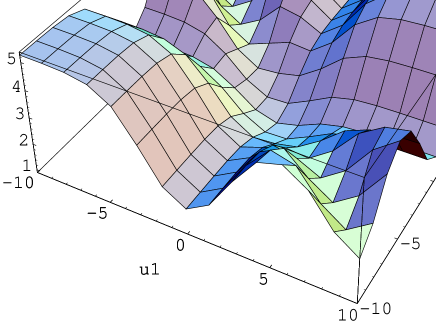
Figure 1: Ratio of the deformed and undeformed three-particle mass eigenvalues $M^{(3)}(u_{1},u_{2})/[M^{(3)}(u_{1},u_{2})]_{\beta=2\pi}$ for $\gamma=2\cos\pi^{2}/\beta=0.9$.

3.2 Rapidity diffeomorphisms

The positivity (3.11) also allows one to introduce single valued ‘physical’ rapidities $\alpha_{j}$ carrying an induced action of Lorentz boosts

$$\alpha_{j}^{(n)}({\theta}):=\frac{\beta}{2\pi}\ln k_{j}^{(n)}(t)\;,\;\;\;\alpha_{j}^{(n)}({\theta}_{n}+\lambda,\ldots,{\theta}_{1}+\lambda)=\lambda+\alpha_{j}^{(n)}({\theta})\;.$$ (3.14)

The mapping $\mbox{\rm IR}^{(n)}_{+}\rightarrow\mbox{\rm IR}^{(n)}_{+},(t_{n},\ldots,t_{1})\rightarrow(k_{n},\ldots,k_{1})$ is obviously differentiable and the Hessian can be checked to be nonsingular. Thus geometrically (3.14) provides a diffeomorphism

$$\mbox{\rm IR}^{n}\ \longrightarrow\ \mbox{\rm IR}^{n},\;\;\;({\theta}_{n},\ldots,{\theta}_{1})\ \longrightarrow\ (\alpha_{n},\ldots,\alpha_{1})\;,$$ (3.15)

from the real ‘form factor’ rapidities ${\theta}_{j}$ to the real ‘physical’ rapidities $\alpha_{j}$. The former have the virtue that in terms of them form factors, conserved charge eigenvalues etc. admit an analytic continuation with controllable analyticity properties, which moreover adhere to the “replica” understanding of taking $\beta\neq 2\pi$. However they do not provide an additive parameterization of energy and momentum on a multi-particle state. The latter can be achieved by switching to the rapidities $\alpha_{j}$ at the expense of a vastly more complicated structure of nontrivial form factors. (For example the form factors constructed in section 4 re-expressed in terms of the $k_{j}$’s would be horrendous). Technically it is therefore convenient to work with the ‘form factor’ rapidities ${\theta}_{j}$ throughout taking into account the Jacobian stemming from (3.15). For the resolution of the identity in terms of multi-particle states this means

11 $$\!=\! \sum_{n}\frac{1}{n!}\int\frac{d^{n}\alpha}{(2\beta)^{n}}|\alpha_{n},\ldots,\alpha_{1}\rangle\langle\alpha_{1},\ldots,\alpha_{n}|$$ (3.16)

$$\!=\! \sum_{n}\frac{1}{n!}\int\frac{d^{n}{\theta}}{(2\beta)^{n}}\,\Omega^{(n)}({\theta})|{\theta}_{n},\ldots,{\theta}_{1}\rangle\langle{\theta}_{1},\ldots,{\theta}_{n}|\;.$$

Since the form factors considered later will be functions of $t_{j}=e^{2\pi{\theta}_{j}/\beta}$ only it is convenient to also treat the Jacobian as a function $\Omega^{(n)}(t)$ of the $t_{j}$’s. This gives

$$\int\frac{d^{n}\alpha}{(2\beta)^{n}}=\int\frac{d^{n}k}{(4\pi)^{n}}\frac{1}{k_{1}\cdots k_{n}}=\int\frac{d^{n}t}{(4\pi)^{n}}\frac{\Omega^{(n)}(t)}{t_{1}\cdots t_{n}}=\int\frac{d^{n}{\theta}}{(2\beta)^{n}}\,\Omega^{(n)}({\theta})\;,$$ (3.17)

where the integrals are over $\mbox{\rm IR}^{n}$ or $\mbox{\rm IR}_{+}^{n}$ and

$$\Omega^{(n)}(t)=\frac{t_{1}\ldots t_{n}}{k_{1}^{(n)}\ldots k_{n}^{(n)}}\;\det\left(\frac{\partial k^{(n)}_{i}}{\partial t_{j}}\right)_{1\leq i,j\leq n}\;.$$ (3.18)

As indicated we write $\Omega^{(n)}({\theta})$ for $\Omega^{(n)}(t)$ when regarding the Jacobian as a function of the rapidities rather than their exponentials. The measure $\Omega^{(n)}(t)$ is easily seen to have the following properties. It is again a ratio of symmetric polynomials and homogeneous of total degree zero. Its coefficients depend on $\beta$ only through $\gamma^{2}=(2\cos\pi^{2}/\beta)^{2}$ and it is positive for $\gamma^{2}<1$. Except for $n=2$ reflection invariance is lost $\Omega^{(n)}(t)\neq\Omega^{(n)}(t^{-1})$. The explicit expressions are in principle readily worked out. For example

$$\Omega^{(2)}(t)=\frac{(1-\gamma^{2})\sigma_{1}^{4}+4\gamma^{2}\sigma_{1}^{2}\sigma_{2}-\gamma^{4}\sigma_{2}^{2}}{(1-\gamma^{2})\sigma_{1}^{4}+2\gamma^{2}\sigma_{1}^{2}\sigma_{2}+\gamma^{4}\sigma_{2}^{2}}\;.$$ (3.19)

Viewed as a function of the rapidities (3.19) only depends on the difference $u=\frac{2\pi}{\beta}({\theta}_{2}-{\theta}_{1})$. This function $\Omega^{(2)}(u)$ is displayed in Fig.2 below for various values of $\gamma$.

Figure 2: Jacobian of the $n=2$ rapidity diffeomorphism $\Omega^{(2)}(u)$ for various values of $\gamma=2\cos\pi^{2}/\beta$. In order of increasing maxima $\gamma=0.5,\,0.7,\,0.9,\,0.98$.

This concludes our discussion of the momentum space kinematics. We have computed $P_{\pm}^{(n)}(t)$ and $\Omega^{(n)}(t)$ explicitly in terms of elementary symmetric polynomials for $n\leq 4$. The expressions are too long to be communicated in print; however the files can be obtained from the author upon request. From $P_{\pm}^{(n)}(t),\Omega^{(n)}(t)$ and the list (3.6) all other kinematical quantities considered can readily be obtained in explicit form.

3.3 Deformed two-point functions

Let us first consider the spacetime evolution of form factors. Implicitly form factors refer to a fixed reference point in spacetime, which we have so far taken to be the ‘origin’ of the wedge $W$. The evolution through spacetime simply amounts to multiplying with a phase factor $\exp[-ix\cdot P^{(n)}({\theta})]$. In the deformed case we make a similar Ansatz

$$F^{(n)}({\theta})\stackrel{{\scriptstyle x}}{{\ \longrightarrow\ }}U_{x}^{(n)}({\theta})F^{(n)}({\theta})\;,$$ (3.20)

where the assignment $\mbox{\rm IR}^{1,1}\ni x\rightarrow U_{x}^{(n)}({\theta})$ has to obey various consistency conditions. As a function of the rapidities $U_{x}^{(n)}({\theta})$ must basically qualify as a conserved charge, just with modified homogeneity and hermiticity requirements. We thus take $U_{x}^{(n)}({\theta})$ to be completely symmetric and $i\beta$-periodic in all the rapidity arguments. Further it has to obey

$$U_{x}^{(n)}({\theta}_{n-1}\pm i\pi,{\theta}_{n-1},{\theta}_{n-2},\ldots,{\theta}_{1})=U_{x}^{(n-2)}({\theta}_{n-2},\ldots,{\theta}_{1})\;,$$ (3.21)

$$U_{\Lambda(\lambda,x)}^{(n)}({\theta}_{n}+\lambda,\ldots,{\theta}_{1}+\lambda)=U_{x}^{(n)}({\theta})\;,$$ (3.22)

$$U_{x}^{(n)}({\theta})^{*}=U_{x}^{(n)}({\theta}^{*}+i\pi)\;,$$ (3.23)

where $\mbox{\rm IR}\ni\lambda\rightarrow\Lambda(\lambda,x)\in\mbox{\rm IR}^{1,1}$ is some representation of the boosts on $\mbox{\rm IR}^{1,1}$. The first condition ensures consistency with the deformed residue equation, the second expresses boost invariance, and the third one is required by hermiticity and “crossing” (c.f. [23] for more details). The conditions (3.23) also guarantee that the generalized form factors ${\overline{F}}^{(m|n)}(\omega|{\theta})$, $\omega=(\omega_{m},\ldots,\omega_{1})$, ${\theta}=({\theta}_{n},\ldots,{\theta}_{1})$ with $m,n\geq 0$, evolve consistently. The latter are distributional kernels associated with a set of form factors $F^{(k)}$, $k=m+n-2l$, $l=0,\ldots,\min(m,n)$. The explicit expression can be found in [23], appendix A. The point relevant here is that, although form factors with different particle numbers $k$ are involved, the condition (3.23a) allows one to combine the various terms to obtain

$${\overline{F}}^{(m|n)}(\omega|{\theta})\stackrel{{\scriptstyle x}}{{\ \longrightarrow\ }}U^{(m+n)}_{x}(\omega+i\pi,{\theta})\,{\overline{F}}^{(m|n)}(\omega|{\theta})\;.$$ (3.25)

The property (3.23c) then also ensures that (3.25) is compatible with hermiticity and “crossing” of the generalized form factors, e.g. $[{\overline{F}}^{(m|n)}(\omega^{T}|{\theta})]^{*}={\overline{F}}^{(n|m)}({{\theta}^{*}}^{T}|\omega^{*})$, if the original form factors are hermitian. In contrast to the undeformed case however

$$U_{x}^{(m+n)}(\omega,{\theta})\neq U_{x}^{(m)}(\omega)\,U_{x}^{(n)}({\theta})\;.$$ (3.26)

This means that ${\overline{F}}^{(m|n)}(\omega|{\theta})$ cannot be interpreted as a matrix element $\langle\omega|{\cal O}|{\theta}\rangle$ with an autonomous dynamics of the “bra” and “ket” vectors separately.

It remains to find a solution of (3.23) that reduces to $\exp[-ix\cdot P^{(n)}({\theta})]$ for $\beta\rightarrow 2\pi$. The simplest solution is

$$U_{x}^{(n)}({\theta})=\exp\left\{q^{-1/2}x^{+}P_{+}^{(n)}({\theta})-q^{1/2}x^{-}P_{-}^{(n)}({\theta})\right\}\;,$$ (3.27)

where $P^{(n)}_{\pm}({\theta})$ are the deformed momentum eigenvalues (3.6). The sum and difference of $P_{\pm}^{(n)}({\theta})$ transforms according to the vector representation of SO(1,1), so that $\Lambda(\lambda,x)$ in (3.23c) can likewise be taken to be the standard action of Lorentz boosts on $\mbox{\rm IR}^{1,1}$. We can anticipate from (3.27) that ordinary translation invariance in the labels $x^{\pm}$ will be broken because $U_{x}({\theta})^{*}\neq U_{x}^{(n)}({\theta}^{*})^{-1}$. As noted in the introduction this is to be expected and can be regarded as a Lorentzian counterpart of the conical spaces employed in the Euclidean approach to the $\beta\neq 2\pi$ systems [10, 6, 21, 22].

With these preparations at hand we can eventually introduce the form factor resolution for a deformed two-point function

$$W(x,y)=\sum_{n\geq 1}\frac{1}{n!}\int\frac{d^{n}{\theta}}{(2\beta)^{n}}\,\Omega^{(n)}({\theta})U_{x}^{(n)}({\theta})U_{y}^{(n)}({\theta})^{*}\,|F^{(n)}({\theta})|^{2}\;.$$ (3.28)

Despite the similarity to the undeformed case neither translation invariance nor micro-causality in the labels $x,y$ can be expected to hold for $\beta\neq 2\pi$. It should be interesting to see whether in an appropriate ‘quantum spacetime’ these notions can partially be restored. An examination of these issues is beyond the scope of the present paper. However for the computation of the response under a variation of $\beta$ the information gathered so far is sufficient. In particular it is convenient to rewrite (3.28) in the form of a Källen-Lehmann spectral representation. For simplicity let us assume that $F^{(n)}({\theta})$ is of the form $F^{(n)}({\theta})=[P_{+}^{(n)}({\theta})]^{l_{+}}\,[P_{-}^{(n)}({\theta})]^{l_{-}}\,f^{(n)}({\theta})$ with $l_{\pm}$ non-negative integers and $f^{(n)}({\theta})$ a function of the rapidity differences only. Performing a change of integration variables

$$u_{j}=\frac{2\pi}{\beta}({\theta}_{j}-{\theta}_{j+1})\;,\;\;j=1,\ldots,n-1\;,\;\;\;\alpha=\frac{\beta}{4\pi}\ln\frac{P_{+}^{(n)}({\theta})}{P_{-}^{(n)}({\theta})}$$ (3.29)

one finds

$$W(x,y)=-i\sum_{n\geq 1}\int_{0}^{\infty}d\mu\,\rho^{(n)}(\mu)\,(i\partial_{z^{+}})^{2l_{+}}(i\partial_{z^{-}})^{2l_{-}}D(z;\mu)\;,$$

$$\rho^{(n)}(\mu)=\int_{0}^{\infty}\frac{du_{1}\ldots du_{n-1}}{(4\pi)^{n-1}}\,\Omega^{(n)}(u)|f^{(n)}(u)|^{2}{\delta}(\mu-M^{(n)}(u))\;,\;\;n\geq 2\;,$$ (3.30)

and $\rho^{(1)}(\mu)=\delta(\mu-m)|F^{(1)}|^{2}$. The deformed mass eigenvalues are given in (3.12). The convolution kernel is

$$D(z;m)=i\int\frac{d^{2}p}{2\pi}{\theta}(p_{0})\delta(p^{2}-m^{2})\,e^{-ip\cdot z}\;,$$ (3.31)

which for real $z$ would coincide with the free scalar two-point function of mass $m$. In (3.30) the argument is given by

$$z^{+}=i(q^{-1/2}x^{+}+q^{1/2}y^{+})\;,\;\;\;z^{-}=-i(q^{1/2}x^{-}+q^{-1/2}y^{-})\;,\;\;\;\mbox{or}$$

$$z^{\mu}=x^{\mu}(\tau)-y^{\mu}(-\tau)\bigg{|}_{\tau=\frac{i\pi}{2}(1-\frac{2\pi}{\beta})}\;,$$ (3.32)

in the normalization (1.3). Before specializing to the particular complex arguments (3.32) let us recall a few basic facts on the analyticity properties of $D(z;m)$ in the complex domain in general. First, since the measure in (3.31) has support only in the (open) forward lightcone $V^{+}$, $D(x;m)$, $x\in\mbox{\rm IR}^{1,1}$, is the boundary value of an analytic function holomorphic in the forward tube $\{z\in\mbox{$\,${\sf I}{\bf C}}^{2}\,|\,-{\rm Im}z\in V^{+}\}$. This function admits a further analytic continuation due to the fact that (3.31) is invariant even under complex Lorentz transformations. This implies $D(z;m)=F(z^{2})$, where $F(w)$ is holomorphic in the cut plane $\mbox{$\,${\sf I}{\bf C}}\backslash\mbox{\rm IR}^{+}$. Indeed, evaluating the integral (3.31) for $z$ in the forward tube yields

$$D(z;m)=\frac{i}{2\pi}K_{0}(m\sqrt{-z^{2}})\;,$$ (3.33)

where we use $z^{2}=(z^{0})^{2}-(z^{1})^{2}=2z^{+}z^{-}$ also for $z\in\mbox{$\,${\sf I}{\bf C}}^{2}$ and $K_{0}$ is a modified Bessel function. The excluded region where (3.33) fails is where $z^{2}$ is real and non-negative. For $\beta=2\pi$ this is the case whenever the separation of $x,y$ is timelike or null, so that one recovers the familiar ‘Euclidean’ behavior of the free two-point function at spacelike distances $(x-y)^{2}<0$. For $\beta\neq 2\pi$ (or rather $\gamma\neq 0$) $z^{2}$ is never real unless $x^{+}y^{-}-y^{+}x^{-}=0$, in which case $z^{2}$ is negative iff $x$ and $y$ are spacelike separated. In other words for $\beta\neq 2\pi$ (3.33) holds iff

$$A(x,y)\neq 0\;,\;\;\;\mbox{or}\;\;\;A(x,y)=0\;\;\mbox{with}\;\;x,y\;\;\mbox{spacelike}\;,$$ (3.34)

where

$$A(x,y):=\frac{1}{2}\det{x^{0}\;\;y^{0}\choose x^{1}\;\;y^{1}}=A(x(\lambda),y(\lambda))\;.$$ (3.35)

Geometrically $A(x,y)$ is the (oriented) area enclosed by the three points $x,y,0$, if $0$ denotes the ‘origin’ of $W$. It is also closely related to the central extension of the 1+1 dim. Poincaré group $P_{+}^{\uparrow}$. Indeed if $g_{1}=(a_{1},\lambda_{1})$, $g_{2}=(a_{2},\lambda_{2})$ are two elements of $P_{+}^{\uparrow}$ parameterized by a translation parameter $a$ and a boost parameter $\lambda$ then $\omega(g_{1},g_{2}):=A(a_{1},a_{2}(\lambda_{1}))$ is a 2-cocycle for $P_{+}^{\uparrow}$. The cocycle already appeared in other contexts in low dimensional quantum geometry [14].

It also reappears when we consider now the response of the two-point function (3.30) with respect to a variation of $\beta$. It is useful to generally denote the first ${\scriptstyle\beta}\frac{\partial}{\partial{\beta}}$ derivative of some quantity evaluated at $\beta=2\pi$ by a subscript $R$ (for “response”). In particular for the free scalar two-point function we set

$$D_{R}(x,y;m):=\beta\frac{\partial}{\partial{\beta}}D(z;m)\bigg{|}_{\beta=2\pi}=\frac{i\pi}{2}\frac{\partial}{\partial{\tau}}D\Big{(}x(\tau)-y(-\tau);m\Big{)}\bigg{|}_{\tau=0}\;.$$ (3.36)

This function has a number of interesting properties. First, as is clear from the second expression, it has again an interpretation within the context of Minkowski space QFT. It describes the response of a two-point function upon Lorentz boosting the points $x,y$ by an infinitesimal oppositely equal amount. Taking into account (3.33) one obtains

$$D_{R}(x,y;m)=-\frac{m}{4}\frac{A(x,y)}{\|x-y\|}K_{1}(m\|x-y\|)\;,\;\;\;x,y\;\;\mbox{spacelike}\;,$$ (3.37)

employing $\|x\|:=\sqrt{-x^{2}}$ for $x^{2}<0$ and

$$\beta\frac{\partial}{\partial{\beta}}\,z^{2}\bigg{|}_{\beta=2\pi}=-i\pi\frac{\partial}{\partial{\tau}}x(\tau)\cdot y(-\tau)\bigg{|}_{\tau=0}=-i\pi A(x,y)\;.$$

In particular, in contrast to $D(x-y;m)$ itself, $D_{R}(x,y;m)$ has a well-defined scaling limit

$$\lim_{\lambda\rightarrow 0^{+}}D_{R}(\lambda x,\lambda y;m)=\frac{1}{4}\frac{A(x,y)}{\|x-y\|^{2}}\;,\;\;\;x,y\;\;\mbox{spacelike}\;.$$ (3.38)

Returning to the interacting case the response of a two-point function (3.30) is given by

$$W_{R}(x,y) \!=\! \int_{0}^{\infty}d\mu\,\rho_{R}(\mu)\,(i\partial_{+})^{2l_{+}}(i\partial_{-})^{2l_{-}}D(x-y;\mu)$$ (3.39)

$$\!+\! \int_{0}^{\infty}d\mu\,\rho(\mu)\,(i\partial_{+})^{2l_{+}}(i\partial_{-})^{2l_{-}}D_{R}(x,y;\mu)\;,$$

where $\rho(\mu)=\sum_{n\geq 1}\rho^{(n)}(\mu)$. Note that for the response $\rho_{R}(\mu)$ of the spectral density only $n\geq 2$ intermediate particles contribute. The simplest example for $\rho(\mu)$ having a non-vanishing (quadratic) response occurs for the energy momentum tensor of a free theory.

3.4 Energy momentum tensor: Form factors and free spectral densities

Due to the conservation equation the form factors of the energy momentum (EM) tensor provide a link between kinematical and dynamical aspects of a theory. Here let us denote by $F^{(n)}_{\mu\nu}({\theta})$ a deformed counterpart of the EM form factors. As noted in section 2 such a counterpart should always exist and it can be assumed to transform according to (2.14). Possible ambiguities in its definition can be constrained by by means of the conservation equation. In the undeformed case the conservation equation $P^{(n)}({\theta})^{\mu}\,F^{(n)}_{\mu\nu}({\theta})=0$ of course reflects the Poincaré invariance of the underlying QFT. Here we cannot presuppose such a framework. Nevertheless it turns out that the conservation equation

$$P^{(n)}_{+}({\theta})F^{(n)}_{-\pm}({\theta})+P^{(n)}_{-}({\theta})F^{(n)}_{+\pm}({\theta})=0\;,$$ (3.40)

can be consistently imposed in the following way. Beginning with $F^{(2)}_{+-}({\theta}_{21})$ regular at ${\theta}_{21}=\pm i\pi$ and normalized according to $F_{+-}^{(2)}(i\beta/2)=m^{2}$ there will exist a unique sequence $F_{+-}^{(n)}({\theta})$ of deformed form factors satisfying a suitable minimality condition (c.f. the Sinh-Gordon model below for an exemplification). The definition

$$F^{(n)}_{\pm\pm}({\theta}):=-\left(\frac{P_{+}^{(n)}({\theta})}{P_{-}^{(n)}({\theta})}\right)^{\pm 1}\,F^{(n)}_{+-}({\theta})\;,$$ (3.41)

then supplements the other two components. Note that this definition does not exclude that other solutions for $F_{\pm\pm}^{(n)}({\theta})$ exist for which (3.40) doesn’t hold. Adopting (3.41), however, equation (3.40) holds and it follows that all components of $F_{\mu\nu}^{(n)}({\theta})$ can be parameterized in terms of the deformed momentum eigenvalues and a boost invariant “scalarized” form factor $f^{(n)}({\theta})$

$$F^{(n)}_{\pm\pm}({\theta})=-P^{(n)}_{\pm}({\theta})^{2}\,f^{(n)}({\theta})\;,\makebox[28.45274pt]{ }F^{(n)}_{\pm\mp}({\theta})=P_{+}^{(n)}({\theta})P_{-}^{(n)}({\theta})\,f^{(n)}({\theta})\;.$$ (3.42)

The simplest examples are that of a free boson and a free Majorana fermion of mass $m$, where only the two-particle EM form factor is nonvanishing. The deformed scalarized EM form factors are

$$\mbox{Free Boson:}\makebox[28.45274pt]{ }f^{(2)}(u) \!=\! \frac{2m^{2}}{M^{(2)}(u)^{2}}\;,$$

$$\mbox{Free Fermion:}\makebox[28.45274pt]{ }f^{(2)}(u) \!=\! -i\frac{2m^{2}}{M^{(2)}(u)^{2}}\,{\rm sh}\frac{u}{2}\;,$$ (3.43)

where

$$[M^{(2)}(u)/m]^{2}=\frac{2(1+{\rm ch}u)(2-\gamma^{2}+2{\rm ch}u)^{2}}{4+\gamma^{4}+4(2-\gamma^{2}){\rm ch}u+4(1-\gamma^{2}){\rm ch}^{2}u}\;.$$ (3.44)

Using (3.19) the deformed spectral densities (3.30) can be computed and are functions of $\gamma^{2}=(2\cos\pi^{2}/\beta)^{2}$ only. One finds

$$\mbox{Free Boson:}\;\;\;m\rho(\mu) \!=\! \frac{2}{\pi}\frac{1}{s^{4}\sqrt{s^{2}-4}}\;,\makebox[28.45274pt]{ }\forall\gamma^{2}<1\;,$$

$$\mbox{Free Fermion:}\;\;\;m\rho(\mu) \!=\! \frac{1}{2\pi}\frac{\sqrt{s^{2}-4}}{s^{4}}\left(1-\gamma^{2}+O(\gamma^{4})\right)\;,$$ (3.45)

for $s=\mu/m\geq 2$. Remarkably the EM spectral density of the free boson is not affected by the deformation while that of the free fermion is. This feature can be understood from the fermionic S-matrix $S=-1$, which, though still a phase, is typical for an interacting theory in 1+1 dimensions. (Recall that generically bootstrap S-matrices for interacting QFTs satisfy $S_{ab}^{cd}(0)=-{\delta}_{a}^{d}{\delta}_{b}^{c}$.) Technically this forces the form factors to have a zero at $u=0$ and thus to be qualitatively different from those for the trivial S-matrix $S=1$. Observe also that the $O(\gamma^{2})$ correction to the fermionic spectral density is negative. This is not compensated by the subleading terms. Solving $M^{(2)}(u)=\mu/m$ for ${\rm ch}u$ one encounters a cubic equation, so that the explicit evaluation of the deformed spectral densities is conveniently done numerically. The result for various values of $\gamma$ is shown in Fig. 3.

$\makebox[99.58464pt]{ }m\rho(sm)$                           

Figure 3: EM spectral density for a free Majorana fermion. Undeformed (solid) and deformed (dashed) for $\gamma=0.5,\,0.7,\,0.9$, in order of decreasing maxima.

With hindsight the decrease of $\rho(\mu)$ is not counterintuitive, keeping in mind that $m\rho(\mu)$ is a dimensionless measure for the number of mass-weighted degrees of freedom coupling to the EM tensor at energy $\mu$. Since the mass eigenvalues were increasing for $\beta$ off $2\pi$ one expects this number to decrease, at least for the free case.

The central charge is naturally defined to be the coefficient of the $1/(z^{+})^{4}$ singularity in the EM two-point function, with the normalization fixed by the undeformed case. This amounts to

$$c(\gamma)=12\pi\int_{0}^{\infty}\,d\mu\rho(\mu)\;,$$ (3.46)

where we anticipated that (here) it is an (even) function of $\gamma$ only. From (3.45) one has $c(\gamma)\equiv 1$ for the bosonic case while for the fermion $c(\gamma)$ is monotonously decreasing in $|\gamma|$

$$\mbox{Free Fermion:}\;\;\;c(\gamma)=\frac{1}{2}(1-\gamma^{2}+O(\gamma^{4}))\;,\makebox[28.45274pt]{ }c(\pm 1)=0.128(1)\;.$$ (3.47)

Incidentally the effect on the central charge of taking $\beta$ off (but close to) $2\pi$ is the same as adding a background charge to the Lagrangian. After bosonizing the fermion in terms of a bose field $\phi$, for example a curvature term $\sim\gamma R\phi$ could account for this. The flat space EM tensor then received a correction $\sim\gamma\Box\phi$, giving rise to a non-vanishing 1-particle form factor $F^{(1)}_{+-}\sim\gamma$ in the undeformed theory. In this way the $O(\gamma^{2})$ term in (3.47) could be mimicked in an ordinary $\beta=2\pi$ QFT. Note however that the trace of the energy momentum tensor still has a vanishing expectation value, i.e. $F^{(0)}_{+-}=0$ in terms of form factors.

In conformally invariant theories the quantity $\int d^{2}x\langle\Theta(x)\rangle_{\beta}$ has been computed by different techniques [10, 13, 22] and found to be proportional to $c\,(1-(\frac{2\pi}{\beta})^{2})\frac{\beta}{2\pi}$, where $c$ is the central charge of the CFT and $\Theta$ is the trace of the EM tensor. The non-zero result there is due to the fact that in CFT a different definition of the EM tensor is used: As explained in [8] scale invariant theories have a spectral density supported at zero $\rho(\mu)\sim c\,{\delta}(\mu)$. Inserting this into the Euclidean version of the spectral representation (3.30) of the $T_{++}$ two-point function yields a contact term $\langle T_{++}(x)T_{++}(0)\rangle\sim c\,\partial^{2}{\delta}^{(2)}(x)$. Such contact terms can be modified by adding local terms to the effective action, i.e. their form depends on the renormalization scheme. In CFT one uses a scheme where the contact term is removed at the expense of (the new) $T_{++}$ no longer transforming as a true tensor. Rather the transformation law involves the well-known Schwarzian connection. Using the fact that the Schwarzian of the mapping $x^{\pm}\rightarrow(x^{\pm})^{\beta/2\pi}$ is $\frac{1}{2}(1-(\frac{2\pi}{\beta})^{2})$ one readily obtains the quoted result for $\int d^{2}x\langle\Theta(x)\rangle_{\beta}$ [13]. In genuinely massive theories however there is no reason to redefine the EM tensor in that way. One is then lead to impose $F_{+-}^{(0)}\equiv 0$ also for the $\beta\neq 2\pi$ systems and arrives at the results (3.43), (3.45) (3.47). An important aspect of (3.47) is that the central charge changes at all. Expanding $\gamma^{2}$ in a way that preserves the $\beta\rightarrow-\beta$ invariance gives $\gamma^{2}=\frac{\pi^{2}}{4}(1-(\frac{2\pi}{\beta})^{2})^{2}+\ldots$. Thus the change in the central charge is subleading as compared to the CFT change in $\int d^{2}x\langle\Theta(x)\rangle_{\beta}$, – which explains why it hasn’t been seen in [10, 13, 21, 22].

Also for generic interacting QFTs we expect the central charge to depend on $\beta$. This then indicates that the $\beta\neq 2\pi$ deformation does in general not commute with a conventional renormalization group transformation. The latter would otherwise just ‘squeeze’ the initial $\beta=2\pi$ spectral density without changing the area enclosed by its graph, i.e. the central charge [8].

4. Form factors in the deformed Ising and Sinh-Gordon model

As an illustration for the deformation procedure for interacting QFTs we present here a few sample form factors in the deformed counterparts of the Ising model and the Sinh-Gordon model. Both models have been extensively studied from the viewpoint of form factors. They have a scalar diagonal S-matrix and three soliton super-selection sectors: A bosonic, a fermionic and a disorder sector, reflecting an underlying $Z_{2}$-symmetry. Some major references in the context of form factors are [3, 26, 20, 32, 1, 9] for the Ising model and [11, 17, 19, 25, 18] for the Sinh-Gordon theory.

4.1 Ising model

We restrict attention to the form factors of the spin field $\sigma$ and the disorder field $\mu$. Set

$$f^{(n)}({\theta})=(2i)^{[n/2]}\,\prod_{k>l}\tanh\frac{{\theta}_{kl}}{2}\;,$$ (4.1)

where $[x]$ denotes the integer part of $x\in\mbox{\rm IR}$. Then $f^{(n)}({\theta})$ is the $n$-particle form factor of $\sigma/\mu$ for $n$ odd/even, respectively [3, 26, 20]. On parity grounds the even/odd form factors of $\sigma/\mu$ vanish. In the deformed case the defining relations for the form factors of the Ising model are ($\eta=1$ for $\sigma$ and $\eta=-1$ for $\mu$)

$$f^{(n)}({\theta}_{n},{\theta}_{n-1},\ldots{\theta}_{1})=-f^{(n)}({\theta}_{n-1},{\theta}_{n},{\theta}_{n-2},\ldots,{\theta}_{1})\;,$$

$$f^{(n)}({\theta}_{n}+i\beta,{\theta}_{n-1},\ldots,{\theta}_{1})=f^{(n)}({\theta})\;,$$

$$\mbox{res}_{{\theta}_{n}={\theta}_{n-1}\pm i\pi}f^{(n)}({\theta})=\frac{i\beta}{\pi}\,f^{(n-2)}({\theta}_{n-2},\ldots,{\theta}_{1})\;.$$ (4.2)

An appropriate Ansatz for the deformed spin and disorder form factors is

$$f^{(n)}({\theta}_{n},\ldots,{\theta}_{1})=g^{(n)}(t_{n},\ldots,t_{1})\;(2i)^{[n/2]}\prod_{k>l}\frac{t_{k}-t_{l}}{(t_{k}-qt_{l})(t_{k}-q^{-1}t_{l})}\;,$$ (4.3)

where $g^{(n)}(t)$ is a symmetric polynomial in $t_{j}=e^{2\pi{\theta}_{j}/\beta}$. Inserting the Ansatz (4.3) into the deformed residue equations (4.2) yields the recursive relations

$$g^{(n)}(q^{\pm 1}t_{n-1},t_{n-1},\ldots,t_{1})$$

$$=t_{n-1}(1+q^{\pm 1})\prod_{k=1}^{n-2}(t_{n-1}-q^{\pm 1}t_{k})(q^{\pm 1}t_{n-1}-q^{\mp 1}t_{k})\;g^{(n-2)}(t_{n-2},\ldots,t_{1})\;.$$ (4.4)

Starting with $g^{(0)}=1=g^{(1)}$ there exists a unique polynomial solution $(g^{(n)}(t))_{n\geq 0}$ with $g^{(n)}(t)\in P^{(n)}(n(n-1)/2,n-1)$, which reduces to $\prod_{k>l}(t_{k}+t_{l})$ in the limit $\beta\rightarrow 2\pi$. In fact these solutions happen to coincide with the denominators of the conserved charges $P^{(n)}(t)$ described in section 3, i.e.

$$g^{(n)}(t)={\rm den}P^{(n)}(t)\;,\;\;\forall n\geq 0\;.$$ (4.5)

In particular for $n\leq 4$ the explicit expressions are already listed in (3.6). An explanation for the coincidence (4.5) is given in the Appendix. The same polynomials once more reappear in the form factors of the deformed Sinh-Gordon model.

4.2 Sinh-Gordon model

The undeformed form factors for the Sinh-Gordon model are likewise well-known [11, 17]. An appropriate Ansatz for the deformed form factors turns out to be

$$F^{(n)}({\theta})=c^{(n)}h^{(n)}({\theta})\;g^{(n)}(t)\prod_{k>l}\frac{\psi({\theta}_{kl})}{(t_{k}-qt_{l})(t_{k}-q^{-1}t_{l})}\;,$$ (4.6)

where the $c^{(n)}$ are constants, $t_{j}=e^{2\pi{\theta}_{j}/\beta}$, as before and $g^{(n)}(t)$ are the “Ising model” polynomials (4.5) solving (4.4). The functions to be determined are $h^{(n)}({\theta})$, which are completely symmetric and $i\beta$-periodic in all variables. Finally $\psi(u)$ is the deformed minimal form factor, solving $\psi(u)=S(u)\psi(-u)$ and $\psi(u+i\beta)=\psi(-u)$. The solution analytic in the strip $0\leq{\rm Im}\,u<\beta/2$ is given by

$$\psi(u)=-i{\cal N}\,{\rm sh}\frac{\pi u}{\beta}\exp\left\{-2\int_{0}^{\infty}\frac{ds}{s}\frac{{\rm ch}\frac{(B-1)\pi}{\beta}s}{{\rm ch}\frac{\pi}{\beta}s\,{\rm sh}s}\;\sin^{2}\frac{s}{2\pi}\Big{(}i\pi-\frac{2\pi}{\beta}u\Big{)}\right\}\;.$$ (4.7)

As indicated, it has a simple zero at $u=0$ and no others in the strip of analyticity. The normalization constant ${\cal N}$ is real and is chosen such that $\psi(u)\rightarrow 1$ for $u\rightarrow\pm\infty$. Further $0<B<2$ is the effective coupling constant, transforming as $B\rightarrow 2-B$ under the weak-strong coupling duality. In these conventions the Sinh-Gordon S-matrix reads $S({\theta})=({\rm sh}{\theta}-i\sin\frac{\pi}{2}B)/({\rm sh}{\theta}+i\sin\frac{\pi}{2}B)$ and is invariant under the duality transformation. Entering with the Ansatz (4.6) into the deformed form factor equations only the residue equation remains and becomes

$$h^{(n)}({\theta}_{n-1}\pm i\pi,{\theta}_{n-1},\ldots,{\theta}_{1})=\pm 2i\,\frac{t_{n-1}(q^{\pm 1}-1)}{\psi(i\pi)}\,\frac{c^{(n-2)}}{c^{(n)}}\times$$

$$\times\prod_{k=1}^{n-2}2iq^{\pm 1/2}\,t_{n-1}t_{k}\,\Upsilon(\pm{\theta}_{n-1,k})\;h^{(n-2)}({\theta}_{n-2},\ldots,{\theta}_{1})\;.$$ (4.8)

The function

$$\Upsilon(u):=-2i\frac{{\rm sh}\frac{\pi}{\beta}u\,{\rm sh}\frac{\pi}{\beta}(u+i\pi)}{\psi(u)\psi(u+i\pi)}$$ (4.9)

can easily be seen to have the following properties. It is a smooth function on IR approaching $-\frac{iq}{2}e^{2\pi|u|/\beta}$ at real infinity. It is $i\beta$-periodic and obeys the functional equations $\Upsilon(-u)=\Upsilon(u-i\pi)$, $\Upsilon(u)^{*}=-\Upsilon(-u^{*})$. For $\beta=2\pi$ it simplifies to $\Upsilon(u)={\rm sh}u+i\sin\frac{\pi}{2}B$. For generic $\beta$ an explicit evaluation is more cumbersome but can still be achieved

$$\Upsilon(u)=i\cos\frac{\pi^{2}}{\beta}(1-B)-i\,{\rm ch}\bigg{(}\frac{2\pi}{\beta}u+\frac{i\pi^{2}}{\beta}\bigg{)}\;.$$ (4.10)

From here one anticipates that also in the deformed Sinh-Gordon model the computation of form factors can be reduced to a polynomial problem. Indeed, introducing the definitions

$$D^{(n-2)}(x;t_{n-2},\ldots,t_{1})=-x\prod_{k=1}^{n-2}(x-\omega t_{k})(x-\omega^{-1}t_{k})$$

$$=-x\left[\sum_{l=0}^{n-2}x^{2(n-2-l)}\sigma_{l}^{2}+\sum^{n-2}_{l>k\geq 0}x^{2n-4-k-l}(-)^{l+k}[\omega^{l-k}+\omega^{-(l-k)}]\;\sigma_{l}\sigma_{k}\right]\;,$$ (4.11)

(where $\sigma_{l}=\sigma_{l}^{(n-2)}(t),\,l=0,\ldots,n-2$) and

$$\omega:=e^{-\frac{i\pi^{2}}{\beta}(1-B)}\;,\makebox[28.45274pt]{ }c^{(n)}:=c^{(n_{0})}\left(\frac{4\sin\frac{\pi^{2}}{\beta}}{\psi(i\pi)}\right)^{\frac{n-n_{0}}{2}}\;\;,\;n\geq n_{0}\;,$$ (4.12)

the relation (4.8) translates into

$$h^{(n)}(q^{\pm 1}t,t,t_{n-2},\ldots,t_{1})=D^{(n-2)}(q^{\pm 1/2}t;t_{n-2},\ldots,t_{1})\;h^{(n-2)}(t_{n-2},\ldots,t_{1})\;.$$ (4.13)

Here $n_{0}$ refers to the starting member of a sequence, the square root of $q$ is $q^{1/2}=e^{i\pi^{2}/\beta}$, and we write $h^{(n)}(t)$ for $h^{(n)}({\theta})$. In the form (4.13) the solutions for low $n$ are readily found. However, provided one insists on having the proper (polynomial) $\beta\rightarrow 2\pi$ limit the relevant solutions turn out to be ratios of symmetric polynomials.

For definiteness we restrict attention to the form factors of the elementary field $\phi$ and the EM tensor. Their $n$-particle form factors are denoted by $F^{(n)}({\theta})$ and $F^{(n)}_{\mu\nu}({\theta})$, respectively. As in the undeformed case we stipulate that the even particle form factors of $\phi$ vanish and that the odd particle form factors of the EM tensor vanish. The normalization conditions are

$$F^{(1)}({\theta})=1\;,\makebox[28.45274pt]{ }F^{(2)}_{+-}({\theta})=\frac{m^{2}}{\psi(\frac{i\beta}{2})}\psi({\theta}_{21})\;.$$ (4.14)

Referring to the Ansatz (4.6) it is convenient to set $F^{(n)}({\theta}):=F^{(n)}_{+-}({\theta})$ for $n$ even. For the constants $c^{(n_{0})}$ in (4.12) this means $c^{(1)}=1$ and $c^{(2)}=m^{2}/\psi(i\beta/2)$. With these conventions the functions $h^{(n)}(t)$ are found to be of the form

$$\makebox[56.9055pt]{ }\makebox[56.9055pt]{ }\;\;\;\;h^{(n)}=\frac{{\rm num}h^{(n)}}{{\rm den}h^{(n)}}\;,$$

$${\rm num}h^{(n)}\in P^{(n)}(n(n-1),2n-2)\;,\;\;\;\;{\rm den}h^{(n)}\in P^{(n)}\bigg{(}\frac{n(n-1)}{2},n-1\bigg{)}\;.$$ (4.15)

Using the shorthand $A=2\cos\frac{\pi^{2}}{\beta}(1-B)$ the explicit expressions for $n\leq 4$ are $h^{(1)}=1$ and

$${\rm num}h^{(2)}=\sigma_{1}^{2}-\gamma^{2}\sigma_{2}\;,\makebox[28.45274pt]{ }{\rm den}h^{(2)}=\sigma_{1}\;,$$

$${\rm num}h^{(3)}=A\sigma_{1}\sigma_{2}\sigma_{3}-A\gamma(\sigma_{2}^{3}+\sigma_{1}^{3}\sigma_{3})+A[\gamma A^{2}+A(-\gamma+\gamma^{2}(5+{\delta}))$$

$$\makebox[28.45274pt]{ }-3-{\delta}+2\gamma(5+3{\delta})]\,\sigma_{3}^{2}\;,$$

$${\rm den}h^{(3)}=\sigma_{1}\sigma_{2}+((-1+A)\gamma+7+6{\delta}+{\delta}^{2})\,\sigma_{3}\;,$$

$${\rm num}h^{(4)}=A(\sigma_{1}\sigma_{2}\sigma_{3})^{2}-\gamma(1+A\gamma)(\sigma_{2}^{3}\sigma_{3}^{2}+\sigma_{1}^{3}\sigma_{3}^{3}+\sigma_{1}^{2}\sigma_{2}^{3}\sigma_{4})$$

$$\makebox[28.45274pt]{ }+(A(5+5{\delta}+{\delta}^{2})+2\gamma^{3})(\sigma_{1}\sigma_{2}\sigma_{3}^{3}+\sigma_{1}^{3}\sigma_{2}\sigma_{3}\sigma_{4})$$

$$\makebox[28.45274pt]{ }-\gamma(2+A\gamma)(1+{\delta})^{2}(\sigma_{3}^{4}+\sigma_{1}^{4}\sigma_{4}^{2})+\gamma^{3}(2+A\gamma)\,\sigma_{2}^{4}\sigma_{4}-\gamma R_{1}\sigma_{1}\sigma_{2}^{2}\sigma_{3}\sigma_{4}$$

$$\makebox[28.45274pt]{ }-\gamma(A^{2}+A\gamma{\delta}-2+{\delta})\,\sigma_{1}^{2}\sigma_{3}^{2}\sigma_{4}+\gamma R_{2}\,(\sigma_{2}\sigma_{3}^{2}\sigma_{4}+\sigma_{1}^{2}\sigma_{2}\sigma_{4}^{2})$$

$$\makebox[28.45274pt]{ }-\gamma{\delta}R_{3}\,\sigma_{1}\sigma_{3}\sigma_{4}^{2}-\gamma^{3}{\delta}(A^{2}+2A\gamma(1+{\delta})+2+5{\delta})\,(\sigma_{2}\sigma_{4})^{2}$$

$$\makebox[28.45274pt]{ }+\gamma^{3}{\delta}^{3}(A^{2}+A\gamma^{3}+2+3{\delta})\,\sigma_{4}^{3}\;,$$

$${\rm den}h^{(4)}=\sigma_{1}\sigma_{2}\sigma_{3}-(1+{\delta})^{2}(\sigma_{1}^{2}\sigma_{4}+\sigma_{3}^{2})+\gamma^{4}{\delta}\,\sigma_{2}\sigma_{4}\;.$$ (4.16)

The shorthands are

$$R_{1} \!=\! A\gamma(6+6{\delta}+{\delta}^{2})+(12+14{\delta}+3{\delta}^{2})\;,$$

$$R_{2} \!=\! A^{2}(1+{\delta})+A\gamma(2+8{\delta}+6{\delta}^{2}+{\delta}^{3})+(2+15{\delta}+14{\delta}^{2}+3{\delta}^{3})\;$$

$$R_{3} \!=\! 2A^{2}+A\gamma^{3}(2+2{\delta}+{\delta}^{2})+(4+14{\delta}+10{\delta}^{2}+3{\delta}^{3})\;.$$ (4.17)

For $\beta\rightarrow 2\pi$ these expressions reduce to the polynomials

$$h^{(2)}\rightarrow\sigma_{1}\;,\;\;\;\;h^{(3)}\rightarrow 2\sin\frac{\pi}{2}B\,\sigma_{3}\;,\;\;\;\;h^{(4)}\rightarrow 2\sin\frac{\pi}{2}B\,\sigma_{1}\sigma_{2}\sigma_{3}\;,$$ (4.18)

so that (4.6) gives back the undeformed form factors. The expressions (4.16) are the minimal deformed counterparts in the sense that they are ratios of symmetric polynomials with the smallest possible degrees. Each solution could be modified by adding a solution of (4.13) vanishing in the limit $\beta\rightarrow 2\pi$. The expressions (4.16) are also minimal in the sense that such additions have been omitted. In the EM case one might be tempted to use an Ansatz of the form $h^{(n)}(t)=P^{(n)}(t)\bar{h}^{(n)}(t)$, with some remainder $\bar{h}^{(n)}(t)$ again in the form of a ratio of symmetric polynomials. However the resulting solutions would have much higher degrees as in (4.15) and thus would be non-minimal in the above sense. Finally notice that the coefficients in (4.17) are real which ensures hermiticity $h^{(n)}(t)^{*}=h^{(n)}(t^{*})$.

5. Conclusions

We have implemented the replica notion of taking the Unruh temperature $\beta$ off its physical value $2\pi$ for a large class of interacting QFTs. The technique developed allows one to compute the response of a QFT with a factorized scattering operator under a variation of $\beta$. It automatically produces finite cutoff-independent answers for these response functions and in principle can be applied to any local quantum field theoretical quantity one might be interested in. We will comment on bulk quantities below.

Among the physically notable results is the increase (3.13) of the mass eigenvalues on asymptotic states. This means it costs more energy to boost two particles relative to each other than in the undeformed case. The cost function has the form of a plateau cut by steep valleys along the diagonals of the rapidity phase space, i.e. $\mbox{\rm IR}^{n}$ for $n$ particles. Configurations where two or more particles asymptotically move parallel will therefore give the dominant contributions to phase space integrals. Nevertheless as long as $\gamma=2\cos\pi^{2}/\beta$ is less than unity the height of the plateau is finite and the entire rapidity phase space remains accessible. This ceases to hold as one crosses the $\gamma=1$ barrier. For example for $n=2$ the positivity condition (3.11) can be seen to put an upper bound on the relative rapidity of the two particles. Generally only part of the original phase space is accessible for $\gamma\geq 1$ and the regions excluded are those with extremely high relative boost parameters. This is very much in the spirit of ’t Hooft’s picture of scattering states subject to quantum gravitational ‘transmutation’ [30]. The idea is that each individual particle can be Lorentz boosted arbitrarily. However relative boosts of two or more particles corresponding to trans-Planckian energies should be ‘transmuted’ into cis-Planckian ones in a way dictated by the formalism. The formalism should take into account the fluctuating horizon. Here we mimicked such fluctuations by varying the quantity conjugate to its area. Of course in ‘t Hooft’s picture also the directions transverse to the Rindler horizon (absent here) play a decisive role. It should be interesting to see whether, – after extending (1.4), (1.5) to higher dimensions – similar patters emerge from the present framework.

We also found that the central charge of the systems will in general depend on $\beta$, indicating that the $\beta\neq 2\pi$ deformation does not commute with ordinary renormalization group transformations. One will also be interested in other bulk quantities like the free energy and the relative entropy. A natural framework to compute them in the present context is the thermodynamic Bethe Ansatz. Although we kept the bootstrap S-matrix fixed the relevant integral equation may be modified nevertheless for $\beta\neq 2\pi$. Since the integral equation can be derived from the form factor approach [2] one can in principle work out the modified integral equation and compute bulk quantities for the $\beta\neq 2\pi$ systems. First the free energy and then through its $\scriptstyle{\beta}\frac{\partial}{\partial{\beta}}$ response the entanglement entropy [5, 28]; see [15] for a perturbative treatment in the O(N) model. It is also tempting to ask whether the $\beta\neq 2\pi$ systems introduced here can arise as the continuum limit of some (novel) statistical mechanics systems.

Finally it should be worthwhile to examine the geometrical aspects in more detail. Here we concentrated mainly on momentum space issues. The position space geometry of the deformed systems, in particular the extent to which deformed versions of translation invariance and micro-causality exist, remains to be explored.

Appendix: Solution of recursive equations

Here we collect some details on the solution of recursive relations of the form

$$G^{(n)}(q^{\pm 1}t,t,t_{n-2},\ldots,t_{1})=D^{(n-2)}(q^{\pm 1/2}t;t_{n-2},\ldots,t_{1})\,G^{(n-2)}(t_{n-2},\ldots,t_{1})\;.$$ (A.1)

The $G^{(k)}(t)$ are symmetric functions in $t_{j}=e^{2\pi{\theta}_{j}/\beta}$, $j=1,\ldots,k$ and $D^{(k)}(x;t)$ is a polynomial in $x$ whose coefficients are symmetric polynomials in $t_{1},\ldots,t_{k}$. Recursive relations of this type appeared at three different instances in the bulk of the paper: (i) In the definition of the conserved charges, equation (3.2) with $D^{(k)}(x;t)=1$. (ii) In the Ising model, equation (4.4) with $D^{(k)}(x;t)$ given explicitly below. (iii) In the Sinh-Gordon model, equations (4.11), (4.13). The solutions searched for are ratios of symmetric polynomials in $t_{1},\ldots,t_{k}$ with a prescribed $\beta\rightarrow 2\pi$ limit. Provided also the degrees of the numerator and denominator polynomials are taken to be the smallest possible the solutions turn out to be uniquely specified by these requirements up to trivial ambiguities.

In preparation let $P^{(n)}(N,l)$ denote the space of homogeneous symmetric polynomials in $t_{1},\ldots,t_{n}$ of total degree $N$ and partial degree $l$ (where the partial degree is the maximal degree in an individual variable). Let $\nu=(\nu_{1},\ldots,\nu_{l})$, $\nu_{1}\geq\ldots\geq\nu_{l}\geq 0$ be a partition of $N$ into $l$ parts less or equal $n$, i.e. $\sum_{i}\nu_{i}=N$, $0\leq\nu_{i}\leq n$, $1\leq i\leq l$. Running through all these partitions, the assignment

$$(\nu_{1},\ldots,\nu_{l})\ \longrightarrow\ \sigma_{\nu_{1}}^{(n)}\ldots\sigma_{\nu_{l}}^{(n)}$$ (A.2)

provides a basis of $P^{(n)}(N,l)$, where

$$\sigma_{k}^{(n)}=\sum_{i_{1}<\ldots<i_{k}}t_{i_{1}}\ldots t_{i_{k}}\;,\makebox[28.45274pt]{ }k=1,\ldots,n\;,$$ (A.3)

are the elementary symmetric polynomials. The reduction operation $t_{n}\rightarrow q^{\pm 1}t_{n-1}$ entering (2.3) takes the form

$$\sigma_{k}^{(n)}\ \longrightarrow\ \sigma_{k}^{(n-2)}+(1+q^{\pm 1})t_{n-1}\sigma_{k-1}^{(n-2)}+q^{\pm 1}t_{n-1}^{2}\sigma_{k-2}^{(n-2)}\;,$$ (A.4)

with $\sigma_{k}^{(n-2)}=0$ for $k<0$ or $k>n-2$. The simultaneous sign flip of all the rapidities $t_{j}\rightarrow t_{j}^{-1}$ becomes $\sigma_{k}^{(n)}\rightarrow\sigma_{n-k}^{(n)}/\sigma_{n}^{(n)}=:{\overline{\sigma}}^{(n)}_{k}$. For later use let us also note that the reduction operation (A.4) has a kernel which can be described as follows. Set

$$E^{(n)}(t)=\prod_{j<k}(t_{j}-qt_{k})(t_{j}-q^{-1}t_{k})=(\sigma^{(n)}_{1}\sigma^{(n)}_{2}\ldots\sigma^{(n)}_{n-1})^{2}+\ldots\;.$$ (A.5)

The dots indicate subleading terms with $q$-dependent coefficients. Clearly $E^{(n)}(t)\in P^{(n)}(n(n-1),2n-2)$ and lies in the kernel of the reduction operation $t_{n}\rightarrow q^{\pm 1}t_{n-1}$. Further, it is the element of the kernel with the smallest total degree, it is the only element with this total degree, and all other polynomial elements of the kernel are obtained by multiplying $E^{(n)}(t)$ with a symmetric polynomial.

With these preparations let us consider (A.1) with

$$D^{(n-2)}(x;t_{n-2},\ldots,t_{1})=\gamma x\prod_{k=1}^{n-2}(x-q^{3/2}t_{k})(x-q^{-3/2}t_{k})$$

$$=\gamma x\left[\sum_{l=0}^{n-2}x^{2(n-2-l)}\sigma_{l}^{2}+\sum^{n-2}_{l>k\geq 0}x^{2n-4-k-l}(-)^{k+l}[q^{3(l-k)/2}+q^{-3(l-k)/2}]\;\sigma_{l}\sigma_{k}\right]\;,$$ (A.6)

where $\sigma_{l}=\sigma_{l}^{(n-2)}(t),\,l=0,\ldots,n-2$. This is relevant for two situations. First the Ising model, where (4.4) is of the form (A.1) with the above $D$’s. Second it turns out that the numerators and denominators of the $s=1$ power sums $P^{(n)}(t)$ separately satisfy (A.1) with the $D$’s given by (A.6). More specifically one finds that (A.1), (A.6) admits a unique sequence of solutions $G^{(n)}_{s}(t)$, $s=0,1$ obeying

$$G^{(n)}_{s}(t)\in P^{(n)}(n(n-1)/2+s,n-1+s)\;,\;\;\;G^{(n)}_{s}(t)\bigg{|}_{\beta=2\pi}=(t_{n}^{s}+\ldots+t_{1}^{s})\prod_{k>l}(t_{k}+t_{l})\;.$$ (A.7)

Moreover by construction their ratio solves (3.2) and in facts meets all the requirements in the definition of the $s=1$ deformed power sums. Whence

$$G^{(n)}_{1}(t)={\rm num}P^{(n)}(t)\;,\;\;\;G^{(n)}_{0}(t)={\rm den}P^{(n)}(t)\;.$$ (A.8)

In particular table (3.6) also provides the $n\leq 4$ members of the $s=0,1$ solutions to (A.1), (A.6), (A.7). For $s\geq 3$ this construction no longer works (e.g. it fails for $s=3$ and $n=4$). However one may consider (A.1) with

$$D^{(n-2)}(x;t_{n-2},\ldots,t_{1})=\left[\gamma x\prod_{k=1}^{n-2}(x-q^{3/2}t_{k})(x-q^{-3/2}t_{k})\right]^{p}\;,$$ (A.9)

i.e. with the right hand side of (A.6) raised to some power $p$. Of course a trivial way to produce solutions of this recursive relation is to raise some $p=1$ solution to its $p$-th power. However there are also solutions which are not of this form. In fact the power sum eigenvalues discussed in section 3 are precisely nontrivial solutions of (A.1), (A.9) in this sense. If we momentarily denote by ${}^{p}G_{s}^{(n)}(t)$ a solution of (A.1) with $D^{(k)}$ given by (A.9) and $\beta\rightarrow 2\pi$ limit $(t_{1}^{s}+\ldots+t_{n}^{s})\prod_{l>k}(t_{k}+t_{l})^{p}$, then

$${\rm num}P_{s}^{(n)}={}^{2s}G_{s}^{(n)}(t)\;,\;\;\;{\rm den}P_{s}^{(n)}=[G_{0}^{(n)}(t)]^{2s}\;,\;\;\mbox{for}\;\;s>0\;,$$ (A.10)

while for $s<0$ the roles of the numerator and denominator are interchanged. Clearly the degrees of the numerator and denominator polynomials will usually be fairly large and one may often find solutions with smaller degrees, which otherwise meet the same requirements. In contrast to the undeformed case moreover not any such quantity can be obtained as a product or ratio of power sums. In other words for $\beta\neq 2\pi$ the power sums do not provide a basis for the ring of conserved charge eigenvalues described in section 3.1. An explicit counterexample in given in equation (A.11), (A.12) below.

Generally speaking the point is that a solution of recursive equations of the form (A.1) is not uniquely specified by its $\beta\rightarrow 2\pi$ limit. In order to uniquely specify a solution additional requirements have to be imposed. A trivial ambiguity arises from the spin zero conserved charges $Q_{0}^{(n)}(t)$. This is because any $n$-particle solution of the deformed form factor equations can always be multiplied with $(1+\gamma^{2}Q_{0}^{(n)})$ without affecting the properties under the reduction operation ${\theta}_{n}={\theta}_{n-1}\pm i\pi$, its spin, or the $\beta\rightarrow 2\pi$ limit. Solutions from which one cannot split off such a factor might be called “primary”. But also the primary solutions are not uniquely determined by their $\beta\rightarrow 2\pi$ limit. In the bulk of the paper we considered solutions of the deformed form factor equation which (possibly after splitting off a universal transcendental piece) were ratios of symmetric polynomials. For such solutions it is natural to choose the solutions where the numerator and denominator have the smallest possible degrees. In all the cases considered we found that this additional requirement fixed the solution up to trivial ambiguities. Depending on the context however also other requirements may be natural. An example is the definition (3.10), (3.12) of the deformed momentum and mass eigenvalues. There we insisted on having $P_{+}^{(n)}(t)\sim\sum_{j}k_{j}^{(n)}(t)$ and $P_{-}^{(n)}(t)\sim\sum_{j}[k_{j}^{(n)}(t)]^{-1}$ with the same functions $k_{j}^{(n)}(t)$ in both cases. This lead to the non-primary expressions (3.10). Lorentz invariance then enforces to take (3.12) as the definition of the deformed mass eigenvalues. These are obviously again non-primary, but even after splitting off $Q^{(n)}(t)$ the remainder $P^{(n)}(t)P^{(n)}(t^{-1})$ is not the solution with the smallest possible degrees of the numerator and denominator polynomials.

We conclude this appendix by giving the explicit expressions for the minimal solution. It also provides an example for a spin zero conserved charge that cannot be expressed as a product or ratio of power sums. It is the minimal primary spin zero conserved charge having $\sigma_{1}^{(n)}{\overline{\sigma}}_{1}^{(n)}$ as its $\beta\rightarrow 2\pi$ limit and will be denoted by $Q_{0}^{(n)}(t)$ below. We already encountered two other spin zero conserved charges having the same $\beta\rightarrow 2\pi$ limit, namely $M^{(n)}(t)$ as defined in (3.12) and $P^{(n)}(t)P^{(n)}(t^{-1})$. However $M^{(n)}(t)$ is not primary and $P^{(n)}(t)P^{(n)}(t^{-1})$ not minimal in the above sense. The latter can be anticipated by noting that the element $E^{(n)}(t)$ in the kernel of the reduction operation (A.8) is of total degree $n(n-1)$, less than that of the product $P^{(n)}(t)P^{(n)}(t^{-1})$. The structure of the minimal spin zero conserved charge with $\sigma_{1}^{(n)}{\overline{\sigma}}_{1}^{(n)}$ as its $\beta\rightarrow 2\pi$ limit can be described as follows:

$$\makebox[56.9055pt]{ }\makebox[56.9055pt]{ }\;\;\;\;Q_{0}^{(n)}=\frac{{\rm num}Q_{0}^{(n)}}{{\rm den}Q_{0}^{(n)}}\;,$$

$${\rm num}Q_{0}^{(n)}\in P^{(n)}(n(n-1),2n-2)\;,\;\;\;\;{\rm den}Q_{0}^{(n)}\in P^{(n)}(n(n-1),2n-3)\;.$$ (A.11)

Since the degrees of the numerator coincide with that of $E^{(n)}(\lambda)$ the solution is unique only up to addition of a multiple of it vanishing in the $\beta\rightarrow 2\pi$ limit. This trivial ambiguity can be fixed by requiring that the numerator contains $(\sigma_{1}\sigma_{2}\ldots\sigma_{n-1})^{2}$ with unit coefficient, c.f. (A.5). With these specifications the solution is unique and for $n\leq 4$ the explicit expressions are given by

$$Q_{0}^{(2)}=\frac{E^{(2)}}{\sigma_{2}}\;,\makebox[28.45274pt]{ }E^{(2)}=\sigma_{1}^{2}-\gamma^{2}\sigma_{2}\;,$$

$$Q_{0}^{(3)}=1+\frac{E^{(3)}}{\sigma_{3}(\sigma_{1}\sigma_{2}-\sigma_{3})}\;,$$

$$E^{(3)}=(\sigma_{1}\sigma_{2})^{2}-\gamma^{2}(\sigma_{2}^{3}+\sigma_{1}^{3}\sigma_{3})+(1+{\delta})(4+{\delta})\sigma_{1}\sigma_{2}\sigma_{3}-(1+{\delta})^{3}\sigma_{3}^{2}\;,$$

$${\rm num}Q_{0}^{(4)}=(\sigma_{1}\sigma_{2}\sigma_{3})^{2}-\sigma_{1}^{3}\sigma_{2}\sigma_{3}\sigma_{4}-{\delta}\gamma^{2}(1+{\delta})^{2}\,\sigma_{1}^{4}\sigma_{4}^{2}-\sigma_{1}\sigma_{2}\sigma_{3}^{3}-\gamma^{4}\,\sigma_{2}^{4}\sigma_{4}$$

$$\;\;\;+2\gamma^{2}(1+{\delta})\,\sigma_{1}\sigma_{2}^{2}\sigma_{3}\sigma_{4}-{\delta}\gamma^{2}(1+{\delta})^{2}\,\sigma_{3}^{4}-{\delta}^{2}\gamma^{4}(1+2{\delta})\,\sigma_{2}^{2}\sigma_{4}^{2}$$

$$\;\;\;+{\delta}\gamma^{2}(1+6{\delta}+5{\delta}^{2}+{\delta}^{3})\,(\sigma_{2}\sigma_{3}^{2}\sigma_{4}+\sigma_{1}^{2}\sigma_{2}\sigma_{4}^{2})$$

$$\;\;\;-2{\delta}^{2}\gamma^{2}(1+{\delta})(2+2{\delta}+{\delta}^{2})\,\sigma_{1}\sigma_{3}\sigma_{4}^{2}+2{\delta}^{4}\gamma^{4}(1+{\delta})\,\sigma_{4}^{3}$$

$${\rm den}Q_{0}^{(4)}/\sigma_{4}=\gamma^{2}\,\sigma_{2}^{4}-(3+2{\delta})\,\sigma_{1}\sigma_{2}^{2}\sigma_{3}-\gamma^{4}{\delta}\,\sigma_{1}^{2}\sigma_{3}^{2}$$

$$\;\;\;+(1+{\delta})(1+4{\delta}+2{\delta}^{2})\,(\sigma_{2}\sigma_{3}^{2}+\sigma_{1}^{2}\sigma_{2}\sigma_{4})-{\delta}\gamma^{2}(4+6{\delta}+{\delta}^{2})\,\sigma_{2}^{2}\sigma_{4}$$

$$\;\;\;+\gamma^{2}{\delta}(2+2{\delta}+3{\delta}^{2}+{\delta}^{3})\,\sigma_{1}\sigma_{3}\sigma_{4}-\gamma^{2}{\delta}^{3}(2+2{\delta}+{\delta}^{2})\,\sigma_{4}^{2}\;.$$ (A.12)

References

[1] O. Babelon and D. Bernard, Phys. Lett. B288 (1992) 113.
[2] J. Balog, Nucl. Phys. B419 (1994) 480.
[3] B. Berg, M. Karowski and P. Weisz, Phys. Rev. D19 (1979) 2477.
[4] J. Bisognano and E. Wichmann,
J. Math. Phys. 16 (1975) 985;
J. Math. Phys. 17 (1976) 303;
[5] L. Bombelli, R. Kaul, J. Lee and S. Sorkin,
Phys. Rev. D34 (1986) 373.
[6] M. Bonadis, C. Teitelboim and J. Zanelli, Phys. Rev. Lett. 72
(1994) 957.
[7] C. Callan and F. Wilczek, Phys. Lett. B333 (1994) 55.
[8] A. Capelli, D. Friedan and J. Latorre,
Nucl. Phys. B352 (1991) 616.
[9] J. Cardy and G. Mussardo, Nucl. Phys. B410 (1993) 451.
[10] J. Dowker, Phys. Rev. D36 (1987) 3095.
[11] A. Fring, G. Mussardo and P. Simonetti, Nucl. Phys. B393
(1993) 413.
[12] S. Fulling and S. Ruijsenaars, Phys. Rep. 152 (1987)
135.
[13] C. Holzhey, F. Larsen and F. Wilczek, Nucl. Phys. B424
(1994) 443.
[14] R. Jackiw: Higher symmetries in lower dimensional
models, Proceedings Salamanca, 1992.
[15] D. Kabat, S. Shenker and M. Strassler,
Phys. Rev. D52 (1995) 7027.
[16] D. Kabat and M. Strassler, Phys. Lett. B329 (1994) 46.
[17] A. Koubek and G. Mussardo, Phys. Lett. B311
(1993) 193.
[18] V. Korepin and N.A. Slavnov,
The determinant representation for quantum correlation functions
of the Sinh-Gordon model, hep-th/9801046.
[19] M. Lashkevich, Sectors of mutually local fields in
integrable models of QFT, hep-th/9406118.
[20] E. Marino, B. Schroer and J. Swieca, Nucl. Phys. B200 (1982) 473.
[21] E. Moreira, Nucl. Phys. B451 (1995) 365.
[22] V. Moretti and L. Vanco, Phys. Lett. B375 (1996) 54.
V. Moretti, Class. Quant. Grav. 14 (1997) L123.
[23] M. Niedermaier, Nucl. Phys. B519 (1998) 517.
[24] M. Niedermaier, Comm. Math. Phys. 196 (1998) 411.
[25] M. Pillin, The form factors in the Sinh-Gordon
model, hep-th/9712033.
[26] B. Schroer and T. Truong, Nucl. Phys. B144 (1978) 80.
[27] F.A. Smirnov, Form Factors in Completely Integrable
Models of QFT, World Scientific, 1992.
[28] M. Srednicki, Phys. Rev. Lett. 71 (1993) 666.
[29] G. ’t Hooft, Int. J. Mod. Phys. A11 (1996) 4623.
[30] G. ’t Hooft: Trans-Planckian particles and the
quantization of time, gr-qc/9805079.
[31] W. Unruh, Phys. Rev. D14 (1976) 870.
[32] V. Yurov and Al.B. Zamolodchikov, Int. J. Mod.
Phys. A6 (1991) 3419.