Systematic Renormalization in Hamiltonian

Light-Front Field Theory

Brent H. Allen and Robert J. Perry

Department of Physics, Ohio State University, Columbus, Ohio 43210

(April 1998)

Abstract

We develop a systematic method for computing a renormalized light-front field theory Hamiltonian that can lead to bound states that rapidly converge in an expansion in free-particle Fock-space sectors. To accomplish this without dropping any Fock states from the theory, and to regulate the Hamiltonian, we suppress the matrix elements of the Hamiltonian between free-particle Fock-space states that differ in free mass by more than a cutoff. The cutoff violates a number of physical principles of the theory, and thus the Hamiltonian is not just the canonical Hamiltonian with masses and couplings redefined by renormalization. Instead, the Hamiltonian must be allowed to contain all operators that are consistent with the unviolated physical principles of the theory. We show that if we require the Hamiltonian to produce cutoff-independent physical quantities and we require it to respect the unviolated physical principles of the theory, then its matrix elements are uniquely determined in terms of the fundamental parameters of the theory. This method is designed to be applied to QCD, but, for simplicity, we illustrate our method by computing and analyzing second- and third-order matrix elements of the Hamiltonian in massless $\phi^{3}$ theory in six dimensions.

PACS number(s): 11.10.Gh

1 Introduction

It may be possible for hadron states to rapidly converge in an expansion in free-particle Fock-space sectors (free sectors) in Hamiltonian light-front quantum chromodynamics (HLFQCD). This will happen if the Hamiltonian satisfies three conditions. First, the diagonal matrix elements of the Hamiltonian in the basis of free-particle Fock-space states (free states) must be dominated by the free part of the Hamiltonian. Second, the off-diagonal matrix elements of the Hamiltonian in this basis must quickly decrease as the difference of the free masses of the states increases. If the Hamiltonian satisfies these first two conditions, then each of its eigenstates will be dominated by free-state components with free masses that are close to the mass of the eigenstate. The third condition on the Hamiltonian is that the free mass of a free state must quickly increase as the number of particles in the state increases. If the Hamiltonian satisfies all three conditions, then the number of particles in a free-state component that dominates an eigenstate will be limited from above by the constraint that the free mass of the free-state component must be close to the mass of the eigenstate. This means that the eigenstate will rapidly converge in an expansion in free sectors.

We argue that if one uses Hamiltonian light-front field theory (HLFFT) rather than equal-time field theory, then it is possible to calculate a Hamiltonian that satisfies these conditions. If the field theory is to be complete, then the Hamiltonian must satisfy these conditions without a truncation of the Fock space or the removal of particle-number-changing interactions. Based on the early work of Dyson [1] and Wilson [2], and the more recent work of Wegner [3] and Głazek and Wilson [4], there have been a substantial number of efforts to derive such Hamiltonians perturbatively [5-12]. However, a calculation of the QCD Hamiltonian beyond second order in perturbation theory requires one to take the scale dependence of the coupling into account, and none of these earlier methods demonstrates how to do this. In this paper we develop an alternative method for calculating a renormalized Hamiltonian that satisfies the conditions discussed above. We do not truncate the Fock space or remove particle-number-changing interactions. We show how the scale dependence of the coupling is taken into account in general and we present explicit examples that demonstrate how this is done in practice.

If we are to be able to derive a Hamiltonian that satisfies the conditions discussed above, then we must work in an approach in which it is possible for the vacuum to be dominated by few-body free sectors. This does not seem possible in equal-time field theory unless the volume of space is severely limited. In HLFFT, however, each particle in the vacuum has a longitudinal momentum of exactly zero. This means that we can force the vacuum to be empty by requiring every particle to have a positive longitudinal momentum. The effects of the excluded particles must be replaced by interactions in the Hamiltonian, and a calculation of these interactions may have to be nonperturbative. We view the calculation of these interactions as an extension of our method and plan to include them in the future. Until we do consider these interactions, we are avoiding the vacuum problem rather than solving it.

In light-front field theory, all the dynamics of the Hamiltonian are in the invariant-mass operator and their matrix elements are trivially related. For convenience, we work with the invariant-mass operator directly and refer to it as the Hamiltonian. To see how we can derive a Hamiltonian that satisfies our conditions, we divide it into a free part and an interacting part:

$${\cal M}^{2}(\Lambda)={\cal M}_{f}^{2}+{\cal M}^{2}_{I}(\Lambda).\vspace{-.25in}$$ (1)

The interacting part of the Hamiltonian is a function of the regulator, $\Lambda$. The free states are eigenstates of the free Hamiltonian:

$${\cal M}_{f}^{2}\left|F\right>=M_{F}^{2}\left|F\right>.\vspace{-.25in}$$ (2)

The diagonal matrix elements of the Hamiltonian are given by

$$\left<F\right|{\cal M}^{2}(\Lambda)\left|F\right> = \left<F\right|{\cal M}_{f}^{2}\left|F\right>+\left<F\right|{\cal M}^{2}_{I}(\Lambda)\left|F\right>$$ (3)

$$= M_{F}^{2}\left<F\right|\left.\!\!F\right>+\left<F\right|{\cal M}^{2}_{I}(\Lambda)\left|F\right>.\vspace{-.25in}$$

We assume that the Hamiltonian can be computed perturbatively, in which case the free part of the Hamiltonian will dominate the diagonal matrix elements. This fulfills the first condition on the Hamiltonian.

We regulate the Hamiltonian with a cutoff $\Lambda$ such that

$$\left<F\right|{\cal M}^{2}(\Lambda)\left|I\right>\sim e^{\frac{-(M_{F}^{2}-M_{I}^{2})^{2}}{\Lambda^{4}}},\vspace{-.25in}$$ (4)

and then as $\left|M_{F}^{2}-M_{I}^{2}\right|$ grows, the off-diagonal matrix elements of the Hamiltonian quickly diminish, thus fulfilling the second condition on the Hamiltonian. We show in Appendix A that in HLFQCD it is reasonable to expect that $M_{F}^{2}$ grows as least quadratically with the number of particles in $\left|F\right>$, perhaps much faster. This fulfills the third and final condition on the Hamiltonian.

The cutoff violates a number of physical principles of the theory, such as Lorentz invariance and gauge invariance. This implies that the Hamiltonian cannot be just the canonical Hamiltonian with masses and couplings redefined by renormalization. Instead, the Hamiltonian must be allowed to contain all operators that are consistent with the unviolated physical principles of the theory. The key point of this paper is that if we require the Hamiltonian to produce cutoff-independent physical quantities and we require it to respect the unviolated physical principles of the theory, then its matrix elements are uniquely determined in terms of the fundamental parameters of the theory. Although the focus of this paper is the computation of the Hamiltonian, any observable can be calculated in our approach.

Our main assumption is that in an asymptotically free theory the Hamiltonian can be determined perturbatively, provided the cutoff is chosen so that the couplings are sufficiently small. Although we compute the Hamiltonian perturbatively, it can be used to obtain nonperturbative quantities. For example, bound-state masses can be computed by diagonalizing the Hamiltonian. The disadvantage of perturbative renormalization is that nonperturbative physical quantities will be somewhat cutoff-dependent. The strength of this cutoff dependence has to be checked after nonperturbative physical quantities are computed and is not considered here.

In general, field theories have an infinite number of degrees of freedom. However, since our Hamiltonian will cause hadron states to rapidly converge in an expansion in free sectors, approximate computations of physical quantities will require only finite-body matrix elements of the Hamiltonian. In addition, since we assume that we can renormalize the Hamiltonian perturbatively, we do not implement particle creation and annihilation nonperturbatively in the renormalization process. This allows us to work with a finite number of degrees of freedom when calculating the required finite-body matrix elements of the Hamiltonian.

We are going to apply the method to QCD in future work; however, the complexities of QCD are largely irrelevant to its development. For this reason, we choose to illustrate the method with a much simpler theory, massless $\phi^{3}$ theory in six dimensions. This theory has some similarities to QCD that make it a suitable testing ground. In particular, its diagrams have a similar structure to QCD diagrams and it is asymptotically free. Nonperturbatively the theory is unstable; however, we only use it to illustrate how to compute the Hamiltonian perturbatively, and so the instability is irrelevant.

In Section 2 we specify how the Hamiltonian is regulated and restrict it to produce cutoff-independent physical quantities. In Section 3 we restrict the Hamiltonian to respect the physical principles of the theory that are not violated by the cutoff. In Section 4 we show how the restrictions that we place on the Hamiltonian allow us to uniquely determine its matrix elements in terms of the fundamental parameters of the theory. Section 5 contains example calculations of a few second-order matrix elements of the Hamiltonian. Section 6 contains a perturbative example of how the cut-off Hamiltonian fulfills the restriction that it must lead to cutoff-independent physical quantities. In Section 7 we calculate the matrix element of the Hamiltonian for $\phi\rightarrow\phi\phi$ through third order and demonstrate how the coupling runs in our approach. Finally, in Section 8 we provide a summary and a short discussion of the extension of our method to QCD.

2 Regulation and Renormalization

2.1 The Cutoff

We work in the basis of free states. We write the Hamiltonian as the sum of the canonical free part and an interaction (see Appendix B for conventions and definitions):

$${\cal M}^{2}(\Lambda)={\cal M}_{f}^{2}+{\cal M}^{2}_{I}(\Lambda).\vspace{-.25in}$$ (5)

At this point the interaction is undefined. To force the off-diagonal matrix elements of the Hamiltonian to decrease quickly for increasingly different free masses, we regulate the Hamiltonian by suppressing its matrix elements between states that differ in free mass by more than a cutoff:

$$\left<F\right|{\cal M}^{2}(\Lambda)\left|I\right> = \left<F\right|{\cal M}_{f}^{2}\left|I\right>+\left<F\right|{\cal M}^{2}_{I}(\Lambda)\left|I\right>$$ (6)

$$= M_{F}^{2}\left<F\right|\!I\left.\!\right>+e^{-\frac{\Delta^{2}_{FI}}{\Lambda^{4}}}\left<F\right|V(\Lambda)\left|I\right>,\vspace{-.25in}$$

where $\left|F\right>$ and $\left|I\right>$ are eigenstates of the free Hamiltonian with eigenvalues $M_{F}^{2}$ and $M_{I}^{2}$, and $\Delta_{FI}$ is the difference of these eigenvalues:

$$\Delta_{FI}=M_{F}^{2}-M_{I}^{2}.\vspace{-.25in}$$ (7)

$V(\Lambda)$ is the interaction with the Gaussian factor removed, and we refer to it as the “reduced interaction.” To determine the Hamiltonian, we must determine the reduced interaction.

Assuming $\left<F\right|V(\Lambda)\left|I\right>$ does not grow exponentially as $\Delta^{2}_{FI}$ gets large, the exponential in Eq. (6) suppresses each off-diagonal matrix element of the Hamiltonian for which $\Delta^{2}_{FI}$ is large compared to $\Lambda^{4}$. This regulates the Hamiltonian and forces it to weakly couple free states with significantly different free masses.

2.2 The Restriction to Produce Cutoff-Independent Physical Quantities

Unfortunately, any regulator in HLFFT breaks Lorentz invariance, and in gauge theories it also breaks gauge invariance. This means that in HLFFT renormalization cannot be performed simply by redefining the canonical couplings and masses. Instead, the Hamiltonian must be allowed to contain all operators that are consistent with the unviolated physical principles of the theory. In addition, since there is no locality in the longitudinal direction in HLFFT, these operators can contain arbitrary functions of longitudinal momenta.

To uniquely determine the operators that the Hamiltonian can contain, as well as the coefficients of these operators, we place a number of restrictions on the Hamiltonian. The first restriction is that the Hamiltonian has to produce cutoff-independent physical quantities. We impose this restriction by requiring the Hamiltonian to satisfy

$${\cal M}^{2}(\Lambda)=U(\Lambda,c\Lambda)\>{\cal M}^{2}(c\Lambda)\>U^{\dagger}(\Lambda,c\Lambda),\vspace{-.25in}$$ (8)

where $c>1$ and is otherwise arbitrary, and $U$ is a unitary transformation that changes the Hamiltonian’s cutoff. Note that we are considering ${\cal M}^{2}$ to be a function of its argument; i.e. ${\cal M}^{2}(c\Lambda)$ has the same functional dependence on $c\Lambda$ that ${\cal M}^{2}(\Lambda)$ has on $\Lambda$. To see that Eq. (8) implies that the Hamiltonian will produce cutoff-independent physical quantities, note that the Hamiltonian on the right-hand side (RHS) of the equation can be replaced by iterating the equation:

$${\cal M}^{2}(\Lambda) = U(\Lambda,c\Lambda)\>{\cal M}^{2}(c\Lambda)\>U^{\dagger}(\Lambda,c\Lambda)$$ (9)

$$= \Big{[}U(\Lambda,c\Lambda)\>U(c\Lambda,c^{2}\Lambda)\Big{]}\>{\cal M}^{2}(c^{2}\Lambda)\>\Big{[}U^{\dagger}(c\Lambda,c^{2}\Lambda)\>U^{\dagger}(\Lambda,c\Lambda)\Big{]}$$

$$= \Big{[}U(\Lambda,c\Lambda)\>U(c\Lambda,c^{2}\Lambda)\>U(c^{2}\Lambda,c^{3}\Lambda)\Big{]}\>{\cal M}^{2}(c^{3}\Lambda)\>\Big{[}U^{\dagger}(c^{2}\Lambda,c^{3}\Lambda)\>U^{\dagger}(c\Lambda,c^{2}\Lambda)\>U^{\dagger}(\Lambda,c\Lambda)\Big{]}$$

$$\vdots \hskip 36.135pt.\vspace{-.25in}$$

Thus, since $c>1$, Eq. (8) implies that ${\cal M}^{2}(\Lambda)$ is unitarily equivalent to $\lim_{\Lambda\rightarrow\infty}{\cal M}^{2}(\Lambda)$. This means ${\cal M}^{2}(\Lambda)$ will produce cutoff-independent physical quantities.

For simplicity, we define

$$\Lambda^{\prime}=c\Lambda,\vspace{-.25in}$$ (10)

and then Eq. (8) takes the form

$${\cal M}^{2}(\Lambda)=U(\Lambda,\Lambda^{\prime})\>{\cal M}^{2}(\Lambda^{\prime})\>U^{\dagger}(\Lambda,\Lambda^{\prime}).\vspace{-.25in}$$ (11)

To calculate the Hamiltonian perturbatively, we need to be able to implement this equation perturbatively. In our approach, the cutoff that regulates a Hamiltonian also serves to define the scale of the coupling that appears in the Hamiltonian; so the coupling in ${\cal M}^{2}(\Lambda)$ is defined at the scale $\Lambda$. To use Eq. (11) perturbatively, we have to perturbatively relate the coupling at the scale $\Lambda$ to the coupling at the scale $\Lambda^{\prime}$. This perturbative relationship is well-defined only if $\Lambda^{\prime}$ is not very large compared to $\Lambda$ [13]. To fulfill this requirement and Eq. (10) (recall $c>1$), we choose $\Lambda^{\prime}$ to satisfy

$$\Lambda<\Lambda^{\prime}<2\Lambda.\vspace{-.25in}$$ (12)

Now Eq. (11), which restricts the Hamiltonian to produce cutoff-independent physical quantities, can be imposed perturbatively.

2.3 The Unitary Transformation

To make Eq. (11) a complete statement, we have to define the unitary transformation. The transformation is designed to alter the cutoff implemented in Eq. (6), and is a simplified version of a transformation introduced by Wegner [3], modified for implementation with the invariant-mass operator. The transformation is uniquely defined by a linear first-order differential equation:

$$\frac{dU(\Lambda,\Lambda^{\prime})}{d(\Lambda^{-4})}=T(\Lambda)U(\Lambda,\Lambda^{\prime}),\vspace{-.25in}$$ (13)

with one boundary condition:

$$U(\Lambda,\Lambda)={\bf 1}.\vspace{-.25in}$$ (14)

It is shown in Appendix C that $U(\Lambda,\Lambda^{\prime})$ is unitary as long as $T(\Lambda)$ is anti-Hermitian. We define

$$T(\Lambda)=\left[{\cal M}_{f}^{2},{\cal M}^{2}(\Lambda)\right],\vspace{-.25in}$$ (15)

which is anti-Hermitian. The transformation introduced by Wegner uses

$$T(\Lambda)=\left[{\cal M}_{\mathrm{D}}^{2}(\Lambda),{\cal M}^{2}(\Lambda)\right],\vspace{-.25in}$$ (16)

where ${\cal M}_{\mathrm{D}}^{2}(\Lambda)$ is the part of ${\cal M}^{2}(\Lambda)$ that is diagonal in the free basis. (It includes the diagonal parts of all interactions.) Our transformation regulates changes in eigenvalues of ${\cal M}_{f}^{2}$, and Wegner’s transformation regulates changes in eigenvalues of ${\cal M}_{\mathrm{D}}^{2}(\Lambda)$.

To solve for ${\cal M}^{2}(\Lambda)$ perturbatively, we need to turn Eq. (11) into a perturbative restriction on the reduced interaction, $V(\Lambda)$. We begin by taking the derivative of Eq. (11):

$$\frac{d{\cal M}^{2}(\Lambda)}{d(\Lambda^{-4})} = \left[\left[{\cal M}_{f}^{2},{\cal M}^{2}(\Lambda)\right],{\cal M}^{2}(\Lambda)\right],\vspace{-.25in}$$ (17)

where Eq. (13) and its adjoint and Eq. (15) are used. Since the free part of the Hamiltonian commutes with itself and is independent of the cutoff,

$$\frac{d{\cal M}^{2}_{I}(\Lambda)}{d(\Lambda^{-4})}=\left[\left[{\cal M}_{f}^{2},{\cal M}^{2}_{I}(\Lambda)\right],{\cal M}^{2}(\Lambda)\right].\vspace{-.25in}$$ (18)

We assume that ${\cal M}^{2}(\Lambda)$ can be written as a convergent (or at least asymptotic) expansion in powers of ${\cal M}^{2}_{I}(\Lambda^{\prime})$:

$${\cal M}^{2}(\Lambda)=\sum_{a=0}^{\infty}v^{(a)},\vspace{-.25in}$$ (19)

where $v^{(a)}$ is ${\cal O}\left(\left[{\cal M}^{2}_{I}(\Lambda^{\prime})\right]^{a}\right)$, $v^{(0)}={\cal M}_{f}^{2}$, and we must determine the higher-order $v^{(a)}$’s. Substituting Eq. (19) into Eq. (18), matching powers of ${\cal M}^{2}_{I}(\Lambda^{\prime})$ on both sides, and doing some algebra yields

$$\frac{dv^{(a)}}{d(\Lambda^{-4})}=\sum_{b=1}^{a}\left[\left[{\cal M}_{f}^{2},v^{(b)}\right],v^{(a-b)}\right],\vspace{-.25in}$$ (20)

where the sum is zero if $a=0$. This equation tells us how the ${\cal O}\left(\left[{\cal M}^{2}_{I}(\Lambda^{\prime})\right]^{a}\right)$ contribution to ${\cal M}^{2}(\Lambda)$ depends on the cutoff in terms of lower-order contributions, and can be used to iteratively calculate ${\cal M}^{2}(\Lambda)$ in powers of ${\cal M}^{2}_{I}(\Lambda^{\prime})$.

Taking a matrix element of Eq. (20) between free states $\left|i\right>$ and $\left|j\right>$ for the case $a=1$, we obtain

$$\frac{dv_{ij}^{(1)}}{d(\Lambda^{-4})}=-v_{ij}^{(1)}\,\Delta^{2}_{ij}.\vspace{-.25in}$$ (21)

Solving this equation with the boundary condition

$${\cal M}^{2}(\Lambda)\>\rule[-8.53581pt]{0.28453pt}{17.07164pt}_{\;\Lambda\rightarrow\Lambda^{\prime}}={\cal M}^{2}(\Lambda^{\prime})\vspace{-.25in}$$ (22)

leads to

$$v_{ij}^{(1)}=\exp\left[\left(\frac{1}{\Lambda^{\prime 4}}-\frac{1}{\Lambda^{4}}\right)\Delta^{2}_{ij}\right]{\cal M}^{2}_{I}(\Lambda^{\prime})_{ij}.\vspace{-.25in}$$ (23)

${\cal M}^{2}_{I}(\Lambda^{\prime})$ is regulated such that ${\cal M}^{2}_{I}(\Lambda^{\prime})_{ij}$ is proportional to $\exp(-\Delta^{2}_{ij}\Lambda^{\prime-4})$, which means that Eq. (23) shows that $v_{ij}^{(1)}$ is proportional to $\exp(-\Delta^{2}_{ij}\Lambda^{-4})$.

The higher-order $v^{(a)}$’s can be found the same way that $v^{(1)}$ was found, by taking matrix elements of Eq. (20) and using the lower-order $v^{(a)}$’s and the boundary condition, Eq. (22). When products of ${\cal M}^{2}_{I}(\Lambda^{\prime})$ are encountered, complete sets of free states have to be inserted between adjacent factors. The $v^{(a)}$’s that result from this procedure are all proportional to $\exp(-\Delta^{2}_{ij}\Lambda^{-4})$, which shows that $U(\Lambda,\Lambda^{\prime})$ does indeed take a Hamiltonian with a cutoff $\Lambda^{\prime}$ and produce one with a cutoff $\Lambda$.

If one computes $v^{(2)}$ and $v^{(3)}$, then Eq. (19) gives ${\cal M}^{2}(\Lambda)$ in terms of ${\cal M}^{2}_{I}(\Lambda^{\prime})$ to ${\cal O}\left(\left[{\cal M}^{2}_{I}(\Lambda^{\prime})\right]^{3}\right)$. Using this and

$$\left<F\right|{\cal M}^{2}_{I}(\Lambda)\left|I\right>=e^{-\frac{\Delta^{2}_{FI}}{\Lambda^{4}}}\left<F\right|V(\Lambda)\left|I\right>,\vspace{-.25in}$$ (24)

which follows from Eq. (6), one can show that the perturbative version of Eq. (11) in terms of the reduced interaction is

$$V(\Lambda)-V(\Lambda^{\prime}) = \delta V,\vspace{-.25in}$$ (25)

where $\delta V$ is the change in the reduced interaction and is a function of both $\Lambda$ and $\Lambda^{\prime}$:

$$\left<F\right|\delta V\left|I\right> = \frac{1}{2}\sum_{K}\left<F\right|V(\Lambda^{\prime})\left|K\right>\left<K\right|V(\Lambda^{\prime})\left|I\right>T_{2}^{(\Lambda,\Lambda^{\prime})}(F,K,I)$$ (26)

$$+ \frac{1}{4}\sum_{K,L}\left<F\right|V(\Lambda^{\prime})\left|K\right>\left<K\right|V(\Lambda^{\prime})\left|L\right>\left<L\right|V(\Lambda^{\prime})\left|I\right>T_{3}^{(\Lambda,\Lambda^{\prime})}(F,K,L,I)$$

$$+ {\cal O}\left(\left[V(\Lambda^{\prime})\right]^{4}\right).\vspace{-.25in}$$

In this equation, the sums are over complete sets of free states and the cutoff functions are defined by

$$T_{2}^{(\Lambda,\Lambda^{\prime})}(F,K,I) = \left(\frac{1}{\Delta_{FK}}-\frac{1}{\Delta_{KI}}\right)\left(e^{2\Lambda^{\prime-4}\Delta_{FK}\Delta_{KI}}-e^{2\Lambda^{-4}\Delta_{FK}\Delta_{KI}}\right)\vspace{-.25in}$$ (27)

and

$$T_{3}^{(\Lambda,\Lambda^{\prime})}(F,K,L,I)=$$

$$\left(\frac{1}{\Delta_{KL}}-\frac{1}{\Delta_{LI}}\right)\left(\frac{1}{\Delta_{KI}}-\frac{1}{\Delta_{FK}}\right)e^{2\Lambda^{\prime-4}\Delta_{KL}\Delta_{LI}}\left(e^{2\Lambda^{-4}\Delta_{FK}\Delta_{KI}}-e^{2\Lambda^{\prime-4}\Delta_{FK}\Delta_{KI}}\right)$$

$$+ \left(\frac{1}{\Delta_{KL}}-\frac{1}{\Delta_{LI}}\right)\frac{\Delta_{FK}+\Delta_{IK}}{\Delta_{KL}\Delta_{LI}+\Delta_{FK}\Delta_{KI}}\left(e^{2\Lambda^{\prime-4}(\Delta_{FK}\Delta_{KI}+\Delta_{KL}\Delta_{LI})}-e^{2\Lambda^{-4}(\Delta_{FK}\Delta_{KI}+\Delta_{KL}\Delta_{LI})}\right)$$

$$+ \left(\frac{1}{\Delta_{FK}}-\frac{1}{\Delta_{KL}}\right)\left(\frac{1}{\Delta_{LI}}-\frac{1}{\Delta_{FL}}\right)e^{2\Lambda^{\prime-4}\Delta_{FK}\Delta_{KL}}\left(e^{2\Lambda^{-4}\Delta_{FL}\Delta_{LI}}-e^{2\Lambda^{\prime-4}\Delta_{FL}\Delta_{LI}}\right)$$

$$+ \left(\frac{1}{\Delta_{FK}}-\frac{1}{\Delta_{KL}}\right)\frac{\Delta_{FL}+\Delta_{IL}}{\Delta_{FK}\Delta_{KL}+\Delta_{FL}\Delta_{LI}}\left(e^{2\Lambda^{\prime-4}(\Delta_{FK}\Delta_{KL}+\Delta_{FL}\Delta_{LI})}-e^{2\Lambda^{-4}(\Delta_{FK}\Delta_{KL}+\Delta_{FL}\Delta_{LI})}\right).$$

The above definitions for the cutoff functions assume that none of the $\Delta$’s that appear in the denominators is zero. In the event one of them is zero, the appropriate cutoff function is defined by

$$T^{(\Lambda,\Lambda^{\prime})}_{i}(\Delta=0) = \lim_{\Delta\rightarrow 0}T^{(\Lambda,\Lambda^{\prime})}_{i}(\Delta).\vspace{-.25in}$$ (29)

To summarize, Eq. (25) is the perturbative version of the restriction that ${\cal M}^{2}(\Lambda)$ has to produce cutoff-independent physical quantities, expressed in terms of the reduced interaction and the change in the reduced interaction.

3 Restrictions on the Hamiltonian from Physical Principles

Eq. (25) is the first restriction on the Hamiltonian. To uniquely determine the Hamiltonian, we need to place additional restrictions on it, and we do this using the physical principles of the theory that are not violated by the cutoff.

3.1 Symmetry Properties

Any LFFT should exhibit momentum conservation, boost invariance, and transverse rotational invariance. Our cutoff does not violate any of these principles; so we restrict the Hamiltonian to conserve momentum and to be invariant under boosts and transverse rotations.

3.2 Cluster Decomposition

Cluster decomposition is a physical principle of LFFT that is partially violated by our cutoff. However, we can identify the source of the violation and still use the principle to restrict the Hamiltonian.

To see how to do this, note that momentum conservation implies that any matrix element of the reduced interaction can be written as a sum of terms, with each term containing a unique product of momentum-conserving delta functions. For example, $\left<\phi_{3}\phi_{4}\right|V(\Lambda)\left|\phi_{1}\phi_{2}\right>$ can be written in the form

$$\left<\phi_{3}\phi_{4}\right|V(\Lambda)\left|\phi_{1}\phi_{2}\right> = \left[64\pi^{5}(p_{1}^{+}+p_{2}^{+})\delta^{(5)}(p_{1}+p_{2}-p_{3}-p_{4})\right]F^{(1)}(p_{1},p_{2},p_{3},p_{4},\Lambda)$$ (30)

$$+ \left[64\pi^{5}p_{1}^{+}\delta^{(5)}(p_{1}-p_{3})\right]\left[64\pi^{5}p_{2}^{+}\delta^{(5)}(p_{2}-p_{4})\right]F^{(2)}(p_{1},p_{2},p_{3},p_{4},\Lambda)$$

$$+ \left[64\pi^{5}p_{1}^{+}\delta^{(5)}(p_{1}-p_{4})\right]\left[64\pi^{5}p_{2}^{+}\delta^{(5)}(p_{2}-p_{3})\right]F^{(3)}(p_{1},p_{2},p_{3},p_{4},\Lambda).\vspace{-.25in}$$

We have included a factor of $64\pi^{5}$ and a longitudinal momentum factor with each delta function because our normalization of states produces these factors naturally. Cluster decomposition implies that the $F^{(i)}$’s in Eq. (30) cannot contain delta functions of momenta [15]. It also implies that each term in Eq. (30) has exactly one delta function associated with the conservation of momenta of interacting particles, with any additional delta functions associated with the conservation of momenta of spectators. This means that the first term on the RHS of Eq. (30) is the contribution from four interacting particles, and the second term on the RHS can have two contributions: one for which $\phi_{1}$ and $\phi_{3}$ are spectators, and one for which $\phi_{2}$ and $\phi_{4}$ are spectators. Similarly, the third term on the RHS can have two contributions: one for which $\phi_{1}$ and $\phi_{4}$ are spectators, and one for which $\phi_{2}$ and $\phi_{3}$ are spectators.

Normally, contributions to matrix elements depend on spectators only through momentum-conserving delta functions and the corresponding factors of longitudinal momenta, in which case we can write

$$\left<\phi_{3}\phi_{4}\right|V(\Lambda)\left|\phi_{1}\phi_{2}\right>=\left[64\pi^{5}(p_{1}^{+}+p_{2}^{+})\delta^{(5)}(p_{1}+p_{2}-p_{3}-p_{4})\right]F^{(1)}(p_{1},p_{2},p_{3},p_{4},\Lambda)$$ (31)

$$+ \left[64\pi^{5}p_{1}^{+}\delta^{(5)}(p_{1}-p_{3})\right]\left[64\pi^{5}p_{2}^{+}\delta^{(5)}(p_{2}-p_{4})\right]\left[F^{(2,1)}(p_{2},p_{4},\Lambda)+F^{(2,2)}(p_{1},p_{3},\Lambda)\right]$$

$$+ \left[64\pi^{5}p_{1}^{+}\delta^{(5)}(p_{1}-p_{4})\right]\left[64\pi^{5}p_{2}^{+}\delta^{(5)}(p_{2}-p_{3})\right]\left[F^{(3,1)}(p_{2},p_{3},\Lambda)+F^{(3,2)}(p_{1},p_{4},\Lambda)\right],\vspace{-.25in}$$

where we explicitly show the contributions from different sets of spectators. However, we use a cutoff on differences of free masses of states, and the free mass of a state does not separate into independent contributions from each particle in the state. A particle’s contribution to the free mass of a state is $\vec{r}_{\perp}^{\,2}/x$, where $x$ is the fraction of the state’s longitudinal momentum carried by the particle and $\vec{r}_{\perp}$ is the transverse momentum of the particle in the state’s center-of-mass frame. When the longitudinal momentum of any other particle in the state changes, $x$ changes because the total longitudinal momentum of the state changes. Thus our cutoff partially violates the cluster decomposition principle, such that the $F^{(i,j)}$’s in Eq. (31) can depend on $P^{+}$, the total longitudinal momentum of the states:

$$\left<\phi_{3}\phi_{4}\right|V(\Lambda)\left|\phi_{1}\phi_{2}\right>=\left[64\pi^{5}(p_{1}^{+}+p_{2}^{+})\delta^{(5)}(p_{1}+p_{2}-p_{3}-p_{4})\right]F^{(1)}(p_{1},p_{2},p_{3},p_{4},\Lambda)$$ (32)

$$+ \left[64\pi^{5}p_{1}^{+}\delta^{(5)}(p_{1}-p_{3})\right]\left[64\pi^{5}p_{2}^{+}\delta^{(5)}(p_{2}-p_{4})\right]\left[F^{(2,1)}(p_{2},p_{4},P^{+},\Lambda)+F^{(2,2)}(p_{1},p_{3},P^{+},\Lambda)\right]$$

$$+ \left[64\pi^{5}p_{1}^{+}\delta^{(5)}(p_{1}-p_{4})\right]\left[64\pi^{5}p_{2}^{+}\delta^{(5)}(p_{2}-p_{3})\right]\left[F^{(3,1)}(p_{2},p_{3},P^{+},\Lambda)+F^{(3,2)}(p_{1},p_{4},P^{+},\Lambda)\right]\!\!.\vspace{-.25in}$$

The result of this analysis can be generalized to formulate a restriction on the Hamiltonian: when a matrix element of the reduced interaction is written as an expansion in the possible combinations of momentum-conserving delta functions, the coefficient of any term in the expansion depends only on the momenta of the particles that are interacting in the term, the total longitudinal momentum of the states, and the cutoff.

It is worth mentioning that if one uses a cutoff on free masses of states rather than differences of free masses, then the $F^{(i,j)}$’s in Eq. (32) can be functions of all the momenta in the matrix element, which is a signal of a much more severe violation of cluster decomposition. If one uses a cutoff on free energy differences, then cluster decomposition is not violated at all, but longitudinal boost invariance is lost.

3.3 Transverse Locality

Ideally, a LFFT Hamiltonian should be local in the transverse directions, and thus each of its matrix elements should be expressible as a finite series of powers of transverse momenta with expansion coefficients that are functions of longitudinal momenta. In our case, the cutoff suppresses interactions that have large transverse momentum transfers and replaces them with interactions that have smaller transverse momentum transfers. This is equivalent to suppressing interactions that occur over small transverse separations and replacing them with interactions that occur over larger transverse separations; so we do not expect our interactions to be perfectly transverse-local. Nonetheless, we expect that interactions in ${\cal M}^{2}(\Lambda)$ should appear local relative to transverse separations larger than $\Lambda^{-1}$ or, equivalently, to transverse momenta less than $\Lambda$. This means that for transverse momenta less than $\Lambda$ we should be able to approximate each matrix element of ${\cal M}^{2}(\Lambda)$ as a finite power series in $\vec{p}_{\perp}/\Lambda$. We enforce this by assuming that transverse locality is violated in the weakest manner possible, i.e. that any matrix element of the Hamiltonian can be expressed as an infinite series of powers of transverse momenta with an infinite radius of convergence.

3.4 Representation of the Theory of Interest

In the remainder of this section, we place a number of restrictions on the Hamiltonian that limit it to describing the particular LFFT of interest, massless $\phi^{3}$ theory. We work in six dimensions so that the theory is asymptotically free.

We assume that we can compute the Hamiltonian perturbatively, which means that we can expand $V(\Lambda)$ in powers of the coupling at the scale $\Lambda$. Our cutoff has no effect in the noninteracting limit; so our Hamiltonian must reproduce free massless scalar field theory in this limit. According to Eq. (6), this means that $V(\Lambda)$ vanishes in the noninteracting limit.

In massless $\phi^{3}$ theory, the only fundamental parameter is the coupling; so we require the Hamiltonian to depend only on it and the scale. In this case, the expansion of $V(\Lambda)$ takes the form

$$V(\Lambda)=\sum_{r=1}^{\infty}g_{{}_{\Lambda}}^{r}V^{(r)}(\Lambda),\vspace{-.25in}$$ (33)

where $g_{{}_{\Lambda}}$ is the coupling at the scale $\Lambda$. We refer to $V^{(r)}(\Lambda)$ as the ${\cal O}(g_{{}_{\Lambda}}^{r})$ reduced interaction, although for convenience the coupling is factored out.

$g_{{}_{\Lambda}}$ is the correct fundamental parameter for massless $\phi^{3}$ theory if and only if its definition is consistent with the canonical definition of the coupling. The canonical definition is

$$g=\left[64\pi^{5}p_{1}^{+}\delta^{(5)}(p_{1}-p_{2}-p_{3})\right]^{-1}\left<\phi_{2}\phi_{3}\right|{\cal M}^{2}_{\mathrm{can}}\left|\phi_{1}\right>.\vspace{-.25in}$$ (34)

We choose

$$g_{{}_{\Lambda}} = \left[64\pi^{5}p_{1}^{+}\delta^{(5)}(p_{1}-p_{2}-p_{3})\right]^{-1}\left<\phi_{2}\phi_{3}\right|{\cal M}^{2}(\Lambda)\left|\phi_{1}\right>\>\rule[-8.53581pt]{0.28453pt}{17.07164pt}_{\;\vec{p}_{2\perp}=\vec{p}_{3\perp}=0\,;\,p_{2}^{+}=p_{3}^{+}=\frac{1}{2}p_{1}^{+}}$$ (35)

$$= \left[64\pi^{5}p_{1}^{+}\delta^{(5)}(p_{1}-p_{2}-p_{3})\right]^{-1}\left<\phi_{2}\phi_{3}\right|V(\Lambda)\left|\phi_{1}\right>\>\rule[-8.53581pt]{0.28453pt}{17.07164pt}_{\;\vec{p}_{2\perp}=\vec{p}_{3\perp}=0\,;\,p_{2}^{+}=p_{3}^{+}=\frac{1}{2}p_{1}^{+}}.\vspace{-.25in}$$

Our definition of the coupling is consistent with the canonical definition because the conditions on the matrix elements in Eq. (35) have no effect on the matrix element in Eq. (34), which is momentum-independent. According to Eq. (33), the Hamiltonian is coupling coherent [14] because the couplings of its noncanonical operators are functions only of the fundamental parameters of the theory and they vanish in the noninteracting limit.

If the Hamiltonian is to produce the correct second-order scattering amplitudes for massless $\phi^{3}$ theory, then the first-order reduced interaction must be the canonical interaction:

$$V^{(1)} = (2\pi)^{5}{\cal P}^{+}\int D_{1}D_{2}D_{3}\left[a_{3}^{\dagger}a_{1}a_{2}\delta^{(5)}(p_{3}-p_{1}-p_{2})+a_{2}^{\dagger}a_{3}^{\dagger}a_{1}\delta^{(5)}(p_{2}+p_{3}-p_{1})\right].\vspace{-.25in}$$ (36)

A proof of this statement exists, but the proof is tedious, and so we neglect to present it.

A perturbative scattering amplitude in $\phi^{3}$ theory depends only on odd powers of the coupling if the number of particles changes by an odd number and only on even powers of the coupling if the number of particles changes by an even number. We require our Hamiltonian to produce perturbative scattering amplitudes with this feature.

In the remaining sections, we show how the restrictions that we have placed on the Hamiltonian uniquely determine it in terms of the fundamental parameters of the theory and allow it to produce correct physical quantities. As a check on our procedure, we can verify that the Hamiltonian that results from the procedure satisfies the restrictions that we have placed on it. The restrictions that we use are based on a subset of the physical principles of the theory. The remaining principles, such as Lorentz invariance and gauge invariance (in a gauge theory), must be automatically respected by physical quantities derived from our Hamiltonian, at least perturbatively. If they are not, then they contradict the principles we use and no consistent theory can be built upon the complete set of principles.

4 The Method for Computing Matrix Elements of the Hamiltonian

In this section we develop a general formalism for using the restrictions that we have placed on the Hamiltonian to calculate its matrix elements. To begin, we consider the restriction that forces the Hamiltonian to produce cutoff-independent physical quantities:

$$V(\Lambda)-V(\Lambda^{\prime}) = \delta V.\vspace{-.25in}$$ (37)

This restriction is in terms of the reduced interaction and the change in the reduced interaction.

$\delta V$ is defined in Eq. (26), which makes it clear that since $V(\Lambda^{\prime})$ can be expanded in powers of $g_{{}_{\Lambda^{\prime}}}$, so can $\delta V$:

$$\delta V=\sum_{t=2}^{\infty}g_{{}_{\Lambda^{\prime}}}^{t}\delta V^{(t)}.\vspace{-.25in}$$ (38)

We refer to $\delta V^{(t)}$ as the ${\cal O}(g_{{}_{\Lambda^{\prime}}}^{t})$ change in the reduced interaction, although for convenience the coupling is factored out. Note that $\delta V^{(t)}$ is a function of $\Lambda$ and $\Lambda^{\prime}$.

Now Eq. (37) can be expanded in powers of $g_{{}_{\Lambda}}$ and $g_{{}_{\Lambda^{\prime}}}$:

$$\sum_{t=1}^{\infty}g_{{}_{\Lambda}}^{t}V^{(t)}(\Lambda)-\sum_{t=1}^{\infty}g_{{}_{\Lambda^{\prime}}}^{t}V^{(t)}(\Lambda^{\prime})=\sum_{t=2}^{\infty}g_{{}_{\Lambda^{\prime}}}^{t}\delta V^{(t)}.\vspace{-.25in}$$ (39)

This equation is a bit tricky to use because it involves the coupling at two different scales. To see how they are related, consider the matrix element of Eq. (37) for $\phi_{1}\rightarrow\phi_{2}\phi_{3}$:

$$\left<\phi_{2}\phi_{3}\right|V(\Lambda)\left|\phi_{1}\right>-\left<\phi_{2}\phi_{3}\right|V(\Lambda^{\prime})\left|\phi_{1}\right>=\left<\phi_{2}\phi_{3}\right|\delta V\left|\phi_{1}\right>.\vspace{-.25in}$$ (40)

According to the definition of the coupling, this equation implies

$$g_{{}_{\Lambda}}-g_{{}_{\Lambda^{\prime}}}=\left[64\pi^{5}p_{1}^{+}\delta^{(5)}(p_{1}-p_{2}-p_{3})\right]^{-1}\left<\phi_{2}\phi_{3}\right|\delta V\left|\phi_{1}\right>\>\rule[-5.69054pt]{0.28453pt}{17.07164pt}_{\;\vec{p}_{2\perp}=\vec{p}_{3\perp}=0\,;\,p_{2}^{+}=p_{3}^{+}=\frac{1}{2}p_{1}^{+}}.\vspace{-.25in}$$ (41)

Since $V^{(1)}$ changes particle number by 1, inspection of Eq. (26) reveals that $\left<\phi_{2}\phi_{3}\right|\delta V\left|\phi_{1}\right>$ is ${\cal O}(g_{{}_{\Lambda^{\prime}}}^{3})$; so

$$g_{{}_{\Lambda}}=g_{{}_{\Lambda^{\prime}}}+{\cal O}(g_{{}_{\Lambda^{\prime}}}^{3}).\vspace{-.25in}$$ (42)

This implies

$$g_{{}_{\Lambda}}=g_{{}_{\Lambda^{\prime}}}+\sum_{s=3}^{\infty}g_{{}_{\Lambda^{\prime}}}^{s}C_{s}(\Lambda,\Lambda^{\prime}),\vspace{-.25in}$$ (43)

where the $C_{s}$’s are functions of $\Lambda$ and $\Lambda^{\prime}$. In Section 7 we calculate $C_{3}$ explicitly. For an integer $t\geq 1$, Eq. (43) implies

$$g_{{}_{\Lambda}}^{t}=g_{{}_{\Lambda^{\prime}}}^{t}+\sum_{s=2}^{\infty}g_{{}_{\Lambda^{\prime}}}^{t+s}B_{t,s}(\Lambda,\Lambda^{\prime}),\vspace{-.25in}$$ (44)

where the $B_{t,s}$’s are also functions of $\Lambda$ and $\Lambda^{\prime}$, and can be calculated in terms of the $C_{s}$’s by raising Eq. (43) to the $t^{\hskip 0.28453pt\mathrm{th}}$ power.

We substitute Eq. (44) into Eq. (39) and demand that it hold order-by-order in $g_{{}_{\Lambda^{\prime}}}$. At ${\cal O}(g_{{}_{\Lambda^{\prime}}}^{r})$ ($r\geq 1$), this implies

$$V^{(r)}(\Lambda)-V^{(r)}(\Lambda^{\prime})=\delta V^{(r)}-\sum_{s=2}^{r-1}B_{r-s,s}V^{(r-s)}(\Lambda),\vspace{-.25in}$$ (45)

where $\delta V^{(1)}=0$, and we define any sum to be zero if its upper limit is less than its lower limit.

We have restricted the Hamiltonian to respect approximate transverse locality, which means that its matrix elements can be expanded in powers of transverse momenta. This means that the matrix elements of $V^{(r)}(\Lambda)$ can also be expanded in powers of transverse momenta. Each term in a transverse-momentum expansion of a matrix element $\left<F\right|V^{(r)}(\Lambda)\left|I\right>$ is either cutoff-dependent or cutoff-independent. We define $V^{(r)}_{\mathrm{C\hskip 0.56905ptD}}(\Lambda)$ to be the cutoff-dependent part of $V^{(r)}(\Lambda)$, i.e. the part that produces the cutoff-dependent terms in transverse-momentum expansions of matrix elements of $V^{(r)}(\Lambda)$. We define $V^{(r)}_{\mathrm{C\hskip 0.56905ptI}}$ to be the cutoff-independent part of $V^{(r)}(\Lambda)$, i.e. the part that produces the cutoff-independent terms in transverse-momentum expansions of matrix elements of $V^{(r)}(\Lambda)$. Then

$$V^{(r)}(\Lambda)=V^{(r)}_{\mathrm{C\hskip 0.56905ptD}}(\Lambda)+V^{(r)}_{\mathrm{C\hskip 0.56905ptI}}.\vspace{-.25in}$$ (46)

When we substitute this equation into Eq. (45), the cutoff-independent parts of the terms on the left-hand side (LHS) cancel, leaving

$$V^{(r)}_{\mathrm{C\hskip 0.56905ptD}}(\Lambda)-V^{(r)}_{\mathrm{C\hskip 0.56905ptD}}(\Lambda^{\prime})=\delta V^{(r)}-\sum_{s=2}^{r-1}B_{r-s,s}V^{(r-s)}(\Lambda).\vspace{-.25in}$$ (47)

This equation can be used to calculate the ${\cal O}(g_{{}_{\Lambda}}^{r})$ reduced interaction in terms of the lower-order reduced interactions. Note that for $r=1$, the RHS of the equation is zero, implying that the cutoff-dependent part of $V^{(1)}$ is zero. Inspection of Eq. (36) shows this to be the case.

In the remainder of this section, we summarize the results of Appendix D, which contains more details and rigor than are necessary here.

Recall that momentum conservation implies that any matrix element $\left<F\right|V(\Lambda)\left|I\right>$ can be written as an expansion in unique products of momentum-conserving delta functions. This means that an arbitrary matrix element of Eq. (47) can be expanded in products of delta functions and thus is equivalent to a set of equations, one for each possible product of delta functions. Given approximate transverse locality, each of the resulting equations can be expanded in powers of transverse momenta. Matching the coefficients of powers of transverse momenta on either side of these equations allows us to rigorously derive the following results (see Appendix D for details).

First, the cutoff-dependent part of the ${\cal O}(g_{{}_{\Lambda}}^{r})$ reduced interaction is given in terms of lower-order reduced interactions by

$$\left<F\right|V^{(r)}_{\mathrm{C\hskip 0.56905ptD}}(\Lambda)\left|I\right>=\left[\left<F\right|\delta V^{(r)}\left|I\right>-\sum_{s=2}^{r-1}B_{r-s,s}\left<F\right|V^{(r-s)}(\Lambda)\left|I\right>\right]_{\Lambda\;\mathrm{terms}},\vspace{-.25in}$$ (48)

where “$\Lambda\;\mathrm{terms}$” means that the RHS is to be expanded in powers of transverse momenta and only the terms in the expansion that depend on $\Lambda$ are to be kept. Recall that $\delta V$ is defined in Eq. (26).

Second, the cutoff-independent part of $V^{(r)}(\Lambda)$ is the part with three interacting particles and no transverse momentum dependence. If there is no such part, then $V^{(r)}(\Lambda)$ is completely determined by Eq. (48). Third, $V^{(r)}(\Lambda)$ can have a cutoff-independent part only if $r$ is odd. Fourth, the coupling runs at odd orders; i.e. $C_{s}$ is zero if $s$ is even [see Eq. (43)]. Fifth, there is no wave function renormalization at any order in perturbation theory in our approach because this would violate the restrictions that we have placed on the Hamiltonian.

The sixth and final result from Appendix D is that the cutoff-independent part of the ${\cal O}(g_{{}_{\Lambda}}^{r})$ reduced interaction for odd $r\geq 3$ is given in terms of the cutoff-dependent part and lower-order reduced interactions by the integral equation

$$\left<F\right|V^{(r)}_{\mathrm{C\hskip 0.56905ptI}}\left|I\right> = \frac{1}{B_{r,2}}\left[\left<F\right|\delta V^{(r+2)}\left|I\right>\>\rule[-11.38109pt]{0.28453pt}{22.76219pt}_{\;\mathrm{Ext.\;}\vec{k}_{\perp}\rightarrow 0}-\sum_{s=3}^{r+1}B_{r+2-s,s}\left<F\right|V^{(r+2-s)}_{\mathrm{C\hskip 0.56905ptI}}\left|I\right>\right]_{\mathrm{3\;int.\;part.}}.\vspace{-.25in}$$ (49)

“Ext. $\vec{k}_{\perp}\rightarrow 0$” means the limit in which the transverse momenta in the external states are taken to zero. “$\mathrm{3\;int.\;part.}$” means the products of momentum-conserving delta functions that appear on the RHS are to be examined and only the contributions from three interacting particles are to be kept.

Eq. (49) is an integral equation because $V_{\mathrm{C\hskip 0.56905ptI}}^{(r)}$ is nested with lower-order reduced interactions in integrals in $\delta V^{(r+2)}$. A cursory examination of the definition of $\delta V^{(r+2)}$ may lead one to believe that Eq. (49) is useless because it requires one to know $V^{(r+1)}(\Lambda^{\prime})$. However, since $r$ is odd, $V^{(r+1)}(\Lambda^{\prime})=V^{(r+1)}_{\mathrm{C\hskip 0.56905ptD}}(\Lambda^{\prime})$, and the dependence of $\delta V^{(r+2)}$ on $V^{(r+1)}_{\mathrm{C\hskip 0.56905ptD}}(\Lambda^{\prime})$ can be replaced with further dependence on $V^{(r)}_{\mathrm{C\hskip 0.56905ptI}}$ and $V^{(r)}_{\mathrm{C\hskip 0.56905ptD}}(\Lambda^{\prime})$ (and lower-order reduced interactions) using Eq. (48) with $r\rightarrow r+1$.

In the remaining sections, we apply the results of this section to calculate a number of example matrix elements of the Hamiltonian, demonstrating that they are indeed uniquely determined in terms of the fundamental parameters of the theory by the restrictions that the Hamiltonian must produce cutoff-independent physical quantities and be consistent with the unviolated physical principles of the theory.

5 Second-Order Matrix Elements

In this section we illustrate our method by calculating some second-order matrix elements of the Hamiltonian. The matrix elements of the Hamiltonian are defined in terms of the matrix elements of the reduced interaction by Eq. (6). To calculate matrix elements of the Hamiltonian to second-order, we need to calculate the corresponding matrix elements of $V^{(2)}(\Lambda)$, the second-order reduced interaction. As mentioned in the previous section, for $V^{(r)}(\Lambda)$ to have a cutoff-independent part, $r$ must be odd. According to Eq. (48), this means that $V^{(2)}(\Lambda)$ is given in terms of the second-order change to the reduced interaction by

$$\left<F\right|V^{(2)}(\Lambda)\left|I\right> = \left<F\right|\delta V^{(2)}\left|I\right>\>\rule[-11.38109pt]{0.28453pt}{22.76219pt}_{\;\Lambda\;\mathrm{terms}},\vspace{-.25in}$$ (50)

where the second-order change to the reduced interaction is defined in terms of the first-order reduced interaction and the cutoff function:

$$\left<F\right|\delta V^{(2)}\left|I\right> = \frac{1}{2}\sum_{K}\left<F\right|V^{(1)}\left|K\right>\left<K\right|V^{(1)}\left|I\right>T_{2}^{(\Lambda,\Lambda^{\prime})}(F,K,I).\vspace{-.25in}$$ (51)

5.1 Example: $\left<\phi_{2}\right|{\cal M}^{2}(\Lambda)\left|\phi_{1}\right>$

As a first example, we compute the matrix element $\left<\phi_{2}\right|{\cal M}^{2}(\Lambda)\left|\phi_{1}\right>$ to ${\cal O}(g_{{}_{\Lambda}}^{2})$. To compute this matrix element, we use $\left|I\right>=\left|\phi_{1}\right>$ and $\left|F\right>=\left|\phi_{2}\right>$. Then the matrix element of the second-order change to the reduced interaction is

$$\left<\phi_{2}\right|\delta V^{(2)}\left|\phi_{1}\right> = \frac{1}{2}\sum_{K}\left<\phi_{2}\right|V^{(1)}\left|K\right>\left<K\right|V^{(1)}\left|\phi_{1}\right>T_{2}^{(\Lambda,\Lambda^{\prime})}(F,K,I).\vspace{-.25in}$$ (52)

Since $V^{(1)}$ changes particle number by 1, $\left|K\right>$ has to be a two-particle state and Eq. (52) becomes

$$\left<\phi_{2}\right|\delta V^{(2)}\left|\phi_{1}\right> = \frac{1}{4}\int D_{3}D_{4}\left<\phi_{2}\right|V^{(1)}\left|\phi_{3}\phi_{4}\right>\left<\phi_{3}\phi_{4}\right|V^{(1)}\left|\phi_{1}\right>T_{2}^{(\Lambda,\Lambda^{\prime})}(F,K,I),\vspace{-.25in}$$ (53)

where the completeness relation in Eq. (177) is used (see Appendix B for conventions and definitions) and $\left|K\right>=\left|\phi_{3}\phi_{4}\right>$. Here $\left<\phi_{2}\right|\delta V^{(2)}\left|\phi_{1}\right>$ is represented diagrammatically in Fig. 1.

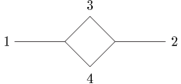
Figure 1: A diagrammatic representation of $\left<\phi_{2}\right|\delta V^{(2)}\left|\phi_{1}\right>$, a matrix element of the second-order change to the reduced interaction. The numbers label the particles.

Using the expression for $V^{(1)}$ in Eq. (36),

$$\left<\phi_{2}\right|\delta V^{(2)}\left|\phi_{1}\right> = \frac{1}{4}\int D_{3}D_{4}\,\delta_{2,34}\,\,\delta_{1,34}\,T_{2}^{(\Lambda,\Lambda^{\prime})}(F,K,I).\vspace{-.25in}$$ (54)

The integral over $p_{3}$ can be done with one of the delta functions. At this point it is convenient to change variables from $p_{4}^{+}$ and $\vec{p}_{4\perp}$ to $x$ and $\vec{r}_{\perp}$:

$$p_{4}=(p_{4}^{+},\vec{p}_{4\perp})=(xp_{1}^{+},x\vec{p}_{1\perp}+\vec{r}_{\perp}),\vspace{-.25in}$$ (55)

where $x$ is the fraction of the total longitudinal momentum carried by particle 4 and $\vec{r}_{\perp}$ is the transverse momentum of particle 4 in the center-of-mass frame. Since $p_{4}^{-}$ is constrained, we do not display it in the list of components of $p_{4}$. The momentum-conserving delta functions imply

$$p_{3}=\left([1-x]p_{1}^{+},[1-x]\vec{p}_{1\perp}-\vec{r}_{\perp}\right).\vspace{-.25in}$$ (56)

Note that all longitudinal momenta are positive, although we do not explicitly show these limits in integrals. This implies, for example, that $0<x<1$. With the change of variables, Eq. (54) becomes

$$\left<\phi_{2}\right|\delta V^{(2)}\left|\phi_{1}\right> = \frac{1}{4}p_{1}^{+}\delta^{(5)}(p_{2}-p_{1})\int d^{4}r_{\perp}dx\frac{1}{x(1-x)}T_{2}^{(\Lambda,\Lambda^{\prime})}(F,K,I).\vspace{-.25in}$$ (57)

We are using massless particles; so the free masses of the states $\left|I\right>=\left|\phi_{1}\right>$ and $\left|F\right>=\left|\phi_{2}\right>$ are zero:

$$M^{2}_{I}=M^{2}_{F}=0.\vspace{-.25in}$$ (58)

The particles in the intermediate state $\left|K\right>=\left|\phi_{3}\phi_{4}\right>$ are also massless, but the state still has a free mass from the particles’ relative motion:

$$M^{2}_{K}=\frac{\vec{r}^{\,2}_{\perp}}{x(1-x)}.\vspace{-.25in}$$ (59)

Then from the definition of the cutoff function $T_{2}^{(\Lambda,\Lambda^{\prime})}$,

$$T_{2}^{(\Lambda,\Lambda^{\prime})}(F,K,I)=-\frac{2x(1-x)}{\vec{r}^{\,2}_{\perp}}\left(e^{-2\Lambda^{\prime-4}\frac{\vec{r}^{\,4}_{\perp}}{x^{2}(1-x)^{2}}}-e^{-2\Lambda^{-4}\frac{\vec{r}^{\,4}_{\perp}}{x^{2}(1-x)^{2}}}\right).\vspace{-.25in}$$ (60)

After the integral is done, Eq. (57) becomes

$$\left<\phi_{2}\right|\delta V^{(2)}\left|\phi_{1}\right> = \,\delta_{1,2}\,\frac{1}{1536\pi^{3}}\sqrt{\frac{\pi}{2}}\left(\Lambda^{2}-\Lambda^{\prime 2}\right).\vspace{-.25in}$$ (61)

Applying Eq. (50) yields the matrix element of the second-order reduced interaction:

$$\left<\phi_{2}\right|V^{(2)}(\Lambda)\left|\phi_{1}\right> = \,\delta_{1,2}\,\Lambda^{2}\frac{1}{1536\pi^{3}}\sqrt{\frac{\pi}{2}}.\vspace{-.25in}$$ (62)

Using the definition of the Hamiltonian in terms of the reduced interaction, we find that to second-order, the matrix element of the Hamiltonian is given by

$$\left<\phi_{2}\right|{\cal M}^{2}(\Lambda)\left|\phi_{1}\right>=\,\delta_{1,2}\,\Lambda^{2}\;g_{{}_{\Lambda}}^{2}\frac{1}{1536\pi^{3}}\sqrt{\frac{\pi}{2}}.\vspace{-.25in}$$ (63)

This matrix element of the Hamiltonian has been completely determined to second-order, in terms of the fundamental parameters of the theory, by the restrictions that the Hamiltonian has to produce cutoff-independent physical quantities and has to respect the unviolated physical principles of the theory. If we wanted to compute physical quantities, this is one of the matrix elements of the Hamiltonian that we might need. We would have to choose $\Lambda$ and determine $g_{{}_{\Lambda}}$ by fitting data since the theory contains one adjustable parameter. Note that Eq. (63) is consistent with all the restrictions that we have placed on the Hamiltonian.

5.2 Example: $\left<\phi_{3}\phi_{4}\right|{\cal M}^{2}(\Lambda)\left|\phi_{1}\phi_{2}\right>$

Next we calculate the matrix element $\left<\phi_{3}\phi_{4}\right|{\cal M}^{2}(\Lambda)\left|\phi_{1}\phi_{2}\right>$ to ${\cal O}(g_{{}_{\Lambda}}^{2})$. We use $\left|I\right>=\left|\phi_{1}\phi_{2}\right>$ and $\left|F\right>=\left|\phi_{3}\phi_{4}\right>$. Then the matrix element of the second-order change to the reduced interaction is

$$\left<\phi_{3}\phi_{4}\right|\delta V^{(2)}\left|\phi_{1}\phi_{2}\right> = \frac{1}{2}\sum_{K}\left<\phi_{3}\phi_{4}\right|V^{(1)}\left|K\right>\left<K\right|V^{(1)}\left|\phi_{1}\phi_{2}\right>T_{2}^{(\Lambda,\Lambda^{\prime})}(F,K,I).\vspace{-.25in}$$ (64)

Since $V^{(1)}$ changes particle number by 1, $\left|K\right>$ has to be either a one- or three-particle state. When $V^{(1)}$ is substituted into the RHS of this equation and all the creation and annihilation operators from the possible intermediate states and the interactions are contracted, we see that $\left<\phi_{3}\phi_{4}\right|\delta V^{(2)}\left|\phi_{1}\phi_{2}\right>$ has contributions from a number of different processes. We define $\left<\phi_{3}\phi_{4}\right|\delta V^{(2)}\left|\phi_{1}\phi_{2}\right>_{i}$ to be the contribution to $\left<\phi_{3}\phi_{4}\right|\delta V^{(2)}\left|\phi_{1}\phi_{2}\right>$ from the process shown in Fig. 2-i, where $1\leq i\leq 9$.

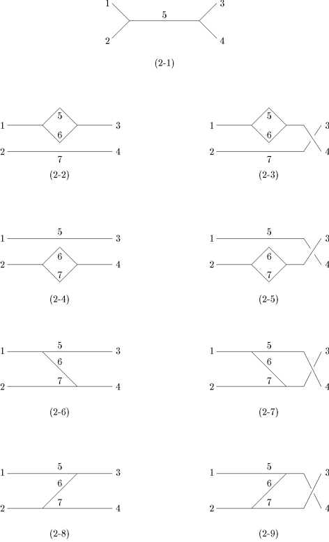
Figure 2: A diagrammatic representation of the contributions to $\left<\phi_{3}\phi_{4}\right|\delta V^{(2)}\left|\phi_{1}\phi_{2}\right>$, a matrix element of the second-order change to the reduced interaction. The numbers label the particles.

Then

$$\left<\phi_{3}\phi_{4}\right|\delta V^{(2)}\left|\phi_{1}\phi_{2}\right>=\sum_{i=1}^{9}\left<\phi_{3}\phi_{4}\right|\delta V^{(2)}\left|\phi_{1}\phi_{2}\right>_{i}.\vspace{-.25in}$$ (65)

Eq. (50) suggests that we define a contribution to the matrix element of the second-order reduced interaction for each contribution to $\left<\phi_{3}\phi_{4}\right|\delta V^{(2)}\left|\phi_{1}\phi_{2}\right>$:

$$\left<\phi_{3}\phi_{4}\right|V^{(2)}(\Lambda)\left|\phi_{1}\phi_{2}\right>_{i} = \left<\phi_{3}\phi_{4}\right|\delta V^{(2)}\left|\phi_{1}\phi_{2}\right>_{i}\>\rule[-11.38109pt]{0.28453pt}{22.76219pt}_{\;\Lambda\;\mathrm{terms}},\vspace{-.25in}$$ (66)

and then

$$\left<\phi_{3}\phi_{4}\right|V^{(2)}(\Lambda)\left|\phi_{1}\phi_{2}\right> = \sum_{i=1}^{9}\left<\phi_{3}\phi_{4}\right|V^{(2)}(\Lambda)\left|\phi_{1}\phi_{2}\right>_{i}.\vspace{-.25in}$$ (67)

For each contribution to $\left<\phi_{3}\phi_{4}\right|\delta V^{(2)}\left|\phi_{1}\phi_{2}\right>$, we use the change of variables

$$p_{1} = (xP^{+},x\vec{P}_{\perp}+\vec{r}_{\perp}),$$

$$p_{2} = ([1-x]P^{+},[1-x]\vec{P}_{\perp}-\vec{r}_{\perp}),$$

$$p_{3} = (yP^{+},y\vec{P}_{\perp}+\vec{q}_{\perp}),$$

$$p_{4} = ([1-y]P^{+},[1-y]\vec{P}_{\perp}-\vec{q}_{\perp}),\vspace{-.25in}$$ (68)

where $P=p_{1}+p_{2}$. Then the initial and final free masses are

$$M_{I}^{2} = \frac{\vec{r}^{\,2}_{\perp}}{x(1-x)},$$

$$M_{F}^{2} = \frac{\vec{q}^{\,2}_{\perp}}{y(1-y)}.$$

5.2.1 The Annihilation Contribution

The contribution to $\left<\phi_{3}\phi_{4}\right|\delta V^{(2)}\left|\phi_{1}\phi_{2}\right>$ from the annihilation process, shown in Fig. 2-1, is

$$\left<\phi_{3}\phi_{4}\right|\delta V^{(2)}\left|\phi_{1}\phi_{2}\right>_{1} = \frac{1}{2}\int D_{5}\left<\phi_{3}\phi_{4}\right|V^{(1)}\left|\phi_{5}\right>\left<\phi_{5}\right|V^{(1)}\left|\phi_{1}\phi_{2}\right>T_{2}^{(\Lambda,\Lambda^{\prime})}(F,K,I)$$ (70)

$$= \,\delta_{12,34}\,\frac{1}{2}\left(\frac{1}{M_{F}^{2}}+\frac{1}{M_{I}^{2}}\right)\left(e^{-2\Lambda^{\prime-4}M_{F}^{2}M_{I}^{2}}-e^{-2\Lambda^{-4}M_{F}^{2}M_{I}^{2}}\right),\vspace{-.25in}$$

where the intermediate state is $\left|K\right>=\left|\phi_{5}\right>$. According to Eq. (66), the corresponding part of the matrix element of the second-order reduced interaction is

$$\left<\phi_{3}\phi_{4}\right|V^{(2)}(\Lambda)\left|\phi_{1}\phi_{2}\right>_{1} = \,\delta_{12,34}\,\frac{1}{2}\left(\frac{1}{M_{F}^{2}}+\frac{1}{M_{I}^{2}}\right)\left(e^{-2\Lambda^{\prime-4}M_{F}^{2}M_{I}^{2}}-e^{-2\Lambda^{-4}M_{F}^{2}M_{I}^{2}}\right)\>\rule[-11.38109pt]{0.28453pt}{22.76219pt}_{\;\Lambda\;\mathrm{terms}}.\vspace{-.25in}$$ (71)

If we expand everything multiplying the delta function in powers of transverse momenta, the lowest order terms from the two exponentials cancel and leave two types of terms: those depending on $\Lambda$ and those depending on $\Lambda^{\prime}$. We can remove the $\Lambda^{\prime}$-dependent terms without altering the cancellation of the lowest term by replacing the first exponential with a $1$:

$$\left<\phi_{3}\phi_{4}\right|V^{(2)}(\Lambda)\left|\phi_{1}\phi_{2}\right>_{1} = \,\delta_{12,34}\,\frac{1}{2}\left(\frac{1}{M_{F}^{2}}+\frac{1}{M_{I}^{2}}\right)\left(1-e^{-2\Lambda^{-4}M_{F}^{2}M_{I}^{2}}\right).\vspace{-.25in}$$ (72)

5.2.2 The Two-Particle Self-Energy Contributions

The rest of the contributions to $\left<\phi_{3}\phi_{4}\right|\delta V^{(2)}\left|\phi_{1}\phi_{2}\right>$ have a three-body intermediate state, $\left|K\right>=\left|\phi_{5}\phi_{6}\phi_{7}\right>$. The contribution from the two-particle self-energy, shown in Fig. 2-2, is given by

$$\left<\phi_{3}\phi_{4}\right|\delta V^{(2)}\left|\phi_{1}\phi_{2}\right>_{2} = \frac{1}{4}\frac{1}{xy}\int D_{5}\,D_{6}\,D_{7}\,T_{2}^{(\Lambda,\Lambda^{\prime})}(F,K,I)\,\delta_{3,56}\,\,\delta_{7,4}\,\,\delta_{1,65}\,\,\delta_{7,2}\,.\vspace{-.25in}$$ (73)

We use the change of variables

$$p_{5} = (zp_{1}^{+},z\vec{p}_{1\perp}+\vec{k}_{\perp}),\vspace{-.25in}$$ (74)

and do the integrals over $p_{6}$ and $p_{7}$ using the delta functions. Then we find that

$$p_{6} = ([1-z]p_{1}^{+},[1-z]\vec{p}_{1\perp}-\vec{k}_{\perp}),\vspace{-.25in}$$ (75)

and the free mass of the intermediate state is

$$M_{K}^{2} = \frac{\vec{r}^{\,2}_{\perp}}{x(1-x)}+\frac{\vec{k}^{\,2}_{\perp}}{z(1-z)x},\vspace{-.25in}$$ (76)

and

$$\left<\phi_{3}\phi_{4}\right|\delta V^{(2)}\left|\phi_{1}\phi_{2}\right>_{2} = \frac{1}{2}\frac{1}{64\pi^{5}}\,\delta_{1,3}\,\,\delta_{2,4}\,\frac{1}{x}\int d^{4}k_{\perp}dz\frac{1}{\vec{k}^{\,2}_{\perp}}\left[e^{-2\Lambda^{-4}\Delta^{2}_{IK}}-e^{-2\Lambda^{\prime-4}\Delta^{2}_{IK}}\right]$$ (77)

$$= \,\delta_{1,3}\,\,\delta_{2,4}\,\frac{1}{1536\pi^{3}}\sqrt{\frac{\pi}{2}}\left(\Lambda^{2}-\Lambda^{\prime 2}\right).\vspace{-.25in}$$

According to Eq. (66), the corresponding part of the matrix element of the second-order reduced interaction is

$$\left<\phi_{3}\phi_{4}\right|V^{(2)}(\Lambda)\left|\phi_{1}\phi_{2}\right>_{2} = \,\delta_{1,3}\,\,\delta_{2,4}\,\Lambda^{2}\frac{1}{1536\pi^{3}}\sqrt{\frac{\pi}{2}}.\vspace{-.25in}$$ (78)

Note that Eqs. (62) and (78) indicate that to ${\cal O}(g_{{}_{\Lambda}}^{2})$ in this theory the only effect a spectator has on the self-energy is to produce an extra delta function. This is what one would expect if cluster decomposition were maintained. However, there is no guarantee that this will hold to all orders, and it is known that in gauge theories $\left<\phi_{3}\phi_{4}\right|V^{(2)}(\Lambda)\left|\phi_{1}\phi_{2}\right>_{2}$ depends on $p_{2}^{+}/P^{+}$. This is allowed because our cutoff partially violates cluster decomposition.

According to Fig. 2,

$$\left<\phi_{3}\phi_{4}\right|V^{(2)}(\Lambda)\left|\phi_{1}\phi_{2}\right>_{3} = \left<\phi_{3}\phi_{4}\right|V^{(2)}(\Lambda)\left|\phi_{1}\phi_{2}\right>_{2}\>\rule[-11.38109pt]{0.28453pt}{22.76219pt}_{\;3\leftrightarrow 4}=\,\delta_{1,4}\,\,\delta_{2,3}\,\Lambda^{2}\frac{1}{1536\pi^{3}}\sqrt{\frac{\pi}{2}},$$

$$\left<\phi_{3}\phi_{4}\right|V^{(2)}(\Lambda)\left|\phi_{1}\phi_{2}\right>_{4} = \left<\phi_{3}\phi_{4}\right|V^{(2)}(\Lambda)\left|\phi_{1}\phi_{2}\right>_{2}\>\rule[-11.38109pt]{0.28453pt}{22.76219pt}_{\;3\leftrightarrow 4}^{\;1\leftrightarrow 2}=\,\delta_{1,3}\,\,\delta_{2,4}\,\Lambda^{2}\frac{1}{1536\pi^{3}}\sqrt{\frac{\pi}{2}},$$

$$\left<\phi_{3}\phi_{4}\right|V^{(2)}(\Lambda)\left|\phi_{1}\phi_{2}\right>_{5} = \left<\phi_{3}\phi_{4}\right|V^{(2)}(\Lambda)\left|\phi_{1}\phi_{2}\right>_{4}\>\rule[-11.38109pt]{0.28453pt}{22.76219pt}_{\;3\leftrightarrow 4}=\,\delta_{1,4}\,\,\delta_{2,3}\,\Lambda^{2}\frac{1}{1536\pi^{3}}\sqrt{\frac{\pi}{2}}.\vspace{-.25in}$$ (79)

5.2.3 The Exchange Contributions

The exchange contribution to the matrix element of the second-order change in the reduced interaction, shown in Fig. 2-6, is

$$\left<\phi_{3}\phi_{4}\right|\delta V^{(2)}\left|\phi_{1}\phi_{2}\right>_{6} = \frac{1}{2}\frac{1}{x(1-y)}\int D_{5}D_{6}D_{7}T_{2}^{(\Lambda,\Lambda^{\prime})}(F,K,I)\,\delta_{4,67}\,\,\delta_{7,2}\,\,\delta_{1,56}\,\,\delta_{5,3}\,$$ (80)

$$= -\,\delta_{12,34}\,\frac{1}{2}\frac{1}{x-y}\left[\frac{1}{\Delta_{KF}}+\frac{1}{\Delta_{KI}}\right]\left[e^{-2\Lambda^{\prime-4}\Delta_{KF}\Delta_{KI}}-e^{-2\Lambda^{-4}\Delta_{KF}\Delta_{KI}}\right],\vspace{-.25in}$$

where the free mass of the intermediate state is

$$M_{K}^{2} = \frac{\vec{r}^{\,2}_{\perp}}{1-x}+\frac{\vec{q}^{\,2}_{\perp}}{y}+\frac{(\vec{r}_{\perp}-\vec{q}_{\perp})^{2}}{x-y}.\vspace{-.25in}$$ (81)

Eq. (66) implies that the corresponding part of the matrix element of the second-order reduced interaction is given by

$$\left<\phi_{3}\phi_{4}\right|V^{(2)}(\Lambda)\left|\phi_{1}\phi_{2}\right>_{6}=-\,\delta_{12,34}\,\frac{1}{2}\frac{1}{x-y}\left[\frac{1}{\Delta_{KF}}+\frac{1}{\Delta_{KI}}\right]\left[1-e^{-2\Lambda^{-4}\Delta_{KF}\Delta_{KI}}\right].\vspace{-.25in}$$ (82)

According to Fig. 2, the remaining parts of the matrix element of the second-order reduced interaction are given by

$$\left<\phi_{3}\phi_{4}\right|V^{(2)}(\Lambda)\left|\phi_{1}\phi_{2}\right>_{7} = \left<\phi_{3}\phi_{4}\right|V^{(2)}(\Lambda)\left|\phi_{1}\phi_{2}\right>_{6}\>\rule[-11.38109pt]{0.28453pt}{22.76219pt}_{\;3\leftrightarrow 4}=\left<\phi_{3}\phi_{4}\right|V^{(2)}(\Lambda)\left|\phi_{1}\phi_{2}\right>_{6}\>\rule[-11.38109pt]{0.28453pt}{22.76219pt}_{\;y\rightarrow 1-y\,,\,\vec{q}_{\perp}\rightarrow-\vec{q}_{\perp}},$$

$$\left<\phi_{3}\phi_{4}\right|V^{(2)}(\Lambda)\left|\phi_{1}\phi_{2}\right>_{8} = \left<\phi_{3}\phi_{4}\right|V^{(2)}(\Lambda)\left|\phi_{1}\phi_{2}\right>_{6}\>\rule[-11.38109pt]{0.28453pt}{22.76219pt}_{\;3\leftrightarrow 4}^{\;1\leftrightarrow 2}=\left<\phi_{3}\phi_{4}\right|V^{(2)}(\Lambda)\left|\phi_{1}\phi_{2}\right>_{6}\>\rule[-11.38109pt]{0.28453pt}{22.76219pt}_{\;y\rightarrow 1-y\,,\,\vec{q}_{\perp}\rightarrow-\vec{q}_{\perp}}^{\;x\rightarrow 1-x\,,\,\vec{r}_{\perp}\rightarrow-\vec{r}_{\perp}},$$

$$\left<\phi_{3}\phi_{4}\right|V^{(2)}(\Lambda)\left|\phi_{1}\phi_{2}\right>_{9} = \left<\phi_{3}\phi_{4}\right|V^{(2)}(\Lambda)\left|\phi_{1}\phi_{2}\right>_{8}\>\rule[-11.38109pt]{0.28453pt}{22.76219pt}_{\;3\leftrightarrow 4}=\left<\phi_{3}\phi_{4}\right|V^{(2)}(\Lambda)\left|\phi_{1}\phi_{2}\right>_{6}\>\rule[-11.38109pt]{0.28453pt}{22.76219pt}_{\;x\rightarrow 1-x\,,\,\vec{r}_{\perp}\rightarrow-\vec{r}_{\perp}}.\vspace{-.25in}$$ (83)

5.2.4 The Complete Matrix Element and Transverse Locality

Using Eqs. (6) and (33), we can write the full second-order matrix element of the Hamiltonian:

$$\left<\phi_{3}\phi_{4}\right|{\cal M}^{2}(\Lambda)\left|\phi_{1}\phi_{2}\right> = (\,\delta_{1,3}\,\,\delta_{2,4}\,+\,\delta_{1,4}\,\,\delta_{2,3}\,)M_{F}^{2}+e^{-\Lambda^{-4}\Delta^{2}_{FI}}g_{{}_{\Lambda}}^{2}\sum_{i=1}^{9}\left<\phi_{3}\phi_{4}\right|V^{(2)}(\Lambda)\left|\phi_{1}\phi_{2}\right>_{i}.\vspace{-.25in}$$ (84)

By inspection, it is clear that this result respects all the restrictions we have placed on the Hamiltonian, except perhaps the requirement that it can be represented as a power series in transverse momenta with an infinite radius of convergence. To see how to check this, consider the first term in the sum on the RHS:

$$e^{-\Lambda^{-4}\Delta^{2}_{FI}}g_{{}_{\Lambda}}^{2}\left<\phi_{3}\phi_{4}\right|V^{(2)}(\Lambda)\left|\phi_{1}\phi_{2}\right>_{1} = \,\delta_{12,34}\,\frac{1}{2}g_{{}_{\Lambda}}^{2}e^{-\Lambda^{-4}\left(M_{F}^{2}-M_{I}^{2}\right)^{2}}\left(\frac{1}{M_{F}^{2}}+\frac{1}{M_{I}^{2}}\right)$$ (85)

$$\times \left(1-e^{-2\Lambda^{-4}M_{F}^{2}M_{I}^{2}}\right).\vspace{-.25in}$$

The presence of the mass denominators might seem likely to cause a problem with the convergence of a power series expansion. Everything multiplying the delta function can be expressed as a power series in transverse momenta if it can be expressed as a power series in $M_{F}^{2}$ and $M_{I}^{2}$, since it is a function only of these and since $M_{F}^{2}$ and $M_{I}^{2}$ are themselves power series in transverse momenta. We can write

$$e^{-\Lambda^{-4}\Delta^{2}_{FI}}g_{{}_{\Lambda}}^{2}\left<\phi_{3}\phi_{4}\right|V^{(2)}(\Lambda)\left|\phi_{1}\phi_{2}\right>_{1}=\,\delta_{12,34}\,\frac{1}{2}g_{{}_{\Lambda}}^{2}\frac{1}{\Lambda^{2}}\bigg{[}\frac{2}{\Lambda^{2}}(M_{F}^{2}+M_{I}^{2})-\frac{2}{\Lambda^{6}}(M_{F}^{6}+M_{I}^{6})$$ (86)

$$+ \frac{1}{\Lambda^{10}}\left\{\frac{4}{3}(M_{F}^{4}M_{I}^{6}+M_{F}^{6}M_{I}^{4})-(M_{F}^{8}M_{I}^{2}+M_{F}^{2}M_{I}^{8})\right\}+\cdots\bigg{]}.\vspace{-.25in}$$

If we approximate the RHS of this equation by keeping only $N$ terms, the difference between this finite sum and the RHS of Eq. (85) can be made arbitrarily small, for any values of $M_{F}^{2}$ and $M_{I}^{2}$, by making $N$ large enough. This means that $e^{-\Lambda^{-4}\Delta^{2}_{FI}}g_{{}_{\Lambda}}^{2}\left<\phi_{3}\phi_{4}\right|V^{(2)}(\Lambda)\left|\phi_{1}\phi_{2}\right>_{1}$ can indeed be represented as a power series in transverse momenta with an infinite radius of convergence. The other contributions to $\left<\phi_{3}\phi_{4}\right|{\cal M}^{2}(\Lambda)\left|\phi_{1}\phi_{2}\right>$ can be analyzed similarly, and the conclusion is the same for each.

5.3 Example: $\left<\phi_{2}\phi_{3}\phi_{4}\right|{\cal M}^{2}(\Lambda)\left|\phi_{1}\right>$

The final second-order matrix element of the Hamiltonian that we calculate is $\left<\phi_{2}\phi_{3}\phi_{4}\right|{\cal M}^{2}(\Lambda)\left|\phi_{1}\right>$. To compute this matrix element, we use $\left|I\right>=\left|\phi_{1}\right>$ and $\left|F\right>=\left|\phi_{2}\phi_{3}\phi_{4}\right>$. The matrix element of the second-order change to the reduced interaction is

$$\left<\phi_{2}\phi_{3}\phi_{4}\right|\delta V^{(2)}\left|\phi_{1}\right> = \frac{1}{2}\sum_{K}\left<\phi_{2}\phi_{3}\phi_{4}\right|V^{(1)}\left|K\right>\left<K\right|V^{(1)}\left|\phi_{1}\right>T_{2}^{(\Lambda,\Lambda^{\prime})}(F,K,I).\vspace{-.25in}$$ (87)

Since $V^{(1)}$ changes particle number by 1, $\left|K\right>$ has to be a two-particle state.

We define $\left<\phi_{2}\phi_{3}\phi_{4}\right|\delta V^{(2)}\left|\phi_{1}\right>_{i}$ to be the contribution to $\left<\phi_{2}\phi_{3}\phi_{4}\right|\delta V^{(2)}\left|\phi_{1}\right>$ from the process shown in Fig. 3-i, where $1\leq i\leq 3$.

Figure 3: A diagrammatic representation of the contributions to $\left<\phi_{2}\phi_{3}\phi_{4}\right|\delta V^{(2)}\left|\phi_{1}\right>$, a matrix element of the second-order change to the reduced interaction. The numbers label the particles.

Then

$$\left<\phi_{2}\phi_{3}\phi_{4}\right|\delta V^{(2)}\left|\phi_{1}\right>=\sum_{i=1}^{3}\left<\phi_{2}\phi_{3}\phi_{4}\right|\delta V^{(2)}\left|\phi_{1}\right>_{i}.\vspace{-.25in}$$ (88)

Eq. (50) suggests that we define a contribution to the matrix element of the second-order reduced interaction for each contribution to $\left<\phi_{2}\phi_{3}\phi_{4}\right|\delta V^{(2)}\left|\phi_{1}\right>$:

$$\left<\phi_{2}\phi_{3}\phi_{4}\right|V^{(2)}(\Lambda)\left|\phi_{1}\right>_{i} = \left<\phi_{2}\phi_{3}\phi_{4}\right|\delta V^{(2)}\left|\phi_{1}\right>_{i}\>\rule[-11.38109pt]{0.28453pt}{22.76219pt}_{\;\Lambda\;\mathrm{terms}},\vspace{-.25in}$$ (89)

and then

$$\left<\phi_{2}\phi_{3}\phi_{4}\right|V^{(2)}(\Lambda)\left|\phi_{1}\right> = \sum_{i=1}^{3}\left<\phi_{2}\phi_{3}\phi_{4}\right|V^{(2)}(\Lambda)\left|\phi_{1}\right>_{i}.\vspace{-.25in}$$ (90)

For each contribution to $\left<\phi_{2}\phi_{3}\phi_{4}\right|\delta V^{(2)}\left|\phi_{1}\right>$, we use $\left|K\right>=\left|\phi_{5}\phi_{6}\right>$ and the change of variables

$$p_{2} = (xp_{1}^{+},x\vec{p}_{1\perp}+\vec{r}_{\perp}),$$

$$p_{3} = (yp_{1}^{+},y\vec{p}_{1\perp}+\vec{q}_{\perp}),$$

$$p_{4} = (zp_{1}^{+},z\vec{p}_{1\perp}+\vec{w}_{\perp}),\vspace{-.25in}$$ (91)

where

$$x+y+z = 1,$$

$$\vec{r}_{\perp}+\vec{q}_{\perp}+\vec{w}_{\perp} = 0.\vspace{-.25in}$$ (92)

Then the relevant differences of free masses are

$$\Delta_{FK} = \frac{\vec{r}^{\,2}_{\perp}}{x}+\frac{\vec{q}^{\,2}_{\perp}}{y}-\frac{\vec{w}^{\,2}_{\perp}}{x+y},$$

$$\Delta_{KI} = \vec{w}^{\,2}_{\perp}\left(\frac{1}{x+y}+\frac{1}{z}\right),$$

$$\Delta_{FI} = \frac{\vec{r}^{\,2}_{\perp}}{x}+\frac{\vec{q}^{\,2}_{\perp}}{y}+\frac{\vec{w}^{\,2}_{\perp}}{z},$$

and the contribution to the matrix element of the second-order change to the reduced interaction shown in Fig. 3-1 is

$$\left<\phi_{2}\phi_{3}\phi_{4}\right|\delta V^{(2)}\left|\phi_{1}\right>_{1} = \,\delta_{1,234}\,\frac{1}{2}\frac{1}{x+y}\left(\frac{1}{\Delta_{FK}}-\frac{1}{\Delta_{KI}}\right)\left(e^{2\Lambda^{\prime-4}\Delta_{FK}\Delta_{KI}}-e^{2\Lambda^{-4}\Delta_{FK}\Delta_{KI}}\right),\vspace{-.25in}$$ (94)

and the corresponding contribution to the matrix element of the second-order reduced interaction is

$$\left<\phi_{2}\phi_{3}\phi_{4}\right|V^{(2)}(\Lambda)\left|\phi_{1}\right>_{1} = \,\delta_{1,234}\,\frac{1}{2}\frac{1}{x+y}\left(\frac{1}{\Delta_{FK}}-\frac{1}{\Delta_{KI}}\right)$$ (95)

$$\times \left(e^{2\Lambda^{\prime-4}\Delta_{FK}\Delta_{KI}}-e^{2\Lambda^{-4}\Delta_{FK}\Delta_{KI}}\right)\>\rule[-11.38109pt]{0.28453pt}{22.76219pt}_{\;\Lambda\;\mathrm{terms}}.\vspace{-.25in}$$

As before, if we expand everything multiplying the delta function in powers of transverse momenta, the lowest order terms from the two exponentials cancel and leave two types of terms: those depending on $\Lambda$ and those depending on $\Lambda^{\prime}$. We can remove the $\Lambda^{\prime}$-dependent terms without altering the cancellation of the lowest term by replacing the first exponential with a $1$:

$$\left<\phi_{2}\phi_{3}\phi_{4}\right|V^{(2)}(\Lambda)\left|\phi_{1}\right>_{1} = \,\delta_{1,234}\,\frac{1}{2}\frac{1}{x+y}\left(\frac{1}{\Delta_{FK}}-\frac{1}{\Delta_{KI}}\right)\left(1-e^{2\Lambda^{-4}\Delta_{FK}\Delta_{KI}}\right).\vspace{-.25in}$$ (96)

According to Fig. 3, the other parts of the matrix element of the second-order reduced interaction are given by

$$\left<\phi_{2}\phi_{3}\phi_{4}\right|V^{(2)}(\Lambda)\left|\phi_{1}\right>_{2} = \left<\phi_{2}\phi_{3}\phi_{4}\right|V^{(2)}(\Lambda)\left|\phi_{1}\right>_{1}\>\rule[-11.38109pt]{0.28453pt}{22.76219pt}_{\;3\leftrightarrow 4}=\left<\phi_{2}\phi_{3}\phi_{4}\right|V^{(2)}(\Lambda)\left|\phi_{1}\right>_{1}\>\rule[-11.38109pt]{0.28453pt}{22.76219pt}_{\;y\leftrightarrow z\;,\;\vec{q}_{\perp}\leftrightarrow\vec{w}_{\perp}},\vspace{-.25in}$$ (97)

and

$$\left<\phi_{2}\phi_{3}\phi_{4}\right|V^{(2)}(\Lambda)\left|\phi_{1}\right>_{3} = \left<\phi_{2}\phi_{3}\phi_{4}\right|V^{(2)}(\Lambda)\left|\phi_{1}\right>_{1}\>\rule[-11.38109pt]{0.28453pt}{22.76219pt}_{\;2\rightarrow 3\;,\;3\rightarrow 4\;,\;4\rightarrow 2}$$ (98)

$$= \left<\phi_{2}\phi_{3}\phi_{4}\right|V^{(2)}(\Lambda)\left|\phi_{1}\right>_{1}\>\rule[-11.38109pt]{0.28453pt}{22.76219pt}^{\;x\rightarrow y\;,\;y\rightarrow z\;,\;z\rightarrow x}_{\;\vec{r}_{\perp}\rightarrow\vec{q}_{\perp}\;,\;\vec{q}_{\perp}\rightarrow\vec{w}_{\perp}\;,\;\vec{w}_{\perp}\rightarrow\vec{r}_{\perp}}.\vspace{-.25in}$$

Using the definition of the Hamiltonian in terms of the reduced interaction, we can write the full second-order matrix element of the Hamiltonian:

$$\left<\phi_{2}\phi_{3}\phi_{4}\right|{\cal M}^{2}(\Lambda)\left|\phi_{1}\right> = e^{-\Lambda^{-4}M_{F}^{4}}g_{{}_{\Lambda}}^{2}\sum_{i=1}^{3}\left<\phi_{2}\phi_{3}\phi_{4}\right|V^{(2)}(\Lambda)\left|\phi_{1}\right>_{i}.\vspace{-.25in}$$ (99)

This result is consistent with the restrictions we have placed on the Hamiltonian.

6 The Removal of Cutoff Dependence from Physical Quantities

One of the restrictions on the Hamiltonian is that it has to produce cutoff-independent physical quantities. To see how this requirement is fulfilled, consider as an example the scattering cross section for $\phi_{1}\phi_{2}\rightarrow\phi_{3}\phi_{4}$. At second order, the $T$ matrix has contributions from the $s$, $t$, and $u$ channels. The different channels are linearly independent functions of the external momenta; so each contribution should individually have all the properties required of the full $T$ matrix. For simplicity, we limit ourselves to consideration of the $s$ (annihilation) channel.

In our approach, the scattering matrix $S$ is defined by

$$\left<F\right|S\left|I\right>=\left<F\right|\left.\!I\right>-2\pi i\delta(P_{F}^{-}-P_{I}^{-})\left<F\right|T(P_{I}^{-})\left|I\right>,\vspace{-.25in}$$ (100)

where the $T$ matrix is defined by [16]

$$T(p^{-})=H_{I}(\Lambda)+H_{I}(\Lambda)\frac{1}{p^{-}-h+i\epsilon}T(p^{-}),\vspace{-.25in}$$ (101)

and $H_{I}(\Lambda)$ is the interacting part of the Hamiltonian cut off by $\Lambda$:

$$H_{I}(\Lambda)=\frac{{\cal M}^{2}_{I}(\Lambda)}{{\cal P}^{+}}.\vspace{-.25in}$$ (102)

To second order,

$$\left<\phi_{3}\phi_{4}\right|T(p_{1}^{-}+p_{2}^{-})\left|\phi_{1}\phi_{2}\right> = \left<\phi_{3}\phi_{4}\right|H_{I}(\Lambda)+H_{I}(\Lambda)\frac{1}{p_{1}^{-}+p_{2}^{-}-h+i\epsilon}H_{I}(\Lambda)\left|\phi_{1}\phi_{2}\right>.\vspace{-.25in}$$ (103)

If we neglect all noncanonical operators, the first term does not contribute and the second term can be calculated by inserting a complete set of free states. This leads to

$$\delta(P_{F}^{-}-P_{I}^{-})\left<\phi_{3}\phi_{4}\right|T(P_{I}^{-})\left|\phi_{1}\phi_{2}\right>=\frac{g_{{}_{\Lambda}}^{2}}{s}e^{-2\Lambda^{-4}s^{2}}64\pi^{5}\delta^{(6)}(p_{1}+p_{2}-p_{3}-p_{4}),\vspace{-.25in}$$ (104)

where $\left|I\right>=\left|\phi_{1}\phi_{2}\right>$, $\left|F\right>=\left|\phi_{3}\phi_{4}\right>$, and $s$ is the invariant mass-squared of $\left|\phi_{1}\phi_{2}\right>$. The cross section is cutoff-independent only if the $T$ matrix is cutoff-independent. Thus Eq. (104) shows that the cutoff appears in physical quantities if noncanonical operators are neglected. If we were to use an infinite cutoff, then the ${\cal O}(g_{{}_{\Lambda}}^{2})$ contribution to the cross section would be cutoff-independent but higher-order contributions would be infinite.

To test whether our procedure for computing ${\cal M}^{2}(\Lambda)$ leads to cutoff-independent physical quantities, we now include noncanonical operators. This means that we have to include the first term in Eq. (103):

$$\left<\phi_{3}\phi_{4}\right|H_{I}(\Lambda)\left|\phi_{1}\phi_{2}\right> = \frac{1}{p_{1}^{+}+p_{2}^{+}}e^{-\Lambda^{-4}\Delta^{2}_{FI}}g_{{}_{\Lambda}}^{2}\left<\phi_{3}\phi_{4}\right|V^{(2)}(\Lambda)\left|\phi_{1}\phi_{2}\right>_{1}$$ (105)

$$= \frac{g_{{}_{\Lambda}}^{2}}{s}\left(1-e^{-2\Lambda^{-4}s^{2}}\right)64\pi^{5}\delta^{(5)}(p_{1}+p_{2}-p_{3}-p_{4}),\vspace{-.25in}$$

where the result for the annihilation contribution to the second-order reduced interaction is used, and we use the fact that we only need the on-energy-shell part. This contribution shifts the $T$ matrix so that the total $T$ matrix is

$$\delta(P_{F}^{-}-P_{I}^{-})\left<\phi_{3}\phi_{4}\right|T(P_{I}^{-})\left|\phi_{1}\phi_{2}\right>=\frac{g_{{}_{\Lambda}}^{2}}{s}64\pi^{5}\delta^{(6)}(p_{1}+p_{2}-p_{3}-p_{4}).\vspace{-.25in}$$ (106)

Since $g_{{}_{\Lambda}}^{2}$ is cutoff-independent at second-order [$dg_{{}_{\Lambda}}^{2}/d\Lambda={\cal O}(g_{{}_{\Lambda}}^{4})$], this is the correct cutoff-independent result to ${\cal O}(g_{{}_{\Lambda}}^{2})$.

Our restrictions on the Hamiltonian have led to its matrix elements being such that they compensate for the presence of the cutoff in physical quantities. No proof exists, but we expect that our procedure leads to a renormalized Hamiltonian that produces exactly correct perturbative scattering amplitudes order-by-order. When this Hamiltonian is used nonperturbatively, however, there should be some cutoff dependence, as we have mentioned in previous sections.

7 $\left<\phi_{2}\phi_{3}\right|{\cal M}^{2}(\Lambda)\left|\phi_{1}\right>$ to Third Order

We wish to calculate $\left<\phi_{2}\phi_{3}\right|{\cal M}^{2}(\Lambda)\left|\phi_{1}\right>$ to third order to demonstrate how a higher-order calculation proceeds and to derive the running coupling in our approach. In Appendix D, we deduce that matrix elements of even-order reduced interactions cannot have contributions from three interacting particles. This means that $\left<\phi_{2}\phi_{3}\right|{\cal M}^{2}(\Lambda)\left|\phi_{1}\right>$ has only odd-order contributions. The first-order contribution is defined in terms of the first-order reduced interaction, which we have defined in Eq. (36). The third-order contribution is defined in terms of the third-order reduced interaction. In this section, we compute the third-order contribution, neglecting the cutoff-independent part of the third-order reduced interaction. Eq. (49) shows that a calculation of the cutoff-independent part would be a fifth-order calculation, which we prefer to avoid at this time.

According to Eq. (48), the cutoff-dependent part of the third-order reduced interaction is given by

$$\left<\phi_{2}\phi_{3}\right|V^{(3)}_{\mathrm{C\hskip 0.56905ptD}}(\Lambda)\left|\phi_{1}\right>=\left[\left<\phi_{2}\phi_{3}\right|\delta V^{(3)}\left|\phi_{1}\right>-B_{1,2}\left<\phi_{2}\phi_{3}\right|V^{(1)}\left|\phi_{1}\right>\right]_{\Lambda\;\mathrm{terms}}.\vspace{-.25in}$$ (107)

$\left<\phi_{2}\phi_{3}\right|\delta V^{(3)}\left|\phi_{1}\right>$ is defined by

$$\left<\phi_{2}\phi_{3}\right|\delta V^{(3)}\left|\phi_{1}\right> = \frac{1}{2}\sum_{K}\left<\phi_{2}\phi_{3}\right|V^{(1)}\left|K\right>\left<K\right|V^{(2)}(\Lambda^{\prime})\left|\phi_{1}\right>T_{2}^{(\Lambda,\Lambda^{\prime})}$$ (108)

$$+ \frac{1}{2}\sum_{K}\left<\phi_{2}\phi_{3}\right|V^{(2)}(\Lambda^{\prime})\left|K\right>\left<K\right|V^{(1)}\left|\phi_{1}\right>T_{2}^{(\Lambda,\Lambda^{\prime})}$$

$$+ \frac{1}{4}\sum_{K,L}\left<\phi_{2}\phi_{3}\right|V^{(1)}\left|K\right>\left<K\right|V^{(1)}\left|L\right>\left<L\right|V^{(1)}\left|\phi_{1}\right>T_{3}^{(\Lambda,\Lambda^{\prime})},\vspace{-.25in}$$

where we are suppressing the dependence of the cutoff functions on the states. Note that $B_{1,2}=C_{3}$ and is given by

$$B_{1,2} = C_{3}=\left[64\pi^{5}p_{1}^{+}\delta^{(5)}(p_{1}-p_{2}-p_{3})\right]^{-1}\left<\phi_{2}\phi_{3}\right|\delta V^{(3)}\left|\phi_{1}\right>\>\rule[-11.38109pt]{0.28453pt}{25.60747pt}_{\;\vec{p}_{2\perp}=\vec{p}_{3\perp}=0\,;\,p_{2}^{+}=p_{3}^{+}=\frac{1}{2}p_{1}^{+}}$$ (109)

$$= \left[\left<\phi_{2}\phi_{3}\right|V^{(1)}\left|\phi_{1}\right>\right]^{-1}\left<\phi_{2}\phi_{3}\right|\delta V^{(3)}\left|\phi_{1}\right>\>\rule[-11.38109pt]{0.28453pt}{25.60747pt}_{\;\vec{p}_{2\perp}=\vec{p}_{3\perp}=0\,;\,p_{2}^{+}=p_{3}^{+}=\frac{1}{2}p_{1}^{+}}.\vspace{-.25in}$$

Eq. (107) then becomes

$$\left<\phi_{2}\phi_{3}\right|V^{(3)}_{\mathrm{C\hskip 0.56905ptD}}(\Lambda)\left|\phi_{1}\right>=\left[\left<\phi_{2}\phi_{3}\right|\delta V^{(3)}\left|\phi_{1}\right>-\left<\phi_{2}\phi_{3}\right|\delta V^{(3)}\left|\phi_{1}\right>\>\rule[-11.38109pt]{0.28453pt}{25.60747pt}_{\;\vec{p}_{2\perp}=\vec{p}_{3\perp}=0\,;\,p_{2}^{+}=p_{3}^{+}=\frac{1}{2}p_{1}^{+}}\right]_{\Lambda\;\mathrm{terms}}.\vspace{-.25in}$$ (110)

This indicates that $\left<\phi_{2}\phi_{3}\right|V^{(3)}_{\mathrm{C\hskip 0.56905ptD}}(\Lambda)\left|\phi_{1}\right>$ can be computed solely in terms of $\left<\phi_{2}\phi_{3}\right|\delta V^{(3)}\left|\phi_{1}\right>$, which we now calculate.

All the matrix elements of the second-order reduced interaction that can appear on the RHS of Eq. (108) were calculated in the previous section. When $\left<\phi_{2}\phi_{3}\right|\delta V^{(3)}\left|\phi_{1}\right>$ is expanded in terms of the possible intermediate states and possible contributions to matrix elements of $V^{(1)}$ and $V^{(2)}(\Lambda^{\prime})$, we see that it has contributions from a number of different processes. We define $\left<\phi_{2}\phi_{3}\right|\delta V^{(3)}\left|\phi_{1}\right>_{i}$ to be the contribution to $\left<\phi_{2}\phi_{3}\right|\delta V^{(3)}\left|\phi_{1}\right>$ from the process shown in Fig. 4-i, where $1\leq i\leq 15$.

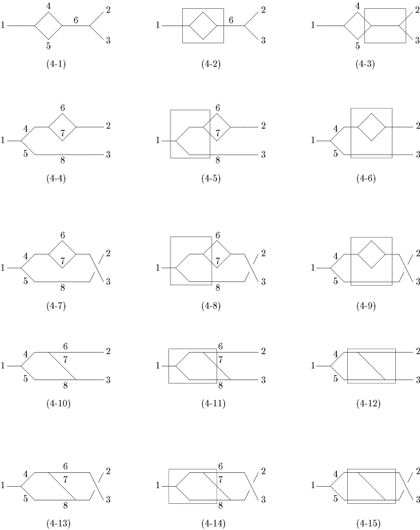
Figure 4: A diagrammatic representation of the contributions to $\left<\phi_{2}\phi_{3}\right|\delta V^{(3)}\left|\phi_{1}\right>$. The numbers label the particles, the bare vertices represent matrix elements of $V^{(1)}$, and the boxes represent contributions to matrix elements of $V^{(2)}(\Lambda^{\prime})$ corresponding to the processes depicted in the boxes.

In Fig. 4, the plain vertices represent matrix elements of $V^{(1)}$ and the boxes represent contributions to matrix elements of $V^{(2)}(\Lambda^{\prime})$ corresponding to the processes depicted in the boxes. For example, the box in Fig. 4-12 represents $\left<\phi_{2}\phi_{3}\right|V^{(2)}(\Lambda^{\prime})\left|\phi_{4}\phi_{5}\right>_{6}$ [see Fig. 2-6 and Eq. (82)]. Note that not every contribution to every matrix element of $V^{(2)}(\Lambda^{\prime})$ that appears in Eq. (108) appears in Fig 4. For example, $\left<\phi_{2}\phi_{3}\right|V^{(2)}(\Lambda^{\prime})\left|\phi_{4}\phi_{5}\right>_{9}$ [see Fig. 2-9 and Eq. (83)] does not appear in Fig. 4, because when it is paired with $\left<\phi_{4}\phi_{5}\right|V^{(1)}\left|\phi_{1}\right>$ and we integrate over $p_{4}$ and $p_{5}$, it gives an identical contribution to $\left<\phi_{2}\phi_{3}\right|V^{(2)}(\Lambda^{\prime})\left|\phi_{4}\phi_{5}\right>_{6}$. For this reason, $\left<\phi_{2}\phi_{3}\right|\delta V^{(3)}\left|\phi_{1}\right>_{12}$, shown in Fig. 4-12, includes contributions from both. Then $\left<\phi_{2}\phi_{3}\right|\delta V^{(3)}\left|\phi_{1}\right>$ is

$$\left<\phi_{2}\phi_{3}\right|\delta V^{(3)}\left|\phi_{1}\right>=\sum_{i=1}^{15}\left<\phi_{2}\phi_{3}\right|\delta V^{(3)}\left|\phi_{1}\right>_{i}.\vspace{-.25in}$$ (111)

For each contribution to $\left<\phi_{2}\phi_{3}\right|\delta V^{(3)}\left|\phi_{1}\right>$, we use the change of variables

$$p_{2} = (yp_{1}^{+},y\vec{p}_{1\perp}+\vec{q}_{\perp}),$$

$$p_{3} = ([1-y]p_{1}^{+},[1-y]\vec{p}_{1\perp}-\vec{q}_{\perp}),\vspace{-.25in}$$ (112)

which leads to the initial and final free masses

$$M_{I}^{2} = 0,$$

$$M_{F}^{2} = \frac{\vec{q}^{\,2}_{\perp}}{y(1-y)}.\vspace{-.25in}$$ (113)

7.1 The One-Particle Self-Energy Contributions

The contributions to the matrix element of the third-order change to the reduced interaction from one-particle self-energies, shown in Figs. 4-1, 4-2, and 4-3, can be combined because they have similar structures. For each of them we use

$$\left|L\right> = \left|\phi_{4}\phi_{5}\right>,$$

$$\left|K\right> = \left|\phi_{6}\right>,$$

and the change of variables

$$p_{4} = (xp_{1}^{+},x\vec{p}_{1\perp}+\vec{r}_{\perp}),$$

$$p_{5} = ([1-x]p_{1}^{+},[1-x]\vec{p}_{1\perp}-\vec{r}_{\perp}),\vspace{-.25in}$$ (115)

which leads to the intermediate free masses

$$M_{K}^{2} = 0,$$

$$M_{L}^{2} = \frac{\vec{r}^{\,2}_{\perp}}{x(1-x)},\vspace{-.25in}$$ (116)

and $p_{6}=p_{1}$. The contribution from Fig. 4-1 is

$$\left<\phi_{2}\phi_{3}\right|\delta V^{(3)}\left|\phi_{1}\right>_{1} = \frac{1}{8}\int D_{4}D_{5}D_{6}\left<\phi_{2}\phi_{3}\right|V^{(1)}\left|\phi_{6}\right>\left<\phi_{6}\right|V^{(1)}\left|\phi_{4}\phi_{5}\right>\left<\phi_{4}\phi_{5}\right|V^{(1)}\left|\phi_{1}\right>T_{3}^{(\Lambda,\Lambda^{\prime})}(F,K,L,I)$$ (117)

$$= \frac{N}{2\pi^{2}}\int d^{4}r_{\perp}dx\frac{1}{x(1-x)}T_{3}^{(\Lambda,\Lambda^{\prime})}(F,K,L,I),\vspace{-.25in}$$

where

$$N=\frac{\pi^{2}}{4}p_{1}^{+}\delta^{(5)}(p_{1}-p_{2}-p_{3}).\vspace{-.25in}$$ (118)

The contribution from Fig. 4-2 is

$$\left<\phi_{2}\phi_{3}\right|\delta V^{(3)}\left|\phi_{1}\right>_{2} = \frac{1}{2}\int D_{6}\left<\phi_{2}\phi_{3}\right|V^{(1)}\left|\phi_{6}\right>\left<\phi_{6}\right|V^{(2)}(\Lambda^{\prime})\left|\phi_{1}\right>T_{2}^{(\Lambda,\Lambda^{\prime})}(F,K,I)$$ (119)

$$= \frac{N}{12}\sqrt{\frac{\pi}{2}}\Lambda^{\prime 2}T_{2}^{(\Lambda,\Lambda^{\prime})}(F,K,I),\vspace{-.25in}$$

and the contribution from Fig. 4-3 is

$$\left<\phi_{2}\phi_{3}\right|\delta V^{(3)}\left|\phi_{1}\right>_{3}=\frac{1}{4}\int D_{4}D_{5}\left<\phi_{2}\phi_{3}\right|V^{(2)}(\Lambda^{\prime})\left|\phi_{4}\phi_{5}\right>_{1}\left<\phi_{4}\phi_{5}\right|V^{(1)}\left|\phi_{1}\right>T_{2}^{(\Lambda,\Lambda^{\prime})}(F,L,I)$$ (120)

$$= \frac{N}{2\pi^{2}}\int d^{4}r_{\perp}dx\frac{1}{x(1-x)}\left(\frac{1}{M_{L}^{2}}+\frac{1}{M_{F}^{2}}\right)\left(1-e^{-2\Lambda^{\prime-4}M_{L}^{2}M_{F}^{2}}\right)T_{2}^{(\Lambda,\Lambda^{\prime})}(F,L,I).\vspace{-.25in}$$

It is easiest to combine these three contributions before doing the integral in Eq. (117). This leads to

$$\sum_{i=1}^{3}\left<\phi_{2}\phi_{3}\right|\delta V^{(3)}\left|\phi_{1}\right>_{i} = \frac{N}{12}\int_{0}^{\infty}d(M_{L}^{2})\left\{e^{-2\Lambda^{\prime-4}M_{L}^{4}}\left[\frac{1}{M_{L}^{2}}+\frac{M_{F}^{2}}{M_{L}^{4}}+\frac{2}{M_{F}^{2}}\right.\right.$$ (121)

$$+ \left.\left.e^{2\Lambda^{\prime-4}M_{L}^{2}M_{F}^{2}}\left(\frac{1}{\Delta_{FL}}-\frac{1}{M_{L}^{2}}+\frac{M_{L}^{2}}{M_{F}^{2}\Delta_{FL}}-\frac{1}{M_{F}^{2}}\right)\right]-[\Lambda^{\prime}\rightarrow\Lambda]\right\}.\vspace{-.25in}$$

This one-dimensional integral cannot be done analytically for arbitrary $M_{F}^{2}$; so we consider it to be a function of $M_{F}^{2}$ that must be computed numerically.

7.2 The Two-Particle Self-Energy Contributions

The contributions to the matrix element of the third-order change to the reduced interaction from two-particle self-energies, shown in Figs. 4-4, 4-5, and 4-6, can be combined. For each of these we use

$$\left|L\right> = \left|\phi_{4}\phi_{5}\right>,$$

$$\left|K\right> = \left|\phi_{6}\phi_{7}\phi_{8}\right>,$$

and the change of variables

$$p_{6} = (xp_{2}^{+},x\vec{p}_{2\perp}+\vec{r}_{\perp}),$$

$$p_{7} = ([1-x]p_{2}^{+},[1-x]\vec{p}_{2\perp}-\vec{r}_{\perp}),\vspace{-.25in}$$ (123)

which leads to the intermediate free masses

$$M_{L}^{2} = \frac{\vec{q}^{\,2}_{\perp}}{y(1-y)},$$

$$M_{K}^{2} = \frac{\vec{q}^{\,2}_{\perp}}{y(1-y)}+\frac{\vec{r}^{\,2}_{\perp}}{x(1-x)y},\vspace{-.25in}$$ (124)

and

$$p_{4} = p_{2},$$

$$p_{5} = p_{8}\;\,=\;\,p_{3}.\vspace{-.25in}$$ (125)

Then these contributions are given by

$$\left<\phi_{2}\phi_{3}\right|\delta V^{(3)}\left|\phi_{1}\right>_{4} = \frac{N}{2\pi^{2}}\int d^{4}r_{\perp}dx\frac{1}{x(1-x)y^{2}}T_{3}^{(\Lambda,\Lambda^{\prime})}(F,K,L,I),$$

$$\left<\phi_{2}\phi_{3}\right|\delta V^{(3)}\left|\phi_{1}\right>_{5} = \frac{N}{2\pi^{2}}\int d^{4}r_{\perp}dx\frac{1}{x(1-x)y^{2}}\left(\frac{1}{\Delta_{KL}}-\frac{1}{M_{L}^{2}}\right)\left(1-e^{2\Lambda^{\prime-4}\Delta_{KL}M_{L}^{2}}\right)T_{2}^{(\Lambda,\Lambda^{\prime})}(F,K,I),$$

$$\left<\phi_{2}\phi_{3}\right|\delta V^{(3)}\left|\phi_{1}\right>_{6} = \frac{N}{12}\sqrt{\frac{\pi}{2}}\Lambda^{\prime 2}T_{2}^{(\Lambda,\Lambda^{\prime})}(F,L,I).\vspace{-.25in}$$ (126)

Writing their sum as an integral leads to

$$\sum_{i=4}^{6}\left<\phi_{2}\phi_{3}\right|\delta V^{(3)}\left|\phi_{1}\right>_{i}=\frac{N}{12}\int_{0}^{\infty}d(\Delta_{KL})\left\{e^{-2\Lambda^{\prime-4}\Delta^{2}_{KL}}\left[\frac{1}{\Delta_{KL}}-\frac{M_{F}^{2}}{\Delta^{2}_{KL}}-\frac{2}{M_{F}^{2}}\right.\right.$$ (127)

$$+ \left.\left.e^{-2\Lambda^{\prime-4}\Delta_{KL}M_{F}^{2}}\left(-\frac{1}{\Delta_{KL}+M_{F}^{2}}-\frac{1}{\Delta_{KL}}+\frac{\Delta_{KL}}{M_{F}^{2}(\Delta_{KL}+M_{F}^{2})}+\frac{1}{M_{F}^{2}}\right)\right]-[\Lambda^{\prime}\rightarrow\Lambda]\right\}$$

$$= \sum_{i=1}^{3}\left<\phi_{2}\phi_{3}\right|\delta V^{(3)}\left|\phi_{1}\right>_{i}\>\rule[-11.38109pt]{0.28453pt}{22.76219pt}_{\;M_{F}^{2}\rightarrow-M_{F}^{2}}.\vspace{-.25in}$$

From Fig. 4,

$$\sum_{i=7}^{9}\left<\phi_{2}\phi_{3}\right|\delta V^{(3)}\left|\phi_{1}\right>_{i} = \sum_{i=4}^{6}\left<\phi_{2}\phi_{3}\right|\delta V^{(3)}\left|\phi_{1}\right>_{i}\>\rule[-11.38109pt]{0.28453pt}{22.76219pt}_{\;2\leftrightarrow 3},\vspace{-.25in}$$ (128)

but since $\sum_{i=4}^{6}\left<\phi_{2}\phi_{3}\right|\delta V^{(3)}\left|\phi_{1}\right>_{i}$ is a function only of $M_{F}^{2}$ and $N$, which are invariant under $2\leftrightarrow 3$,

$$\sum_{i=7}^{9}\left<\phi_{2}\phi_{3}\right|\delta V^{(3)}\left|\phi_{1}\right>_{i} = \sum_{i=4}^{6}\left<\phi_{2}\phi_{3}\right|\delta V^{(3)}\left|\phi_{1}\right>_{i}.\vspace{-.25in}$$ (129)

7.3 The Exchange Contributions

For the contributions to the matrix element of the third-order change to the reduced interaction from exchange processes, shown in Figs. 4-10, 4-11, and 4-12, we use

$$\left|L\right> = \left|\phi_{4}\phi_{5}\right>,$$

$$\left|K\right> = \left|\phi_{6}\phi_{7}\phi_{8}\right>,\vspace{-.25in}$$ (130)

and the change of variables

$$p_{4} = (xp_{1}^{+},x\vec{p}_{1\perp}+\vec{r}_{\perp}),$$

$$p_{5} = ([1-x]p_{1}^{+},[1-x]\vec{p}_{1\perp}-\vec{r}_{\perp}),\vspace{-.25in}$$ (131)

which leads to the intermediate free masses

$$M_{L}^{2} = \frac{\vec{r}^{\,2}_{\perp}}{x(1-x)},$$

$$M_{K}^{2} = \frac{\vec{q}^{\,2}_{\perp}}{y}+\frac{\vec{r}^{\,2}_{\perp}}{(1-x)}+\frac{(\vec{r}_{\perp}-\vec{q}_{\perp})^{2}}{x-y},\vspace{-.25in}$$ (132)

and

$$p_{6} = p_{2},$$

$$p_{7} = ([x-y]p_{1}^{+},[x-y]\vec{p}_{1\perp}+[\vec{r}_{\perp}-\vec{q}_{\perp}]),$$

$$p_{8} = p_{5}.\vspace{-.25in}$$ (133)

Then

$$\sum_{i=10}^{12}\left<\phi_{2}\phi_{3}\right|\delta V^{(3)}\left|\phi_{1}\right>_{i}=\frac{N}{\pi^{2}}\int d^{4}r_{\perp}dx\frac{1}{x(1-x)(x-y)}$$ (134)

$$\times \left\{\left[\left(\frac{1}{M_{L}^{2}}-\frac{1}{\Delta_{KL}}\right)\left(\frac{1}{M_{K}^{2}}-\frac{1}{\Delta_{FK}}\right)e^{2\Lambda^{\prime-4}\Delta_{FK}M_{K}^{2}}\right.\right.$$

$$+ \left.\left.\left(\frac{1}{\Delta_{KL}}-\frac{1}{M_{L}^{2}}\right)\frac{M_{F}^{2}-2M_{K}^{2}}{\Delta_{FK}M_{K}^{2}+\Delta_{KL}M_{L}^{2}}e^{2\Lambda^{\prime-4}(\Delta_{FK}M_{K}^{2}+\Delta_{KL}M_{L}^{2})}\right.\right.$$

$$+ \left.\left.\left(\frac{1}{\Delta_{KL}}-\frac{1}{\Delta_{FK}}\right)\left(\frac{1}{M_{L}^{2}}-\frac{1}{\Delta_{FL}}\right)e^{2\Lambda^{\prime-4}\Delta_{FL}M_{L}^{2}}\right.\right.$$

$$+ \left.\left.\left(\frac{1}{\Delta_{FK}}-\frac{1}{\Delta_{KL}}\right)\frac{M_{F}^{2}-2M_{L}^{2}}{\Delta_{FK}M_{K}^{2}+\Delta_{KL}M_{L}^{2}}e^{2\Lambda^{\prime-4}(\Delta_{FK}M_{K}^{2}+\Delta_{KL}M_{L}^{2})}\right]-[\Lambda^{\prime}\rightarrow\Lambda]\right\}.\vspace{-.25in}$$

This five-dimensional integral also cannot be done analytically. From Fig. 4,

$$\sum_{i=13}^{15}\left<\phi_{2}\phi_{3}\right|\delta V^{(3)}\left|\phi_{1}\right>_{i}=\sum_{i=10}^{12}\left<\phi_{2}\phi_{3}\right|\delta V^{(3)}\left|\phi_{1}\right>_{i}\>\rule[-11.38109pt]{0.28453pt}{22.76219pt}_{\;2\leftrightarrow 3}=\sum_{i=10}^{12}\left<\phi_{2}\phi_{3}\right|\delta V^{(3)}\left|\phi_{1}\right>_{i}\>\rule[-11.38109pt]{0.28453pt}{22.76219pt}_{\;y\rightarrow 1-y\,;\,\vec{q}_{\perp}\rightarrow-\vec{q}_{\perp}}.\vspace{-.25in}$$ (135)

7.4 The Running Coupling

We now have the complete matrix element of the third-order change to the reduced interaction in terms of numerical functions of $\vec{q}_{\perp}$, the transverse momentum of particle 2 in the center-of-mass frame, and $y$, the fraction of the total longitudinal momentum carried by particle 2. We first use the matrix element to compute the scale dependence of $g_{{}_{\Lambda}}$. According Eq. (109), we need the $\vec{p}_{2\perp}=\vec{p}_{3\perp}=0$ limit of $\left<\phi_{2}\phi_{3}\right|\delta V^{(3)}\left|\phi_{1}\right>$. For both $\vec{p}_{2\perp}$ and $\vec{p}_{3\perp}$ to be zero, $\vec{q}_{\perp}$ must be zero, in which case $M_{F}^{2}$ is also zero. In this limit, all the integrals in $\left<\phi_{2}\phi_{3}\right|\delta V^{(3)}\left|\phi_{1}\right>$ can be done analytically, although care must be used because there are delicate cancellations of divergences among the different parts of each integrand. Note that the $\vec{q}_{\perp}=0$ limit of $\left<\phi_{2}\phi_{3}\right|\delta V^{(3)}\left|\phi_{1}\right>$ has no dependence on $p_{2}^{+}$ or $p_{3}^{+}$. The result of applying Eq. (109) is

$$B_{1,2}=C_{3}=\frac{3}{512\pi^{3}}\log\frac{\Lambda^{\prime 2}}{\Lambda^{2}},\vspace{-.25in}$$ (136)

which from Eq. (43) implies

$$g_{{}_{\Lambda}}=g_{{}_{\Lambda^{\prime}}}+\frac{3}{512\pi^{3}}g_{{}_{\Lambda^{\prime}}}^{3}\log\frac{\Lambda^{\prime 2}}{\Lambda^{2}}+{\cal O}(g_{{}_{\Lambda^{\prime}}}^{5}).\vspace{-.25in}$$ (137)

This equation tells us how the coupling is related at two different scales. Since $\Lambda^{\prime}>\Lambda$, Eq. (137) shows that $g_{{}_{\Lambda}}>g_{{}_{\Lambda^{\prime}}}$. This means the coupling grows as we reduce the amount by which free masses can change. This shows that the theory is asymptotically free, as expected.

In conventional covariant perturbation theory with the minimal subtraction (MS) renormalization scheme, one obtains, for the scale dependence of the coupling [17],

$$g_{\mu}=g_{\mu^{\prime}}+\frac{3}{512\pi^{3}}g_{\mu^{\prime}}^{3}\log\frac{\mu^{\prime 2}}{\mu^{2}}+{\cal O}(g_{\mu^{\prime}}^{5}),\vspace{-.25in}$$ (138)

where $\mu$ and $\mu^{\prime}$ are two different renormalization points. We see that our coupling changes with our cutoff in the same manner that the MS coupling changes with the renormalization point. This is what one expects due to the scheme independence of the one-loop beta function. However, since there is no simple connection between our scheme and the MS scheme, we expect there to be no simple relation between the respective couplings at higher orders.

7.5 Numerical Results for the Three-Point Matrix Element

We now proceed to calculate the matrix element of the cutoff-dependent part of the third-order reduced interaction. From Eq. (110) and the fact $\vec{p}_{2\perp}=\vec{p}_{3\perp}=0$ implies that $\vec{q}_{\perp}=0$,

$$\left<\phi_{2}\phi_{3}\right|V^{(3)}_{\mathrm{C\hskip 0.56905ptD}}(\Lambda)\left|\phi_{1}\right>=\left[\left<\phi_{2}\phi_{3}\right|\delta V^{(3)}\left|\phi_{1}\right>-\left<\phi_{2}\phi_{3}\right|\delta V^{(3)}\left|\phi_{1}\right>\>\rule[-11.38109pt]{0.28453pt}{22.76219pt}_{\;\vec{q}_{\perp}\rightarrow 0}\right]_{\Lambda\;\mathrm{terms}},\vspace{-.25in}$$ (139)

where we use the fact that the $\vec{q}_{\perp}=0$ limit of $\left<\phi_{2}\phi_{3}\right|\delta V^{(3)}\left|\phi_{1}\right>$ is independent of $p_{2}^{+}$ and $p_{3}^{+}$. Since the Hamiltonian is invariant under transverse rotations and $\vec{q}_{\perp}$ is the only transverse vector on which $\left<\phi_{2}\phi_{3}\right|\delta V^{(3)}\left|\phi_{1}\right>$ depends, Eq. (139) indicates that $\left<\phi_{2}\phi_{3}\right|\delta V^{(3)}\left|\phi_{1}\right>$ is a function of $\vec{q}_{\perp}^{\>2}$. By inspection, we can see that $\left<\phi_{2}\phi_{3}\right|\delta V^{(3)}\left|\phi_{1}\right>$ is the product of $N$ and some dimensionless quantity, and is the difference of a function of $\Lambda$ and the same function with $\Lambda\rightarrow\Lambda^{\prime}$. Also, by our assumption of approximate transverse locality, the RHS of Eq. (139) can be expanded in powers of $\vec{q}_{\perp}$. Thus

$$\left<\phi_{2}\phi_{3}\right|\delta V^{(3)}\left|\phi_{1}\right>-\left<\phi_{2}\phi_{3}\right|\delta V^{(3)}\left|\phi_{1}\right>\>\rule[-11.38109pt]{0.28453pt}{22.76219pt}_{\;\vec{q}_{\perp}\rightarrow 0}=N\sum_{i=1}^{\infty}f_{i}(y)\vec{q}_{\perp}^{\,2i}\left(\Lambda^{-2i}-\Lambda^{\prime-2i}\right),\vspace{-.25in}$$ (140)

where the $f_{i}$’s are unknown dimensionless functions of $y$. This implies

$$\left<\phi_{2}\phi_{3}\right|V^{(3)}_{\mathrm{C\hskip 0.56905ptD}}(\Lambda)\left|\phi_{1}\right> = \left[\left<\phi_{2}\phi_{3}\right|\delta V^{(3)}\left|\phi_{1}\right>-\left<\phi_{2}\phi_{3}\right|\delta V^{(3)}\left|\phi_{1}\right>\>\rule[-11.38109pt]{0.28453pt}{22.76219pt}_{\;\vec{q}_{\perp}\rightarrow 0}\right]_{\Lambda\;\mathrm{terms}}$$ (141)

$$= N\sum_{i=1}^{\infty}f_{i}(y)\vec{q}_{\perp}^{\,2i}\Lambda^{-2i}$$

$$= \left(\left<\phi_{2}\phi_{3}\right|\delta V^{(3)}\left|\phi_{1}\right>-\left<\phi_{2}\phi_{3}\right|\delta V^{(3)}\left|\phi_{1}\right>\>\rule[-11.38109pt]{0.28453pt}{22.76219pt}_{\;\vec{q}_{\perp}\rightarrow 0}\right)\>\rule[-14.22636pt]{0.28453pt}{31.29802pt}_{\;\Lambda^{\prime}\rightarrow\infty}.\vspace{-.25in}$$

Using this equation and our result for $\left<\phi_{2}\phi_{3}\right|\delta V^{(3)}\left|\phi_{1}\right>$, it is straightforward to write $\left<\phi_{2}\phi_{3}\right|V^{(3)}_{\mathrm{C\hskip 0.56905ptD}}(\Lambda)\left|\phi_{1}\right>$ as a numerical function of $\vec{q}_{\perp}$, $y$, and $\Lambda$.

By inspection, $\left<\phi_{2}\phi_{3}\right|\delta V^{(3)}\left|\phi_{1}\right>$ is symmetric under $y\rightarrow 1-y$ and each $\left<\phi_{2}\phi_{3}\right|\delta V^{(3)}\left|\phi_{1}\right>_{i}$ for $i\leq 9$ is a function only of $M_{F}^{2}$, the free mass of the final state. It is not clear from inspection if the rest of $\left<\phi_{2}\phi_{3}\right|\delta V^{(3)}\left|\phi_{1}\right>$ is a function only of $M_{F}^{2}$ and there is no reason that it should be. This means that the matrix element of the Hamiltonian is not necessarily a function only of $M_{F}^{2}$.

Our result for the three-point matrix element of the Hamiltonian through third order, neglecting any cutoff-independent contribution to the third-order reduced interaction, is

$$\left<\phi_{2}\phi_{3}\right|{\cal M}^{2}(\Lambda)\left|\phi_{1}\right>=e^{-\Lambda^{-4}M_{F}^{4}}\left[\,\delta_{1,23}\,g_{{}_{\Lambda}}+g_{{}_{\Lambda}}^{3}\left<\phi_{2}\phi_{3}\right|V^{(3)}_{\mathrm{C\hskip 0.56905ptD}}(\Lambda)\left|\phi_{1}\right>\right].\vspace{-.25in}$$ (142)

To get an idea of the size of the noncanonical contribution to the matrix element, we can compare it to the canonical contribution. To do this, we need to choose a value for the coupling. We would like to choose a large coupling so that we can get a pessimistic estimate of whether or not the expansion for the Hamiltonian is converging. When the coupling is large, the second term in Eq. (137) is nearly as large as the first. The value of $\log(\Lambda^{\prime 2}/\Lambda^{2})$ is our choice, but the natural value is 1, because then the range of scales over which off-diagonal matrix elements of the Hamiltonian are being removed is comparable to the range of scales that remain. Thus we estimate that a large coupling is $g_{{}_{\Lambda}}^{2}=512\pi^{3}/3$.

Using this coupling, Fig. 5 compares the canonical and noncanonical contributions to the matrix element as a function of the free mass of the final state. The plot is the result of a numerical computation using the VEGAS Monte Carlo algorithm for multidimensional integration [18]. The contributions to the matrix element are plotted in units of the matrix element of the unregulated canonical interaction, and we consider only the situation in which the two final-state particles share the total longitudinal momentum equally. The solid curve represents the canonical contribution and the diamonds represent the noncanonical contribution. The statistical error bars from the Monte Carlo integration are too small to be visible.

Fig. 5 shows that for the case we consider, the noncanonical corrections to the matrix element of the Hamiltonian are small compared to the canonical part, even when the perturbative expansion of the coupling is breaking down. However, this does not necessarily imply that corrections to physical quantities from the noncanonical part of this matrix element would be small. Investigation of this would require a fifth-order calculation in this theory; so we feel that this is not worth investigating until we consider QCD.

Figure 5: A comparison of the canonical and noncanonical contributions to $\left<\phi_{2}\phi_{3}\right|{\cal M}^{2}(\Lambda)\left|\phi_{1}\right>$ as a function of the free mass of the final state. The contributions to the matrix element are plotted in units of the matrix element of the unregulated canonical interaction, and we consider only the situation in which the two final-state particles share the total longitudinal momentum equally. The coupling used in the plot is $g_{{}_{\Lambda}}^{2}=512\pi^{3}/3$. The solid curve represents the canonical contribution and the diamonds represent the noncanonical contribution. The statistical error bars from the Monte Carlo integration are too small to be visible.

For the same coupling, Fig. 6 shows the noncanonical part of the matrix element as a function of the fraction of the total longitudinal momentum carried by particle 2 for fixed free mass of the final state. It is plotted in units of the matrix element of the unregulated canonical interaction for three different values of the free mass of the final state.

Figure 6: The noncanonical part of $\left<\phi_{2}\phi_{3}\right|{\cal M}^{2}(\Lambda)\left|\phi_{1}\right>$ as a function of the fraction of the total longitudinal momentum carried by particle 2 for fixed free mass of the final state. It is plotted in units of the matrix element of the unregulated canonical interaction for three different values of the free mass of the final state. The coupling used in the plot is $g_{{}_{\Lambda}}^{2}=512\pi^{3}/3$. The statistical error bars from the Monte Carlo integration are too small to be visible.

This plot shows that the noncanonical part of the matrix element is a function of $y$ for fixed $M_{F}^{2}$, and thus is not a function only of $M_{F}^{2}$.

8 Conclusions

We have outlined three conditions under which hadron states will rapidly converge in an expansion in free-particle Fock-space sectors in a HLFQCD approach. First, the diagonal matrix elements of the Hamiltonian in the free-particle Fock-space basis must be dominated by the free part of the Hamiltonian. Second, the off-diagonal matrix elements of the Hamiltonian in this basis must quickly decrease as the difference of the free masses of the states increases. Third, the mass of a free state must quickly increase as the number of particles in the state increases. We have argued that the Hamiltonian cannot meet these conditions unless the vacuum is dominated by few-body free sectors; so we force the vacuum to be empty by requiring every particle to have a positive longitudinal momentum. We have argued that if the vacuum is empty and the Hamiltonian can be derived perturbatively, then the first and third conditions on the Hamiltonian should be automatically satisfied in HLFQCD, and the second condition can be enforced by suppressing the Hamiltonian’s matrix elements between states that differ in free mass by more than a cutoff.

The cutoff we use, like all regulators in HLFFT, violates a number of physical principles of the theory. This means that the Hamiltonian cannot be just the canonical Hamiltonian with masses and couplings redefined by renormalization. Instead, the Hamiltonian must be allowed to contain all operators that are consistent with the unviolated physical principles of the theory. We have shown that if we require the Hamiltonian to produce cutoff-independent physical quantities and we require it to respect the unviolated physical principles of the theory, then the matrix elements of the Hamiltonian are uniquely determined in terms of the fundamental parameters of the theory.

To force the Hamiltonian to produce cutoff-independent physical quantities, we require it to be unitarily equivalent to itself at a slightly larger cutoff. To make the Hamiltonian respect the unviolated physical principles of the theory, we place a number of additional constraints on it. First, the Hamiltonian must conserve momentum and be invariant under boosts and transverse rotations. Second, it should respect approximate cluster decomposition. Third, it should be approximately local in the transverse directions. Fourth, it should reproduce the correct free field theory in the noninteracting limit. Fifth, it can depend only on the fundamental parameters of the theory and the cutoff. Sixth, the Hamiltonian must produce the correct second-order scattering amplitudes. The seventh and final restriction we place on the Hamiltonian is that it must lead to perturbative scattering amplitudes with the correct dependence on the coupling.

If the physical principles that we use are consistent with the physical principles violated by the cutoff, such as gauge invariance and Lorentz invariance, then the matrix elements of the Hamiltonian that follow from our procedure must lead to physical quantities that respect all the physical principles of the theory.

Our key assumption is that in an asymptotically free theory the matrix elements of the Hamiltonian can be computed perturbatively, provided the Hamiltonian is defined at a scale where the couplings are sufficiently small. This assumption and the rapid convergence of hadron states in the expansion in free-particle Fock-space sectors will allow us to approximate physical quantities in HLFQCD with a finite number of degrees of freedom.

As an illustration of our method for calculating the Hamiltonian, we have calculated some of its second- and third-order matrix elements in $\phi^{3}$ theory in six dimensions. We have shown that the second-order matrix elements naturally obey the restrictions we place on the Hamiltonian and that they remove the cutoff dependence from physical quantities. We have also shown how the coupling depends on the scale in our approach and how asymptotic freedom arises. Finally, we have demonstrated that the third-order noncanonical corrections to the $\phi_{1}\rightarrow\phi_{2}\phi_{3}$ matrix element of the Hamiltonian that arise from the cutoff-dependent part of the reduced interactions are small, even when the perturbative expansion of the coupling is beginning to break down.

We intend to apply our method to QCD; however, direct extension of the method to light-front QCD is complicated by the presence of quark masses. This is because quark masses are additional fundamental parameters on which the Hamiltonian’s matrix elements can depend. This complicates the method for determining the matrix elements, and thus the extension of our method to include particle masses requires further research.

On the other hand, if quark masses are unimportant, then the only fundamental parameter in QCD is the quark-gluon coupling. It is then quite straightforward to apply our method to determine the Hamiltonian. There are two main complications that are absent in scalar theory. The first is algebraic complexity due to the presence of spin, color, and multiple canonical vertices. The second is the need for an additional cutoff to regulate divergent contributions to interactions involving gluons with vanishing longitudinal momenta. This cutoff can be implemented on the canonical interactions at the very beginning of the calculation of the Hamiltonian and can be taken to its limit at the end of a calculation of a physical quantity. This second cutoff does not complicate our method for determining the Hamiltonian, but having to take the cutoff to its limit significantly complicates the process of diagonalizing the Hamiltonian. One of the requirements that we have placed on the method presented here is that it will lead to physical quantities that are finite and well-behaved in this limit. A demonstration of this quality is part of the natural next step, application of our methods to a nonperturbative relativistic HLFQCD calculation.

APPENDIX A:	Particle-Number Dependence of Free-Hamiltonian
	Eigenvalues

The free Hamiltonian satisfies the Fock-space eigenvalue equation

$${\cal M}_{f}^{2}\left|F\right>=M_{F}^{2}\left|F\right>,\vspace{-.25in}$$ (143)

where $\left|F\right>$ is any free-particle Fock-space state. We define $N_{F}$ to be the number of particles in $\left|F\right>$. The eigenvalue $M_{F}^{2}$ depends on $N_{F}$:

$$M_{F}^{2}=\sum_{i=1}^{N_{F}}\frac{\vec{r}_{i\perp}^{\,2}}{x_{i}},\vspace{-.25in}$$ (144)

where $x_{i}$ is the fraction of the total longitudinal momentum of $\left|F\right>$ that is carried by particle $i$ and $\vec{r}_{i\perp}$ is the particle’s transverse momentum in $\left|F\right>$’s center-of-mass frame. Momentum conservation implies that

$$\sum_{i=1}^{N_{F}}x_{i}=1.\vspace{-.25in}$$ (145)

If $N_{F}$ is increased, the $x_{i}$’s get smaller to maintain Eq. (145). Let us assume that

$$x_{i}\sim\frac{1}{N_{F}},\vspace{-.25in}$$ (146)

in order to maintain Eq. (145). Let us also assume that $\vec{r}_{i\perp}^{\,2}$ is non-negligible and approximately independent of $i$. Then

$$M_{F}^{2}\sim\sum_{i=1}^{N_{F}}N_{F}=N_{F}^{2}.\vspace{-.25in}$$ (147)

If the assumption in Eq. (146) does not hold, then $M_{F}^{2}$ increases even faster with $N_{F}$.

This argument fails if many particles have negligible center-of-mass transverse momenta. However, this is unlikely in a confining theory such as QCD because confinement suppresses any state containing particles with large transverse separation from the other particles in the state, and thus favors states containing particles with some non-negligible center-of-mass transverse momenta.

APPENDIX B:	Canonical Light-Front Massless Scalar Field Theory in Six
	Dimensions

The purpose of this appendix is to state our conventions. A more complete discussion of canonical light-front scalar field theory can be found in Ref. [19].

With our conventions, any six-vector $a$ is written in the form

$$a=(a^{+},a^{-},\vec{a}_{\perp}),\vspace{-.25in}$$ (148)

where in terms of equal-time vector components,

$$a^{\pm}=a^{0}\pm a^{5}\vspace{-.25in}$$ (149)

and

$$\vec{a}_{\perp}=\sum_{i=1}^{4}a_{\perp}^{i}\hat{e}_{i}=\sum_{i=1}^{4}a^{i}\hat{e}_{i},\vspace{-.25in}$$ (150)

where $\hat{e}_{i}$ is the unit vector pointing in the $i^{\hskip 0.28453pt\mathrm{th}}$ direction. The inner product is

$$a\cdot b=\frac{1}{2}a^{+}b^{-}+\frac{1}{2}a^{-}b^{+}-\vec{a}_{\perp}\cdot\vec{b}_{\perp},\vspace{-.25in}$$ (151)

and

$$\vec{a}_{\perp}^{2}=\vec{a}_{\perp}\cdot\vec{a}_{\perp}.\vspace{-.25in}$$ (152)

A spacetime coordinate is a six-vector, and according to Eq. (148), it is written

$$x=(x^{+},x^{-},\vec{x}_{\perp}).\vspace{-.25in}$$ (153)

The time component is chosen to be $x^{+}$. Here $x^{-}$ is referred to as the longitudinal component, and $\vec{x}_{\perp}$ contains the transverse components.

The gradient operator is treated just like any other six-vector. Its components are

$$\partial^{\pm}=2\frac{\partial}{\partial x^{\mp}}\vspace{-.25in}$$ (154)

and

$$\partial_{\perp}^{i}=-\frac{\partial}{\partial x_{\perp}^{i}}.\vspace{-.25in}$$ (155)

The canonical Lagrangian density for massless scalar field theory with a three-point interaction is

$${\cal L}=\frac{1}{2}\partial\phi\cdot\partial\phi-\frac{g}{3!}\phi^{3},\vspace{-.25in}$$ (156)

where the gradient operator is understood to act on the first spacetime-dependent function to its right, unless otherwise indicated by parentheses. The canonical Hamiltonian follows from ${\cal L}$ and the assumption that the field vanishes at spacetime infinity. It is

$$H=\int d^{4}x_{\perp}dx^{-}\left[-\frac{1}{2}\phi\vec{\partial}_{\perp}^{\,2}\phi+\frac{g}{3!}\phi^{3}\right].\vspace{-.25in}$$ (157)

To this point, $\phi$ has been regarded as a classical field. We work in the Schrödinger representation, where operators are time-independent and states are time-dependent. Thus we quantize the field by defining it as a time-independent function of free-particle creation and annihilation operators:

$$\phi(x^{-},\vec{x}_{\perp})=\int D_{1}\left[a_{1}e^{-ip_{1}\cdot x}+a_{1}^{\dagger}e^{ip_{1}\cdot x}\right]\rule[-8.53581pt]{0.28453pt}{19.91692pt}_{\;x^{+}=0},\vspace{-.25in}$$ (158)

where

$$D_{i}\equiv\frac{d^{4}p_{i\perp}dp_{i}^{+}}{64\pi^{5}p_{i}^{+}}\vspace{-.25in}$$ (159)

and

$$p_{i}^{+}\geq 0.\vspace{-.25in}$$ (160)

$p^{+}$ and $\vec{p}_{\perp}$ are the conjugate momenta to $x^{-}$ and $\vec{x}_{\perp}$; so they are referred to as the longitudinal and transverse momenta, respectively. The creation and annihilation operators follow the convention

$$a_{i}=a(p_{i}^{+},\vec{p}_{i\perp}),\vspace{-.25in}$$ (161)

and have the commutation relations

$$[a_{i},a_{j}^{\dagger}] = \,\delta_{i,j}\,\vspace{-.25in}$$ (162)

and

$$[a_{i},a_{j}]=[a_{i}^{\dagger},a_{j}^{\dagger}]=0,\vspace{-.25in}$$ (163)

where

$$\,\delta_{abc\cdots,a^{\prime}b^{\prime}c^{\prime}\cdots}\, = 64\pi^{5}(p_{a}^{+}+p_{b}^{+}+p_{c}^{+}+\cdots)\delta^{(5)}(p_{a}+p_{b}+p_{c}+\cdots-p_{a^{\prime}}-p_{b^{\prime}}-p_{c^{\prime}}-\cdots)\vspace{-.25in}$$ (164)

and

$$\delta^{(5)}(p_{i}-p_{j}) = \delta(p_{i}^{+}-p_{j}^{+})\delta^{(4)}(\vec{p}_{i\perp}-\vec{p}_{j\perp}).\vspace{-.25in}$$ (165)

Let ${\cal P}$ be the six-momentum operator and ${\cal M}$ be the invariant-mass operator. Since the momentum conjugate to $x^{+}$ is $p^{-}$, the Hamiltonian is identified as ${\cal P}^{-}$, and it follows from

$${\cal P}^{2}={\cal M}^{2}\vspace{-.25in}$$ (166)

that

$${\cal P}^{-}=\frac{\vec{\cal P}_{\perp}^{\,2}+{\cal M}^{2}}{{\cal P}^{+}}.\vspace{-.25in}$$ (167)

The Hamiltonian can be written as the sum of a free part and an interacting part:

$${\cal P}^{-}=H=h+v,\vspace{-.25in}$$ (168)

where

$$h=\int D_{1}\frac{\vec{p}_{1\perp}^{\,2}}{p_{1}^{+}}a_{1}^{\dagger}a_{1}\vspace{-.25in}$$ (169)

and

$$v=(2\pi)^{5}g\int D_{1}D_{2}D_{3}\left[a_{3}^{\dagger}a_{1}a_{2}\delta^{(5)}(p_{3}-p_{1}-p_{2})+a_{2}^{\dagger}a_{3}^{\dagger}a_{1}\delta^{(5)}(p_{2}+p_{3}-p_{1})\right].\vspace{-.25in}$$ (170)

The process of normal ordering $h$ and $v$ produces infinite constants that have no physical significance and are dropped. The Hamiltonian also contains operators that have nonzero matrix elements only if a particle can have a longitudinal momentum of zero. These particle are dropped from the theory and thus the associated operators have no effect and are dropped. We plan to extend our method at some point in the future by replacing the effects of the dropped particles with interactions in the Hamiltonian. Without these particles, the vacuum is empty.

The eigenstates of $h$ are

$$\left|\phi_{1}\phi_{2}\cdots\phi_{n}\right>=a_{1}^{\dagger}a_{2}^{\dagger}\cdots a_{n}^{\dagger}\left|0\right>,\vspace{-.25in}$$ (171)

for any integer $n\geq 0$. The associated eigenvalue equation is

$$h\left|\phi_{1}\phi_{2}\cdots\phi_{n}\right>=\sum_{i=1}^{n}p_{i}^{-}\left|\phi_{1}\phi_{2}\cdots\phi_{n}\right>,\vspace{-.25in}$$ (172)

where

$$p_{i}^{-}=\frac{\vec{p}_{i\perp}^{\,2}}{p_{i}^{+}}\vspace{-.25in}$$ (173)

and the sum is zero if $n=0$.

The noninteracting limit of Eq. (167) is

$$h=\frac{\vec{\cal P}_{\perp}^{\,2}+{\cal M}_{f}^{2}}{{\cal P}^{+}},\vspace{-.25in}$$ (174)

where ${\cal M}_{f}$ is the free invariant-mass operator. It has the eigenvalue equation

$${\cal M}_{f}^{2}\left|\phi_{1}\phi_{2}\cdots\phi_{n}\right>=M^{2}\left|\phi_{1}\phi_{2}\cdots\phi_{n}\right>,\vspace{-.25in}$$ (175)

where

$$M^{2}=P^{+}\sum_{i=1}^{n}p_{i}^{-}-\vec{P}_{\perp}^{2}\vspace{-.25in}$$ (176)

and $P$ is the total momentum of the state.

Finally, in terms of the free states, the completeness relation is

$${\bf 1}=\left|0\right>\left<0\right|+\int D_{1}\left|\phi_{1}\right>\left<\phi_{1}\right|+\frac{1}{2!}\int D_{1}D_{2}\left|\phi_{1}\phi_{2}\right>\left<\phi_{1}\phi_{2}\right|+\cdots.\vspace{-.25in}$$ (177)

APPENDIX C: Proof of Unitarity of $U(\Lambda,\Lambda^{\prime})$

The purpose of this appendix is to prove that $U(\Lambda,\Lambda^{\prime})$, as defined by

$$\frac{dU(\Lambda,\Lambda^{\prime})}{d(\Lambda^{-4})}=T(\Lambda)U(\Lambda,\Lambda^{\prime})\vspace{-.25in}$$ (178)

and

$$U(\Lambda,\Lambda)={\bf 1},\vspace{-.25in}$$ (179)

is unitary as long as $T(\Lambda)$ is anti-Hermitian. Assume that $T$ is anti-Hermitian. Multiply Eq. (178) on the left by $U^{\dagger}(\Lambda,\Lambda^{\prime})$:

$$U^{\dagger}(\Lambda,\Lambda^{\prime})\frac{dU(\Lambda,\Lambda^{\prime})}{d(\Lambda^{-4})} = U^{\dagger}(\Lambda,\Lambda^{\prime})T(\Lambda)U(\Lambda,\Lambda^{\prime})$$ (180)

$$= -\left[U^{\dagger}(\Lambda,\Lambda^{\prime})T(\Lambda)U(\Lambda,\Lambda^{\prime})\right]^{\dagger}$$

$$= -\left[U^{\dagger}(\Lambda,\Lambda^{\prime})\frac{dU(\Lambda,\Lambda^{\prime})}{d(\Lambda^{-4})}\right]^{\dagger}$$

$$= -\frac{dU^{\dagger}(\Lambda,\Lambda^{\prime})}{d(\Lambda^{-4})}U(\Lambda,\Lambda^{\prime}).\vspace{-.25in}$$

This is the same as

$$\frac{d}{d(\Lambda^{-4})}\left[U^{\dagger}(\Lambda,\Lambda^{\prime})U(\Lambda,\Lambda^{\prime})\right]=0,\vspace{-.25in}$$ (181)

which implies that $U^{\dagger}(\Lambda,\Lambda^{\prime})U(\Lambda,\Lambda^{\prime})$ is independent of $\Lambda$. Since Eq. (179) implies

$$U^{\dagger}(\Lambda^{\prime},\Lambda^{\prime})U(\Lambda^{\prime},\Lambda^{\prime})={\bf 1},\vspace{-.25in}$$ (182)

we conclude

$$U^{\dagger}(\Lambda,\Lambda^{\prime})U(\Lambda,\Lambda^{\prime})={\bf 1}.\vspace{-.25in}$$ (183)

Now multiply Eq. (178) on the right by $U^{\dagger}(\Lambda,\Lambda^{\prime})$:

$$\frac{dU(\Lambda,\Lambda^{\prime})}{d(\Lambda^{-4})}U^{\dagger}(\Lambda,\Lambda^{\prime})=T(\Lambda)U(\Lambda,\Lambda^{\prime})U^{\dagger}(\Lambda,\Lambda^{\prime}),\vspace{-.25in}$$ (184)

and take the adjoint of this:

$$U(\Lambda,\Lambda^{\prime})\frac{dU^{\dagger}(\Lambda,\Lambda^{\prime})}{d(\Lambda^{-4})}=-U(\Lambda,\Lambda^{\prime})U^{\dagger}(\Lambda,\Lambda^{\prime})T(\Lambda).\vspace{-.25in}$$ (185)

Adding Eqs. (184) and (185) gives

$$\frac{d}{d(\Lambda^{-4})}\left(U(\Lambda,\Lambda^{\prime})U^{\dagger}(\Lambda,\Lambda^{\prime})\right)=\left[T(\Lambda),U(\Lambda,\Lambda^{\prime})U^{\dagger}(\Lambda,\Lambda^{\prime})\right].\vspace{-.25in}$$ (186)

From Eq. (179),

$$U(\Lambda^{\prime},\Lambda^{\prime})U^{\dagger}(\Lambda^{\prime},\Lambda^{\prime})={\bf 1}.\vspace{-.25in}$$ (187)

$U(\Lambda,\Lambda^{\prime})U^{\dagger}(\Lambda,\Lambda^{\prime})$ is a function of $\Lambda$ that is uniquely determined by Eqs. (186) and (187). Therefore, since the statement

$$U(\Lambda,\Lambda^{\prime})U^{\dagger}(\Lambda,\Lambda^{\prime})={\bf 1}\vspace{-.25in}$$ (188)

is a solution to Eqs. (186) and (187), it is a true statement. Since $U(\Lambda,\Lambda^{\prime})$ satisfies Eqs. (183) and (188), it is unitary.

APPENDIX D:	Derivation of Reduced Interactions in Terms of Lower-Order
	Reduced Interactions

In Section 4, we derived a constraint on the ${\cal O}(g_{{}_{\Lambda}}^{r})$ reduced interaction for $r\geq 1$:

$$V^{(r)}_{\mathrm{C\hskip 0.56905ptD}}(\Lambda)-V^{(r)}_{\mathrm{C\hskip 0.56905ptD}}(\Lambda^{\prime})=\delta V^{(r)}-\sum_{s=2}^{r-1}B_{r-s,s}V^{(r-s)}(\Lambda).\vspace{-.25in}$$ (189)

Since we already know the first-order reduced interaction [see Eq. (36)], we wish to use this equation to compute the ${\cal O}(g_{{}_{\Lambda}}^{r})$ reduced interaction for $r\geq 2$, in terms of the lower-order reduced interactions.

D.1   The Cutoff-Dependent Part

We begin by computing the cutoff-dependent part. Recall that momentum conservation implies that any matrix element of $V(\Lambda)$ can be written as an expansion in unique products of momentum-conserving delta functions. This means that an arbitrary matrix element of Eq. (189) can be expanded in products of delta functions:

$$\sum_{i}\left<F\right|V^{(r)}_{\mathrm{C\hskip 0.56905ptD}}(\Lambda)\left|I\right>^{(i)}-\sum_{i}\left<F\right|V^{(r)}_{\mathrm{C\hskip 0.56905ptD}}(\Lambda^{\prime})\left|I\right>^{(i)}$$ (190)

$$= \sum_{i}\left[\left<F\right|\delta V^{(r)}\left|I\right>-\sum_{s=2}^{r-1}B_{r-s,s}\left<F\right|V^{(r-s)}(\Lambda)\left|I\right>\right]^{(i)},\vspace{-.25in}$$

where the $(i)$ superscripts denote that we are considering the $i^{\hskip 0.28453pt\mathrm{th}}$ product of delta functions that can occur in a delta function expansion of $\left<F\right|V^{(r)}(\Lambda)\left|I\right>$. This equation is equivalent to a set of equations, one for each possible product of delta functions:

$$\left<F\right|V^{(r)}_{\mathrm{C\hskip 0.56905ptD}}(\Lambda)\left|I\right>^{(i)}-\left<F\right|V^{(r)}_{\mathrm{C\hskip 0.56905ptD}}(\Lambda^{\prime})\left|I\right>^{(i)}=\left[\left<F\right|\delta V^{(r)}\left|I\right>-\sum_{s=2}^{r-1}B_{r-s,s}\left<F\right|V^{(r-s)}(\Lambda)\left|I\right>\right]^{(i)}.\vspace{-.25in}$$ (191)

Cluster decomposition implies that we can write

$$\left<F\right|V^{(r)}_{\mathrm{C\hskip 0.56905ptD}}(\Lambda)\left|I\right>^{\,(i)} = \left[\prod_{j=1}^{N_{\delta}^{(i)}}\delta_{j}^{(i)}\right]F^{(i)}_{\mathrm{C\hskip 0.56905ptD}}(\{p_{n}\},\Lambda),\vspace{-.25in}$$ (192)

where $\delta_{j}^{(i)}$ is the $j^{\hskip 0.28453pt\mathrm{th}}$ delta function in the $i^{\hskip 0.28453pt\mathrm{th}}$ product of delta functions (it includes the longitudinal momentum factor), $N_{\delta}^{(i)}$ is the number of delta functions in the $i^{\hskip 0.28453pt\mathrm{th}}$ product, and $F^{(i)}_{\mathrm{C\hskip 0.56905ptD}}(\{p_{n}\},\Lambda)$ is a function of the cutoff and the momenta of the particles in the matrix element, but does not contain delta functions that fix momenta. We define $N_{\mathrm{part}}$ to be the number of particles in state $\left|I\right>$ plus the number of particles in state $\left|F\right>$, and $n=1,2,3,\ldots,N_{\mathrm{part}}$. Here $p_{n}$ is the momentum of particle $n$. We define $N_{\mathrm{int}}^{(i)}$ to be the number of interacting particles in state $\left|I\right>$ plus the number of interacting particles in state $\left|F\right>$ for the $i^{\hskip 0.28453pt\mathrm{th}}$ product of delta functions. In order for the Hamiltonian to have the dimensions $(\mathrm{mass})^{2}$, $F^{(i)}_{\mathrm{C\hskip 0.56905ptD}}$ must have the dimensions $({\mathrm{mass}})^{6-2N_{\mathrm{int}}^{(i)}}$. Note that we are suppressing the dependence of the RHS of this equation on $r$.

We have assumed that any matrix element of the Hamiltonian can be expanded in powers of transverse momenta, not including the momentum-conserving delta functions; so

$$F^{(i)}_{\mathrm{C\hskip 0.56905ptD}}(\{p_{n}\},\Lambda)=\Lambda^{6-2N_{\mathrm{int}}^{(i)}}\sum_{\left\{m_{nt}\right\}}z^{\left\{m_{nt}\right\}}_{i}\Big{(}\{p_{n}^{+}\}\Big{)}\prod_{n=1}^{N_{\mathrm{part}}}\prod_{t=1}^{4}\left(\frac{p_{n\perp}^{t}}{\Lambda}\right)^{m_{nt}},{}\vspace{-.25in}$$ (193)

where $t=1,2,3,4$ denotes a component of transverse momentum and $m_{nt}$ is a non-negative integer index associated with transverse momentum component $t$ of particle $n$. The sum is over all values of each of the $m_{nt}$’s, subject to the constraint that

$$6-2N_{\mathrm{int}}^{(i)}-\sum_{n,t}m_{nt}\neq 0,\vspace{-.25in}$$ (194)

which is necessary to avoid terms in the momentum expansion that are cutoff-independent. The $z^{\left\{m_{nt}\right\}}_{i}$’s are the coefficients for the momentum expansion. They depend on the $m_{nt}$’s and are functions of the longitudinal momenta of the particles.

Since the RHS of Eq. (191) has the same product of delta functions as the LHS, we can write

$$\left[\left<F\right|\delta V^{(r)}\left|I\right>-\sum_{s=2}^{r-1}B_{r-s,s}\left<F\right|V^{(r-s)}(\Lambda)\left|I\right>\right]^{(i)}=\left[\prod_{j=1}^{N_{\delta}^{(i)}}\delta_{j}^{(i)}\right]G^{(i)}(\{p_{n}\},\Lambda,\Lambda^{\prime}),\vspace{-.25in}$$ (195)

where $G^{(i)}$ has dimensions $({\mathrm{mass}})^{6-2N_{\mathrm{int}}^{(i)}}$, and by inspection of the LHS of Eq. (191) and Eq. (192) is a function of the momenta of the particles, $\Lambda$, and $\Lambda^{\prime}$. Substitution of Eqs. (195) and (192) into Eq. (191) yields

$$F^{(i)}_{\mathrm{C\hskip 0.56905ptD}}(\{p_{n}\},\Lambda)-F^{(i)}_{\mathrm{C\hskip 0.56905ptD}}(\{p_{n}\},\Lambda^{\prime})=G^{(i)}(\{p_{n}\},\Lambda,\Lambda^{\prime}),\vspace{-.25in}$$ (196)

where the momenta in this equation are constrained by the delta function conditions.

Since the LHS of Eq. (196) is the difference of a function of $\Lambda$ and the same function with $\Lambda\rightarrow\Lambda^{\prime}$, $G^{(i)}$ must be as well. Since the LHS of Eq. (196) can be expanded in powers of transverse momenta, $G^{(i)}$ must have the form

$$G^{(i)}(\{p_{n}\},\Lambda,\Lambda^{\prime}) = \sum_{\left\{m_{nt}\right\}}Z_{i}^{\left\{m_{nt}\right\}}\Big{(}\{p_{n}^{+}\}\Big{)}$$ (197)

$$\times \left[\Lambda^{6-2N^{(i)}_{\mathrm{int}}}\prod_{n,t}\left(\frac{p_{n\perp}^{t}}{\Lambda}\right)^{m_{nt}}-\Lambda^{\prime\,6-2N^{(i)}_{\mathrm{int}}}\prod_{n,t}\left(\frac{p_{n\perp}^{t}}{\Lambda^{\prime}}\right)^{m_{nt}}\right],\vspace{-.25in}$$

where the sum is restricted by Eq. (194).

Substituting Eqs. (197) and (193) into Eq. (196), we find

$$\Lambda^{6-2N^{(i)}_{\mathrm{int}}}\sum_{\left\{m_{nt}\right\}}z_{i}^{\left\{m_{nt}\right\}}\Big{(}\{p_{n}^{+}\}\Big{)}\prod_{n,t}\left(\frac{p_{n\perp}^{t}}{\Lambda}\right)^{m_{nt}}$$ (198)

$$- \Lambda^{\prime\,6-2N^{(i)}_{\mathrm{int}}}\sum_{\left\{m_{nt}\right\}}z_{i}^{\left\{m_{nt}\right\}}\Big{(}\{p_{n}^{+}\}\Big{)}\prod_{n,t}\left(\frac{p_{n\perp}^{t}}{\Lambda^{\prime}}\right)^{m_{nt}}$$

$$= \sum_{\left\{m_{nt}\right\}}Z_{i}^{\left\{m_{nt}\right\}}\Big{(}\{p_{n}^{+}\}\Big{)}\left[\Lambda^{6-2N^{(i)}_{\mathrm{int}}}\prod_{n,t}\left(\frac{p_{n\perp}^{t}}{\Lambda}\right)^{m_{nt}}-\Lambda^{\prime\,6-2N^{(i)}_{\mathrm{int}}}\prod_{n,t}\left(\frac{p_{n\perp}^{t}}{\Lambda^{\prime}}\right)^{m_{nt}}\right].\vspace{-.25in}$$

Matching powers of transverse momenta on both sides of this equation gives

$$z_{i}^{\left\{m_{nt}\right\}}\Big{(}\{p_{n}^{+}\}\Big{)}\left[\Lambda^{6-2N^{(i)}_{\mathrm{int}}-\Sigma_{n,t}\,m_{nt}}-\Lambda^{\prime\,6-2N^{(i)}_{\mathrm{int}}-\Sigma_{n,t}\,m_{nt}}\right]$$ (199)

$$= Z_{i}^{\left\{m_{nt}\right\}}\Big{(}\{p_{n}^{+}\}\Big{)}\left[\Lambda^{6-2N^{(i)}_{\mathrm{int}}-\Sigma_{n,t}\,m_{nt}}-\Lambda^{\prime\,6-2N^{(i)}_{\mathrm{int}}-\Sigma_{n,t}\,m_{nt}}\right].\vspace{-.25in}$$

The factor in brackets cannot be zero because $\Lambda\neq\Lambda^{\prime}$ and Eq. (194) holds. Thus Eq. (199) implies

$$z_{i}^{\left\{m_{nt}\right\}} = Z_{i}^{\left\{m_{nt}\right\}}.\vspace{-.25in}$$ (200)

Then Eqs. (193), (197), and (200) imply

$$F^{(i)}_{\mathrm{C\hskip 0.56905ptD}}(\{p_{n}\},\Lambda)=G^{(i)}(\{p_{n}\},\Lambda,\Lambda^{\prime})\>\rule[-11.38109pt]{0.28453pt}{22.76219pt}_{\;\Lambda\;\mathrm{terms}},\vspace{-.25in}$$ (201)

where “$\Lambda\;\mathrm{terms}$” means that $G^{(i)}$ is to be expanded in powers of transverse momenta and only the terms in the expansion that depend on $\Lambda$ are to be kept. From Eqs. (192), (195), and (201),

$$\left<F\right|V^{(r)}_{\mathrm{C\hskip 0.56905ptD}}(\Lambda)\left|I\right>^{\,(i)}=\left[\left<F\right|\delta V^{(r)}\left|I\right>-\sum_{s=2}^{r-1}B_{r-s,s}\left<F\right|V^{(r-s)}(\Lambda)\left|I\right>\right]^{(i)}_{\Lambda\;\mathrm{terms}},\vspace{-.25in}$$ (202)

where it is understood that the momentum-conserving delta functions are ignored for the purposes of transverse-momentum expansions. Since a matrix element is the sum of the contributions to it from different products of delta functions, both sides of this equation can be summed over $i$ to obtain

$$\left<F\right|V^{(r)}_{\mathrm{C\hskip 0.56905ptD}}(\Lambda)\left|I\right>=\left[\left<F\right|\delta V^{(r)}\left|I\right>-\sum_{s=2}^{r-1}B_{r-s,s}\left<F\right|V^{(r-s)}(\Lambda)\left|I\right>\right]_{\Lambda\;\mathrm{terms}}.\vspace{-.25in}$$ (203)

This equation tells us how to calculate the cutoff-dependent part of the ${\cal O}(g_{{}_{\Lambda}}^{r})$ reduced interaction in terms of lower-order contributions.

D.2   The Cutoff-Independent Part

To complete the solution, we need to specify how to compute the cutoff-independent part. It is useful to first consider which contributions to $V^{(r)}(\Lambda)$ can be cutoff-independent.

A matrix element of the cutoff-independent part of $V^{(r)}(\Lambda)$ can be expanded in products of delta functions and in powers of transverse momenta just as was done for the cutoff-dependent part. Thus we can write

$$\left<F\right|V^{(r)}_{\mathrm{C\hskip 0.56905ptI}}\left|I\right>=\sum_{i}\left<F\right|V^{(r)}_{\mathrm{C\hskip 0.56905ptI}}\left|I\right>^{\,(i)},\vspace{-.25in}$$ (204)

where

$$\left<F\right|V^{(r)}_{\mathrm{C\hskip 0.56905ptI}}\left|I\right>^{\,(i)}=\left[\prod_{j=1}^{N_{\delta}^{(i)}}\delta_{j}^{(i)}\right]F^{(i)}_{\mathrm{C\hskip 0.56905ptI}}(\{p_{n}\})\vspace{-.25in}$$ (205)

and

$$F^{(i)}_{\mathrm{C\hskip 0.56905ptI}}(\{p_{n}\})=\Lambda^{6-2N^{(i)}_{\mathrm{int}}}\sum_{\left\{m_{nt}\right\}}w_{i}^{\left\{m_{nt}\right\}}\Big{(}\{p_{n}^{+}\}\Big{)}\prod_{n=1}^{N_{\mathrm{part}}}\prod_{t=1}^{4}\left(\frac{p_{n\perp}^{t}}{\Lambda}\right)^{m_{nt}},\vspace{-.25in}$$ (206)

where the sum is over all values of each $m_{nt}$, subject to the constraint

$$6-2N_{\mathrm{int}}^{(i)}-\sum_{n,t}m_{nt}=0.\vspace{-.25in}$$ (207)

Eq. (207) ensures that all the terms in the expansion of $F^{(i)}_{\mathrm{C\hskip 0.56905ptI}}$ are cutoff-independent.

Eq. (207) places constraints on the possible cutoff-independent contributions to the reduced interaction. Any contribution to a matrix element of $V^{(r)}(\Lambda)$ has an $N^{(i)}_{\mathrm{int}}\geq 2$, but Eq. (207) can only hold if $N_{\mathrm{int}}^{(i)}\leq 3$. Suppose that $N_{\mathrm{int}}^{(i)}=2$. In this case, $F^{(i)}_{\mathrm{C\hskip 0.56905ptI}}(\{p_{n}\})$ can be written as a sum of terms, where each term corresponds to a distinct pair of interacting particles and depends on their momenta and the total longitudinal momentum [see Eq. (32) for an example]:

$$F^{(i)}_{\mathrm{C\hskip 0.56905ptI}}(\{p_{n}\}) = \sum_{m}F^{(i,m)}_{\mathrm{C\hskip 0.56905ptI}}(s_{m},s_{m}^{\prime},P^{+})$$ (208)

$$= \sum_{m}F^{(i,m)}_{\mathrm{C\hskip 0.56905ptI}}(s_{m},P^{+}),\vspace{-.25in}$$

where $s_{m}$ and $s_{m}^{\prime}$ are the momenta for the initial and final particles in the $m^{\hskip 0.28453pt\mathrm{th}}$ interacting pair, and where we have used the fact that for $N_{\mathrm{int}}^{(i)}=2$, momentum conservation implies $s_{m}=s_{m}^{\prime}$. According to Eq. (207), if $N^{(i)}_{\mathrm{int}}=2$, $F_{\mathrm{C\hskip 0.56905ptI}}^{(i)}$ is cutoff-independent only if $\sum_{n,t}m_{nt}=2$. This means that either $F^{(i,m)}_{\mathrm{C\hskip 0.56905ptI}}$ is quadratic in $\vec{s}_{m\perp}$ or it is zero. However, the matrix elements of the Hamiltonian are boost-invariant, as is the delta-function product in Eq. (205). This means that $F^{(i)}_{\mathrm{C\hskip 0.56905ptI}}$ must be boost-invariant, but it cannot be if $F^{(i,m)}_{\mathrm{C\hskip 0.56905ptI}}$ is quadratic in $\vec{s}_{m\perp}$. Thus $F^{(i,m)}_{\mathrm{C\hskip 0.56905ptI}}=0$, $F^{(i)}_{\mathrm{C\hskip 0.56905ptI}}=0$, and there are no cutoff-independent contributions to the reduced interaction with two interacting particles.

Note that contributions to the Hamiltonian with two interacting particles are self-energies, and they change the particle dispersion relation. If they change the dispersion relation such that the coefficients of the free relation become modified by interactions, then this can be viewed as renormalization of the field operators, i.e. wave function renormalization. This effect is absent unless either $F^{(i)}_{\mathrm{C\hskip 0.56905ptI}}$ or $F^{(i)}_{\mathrm{C\hskip 0.56905ptD}}$ can be quadratic in transverse momenta for $N^{(i)}_{\mathrm{int}}=2$. We have just shown that this is not possible for $F^{(i)}_{\mathrm{C\hskip 0.56905ptI}}$, and according to Eq. (194), $F^{(i)}_{\mathrm{C\hskip 0.56905ptD}}$ cannot be quadratic in transverse momenta for $N^{(i)}_{\mathrm{int}}=2$; so there is no wave function renormalization at any order in $g_{{}_{\Lambda}}$ in our approach.

The only other possibility for cutoff-independent contributions to the reduced interaction is from three interacting particles. Recall that in Section 3 we placed a restriction on the Hamiltonian that stated that each perturbative scattering amplitude that it produces must depend only on odd powers of the coupling if the number of particles changes by an odd number and only on even powers of the coupling if the number of particles changes by an even number. This implies that the ${\cal O}(g_{{}_{\Lambda}}^{r})$ reduced interaction can change particle number by any even number $s$ satisfying $0\leq s\leq r$ if $r$ is even, or any odd number $s$ satisfying $1\leq s\leq r$ if $r$ is odd. (We neglect to present the proof of this because it is tedious.) This means that since $V^{(r)}_{\mathrm{C\hskip 0.56905ptI}}$ must have three interacting particles, it can be nonzero only if $r$ is odd.

According to Eq. (207), if $N^{(i)}_{\mathrm{int}}=3$, then $F^{(i)}_{\mathrm{C\hskip 0.56905ptI}}$ must be independent of all transverse momenta. Thus, if $r$ is even, then $V^{(r)}_{\mathrm{C\hskip 0.56905ptI}}=0$, and if $r$ is odd, then $V^{(r)}_{\mathrm{C\hskip 0.56905ptI}}$ is the part of $V^{(r)}(\Lambda)$ with three interacting particles and no transverse momentum dependence. Since $V^{(1)}$ is cutoff-independent, it should satisfy these conditions and inspection of Eq. (36) shows that it does.

Before proceeding with the calculation of $V^{(r)}_{\mathrm{C\hskip 0.56905ptI}}$, we need to deduce a bit more about the relationship of $g_{{}_{\Lambda}}$ to $g_{{}_{\Lambda^{\prime}}}$. According to Eq. (41) and the surrounding discussion, this relationship is determined by the matrix element $\left<\phi_{2}\phi_{3}\right|\delta V\left|\phi_{1}\right>$, which can be expanded in powers of $g_{{}_{\Lambda^{\prime}}}$:

$$\left<\phi_{2}\phi_{3}\right|\delta V\left|\phi_{1}\right>=\sum_{t=3}^{\infty}g_{{}_{\Lambda^{\prime}}}^{t}\left<\phi_{2}\phi_{3}\right|\delta V^{(t)}\left|\phi_{1}\right>.\vspace{-.25in}$$ (209)

Recall that $\delta V^{(t)}$ is built from products of $V^{(r)}(\Lambda^{\prime})$’s. This implies that $\delta V^{(t)}$ can change particle number by 1 only if $t$ is odd, and thus Eq. (209) implies that the coupling runs at odd orders; i.e. $C_{s}$ is zero if $s$ is even [see Eq. (43)].

To calculate the cutoff-independent part of the ${\cal O}(g_{{}_{\Lambda}}^{r})$ reduced interaction, consider Eq. (191) with $r\rightarrow r+2$:

$$\left<F\right|V^{(r+2)}_{\mathrm{C\hskip 0.56905ptD}}(\Lambda)\left|I\right>^{(i)}-\left<F\right|V^{(r+2)}_{\mathrm{C\hskip 0.56905ptD}}(\Lambda^{\prime})\left|I\right>^{(i)}$$ (210)

$$= \left[\left<F\right|\delta V^{(r+2)}\left|I\right>-\sum_{s=2}^{r+1}B_{r+2-s,s}\left<F\right|V^{(r+2-s)}(\Lambda)\left|I\right>\right]^{(i)}.\vspace{-.25in}$$

In order for $V^{(r)}(\Lambda)$ to have a cutoff-independent part, $r$ must be odd. We know $V^{(1)}$; so assume $r\geq 3$. To calculate the cutoff-independent part of $V^{(r)}(\Lambda)$, we only have to consider the case $N^{(i)}_{\mathrm{int}}=3$. According to Eqs. (192), (193), and (194), if $N^{(i)}_{\mathrm{int}}=3$, then for any $t$,

$$\left<F\right|V^{(t)}_{\mathrm{C\hskip 0.56905ptD}}(\Lambda)\left|I\right>^{(i)}_{\mathrm{Ext.\;}\vec{k}_{\perp}\rightarrow 0}=0,\vspace{-.25in}$$ (211)

where “Ext. $\vec{k}_{\perp}\rightarrow 0$” means the limit in which the transverse momenta in the external states are taken to zero. Then the zero-external-transverse-momentum limit of Eq. (210) is

$$0=\left[\left<F\right|\delta V^{(r+2)}\left|I\right>\right]^{(i)}_{\mathrm{Ext.\;}\vec{k}_{\perp}\rightarrow 0}-\sum_{s=2}^{r+1}B_{r+2-s,s}\left<F\right|V^{(r+2-s)}_{\mathrm{C\hskip 0.56905ptI}}\left|I\right>^{\;(i)},\vspace{-.25in}$$ (212)

where the cutoff-dependent part of the matrix element in the sum is annihilated by the limit and the cutoff-independent part is untouched. If we take the first term in the sum on the RHS and move it to the LHS, we get

$$B_{r,2}\left<F\right|V^{(r)}_{\mathrm{C\hskip 0.56905ptI}}\left|I\right>^{\;(i)}=\left[\left<F\right|\delta V^{(r+2)}\left|I\right>\right]^{(i)}_{\mathrm{Ext.\;}\vec{k}_{\perp}\rightarrow 0}-\sum_{s=3}^{r+1}B_{r+2-s,s}\left<F\right|V^{(r+2-s)}_{\mathrm{C\hskip 0.56905ptI}}\left|I\right>^{\;(i)}.\vspace{-.25in}$$ (213)

We can sum over $i$, keeping in mind that we are restricted to the case of three interacting particles. Then we find

$$\left<F\right|V^{(r)}_{\mathrm{C\hskip 0.56905ptI}}\left|I\right> = \frac{1}{B_{r,2}}\left[\left<F\right|\delta V^{(r+2)}\left|I\right>\>\rule[-11.38109pt]{0.28453pt}{22.76219pt}_{\;\mathrm{Ext.\;}\vec{k}_{\perp}\rightarrow 0}-\sum_{s=3}^{r+1}B_{r+2-s,s}\left<F\right|V^{(r+2-s)}_{\mathrm{C\hskip 0.56905ptI}}\left|I\right>\right]_{\mathrm{3\;int.\;part.}},\vspace{-.25in}$$ (214)

where “$\mathrm{3\;int.\;part.}$” means the products of momentum-conserving delta functions that appear on the RHS are to be examined and only the contributions from three interacting particles are to be kept.

This equation tells us how to compute the cutoff-independent part of the ${\cal O}(g_{{}_{\Lambda}}^{r})$ reduced interaction for odd $r\geq 3$ in terms of the cutoff-dependent part and lower-order reduced interactions. It is an integral equation because $V_{\mathrm{C\hskip 0.56905ptI}}^{(r)}$ is nested with lower-order reduced interactions in integrals in $\delta V^{(r+2)}$. A cursory examination of the definition of $\delta V^{(r+2)}$ may lead one to believe that Eq. (214) is useless because it requires one to know $V^{(r+1)}(\Lambda^{\prime})$. However, since $r$ is odd, $V^{(r+1)}(\Lambda^{\prime})=V^{(r+1)}_{\mathrm{C\hskip 0.56905ptD}}(\Lambda^{\prime})$, and the dependence of $\delta V^{(r+2)}$ on $V^{(r+1)}_{\mathrm{C\hskip 0.56905ptD}}(\Lambda^{\prime})$ can be replaced with further dependence on $V^{(r)}_{\mathrm{C\hskip 0.56905ptI}}$ and $V^{(r)}_{\mathrm{C\hskip 0.56905ptD}}(\Lambda^{\prime})$ (and lower-order reduced interactions) using Eq. (203) with $r\rightarrow r+1$.

Acknowledgments

We would like to thank Billy D. Jones, David G. Robertson, Stanisław D. Głazek, Sérgio Szpigel, and Ken Wilson for many useful discussions about renormalization and light-front field theory. We also thank R. J. Furnstahl, Roger D. Kylin, and Matthias Burkardt for their useful comments on the text. This work has been partially supported by National Science Foundation grant PHY-9511923.

References

- [1] F. J. Dyson, Phys. Rev. 82, 428 (1951); 83, 608 (1951); 83, 1207 (1951); Proc. R. Soc. London A207, 395 (1951).
- [2] K. G. Wilson, Phys. Rev. 140, B445 (1965); Phys. Rev. D 2, 1438 (1970); 3, 1818 (1971).
- [3] F. J. Wegner, Ann. Phys. (Leipzig) 3, 77 (1994).
- [4] St. D. Głazek and K. G. Wilson, Phys. Rev. D 48, 5863 (1993); 49, 4214 (1994).
- [5] K. G. Wilson, T. S. Walhout, A. Harindranath, W.-M. Zhang, R. J. Perry and S. D. Głazek, Phys. Rev. D 49, 6720 (1994), hep-th/9401153.
- [6] R. J. Perry, Hamiltonian Light-Front Field Theory and Quantum Chromodynamics. Proceedings of Hadrons ’94, V. Herscovitz and C. Vasconcellos, eds. (World Scientific, Singapore, 1995), and revised version hep-th/9407056.
- [7] M. Brisudová and R. J. Perry, Phys. Rev. D 54, 1831 (1996), hep-ph/9511443; M. Brisudová, R. J. Perry and K. G. Wilson, Phys. Rev. Lett. 78, 1227 (1997), hep-ph/9607280; M. Brisudová, S. Szpigel and R. J. Perry, Phys. Lett. B 421, 334 (1998), hep-ph/9709479.
- [8] B. D. Jones, R. J. Perry and St. D. Głazek, Phys. Rev. D 55, 6561 (1997), hep-th/9605231.
- [9] St. D. Głazek, Acta Phys. Pol. B 29, 1979 (1998), hep-th/9712188.
- [10] W.-M. Zhang, Phys. Rev. D 56, 1528 (1997), hep-ph/9705226.
- [11] E. L. Gubankova and F. Wegner, “Exact renormalization group analysis in Hamiltonian theory: 1. QED Hamiltonian on the light front”, Preprint hep-th/9702162.
- [12] T. S. Walhout, “Similarity Renormalization, Hamiltonian Flow Equations, and Dyson’s Intermediate Representation”, Preprint hep-th/9806097.
- [13] K. G. Wilson, Rev. Mod. Phys. 47, 773 (1975).
- [14] R. J. Perry and K. G. Wilson, Nuc. Phys. B 403, 587 (1993); R. J. Perry, Ann. Phys. (N.Y.) 232, 116 (1994), hep-th/9402015.
- [15] See, for example, S. Weinberg, The Quantum Theory of Fields (Cambridge University Press, New York, 1995).
- [16] M. Gell-Mann and M. L. Goldberger, Phys. Rev. 79, 398 (1953).
- [17] See, for example, J. C. Collins, Renormalization : an introduction to renormalization, the renormalization group, and the operator-product expansion (Cambridge University Press, New York, 1984), p. 175.
- [18] G. P. Lepage, J. Comput. Phys. 27, 192 (1978); VEGAS: An Adaptive Multidimensional Integration Program, Publication No. CLNS-80/447 (Cornell University, Ithaca, NY, 1980).
- [19] S.-J. Chang, R. G. Root and T.-M. Yan, Phys. Rev. D 7, 1133 (1973); S.-J. Chang and T.-M. Yan, Phys. Rev. D 7, 1147 (1973).