Abstract

The $CP$-violating phases in the soft supersymmetry-breaking sector in orbifold compactifications with a continuous Wilson line are investigated. In this case the modular symmetry is the Siegel modular group $Sp(4,Z)$ of genus two. In particular, we study the case that the hidden sector non-perturbative superpotential is determined by the Igusa cusp form ${\cal C}_{12}$ of modular weight 12. The effect of large non-perturbative corrections to the dilaton K$\rm{\ddot{a}}$hler potential on the resulting $CP$-violating phases is also investigated.

Duality symmetries in string theory have deep implications for the moduli dependence of the effective action of the resulting supergravity theory. In particular the moduli dependence of threshold corrections to the gauge couplings entails various automorphic forms of the corresponding duality group. In $N=1$ effective supergravities from string theory the moduli dependence of the K${\rm{\ddot{a}}}$hler potential and of the non-perturbative superpotential $W_{np}$ is also very constrained. In particular $W_{np}$ has to transform as a modular form under duality transformations in order that the gravitino mass is an invariant of the modular group [1]. The transformation of $W_{np}$ as a modular form as described above has been recently noted in the strong coupling case by Donagi et al [2] who showed that there exist compactifications in $F$ and $M$-theory, for instance on the Calabi-Yau fourfold $X$ with configuration matrix,

$$\left[\begin{array}[]{c}2\\ 1\\ 1\\ 2\end{array}\right|\left|\begin{array}[]{cc}3&0\\ 1&1\\ 0&2\\ 0&3\end{array}\right]$$

in which the emerging $N=1$ $W_{np}$ has modular properties. In fact it is an $E_{8}$ theta function.

The main modular forms that have appeared in the effective action, besides the $E_{8}$ theta function modular form in $W_{np}$, are the Dedekind eta function $\eta(T)$ [3] and the absolute modular invariant $j(T)$ (in gauge group independent threshold corrections) [4]. Automorphic functions of the Siegel modular group for genus-2 have appeared in threshold corrections in $N=2$ compactifications [5] and have also arisen in the counting of microstates in certain stringy black hole systems [6]. The Igusa cusp form of weight 10, ${\cal C}_{10}$, is the particular modular form involved. Siegel modular forms have also appeared in the effective action in the study of string duals of $N=2,d=4$ heterotic compactifications on $K3\times T^{2}$ and type $IIA$ compactifications on suitably chosen Calabi-Yau threefolds [7]. The Siegel modular group is intimately connected to the symplectic geometry. In addition, and more specifically, Mayr and Stieberger [8] and Nilles and Stieberger [9] have proposed the use of genus-2 Siegel modular forms in the gauge kinetic function and in threshold corrections in $N=1$ orbifold compactifications. All the above interesting results strongly motivate the study of the effective string supergravity in which $W_{np}$ transforms as a Siegel modular form.

We have previously studied the implications of $PSL(2,Z)$ and $\Gamma^{0}(3)$ duality-invariant effective actions for the $CP$-structure of string theory [10]. We showed that the $CP$-violating phases in the soft supersymmetry breaking terms are related to the properties of the modular functions involved in $W_{np}$. Specifically we showed that zero or very small ($\leq 10^{-4}$) $CP$-violating phases from the soft supersymmetry-breaking $A$ and $B$ terms arise for minima of the non-perturbative effective potential at complex values of the moduli on the boundary of the standard “fundamental domain” of the modular group; in principle minima might also arise at interior points of the fundamental domain (in which case larger phases do arise), but it appears that this is only possible for unphysical values of the dilaton kinetic terms. Values of the moduli at the minimum of the effective potential on the unit circle and in the interior of the standard fundamental domain of $PSL(2,Z)$ were obtained in the presence of the absolute modular invariant $j(T)$ in $W_{np}$. In this paper we extend our previous results by investigating the case in which a continuous Wilson line $B$ is also present in the effective supergravity besides the $T$- and $U$-moduli [8, 9]. In this case the modular symmetry of the effective supergravity is the genus two Siegel modular group $Sp(4,Z)$. In particular as suggested by Mayr and Stieberger [8], we study the case in which the Igusa cusp form ${\cal C}_{12}$ of weight 12 appears in the hidden sector non-perturbative superpotential. ${\cal C}_{12}$ is the generalization of the Dedekind eta function $\eta(T)$ which is the modular form present in the hidden sector $W_{np}$ with a $PSL(2,Z)$ modular symmetry. To estimate the size of the $CP$-violating phases one has to minimize the effective potential $V_{eff}$ with respect to all of the moduli.

For the $Z_{8}$ orbifold considered by Mayr and Stieberger in the presence of Wilson line moduli $B,C$, besides the usual $T,U$ moduli (in the first complex plane) the perturbative K$\rm{\ddot{a}}$hler potential correct to quadratic order in matter fields is given by

$$K = -\log(y)-\sum_{i=2,3}\log(T_{i}+\bar{T_{i}})-\log D+\sum_{\alpha}D^{p_{\alpha}}\prod_{i=2,3}(T_{i}+\bar{T}_{i})^{n_{\alpha}^{i}}\Phi_{\alpha}\Phi_{\bar{\alpha}}$$ (1)

$$+ D^{-1}\phi_{1}\phi_{2}+{\rm h.c.}$$

where

$$D=(T+\bar{T})(U+\bar{U})-(B+\bar{C})(C+\bar{B})$$ (2)

$$y=S+\bar{S}-\sum_{i=2,3}\delta_{i}\log(T_{i}+\bar{T}_{i})$$ (3)

where $S$ is the dilaton, $T_{i}$, $i=2,3$ are the $N=1$ moduli, and $\delta_{i}$ are the Green-Schwarz anomally cancellation coefficients. $p_{\alpha},n_{\alpha}^{i}$ are the modular weights of the matter fields $\Phi_{\alpha}$. In the special case of the untwisted matter fields $\phi_{1},\phi_{2}$ associated with the first complex plane $p_{1}=p_{2}=-1$ and $n_{1}^{i}=n_{2}^{i}=0$.

In the case that large non-perturbative corrections to the dilaton K$\rm{\ddot{a}}$hler potential are responsible for the stabilization of the dilaton field, the K$\rm{\ddot{a}}$hler potential is more generally given by:

$$K = P(y)-\log(T_{i}+\bar{T_{i}})-\log D+\sum_{\alpha}D^{p_{\alpha}}\prod_{i=2,3}(T_{i}+\bar{T}_{i})^{n_{\alpha}^{i}}\Phi_{\alpha}\Phi_{\bar{\alpha}}$$ (4)

$$+ D^{-1}\phi_{1}\phi_{2}+{\rm h.c.}$$

where $P(y)$ is a function to be determined by stringy non-perturbative effects. In that case, we shall treat $\frac{dP}{dy}$ and $\frac{d^{2}P}{dy^{2}}$, which we shall see, occur in the effective potential and the soft supersymmetry-breaking terms, as free parameters. We require that $\frac{d^{2}P}{dy^{2}}>0$ so that the dilaton kinetic terms have the correct sign.

As observed by Mayr and Stieberger [8], the construction of a superpotential involving Wilson lines for the $Z_{8}$ orbifold and having the correct $Sp(4,Z)$ modular covariance, can only be achieved in the case that $B=C$. Then $W_{np}$ arising from hidden sector condensation is given by

$$W_{np}=F(S){{\cal C}_{12}(\Omega)}^{-1/12}$$ (5)

where $F(S)$ gives the, in general unknown, dependence upon the dilaton, and

$$\Omega=\Bigl{(}\begin{array}[]{cc}T&B\\ B&U\end{array}\Bigr{)}$$

However, in the case of a single gaugino condensate $F(S)\propto e^{\frac{24\pi^{2}S}{b}}$ is known. The effective potential is then given by:

$$e^{-P(y)}\prod_{i=2,3}(T_{i}+\bar{T}_{i})V_{eff} = D^{-1}|W_{np}|^{2}\Biggl{\{}(\frac{d^{2}P}{dy^{2}})^{-1}\Bigl{|}\frac{dP}{dy}+\frac{\partial{\log W_{np}}}{\partial S}\Bigr{|}^{2}-2$$

$$+ \Bigl{|}1-(T+\bar{T})\frac{\partial{\log W_{np}}}{\partial T}$$

$$- (U+\bar{U})\frac{\partial{\log W_{np}}}{\partial U}-(B+\bar{B})\frac{\partial{\log W_{np}}}{\partial B}\Bigr{|}^{2}$$

$$+ D\Bigl{(}\frac{1}{2}|\frac{\partial{\log W_{np}}}{\partial B}|^{2}-(\frac{\partial{\log W_{np}}}{\partial T}\frac{\partial{\log\bar{W}_{np}}}{\partial{\bar{U}}}+{\rm h.c.})\Bigr{)}\Biggl{\}}$$

The $N=1$ moduli $T_{2},T_{3}$, do not contribute to the right hand side of (LABEL:moddyn) and we have also set $\delta_{GS}^{i}=b/3$ as is appropriate for a pure gauge hidden sector.

We now minimize $V_{eff}$, and calculate the soft supersymmetry-breaking $A$ and $B$ terms and study the $CP$-properties of the theory with a Wilson line present. The soft trilinear $A$- term associated with the term $h_{\alpha\beta\gamma}\Phi_{\alpha}\Phi_{\beta}\Phi_{\gamma}$ of the perturbative superpotential is given by

$$-m_{3/2}^{-1}A_{\alpha\beta\gamma} = (\frac{d^{2}P}{dy^{2}})^{-1}\Bigl{(}\frac{dP}{dy}+\frac{24\pi^{2}}{b}\Bigr{)}\frac{dP}{dy}$$

$$- \Bigl{(}(T+\bar{T})\frac{\partial{\log\bar{W}_{np}}}{\partial\bar{T}}+(U+\bar{U})\frac{\partial{\log\bar{W}_{np}}}{\partial\bar{U}}+(B+\bar{B})\frac{\partial{\log\bar{W}_{np}}}{\partial\bar{B}}-2\Bigr{)}$$

$$\times \Bigl{(}1+p_{\alpha}+p_{\beta}+p_{\gamma}-(T+\bar{T})\frac{\partial\log h_{\alpha\beta\gamma}}{\partial T}-(U+\bar{U})\frac{\partial\log h_{\alpha\beta\gamma}}{\partial U}$$

$$- (B+\bar{B})\frac{\partial\log h_{\alpha\beta\gamma}}{\partial B}\Bigr{)}$$

$$+ \Bigl{(}(T+\bar{T})-D\frac{\partial{\log\bar{W}_{np}}}{\partial\bar{U}}\Bigr{)}\frac{\partial\log h_{\alpha\beta\gamma}}{\partial T}+\Bigl{(}(U+\bar{U})-D\frac{\partial\log\bar{W}_{np}}{\partial\bar{T}}\Bigr{)}\frac{\partial\log h_{\alpha\beta\gamma}}{\partial U}$$

$$+ \Bigl{(}(\bar{B}+B)+\frac{1}{2}D\frac{\partial\log\bar{W}_{np}}{\partial\bar{B}}\Bigr{)}\frac{\partial\log h_{\alpha\beta\gamma}}{\partial B}$$

It is rather natural to identify $\phi_{1},\phi_{2}$ with Higgs scalars because the mixing term in the K${\rm{\ddot{a}}}$hler potential $K$ provides an effective $\mu$ term. The soft $B$ term associated with this mixing term in $K$, and a possible bilinear term $\mu_{W}$ in the superpotential is given by

$$m_{3/2}^{-1}\mu_{eff}B = 2D^{-1}W_{np}-\mu_{W}$$

$$+ (\frac{d^{2}P}{dy^{2}})^{-1}\Bigl{(}\frac{dP}{dy}+\frac{24\pi^{2}}{b}\Bigr{)}\Bigl{(}\frac{dP}{dy}+\frac{\partial\log\mu_{W}}{\partial S}\Bigr{)}\mu_{W}$$

$$+ \Bigl{(}(T+\bar{T})\frac{\partial\log\bar{W}_{np}}{\partial\bar{T}}+(U+\bar{U})\frac{\partial\log\bar{W}_{np}}{\partial\bar{U}}+(B+\bar{B})\frac{\partial\log\bar{W}_{np}}{\partial\bar{B}}-2\Bigr{)}$$

$$\times [1+\Bigl{(}(T+\bar{T})\frac{\partial}{\partial T}+(U+\bar{U})\frac{\partial}{\partial U}+(B+\bar{B})\frac{\partial}{\partial B}\Bigr{)}\log\mu_{W}]\mu_{W}$$

$$+ \Bigl{\{}\Bigl{(}(T+\bar{T})-D\frac{\partial\log\bar{W}_{np}}{\partial\bar{U}}\Bigr{)}\frac{\partial\log\mu_{W}}{\partial T}+\Bigl{(}(U+\bar{U})-D\frac{\partial\log\bar{W}_{np}}{\partial\bar{T}}\Bigr{)}\frac{\log\mu_{W}}{\partial U}$$

$$+ \Bigl{(}(\bar{B}+B)+\frac{1}{2}D\frac{\partial\log\bar{W}_{np}}{\partial\bar{B}}\Bigr{)}\frac{\partial\log\mu_{W}}{\partial B}\Bigr{)}\Bigr{\}}\mu_{W}$$

$$+ D^{-2}W_{np}\Bigl{(}(T+\bar{T})-D\frac{\partial\log\bar{W}_{np}}{\partial\bar{U}}\Bigr{)}\Bigl{(}(U+\bar{U})-D\frac{\partial\log W_{np}}{\partial T}\Bigr{)}$$

$$+ D^{-2}W_{np}\Bigl{(}(U+\bar{U})-D\frac{\partial\log\bar{W}_{np}}{\partial\bar{T}}\Bigr{)}\Bigl{(}(T+\bar{T})-D\frac{\partial\log W_{np}}{\partial U}\Bigr{)}$$

$$- 2D^{-2}W_{np}\Bigl{(}(\bar{B}+B)+\frac{1}{2}D\frac{\partial\log\bar{W}_{np}}{\partial\bar{B}}\Bigr{)}\Bigl{(}(B+\bar{B})+\frac{1}{2}D\frac{\partial\log W_{np}}{\partial B}\Bigr{)}$$

$$+ D^{-1}W_{np}\Bigl{[}(T+\bar{T})\frac{\partial\log W_{np}}{\partial T}+(U+\bar{U})\frac{\partial\log W_{np}}{\partial U}+(\bar{B}+B)\frac{\partial\log W_{np}}{\partial B}-2\Bigr{]}$$

$$+ D^{-1}W_{np}\Bigl{[}(T+\bar{T})\frac{\partial\log\bar{W}_{np}}{\partial\bar{T}}+(U+\bar{U})\frac{\partial\log\bar{W}_{np}}{\partial\bar{U}}+(\bar{B}+B)\frac{\partial\log\bar{W}_{np}}{\partial\bar{B}}-2\Bigr{]}$$

$$+ D^{-1}W_{np}\times\Biggl{\{}-2+\Bigl{|}\frac{dP}{dy}+\frac{24\pi^{2}}{b}\Bigr{|}^{2}(\frac{d^{2}P}{dy^{2}})^{-1}$$

$$+ \Bigl{|}1-(T+\bar{T})\frac{\partial\log W_{np}}{\partial T}-(U+\bar{U})\frac{\partial\log W_{np}}{\partial U}-(B+\bar{B})\frac{\partial\log W_{np}}{\partial B}\Bigr{|}^{2}$$

$$+ D\Biggl{(}\frac{1}{2}\Bigl{|}\frac{\partial\log W_{np}}{\partial B}\Bigr{|}^{2}-\frac{\partial\log W_{np}}{\partial T}\frac{\partial\log\bar{W}_{np}}{\partial\bar{U}}-\frac{\partial\log\bar{W}_{np}}{\partial\bar{T}}\frac{\partial\log W_{np}}{\partial U}\Biggr{)}\Biggr{\}}$$

The effective $\mu$ term is given by

$$\mu_{eff} = \frac{|W_{np}|}{W_{np}}e^{\frac{K}{2}}$$

$$\times \Biggl{\{}\mu_{W}+W_{np}D^{-1}$$

$$+ W_{np}D^{-1}\Bigl{[}(T+\bar{T})\frac{\partial\log W_{np}}{\partial T}+(U+\bar{U})\frac{\partial\log W_{np}}{\partial U}$$

$$+ (B+\bar{B})\frac{\partial\log W_{np}}{\partial B}-2\Bigr{]}\Biggr{\}}$$

To go to the low energy supergravity we need to rescale $B$ by a factor $\frac{|W_{np}|}{W_{np}}e^{K/2}$ which then cancels when dividing by $\mu_{eff}$.

We first minimize $V_{eff}$ in the moduli dominated case, i.e $\frac{dP}{dy}+\frac{24\pi^{2}}{b}=0$. As a first check of our calculation we find the minimum of $V_{eff}$ for the case the Wilson line is turned off, i.e. $B=0$. Then

$${\cal C}_{12}(0,T,U)=\Delta(T)\Delta(U)$$ (10)

where

$$\Delta(T_{i})={\eta(T_{i})}^{24}$$ (11)

This fact has been demonstrated both analytically and verified numerically. The minimum in the moduli dominated limit is at $T_{min}=U_{min}\sim 1.2$, in accordance with previous results [14]. Now we turn on the Wilson line and we obtain the minimum (see fig.1)

$$T_{min}=1.4643126+0.5625414\;i$$

$$B_{min}=0.3347585+0.1300201\;i$$

$$U_{min}=0.6694297+0.2599712\;i$$ (12)

We also find the modular transformed (see fig.2) minima under the action of the $Sp(4,Z)$ generator

$$\Bigl{(}\begin{array}[]{cc}0&I_{2}\\ -I_{2}&0\end{array}\Bigr{)}$$

which induces

$$T \rightarrow \frac{U}{TU-B^{2}}=\bar{U}$$

$$B \rightarrow \frac{B}{TU-B^{2}}=\bar{B}$$

$$U \rightarrow \frac{T}{TU-B^{2}}=\bar{T}$$

.

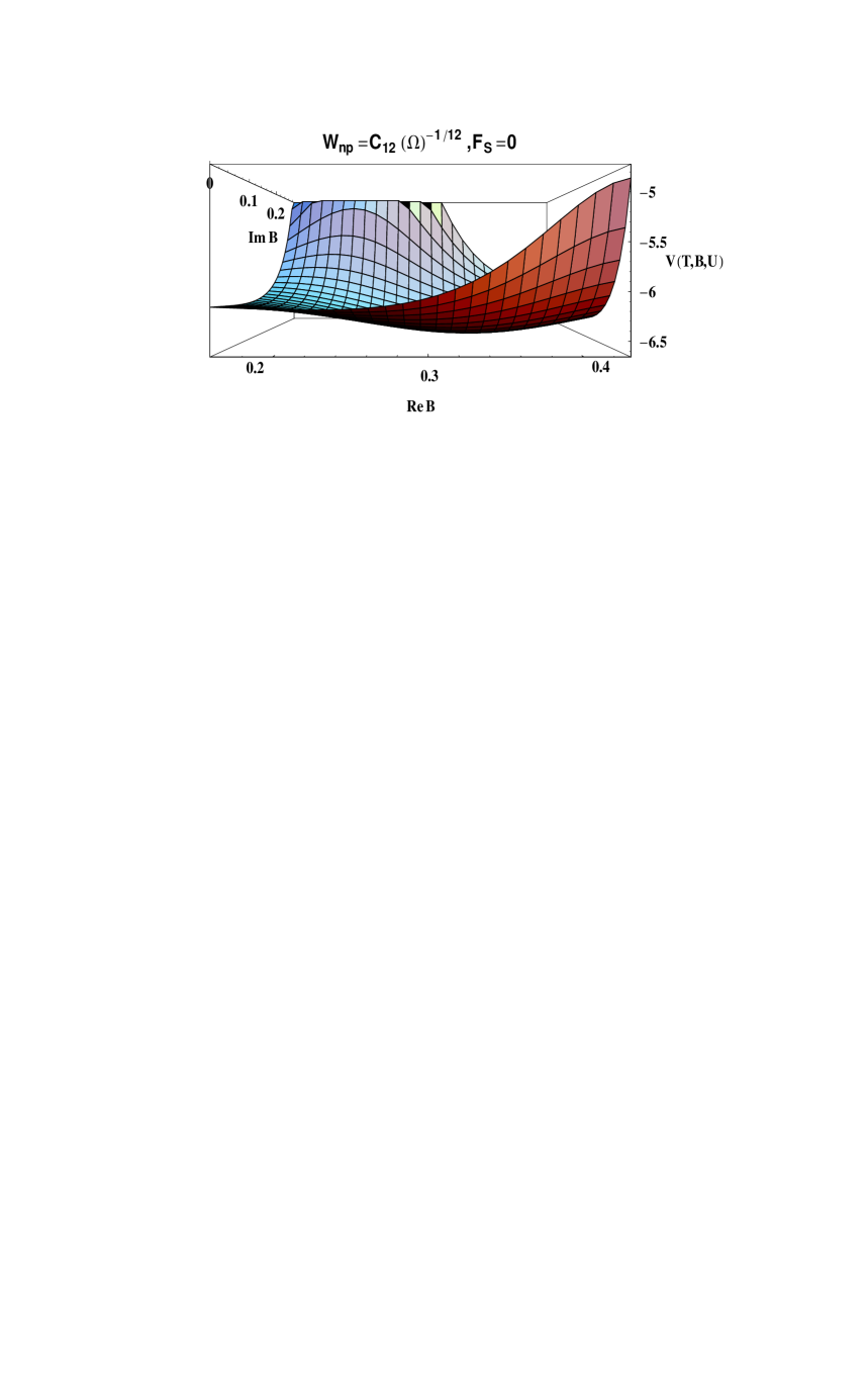
Figure 1: Minimum of $V_{eff}$ in the Wilson line direction

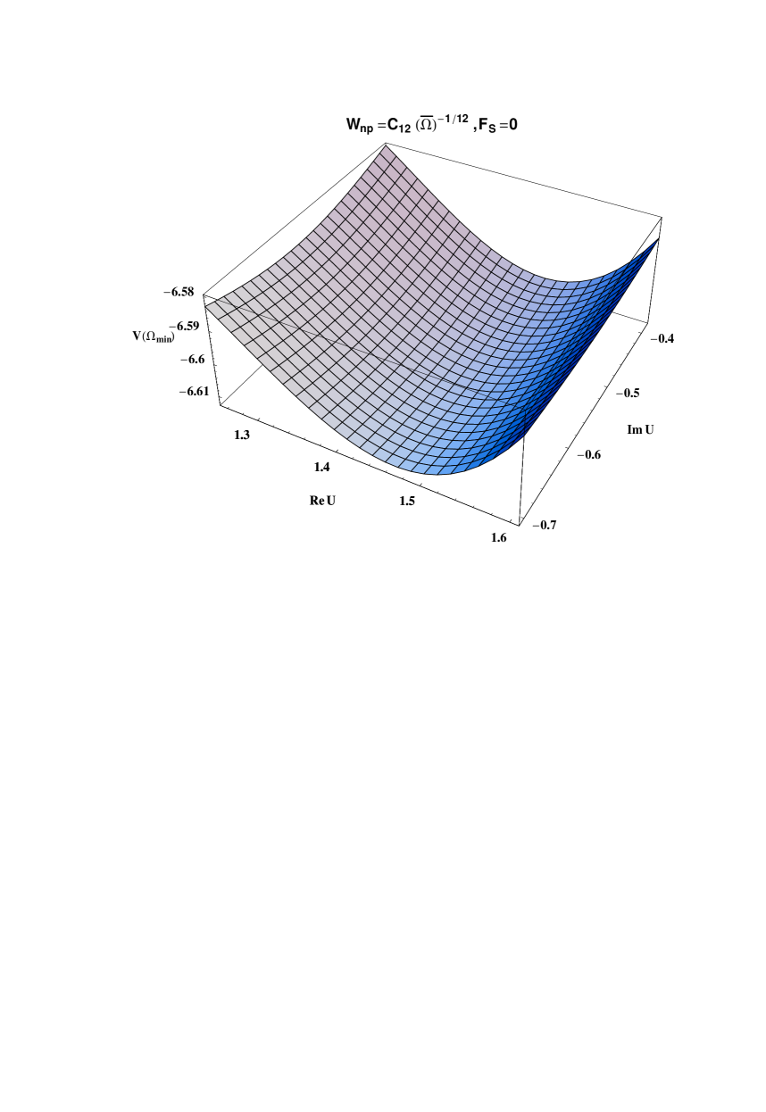
Figure 2: Minimum of $V_{eff}$ in the $U$ direction, see Eq.(13)

One might ask whether the minima obtained correspond to boundary or interior points of a particular “fundamental domain” of $Sp(4,Z)$? According to [12] the matrix of moduli $\Omega$ lies on the boundary of the generalized Siegel fundamental domain $\Im$ if,

$$\Bigl{|}{\rm det}(C\Omega+D)\Bigr{|}=1=\Bigl{|}{\rm det}(-^{t}C\Omega^{{}^{\prime}}+^{t}A)\Bigr{|}$$ (14)

for some choice of

$$\Bigl{(}\begin{array}[]{cc}A&B\\ C&D\end{array}\Bigr{)}\in Sp(4,Z)$$

with $C\not=0$ and $\Omega^{{}^{\prime}}$ the modular transformed matrix of moduli $\Omega$. The matrices $\Omega$ and $\Omega^{{}^{\prime}}$ obtained from (12) and (13) respectively do satisfy these conditions and so are on the boundary. We regard this result as highly non-trivial.

We also find the following (see fig.3-5) minimum

$$T_{min}=1.29861+0.1191744\;i$$

$$B_{min}=1.09051+0.520288\;i$$

$$U_{min}=1.15447+0.194363\;i$$

(15)

together of course with an infinite number of minima connected to it by Siegel modular transformations. For instance we find numerically the following minimum

$$T_{min}=0.56453+1.12787\;i$$

$$B_{min}=0.243256+1.28333\;i$$

$$U_{min}=0.721535+1.20548\;i$$

generated from (15) by the symplectic Siegel modular transformations

$$T \rightarrow \frac{U}{TU-B^{2}}$$

$$B \rightarrow \frac{B}{TU-B^{2}}$$

$$U \rightarrow \frac{T}{TU-B^{2}}$$

We also find the modular transformed minimum under the transformation

$$\Omega\rightarrow A\Omega^{t}A=\Omega^{{}^{\prime}}=\Biggl{(}\begin{array}[]{cc}U&B\\ B&T\end{array}\Biggr{)}$$ (18)

with

$$A=\Biggl{(}\begin{array}[]{cc}0&1\\ 1&0\end{array}\Biggr{)}\in GL(2,Z)$$ (19)

$$T_{min}=U$$

$$B_{min}=B$$

$$U_{min}=T$$

(20)

The above minimum is an interior point since it does not satisfies the Siegel’s equalities (14).

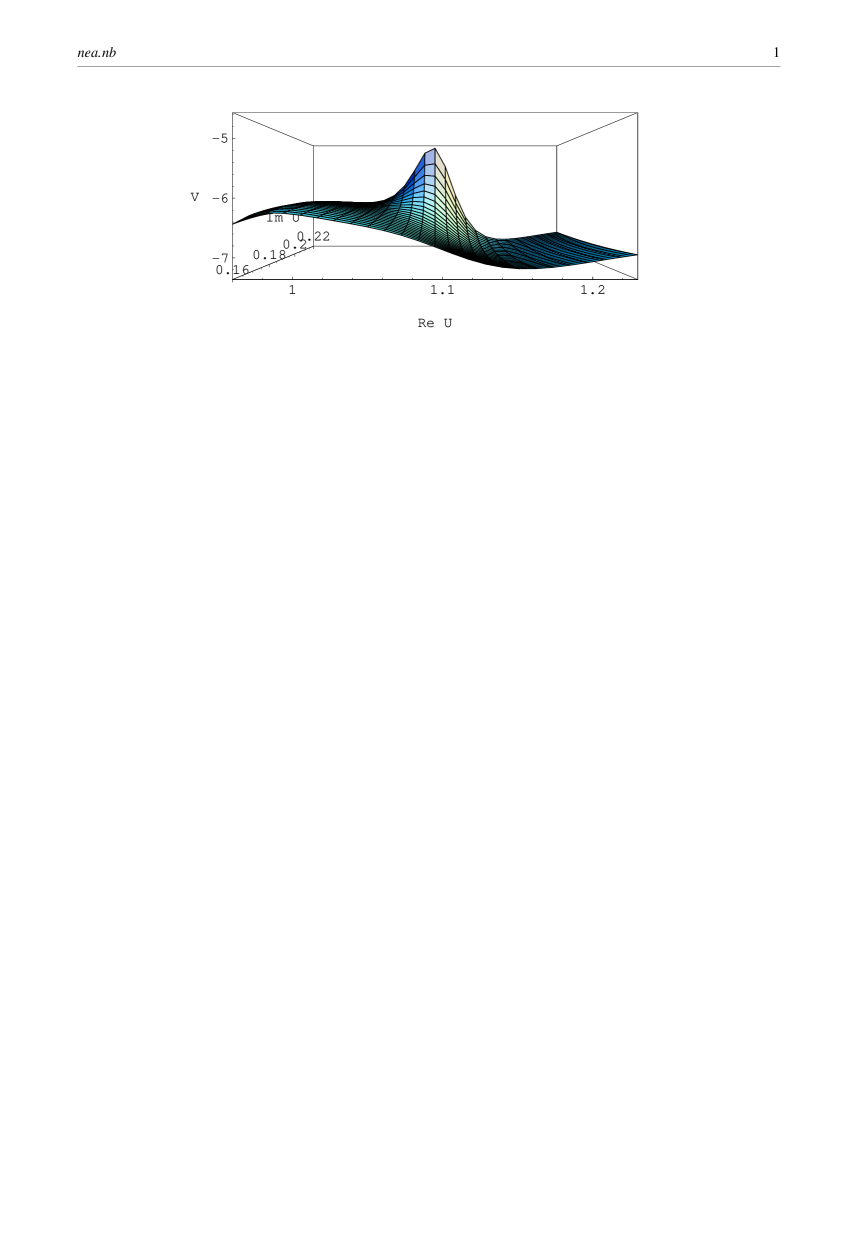
Figure 3: Minimum of $V_{eff}$ in the $U$-direction, see Eq.(15)

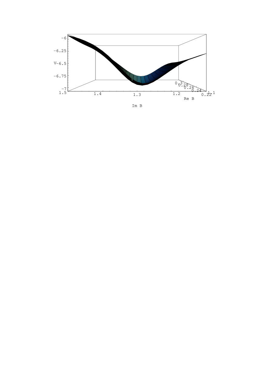
Figure 4: Modular transformed minimum of $V_{eff}$ in the $B$-direction, see Eq.(16)

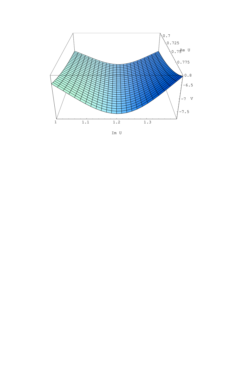
Figure 5: Modular transformed minimum of $V_{eff}$ in the $U$-direction, see Eq.(16)

Interestingly, for large dilaton $F$-terms (i.e $|\frac{dP}{dy}|\gg 1$ and/or $0<\frac{d^{2}P}{dy^{2}}\ll 1$) we obtain familiar algebraic points of the $PSL(2,Z)$ and $\Gamma^{0}(3)$ modular groups. For instance for $\frac{dP}{dy}=1.5$ and $\frac{d^{2}P}{dy^{2}}=0.1$ we (see fig.6-7) obtain

$$T_{min} = \sqrt{3}$$

$$U_{min} = \frac{\sqrt{3}}{2}+\frac{1}{2}\;\;i$$ (21)

with the Wilson line

$$B_{min}=\frac{\sqrt{3}}{2}+\frac{1}{2}\;\;i$$ (22)

As we shall see at this minimum $CP$-violation is zero .

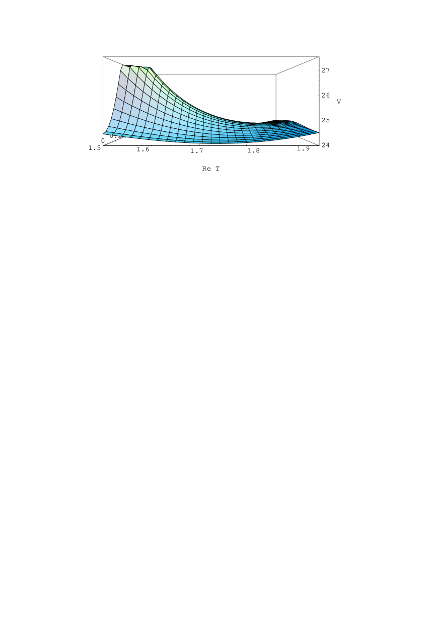
Figure 6: Minimum of $V_{eff}$ in the $T$-direction at the familiar algebraic point of $\Gamma^{0}(3)$

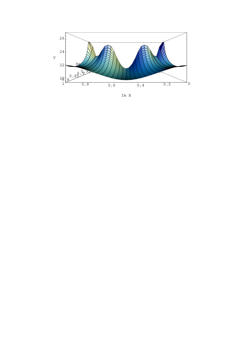
Figure 7: Minimum of $V_{eff}$ in the $B$-direction at the familiar fixed point of $PSL(2,Z)$

We now calculate the $CP$-violation in the $A$ and $B$ terms. Unfortunately in this case (which corresponds to a case of an asymmetric orbifold ) the modular properties of the Yukawa couplings that appear in the trilinear soft $A$-terms in the presence of Wilson line moduli are unknown. In the absence of Wilson line moduli, when the modular groups are $PSL(2,Z)$ and $\Gamma^{0}(3)$ we could cast the twisted sector Yukawa couplings (calculated using conformal field theory techniques) in terms of Jacobi theta functions with definite modular properties [15, 10]. Unfortunately we do not know how to generalize them to Siegel modular forms. However, we study the $CP$-violation arising from the $A$-terms when (i) the Yukawas $h_{\alpha\beta\gamma}$ have no modular dependence, and (ii) the Yukawas $h_{\alpha\beta\gamma}$ are proportional to the appropriate powers of ${\cal C}_{12}(\Omega)$. For $\mu_{W}$ we take the ansatz $\mu_{W}={{\cal C}_{12}(\Omega)}^{1/12}$ for the coupling $\mu_{W}\Phi_{1}\Phi_{2}$ with $\Phi_{1},\Phi_{2}$ both in the untwisted sector. Then in the limit $B\rightarrow 0$, $\mu_{W}\rightarrow\eta^{2}(T)\eta^{2}(U)$ consistent with earlier work by Antoniadis et al [16].

Both $A$ and $B$-terms, in large regions of the parameter space with large auxiliary dilaton $F$-terms, lead to zero $CP$-violating phases. In this case the VEVs of the moduli fields including the Wilson line at the minimum of the effective potential are at familiar algebraic points of the $PSL(2,Z)$ and $\Gamma^{0}(3)$ modular groups. All of the soft terms as well as the $\mu$ term are real. In the moduli dominated limit or in intermediate regions of the auxiliary dilaton-moduli field space soft $B$-terms lead to phases of order $10^{-2}-10^{-1}$. The properties of modular functions offer a pleasing explanation of the approximate $CP$-invariance of the soft supersymmetry-breaking terms. In summary, the picture of the $CP$-structure of the soft supersymmetry breaking terms in the presence of a continuous Wilson line modulus is consistent with the picture that emerged from modular invariant effective actions in which only the metric moduli $T,U$ were present in the effective action [10]. The resulting $CP$-phases are naturally small.

References

• [1] S. Ferrara, D. L$\rm{\ddot{u}}$st, A. Shapere, and S. Theisen, Phys. Lett. B225(1989),363, A. Font, L.E. Ibanez, D. L$\rm{\ddot{u}}$st, and F. Quevedo, Phys. Lett.B 249(1990) 35
• [2] R.Donagi, A.Grassi and E. Witten, Mod.Phys.Lett.A11(1996)2199,hep-th/9607091; G. Curio and D. L$\rm{\ddot{u}}$st, Int. J. Mod. Phys. A12 (1997) 5847,hep-th/9703007
• [3] L.J. Dixon, V. Kaplunovsky and J. Louis, Nucl.Phys. B355(1991) 649
• [4] E. Kiritsis, C. Kounnas, P.M. Petropoulos and J. Rizos, Nucl.Phys.B483(1997)141
• [5] T. Kawai, Phys. Lett. B397(1997)51
• [6] R. Dijkraaf, E. Verlinde and H. Verlinde, Nucl.Phys.B484(1997)543
• [7] G.L. Cardoso, G. Curio and D. L$\rm{\ddot{u}}$st, Nucl. Phys.B491(1997)147, hep-th/9608154
• [8] P. Mayr and S. Stieberger,Phys.Lett.B355(1995)107
• [9] H.P. Nilles and S. Stieberger,Phys.Lett.B367(1996)126; H.P. Nilles and S. Stieberger,Nucl. Phys. B499 (1997) 3
• [10] D. Bailin, G.V. Kraniotis and A. Love, Phys. Lett.B414(1997)269, hep-th/9705244; D. Bailin, G.V. Kraniotis and A. Love, Nucl.Phys.B518(1998)92 hep-th/9707105
• [11] J. Igusa,On the graded ring of theta constants, Am. J. Math.86(1964)219,Am. J. Math.88(1966)221
• [12] C.L. Siegel, Symplectic geometry,Am. J. Math.65(1943)1 and Academic Press New York and London 1964; Analytic functions of several complex variables, Lecture Notes, Institute for Advanced study Princeton N.J.(1948),reprinted 1952.
• [13] K.S Narain, M.H. Sarmadi and C. Vafa, Nucl.Phys.B356(1991) 163
• [14] A. Font, L.E. Ib${\rm a^{{}^{\prime}}\tilde{n}}$ez, D. L$\rm{\ddot{u}}$st and F. Quevedo, Phys. Lett.B 245(1990)401
• [15] E.J. Chun, J. Mas, J. Lauer and H.P. Nilles, Phys.Lett.B233(1989)141; D. Bailin, A. Love and W.A. Sambra, Nucl. Phys. B403 (1993) 265
• [16] I. Antoniadis, E.Gava, K.S. Narain and T.R. Taylor, Nucl. Phys. B432(1994) 187