We compute the entropy of extremal black strings in three dimensions, using Strominger’s approach to relate the Anti-de-Sitter near-horizon geometry and the conformal field theory at the asymptotic infinity of this geometry. The result is identical to the geometric Bekenstein-Hawking entropy. We further discuss an embedding of three-dimensional black strings in $N=1~{}D=10$ supergravity and demonstrate that the extremal strings preserve $1/4$ of supersymmetries.

There has been tremendous interest recently in exploring the proposal that a supergravity theory on an Anti-de-Sitter ($AdS$) space is equivalent to a superconformal theory on the $AdS$ boundary [1, 2, 3]. A strong evidence for this result has been provided by the connection between the isometries of the $AdS$ geometry and the conformal theory on the boundary [4]. This connection is clearly seen in the context of black $p$-branes in supergravity theories, where the near-horizon geometry of a number of extremal supersymmetric $p$-brane systems, either RR or NSNS or both, is $AdS$ [1, 4, 5, 6]. One therefore believes that there must be a natural projection of the bulk theory onto the boundary, and that the boundary theory, like a hologram, retains the information about the bulk degrees of freedom which were projected down [3].

One application of the connection between the bulk supergravity and the boundary conformal field theory has been in the counting of microstates which give rise to the black hole entropy. There are different methods for accomplishing this goal. One approach begins with establishing a $U$-duality map [7] between higher dimensional black holes and the three-dimensional $AdS$ Bañados-Teitelboim-Zanelli (BTZ) black hole [8]. The BTZ black hole is also a solution of string theory [9]. Using $D$-brane method for counting black hole microstates [10, 11], which has been applied with great success in higher dimensions [12, 13], one can show that the $D$-brane count for the BTZ black hole embedded in type II string theory precisely matches the Bekenstein-Hawking formula [7, 14]. However, the $D$-brane counting methods are designed for solutions which can be continued to the weak coupling regime. It is of interest to see how one can count microstates in the strong coupling, when the black hole causal structure is manifest. Using the U-duality-generated trans-dimensional chart of related solutions [15], Sfetsos and Skenderis have reproduced the Bekenstein-Hawking formula for a number of solutions [16], which can be arbitrarily far from extremality. They have obtained the entropy using Carlip’s approach [17] to count the microstates of the BTZ black hole formulated as a solution of topological $2+1$ gravity. In this case, one counts the entropy by associating degrees of freedom to the horizon, which explains why the entropy of the hole is measured by the horizon area, and not by the volume of the space excised from the spacetime to accommodate the hole. However this is based on the description of the BTZ hole by a purely topological Chern-Simons formulation, which is not a fundamental description of a sector of string theory. Another, more direct, method of counting the entropy has been proposed recently by Strominger [18]. Similar approach has also been advocated by Birmingham, Sachs and Sen [19]. This method is based on the fact that if a solution of a dynamical theory of gravity has a region which is approximated by $AdS_{3}$ geometry, one can construct a conformal field theory (CFT) on the boundary of $AdS_{3}$. The boundary theory can be determined by studying the large distance limit of diffeomorphisms in the $AdS$ bulk [21]. The $AdS$ boundary need not be the physical infinity of the spacetime, but the limit of validity of the $AdS$ approximation to the bulk solution. On the $AdS_{3}$ boundary, the “large” diffeomorphisms cease to be integrable, and acquire local dynamics [20, 21, 17, 22]. Their dynamics is given by a CFT, and one can determine the degeneracy of a black hole macrostate by counting different microstates of the CFT which correspond to the same black hole solution. This should match the Bekenstein-Hawking formula. Similar investigations have been successfully carried out for the BTZ black hole [18, 19], the whole of de-Sitter space [24], and some 5D (near)extremal black strings with the near-horizon geometry approximated by a (near)extremal BTZ hole [25]. For other uses, see also [26].

In this article, we discuss a simple realization of the boundary conformal theory for extremal three-dimensional black strings, constructed by Horne and Horowitz [28] prior to the discovery of the BTZ black hole. This solution in fact corresponds to the throat limit of a fundamental string inside an NS $5$-brane, as we will discuss later [29]. Near the horizon, the scalar dilaton is fixed, approaching a constant value very quickly. Hence the near-horizon geometry of this solution is $AdS_{3}$. Therefore, we can straightforwardly apply Strominger’s procedure [18], up to the distances of order of $\sqrt{Ml}$ away from the horizon, where $M$ corresponds to the mass per unit length of the string. The near-horizon limit of the dilaton and the NSNS $3$-form specify the effective Newton’s constant and the cosmological constant, which in turn define the CFT central charge and normalization. This suffices to specify the Virasoro algebra of the boundary CFT. In order to find the degeneracy of the string solution from the boundary CFT, we use the fact that this Virasoro algebra is faithfully reproduced by the boundary CFT of the topological Chern-Simons $SO(2,2)$ gravity. The boundary degrees of freedom are in one-to-one correspondence with the large gauge transformations in the bulk, and we can compute the number of states using the microcanonical ensemble approach of [27]. In the course of our calculation, we encounter an interesting subtlety: we must regularize the expressions for the boundary CFT. The proper regularization of the theory consists of considering a near-extremal solution, and compactifying the length along the string with a period inversely proportional to the Hawking temperature. This reproduces the correct expression for the statistical entropy, which matches exactly the Bekenstein-Hawking formula for the extremal black string. Finally, we show how black strings arise as consistent supersymmetric solutions preserving $1/4$ of supersymmetries of $N=1~{}D=10$ supergravity.

We first review here the black string family of [28], with the attention on the entropy. To construct a $3D$ black string solution, we look for the static extrema of the low-energy action

$$I_{3}=\frac{1}{16\pi G}\int d^{3}x\sqrt{g}e^{-\phi}\Bigl{(}R+(\nabla\phi)^{2}-\frac{1}{12}H^{2}_{\mu\nu\lambda}+\frac{4}{l^{2}}\Bigr{)}$$ (1)

where in addition to the metric $g_{\mu\nu}$ we have the dilaton $\phi$ and the NSNS $2$-form field strength $H_{\mu\nu\lambda}=\partial_{\mu}B_{\nu\lambda}+cyclic~{}permutation$. The term $\Lambda=-2/l^{2}$ plays role of the effective (negative) stringy cosmological constant, and can arise if the central charge of the three-dimensional theory is not equal to the dimension of the spacetime. In the Wess-Zumino-Witten construction of [28], it is given by the level of the Kač-Moody algebra $l^{2}=k/2$. The cosmological term can also arise from dimensional reductions on internal manifolds with nonabelian symmetry. We will give an example later.

The static black string family which emerges from (1) is given by

$$ds^{2} = -\bigl{(}1-\frac{M}{r}\bigr{)}dt^{2}+\bigl{(}1-\frac{Q^{2}}{Mr}\bigr{)}dx^{2}+\frac{l^{2}dr^{2}}{4(r-M)(r-Q^{2}/M)}$$ (2)

$$H=\frac{Q}{r^{2}}~{}dt\wedge dx\wedge dr~{}~{}~{}~{}~{}~{}~{}~{}~{}~{}~{}~{}~{}~{}~{}~{}~{}e^{-\phi}=~{}\frac{r}{l}$$

The parameters $M$ and $Q$ correspond to the ADM mass per unit length of the string, and the axion charge per unit length, respectively. They are related to the mass $m$ and spin $j$ of the dual BTZ black hole, in the notation of [18], according to $M=4G(ml+\sqrt{m^{2}l^{2}-j^{2}})$ and $Q=4Gj$, and have the dimension of length. We have normalized the solution such that the case $M=Q=0$ corresponds to the linear dilaton solution of [30], which is the black string vacuum. This solution is asymptotically flat (in the string frame) as $r\rightarrow\infty$, has an event horizon at $r_{+}=M$, a Cauchy horizon at $r_{-}=Q^{2}/M$, and a curvature singularity at $r\rightarrow 0$. The singularity is reached by all future-oriented null geodesics, and hence the manifold is geodesically incomplete. There is a subtlety in defining the complete Penrose diagram of this solution. The diagram should be three-dimensional to accommodate the interplay between the coordinates $t$ and $x$, and the details can be found in [28].

A black string emits Hawking radiation to ${\cal J}^{+}$, and looses energy while its charge is conserved because of the Gauss law for $H$. The dynamics of emission is that of a black body with the Hawking temperature $T_{H}$, which can be determined after a simple Wick rotation $t\rightarrow i\tau$. Near the event horizon, $r\rightarrow r_{+}=M$, we recover the Euclidean metric in cylindrical polar coordinates, which is smooth near the origin if we identify the Euclidean time with the period $2\pi lM/(M^{2}-Q^{2})$. Hence the Hawking temperature of the black string is

$$T_{H}=\frac{\sqrt{M^{2}-Q^{2}}}{2~{}\pi lM}$$ (3)

Clearly, the temperature vanishes when $M$ reduces to $Q$, and the resulting solution ceases to emit Hawking radiation. This corresponds to the extremal limit of the black string. The horizon is still at $r_{+}=M$. It is tempting to think that the analytic continuation across the horizon is accomplished by going to $r<M$. However, this is not true [28]. The coordinate $r$ cannot be continued across the horizon, which is a fixed point for $r$. But this is only an artifact of a bad coordinate system. The correct continuation is performed with choosing the new radial coordinate $\rho$ according to $r=M+\rho^{2}/l$, and letting $\rho$ pass through zero, which is the location of the horizon in the new coordinate system [28]. In terms of the new radial coordinate, the solution is

$$~{}~{}~{}~{}~{}ds^{2}=\frac{\rho^{2}}{Ml+\rho^{2}}\bigl{(}-dt^{2}+dx^{2}\bigr{)}+\frac{l^{2}d\rho^{2}}{\rho^{2}}$$

$$H = \frac{2Ml\rho}{(Ml+\rho^{2})^{2}}~{}dt\wedge dx\wedge d\rho~{}~{}~{}~{}~{}~{}~{}~{}~{}~{}~{}~{}~{}e^{-\phi}=\frac{Ml+\rho^{2}}{l^{2}}$$ (4)

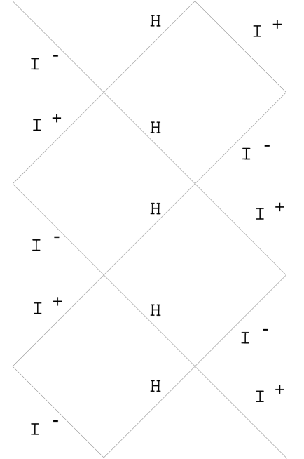
Figure 1: Maximal extension of the extremal Horne-Horowitz black string. H denotes the event horizon, and I⁺ and I^- future and past null infinity, respectively.

The solution is invariant under $\rho\leftrightarrow-\rho$, which implies that the universe behind the event horizon is a mirror image of the original one. Hence the maximal extension of this solution is an infinite array of asymptotically Minkowski diamonds aligned along a zig-zag event horizon, as mentioned before. This is illustrated in Figure 1.

The Bekenstein-Hawking entropy is in general given as one quarter of the area of event horizon, $S_{BH}={\cal A}/(4G_{N})$, in Planck units. This formula is expected to work well for sufficiently large configurations, where we can trust the classical theory close to the event horizon. The normalization of the entropy is given in the units set by the normalization of the Einstein term in the action, $\sim\int d^{D}x\sqrt{g}R/(16\pi G_{N})$. For the black string in the string frame, the Newton’s constant is $G_{N}=G\exp(\phi(r_{+}))$, as can be verified from (1). The “area” in this case is just the proper length of the string. It is given by ${\cal A}=\int\sqrt{g_{xx}(r_{+})}dx=\sqrt{M^{2}-Q^{2}}L/M$, where $L=\int dx$ is the comoving length of the string. Hence substituting these formulas, we find

$$S_{BH}=\frac{{\cal A}}{4G}e^{-\phi(r_{+})}=\frac{L}{4Gl}\sqrt{M^{2}-Q^{2}}$$ (5)

For fixed $M$ and $Q$, this expression diverges as $L\rightarrow\infty$, which corresponds to an infinite string. However, the entropy per unit length is given by $S_{BH}/L=\sqrt{M^{2}-Q^{2}}/(4Gl)=\pi MT_{H}/(2G)$, and it is finite (and vanishing when $T_{H}=0$). This suggests that in order to consider the entropy of the string we can break up the whole string into an infinite array of identical “elementary strings”, each of them being a $T$-dual image of a BTZ black hole. In effect, we formally compactify the coordinate along the string on a circle of circumference $L$, and then view the infinite string as the covering space of an elementary segment [32]. The length of the elementary segment can be determined by comparing it to the $T$-dual BTZ hole. Following [32], after straightforward algebra we find it to be

$$L=2\pi l\sqrt{\frac{Ml}{M^{2}-Q^{2}}}$$ (6)

Substituting this expression in the formula for the Bekenstein-Hawking entropy, we find that the entropy of each elementary string segment is

$$S_{BH}=\frac{\pi}{2G}\sqrt{Ml}$$ (7)

Using the picture where the string is broken into elementary segments ensures that the formula (7) for the Bekenstein-Hawking entropy is valid in the extremal limit. This may sound a little odd, since as we have seen above, the entropy per unit length of the string is directly proportional to the Hawking temperature of the string, and hence zero in the extremal limit. However, the length $L$ of the elementary segments of a string diverges as $M\rightarrow Q$. In the extremal limit, the whole infinite string should be viewed as a single elementary segment itself. This is deduced from the fact that this extremal string is dual to the extremal spinning BTZ black hole [9, 32]. A spinning black hole in turn can be obtained by boosting a static hole along the circle and identifying the boosted coordinate. The extremal limit corresponds to the infinite Lorentz boost, and the fact that the dual extremal string must be infinite arises from the need to compensate for the (inverse) Lorentz-contraction of the azimuthal angle of the BTZ hole. The nonvanishing total entropy $S_{BH}=\frac{\pi}{2G}\sqrt{Ml}$ can be viewed as the zero point entropy of the extremal black string.

Now we can proceed to compute the statistical entropy of the black string system, using the proposal of [18]. This should be applicable, since the near-horizon geometry of the extremal black string is approximately $AdS$. We first sketch the calculation, and point out a subtlety which arises in its course. Using the solution (4), we see that as $\rho\rightarrow 0$, the metric approaches

$$ds^{2}=\frac{\rho^{2}}{Ml}\bigl{(}-dt^{2}+dx^{2}\bigr{)}+\frac{l^{2}d\rho^{2}}{\rho^{2}}$$ (8)

which is clearly $AdS$. In this limit, $H^{2}=-\frac{24}{l^{2}}\frac{M^{2}l^{2}}{(Ml+\rho^{2})^{2}}\rightarrow-\frac{24}{l^{2}}$ and also $(\nabla\phi)^{2}=\frac{4\rho^{4}}{l^{2}(Ml+\rho^{2})^{2}}\rightarrow 0$. The effective action is approximated by

$$S_{eff}=\frac{M}{16\pi Gl}\int d^{3}x\sqrt{g}\Bigl{(}R+\frac{2}{l^{2}}\Bigr{)}$$ (9)

The effective cosmological constant is half of the value of the stringy cosmological constant $2/l^{2}$ due to the contribution of the $3$-form field strength: $1/l^{2}_{eff}=2/l^{2}+H^{2}/24=2/l^{2}-1/l^{2}=1/l^{2}$. The sign in the first equation is plus, because the solution for $H$ must be inserted into the action with care, using the Lagrange multiplier method [33]. Hence, near the horizon, the only effect of the dilaton and the $3$-form is to renormalize the Newton’s constant and the cosmological constant of the effective theory, which become

$$G_{N}=\frac{Gl}{M}~{}~{}~{}~{}~{}~{}~{}~{}~{}~{}~{}\Lambda_{eff}=\frac{1}{l^{2}}$$ (10)

The remainder of the counting procedure is to find the boundary CFT and count the density of states. According to [18, 19], the boundary CFT is given by the projections of the “large” diffeomorphisms of the bulk theory at asymptotic infinity. A black string macrostate is specified by the $SL(2,R)$ sector of the boundary Virasoro algebra. This information is encoded in the long-distance behavior of the dreibein and the spin connexion. To obtain it, we resort to the Chern-Simons gauge theory formulation of three-dimensional gravity, with the same Newton’s constant and cosmological constant. This theory produces a faithful representation of the boundary Virasoro algebra, which is homomorphic with the string boundary CFT, since both are given by the “large” diffeomorphisms. We will use the microcanonical ensemble approach of [27] to find the degeneracy of the boundary theory.

If we straightforwardly proceed in this direction, we encounter an undetermined expression for the entropy of the type $0\cdot\infty$. This ambiguity arises because in the extremal limit the Hawking temperature vanishes, while the circle spanned by the $x$ coordinate decompactifies. We have encountered the same problem earlier, while determining the Bekenstein-Hawking entropy of the extremal solution. Indeed, in the statistical approach, as [27] show, the expressions for the number of chiral states on the boundary involve integrations over $x$, which diverges as $M\rightarrow Q$. This is multiplied by the number density of the states on the boundary, which is essentially given by the mass and the spin of the metric in the $AdS$ limit. By comparing the metric (8) to the BTZ solution in this limit, we see that in the $AdS$ limit the solution (4) is approximated by the $M=J=0$ BTZ hole. Naively, this suggests that the number density of the states on the boundary vanishes. Ergo, we end up with $S\sim 0\cdot\infty$.

Hence we must first regularize the solution. We do it by considering near-extremal solutions, with $M^{2}=Q^{2}+\epsilon^{2}$, in the near-horizon limit. Thus we have $Q^{2}=M^{2}-\epsilon^{2}$, and we keep $\rho^{2}=r-M$. The metric becomes

$$ds^{2}=-\frac{\rho^{2}}{Ml+\rho^{2}}dt^{2}+\frac{\rho^{2}+l\epsilon^{2}/M}{Ml+\rho^{2}}dx^{2}+\frac{l^{2}d\rho^{2}}{\rho^{2}+l\epsilon^{2}/M}$$ (11)

The $3$-form and the dilaton still give $H^{2}\rightarrow-\frac{24}{l^{2}}$, $(\nabla\phi)^{2}\rightarrow 0$ in the limit $\rho,\epsilon\rightarrow 0$, implying that our near-horizon approximation is valid up to distances $\rho\sim\sqrt{Ml}$. To define the boundary CFT, we recall that the effective action is still given by (9), with the same values of the Newton’s and cosmological constants as before. The boundary CFT algebra corresponds to the “large” diffeomorphisms of this theory. We recall that the only effect of the matter is to renormalize the “bare” cosmological constant and Newton’s constant. Since the bulk is $AdS_{3}$, its symmetry group is $SO(2,2)\sim SL(2,R)\times SL(2,R)$. Hence the boundary algebra splits into a direct product of two disjoint copies of the Virasoro algebra [21]. When the boundary is compactified to a cylinder, which is the case of our elementary segments, we can write the Virasoro algebras in terms of the Fourier modes of the diffeomorphism generators on the boundary:

$$[L_{m},L_{n}]=i(m-n)L_{m+n}+i\frac{c}{12}(m^{3}-m)\delta_{m+n,0}$$ (12)

each with the central charge

$$c=\frac{3l_{eff}}{2G_{N}}$$ (13)

For the values of $G_{N}$ and $l_{eff}$ in (10), the central charge is $c=\frac{3M}{2G}$. In order to determine the degeneracy of the black string, which corresponds to its entropy, we need to evaluate the eigenvalues of the operators $L_{0}$ and $\bar{L}_{0}$ in the background (11). For the BTZ hole, this leads to simple expressions where $L_{0}=Ml+J$ and $\bar{L}_{0}=Ml-J$. But as we have pointed out above, this would lead to the incorrect expressions $L_{0}=\bar{L}_{0}=0$ for the case of the extremal string. We can correctly determine $L_{0}$ and $\bar{L}_{0}$ using the microcanonical ensemble method of [27] instead. As we have noted above, according to [18], we should consider the large distance limit of diffeomorphisms of the bulk gravity near the horizon (9). After choosing the proper gauge, these give rise to local degrees of freedom on the boundary that determine the boundary CFT. Given the near-horizon specification of the geometry in terms of the mass and charges, we can count different microstates that produce the same mass and charges to find the entropy. For this purpose, we do not need the exact construction of the boundary CFT, but merely a faithful representation of its Virasoro algebras. To this end, we can consider the topological Chern-Simons gauge theory on $SO(2,2)$ [31]. This theory is the effective description of only the diffeomorphism sector, since it contains no local degrees of freedom. Since $SO(2,2)\sim SL(2,R)\times\bar{SL}(2,R)$, one can rewrite the action (9) as a linear combination of two copies of the Chern-Simons gauge theory on $SL(2,R)$. The tangent space Hodge dual of the spin connection is $\omega^{a}=\frac{1}{2}\epsilon^{abc}\omega_{bc}$, and the gauge fields are $A^{a}_{\pm}=(\omega^{a}\pm\frac{1}{l}e^{a})J_{a}$, where $J^{a}$ are the $SL(2,R)$ generators, given in terms of the Pauli spin matrices as $J_{0}=(i/2)\sigma_{2}$, $J_{1}=(1/2)\sigma_{3}$ and $J_{2}=(1/2)\sigma_{1}$. The inner product on the algebra is $<J_{a},J_{b}>=Tr(J_{a}J_{b})=(1/2)\eta_{ab}$, where $\eta_{ab}$ is the tangent space metric. The dreibein $e^{a}$ and the dual spin connection $\omega^{a}$ are treated as independent variables, and the structure equation $de^{a}+\epsilon^{abc}e_{b}\wedge\omega_{c}=0$ is obtained as the $\omega_{a}$ equation of motion. The Chern-Simons action which yields the same equations of motion as (9), after the $3D$ metric is defined by $g_{\mu\nu}=\eta_{ab}e^{a}{}_{\mu}e^{b}{}_{\nu}$, is

$$I_{eff}=I_{+}-I_{-}$$ (14)

where the Chern-Simons actions for the left and right chiral gauge fields are

$$I_{\pm}=\frac{M}{16\pi G}\int<A_{\pm}\wedge dA_{\pm}+\frac{2}{3}A_{\pm}\wedge A_{\pm}\wedge A_{\pm}>$$ (15)

The bulk equations of motion for the Chern-Simons gauge theory are $F^{a}_{\pm}=0$, i.e. the gauge fields in the bulk are pure gauge, $A^{a}_{\pm}=2\eta^{ab}Tr(J_{b}g_{\pm}^{-1}dg_{\pm})$. We can calculate the gauge fields as follows. Because we are considering the near-extremal string, the boundary is a simple tensor product $R\times S^{1}$, where the circle is parameterized by $x$. It is instructive to normalize the coordinate along the circle to run from $0$ to $2\pi$. This is assured by defining the angle $\theta=2\pi x/L$, where $L$ has been given in (6). Changing the variable $\rho$ to $\rho=\sqrt{l/M}\epsilon\sinh(\vartheta)$, with some simple algebra, we find the dreibein and the dual spin connexion at an arbitrary value of $\vartheta$ and in the limit $\epsilon=0$ (where we have also rescaled the time $t=\sqrt{M/l}(L/2\pi)\tau$ to the Wick-rotated Euclidean time):

$$e^{0}=l\sinh(\vartheta)d\tau~{}~{}~{}~{}~{}~{}~{}~{}~{}~{}~{}~{}~{}~{}~{}e^{1}=ld\vartheta~{}~{}~{}~{}~{}~{}~{}~{}e^{2}=\frac{l^{3/2}}{\sqrt{M}}\cosh(\vartheta)d\theta$$

$$\omega^{0}=\sqrt{\frac{l}{M}}\sinh(\vartheta)d\theta~{}~{}~{}~{}~{}~{}~{}~{}~{}\omega^{1}=0~{}~{}~{}~{}~{}~{}~{}~{}~{}~{}~{}\omega^{2}=\cosh(\vartheta)d\tau$$ (16)

Using now $A^{a}_{\pm}=\omega^{a}\pm\frac{1}{l}e^{a}$, we find the gauge fields

$$A^{0}_{\pm}=\sinh(\vartheta)\frac{\sqrt{l}d\theta\pm\sqrt{M}d\tau}{\sqrt{M}}~{}~{}~{}~{}~{}~{}A^{1}_{\pm}=\pm d\vartheta~{}~{}~{}~{}~{}~{}A^{2}_{\pm}=\cosh(\vartheta)\frac{\sqrt{M}d\tau\pm\sqrt{l}d\theta}{\sqrt{M}}$$ (17)

The Lie-algebra valued $1$-form gauge field is

$$A_{\pm}~{}=~{}\frac{1}{2}\pmatrix{\pm d\vartheta&e^{\mp\vartheta}\frac{\sqrt{M}d\tau\pm\sqrt{l}d\theta}{\sqrt{M}}\cr e^{\pm\vartheta}\frac{\sqrt{M}d\tau\pm\sqrt{l}d\theta}{\sqrt{M}}&\mp d\vartheta\cr}$$ (18)

Now we must choose the gauge as $\vartheta\rightarrow\infty$. This is best accomplished by choosing the radial components $A_{\pm\vartheta}=g^{-1}_{\pm}\partial_{\vartheta}g_{\pm}=\frac{1}{2}~{}diag(\pm 1,\mp 1)$, from which we find the matrix

$$g_{\pm}~{}=~{}\pmatrix{e^{\pm\vartheta/2}&0\cr 0&e^{\mp\vartheta/2}\cr}$$ (19)

We can use this matrix to transform to the gauge $A_{\pm~{}a}(t,\theta)=g_{\pm}A_{\pm~{}a}(\vartheta,\tau,\theta)g^{-1}_{\pm}$. In this way, we project out the radial dependence and obtain the CFT representation at any $\vartheta$. In particular, we find $A_{\pm\theta}(\theta)=\pm\sqrt{\frac{l}{M}}J_{2}$. Hence, $A^{2}_{\pm\theta}=\pm\sqrt{l/M}$. These gauge fields can be used to construct the boundary Virasoro charges. Using our notation and the definitions of [27] we find

$$L_{0}=\frac{M}{32\pi G}\int\eta_{ab}A^{a}_{+\theta}~{}A^{b}_{+\theta}d\theta=\frac{l}{16G}$$ (20)

and, similarly, also $\bar{L}_{0}=l/(16G)$. Here we have dropped an irrelevant constant term, since we normalize the entropy to be zero in the linear dilaton vacuum. Since the Cardy formula for degeneracy of states of a conformal field theory with central charge $c$ and excitations $n_{L}=L_{0}$ and $n_{R}=\bar{L}_{0}$ [23] is valid for $1<<c<<n_{L}+n_{R}$, we must have $G<<M<<l/8$. But this is precisely the classical limit of the black string, where we trust the solution. Hence we have

$$S=2\pi\sqrt{\frac{c}{6}}\bigl{(}\sqrt{n_{L}}+\sqrt{n_{R}}\bigr{)}$$ (21)

We find, substituting our expressions,

$$S=\frac{\pi}{2G}\sqrt{Ml}$$ (22)

i.e. precisely the Bekenstein-Hawking formula. Hence we see that the counting of the conformal degrees of freedom exactly reproduces the geometric entropy of the extremal black string.

Originally, black string solutions in three dimensions have been considered as solutions of the bosonic string theory, where they have been implemented as exact gauged $SL(2,R)\times R/R$ Wess-Zumino-Witten models. However such black strings arise in any superstring theory. They correspond to the throat limit of a fundamental string inside an NS $5$-brane [29]. They can be represented as compactifications on a three-sphere of $N=1~{}D=10$ supergravity theory, which is a consistent low energy truncation of any superstring theory. If we consider only the NSNS fields, in any $10D$ superstring theory we have

$$I=\int d^{10}x\sqrt{\hat{g}}e^{-\hat{\phi}}\Bigl{(}\hat{R}+(\hat{\nabla}\hat{\phi})^{2}-{1\over 12}\hat{H}^{2}\Bigr{)}$$ (23)

where the caret denotes $10D$ quantities. Supersymmetry of toroidal compactifications of this theory to three dimensions has been studied in [34, 35]. We can now consider compactifying this action to three dimensions in a different way, assuming that the manifold splits as $M_{10}=M_{3}\times S^{3}\times T^{4}$, and that the internal $4$-torus is trivial, i.e. that it decouples. Setting all its internal moduli fields to $1$, for simplicity, we see that the $10D$ and $6D$ fields are identical. Now, we can reduce further on an $S^{3}$. We take

$$d\hat{s}^{2}=g_{\mu\nu}dx^{\mu}dx^{\nu}+r^{2}(x)d\Omega_{3}$$ (24)

The scalar field $r(x)$ is the radius of the internal sphere. We will require that the NSNS $3$-form field is nonzero on the $S^{3}$, given by the monopole configuration

$$H_{abc}=\sqrt{2}Q\sqrt{\Omega_{3}}\epsilon_{abc}$$ (25)

such that $H^{2}/12=Q^{2}/r^{6}$. When we reduce the dilaton to $2+1$ dimensions, we find $\exp(-\phi)=r^{3}\exp(-\hat{\phi})$. Further, the Ricci scalar upon reduction produces an additional “scalar potential” term $\sim 1/r^{2}$. The reduced $3D$ action is

$$I_{3}=\int d^{3}x\sqrt{g}e^{-\phi}\Bigl{(}R+(\nabla\phi)^{2}-\frac{1}{12}H^{2}_{\mu\nu\lambda}-3\frac{(\nabla r)^{2}}{r^{2}}+\frac{6}{r^{2}}-\frac{Q^{2}}{r^{6}}\Bigr{)}$$ (26)

This expression arises since the $6D$ Ricci curvature splits into $\hat{R}=R+6/r^{2}-6\nabla^{2}r/r-6(\nabla r/r)^{2}$, where covariant derivatives are taken with respect to the $3D$ spacetime metric. The $\sim\nabla^{2}r$ term is integrated by parts, and the action is, up to a boundary term, given by (26).

We choose the parameters $Q,r_{0}$ such that there exist solutions with $r=r_{0}=const$. In this way, we recover the action (1), where supersymmetry is inherited from $N=1~{}D=10$ supergravity. The condition relating the radius of the $S^{3}$ and the monopole charge is $r^{2}_{0}=|Q|/\sqrt{2}$. This theory is equal to our original action (1) in three dimensions if we choose $r_{0}=\sqrt{2}l$. This gives us the quantization condition for the radius $r_{0}$, if we consider the black string as a WZW model. We can write the extremal string solution as an exact $10D$ configuration

$$~{}~{}d\hat{s}^{2}=\frac{\rho^{2}}{Ml+\rho^{2}}(-dt^{2}+dx^{2})+\frac{l^{2}d\rho^{2}}{\rho^{2}}+2l^{2}d\Omega_{3}+d\vec{y}^{2}_{4}$$

$$\hat{H} = 2\frac{Ml\rho}{(Ml+\rho^{2})^{2}}dt\wedge dx\wedge d\rho+4l^{2}\sqrt{\Omega_{3}}~{}\vec{V}_{3}~{}~{}~{}~{}~{}~{}~{}~{}e^{-\hat{\phi}}=\frac{Ml+\rho^{2}}{l^{2}}$$ (27)

which is clearly very similar to the self-dual dyonic string in $6D$ [36] lifted to $10D$. An important difference is that the “harmonic” form multiplying the transversal section of the metric has been shifted by a $-1$ (using the standard terminology where $h=1+q/\vec{r}^{D-3}$), similar to the $U$-duals of other string solutions [7, 15]. If we Hodge-dualize the magnetic part of the $3$-form to a $7$-form, we can recognize the $5$-brane contribution, to which the solution reduces exactly when $M=0$. Hence $M$ measures the charge of the fundamental string, as is clear from the electric part of the $3$-form.

We will now show that our solution preserves $1/4$ of supersymmetries of $N=1~{}D=10$ supergravity, similarly to the selfdual dyonic string [36]. We can see this as follows. The string-frame supersymmetry transformation rules for the $N=1~{}D=10$ fermions are [37]

$$\delta\lambda=-\frac{1}{4\sqrt{2}}\Gamma^{M}\partial_{M}\hat{\phi}\zeta+\frac{1}{24\sqrt{2}}\Gamma^{MNK}\hat{H}_{MNK}\zeta$$

$$~{}~{}~{}~{}~{}~{}~{}\delta\psi_{M}=\partial_{M}\zeta+\frac{1}{4}\Omega_{-~{}M}{}^{NK}\Gamma_{NK}\zeta$$ (28)

The indices $\{M,N,K\}$ run over the $10D$ tangent space, and the quantity $\Omega_{-~{}M}{}^{NK}=\hat{\omega}_{M}{}^{NK}-\frac{1}{2}\hat{H}_{M}{}^{NK}$ is the generalized spin connexion. The matrices $\Gamma^{M}$ comprise the $10D$ Clifford algebra, and $\Gamma^{M_{1}M_{2}...M_{k}}=\Gamma^{[M_{1}}\Gamma^{M_{2}}...\Gamma^{M_{k}]}$ is their antisymmetrized product. If there exists a spinor $\zeta$ such that $\delta\lambda=\delta\psi_{M}=0$, the solution possesses unbroken supersymmetries. Let us determine the conditions which $\zeta$ must satisfy. Since $\Gamma^{M}\partial_{M}\hat{\phi}=-\frac{\sqrt{2}}{l}\frac{\rho^{2}}{Ml+\rho^{2}}\Gamma^{1}$ and $\frac{1}{6}\Gamma^{MNK}\hat{H}_{MNK}=\frac{\sqrt{2}}{l}\frac{Ml}{Ml+\rho^{2}}\Gamma^{1}\Gamma^{0}\Gamma^{2}+\frac{\sqrt{2}}{l}\Gamma^{3}\Gamma^{4}\Gamma^{5}$, we see that requiring $\delta\lambda=0$ gives two conditions on $\zeta$:

$$(1-\Gamma^{0}\Gamma^{2})\zeta=0~{}~{}~{}~{}~{}~{}~{}~{}(1+\Gamma^{1}\Gamma^{3}\Gamma^{4}\Gamma^{5})\zeta=0$$ (29)

The chirality condition of $N=1~{}D=10$ supergravity is $\Gamma^{11}\zeta=\zeta$. This means that our two conditions are independent. Hence our solution selects $1/4$ of the available spinors. We now turn our attention to $\delta\psi_{M}$. Since the solution (4) is a simple tensor product $M_{3}\times S^{3}$, the spinors split into a $3D$ part and a spherical part. The sphere is maximally supersymmetric, and we do not get any new constraints on $\zeta$ from $\delta\psi_{M}$ in $S^{3}$. Then, assuming that $\zeta$ is independent of the coordinates $t,x$, it is straightforward to see that as long as $M\in\{0,2\}$, $\delta\psi_{M}\sim(1-\Gamma^{0}\Gamma^{2})\zeta$, which is automatically zero as long as (29) hold. Finally, we consider $\delta\psi_{1}=0$. This gives a first order differential equation

$$\zeta^{\prime}-\frac{Ml}{4\rho(Ml+\rho^{2})}\Gamma^{0}\Gamma^{2}\zeta=0$$ (30)

which, using $\Gamma^{0}\Gamma^{2}\zeta=\zeta$, is solved by $\zeta(\rho)=(1/8)\ln(\frac{\rho^{2}}{Ml+\rho^{2}})\zeta_{0}$, where $\zeta_{0}$ is any $S^{3}$-symmetric spinor which solves the algebraic constraint (29). Finally we see that there are two constraints on $\zeta$, and so our solution indeed preserves $1/4$ of supersymmetries. We note that in the vicinity of the horizon, this solution is $AdS_{3}\times S^{3}$, and it preserves $1/2$ of supersymmetries, since similarly to [38, 1] supersymmetry gets enhanced.

Thus, we have seen that the proposal to count the entropy of solutions with an $AdS$ near-horizon geometry via the boundary CFT outside of the horizon reproduces exactly the Bekenstein-Hawking formula when applied to extremal three-dimensional black strings. The entropy so obtained should be identified with the zero-point entropy associated with the string. It actually corresponds to a vanishing entropy per unit length, which is consistent with the picture of an infinite string. The calculation involves a nontrivial step where the solution must be regularized, by considering the near-extremal case instead. Since the extremal strings can be embedded in $N=1~{}D=10$ supergravity, and preserve $1/4$ of supersymmetries of the theory, the result should be stable under quantum corrections. An interesting question which may be asked is if this calculation can be extended further away from the extremal limit. The Bekenstein-Hawking formula for the entropy is expressed in terms of the mass per unit length, and is formally insensitive to how far from extremality the solution is. We believe that this deserves further investigation.

Acknowledgements

I wish to thank R. Kallosh, R.C. Myers and J. Rahmfeld for useful discussions. I would like to thank R.C. Myers for very valuable comments on the manuscript. This work has been supported in part by NSF Grant PHY-9219345.

References

- [1] J. Maldacena, eprint hep-th/9711200.
- [2] S.S. Gubser, I.R. Klebanov and A.M. Polyakov, eprint hep-th/9802109.
- [3] E. Witten, eprint hep-th/9802150; eprint hep-th/9803131.
- [4] P. Claus, R. Kallosh and A. Van Proeyen, eprint hep-th/9711161; R. Kallosh, J. Kumar and A. Rajaraman, eprint hep-th/9712073; P. Claus, R. Kallosh, J. Kumar, P. Townsend and A. Van Proeyen, eprint hep-th/9801206.
- [5] S. Ferrara and C. Fronsdal, eprint hep-th/9712239; S. Ferrara and C. Fronsdal, eprint hep-th/9802126; S. Ferrara, C. Fronsdal and A. Zaffaroni, eprint hep-th/9802203.
- [6] S. Ferrara and A. Zaffaroni, eprint hep-th/9803060; L. Andrianopoli, R. D’Auria, S. Ferrara and M.A. Lledo, eprint hep-th/9802147.
- [7] S. Hyun, eprint hep-th/9704005; see also S. Hyun, Y. Kiem and H. Shin, eprint hep-th/9712021.
- [8] M. Bañados, C. Teitelboim and J. Zanelli, Phys. Rev. Lett. 69 1849 (1992); M. Bañados, M. Henneaux, C. Teitelboim and J. Zanelli, Phys. Rev. D48 1506 (1993).
- [9] G.T. Horowitz and D.L. Welch, Phys. Rev. Lett. 71 328 (1993); N. Kaloper, Phys. Rev. D48 2598 (1993); A. Ali and A. Kumar, Mod. Phys. Lett. A8 2045 (1993).
- [10] A. Strominger and C. Vafa, Phys. Lett. B379 99 (1996).
- [11] C. Callan and J. Maldacena, Nucl. Phys. B472 591 (1996).
- [12] J.C. Breckenridge, R.C. Myers, A.W. Peet and C. Vafa, Phys. Lett. B391 93 (1997); C.V. Johnson, R.R. Khuri and R.C. Myers, Phys. Lett. B378 78 (1996); J.C. Breckenridge, D.A. Lowe, R.C. Myers, A.W. Peet, A. Strominger and C. Vafa, Phys. Lett. B381 423 (1996).
- [13] G.T. Horowitz and A. Strominger, Phys. Rev. Lett. 77 2368 (1996); J. Maldacena and A. Strominger, Phys. Rev. Lett. 77 428 (1996); G.T. Horowitz, J. Maldacena and A. Strominger, Phys. Lett. B383 151 (1996).
- [14] D. Birmingham, I. Sachs and S. Sen, Phys. Lett. B413 281 (1997); D. Birmingham, eprint hep-th/9801145.
- [15] H.J. Boonstra, B. Peeters and K. Skenderis, Phys. Lett. B411 59 (1997); eprint hep-th/9706192.
- [16] K. Sfetsos and K. Skenderis, eprint hep-th/9711138.
- [17] S. Carlip, Phys. Rev. D51 632 (1995); Class. Quant. Grav. 12 2853 (1995); Phys. Rev. D55 878 (1997); eprint gr-qc/9702017.
- [18] A. Strominger, eprint hep-th/9712251.
- [19] D. Birmingham, I. Sachs and S. Sen, eprint hep-th/9801019.
- [20] T. Regge and C. Teitelboim, Ann. Phys. 88 286 (1974).
- [21] J.D. Brown and M. Henneaux, J. Math. Phys. 27 489 (1986); Commun. Math. Phys. 104 207 (1986).
- [22] M. Bañados, Phys. Rev. D52 5816 (1996); M. Bañados and A. Gomberoff, eprint gr-qc/9611044.
- [23] J.A. Cardy, Nucl. Phys. B270 186 (1986).
- [24] J. Maldacena and A. Strominger, eprint gr-qc/9801096, published in JHEP 02 014 (1998).
- [25] V. Balasubramanian and F. Larsen, eprint hep-th/9802198.
- [26] A. Ghosh, eprint hep-th/9801064; Y. Satoh, eprint hep-th/9801125; E. Teo, eprint hep-th/9803064; H.W. Lee, N.J. Kim and Y.S. Myung, eprint hep-th/9803080; eprint hep-th/9803227; S. de Alwis, eprint hep-th/9804019; R. Emparan, eprint hep-th/9804031.
- [27] M. Bañados, T. Brotz and M.E. Ortiz, eprint hep-th/9802076.
- [28] J.H. Horne and G.T. Horowitz, Nucl. Phys. B368 444 (1992); for the exact form of this solution to all orders in , see K. Sfetsos, Nucl. Phys. B389 424 (1993).
- [29] M.J. Duff and J.X. Lu, Nucl. Phys. B416 301 (1994); A.A. Tseytlin, Mod. Phys. Lett. A11 689 (1996); Class. Quant. Grav. 14 2085 (1997).
- [30] R.C. Myers, Phys. Lett. B199 371 (1987); M. Mueller, Nucl. Phys. B337 37 (1990).
- [31] A. Achucarro and P.K. Townsend, Phys. Lett. B180 89 (1986); E. Witten, Nucl. Phys. B311 46 (1988).
- [32] G.T. Horowitz and D.L. Welch, Phys. Rev. D49 590 (1994).
- [33] N. Kaloper, Phys. Lett. B320 16 (1994).
- [34] N. Marcus and J.H. Schwarz, Nucl. Phys. B228 145 (1983).
- [35] I. Bakas, M. Bourdeau and G. Lopes Cardoso, Nucl. Phys. B510 103 (1998).
- [36] M.J. Duff, S. Ferrara, R.R. Khuri and J. Rahmfeld, Phys. Lett. B356 479 (1995).
- [37] M.J. Duff, R.R. Khuri and J.X. Lu, Phys. Rept. 259 213 (1995).
- [38] A. Chamseddine, S. Ferrara, G.W. Gibbons and R. Kallosh, Phys. Rev. D55 3647 (1997); R. Kallosh and J. Kumar, Phys. Rev. D56 4934 (1997).