LBNL-41659

UCB-PTH-98/19

hep-th/9804061

Instantons in Partially Broken Gauge Groups

Csaba Csáki and Hitoshi Murayama

Theoretical Physics Group
Ernest Orlando Lawrence Berkeley National Laboratory
University of California, Berkeley, California 94720

and

Department of Physics
University of California, Berkeley, California 94720

csaki@thwk5.lbl.gov, murayama@lbl.gov

We discuss the effects of instantons in partially broken gauge groups on the low-energy effective gauge theory. Such effects arise when some of the instantons of the original gauge group $G$ are no longer contained in (or can not be gauge rotated into) the unbroken group $H$. In cases of simple $G$ and $H$, a good indicator for the existence of such instantons is the “index of embedding.” However, in the general case one has to examine $\pi_{3}(G/H)$ to decide whether there are any instantons in the broken part of the gauge group. We give several examples of supersymmetric theories where such instantons exist and leave their effects on the low-energy effective theory.

1 Introduction

Instanton effects [1] play a major role in the low-energy dynamics of strongly interacting gauge theories. Proper understanding of these effects [2, 3, 4, 5] was very important for the recent advances in describing asymptotically free and finite supersymmetric gauge theories [6-27]. In particular, instantons are used in several different ways: instanton effects in prepotentials [15,23-26], Affleck-Dine-Seiberg-type (ADS) superpotentials [5] forcing the fields away from the origin of the moduli space. In most cases, these ADS type superpotential terms appear only when the gauge group is completely broken. However, Intriligator and Seiberg noted in a footnote in Ref. [7] that in certain cases, when the index of embedding of the unbroken gauge group $H$ into the original gauge group $G$ is non-trivial, there can be instanton effects in the partially broken gauge group $G/H$ which has to be taken into account.

The aim of this paper is to clarify the issue of when instanton corrections in partially broken groups become important. We explain in detail how the connection between the index of embedding and the instantons in the partially broken gauge groups noted in the footnote in Ref. [7] arises for simple groups. For the more general case of semisimple groups, however, one has to consider $\pi_{3}(G/H)$ in order to decide whether such instanton corrections can arise. We give several examples of theories with non-trivial embeddings both for simple groups and product groups and study the effects of the instantons in the partially broken gauge group. All of these examples are based on $N=1$ (or $N=2$) supersymmetric gauge theories. The only reason for choosing supersymmetric examples is that our understanding of the dynamics of these theories is much better than for non-supersymmetric theories. We would like to stress, however, that the general discussion of Section 2 is not restricted to supersymmetric theories.

The paper is organized as follows: in Section 2 we discuss the issue of instantons in partially broken gauge groups in general. For the case of simple groups we define the index of embedding and show that it is a good indicator for the existence of $G/H$ instantons. Then we discuss the general case, and show that $\pi_{3}(G/H)$ is the relevant quantity to signal the presence of $G/H$ instantons, and discuss how to calculate it using the exact homotopic sequence. In Section 3 we show several examples of theories where $G/H$ instantons exist. We discuss the effects of the $G/H$ instantons on the low-energy dynamics in these theories. Finally we conclude in Section 4. Appendix A contains the proof of the connection between the index of embedding and $\pi_{3}(G/H)$, while in Appendix B we present an explicit example of a $Z_{2}$ instanton.

2 General Considerations

2.1 Instantons in Completely Broken Gauge Groups

Instantons are classical solutions of the four dimensional Euclidean equations of motion of the pure Yang-Mills theory,

$$D_{\mu}F_{\mu\nu}=0,\hskip 56.9055ptA_{\mu}(x)\rightarrow iU(x)\partial_{\mu}U(x)^{\dagger}\;\;\hbox{ for }\;\;|x|\rightarrow\infty.$$ (2.1)

These solutions can be topologically characterized by a gauge-group element $U(x)$ at the space-time infinity $S^{3}$ which belongs to a non-trivial element of $\pi_{3}(G)$, the third homotopy group of the gauge group $G$. The Higgs scalars (if there are any in the theory) are set to zero in the instanton solution. The instantons are topologically stable and can be used for semi-classical expansion of the path integral. The one-instanton solutions are characterized by their size $\rho$, their position, and their orientation in the gauge group, with $2\mu_{G}$ parameters, where $\mu_{G}$ is the Dynkin index of the adjoint representation of the group (for $SU(N)$ $\mu_{G}=2N$, thus there are $4N$ parameters). In general, for an instanton with winding number $\nu$ there are $2\nu\mu_{G}$ parameters needed to describe the solution. For example, for $SU(2)$, the one instanton has 8 parameters, which consist of the four coordinates describing the position of the instanton, one parameter corresponding to the size of the instanton and three parameters which describe how the instanton is oriented inside the $SU(2)$ group. For $SU(3)$ there are 12 parameters, which are five for the position and size, and seven for rotating the instanton into $SU(3)$ (one of the eight $SU(3)$ generators leaves the instanton invariant).

Once the Higgs fields are turned on and the gauge group is broken, instantons are no longer exact solutions to the classical equations of motion, which is in accordance with the expectation that in the Higgs phase any quantity should behave as $e^{-v|x|}$ for large $x$, where $v$ is the Higgs expectation value. Consider, for example, a one-instanton configuration. The Euclidean action of the gauge field kinetic term is fixed as $S_{YM}=8\pi^{2}/g^{2}$, while the action of the Higgs field,

$$S_{H}=\int d^{4}x\left(|D_{\mu}H|^{2}+V(H)\right),$$ (2.2)

is minimized with $S_{H}\sim 8\pi^{2}v^{2}\rho^{2}$ due to dimensional analysis. Therefore the total action $S_{YM}+S_{H}$ is minimized in the limit $\rho\rightarrow 0$ and hence there is no smooth classical field configuration in the one-instanton sector. However, for $\rho<(gv)^{-1}$ (i.e., $S_{H}<S_{YM}$), the approximate instanton solutions

$$D_{\mu}F_{\mu\nu}=0,\hskip 28.45274pt A_{\mu}(x)\rightarrow iU(x)\partial_{\mu}U(x)^{\dagger}\;\;\hbox{ for }|x|\rightarrow\infty$$ (2.3)

$$D_{\mu}D_{\mu}H-V^{\prime}(H)=0,\hskip 28.45274pt H(x)\rightarrow U(x)v\;\;\hbox{ for }\;\;|x|\rightarrow\infty$$ (2.4)

(obtained by neglecting the current induced by the non-vanishing scalar field in the equation for $A_{\mu}$) can still be used for semi-classical expansion of the path integral. The Higgs configuration $v$ is at the minimum of the potential $V$. Solving these equations is identical to the following problem: for the fixed instanton background (2.3), find the minimum of the Euclidean action for the Higgs field $S_{H}$ with specified boundary condition. Under this given instanton background with fixed size, scaling the Higgs field configuration to zero size does not make the action smaller and hence there must be a smooth non-trivial Higgs field configuration. By expanding all fields with the instanton and Higgs field background, one can further include the one-loop effects of quantum fluctuations. Then the integral over the instanton size should be performed. The classical action grows for larger instanton size, which damps the integral at large $\rho$ as $e^{-8\pi^{2}\rho^{2}v^{2}}$, while the quantum effects prefer larger instanton size from the running of the gauge coupling in the instanton factor

$$e^{-8\pi^{2}/g^{2}(\rho)}=e^{-8\pi^{2}/g^{2}(M)}(\rho M)^{b_{0}},$$ (2.5)

in asymptotically free ($b_{0}>0$) theories. Here, $M$ is the ultraviolet cutoff. The balance between two effects results in a finite and well-defined result after the integral over the instanton size, with the main contribution from $\rho^{2}\simeq b_{0}/16\pi^{2}v^{2}$. Therefore, non-vanishing expectation value of the Higgs field acts as an infrared cutoff in the size $\rho$ of the instanton. For larger instantons of $\rho>(gv)^{-1}$, the approximate solutions cannot be trusted because $S_{H}$ becomes as large as $S_{YM}$, but this is not a problem because the larger instantons are suppressed due to the classical action $S_{H}\sim 8\pi^{2}\rho^{2}v^{2}$ and are justified a posteriori as a self-consistent approximation for asymptotically free theories as long as $b_{0}g^{2}(\rho)/16\pi^{2}<1$.

A more rigorous treatment of the instantons in broken groups is to consider constrained instantons [4], that is to introduce a constraint into the Lagrangian which fixes the instanton size $\rho$. Then the modified equations will have exact solutions, which are called constrained instantons. The constraints are integrated over in the end to recover the original theory without the constraint. For our purposes, however, it suffices that even in the presence of non-vanishing Higgs fields the instantons remain approximate solutions which can be used for semi-classical expansion of the path integral for $\rho gv<1$. Such instantons in completely broken groups are responsible for the ADS type superpotentials and many other dynamical effects in supersymmetric gauge theories.

Since the gauge group is completely broken, the effect of these instantons have to be taken into account when constructing the low-energy theory. The reason is that the effective theory is no longer a gauge theory, thus there are no instantons contained in the low-energy theory that could reproduce the effect of the original instantons. Therefore the effects of the instantons in the broken group $G$ have to be taken into account; for example the ADS superpotential has to be added to the theory. Similarly, all the effects of the $G$ instantons have to be added to the low-energy effective theory when $G$ is not completely broken, but the unbroken subgroup does not contain instantons anymore. This is for example the case in $N=2$ theories, where the adjoint VEV breaks $G$ to $U(1)^{r}$, where $r$ is the rank of $G$. Since there are no $U(1)$ instantons, the effects of the $G$ instantons have to be added to the low-energy $U(1)^{r}$ prepotential [24].

2.2 Instantons in Partially Broken Gauge Groups and the Index of Embedding

Let us now consider the situation when the gauge group $G$ is only partially broken by a scalar VEV to a non-abelian subgroup $H$. In this case, both $G$ and $H$ contain instantons, and the question we want to answer is whether any instanton corrections have to be added to the low-energy theory based on the gauge group $H$. The answer depends on whether or not all effects of the original $G$ instantons can be reproduced by the effects of the instantons in the unbroken group $H$. If all $G$ instantons are contained in $H$ (or at least can be gauge rotated into $H$) then all information about instantons is still encoded in the effective $H$ theory and no instanton corrections need to be taken into account. However, if some of the $G$ instantons are not contained in $H$ (but instead in the broken part $G/H$) then the effects of these “$G/H$ instantons” have to be added to the effective $H$ theory.

To understand when these effects can occur, let us consider the fermionic zero modes of a given representation in a one-instanton background when the group $G$ is simple. The number of zero modes coincides with the Dynkin index $\mu$ of a given representation due to the Atiyah–Singer index theorem. The Dynkin index can be defined by

$${\rm Tr}_{R}\,T_{a}T_{b}=\mu_{R}\delta_{ab},$$ (2.6)

where the $T_{a}$’s are the generators in the given representation $R$ of the group $G$. This index $\mu_{R}$ is the number of fermionic zero modes in the one instanton background due to the index theorem, once the generators for the fundamental representation have been properly normalized. (For classical groups this corresponds to normalizing the generators such that the Dynkin indices of the fundamental representations of $SU(N)$ and $Sp(2N)$ are one and those of the vector representations of $SO(N)(N>3)$ are two). Now let us define the index of embedding, $\alpha$. Consider a simple group $G$ and one of its simple subgroups $H$. A representation $R$ of the group $G$ has a decomposition under the $H$ subgroup

$$R\to R_{1}+R_{2}+\ldots+R_{k}.$$ (2.7)

The index of embedding $\alpha$ is then given by

$$\alpha=\frac{\sum_{i=1}^{k}\mu_{R_{i}}}{\mu_{R}}.$$ (2.8)

This index is an integer independent of the choice of $R$ and for most embeddings equals one.

It is easy to see that this index is relevant to decide whether there are any instanton effects in $G/H$ which one needs to take into account. If the index is one, a given representation has equal number of zero modes both in $G$ and in $H$. This suggests that there is a one-to-one correspondence between the instantons of $G$ and the instantons of $H$, and no additional instanton effects besides the ordinary instanton effects in $H$ need to be taken into account.

However, if the index is bigger than one, a given representation has $\alpha$ times as many zero modes in the one instanton background of $H$ than in the one instanton background of $G$. Therefore, the ’t Hooft operator from the one-instanton of $H$ is, roughly speaking, the ’t Hooft operator from the one-instanton of $G$ raised to the $\alpha^{{\rm th}}$ power. This shows that the one-instanton of the $H$ theory actually corresponds to an $\alpha$-instanton effect in $G$, and that the $1,2,\ldots,\alpha-1$ instantons of $G$ are missing from the $H$ theory. The one instanton of $G$ would correspond to a “$1/{\alpha}$” instanton of $H$, which does not exist, and therefore any effects of these $1,2,\ldots,\alpha-1$ instantons which do not decouple in the low-energy limit have to be added to the low-energy effective theory. Thus we find that, if the index of embedding is bigger than one, there are potential instanton contributions from $G/H$ which need to be added to the low-energy effective theory [7].

Another consequence of the non-trivial index is a modified matching condition of the gauge coupling constants. One has to match the gauge couplings of the high- and low-energy theories as

$$\frac{1}{g_{G}^{2}}=\frac{1}{\alpha g_{H}^{2}}+\mbox{threshold corrections}$$ (2.9)

in the case that the index of embedding $\alpha$ is non-trivial, due to the fact that the normalization of generators changes.

The non-trivial matching of the gauge coupling constants results in a non-trivial scale matching relation. In the case of supersymmetric theories, there is no threshold correction in the $\overline{\mbox{DR}}$ scheme at the one-loop level [28], and furthermore the running of the holomorphic gauge coupling constant is one-loop exact due to holomorphy [29, 30]. In theories with non-vanishing $\beta$-function at the one-loop level, this statement is true even non-perturbatively [30, 31]. Then the matching between the scales can be written down exactly. The usual scale matching relation for the breaking $G\to H$ (if $\alpha=1$) is given by

$$\frac{\Lambda^{b_{G}}}{v^{b_{G}}}=\frac{\Lambda^{b_{H}}}{v^{b_{H}}},$$ (2.10)

where $v$ is the Higgs VEV of the breaking of $G$ to $H$. Note that the one-instanton effects in a given theory are proportional to $\Lambda^{b}$, where $b$ is the coefficient of the one-loop $\beta$-function and $\Lambda$ is the dynamical scale of the theory. Therefore, this matching relation can also be interpreted as an expression of the equivalence between the one-instanton of the original $G$ theory and the one-instanton of the $H$ theory. However, if the index $\alpha$ is bigger than one, then the one-instanton factor of the low-energy $H$ theory should not be matched to the one instanton factor of $G$, but to the $\alpha$ instanton factor, and thus the matching should be modified to

$$\left(\frac{\Lambda^{b_{G}}}{v^{b_{G}}}\right)^{\alpha}=\frac{\Lambda^{b_{H}}}{v^{b_{H}}}.$$ (2.11)

This is indeed what follows from the matching of the gauge coupling constants (2.9).

As the first example for the index of embedding, consider breaking $SU(N)$ to $SU(N-1)$ by giving an expectation value to a field transforming in the fundamental of $SU(N)$. In this case the index of embedding is one. This can be seen by considering the fundamental representation of $SU(N)$. Its decomposition under $SU(N-1)$ is given by $\raisebox{-0.5pt}{\hbox{\rule{0.4pt}{6.5pt}\hskip-0.4pt\rule{6.5pt}{0.4pt}\hskip-6.5pt\rule[6.5pt]{6.5pt}{0.4pt}}\rule[6.5pt]{0.4pt}{0.4pt}\hskip-0.4pt\rule{0.4pt}{6.5pt}}\to\raisebox{-0.5pt}{\hbox{\rule{0.4pt}{6.5pt}\hskip-0.4pt\rule{6.5pt}{0.4pt}\hskip-6.5pt\rule[6.5pt]{6.5pt}{0.4pt}}\rule[6.5pt]{0.4pt}{0.4pt}\hskip-0.4pt\rule{0.4pt}{6.5pt}}+1$, and since the Dynkin indices of the fundamental representations of $SU(N)$ and of $SU(N-1)$ are both one, the index of embedding is one.

However, if we consider the breaking $SU(N)\to SO(N)$, the index will be non-trivial. This breaking can be achieved for example by giving an expectation value to a rank-two symmetric tensor of $SU(N)$. The fundamental representation of $SU(N)$, which has Dynkin index one, will turn into the vector representation of $SO(N)$, which has Dynkin index two (for $N>3$). Thus in this case the index of embedding is $\alpha=2$. Therefore, in this example, the one instanton of $SU(N)$ is missing from the $SO(N)$ theory, and the potential effects of this instanton have to be added to the low-energy theory. For $N=3$ the index of the embedding $SU(3)\to SO(3)$ is instead four, which can be seen by considering the decomposition of the fundamental of $SU(3)$, which has Dynkin index one. The fundamental representation of $SU(3)$ will turn into the vector representation of $SO(3)$, however since $SO(3)$ is locally isomorphic to $SU(2)$, the vector representation of $SO(3)$ is nothing but the adjoint representation of $SU(2)$, which has Dynkin index four. Thus $\alpha=4$ in this case. We will see an example of the effect of these $G/H$ instantons in Section 3.1.

A further example of a non-trivial embedding is $Sp(2N)\to SU(N)$ which has index two. This breaking can occur when the rank-two symmetric tensor (the adjoint) of $Sp(2N)$ obtains an expectation value. One way to see that the index is two is to note that the fundamental of $Sp(2N)$ decomposes as $\raisebox{-0.5pt}{\hbox{\rule{0.4pt}{6.5pt}\hskip-0.4pt\rule{6.5pt}{0.4pt}\hskip-6.5pt\rule[6.5pt]{6.5pt}{0.4pt}}\rule[6.5pt]{0.4pt}{0.4pt}\hskip-0.4pt\rule{0.4pt}{6.5pt}}\to\raisebox{-0.5pt}{\hbox{\rule{0.4pt}{6.5pt}\hskip-0.4pt\rule{6.5pt}{0.4pt}\hskip-6.5pt\rule[6.5pt]{6.5pt}{0.4pt}}\rule[6.5pt]{0.4pt}{0.4pt}\hskip-0.4pt\rule{0.4pt}{6.5pt}}+\overline{\raisebox{-0.5pt}{\hbox{\rule{0.4pt}{6.5pt}\hskip-0.4pt\rule{6.5pt}{0.4pt}\hskip-6.5pt\rule[6.5pt]{6.5pt}{0.4pt}}\rule[6.5pt]{0.4pt}{0.4pt}\hskip-0.4pt\rule{0.4pt}{6.5pt}}}$ under $SU(N)$. Examples of the effects of these instantons will be discussed in Sections 3.2 and 3.5.

We argued that for simple groups the index of embedding $\alpha$ is a good indicator of whether instantons in $G/H$ exist. For semisimple groups however, the index of embedding is ambiguous. Consider for example $SU(N)\times SU(N)$ broken to the diagonal $SU(N)$. The representation $(\raisebox{-0.5pt}{\hbox{\rule{0.4pt}{6.5pt}\hskip-0.4pt\rule{6.5pt}{0.4pt}\hskip-6.5pt\rule[6.5pt]{6.5pt}{0.4pt}}\rule[6.5pt]{0.4pt}{0.4pt}\hskip-0.4pt\rule{0.4pt}{6.5pt}},\overline{\raisebox{-0.5pt}{\hbox{\rule{0.4pt}{6.5pt}\hskip-0.4pt\rule{6.5pt}{0.4pt}\hskip-6.5pt\rule[6.5pt]{6.5pt}{0.4pt}}\rule[6.5pt]{0.4pt}{0.4pt}\hskip-0.4pt\rule{0.4pt}{6.5pt}}})$ becomes an adjoint of the diagonal $SU(N)$. The Dynkin index of $(\raisebox{-0.5pt}{\hbox{\rule{0.4pt}{6.5pt}\hskip-0.4pt\rule{6.5pt}{0.4pt}\hskip-6.5pt\rule[6.5pt]{6.5pt}{0.4pt}}\rule[6.5pt]{0.4pt}{0.4pt}\hskip-0.4pt\rule{0.4pt}{6.5pt}},\overline{\raisebox{-0.5pt}{\hbox{\rule{0.4pt}{6.5pt}\hskip-0.4pt\rule{6.5pt}{0.4pt}\hskip-6.5pt\rule[6.5pt]{6.5pt}{0.4pt}}\rule[6.5pt]{0.4pt}{0.4pt}\hskip-0.4pt\rule{0.4pt}{6.5pt}}})$ is $N$, while the Dynkin index of the adjoint of $SU(N)$ is $2N$, so one would conclude that the index of embedding is $2$. However, if one considers the representation $(\raisebox{-0.5pt}{\hbox{\rule{0.4pt}{6.5pt}\hskip-0.4pt\rule{6.5pt}{0.4pt}\hskip-6.5pt\rule[6.5pt]{6.5pt}{0.4pt}}\rule[6.5pt]{0.4pt}{0.4pt}\hskip-0.4pt\rule{0.4pt}{6.5pt}},1)$ of $SU(N)\times SU(N)$, one would conclude that the index of embedding is one. Thus the naive definition of the index of embedding for semisimple groups is not well-defined. Instead of insisting on finding a good generalization for the index of embedding for semisimple groups, we will go in a different direction, and examine the third homotopy group $\pi_{3}(G/H)$. We will show in Section 2.4, that in the case of simple groups, there is a simple connection between $\pi_{3}(G/H)$ and the index of embedding. However, for semisimple groups $\pi_{3}(G/H)$ is still well-defined, and will be the indicator for the existence of $G/H$ instantons in the general case as shown in Section 2.3.

It is easy to understand in terms of the instantons why one has to go beyond the index of embedding for the case of semisimple groups in order to decide whether there are any instantons in the broken part of the gauge group. Consider the above example of $SU(N)\times SU(N)$ broken to the diagonal $SU(N)$. A one instanton effect in the diagonal $SU(N)$ group corresponds to a one instanton effect in the $SU(N)\times SU(N)$ group as well, but it is a particular combination of the one instanton in the first $SU(N)$ factor and the one instanton of the second $SU(N)$ factor (the $(1,1)$ instanton). However, the one-instanton of the first $SU(N)$ factor (the $(1,0)$ instanton) is not contained in the diagonal $SU(N)$. Similarly, the $(0,1)$ instanton is not contained in the diagonal $SU(N)$ either, but this instanton is equivalent to $(-1,0)$, the anti-instanton in the first $SU(2)$ factor. This can be seen because $(1,0)=(0,-1)+(1,1)$, where $(0,-1)$ is the anti-instanton in the second $SU(2)$ factor, therefore $(0,-1)$ is equivalent to $(1,0)$, and so $(0,1)$ is equivalent to $(-1,0)$. Thus even though the one-instanton effect of the diagonal $SU(N)$ corresponds to one-instanton effects in both $SU(N)$ factors, there are still $G/H$ instantons whose effects have to be taken into account.

To summarize this section, we have seen that for simple groups the index of embedding is a good indicator of whether $G/H$ instantons exist. However, for product groups one has to rely on a different analysis. In order to establish the connection between the index of embedding and the existence of $G/H$ instantons for simple groups and to examine the cases of non-simple groups we will need to examine the possible topologies of the field configurations which could give rise to $G/H$ instantons. This is the subject of the next section.

2.3 Instantons in Partially Broken Gauge Groups and $\pi_{3}(G/H)$

We have seen in the previous section that for certain non-trivial embeddings of $H$ into $G$ the mapping between the instantons of $G$ and $H$ may be non-trivial which could affect the low-energy theory. In this section we will consider the topology of these embeddings in order to decide whether $G/H$ instantons exist. The usual instantons are topologically stable, because there is a non-trivial mapping from the sphere at the infinity of space-time to the gauge group. This mapping $S^{3}\to G$ is characterized by the third homotopy group $\pi_{3}(G)$. If we are interested whether any of these instantons are contained in $G/H$ instead of $H$ we have to ask whether $\pi_{3}(G/H)$ is trivial. This is because we expect that, just like in the case of the instantons in completely broken gauge groups discussed in Section 2.1, the approximate instanton solution obtained by ignoring the Higgs field will still contribute to the path integral, and generate ’t Hooft operators.

We now show that the non-trivial instantons which appear in the $G\rightarrow H$ breaking can be classified by $\pi_{3}(G/H)$. We again study the approximate field equations,

$$D_{\mu}F_{\mu\nu}=0,\hskip 28.45274pt A_{\mu}(x)\rightarrow iU(x)\partial_{\mu}U(x)^{\dagger}\;\;\hbox{ for }\;\;|x|\rightarrow\infty,$$ (2.12)

$$D_{\mu}D_{\mu}H-V^{\prime}(H)=0,\hskip 28.45274pt H(x)\rightarrow U(x)v\;\;\hbox{ for }\;\;|x|\rightarrow\infty.$$ (2.13)

Solving these equations is identical to the following problem: for the fixed instanton background (2.12), find the minimum of the Euclidean action for the Higgs field

$$S_{H}=\int d^{4}x\left(|D_{\mu}H|^{2}+V(H)\right),$$ (2.14)

with specified boundary condition. We again choose the origin of the potential such that $V(v)=0$ at the minimum.

The gauge-group element $U(x)\in\hbox{Map}(S^{3}\rightarrow G)$ belongs to a non-trivial homotopy class in $\pi_{3}(G)$. If $\pi_{3}(G/H)$ is trivial, however, $U(x)$ can be continuously deformed to a gauge-group element $U_{H}(x)$ which lives purely in $H$, i.e. $U(x)_{H}v=v$. By continuously deforming the Higgs field configuration from $U(x)v$ to $v$ at the space-time infinity, the boundary condition of the Higgs field is topologically trivial. This continuous deformation can be done at negligible cost in the size of the action by making the deformation arbitrarily slow at infinity [32]. Since, for one-instanton solutions, the gauge field configurations can also be gauge-rotated to be contained in the $H$ part only, the Higgs field does not interact with the instanton solution any more and hence the configuration can be extended all the way to the center of the instanton, with vanishing action $S_{H}=0$. Then the field configuration is nothing but the instanton in the unbroken group $H$, where the Higgs field responsible for $G\rightarrow H$ breaking is frozen at the minimum of the potential. The effects of such a configuration should certainly not be explicitly included in the action of the low-energy effective $H$ theory because they are yet-to-be included in the dynamics of the low-energy $H$ theory.

On the other hand, if $\pi_{3}(G/H)$ is non-trivial, the Higgs field configuration $U(x)v$ at the space-time infinity cannot be “unwound” to a trivial configuration $v$. Therefore, there must be a field configuration which minimizes the action $S_{H}$ in a given non-trivial class of $\pi_{3}(G/H)$ with $S_{H}\sim 8\pi^{2}v^{2}\rho^{2}$. In this case, the field configuration involves the Higgs field in an essential manner, and such a configuration does not belong to the low-energy $H$ theory. The effect of this type of field configurations has to be included when writing down the effective action of the low-energy $H$ theory. An explicit example of an instanton in a partially broken gauge group is presented in Appendix B.

The above argument strongly resembles that for a ‘t Hooft–Polyakov monopoles in three spatial dimensions (see, e.g., [35, 36]). One important difference, however, is that it is possible to further decrease the size of the action by scaling both the Higgs field and gauge field configurations to zero size. Note that we are keeping the instanton background fixed in the argument; under this given background, scaling the Higgs field configuration to zero size does not make the action smaller and hence there must be a smooth non-trivial Higgs field configuration. By expanding all fields with the instanton and Higgs field background, the classical action grows as $8\pi^{2}\rho^{2}v^{2}$ for larger instanton size, while the quantum effects prefer larger instanton size from the running of the gauge coupling in the instanton factor $e^{-8\pi^{2}/g^{2}(\rho)}$ if the breaking of the gauge group makes the coupling less asymptotically free. The balance between the two effects results in finite well-defined result after the integral over the instanton size. This is a trivial extension of the argument as in the completely broken gauge theories.

2.4 The Index of Embedding and $\pi_{3}(G/H)$

We have seen that the non-trivial Higgs field configuration under an instanton background can be classified according to $\pi_{3}(G/H)$. We have also seen earlier that the index of embedding has something to do with the presence of non-trivial $G/H$ instanton in a heuristic manner by using the index theorem and the number of fermion zero modes. In this subsection, we would like to see the connection between the two arguments, and see that the argument based on $\pi_{3}(G/H)$ reduces to that based on the index of embedding if both the groups $G$ and $H$ are simple.

Let us consider first the case when both $G$ and $H$ are simple groups. We have seen in the previous section that the index of embedding is a good indicator for the existence of $G/H$ instantons in this case. Thus one should be able to make a connection between $\alpha$ and $\pi_{3}(G/H)$. In fact, we find that in this case

$$\pi_{3}(G/H)=Z_{\alpha},$$ (2.15)

which is in a complete agreement with our expectations. If $\alpha=1$ then $\pi_{3}(G/H)$ is trivial, and all $G$ instantons are mapped trivially to the $H$ instantons. However, if $\alpha>1$, then there are $Z_{\alpha}$ instantons in $G/H$, which are not contained in $H$, and their effect has to be added to the low-energy theory.

                                                                                                                     

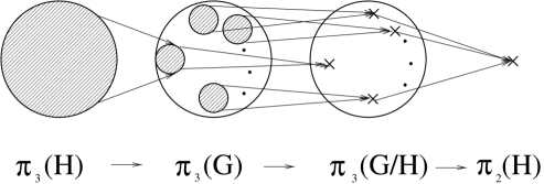
Figure 1: The exact homotopic sequence of (2.16) for simple groups if the index of embedding is greater than one.

In order the establish the relation (2.15) between the index of embedding and $\pi_{3}(G/H)$, we consider the following part of the exact homotopic sequence:

$$\ldots\to\pi_{3}(H)\to\pi_{3}(G)\to\pi_{3}(G/H)\to\pi_{2}(H)\to\ldots$$ (2.16)

Since this sequence is exact, ${\rm Im}\,f_{i}={\rm Ker}\,f_{i+1}$, where the $f$’s denote the maps in (2.16). We know that $\pi_{2}(H)=0$ for any Lie groups, while with the assumption that $G$ and $H$ are simple groups, $\pi_{3}(G)=\pi_{3}(H)=Z$. Thus we find that the sequence

$$Z\to Z\to\pi_{3}(G/H)\to 0$$ (2.17)

is exact. Since $\pi_{2}(H)=0$ the kernel of the map from $\pi_{3}(G/H)$ to $\pi_{2}(H)$ is the full $\pi_{3}(G/H)$. Due to the exact sequence, this means that the image of the map from $\pi_{3}(G)$ to $\pi_{3}(G/H)$ is again the full $\pi_{3}(G/H)$, ${\rm Im}(\pi_{3}(G))=\pi_{3}(G/H)$, where ${\rm Im}(\pi_{3}(G))$ denotes the image of $\pi_{3}(G)$. Therefore, $\pi_{3}(G/H)=\pi_{3}(G)/{\rm Ker}(\pi_{3}(G))$, where ${\rm Ker}(\pi_{3}(G))$ is the kernel of the map from $\pi_{3}(G)$ to $\pi_{3}(G/H)$. However, due to the first part of the exact sequence ${\rm Ker}(\pi_{3}(G))={\rm Im}(\pi_{3}(H))$. Thus we can conclude that

$$\pi_{3}(G/H)=\pi_{3}(G)/\mbox{Im}(\pi_{3}(H)),$$ (2.18)

where $\mbox{Im}(\pi_{3}(H))\subset\pi_{3}(G)$ is the image of $\pi_{3}(H)$. Next we want to use the information that the index of embedding is $\alpha$ in order to relate $\pi_{3}(G)$ and $\mbox{Im}(\pi_{3}(H))$. We have seen in Section 2.2 that the fact that the index of embedding is $\alpha$ combined with the Atiyah-Singer index theorem implies that the one instanton of $H$ corresponds to an $\alpha$ instanton of $G$. This means that winding around once in the $H$ subgroup corresponds to winding around $\alpha$-times in the full $G$ group. Since the value of $\pi_{3}$ measures how many times a given configuration is winding around the sphere at infinity, the above relation implies that

$$\mbox{Im}(\pi_{3}(H))=\alpha\times\pi_{3}(G),$$ (2.19)

A more precise argument for (2.19) is presented in Appendix A. Combining the facts that

$$\pi_{3}(G/H)=\pi_{3}(G)/\mbox{Im}(\pi_{3}(H)),$$

$$\mbox{Im}(\pi_{3}(H))=\alpha\times\pi_{3}(G),$$

$$\pi_{3}(G)=Z$$ (2.20)

immediately gives the desired relation

$$\pi_{3}(G/H)=Z_{\alpha}.$$ (2.21)

Fig. 1 illustrates the exact sequence for this case when $G$ and $H$ are both simple. Examples of non-trivial $\pi_{3}(G/H)$ include:

$$\pi_{3}(SU(N)/SO(N))=Z_{2},\;\;(N>3)$$

$$\pi_{3}(SU(3)/SO(3))=Z_{4},$$

$$\pi_{3}(Sp(2N)/SU(N))=Z_{2}.$$ (2.22)

The first two of these examples have been explicitly quoted in Ref. [33]. The case of the embedding of $SO(3)$ into $SU(3)$ (when the index $\alpha=4$) is illustrated in Fig. 2.

                                                                                                                     

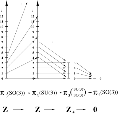
Figure 2: The exact homotopic sequence for the case that the index of embedding is four.

The physical meaning of (2.15) is that during the breaking of $G$ to $H$ the instantons get separated into two categories. Some instantons remain in the unbroken subgroup $H$, and are of the usual kind. However, there will be $Z_{\alpha}$ instantons in the partially broken group. Since these are $Z_{\alpha}$ and not $Z$-type instantons, it means that a combination of $\alpha$ of these instantons can unwind and be topologically trivial in $G/H$. This corresponds to the expectation that a collection of $\alpha$ of $Z_{\alpha}$ instantons will be ordinary instantons in $H$, and no longer in $G/H$.

In the case of $N=2$ theories, the low-energy $U(1)^{r}$ theory obtained after giving an expectation value to the adjoint does not contain instantons any more, thus as explained at the end of Section 2.1, one has to add the instanton corrections to the low-energy prepotential. This is expressed in the equation $\pi_{3}(G/U(1)^{r})=Z$, which tells us that all $G$ instantons are in the broken part of the gauge group, and thus their effects on the low-energy theory have to be added.

Let us now consider an example when $G$ is not a simple group. This is the case for example in the breaking $SO(4)\to SO(3)$, since $SO(4)\equiv(SU(2)\times SU(2))/Z_{2}$. To obtain $\pi_{3}(SO(4)/SO(3))$ we note that $SO(4)/SO(3)\simeq S^{3}$, which is a special case of the general relation $SO(N)/SO(N-1)\simeq S^{N-1}$. Since $\pi_{k}(S^{k})=Z$, we conclude that $\pi_{3}(SO(4)/SO(3))=Z$. This is again in accordance with our physics expectations, since we have seen, that during the breaking of $SU(2)\times SU(2)$ to the diagonal $SU(2)$ one particular combination of the one-instantons of the two $SU(2)$ factors (the $(1,1)$ instanton) will be mapped to the one-instanton of the diagonal $SU(2)$. Thus the complete tower of the other independent combination the instantons (the $(k,0)$ instantons for example) are missing from the diagonal $SU(2)$, and this is why $\pi_{3}(G/H)=Z$ now. Similarly, we find that for the general case of breaking $SU(N)\times SU(N)$ to the diagonal $SU(N)$ subgroup, $\pi_{3}((SU(N)\times SU(N))/SU(N))=Z$.

Thus we have seen that, during partial breaking of the gauge group, some of the original $G$ instantons may get mapped to $Z_{N}$ instantons in $G/H$. The effects of these instantons are no longer included in the low-energy effective theory based on the gauge group $H$. However, the effects of these $G/H$ instantons may leave non-trivial effects on the low-energy physics, and these have to be taken into account. In the remainder of this paper we will show several examples of the effects of these $Z_{N}$ instantons on the low-energy physics. We will see that in many cases, consistency of the low-energy theory will actually require the presence of these $Z_{N}$ instanton effects.

3 Examples of the Effects of $Z_{N}$ Instantons

In this section we present several examples of the effects of the $Z_{N}$ instantons discussed in the previous section on the low-energy effective theory. We will focus on supersymmetric theories, since the low-energy dynamics of these theories is much better understood than for general non-supersymmetric theories. Nevertheless, the arguments of the previous section do apply to the non-supersymmetric theories as well.

3.1 The $Z_{4}$ Instantons in $SU(3)\to SO(3)$

In this example we consider the $N=1$ duality of Pouliot and Strassler of $SO(8)$ with one spinor and $F$ vectors [13]. This theory is dual to $SU(F-4)$ with one symmetric tensor and $F$ antifundamental fields, and some gauge singlets. The duality is described in Table 1, where the superpotential of the dual $SU(F-4)$ theory is

$$W_{dual}=\alpha NSq^{2}+\beta T{\rm det}\,S,$$ (3.1)

where $\alpha$, $\beta$ are coupling constants. The operators are matched as $V^{i}V^{j}\leftrightarrow N^{ij}$, $p^{2}\leftrightarrow T$.

$$\begin{array}[]{c|cccc}&SO(8)&SU(F)&U(1)&U(1)_{R}\\ \hline\cr V&8_{v}&\raisebox{-0.5pt}{\hbox{\rule{0.4pt}{6.5pt}\hskip-0.4pt\rule{6.5pt}{0.4pt}\hskip-6.5pt\rule[6.5pt]{6.5pt}{0.4pt}}\rule[6.5pt]{0.4pt}{0.4pt}\hskip-0.4pt\rule{0.4pt}{6.5pt}}&-(F-4)&1-6/F\\ p&8_{s}&1&F(F-4)&1\\ \hline\cr\hline\cr&SU(F-4)&SU(F)&U(1)&U(1)_{R}\\ \hline\cr S&\raisebox{-0.5pt}{\hbox{\rule{0.4pt}{6.5pt}\hskip-0.4pt\rule{6.5pt}{0.4pt}\hskip-6.5pt\rule[6.5pt]{6.5pt}{0.4pt}}\rule[6.5pt]{0.4pt}{0.4pt}\hskip-0.4pt\rule{0.4pt}{6.5pt}}\hskip-0.4pt\raisebox{-0.5pt}{\hbox{\rule{0.4pt}{6.5pt}\hskip-0.4pt\rule{6.5pt}{0.4pt}\hskip-6.5pt\rule[6.5pt]{6.5pt}{0.4pt}}\rule[6.5pt]{0.4pt}{0.4pt}\hskip-0.4pt\rule{0.4pt}{6.5pt}}&1&-2F&0\\ q&\overline{\raisebox{-0.5pt}{\hbox{\rule{0.4pt}{6.5pt}\hskip-0.4pt\rule{6.5pt}{0.4pt}\hskip-6.5pt\rule[6.5pt]{6.5pt}{0.4pt}}\rule[6.5pt]{0.4pt}{0.4pt}\hskip-0.4pt\rule{0.4pt}{6.5pt}}}&\overline{\raisebox{-0.5pt}{\hbox{\rule{0.4pt}{6.5pt}\hskip-0.4pt\rule{6.5pt}{0.4pt}\hskip-6.5pt\rule[6.5pt]{6.5pt}{0.4pt}}\rule[6.5pt]{0.4pt}{0.4pt}\hskip-0.4pt\rule{0.4pt}{6.5pt}}}&2F-4&6/F\\ N&1&\raisebox{-0.5pt}{\hbox{\rule{0.4pt}{6.5pt}\hskip-0.4pt\rule{6.5pt}{0.4pt}\hskip-6.5pt\rule[6.5pt]{6.5pt}{0.4pt}}\rule[6.5pt]{0.4pt}{0.4pt}\hskip-0.4pt\rule{0.4pt}{6.5pt}}\hskip-0.4pt\raisebox{-0.5pt}{\hbox{\rule{0.4pt}{6.5pt}\hskip-0.4pt\rule{6.5pt}{0.4pt}\hskip-6.5pt\rule[6.5pt]{6.5pt}{0.4pt}}\rule[6.5pt]{0.4pt}{0.4pt}\hskip-0.4pt\rule{0.4pt}{6.5pt}}&-2(F-4)&2-12/F\\ T&1&1&2F(F-4)&2\end{array},$$

Table 1: The field content and symmetries of the electric $SO(8)$ theory and its magnetic dual $SU(F-4)$.

Integrating out the spinor $p$ of the electric theory with a mass term $\Delta W\propto p^{2}$ should reproduce the $SO$ duality of Ref. [7], since on the electric side we get an $SO(8)$ theory with $F$ vectors. On the magnetic side the mass of the spinor corresponds to a linear term in $T$ in the superpotential, which will become

$$W_{dual}=\alpha NSq^{2}+\beta T{\rm det}\,S+\gamma T,$$ (3.2)

with $\gamma$ a coupling constant. The $T$ equation of motion forces an expectation value to ${\rm det}\,S$, which breaks $SU(F-4)$ to $SO(F-4)$, while the $NSq^{2}$ term will turn into the $Nq^{2}$ superpotential of the $SO$ duality [13]. However, in the special case of $F=7$, the dual gauge group is $SO(3)$, and an additional superpotential term ${\rm det}\,N$ is needed for the $SO$ duality of Ref. [7]. This exactly happens when the breaking is $SU(3)\to SO(3)$, that is when the index of embedding is four. We will now show that the ${\rm det}\,N$ term in the superpotential required for duality is indeed generated by a $Z_{4}$ instanton effect.

For this we consider the two-instanton of $SU(3)$. This is one of the three instantons which is missing from the $SO(3)$ theory. The ’t Hooft effective Lagrangian for this two-instanton is given by

$$\tilde{S}^{10}\tilde{q}^{14}\lambda^{12}\Lambda^{6},$$ (3.3)

where $\tilde{S}$ is the fermionic component of the chiral superfield $S$, $\tilde{q}$ the fermion from $q$, $\lambda$ the gaugino, and $\Lambda^{6}$ is the two-instanton factor. The powers of these fields are fixed by the number of zero modes in the two-instanton background. In order to show that this will indeed result in a superpotential of the form ${\rm det}N$, we need to convert the fields in (3.3) to $\tilde{N}^{2}N^{5}$ for the case of $F=7$, since this is one of the contributions of the superpotential to the Lagrangian. Here $\tilde{N}$ is the fermionic component of $N$. In the presence of the expectation value $\langle S\rangle\propto(\gamma/\beta)^{1/3}$, the gaugino vertex $S^{*}\lambda\tilde{S}$ converts $\tilde{S}^{10}\lambda^{10}$ to ${\langle S\rangle^{*}}^{10}$. The integration over the instanton size will result in additional factors of $\langle S\rangle\langle S\rangle^{*}$. Since we are interested in a contribution to the superpotential, all dependence on $\langle S\rangle^{*}$ has to cancel after the integral over the instanton size is performed, due to the holomorphy of the superpotential. This can happen only if for every factor of $\langle S\rangle^{*}$ there is a $\langle S\rangle\langle S\rangle^{*}$ dividing the operator. Thus, every factor of $\langle S\rangle^{*}$ is converted to $\langle S\rangle^{-1}$, and so ${\langle S\rangle^{*}}^{10}$ has to be replaced by $\langle S\rangle^{-10}$ for the holomorphic part which can appear in the superpotential. The superpotential coupling $\alpha NSq^{2}$ converts ten $\tilde{q}$’s out of $\tilde{q}^{14}$ to $(\alpha N\langle S\rangle)^{5}$ by using the vertex $\alpha NS\tilde{q}^{2}$ five times, and the other four $\tilde{q}$’s together with the remaining two $\lambda$’s to the fermionic component of $(\alpha N\langle S\rangle)$ by using two $\tilde{q}\lambda q^{*}$ and two $\alpha Sq\tilde{N}\tilde{q}$ vertices. This is illustrated in Fig. 3. In total, the operator generated can be written in terms of the superpotential term

$$\frac{\mbox{det}\,(\alpha N\langle S\rangle)\Lambda^{6}}{\langle S\rangle^{10}}.$$ (3.4)

This form is consistent with all symmetries of the theory and has the right dimensionality to be a term in the superpotential. Up to a dimensionless constant $(\alpha\langle S\rangle)^{7}$, the superpotential can be rewritten as

$$\frac{{\rm det}\,N\,\Lambda^{6}}{\langle S\rangle^{10}}=\frac{{\rm det}\,N}{\tilde{\Lambda}^{4}},$$ (3.5)

where $\tilde{\Lambda}$ is the scale (Landau pole) of the $SO(3)$ theory. However, the one-loop $\beta$ function of the $SO(3)$ theory is $-8$, therefore the expression of (3.5) corresponds as expected to a “half-instanton” effect in the $SO(3)$ group, which can only be explained as a $Z_{4}$ instanton effect in the partially broken group.

                                                                                                                     

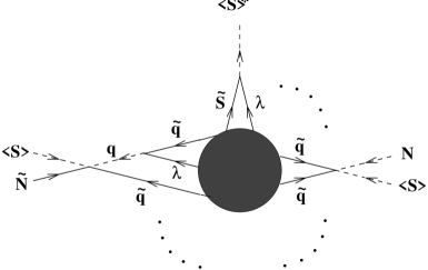
Figure 3: The contribution of the $Z_{4}$ instanton to the superpotential. The blob in the middle represents the two-instanton of $SU(3)$, which is one of the $Z_{4}$ instantons. The straight lines represent fermions while the dashed ones scalars. The fermionic lines emerging from the instanton form the ’t Hooft vertex. In addition, as explained in the text, several insertions of the scalar-fermion-gluino vertex and vertices from the superpotential $Nsq^{2}$ are needed to convert the ’t Hooft vertex into a superpotential contribution.

Thus one can see that the effect of one of the $Z_{4}$ instantons is to generate the superpotential term ${\rm det}N$. However, one needs to ask the question of why we took only the effect of the two instanton into account, and not those of the one and three instantons which are not present in the low-energy theory either. The absence of the effects of these instantons in the superpotential can be understood by considering the global charges of the theory. Consider the anomalous $R$-symmetry $U(1)_{X}$, under which $S$ and $q$ have charge zero (the fermionic components have charge $-1$), and the $SU(3)$ gauginos have charge $1$. In order for the superpotential (3.1) to carry charge $2$, $N$ and $T$ have to have $U(1)_{X}$ charge $2$. In addition, the non-anomalous $R$-charges can be read off from Table 1 for $F=7$. Thus the $R$-charges under these two symmetries are:

$$\begin{array}[]{|c|cccc|}\hline\cr&S&q&N&T\\ \hline\cr U(1)_{R}&0&6/7&2/7&2\\ U(1)_{X}&0&0&2&2\\ \hline\cr\end{array}$$

Note that both the $U(1)_{R}$ and $U(1)_{X}$ remain symmetries of the model at the classical level even with the added linear term $T$ in the superpotential. The ’t Hooft vertex of the one-instanton of $SU(3)$ is $\lambda^{6}\tilde{S}^{5}\tilde{q}^{7}$ which carries $U(1)_{X}$ charge $-6$ (and of course $U(1)_{R}$ charge zero). If this vertex is to come from a superpotential, then that superpotential term has to carry $U(1)_{X}$ charge $-4$ (and $U(1)_{R}$ charge $2$). Thus the difference between the $R$ and $X$ charge must be $6$. Below is a list of gauge and global invariants of the theory, of which the superpotential term must be constructed from:

$$\begin{array}[]{|c|ccc|}\hline\cr&U(1)_{R}&U(1)_{X}&R-X\\ \hline\cr{\rm det}S&0&0&0\\ T&2&2&0\\ {\rm det}(Sq^{2})&12&0&12\\ Nsq^{2}&2&2&0\\ {\rm det}N&2&14&12\\ \hline\cr\end{array}$$

One can see that the difference $R-X$ is either $\pm 12$ or $0$, thus $6$ can not be obtained in any way, therefore the 1-instantons (and similarly the 3-instantons) can not generate a superpotential term, but the 2-instanton can, as we have explicitly seen above.

In fact, the absence of the one-instanton effect is expected from the $SO(N)$ duality of the low-energy theories. Based on duality of the theories obtained after adding the spinor mass, we show below not only that there should not be any superpotential terms generated by the one (or three) instantons, but also that all effects of these instantons must decouple completely from the low-energy theory. This can be seen for arbitrary $F$ by considering the discrete symmetries of the theories. The original $SO(8)$ electric theory does not have a non-trivial discrete symmetry not contained in continuous symmetries, nor the magnetic $SU(3)$ theory. However after the spinor mass term is added, the electric theory flows to the $SO(8)$ theory with $F$ vectors, which has a $Z_{2F}\times{\cal P}$ discrete symmetry, where $Z_{2F}$ acts as $Q\to e^{i\pi/F}Q$ on the $SO(8)$ vectors, and ${\cal P}$ is the color conjugation type discrete symmetry, under which the sign of the first color is flipped (color parity) [14]. If duality is to hold, the low-energy $SO(3)$ theory has to have the same set of discrete symmetries. One discrete symmetry of the dual $SO(F-4)$ theory is obtained as the unbroken discrete subgroup of the original symmetries of the electric theory. Adding the term linear in $T$ to the superpotential breaks the ordinary global $U(1)$ to its $Z_{2F(F-4)}$ subgroup, under which the charges of $S,q,N$ and $T$ are $-2F,2F-4,-2(F-4)$ and $0$, respectively. However, the equation of motion for $T$ forces an expectation value to $S$, which would break this $Z_{2F(F-4)}$ symmetry further. To find the unbroken discrete symmetry, let us combine the action of the above $Z_{2F(F-4)}$ with a global $SU(F-4)$ gauge transformation $U$ of the form

$$U={\rm diag}(-e^{\pi i/(F-4)},e^{\pi i/(F-4)},\ldots,e^{\pi i/(F-4)}).$$

This is an element of $SU(F-4)$ since the determinant is one. Acting by this $U$ on $S$ as $S\to U^{T}SU$, and combining this with the action of the $Z_{2F(F-4)}$, $\langle S\rangle$ is left invariant. Thus this is an unbroken discrete global symmetry of the theory. Now let us determine how this symmetry acts on the $q$’s. The gauge transformation acts as $q\to U^{\dagger}q$, since $q$ is in a representation conjugate to $S$, while $q$ has charge $2F-4$ under the $Z_{2F(F-4)}$. Thus the action of this symmetry is given by

$$q\to{\rm diag}(-e^{-\pi i/(F-4)},e^{-\pi i/(F-4)},\ldots,e^{-\pi i/(F-4)})e^{\frac{\pi i(2F-4)}{F(F-4)}}q,$$

which is just

$$(q_{1},q_{2},\ldots,q_{F-4})\to e^{\pi i/F}(-q_{1},q_{2},\ldots,q_{F-4}).$$

One can see that this $Z_{2F}$ discrete symmetry is nothing but the combination of the $Z_{2F}$ symmetry which acts as $q\to e^{\pi i/F}q$ with the color-parity transformation ${\cal P}$. This is the discrete symmetry in the magnetic theory which is mapped to the $Z_{2F}$ symmetry of the electric theory. However, the color-parity ${\cal P}$ itself does not arise from the original symmetries of the $SU(F-4)$ theory, but it is an accidental symmetry of the low-energy effective theory. The ’t Hooft one-instanton vertex is invariant under the combination of $Z_{2F}{\cal P}$, since it is invariant under every global and gauge symmetry of the theory. However, as explained above ${\cal P}$ is not part of the symmetries of the original $SU(F-4)$ theory, and the ’t Hooft one-instanton vertex is not necessarily invariant under it. Indeed, since the one-instanton vertex contains exactly one $SU(F-4)$ epsilon-tensor, it changes sign under ${\cal P}$ and is thus not invariant, and the effects of this vertex would violate the ${\cal P}$ symmetry. However, by duality we expect that ${\cal P}$ itself is a good symmetry of the low-energy effective $SO(F-4)$ theory, therefore all effects of the one-instanton (which would break this symmetry) must decouple from the low-energy effective theory.

3.2 The $Z_{2}$ Instanton in $N=2$ $Sp(2N)\to SU(N)$

In this example we consider pure $N=2$ $Sp(2N)$ theories. This theory is in the Coulomb phase, and the low-energy effective action can be obtained from the following hyperelliptic Seiberg-Witten curve [19]:

$$y^{2}=x\prod_{i=1}^{N}(x-\Phi_{i}^{2})^{2}+4x\prod_{i=1}^{N}(x-\Phi_{i}^{2})\Lambda_{Sp}^{2N+2},$$ (3.6)

where $x$ and $y$ are the coordinates of the Seiberg-Witten curve, $\Lambda_{Sp}$ is the dynamical scale of the $Sp(2N)$ theory and $\Phi_{i}$ are the eigenvalues of the adjoint (symmetric tensor) of the $Sp(2N)$. We will show that by higgsing to the $SU(N)$ subgroup one obtains a curve that is different from the usual $SU(N)$ Seiberg-Witten curve. We will see explicitly that the effect of the $Z_{2}$ instanton is a shift in the Seiberg-Witten curve which modifies the singular locus of the curve.

Let us consider the breaking of the $Sp(2N)$ theory to its $U(N)$ subgroup. This is achieved by giving an expectation value $\Phi_{i}=V$ to the adjoint of $Sp(2N)$. This embedding has index two, thus there are potential effects of the $Z_{2}$ instanton on the low-energy effective theory. Writing $\Phi_{i}=V+\tilde{\Phi}_{i}/2$ in (3.6) and redefining $x$ as $x-V^{2}=Vx^{\prime}$ we get

$$y^{2}=(Vx^{\prime}+V^{2})^{2}\prod_{i=1}^{N}\left[V^{2}(x^{\prime}-\tilde{\Phi}_{i}-\frac{\tilde{\Phi}_{i}^{2}}{4V})^{2}\right]+4(Vx^{\prime}+V^{2})\Lambda_{Sp}^{2N+2}\prod_{i=1}^{N}\left[V(x^{\prime}-\tilde{\Phi}_{i}-\frac{\tilde{\Phi}_{i}^{2}}{4V})\right].$$

Taking the $V\to\infty$ limit and dropping the prime from $x$ and the tilde from $\Phi$, we obtain the curve

$$y^{2}=V^{2N+4}\prod_{i=1}^{N}(x-\Phi_{i})^{2}+4V^{N+2}\Lambda^{2N+2}_{Sp}\prod_{i=1}^{N}(x-\Phi_{i}).$$ (3.8)

The scale matching relation according to (2.11) is given by

$$(\Lambda_{Sp}^{2N+2})^{2}=\Lambda_{SU}^{2N}V^{2N+4}.$$ (3.9)

Thus after rescaling $y$, we finally obtain the following curve:

$$y^{2}=\left(\prod_{i=1}^{N}(x-\Phi_{i})^{2}+2\Lambda_{SU}^{N}\right)^{2}-4\Lambda_{SU}^{2N}.$$ (3.10)

This results needs more explanation. We can see that, except for the shift of the gauge-invariant polynomial $\prod_{i=1}^{N}\Phi_{i}$ by $2\Lambda_{SU}^{N}$, we have obtained the usual Seiberg-Witten curve for pure $N=2$ $SU(N)$ theories. This shift is proportional to $\Lambda_{SU}^{N}$, which is the square root of the one instanton factor of $SU(N)$, therefore can not be due to an instanton effect in the $SU(N)$ theory. Instead, this shift of the curve should be interpreted as the effect of the $Z_{2}$ instanton on the low-energy effective theory. Thus even in the $V\to\infty$ limit the effects of the $Z_{2}$ instanton do not decouple from the low-energy theory effective theory; it “remembers” that it has been obtained by higgsing from the $Sp(2N)$ theory. One can easily see that the two curves are not equivalent by comparing the discriminant of the curve in (3.10) to the discriminant of the usual $SU(N)$ curve. For example, the curve of (3.10) obtained by higgsing $Sp(4)$ to $SU(2)$ is given explicitly by

$$y^{2}=\left(x^{2}-u-2\Lambda_{SU}^{2}\right)^{2}-4\Lambda_{SU}^{4},$$ (3.11)

while the curve for the pure $N=2$ $SU(2)$ theory is given by

$$y^{2}=(x^{2}-u)^{2}-4\Lambda_{SU}^{4}.$$ (3.12)

In the usual $SU(2)$ theory the singularities occur at $u=\pm 2\Lambda_{SU}^{2}$, in the theory given by the curve of (3.11) the singularities occur at $u=0,-4\Lambda_{SU}^{2}$. One may ask the question of whether this shift in the curve (and in the position of the singularity) is a physically observable effect. From the purely low-energy point of view one could argue that this shift just amounts to a redefinition of the coordinates on the moduli space, and therefore in the strict low-energy limit this effect is unobservable. However, if one considers not only the low-energy effective theory but also the high-energy theories, effect of the shift is actually physically observable. One way of seeing this is to remember that the $SU(N)$ theory has a non-anomalous $Z_{2N}$ discrete symmetry, under which the adjoint field has charge one, thus $u$ of the above example carries charge two. We have seen that the singularity occurs at non-zero values of $u$ in the pure $N=2$ $SU(2)$ theory, thus breaking the discrete symmetry. However, in the $SU(2)$ theory obtained from higgsing the $Sp(4)$ the effects of the $Z_{2}$ instanton shift one of the singularities to zero. Thus in this effective $SU(2)$ theory the discrete symmetry is not broken at one of the singularities. The coexistence of the unbroken discrete symmetry and the massless monopole is the effect of the $G/H$ instantons.

One can discuss the same issue from a different point of view. Consider the pure $N=2$ $SU(2)$ theory as a high-energy theory. This theory has an anomalous $U(1)_{R}$ symmetry, which can be used to obtain selection rules if one assigns an appropriate charge to the dynamical scale $\Lambda_{SU}^{4}$ of the theory. Requiring invariance under this symmetry will tell us what kind of redefinitions of the moduli space parameter $u$ are possible. Since the shift in $u$ required to connect the two curves in (3.11) and (3.12) would be proportional to the square root of the instanton factor $\Lambda_{SU}^{4}$, this would signal that the $U(1)_{R}$ symmetry is broken, therefore such a shift is not allowed by the anomalous $U(1)_{R}$ symmetry. Thus taking into account the symmetries of the high-energy theory distinguishes between the two curves presented above. We will see in the following section the same effect again in the case of $SO(N)$ theory, where the shift in the curve changes the fact whether some non-anomalous continuous global symmetries of the high-energy theory are preserved at the singularity or not.

3.3 The $Z$ Instantons in $SU(N)\times SU(N)\to SU(N)_{D}$

In this section we will consider examples very similar to the $N=2$ theory presented in the previous section. Here we consider $N=1$ product group theories in the Coulomb phase [21, 22]. Let us consider first the $SU(2)\times SU(2)$ model of Ref. [21]. The matter content is given by

$$\begin{array}[]{c|cc}&SU(2)&SU(2)\\ \hline\cr Q_{1}&\raisebox{-0.5pt}{\hbox{\rule{0.4pt}{6.5pt}\hskip-0.4pt\rule{6.5pt}{0.4pt}\hskip-6.5pt\rule[6.5pt]{6.5pt}{0.4pt}}\rule[6.5pt]{0.4pt}{0.4pt}\hskip-0.4pt\rule{0.4pt}{6.5pt}}&\raisebox{-0.5pt}{\hbox{\rule{0.4pt}{6.5pt}\hskip-0.4pt\rule{6.5pt}{0.4pt}\hskip-6.5pt\rule[6.5pt]{6.5pt}{0.4pt}}\rule[6.5pt]{0.4pt}{0.4pt}\hskip-0.4pt\rule{0.4pt}{6.5pt}}\\ Q_{2}&\raisebox{-0.5pt}{\hbox{\rule{0.4pt}{6.5pt}\hskip-0.4pt\rule{6.5pt}{0.4pt}\hskip-6.5pt\rule[6.5pt]{6.5pt}{0.4pt}}\rule[6.5pt]{0.4pt}{0.4pt}\hskip-0.4pt\rule{0.4pt}{6.5pt}}&\raisebox{-0.5pt}{\hbox{\rule{0.4pt}{6.5pt}\hskip-0.4pt\rule{6.5pt}{0.4pt}\hskip-6.5pt\rule[6.5pt]{6.5pt}{0.4pt}}\rule[6.5pt]{0.4pt}{0.4pt}\hskip-0.4pt\rule{0.4pt}{6.5pt}}\end{array}.$$

This theory is in the Coulomb phase, and the Seiberg-Witten curve is given by

$$y^{2}=(x^{2}-(u-\Lambda_{1}^{4}-\Lambda_{2}^{4}))^{2}-4\Lambda_{1}^{4}\Lambda_{2}^{4},$$ (3.13)

where $u={\rm det}\,M$, $M_{ij}=Q_{i}Q_{j}$, and the $\Lambda_{1,2}$ are the dynamical scales of the two $SU(2)$ factors. Let us give an expectation value to $Q_{1}$, thereby breaking $SU(2)\times SU(2)$ to the diagonal $SU(2)$ subgroup. We have seen in Section 2.4 that there are potential $G/H$ instantons appearing in this embedding which might have an effect on the low-energy theory. To find their effect on the low-energy theory we write $M_{11}=V^{2}$, and the scale matching relation $\Lambda_{D}^{4}=\frac{\Lambda_{1}^{4}\Lambda_{2}^{4}}{V^{4}}$. Denote the ratio of the two $SU(2)$ scales $\frac{\Lambda_{1}^{4}}{\Lambda_{2}^{4}}=k^{2}$. Then the low-energy curve can be written as

$$y^{2}=(x^{2}-V^{2}(u_{D}-(k+k^{-1})\Lambda_{D}^{2}))^{2}-4\Lambda_{D}^{4}V^{4}.$$ (3.14)

After an appropriate rescaling of $x$ and $y$ the curve becomes

$$y^{2}=(x^{2}-(u_{D}-(k+k^{-1})\Lambda_{D}^{2}))^{2}-4\Lambda_{D}^{4}.$$ (3.15)

The conclusion is similar as in the previous example. The Seiberg-Witten curve differs from the ordinary $SU(2)$ curve, and contains effects which can not be explained by instanton effects in the diagonal $SU(2)$ theory. Instead they are due to the $G/H$ instantons. Note that here the low-energy theory depends also on the ratio of the scales of the original two $SU(2)$ groups, which is not lost in the effective $SU(2)$ curve exactly due to the effects of the $G/H$ instantons. Note that for $k=1$, that is in the case when the two scales of the original $SU(2)$ theories coincide, the location of one of the singularities is shifted to the origin of the moduli space. This changes the monodromies, and implies that additional monopoles must become massless at this point. Thus one can see that the shift in the curve, which is an effect of the instantons in the broken part of the gauge group, encodes important physical information.

It is straightforward to generalize this example to the general $SU(N)\times SU(N)$ theories of Ref. [22], which we will briefly review at the end of this section. First, however, let us examine the $SO(N)$ theory with $N-2$ vectors discussed in Ref. [7], which is very closely related to the $SU(2)\times SU(2)$ theory analyzed above. This theory is again in the Coulomb phase, and the Seiberg-Witten curve is given by

$$y^{2}=\left[x^{2}-(U-2\Lambda_{SO}^{2N-4})\right]-4\Lambda_{SO}^{4N-8},$$ (3.16)

where $U={\rm det}\,M$, $M$ is the meson matrix $M_{ij}=Q_{i}Q_{j}$, $i=1,\ldots,N-2$, and $\Lambda_{SO}$ is the dynamical scale of the $SO(N)$ theory. At the origin of the moduli space $M_{ij}=0$ the $SU(N-2)$ global symmetry arising from rotations of the $N-2$ vectors is unbroken, and the ’t Hooft anomaly matching conditions have to be satisfied. One finds that this is indeed the case, once we realize that the curve (3.16) has a singularity at the origin, and $N-2$ monopoles transforming as an antifundamental representation under the $SU(N-2)$ global symmetry become massless. Thus one can see that the fact that one of the singularities is precisely at the origin plays a crucial physical role. Let us now examine how this singularity at the origin arises. In order to obtain the curve of (3.16) one breaks the $SO(N)$ theory to an $SO(4)\sim SU(2)\times SU(2)$ theory by giving an expectation value to $N-4$ vectors. This way one obtains an $SU(2)\times SU(2)$ theory with exactly the same matter content as discussed above, and the two scales equal, thus $k=1$. Further breaking to the diagonal $SU(2)$ subgroup as discussed above will determine the curve (3.16) uniquely. The shift of the $SU(2)$ curve due to the effects of the $G/H$ instantons will result in the shift $2\Lambda_{SO}^{2N-4}$ in the curve for the $SO(N)$ theory. This shift, as explained above, is crucial for the ’t Hooft anomaly matching, and is, in the low-energy $SU(2)$ theory, due to the effects of the $G/H$ instantons.

We close this section by explaining how to generalize the results for the $SU(2)\times SU(2)$ theory presented at the beginning of this section to $SU(N)\times SU(N)$. The matter content of the theories we consider is given by

$$\begin{array}[]{c|cc}&SU(N)&SU(N)\\ \hline\cr Q_{1}&\raisebox{-0.5pt}{\hbox{\rule{0.4pt}{6.5pt}\hskip-0.4pt\rule{6.5pt}{0.4pt}\hskip-6.5pt\rule[6.5pt]{6.5pt}{0.4pt}}\rule[6.5pt]{0.4pt}{0.4pt}\hskip-0.4pt\rule{0.4pt}{6.5pt}}&\overline{\raisebox{-0.5pt}{\hbox{\rule{0.4pt}{6.5pt}\hskip-0.4pt\rule{6.5pt}{0.4pt}\hskip-6.5pt\rule[6.5pt]{6.5pt}{0.4pt}}\rule[6.5pt]{0.4pt}{0.4pt}\hskip-0.4pt\rule{0.4pt}{6.5pt}}}\\ Q_{2}&\overline{\raisebox{-0.5pt}{\hbox{\rule{0.4pt}{6.5pt}\hskip-0.4pt\rule{6.5pt}{0.4pt}\hskip-6.5pt\rule[6.5pt]{6.5pt}{0.4pt}}\rule[6.5pt]{0.4pt}{0.4pt}\hskip-0.4pt\rule{0.4pt}{6.5pt}}}&\raisebox{-0.5pt}{\hbox{\rule{0.4pt}{6.5pt}\hskip-0.4pt\rule{6.5pt}{0.4pt}\hskip-6.5pt\rule[6.5pt]{6.5pt}{0.4pt}}\rule[6.5pt]{0.4pt}{0.4pt}\hskip-0.4pt\rule{0.4pt}{6.5pt}}\end{array}.$$

This theory is in the Coulomb phase, with $N-1$ unbroken $U(1)$ factors at the generic point of the moduli space. The Seiberg-Witten curve for this theory has been determined in Ref. [22]. The independent gauge invariant operators are $B_{1}={\rm det}Q_{1}$, $B_{2}={\rm det}Q_{2}$, $T_{n}={\rm Tr}(Q_{1}Q_{2})^{n}$, $n=1,\ldots,N-1$. The Seiberg-Witten curve for this theory is

$$y^{2}=\left(\sum_{i=0}^{N}s_{i}x^{N-i}+(-1)^{N}(\Lambda_{1}^{2N}+\Lambda_{2}^{2N})\right)^{2}-4\Lambda_{1}^{2N}\Lambda_{2}^{2N},$$ (3.17)

where the $s_{i}$ are related to the $u_{k}$’s by Newton’s formula

$$ks_{k}+\sum_{j=1}^{k}js_{k-j}u_{j}=0,$$ (3.18)

$s_{0}=1,s_{1}=u_{1}=0$, and the operators $u_{k}$ are the invariants of the “composite adjoint” $\Phi=Q_{1}Q_{2}-\frac{1}{N}{\rm Tr}Q_{1}Q_{2}$, $u_{k}=\frac{1}{k}{\rm Tr}\Phi^{k}$, and are to be expressed in terms of the gauge invariants $T_{i}$ and $B_{i}$ via classical expressions (for example for the case of $SU(3)\times SU(3)$ $u_{2}=\frac{1}{2}(T_{2}-\frac{1}{3}T_{1}^{2}),u_{3}=\frac{1}{3}(3B_{1}B_{2}+\frac{1}{2}T_{2}T_{1}-\frac{5}{18}T_{1}^{3})$).

Now consider breaking $SU(N)\times SU(N)$ to the diagonal $SU(N)_{D}$ subgroup, by the expectation value

$$Q_{1}=v\left(\begin{array}[]{cccc}1\\ &1\\ &&\ddots\\ &&&1\end{array}\right),$$ (3.23)

that is by giving a VEV to $B_{1}$ and no other operator. The matching of scales is given by $\frac{\Lambda_{1}^{2N}\Lambda_{2}^{2N}}{v^{2N}}=\Lambda_{D}^{2N}$, while the operators $u_{k}$ will be matched to the invariants of the adjoint of the diagonal $SU(N)_{D}$ by $u_{k}^{D}=\frac{u_{k}}{v^{k}}$. Plugging these relations back into (3.17), and rescaling $x\to x/v$, $y\to y/v^{N}$, we obtain the curve for the $SU(N)_{D}$ theory:

$$y^{2}=\left(\sum_{i=0}^{N}s_{i}^{D}x^{N-i}+(-1)^{N}(k+\frac{1}{k})\Lambda_{D}^{N}\right)^{2}-4\Lambda_{D}^{2N},$$ (3.24)

where $k=\frac{\Lambda_{1}^{N}}{\Lambda_{2}^{N}}$, and $s_{i}^{D}$ are the symmetric variables for the diagonal group $s_{i}^{D}=\frac{s_{i}}{v^{i}}$. The conclusion is just like before: the Seiberg-Witten curve we obtain in this limit is almost identical to the usual $N=2$ Seiberg-Witten curve, but it differs from it by a shift due to the $G/H$ instantons in the broken part of the group. Again the relative sizes of the original scales $\Lambda_{1}$ and $\Lambda_{2}$ appear in the low-energy theory due to the $G/H$ instanton effects.

3.4 The $Z$ Instantons in $SO(4)\to SO(3)$

In this example we consider the breaking $SO(4)\to SO(3)$ by looking at the $N=1$ duality in $SO(N)$ groups with vectors discussed in Ref. [7]. The electric theory is

$$\begin{array}[]{c|cccc}&SO(N)&SU(F)&U(1)_{R}&Z_{2F}\\ \hline\cr Q&\raisebox{-0.5pt}{\hbox{\rule{0.4pt}{6.5pt}\hskip-0.4pt\rule{6.5pt}{0.4pt}\hskip-6.5pt\rule[6.5pt]{6.5pt}{0.4pt}}\rule[6.5pt]{0.4pt}{0.4pt}\hskip-0.4pt\rule{0.4pt}{6.5pt}}&\raisebox{-0.5pt}{\hbox{\rule{0.4pt}{6.5pt}\hskip-0.4pt\rule{6.5pt}{0.4pt}\hskip-6.5pt\rule[6.5pt]{6.5pt}{0.4pt}}\rule[6.5pt]{0.4pt}{0.4pt}\hskip-0.4pt\rule{0.4pt}{6.5pt}}&1-\frac{N-2}{F}&1\end{array},$$ (3.25)

while the dual is $SO(F-N+4)$ with $F$ vectors:

$$\begin{array}[]{c|cccc}&SO(F-N+4)&SU(F)&U(1)_{R}&Z_{2F}\\ \hline\cr q&\raisebox{-0.5pt}{\hbox{\rule{0.4pt}{6.5pt}\hskip-0.4pt\rule{6.5pt}{0.4pt}\hskip-6.5pt\rule[6.5pt]{6.5pt}{0.4pt}}\rule[6.5pt]{0.4pt}{0.4pt}\hskip-0.4pt\rule{0.4pt}{6.5pt}}&\overline{\raisebox{-0.5pt}{\hbox{\rule{0.4pt}{6.5pt}\hskip-0.4pt\rule{6.5pt}{0.4pt}\hskip-6.5pt\rule[6.5pt]{6.5pt}{0.4pt}}\rule[6.5pt]{0.4pt}{0.4pt}\hskip-0.4pt\rule{0.4pt}{6.5pt}}}&\frac{N-2}{F}&-1\\ M&1&\raisebox{-0.5pt}{\hbox{\rule{0.4pt}{6.5pt}\hskip-0.4pt\rule{6.5pt}{0.4pt}\hskip-6.5pt\rule[6.5pt]{6.5pt}{0.4pt}}\rule[6.5pt]{0.4pt}{0.4pt}\hskip-0.4pt\rule{0.4pt}{6.5pt}}\hskip-0.4pt\raisebox{-0.5pt}{\hbox{\rule{0.4pt}{6.5pt}\hskip-0.4pt\rule{6.5pt}{0.4pt}\hskip-6.5pt\rule[6.5pt]{6.5pt}{0.4pt}}\rule[6.5pt]{0.4pt}{0.4pt}\hskip-0.4pt\rule{0.4pt}{6.5pt}}&2-2\frac{N-2}{F}&2\end{array},$$ (3.26)

and a superpotential $Mq^{2}$, where the $q$’s are the magnetic quarks and $M$ are the mesons. However, in the case of $F=N-1$, the dual is $SO(3)$ with $F$ vectors, but the superpotential includes an additional term $W=Mq^{2}+{\rm det}M$. This ${\rm det}M$ term is present in the dual superpotential only for $F=N-1$. This prompts the question of how this ${\rm det}M$ term is generated if one starts from the duality for $F=N$ and integrate out one flavor. Thus we consider $SO(N)$ with $N$ vectors and no superpotential. The dual is $SO(4)$ with $F$ vectors $q$, a gauge singlet meson $M$ and a superpotential $Mq^{2}$. Adding a mass term for one vector of the electric theory results in an $SO(N)$ electric theory with $N-1$ vectors. On the dual side the mass term corresponds to adding a term linear in the meson field to the superpotential. Thus the full superpotential is $W=Mq^{2}+mM_{N,N}$. The equation of motion with respect to $M_{N,N}$ forces an expectation value to one of the dual quarks higgsing the dual gauge group from $SO(4)$ to $SO(3)$. Thus we get the non-trivial embedding of $SO(3)$ into $SO(4)$, that is $SU(2)_{D}$ into $SU(2)\times SU(2)$. The effect of this is that some of the instantons which are in the broken part of the group are no longer included in the low-energy theory. The effects of these instantons will be exactly to reproduce the superpotential term ${\rm det}M$ required by duality.

We describe how this term is generated by the instantons in the broken group. The $(1,0)$ instanton configuration in the first $SU(2)$ factor of $SO(4)\simeq(SU(2)_{L}\times SU(2)_{R})/Z_{2}$ generates the ’t Hooft operator

$$\tilde{q}^{1}\tilde{q}^{1}\cdots\tilde{q}^{N}\tilde{q}^{N}\lambda^{4}\Lambda_{L}^{6-2N},$$ (3.27)

where $\lambda$ is the gaugino in the first $SU(2)$ factor and $\Lambda_{L}$ is the scale of the first $SU(2)$ factor. In the presence of the expectation value $\langle q^{N}\rangle\neq 0$, both $\tilde{q}^{N}$’s in (3.27) are contracted with the gauginos $\lambda$ to become ${q^{N}}^{*}$. As explained in Section 3.1, after the integral over the instanton size, a factor of $1/|\langle q^{N}\rangle|^{4}$ appears and the dependence on ${q^{N}}^{*}$ is canceled, and a factor of $1/\langle q^{N}\rangle^{2}$ remains. All the other $\tilde{q}^{i}$’s are contracted using the superpotential coupling $\hat{M}_{ij}q^{i}q^{j}$, where $\hat{M}$ is the submatrix of $M$ with $N$-th row and column removed, and become $\mbox{det}\,\hat{M}$ (four of them are combined with the remaining two $\lambda$’s to give fermionic component of $\hat{M}_{ij}$). The end result is the superpotential

$$\frac{(\mbox{det}\,\hat{M})\Lambda_{L}^{6-N}}{\langle q^{N}\rangle^{2}},$$ (3.28)

which is the term $\mbox{det}\,\hat{M}$ required for duality. Exactly the same superpotential is generated from the $(0,1)$ instanton configuration except for the replacement of $\Lambda_{L}$ by $\Lambda_{R}$.

An alternative way of obtaining the same superpotential term is to reduce the problem of that of $SU(2)\times SU(2)$ with one representation in $(\raisebox{-0.5pt}{\hbox{\rule{0.4pt}{6.5pt}\hskip-0.4pt\rule{6.5pt}{0.4pt}\hskip-6.5pt\rule[6.5pt]{6.5pt}{0.4pt}}\rule[6.5pt]{0.4pt}{0.4pt}\hskip-0.4pt\rule{0.4pt}{6.5pt}},\raisebox{-0.5pt}{\hbox{\rule{0.4pt}{6.5pt}\hskip-0.4pt\rule{6.5pt}{0.4pt}\hskip-6.5pt\rule[6.5pt]{6.5pt}{0.4pt}}\rule[6.5pt]{0.4pt}{0.4pt}\hskip-0.4pt\rule{0.4pt}{6.5pt}})$. The instanton corrections in this theory have been analyzed in Ref. [8], therefore this method will result in the superpotential term including the appropriate coefficient. Below we briefly repeat this argument of Ref. [7] as well. Consider the point on the moduli space of the dual $SO(4)$ theory where the meson has an expectation value of rank $N-1$. This gives mass to all but one of the dual quarks $q$. On this point instantons (which will later exactly correspond to instantons in the broken part of the $SO(4)$) generate a superpotential

$$W_{inst}=2\frac{\tilde{\Lambda}_{L}^{5}+\tilde{\Lambda}_{R}^{5}}{q^{N}q^{N}},$$ (3.29)

where $q^{N}$ is the only massless flavor and the $\tilde{\Lambda}_{L,R}$ are the scales of the effective $SU(2)_{L}\times SU(2)_{R}$ theory after the $N-1$ flavors have been integrated out. The matching of scales relates them to the original scale of the $SO(4)$ theory by $\tilde{\Lambda}_{L,R}^{5}\propto{\rm det}\hat{M}\Lambda_{L,R}^{6-N}$. After the mass to the last flavor has been added, $q^{N}$ will get an expectation value, and the due to the matching relation the superpotential of (3.29) will be exactly the ${\rm det}M$ term required by duality.

3.5 The $Z_{2}$ Instanton in $N=1$ $Sp(2N)\to SU(N)$

In this example we will consider $N=1$ supersymmetric $Sp(2N)$ theories with a symmetric tensor (adjoint) and $2F$ fields in the fundamental representation, and a tree-level superpotential $W={\rm Tr}\,X^{2(k+1)}$. A duality for this theory has been described in Ref. [27] and is summarized in the table below.

$$\begin{array}[]{c|ccc}&Sp(2N)&SU(2F)&U(1)_{R}\\ \hline\cr X&\raisebox{-0.5pt}{\hbox{\rule{0.4pt}{6.5pt}\hskip-0.4pt\rule{6.5pt}{0.4pt}\hskip-6.5pt\rule[6.5pt]{6.5pt}{0.4pt}}\rule[6.5pt]{0.4pt}{0.4pt}\hskip-0.4pt\rule{0.4pt}{6.5pt}}\hskip-0.4pt\raisebox{-0.5pt}{\hbox{\rule{0.4pt}{6.5pt}\hskip-0.4pt\rule{6.5pt}{0.4pt}\hskip-6.5pt\rule[6.5pt]{6.5pt}{0.4pt}}\rule[6.5pt]{0.4pt}{0.4pt}\hskip-0.4pt\rule{0.4pt}{6.5pt}}&1&\frac{1}{k+1}\\ Q&\raisebox{-0.5pt}{\hbox{\rule{0.4pt}{6.5pt}\hskip-0.4pt\rule{6.5pt}{0.4pt}\hskip-6.5pt\rule[6.5pt]{6.5pt}{0.4pt}}\rule[6.5pt]{0.4pt}{0.4pt}\hskip-0.4pt\rule{0.4pt}{6.5pt}}&\raisebox{-0.5pt}{\hbox{\rule{0.4pt}{6.5pt}\hskip-0.4pt\rule{6.5pt}{0.4pt}\hskip-6.5pt\rule[6.5pt]{6.5pt}{0.4pt}}\rule[6.5pt]{0.4pt}{0.4pt}\hskip-0.4pt\rule{0.4pt}{6.5pt}}&1-\frac{N+1}{F(k+1)}\\ \hline\cr\hline\cr&Sp(2\tilde{N})&SU(2F)&U(1)_{R}\\ \hline\cr Y&\raisebox{-0.5pt}{\hbox{\rule{0.4pt}{6.5pt}\hskip-0.4pt\rule{6.5pt}{0.4pt}\hskip-6.5pt\rule[6.5pt]{6.5pt}{0.4pt}}\rule[6.5pt]{0.4pt}{0.4pt}\hskip-0.4pt\rule{0.4pt}{6.5pt}}\hskip-0.4pt\raisebox{-0.5pt}{\hbox{\rule{0.4pt}{6.5pt}\hskip-0.4pt\rule{6.5pt}{0.4pt}\hskip-6.5pt\rule[6.5pt]{6.5pt}{0.4pt}}\rule[6.5pt]{0.4pt}{0.4pt}\hskip-0.4pt\rule{0.4pt}{6.5pt}}&1&\frac{1}{k+1}\\ q&\raisebox{-0.5pt}{\hbox{\rule{0.4pt}{6.5pt}\hskip-0.4pt\rule{6.5pt}{0.4pt}\hskip-6.5pt\rule[6.5pt]{6.5pt}{0.4pt}}\rule[6.5pt]{0.4pt}{0.4pt}\hskip-0.4pt\rule{0.4pt}{6.5pt}}&\overline{\raisebox{-0.5pt}{\hbox{\rule{0.4pt}{6.5pt}\hskip-0.4pt\rule{6.5pt}{0.4pt}\hskip-6.5pt\rule[6.5pt]{6.5pt}{0.4pt}}\rule[6.5pt]{0.4pt}{0.4pt}\hskip-0.4pt\rule{0.4pt}{6.5pt}}}&1-\frac{\tilde{N}+1}{F(k+1)}\\ M_{2n}&1&\raisebox{-3.5pt}{\hbox{\rule{0.4pt}{6.5pt}\hskip-0.4pt\rule{6.5pt}{0.4pt}\hskip-6.5pt\rule[6.5pt]{6.5pt}{0.4pt}}\rule[6.5pt]{0.4pt}{0.4pt}\hskip-0.4pt\rule{0.4pt}{6.5pt}}\hskip-6.9pt\raisebox{3.0pt}{\hbox{\rule{0.4pt}{6.5pt}\hskip-0.4pt\rule{6.5pt}{0.4pt}\hskip-6.5pt\rule[6.5pt]{6.5pt}{0.4pt}}\rule[6.5pt]{0.4pt}{0.4pt}\hskip-0.4pt\rule{0.4pt}{6.5pt}}&2-\frac{2(N+1)-2nF}{F(k+1)}\\ M_{2m+1}&1&\raisebox{-0.5pt}{\hbox{\rule{0.4pt}{6.5pt}\hskip-0.4pt\rule{6.5pt}{0.4pt}\hskip-6.5pt\rule[6.5pt]{6.5pt}{0.4pt}}\rule[6.5pt]{0.4pt}{0.4pt}\hskip-0.4pt\rule{0.4pt}{6.5pt}}\hskip-0.4pt\raisebox{-0.5pt}{\hbox{\rule{0.4pt}{6.5pt}\hskip-0.4pt\rule{6.5pt}{0.4pt}\hskip-6.5pt\rule[6.5pt]{6.5pt}{0.4pt}}\rule[6.5pt]{0.4pt}{0.4pt}\hskip-0.4pt\rule{0.4pt}{6.5pt}}&2-\frac{2(N+1)-(2m+1)F}{F(k+1)}\end{array}$$

Here $\tilde{N}=(2k+1)F-N-2$, and $n=0,\ldots,k$, $m=0,\ldots,k-1$. The superpotential of the magnetic theory is

$$W_{magn}=\alpha{\rm Tr}\,Y^{2(k+1)}+\sum_{n=0}^{2k}\beta_{n}M_{n}qY^{2k-n}q,$$ (3.30)

where $\alpha$, $\beta_{n}$ are coupling constants. Now let us perturb this theory by adding a mass term ${\rm Tr}\,X^{2}$ to the $Sp(2N)$ adjoint of the electric theory. This will break the $Sp$ group and make all components of the adjoint massive. With this superpotential one can have different patterns of symmetry breaking in the electric theory, which are non-trivially mapped to the symmetry breaking in the magnetic theory. As described in Ref. [27], the expectation value for $X$ which has $p_{0}$ zero eigenvalues and $p_{l}$ eigenvalues $x_{l}$ breaks the electric $Sp(2N)$ theory to $Sp(2p_{0})\times U(p_{1})\times\ldots U(p_{k})$, where $\sum_{j=0}^{k}p_{j}=N$. The magnetic $Sp(2\tilde{N})$ group is broken by the corresponding superpotential $\gamma{\rm Tr}\,Y^{2}$ to $Sp(2(F-p_{0}-2))\times U(2F-p_{1})\times\ldots\times U(2F-p_{k})$. Since we are interested in the case when $Sp(2\tilde{N})\to U(\tilde{N})$, we choose the values $p_{0}=F-2$, $p_{1}=2F-\tilde{N}$ and all other $p_{i}=2F$. This way the magnetic theory after the breaking becomes an $U(\tilde{N})$ theory, and since the index of embedding is two, there are potential $Z_{2}$ instanton effects in this breaking. On the electric side with the above values of $p_{i}$ we find an $Sp(2F-4)\times U(2F-\tilde{N})\times U(2F)\times\ldots\times U(2F)$ theory, where the $Sp(2F-4)$ has $2F$ fundamentals, and all unitary factors have $2F$ flavors. Since the $U(2F)$ factors have $2F$ flavors, they confine with a quantum deformed moduli space and no superpotential. The magnetic gauge group $U(\tilde{N})$ is just the dual of the $U(2F-\tilde{N})$ factors of the electric side, and the superpotential required for duality will be obtained from the superpotential of (3.30). However, the electric theory has an additional $Sp(2F-4)$ gauge group with $2F$ fundamentals, which is s-confining, that is there is a confining superpotential ${\rm Pf}\,M_{0}$ generated. What we want to investigate is how this term necessary to maintain duality is generated in the magnetic theory. We will see that this term is exactly generated by the $Z_{2}$ instanton.

For this we consider the one instanton effective Lagrangian term of the original $Sp(2\tilde{N})$ theory. This is given by

$$\tilde{q}^{2F}\tilde{Y}^{2\tilde{N}+2}\lambda^{2\tilde{N}+2}\Lambda^{2\tilde{N}+2-F},$$ (3.31)

where $\tilde{q}$ is the fermionic component of the dual quarks $q$, $\tilde{Y}$ is the fermionic component of the adjoint $Y$, and $\lambda$ is the gaugino. The exponents are obtained from counting the zero modes in the one instanton background. Now we show how these zero modes give rise to a superpotential coupling in the presence of the expectation value $\langle Y\rangle$. Two of the $\tilde{Y}$ are contracted with the mass term $\gamma$. The gaugino interaction $Y^{*}\lambda\tilde{Y}$ converts the rest of $\tilde{Y}$ together with $2\tilde{N}$ of gaugino fields to ${\langle Y\rangle^{*}}^{2\tilde{N}}$; just like in Section 3.1 this is equivalent to the holomorphic part $\langle Y\rangle^{-2\tilde{N}}$ which can appear in the superpotential. Using the superpotential coupling $\beta_{0}M_{0}q\langle Y\rangle^{2k}q$, all $\tilde{q}$ but four are contracted as $(\beta_{0}M_{0}\langle Y\rangle^{2k})^{2F-2}$. Two out of the remaining four $\tilde{q}$’s are contracted with the remaining two gauginos using the gaugino interaction vertex $q^{*}\lambda\tilde{q}$ to $q^{*}$. These scalars are finally contracted with the remaining two $\tilde{q}$’s using the superpotential coupling $\beta_{0}M_{0}q\langle Y\rangle^{2k}q$ to the fermionic component of $(\beta_{0}M_{0}\langle Y\rangle^{2k})$. Putting everything together, we obtain the superpotential term

$$\frac{\gamma\mbox{Pf}\,(\beta_{0}M_{0}\langle Y\rangle^{2k})\,\Lambda^{2\tilde{N}+2-F}}{\langle Y\rangle^{2\tilde{N}}}.$$ (3.32)

This term is consistent with all symmetries of the theory and has the right dimensionality as a superpotential term. Omitting dependences on the mass $\gamma$, the coupling $\beta_{0}$ and the expectation value $\langle Y\rangle$, this is indeed the form expected: $\mbox{Pf}\,M_{0}$.

4 Conclusions

We have investigated the question of when instantons in partially broken gauge groups can have effects on the low-energy effective gauge theory. We have seen that in some cases (when the embedding of the unbroken group $H$ into the original group $G$ is non-trivial) some of the instantons of the original group $G$ are missing in the low-energy theory. The effects of these $G/H$ instantons has to be considered and added to the low-energy effective theory. In the case when both $G$ and $H$ are simple groups, considering the index of embedding is sufficient to decide whether such instanton effects may exist or not. In the more general case one has to consider $\pi_{3}(G/H)$. We have shown several examples of supersymmetric gauge theories where these $G/H$ instantons exists and discussed their effects on the low-energy theory.

Appendix Appendix A The Index of Embedding and $\pi_{3}(G/H)$

In this appendix, we show that the index of embedding, defined in the context of the representation theory, and topology of the coset space $G/H$ are related. The statement is the following.

Theorem

Consider a simple compact Lie group $G$ and and its simple subgroup $H$. Let the index of embedding be $\alpha$. Then $\pi_{3}(G/H)=Z_{\alpha}$.

This is probably a known fact, but we quote our own proof for the sake of the completeness of the paper.

Here is the proof. Take a map $S^{3}\rightarrow H$ which belongs to the homotopy class of the generator of $\pi_{3}(H)$ (i.e., winding number one). Since $H$ is embedded into $G$, this also defines a natural map $f:S^{3}\rightarrow G$. The winding number of the map is computed by

$$\nu=\frac{1}{24\pi^{2}}\int_{f(S^{3})}\frac{1}{\mu_{R}(G)}\mbox{Tr}_{R}(R(g)^{-1}dR(g))^{3},$$ (A.1)

where the matrix $R(g)$ is in the representation $R$. The Dynkin index of the representation $\mu_{R}(G)$ is needed in this formula to make the winding number independent of the choice of the representation $R$. This can be seen by using the Maurer–Cartan forms $R(g)^{-1}dR(g)=\omega^{a}R(T^{a})$ and by rewriting the three-form $\mbox{Tr}_{R}(R(g)^{-1}dR(g))^{3}$ as

$$\mbox{Tr}(R(g)^{-1}dR(g))^{3} = \mbox{Tr}(R(T^{a})R(T^{b})R(T^{c}))\omega^{a}\wedge\omega^{b}\wedge\omega^{c}$$ (A.2)

$$= \frac{1}{2}\mbox{Tr}(R(T^{a})[R(T^{b}),R(T^{c})])\omega^{a}\wedge\omega^{b}\wedge\omega^{c}$$

$$= \frac{1}{2}f^{bcd}\mbox{Tr}(R(T^{a})R(T^{d}))\omega^{a}\wedge\omega^{b}\wedge\omega^{c}$$

$$= \mu_{R}\frac{1}{2}f^{abc}\omega^{a}\wedge\omega^{b}\wedge\omega^{c}.$$

Since the map is induced by the embedding of $H$ into $G$, the group elements $g$ are actually those of $H$:

$$\nu=\frac{1}{24\pi^{2}}\int_{f(S^{3})}\frac{1}{\mu_{R}(G)}\mbox{Tr}(R(h)^{-1}dR(h))^{3}.$$ (A.3)

On the other hand, we used the map which winds only once in $H$, and therefore

$$1=\frac{1}{24\pi^{2}}\int_{f(S^{3})}\frac{1}{\mu_{R}(H)}\mbox{Tr}(R(h)^{-1}dR(h))^{3},$$ (A.4)

where $\mu_{R}(H)=\sum_{i}\mu_{R_{i}}(H)$ is the Dynkin index of the (in general reducible) representation $R=\sum_{i}R_{i}$ of $H$. Therefore we find $\nu=\sum_{i}\mu_{R_{i}}(H)/\mu_{R}(G)=\alpha$ which is the index of embedding, and hence the induced map $S^{3}\rightarrow G$ belongs to the homotopy class of $\alpha$ times the generator of $\pi_{3}(G)$.

The embedding of $H$ into $G$ defines the map $\pi_{3}(H)\rightarrow\pi_{3}(G)$ in the exact homotopy sequence

$$\pi_{3}(H)\to\pi_{3}(G)\to\pi_{3}(G/H)\to\pi_{2}(H)=0,$$ (A.5)

where the generator of $\pi_{3}(H)$ is mapped to $\alpha$ times the generator of $\pi_{3}(G)$. Under the assumptions of both $G$ and $H$ being simple, $\pi_{3}(H)=\pi_{3}(G)=Z$. Therefore we find

$$\pi_{3}(G/H)=\pi_{3}(G)/\mbox{Im}(\pi_{3}(H))=Z/(\alpha Z)=Z_{\alpha}.$$ (A.6)

This completes the proof.

Appendix Appendix B Explicit Example of a $Z_{2}$ Instanton

It is probably useful to consider an explicit example of a $G/H$ instanton. Let us take the breaking of $Sp(4)$ to $SU(2)$ with a Higgs field in the rank-two symmetric tensor representation. We assume an $N=1$ supersymmetric theory where the potential of the Higgs field is the $D$-term potential. In this case one can write down a simple exact solution to Eqs. (2.12,2.13).

To establish the notation, we first write down explicit expression of an $SU(2)$ instanton. The one-instanton configuration can be constructed as follows. First take the boundary conditions with

$$U(x)=\frac{t+i\vec{x}\cdot\vec{\sigma}}{(t^{2}+\vec{x}^{2})^{1/2}},\hskip 28.45274ptA_{\mu}\rightarrow iU\partial_{\mu}U^{\dagger}\mbox{ for }|x|\rightarrow\infty.$$ (B.1)

The instanton solution of size $\rho$ is given by

$$A_{t} = \frac{1}{t^{2}+\vec{x}^{2}+\rho^{2}}\left(\begin{array}[]{cc}-z&-x+iy\\ -x-iy&z\end{array}\right),$$ (B.4)

$$A_{x} = \frac{1}{t^{2}+\vec{x}^{2}+\rho^{2}}\left(\begin{array}[]{cc}y&t+iz\\ t-iz&-y\end{array}\right),$$ (B.7)

$$A_{y} = \frac{1}{t^{2}+\vec{x}^{2}+\rho^{2}}\left(\begin{array}[]{cc}-x&-it+z\\ it+z&x\end{array}\right),$$ (B.10)

$$A_{z} = \frac{1}{t^{2}+\vec{x}^{2}+\rho^{2}}\left(\begin{array}[]{cc}t&-ix-y\\ ix-y&-t\end{array}\right).$$ (B.13)

Under this instanton background, the following configuration of the Higgs field in the rank-two symmetric tensor representation

$$H=v\frac{1}{t^{2}+\vec{x}^{2}+\rho^{2}}\left(\begin{array}[]{cc}(t+iz)^{2}-(x-iy)^{2}&2i(tx-yz)\\ 2i(tx-yz)&(t-iz)^{2}-(x+iy)^{2}\end{array}\right)$$ (B.14)

satisfies the boundary condition $H\rightarrow UvU^{T}$, the $D$-flatness (i.e., $V^{\prime}(H)=0$), and also $D_{\mu}D_{\mu}H=0$. Note that the definition of our covariant derivative is $D_{\mu}H=\partial_{\mu}H-iA_{\mu}H-iHA_{\mu}^{T}$. With this configuration, the action of the Higgs field is given by $8\pi^{2}\rho^{2}v^{2}$.

In the $Sp(4)$ theory, the $Z_{2}$ instanton is given simply by embedding the above one-instanton configuration in to an $SU(2)$ subgroup, such as

$$A_{t} = \frac{1}{t^{2}+\vec{x}^{2}+\rho^{2}}\left(\begin{array}[]{cccc}-z&0&-x+iy&0\\ 0&0&0&0\\ -x-iy&0&z&0\\ 0&0&0&0\end{array}\right),\;\;\mbox{etc.}$$ (B.19)

$$H = v\left(\begin{array}[]{cccc}\frac{(t+iz)^{2}-(x-iy)^{2}}{t^{2}+\vec{x}^{2}+\rho^{2}}&0&\frac{2i(tx-yz)}{t^{2}+\vec{x}^{2}+\rho^{2}}&0\\ 0&1&0&0\\ \frac{2i(tx-yz)}{t^{2}+\vec{x}^{2}+\rho^{2}}&0&\frac{(t-iz)^{2}-(x+iy)^{2}}{t^{2}+\vec{x}^{2}+\rho^{2}}&0\\ 0&0&0&1\end{array}\right).$$ (B.24)

This Higgs field configuration is $D$-flat and satisfies $D_{\mu}D_{\mu}H=0$, i.e., a solution to the equation of motion. Two-instantons, however, belong to a topologically trivial class in $\pi_{3}(Sp(4)/SU(2))$. For instance, take the following two-instanton configuration of the gauge field

$$A_{\mu}=\left(\begin{array}[]{cc}A_{\mu}^{SU(2)}&0\\ 0&-(A_{\mu}^{SU(2)})^{T}\end{array}\right),$$ (B.25)

where $A_{\mu}^{SU(2)}$ are the two-by-two matrices given in Eq. (B.13). Then a trivial Higgs field configuration

$$H=v\left(\begin{array}[]{cc}0&1\\ 1&0\end{array}\right),$$ (B.26)

where $1$ is a two-by-two unit matrix, satisfies $D_{\mu}H=0$ and the boundary condition, as seen in

$$H=v\left(\begin{array}[]{cc}U&0\\ 0&U^{*}\end{array}\right)\left(\begin{array}[]{cc}0&1\\ 1&0\end{array}\right)\left(\begin{array}[]{cc}U^{T}&0\\ 0&U^{\dagger}\end{array}\right)=v\left(\begin{array}[]{cc}0&1\\ 1&0\end{array}\right).$$ (B.27)

Therefore this two-instanton configuration is nothing but the one-instanton of the low-energy $SU(2)$ theory.

References

- [1] G. ’t Hooft, Phys. Rev. Lett. 37, 8 (1976); Phys. Rev. D14, 3432 (1976).
- [2] V. Novikov, M. Shifman, A. Vainshtein and V. Zakharov, Nucl. Phys. B229, 407 (1983); M. Shifman (editor), Instantons in Gauge Theories (World Scientific, Singapore, 1994);
- [3] D. Amati, K. Konishi, Y. Meurice, G. Rossi and G. Veneziano, Phys. Rep. 162, 557 (1988).
- [4] I. Affleck, Nucl. Phys. B191, 429 (1981).
- [5] I. Affleck, M. Dine and N. Seiberg, Nucl. Phys. B241, 493 (1984); S. Cordes, Nucl. Phys. B273, 629 (1986).
- [6] N. Seiberg, Phys. Rev. D49, 6857 (1994), hep-th/9402044; Nucl. Phys. B435, 129 (1995), hep-th/9411149.
- [7] K. Intriligator and N. Seiberg, Nucl. Phys. B444, 125 (1995), hep-th/9503179.
- [8] K. Intriligator, R. Leigh and N. Seiberg, Phys. Rev. D50, 1092 (1994), hep-th/9403198.
- [9] H. Murayama, Phys. Lett. 355B, 187 (1995), hep-th/9505082; E. Poppitz and S. Trivedi, Phys. Lett. 365B, 125 (1996), hep-th/9507169; P. Pouliot, Phys. Lett. 367B, 151 (1996), hep-th/9510148.
- [10] K. Intriligator and P. Pouliot, Phys. Lett. 353B, 471 (1995), hep-th/9505006.
- [11] C. Csáki, M. Schmaltz and W. Skiba, Phys. Rev. Lett. 78, 799 (1997), hep-th/9610139; Phys. Rev. D55, 7840 (1997), hep-th/9612207.
- [12] B. Grinstein and D. Nolte, hep-th/9710001; hep-th/9803139; P. Cho, hep-th/9712116; C. Csáki and W. Skiba, hep-th/9801173; G. Dotti, A. Manohar and W. Skiba, hep-th/9803087.
- [13] P. Pouliot and M. Strassler, Phys. Lett. 370B, 76 (1996), hep-th/9510228; Phys. Lett. 375B, 175 (1996), hep-th/9602031.
- [14] C. Csáki and H. Murayama, Nucl. Phys. B515, 114 (1998), hep-th/9710105.
- [15] N. Seiberg and E. Witten, Nucl. Phys. B426, 19 (1994), hep-th/9407087; Nucl. Phys. B431, 484 (1994), hep-th/9408099.
- [16] P. Argyres and A. Faraggi, Phys. Rev. Lett. 74, 3931 (1995), hep-th/9411057; A. Klemm, W. Lerche, S. Yankielowicz and S. Theisen, Phys. Lett. 344B, 169 (1995), hep-th/9411048.
- [17] A. Hanany and Y. Oz, Nucl. Phys. B452, 283 (1995), hep-th/950507; P. Argyres, R. Plesser and A. Shapere, Phys. Rev. Lett. 75, 1699 (1995), hep-th/9505100; A. Hanany, Nucl. Phys. B466, 85 (1996), hep-th/9509176.
- [18] A. Brandhuber and K. Landsteiner, Phys. Lett. 358B, 73 (1995), hep-th/9507008; U. Danielsson and B. Sundborg, Phys. Lett. 370B, 83 (1996), hep-th/9511180;
- [19] P. Argyres and A. Shapere, Nucl. Phys. B461, 437 (1996), hep-th/9509175.
- [20] A. Gorskii, I. Krichever, A. Marshakov, A. Mironov and A. Morozov, Phys. Lett. 355B, 466 (1995), hep-th/9505035; E. Martinec and N. Warner, Nucl. Phys. B459, 97 (1996), hep-th/9509161.
- [21] K. Intriligator and N. Seiberg, Nucl. Phys. B431, 551 (1994), hep-th/9408155.
- [22] C. Csáki, J. Erlich, D. Freedman and W. Skiba, Phys. Rev. D56, 5209 (1997), hep-th/9704067.
- [23] E. D’Hoker, I. Krichever and D. Phong, Nucl. Phys. B489, 179 (1997), hep-th/9609041; Nucl. Phys. B489, 211 (1997), hep-th/9609145; Nucl. Phys. B494, 89 (1997), hep-th/9610156; E. D’Hoker and D. Phong, Phys. Lett. 397B, 94 (1997), hep-th/9701055.
- [24] N. Seiberg, Phys. Lett. 206B, 75 (1988).
- [25] D. Finnell and P. Pouliot, Nucl. Phys. B453, 225 (1995), hep-th/9503115.
- [26] N. Dorey, V. Khoze and M. Mattis, Phys. Rev. D54, 2921 (1996), hep-th/9603136; Phys. Lett. 390B, 205 (1997), hep-th/9606199; Phys. Lett. 388B, 324 (1996), hep-th/9607066; Phys. Rev. D54, 7832 (1996), hep-th/9607202; V. Khoze, M. Mattis and M. Slater, hep-th/9804009.
- [27] R. Leigh and M. Strassler, Phys. Lett. 356B, 492 (1995), hep-th/9505088; K. Intriligator, R. Leigh and M. Strassler, Nucl. Phys. B456, 567 (1995), hep-th/9506148.
- [28] I. Antoniadis, C. Kounnas, and K. Tamvakis, Phys. Lett. 119B, 377 (1982).
- [29] M. A. Shifman and A. I. Vainshtein, Nucl. Phys. B277, 456 (1986); Nucl. Phys. B296, 445 (1988); V. Novikov, M. Shifman, A. Vainshtein and V. Zakharov, Phys. Lett. 217B, 103 (1989).
- [30] N. Arkani-Hamed and H. Murayama, hep-th/9707133.
- [31] M. Graesser and B. Morariu, hep-th/9711054.
- [32] S. Coleman, “Aspects of Symmetry,” Cambridge University Press, 1985, p. 345.
- [33] E. Witten, Nucl. Phys. B223, 433 (1983).
- [34] R. Jackiw, “Current Algebra and Anomalies,” ed. by S. B. Treiman, R. Jackiw, B. Zumino, and E. Witten, World Scientific, 1985, p. 211; B. Zumino, ibid, p. 361.
- [35] S. Coleman, [32], p. 185.
- [36] J. Preskill, in Les Houches Summer School in Theoretical Physics, “Architecture of Fundamental Interactions at Short Distances,” proceedings ed. by P. Ramond and R. Stora, North-Holland, 1987.