Abstract

With non–equilibrium applications in mind we present in this paper (first in a series of three) a self–contained calculation of the hydrostatic pressure of the $O(N)~{}\lambda\phi^{4}$ theory at finite temperature. By combining the Keldysh–Schwinger closed–time path formalism with thermal Dyson–Schwinger equations we compute in the large $N$ limit the hydrostatic pressure in a fully resumed form. We also calculate the high–temperature expansion for the pressure (in $D=4$) using the Mellin transform technique. The result obtained extends the results found by Drummond et al. [2] and Amelino–Camelia and Pi [3]. The latter are reproduced in the limits $m_{r}(0)\!\rightarrow\!0$, $T\!\rightarrow\!\infty$ and $T\!\rightarrow\!\infty$, respectively. Important issues of renormalizibility of composite operators at finite temperature are addressed and the improved energy–momentum tensor is constructed. The utility of the hydrostatic pressure in the non–equilibrium quantum systems is discussed.

PACS: 11.10.Wx; 11.10.Gh; 11.15.Pg
Keywords: Hydrostatic Pressure, Finite–temperature field theory, $O(N)~{}\phi^{4}$ theory, Large–N limit, Composite operators, Mellin Transform

1 Introduction

In order to give a theoretical description of the properties of matter under extreme conditions (like neutron stars, the early universe or heavy–ion collisions) one is often forced to use the statistical quantum field theory (QFT). The latter is due to inherent quantum nature of these processes and due to an overwhelming number of degrees of freedom involved. In recent years, considerable effort has been devoted to the understanding of both equilibrium and non–equilibrium behavior of such systems (see e.g. [4, 5] and citations therein). In fact, the equilibrium description is worked out relatively well and number of methodologies for doing quantum field theory on systems at or near (local) equilibrium is available. On this level two modes of description have been formulated: imaginary–time (or Matsubara) approach [6, 7, 8, 9] and real–time approach [6, 7, 8, 10]. In contrast to equilibrium, the theoretical understanding of non–equilibrium quantum field theories is still very rudimentary. Complications involved are essentially twofold. The first is related to an appropriate choice of the non–equilibrium initial–time conditions and their implementation into quantum description [5, 11]. The second problem is to construct the density matrix pertinent to the level of description one aims at. The latter requires usually some sort of coarse–graining (e.g. truncation of higher point Wigner functions in the infinite tower of Schwinger–Dyson equations [12]) or projecting over irrelevant subsystems (incorporated e.g. via projection operator method [13] or maximal entropy - MaXent - prescription [14]). However, when the density matrix is known one may, in principle, apply the cummulant expansion to convert the calculations into those mimicking usual equilibrium techniques [12, 15]. Yet, the boundary problem prohibits per se many of equilibrium approaches. Imaginary–time approach is clearly not applicable due to its lack of the explicit time dependence and build–in equilibrium (Kubo–Martin–Schwinger) boundary conditions. Among the real–time formalisms only the Schwinger–Keldysh or closed–time path formalism (CTP) [6, 7, 12, 16, 17] and thermo field dynamics (TFD) [6, 18, 19] has found a wider utility in non–equilibrium computations. The CTP formulation was conveniently applied, for instance, in the study of non–equilibrium gluon matter [20], cosmological back reaction problem [21] or in the time evolution of a non–equilibrium chiral phase transition [22]. On the other hand the non–equilibrium TFD was recently used in deriving the transport equations for dense quantum systems [23], or in a study of transport properties of quantum fields with continuous mass spectrum [19].

To extract information on the underlying field dynamics or on non–equilibrium transport characteristics one needs to specify an appropriate set of observables (be it conductivity, damping rates, edge temperature jumps, viscosity, etc.). Pressure is often one of the key parameters used in the diagnostics of off–equilibrium quantum media. Hydrostatic pressure measurements in superfluid He⁴ (i.e. in He II phase) [24] and in superconductors [25] provide examples. It is thus clear that an extension of the pressure calculations to non–equilibrium systems could enhance our predicative ability in such areas as (realistic) phase transitions, early universe cosmology or hot fusion dynamics. However, the usual procedure known from equilibrium QFT, i.e, calculations based on the partition function or effective potential [8, 26, 27, 28] cannot be employed here. This is because the (grand)–canonical potential from which the thermodynamic pressure is derived does not exist away from equilibrium. Fortunately, more general definition of pressure, not hinging on existence of (grand)–canonical potential, exists. This is the so called hydrostatic pressure and its form is deduced from the expectation value of the energy–momentum tensor. It might be shown that in thermal equilibrium the (classical) thermodynamic and (classical) hydrostatic pressures are identical on account of the (classical) virial theorem [29].

In this and two companion papers we aim at clarifying the calculation of the hydrostatic pressure away from equilibrium and at studying its bearings to various non–equilibrium situations. Calculation of the expectation value of the energy–momentum tensor is, however, quite delicate task even in thermal equilibrium as computations involved are qualitatively very different from those known, for instance, from the effective action approach. This is because the energy–momentum tensor is a composite operator and as such it requires a different methodology of treatment including a different approach to renormalization issues [6, 30]. It should then come as a no surprise that in thermal QFT the equivalence between hydrostatic and thermodynamic pressure (or effective action) is more fragile than in corresponding classical statistical systems. In fact, the validity of the quantum virial theorem is by no means established conclusively, and it is conjectured that it could break down, for instance, in gauge theories [6]. Besides, there is clearly no virial theorem away from equilibrium (not even classically) and so in such a case one must expect disparity between hydrostatic pressure and effective action.

In order to understand the difficulties involved we concentrate in the present paper on the calculation of the hydrostatic pressure in thermal equilibrium. To this end, we utilize the CTP approach which both in spirit and in many technical details mimics the realistic non–equilibrium calculations [12, 14, 22, 15]. Presented CTP formalism in addition to its theoretical structure which is interesting in its own right, is important because it can be with a minor changes directly applied to translationally invariant non–equilibrium QFT systems [14]. In order to keep the discussion as simple as possible we illustrate our reasonings on $O(N)$ symmetric scalar $\lambda\ \phi^{4}$ theory. The model is sufficiently simple yet complex enough to serve as an illustration of basic characteristics of the presented method in contrast to other ones in use. The latter has the undeniable merit of being exactly solvable in the large–$N$ limit both at zero and finite temperature [26, 31, 32, 33, 34, 35, 36]. It might be shown that the leading order approximation in $1/N$ is closely related to the Hartree–Fock mean field approximation which has been much studied in nuclear, many–body, atomic and molecular chemistry applications [26, 37]. In addition, in the case of a pure state it corresponds to a Gaussian ansatz for the Schrödinger wave functional [38]. We will amplify some of these points in later papers. We should also emphasize that although the $O(N)\;\phi^{4}$ theory frequently serves as a useful playground for study of finite–temperature phase transitions with a scalar order parameter, this point is not objective of this work and hence we will not pursue it here.

The set–up of the paper is the following: In Sections 2 we briefly review the derivation of the thermodynamic and hydrostatic pressures. In Section 3 we lay down the mathematical framework needed for the finite–temperature renormalization of the energy–momentum tensor (for an extensive review on renormalization of composite operators the reader may consult e.g., refs. [6, 39, 40]). The latter is discussed on the $O(N)\;\phi^{4}$ theory. It is a common wisdom that the zero temperature renormalization takes care also of the UV divergences of the corresponding finite temperature theory [6, 8, 41]. The situation with energy–momentum tensor is, however, more complicated as there is no well defined expectation value of the stress tensor at $T=0$ [6, 30]. We show how this problem can be amended at finite temperature. The key original results obtained here is the prescription for the improved energy–momentum tensor of the $O(N)\;\phi^{4}$ theory. The latter is achieved by means of the Zimmerman forest formula. With the help of the improved stress tensor we are able to find the corresponding QFT extension of hydrostatic pressure and hence obtain the prescription for the renormalized pressure. This latter result is also original finding. As a byproduct we renormalize $\phi_{a}^{2}$ and $\phi_{a}\phi_{b}$ operators.

Resumed form for the pressure in the large–$N$ limit, together with the discussion of both coupling constant and mass renormalization is presented in Section 4. Calculations are substantially simplified by use of the thermal Dyson–Schwinger equations. For simplicity’s sake our analysis is confined to the part of the parameter space where the ground state at large $N$ has the $O(N)$ symmetry of the original Lagrangian and the spontaneous symmetry breakdown and Goldstone phenomena are not possible (Bardeen and Moshe’s parameter space [34]).

In Section 5 we end up with the high–temperature expansion of the pressure. Calculations are performed in $D=4$ both for massive and massless fields, and the result is expressed in terms of the renormalized mass $m_{r}(T)$ and the thermal mass shift $\delta m^{2}(T)$. The expansion is done by means of the Mellin transform technique. In appropriate limits we recover the results of Drummond et al. [2] and Amelino–Camelia and Pi [3] for thermodynamic pressure (effective action).

The paper is furnished with two appendices. In Appendix A we clarify some mathematical manipulations needed in Section 4. For the completeness’ sake we compute in Appendix B the high–temperature expansion of the thermal–mass shift $\delta m^{2}(T)$ which will prove useful in Section 5.

2 Hydrostatic pressure

In thermal quantum field theory where one deals with systems in thermal equilibrium there is an easy prescription for a pressure calculation. The latter is based on the observation that for thermally equilibrated systems the grand canonical partition function $Z$ is given as

$$Z=e^{-\beta\Omega}=Tr(e^{-\beta(H-\mu_{i}N_{i})})\,,$$ (2.1)

where $\Omega$ is the grand canonical potential, $H$ is the Hamiltonian, $N_{i}$ are conserved charges, $\mu_{i}$ are corresponding chemical potentials, and $\beta$ is the inverse temperature: $\beta=1/T$ ($k_{B}=1$). Using identity $\beta\frac{\partial}{\partial\beta}=-T\frac{\partial}{\partial T}$ together with (2.1) one gets

$$T\left(\frac{\partial\Omega}{\partial T}\right)_{\mu_{i},V}=\Omega-E+\mu_{i}N_{i}\,,$$ (2.2)

with $E$ and $V$ being the averaged energy and volume of the system respectively. A comparison of (2.2) with a corresponding thermodynamic expression for the grand canonical potential [6, 42, 43, 44] requires that entropy $S=-\left(\frac{\partial\Omega}{\partial T}\right)_{\mu_{i},V}$, so that

$$d\Omega=-SdT-pdV-N_{i}d\mu_{i}\;\Rightarrow\;p=-\left(\frac{\partial\Omega}{\partial V}\;\right)_{\mu_{i},T}\,.$$ (2.3)

For large systems one can usually neglect surface effects so $E$ and $N_{i}$ become extensive quantities. Eq.(2.1) then immediately implies that $\Omega$ is extensive quantity as well, so (2.3) simplifies to

$$p=-\frac{\Omega}{V}=\frac{\mbox{ln}Z}{\beta V}\,.$$ (2.4)

The pressure defined by Eq.(2.4) is so called thermodynamic pressure.

Since $\mbox{ln}Z$ can be systematically calculated summing up all connected closed diagrams (i.e. bubble diagrams) [6, 45, 46], the pressure calculated via (2.4) enjoys a considerable popularity [2, 6, 7, 47]. Unfortunately, the latter procedure can not be extended to out of equilibrium as there is, in general, no definition of the partition function $Z$ nor grand–canonical potential $\Omega$ away from an equilibrium.

Yet another, alternative definition of a pressure not hinging on thermodynamics can be provided; namely the hydrostatic pressure which is formulated through the energy–momentum tensor $\Theta^{\mu\nu}$. The formal argument leading to the hydrostatic pressure in $D$ space–time dimensions is based on the observation that $\langle\Theta^{0j}(x)\rangle$ is the mean (or macroscopic) density of momenta ${\cal{\bf p}}^{j}$ in the point $x^{\mu}$. Let ${\cal{\bf P}}$ be the mean total $(D-1)$–momentum of an infinitesimal volume $V^{(D-1)}$ centered at ${\cal{\bf x}}$, then the rate of change of $j$–component of ${\cal{\bf P}}$ reads

$$-\frac{d{\cal{\bf P}}^{j}(x)}{dt}=\int_{V^{(D-1)}}d^{D-1}{\cal{\bf x}}^{\prime}\;\frac{\partial}{\partial x^{0}}\langle\Theta^{0j}(x^{0},{\cal{\bf x}}^{\prime})\rangle=\sum_{i=1}^{D-1}\int_{\partial V^{(D-1)}}d{\cal{\bf s}}^{i}\;\langle\Theta^{ij}\rangle\,.$$ (2.5)

In the second equality we have exploited the continuity equation for $\langle\Theta^{\mu j}\rangle$ and successively we have used Gauss’s theorem. The $\partial V^{(D-1)}$ corresponds to the surface of $V^{(D-1)}$.

Anticipating a system out of equilibrium, we must assume a non–trivial distribution of the mean particle four–velocity $U^{\mu}(x)$ (hydrodynamic velocity). Now, a pressure is by definition a scalar quantity. This particularly means that it should not depend on the hydrodynamic velocity. We must thus go to the local rest frame and evaluate pressure there. However, in the local rest frame, unlike the equilibrium, the notion of a pressure acting equally in all directions is lost. In order to retain the scalar character of pressure, one customarily defines the pressure at a point (in the following denoted as $p(x)$) [49], which is simply the “averaged pressure” over all directions at a given point. In the local rest frame Eq.(2.5) describes $j$–component of the force exerted by the medium on the infinitesimal volume $V^{(D-1)}$. (By definition there is no contribution to $\frac{d{\cal{\bf P}}^{j}(x)}{dt}$ caused by the particle convection through $V^{(D-1)}$.) Averaging the LHS of (2.5) over all directions of the normal ${\cal{\bf n}}({\cal{\bf x}})$, we get

$$\mbox{$\frac{1}{\left(S^{D-2}_{1}\right)}$}\sum_{j=1}^{D-1}\int\;\frac{d{\cal{\bf P}}^{j}(x)}{dt}\;{\cal{\bf n}}^{j}\;d\Omega({\cal{\bf n}}) = \mbox{$\frac{1}{\left(S^{D-2}_{1}\right)}$}\sum_{j,i=1}^{D-1}\int_{\partial V^{(D-1)}}ds\;\langle\Theta^{ij}(x^{\prime})\rangle\;\int d\Omega({\cal{\bf n}})\;{\cal{\bf n}}^{i}{\cal{\bf n}}^{j}$$ (2.6)

$$= -\frac{1}{(D-1)}\sum_{i=1}^{D-1}\int_{\partial V^{(D-1)}}ds\;\langle\Theta^{i}_{\;i}(x^{\prime})\rangle\,,$$

where $d\Omega({\cal{\bf n}})$ is an element of solid angle about ${\cal{\bf n}}$ and $S^{D-2}_{1}$ is the surface of $(D-2)$-sphere with unit radius ($\int d\Omega({\cal{\bf n}})=S^{D-2}_{1}=2\pi^{\frac{D-1}{2}}/\Gamma(\mbox{$\frac{D-1}{2}$})$) . On the other hand, from the definition of the pressure at a point $x^{\mu}$ we might write

$$\left(S^{D-2}_{1}\right)^{-1}\sum_{j=1}^{D-1}\int\;\frac{d{\cal{\bf P}}^{j}(x)}{dt}\;{\cal{\bf n}}^{j}\;d\Omega({\cal{\bf n}})=-p(x)\;\int_{\partial V^{(D-1)}}ds\,,$$ (2.7)

here the minus sign reflects that the force responsible for a compression (conventionally assigned as a positive pressure) has reversed orientation than the surface normals ${\cal{\bf n}}$ (pointing outward). In order to keep track with the standard text–book definition of a sign of a pressure [43, 49] we have used in (2.7) the normal ${\cal{\bf n}}$ in a contravariant notation (note, ${\cal{\bf n}}^{i}=-{\cal{\bf n}}_{i}$). Comparing (2.6) with (2.7) we can write for a sufficiently small volume $V^{(D-1)}$

$$p(x)=-\frac{1}{(D-1)}\sum_{i=1}^{D-1}\langle\Theta^{i}_{\;i}(x)\rangle\,.$$ (2.8)

We should point out that in equilibrium the thermodynamic pressure is usually identified with the hydrostatic one via the virial theorem [6, 50]. In the remainder of this note we shall deal with the hydrostatic pressure at equilibrium. We shall denote the foregoing as ${\cal P}(T)$, where $T$ stands for temperature. We consider the non–equilibrium case in a future paper.

3 Renormalization

If we proceed with (2.8) to QFT this leads to the notorious difficulties connected with the fact that $\Theta^{\mu\nu}$ is a (local) composite operator. If only a free theory would be in question then the normal ordering prescription would be sufficient to render $\langle\Theta^{\mu\nu}\rangle$ finite. In the general case, when the interacting theory is of interest, one must work with the Zimmerman normal ordering prescription instead. Let us demonstrate the latter on the $O(N)\;\phi^{4}$ theory. (In this Section we keep $N$ arbitrary.) Such a theory is defined by the bare Lagrange function

$${\cal L}=\frac{1}{2}\sum_{a=1}^{N}\left((\partial\phi_{a})^{2}-m_{0}^{2}\phi_{a}^{2}\right)-\frac{\lambda_{0}}{8N}\left(\sum_{a=1}^{N}(\phi_{a})^{2}\right)^{2}\,,$$ (3.1)

and we assume that $m^{2}_{0}>0$. The corresponding canonical energy–momentum tensor is given by

$$\Theta^{\mu\nu}_{c}=\sum_{a}\partial^{\mu}\phi_{a}\partial^{\nu}\phi_{a}-g^{\mu\nu}{\cal L}\,.$$ (3.2)

The Feynman rules for Green’s functions with the energy–momentum insertion can be easily explained in momentum space. In the reasonings to follow we shall need the (thermal) composite Green’s function

$$D^{\mu\nu}(x^{n}|y)=\langle{\cal T}^{*}\left\{\phi_{r}(x_{1})\ldots\phi_{r}(x_{n})\Theta^{\mu\nu}_{c}(y)\right\}\rangle\,.$$ (3.3)

Here the subscript $r$ denotes the renormalized fields in the Heisenberg picture (the internal indices are suppressed) and ${\cal T}^{*}$ is the so called ${\cal T}^{*}$ product (or covariant ${\cal T}$ product) [27, 51, 52, 53]. The ${\cal T}^{*}$ product is defined in such a way that it is simply the ${\cal T}$ product with all differential operators ${\cal D}_{\mu_{i}}$ pulled out of the ${\cal T}$–ordering symbol, i.e.

$${\cal T}^{*}\{{\cal D}_{\mu_{1}}^{x_{1}}\phi_{r}(x_{1})\ldots{\cal D}_{\mu_{n}}^{x_{n}}\phi_{r}(x_{n})\}={\cal D}(i\partial_{\{\mu\}}){\cal T}\{\phi_{r}(x_{1})\ldots\phi_{r}(x_{n})\}\,,$$ (3.4)

where ${\cal D}(i\partial_{\{\mu\}})$ is just a useful short–hand notation for ${\cal D}_{\mu_{1}}^{x_{1}}{\cal D}_{\mu_{2}}^{x_{2}}\ldots{\cal D}_{\mu_{n}}^{x_{n}}$. In the case of thermal Green’s functions, ${\cal T}$ represents a contour ordering symbol [6, 7, 8]. It is the mean value of the ${\cal T}^{*}$ ordered fields rather than the ${\cal T}$ ones, which corresponds at $T=0$ and at equilibrium to the Feynman path integral representation of Green’s functions [53, 54].

A typical contribution to $\Theta^{\mu\nu}_{c}(y)$ can be written as

$${\cal D}_{\mu_{1}}\phi(y)\;{\cal D}_{\mu_{2}}\phi(y)\ldots{\cal D}_{\mu_{n}}\phi(y)\,,$$ (3.5)

so the typical term in (3.3) is

$${\cal D}(i\partial_{\{\mu\}})\;\langle{\cal T}^{*}\left\{\phi_{r}(x_{1})\ldots\phi_{r}(x_{n})\phi(y_{1})\ldots\phi(y_{k})\right\}\rangle\left.\right|_{y_{i}=y}\equiv D_{\{\mu\}}(x^{n}|y^{k})\left.\right|_{y_{i}=y}\,.$$

Performing the Fourier transform in (3.3) we get

$$D^{\mu\nu}(p^{n}|p)=\sum_{k=\{2,4\}}\;\int\left(\prod_{i=1}^{k}\frac{d^{D}q_{i}}{(2\pi)^{D}}\right)(2\pi)^{D}\;\delta^{D}(p-\sum_{j=1}^{k}q_{j})\;{\cal D}_{(k)}^{\mu\nu}(q_{\{\mu\}})\;D(p^{n}|q^{k})\,,$$ (3.6)

where ${\cal D}_{(k)}^{\mu\nu}(\ldots)$ is a Fourier transformed differential operator corresponding to the quadratic ($k=2$) and quartic ($k=4$) terms in $\Theta^{\mu\nu}_{c}$. Denoting the new vertex corresponding to ${\cal D}_{(k)}^{\mu\nu}(\ldots)$ as $\otimes$, we can graphically represent (3.3) through (3.6) as

Figure 1: The graphical representation of $D^{\mu\nu}(p^{n}|p)$.

For the case at hand one can easily read off from (3.2) an explicit form of the bare composite vertices, the foregoing are

(For the internal indices we do not adopt Einstein’s summation convention.) The blobs in Fig.1 comprise the sum of all $n+2$– and $n+4$– (not necessarily connected) Green functions. As usual, the disjoint bubble diagrams in Green functions (blobs) can been divided out from the very beginning. We have also implicitly assumed that the summation over internal indices is understood.

In case when we deal with finite temperature, we choose the contour ordering in (3.3) to run along the time contour depicted in Fig.3. It is possible to show that for Green’s function calculations only horizontal paths contribute [17, 55, 56]. In addition, the “physical” fields occurring on the external lines of Green’s functions have time arguments on the upper horizontal path (type–1 fields) while the “ghost” fields have time arguments on the lower horizontal path (type–2 fields). The latter modify the Feynman rules in a nontrivial fashion [7, 8, 17]. From the foregoing discussion should be clear that in the case of thermal composite Green’s function, the new (composite) vertices are of type–1 as the fields from which they are deduced are all physical.

3.1 Renormalization of $\phi_{a}(x)\phi_{b}(x)$

Now, if there would be no $\Theta^{\mu\nu}_{c}$ insertion in (3.3), the latter would be finite, and so it is natural to define the renormalized energy–momentum tensor $[\Theta^{\mu\nu}_{c}]$ (or Zimmermann normal ordering) in such a way that

$$D_{r}^{\mu\nu}(x^{n}|y)=\langle{\cal T}^{*}\left\{\phi_{r}(x_{1})\ldots\phi_{r}(x_{n})\;[\Theta^{\mu\nu}_{c}]\right\}\rangle\,,$$

is finite for any $n>0$. To see what is involved, we illustrate the mechanism of the composite operator renormalization on $\phi_{a}(x)\phi_{b}(x)$ first - the energy–momentum tensor case will be postponed to Section 3.2. In the following we shall use the mass–independent renormalization, and for definiteness we chose the minimal subtraction scheme (MS). In MS we can expand the bare parameters into the Laurent series which has a simple form [27, 40, 54], namely

$$\lambda_{0}=\mu^{4-D}\;\lambda_{r}\left(1+\sum_{k=1}^{\infty}\frac{a_{k}(\lambda_{r};D)}{(D-4)^{k}}\right)$$ (3.7)

$$m_{0}^{2}=m_{r}^{2}\left(1+\sum_{k=1}^{\infty}\frac{b_{k}(\lambda_{r};D)}{(D-4)^{k}}\right)\,.$$ (3.8)

Here $a_{0}$ and $b_{0}$ are analytic in $D=4$. The parameter $\mu$ is the scale introduced by the renormalization in order to keep $\lambda_{r}$ dimensionless. An important point is that both $a_{k}$’s and $b_{k}$’s are mass, temperature and momentum independent.

It was Zimmermann who first realized that the forest formula known from the ordinary Green’s function renormalization [27, 39] can be also utilized for the composite Green’s functions rendering them finite [39, 57]. That is, we start with Feynman diagrams expressed in terms of physical (i.e. finite) coupling constants and masses. As we calculate diagrams to a given order, we meet UV divergences which might be cancelled by adding counterterm diagrams. The forest formula then prescribes how to systematically cancel all the UV loop divergences by counterterms to all orders. However, in contrast to the coupling constant renormalization, the composite vertex need not to be renormalized multiplicatively. We shall illustrate this fact in the sequel. Let us also observe that in the lowest order (no loop) the renormalized composite vertex equals to the bare one, and so to that order $A=[A]$, for any composite operator $A$.

Now, from (3.7) and (3.8) follows that for any function $F=F(m_{r},\lambda_{r})$ we have

$$\frac{\partial F}{\partial m^{2}_{r}}=\frac{\partial m_{0}^{2}}{\partial m_{r}^{2}}\;\frac{\partial F}{\partial m_{0}^{2}}=\frac{m_{0}^{2}}{m_{r}^{2}}\;\frac{\partial F}{\partial m_{0}^{2}}\,.$$

So particularly for

$$F=D(x_{1},\ldots,x_{n})=\langle{\cal T}^{*}\{\phi_{r}(x_{1})\ldots\phi_{r}(x_{n})\}\rangle\,,$$

one reads

$$m^{2}_{r}\;\frac{\partial}{\partial m^{2}_{r}}D(x_{1},\ldots,x_{n})=m^{2}_{0}\;\frac{\partial}{\partial m^{2}_{0}}D(x_{1},\ldots,x_{n})$$

$$\mbox{\hskip 42.67912pt}=\left(-\frac{i}{2}\right){\cal N}\;\int d^{D}x\;\sum_{a=1}^{N}\;\int{\cal D}\phi\;\phi_{r}(x_{1})\ldots\phi_{r}(x_{n})\;m_{0}^{2}\phi_{a}^{2}(x)\;\mbox{exp}(iS[\phi,T])$$

$$\mbox{\hskip 42.67912pt}=\left(-\frac{i}{2}\right)\;\int d^{D}x\;\sum_{a=1}^{N}\;D_{a}(x_{1},\ldots,x_{n}|x;m_{0}^{2})\,.$$ (3.9)

Here ${\cal N}^{-1}$ is the standard denominator of the path integral representation of Green’s function. We should apply the derivative also on ${\cal N}$ but this would produce disconnected graphs with bubble diagrams. The former precisely cancel the very same disconnected graphs in the first term, so we are finally left with no bubble diagrams in (3.9). In the Fourier space (3.9) reads

$$m^{2}_{r}\;\frac{\partial}{\partial m^{2}_{r}}D(p_{1},\ldots,p_{n})=\left(-\frac{i}{2}\right)\sum_{a=1}^{N}\;D_{a}(p_{1},\ldots,p_{n}|0;m_{0}^{2})\,.$$ (3.10)

As the LHS is finite there cannot be any pole terms on the RHS either, and so $\sum_{a}m^{2}_{0}\phi_{a}^{2}$ is by itself a renormalized composite operator. We see that $m_{0}^{2}$ precisely compensates the singularity of $\sum_{a=1}^{N}\phi_{a}^{2}$.

Now, it is well known that any second–rank tensor (say $M_{ab}$) can be generally decomposed into three irreducible tensors; an antisymmetric tensor, a symmetric traceless tensor and an invariant tensor. Let us set $M_{ab}=\phi_{a}\phi_{b}$, so the symmetric traceless tensor $K_{ab}$ reads

$$K_{ab}(x)=\phi_{a}(x)\phi_{b}(x)-\delta_{ab}/N\;\sum_{c=1}^{n}\phi^{2}_{c}(x)\,,$$ (3.11)

whilst the invariant tensor $I_{ab}$ is

$$I_{ab}(x)=\delta_{ab}/N\sum_{c=1}^{N}\phi_{c}^{2}(x)\,.$$

Because the renormalized composite operators have to preserve a tensorial structure of the bare ones, we immediately have that

$$K_{ab}=A_{1}[K_{ab}]\;\;\;\mbox{and}\;\;\;I_{ab}=A_{2}[I_{ab}]\,,$$ (3.12)

where both $A_{1}$ and $A_{2}$ must have structure $(1+\sum(\mbox{poles}))$. The foregoing guarantees that to the lowest order $K_{ab}=[K_{ab}]$ and $I_{ab}=[I_{ab}]$. As we saw in (3.10), $m_{0}^{2}I_{ab}$ is renormalized, and so from (3.12) follows that $m_{0}^{2}I_{ab}=C\;[I_{ab}]$. Here $C$ has dimension $[m^{2}]$ and is analytic in $D=4$. We can uniquely set $C=m^{2}_{r}$ because only this choice fulfils the lowest order condition $I_{ab}=[I_{ab}]$ (c.f. Eq.(3.8)). Collecting our results together we might write

$$\sum_{c}\phi_{c}^{2}=Z_{\Sigma\phi^{2}}\;\left[\sum_{c}\phi_{c}^{2}\right]=Z_{\Sigma\phi^{2}}\sum_{c}[\phi_{c}^{2}]\,,$$ (3.13)

with $Z_{\Sigma\phi^{2}}=A_{2}=\frac{m^{2}{r}}{m^{2}_{0}}$. In the second equality we have used an obvious linearity [39] of $[\ldots]$. From (3.11) and (3.13) follows that

$$\phi_{a}(x)\phi_{b}(x)=A_{1}[\phi_{a}(x)\phi_{b}(x)]-\frac{\delta_{ab}}{N}(A_{1}-Z_{\Sigma\phi^{2}})\;\sum_{c=1}^{N}[\phi_{c}^{2}(x)]\,.$$ (3.14)

So particularly for $\phi^{2}_{a}$ one reads

$$\phi^{2}_{a}=\frac{1}{N}\left((N-1)A_{1}+Z_{\Sigma\phi^{2}}\right)\;[\phi^{2}_{a}]-\frac{1}{N}\left(A_{1}-Z_{\Sigma\phi^{2}}\right)\sum_{c\not=a}[\phi_{c}^{2}]\,.$$ (3.15)

From the discussion above it does not seem to be possible to obtain more information about $A_{1}$ without doing an explicit perturbative calculations, however it is easy to demonstrate that $A_{1}\not=Z_{\Sigma\phi^{2}}$. To show this, let us consider the simplest non–trivial case; i.e. N=2, and calculate $A_{1}$ to order $\lambda_{r}$. For that we need to discuss the renormalization of the $n$–point composite Green’s function with, say, $\phi^{2}_{1}$ insertion. To do that, it suffices to discuss the renormalization of the corresponding 1PI $n$-point Green’s function. The perturbative expansion for the composite vertex to order $\lambda_{r}$ can be easily generated via the Dyson–Schwinger (DS) equation  [58] and it reads

Here cross–hatched blobs refer to (renormalized) 1PI $(n+2)$–point Green’s function, circled indices mark a type of the field propagated on the indicated line, and uncircled numbers refer to thermal indices (we explicitly indicate only relevant thermal indices). The counterterms, symbolized by a heavy dot, are extracted from the boxed diagrams (elementary Zimmermann forests). In MS scheme one gets the following results:

Here $\hbox{\upright\hbox to0.0pt{I\hss}\kern 1.7ptD}_{11}$ and $\hbox{\upright\hbox to0.0pt{I\hss}\kern 1.7ptD}_{12}$ are the usual thermal propagators in the real–time formalism [6, 7, 10] (see also Section 4). From (3.16) we can directly read off that

$$[\phi^{2}_{1}]=\left(1-\frac{\lambda_{r}\mu^{4-D}}{2\;(D-4)\;(4\pi)^{2}}+{\cal O}(\lambda_{r}^{2})\right)\;\phi_{1}^{2}+\left(-\frac{\lambda_{r}\mu^{4-D}}{6\;(D-4)\;(4\pi)^{2}}+{\cal O}(\lambda_{r}^{2})\right)\;\phi_{2}^{2}.$$

As the coefficient before $\phi_{2}^{2}$ is not zero, we conclude that $A_{1}\not=Z_{\Sigma\phi^{2}}$. It is not a great challenge to repeat the previous calculations for the $\phi_{1}\phi_{2}$ insertion. The latter gives

$$A_{1}=1-\frac{\lambda_{r}\mu^{4-D}}{3\;(D-4)\;(4\pi)^{2}}+{\cal O}(\lambda_{r}^{2}).$$

Eq.(3.15) exhibits the so called operator mixing [27]; the renormalization of $\phi_{a}^{2}$ cannot be considered independently of the renormalization of $\phi_{c}^{2}$ ($c\not=a$). The latter is a general feature of composite operator renormalization. Note, however, that $\phi_{a}\phi_{b}$ ($a\not=b$) do not mix by renormalization, i.e. they renormalize multiplicatively. It can be shown that composite operators mix under renormalization only with those composite operators which have dimension less or equal [27, 39, 57].

Unfortunately, if we apply the previous arguments to $n=0$, the result is not finite; another additional renormalization must be performed. The fact that the expectation values of $[\ldots]$ are generally UV divergent, in spite of being finite for the composite Green’s functions, can be nicely illustrated with the composite operator $[\phi^{2}]$ in the $N=1$ theory. Taking the diagrams for $D(0|0)$ and applying successively the (unrenormalized) DS equation [6, 58] we get

Eq.(3.17) might be rewritten as

$$D(0|0) = D(0|0)|_{\lambda_{r}^{0}}$$ (3.18)

$$+\frac{1}{2}\;\int\frac{d^{D}q_{1}}{(2\pi)^{D}}\frac{d^{D}q_{2}}{(2\pi)^{D}}\;\delta^{D}(q_{1}+q_{2})\;D^{amp}(q^{2}|0)|_{\lambda_{r}}\;D(q^{2})$$

$$+\frac{1}{36}\;\int\prod_{i=1}^{6}\frac{d^{D}q_{i}}{(2\pi)^{D}}\;\delta^{D}(\sum_{j=1}^{6}q_{j})\;D^{amp}(q^{6}|0)|_{\lambda_{r}^{2}}\;D(q^{6})\,,$$

where $D^{amp}(q^{m}|0)|_{\lambda_{r}^{k}}$ is the $m$–point amputated composite Green’s function to order $\lambda_{r}^{k}$, and $D(q^{m})$ is the full $m$–point Green’s function. The crucial point is that we can write $D(0|0)$ as a sum of terms, which, apart from the first (free field) diagram, are factorized to the product of the composite Green’s function with $n>0$ and the full Green’s function. (The factorization is represented in (3.17) by the dashed lines.) Note that the expansion (3.17) is not unique as various other ways of pulling vertices out of Green’s function may be utilized but this particular form will prove to be important in the next section (see Eq.(3.26)).

Now, utilizing the counterterm renormalization to the last two diagrams in (3.17) we get situation depicted in Fig.2. Terms inside of the parentheses are finite, this is because both the composite Green’s functions ($n\geq 2$ !) and the full Green’s functions are finite after renormalization. The counterterm diagrams, which appear on the RHS of the parentheses, precisely cancel the UV divergences coming from the loop integrations over momenta $q_{1}\ldots q_{i}$ which must be finally performed. The heavy dots schematically indicates the corresponding counterterms. In the spirit of the counterterm renormalization we should finally subtract the counterterm associated with the overall superficial divergence related to the diagrams in question. But as we saw this is not necessary; individual counterterm diagrams (Zimmermann forests) mutually cancel their divergences leaving behind a finite result.

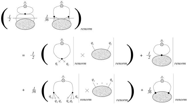
Figure 2: Counterterm renormalization of the last two diagrams in Eq.(3.17). (Cut legs indicate amputations.)

\begin{picture}(10.0,7.0)\end{picture}

So the only UV divergence in Eq.(3.17) which cannot be cured by existing counterterms is that coming from the first (i.e. free field or ring) diagram. The foregoing divergence is evidently temperature independent (to see that, simply use an explicit form of the free thermal propagator $\hbox{\upright\hbox to0.0pt{I\hss}\kern 1.7ptD}_{11}$). Hence, if we define

$$\langle\phi^{2}\rangle_{\mbox{\footnotesize{renorm}}}=\langle[\phi^{2}]\rangle-\langle 0|[\phi^{2}]|0\rangle,$$ (3.19)

or, alternatively

$$\langle\phi^{2}\rangle_{\mbox{\footnotesize{renorm}}}=\langle[\phi^{2}]\rangle-\langle[\phi^{2}]\rangle|_{\mbox{\footnotesize{free fields}}}\,,$$ (3.20)

we get finite quantities, as desired. On the other hand, we should emphasize that

$$\langle\phi^{2}\rangle-\langle 0|\phi^{2}|0\rangle=Z_{\phi^{2}}\left\{\langle[\phi^{2}]\rangle-\langle 0|[\phi^{2}]|0\rangle\right\}\not=\mbox{finite in $D$=4}\,.$$ (3.21)

An extension of the previous reasonings to any $N>1$ is straightforward, only difference is that we must deal with operator mixing which makes (3.19) and (3.20) less trivial.

The important lesson which we have learnt here is that the naive “double dotted” normal product (i.e. subtraction of the vacuum expectation value from a given operator) does not generally give a finite result. The former is perfectly suited for the free theory ($Z_{\Sigma\phi^{2}}=1$) but in the interacting case we must resort to the prescription (3.19) or (3.20) instead.

3.2 Renormalization of the energy–momentum tensor

In order to calculate the hydrostatic pressure, we need to find such $\langle\Theta^{\mu\nu}_{c}\rangle|_{\mbox{\footnotesize{renorm}}}$ which apart from being finite is also consistent with our derivation of the hydrostatic pressure introduced in the introductory Section. In view of the previous treatment, we however cannot, however, expect that $\Theta^{\mu\nu}_{c}$ will be renormalized multiplicatively. Instead, new terms with a different structure than $\Theta^{\mu\nu}_{c}$ itself will be generated during renormalization. The latter must add up to $\Theta^{\mu\nu}_{c}$ in order to render $D^{\mu\nu}(x^{n}|y)$ finite.

Now, the key ingredient exploited in Eq.(2.5) is the conservation law (continuity equation). It is well known that one can “modify” $\Theta^{\mu\nu}_{C}$ in such a way that the new tensor $\Theta^{\mu\nu}$ preserves the convergence properties of $\Theta^{\mu\nu}_{c}$. Such a modification (the Pauli transformation) reads

$$\Theta^{\mu\nu}=\Theta^{\mu\nu}_{c}+\partial_{\lambda}X^{\lambda\mu\nu}\,,$$

$$X^{\lambda\mu\nu}=-X^{\mu\lambda\nu}\,.$$ (3.22)

For scalar fields (3.22) is the only transformation which neither changes the divergence properties of $\Theta^{\mu\nu}_{c}$ nor the generators of the Poincare group constructed out of $\Theta^{\mu\nu}_{c}$ [6, 27, 48, 52]. Because the renormalized (or improved) energy momentum tensor must be conserved (otherwise theory would be anomalous), it has to mix with $\Theta^{\mu\nu}_{c}$ under renormalization only via the Pauli transformation, i.e.

$$[\Theta^{\mu\nu}_{c}]=\Theta^{\mu\nu}_{c}+\partial_{\lambda}X^{\lambda\mu\nu}\,.$$

In order to determine $X^{\lambda\mu\nu}$, we should realize that its role is to cancel divergences present in $\Theta^{\mu\nu}_{c}$. Such a cancellation can be, however, performed only by means of composite operators which are even in the number of fields (note that $\Theta^{\mu\nu}_{c}$ is even in fields and Green’s functions with the odd number of fields vanish). Recalling the condition that renormalization can mix only operators with dimension less or equal, we see that the dimension of $X^{\lambda\mu\nu}$ must be $D-1$, and that $X^{\lambda\mu\nu}$ must be quadratic in fields. The only possible form which is compatible with tensorial structure (3.22) is then

$$X^{\lambda\mu\nu}=\sum_{a,b=1}^{N}c_{ab}(\lambda_{r};D)\;\left(\partial^{\mu}g^{\lambda\nu}-\partial^{\lambda}g^{\mu\nu}\right)\;\phi_{a}\phi_{b}\,.$$ (3.23)

From the fact that $\Theta^{\mu\nu}_{c}$ and $[\Theta^{\mu\nu}_{c}]$ are $O(N)$ invariant (see Eq.(3.2)), $\partial_{\lambda}X^{\lambda\mu\nu}$ must be also $O(N)$ invariant, so $c_{ab}=\delta_{ab}c$. Thus, finally we can write

$$[\Theta^{\mu\nu}_{c}]=\Theta^{\mu\nu}_{c}+c(\lambda_{r};D)\;\sum_{a=1}^{N}\left(\partial^{\mu}\partial^{\nu}-g^{\mu\nu}\partial^{2}\right)\;\phi_{a}^{2}\,,$$ (3.24)

with $c=c_{0}+\sum(\mbox{poles})$, here $c_{0}$ is analytic in $D$. Structure of $c(\lambda_{r};D)$ could be further determined, similarly as in the $N=1$ theory, employing a renormalization group equation [40]. We do not intend to do that as the detailed structure of $c$ will show totally irrelevant for the following discussion, however, it turns out to be important in non–equilibrium cases.

Now, similarly as before, $[\Theta^{\mu\nu}_{c}]$ gives the finite composite Green’s functions if $n>0$ but the expectation value $\langle[\Theta^{\mu\nu}_{c}]\rangle$ is divergent (for discussion of the $N=1$ theory see, e.g., Brown [40]). The unrenormalized DS equation for $D^{\mu\nu}(0|0)$ reads [6]

The structure of the composite vertices in (3.26) is that described at the beginning of this Section. Note that the amputated composite Green’s functions in individual parentheses are of the same order in $\lambda_{r}$. Performing the counterterm renormalization as in the case of $\langle[\phi^{2}]\rangle$, we factorize the graphs inside of parentheses into the product of the renormalized 2– (and 6–) point composite Green’s function and the renormalized full 2– (and 6–) point Green’s function. The latter are finite. The UV divergences arisen during the integrations over momenta connecting both composite and full Green’s functions are precisely cancelled by the remaining counterterm diagrams. Only divergence comes from the free–field contribution, more precisely from the $T=0$ ring diagram. Defining

$$\langle\Theta^{\mu\nu}_{c}\rangle|_{\mbox{\footnotesize{renorm}}}=\langle[\Theta^{\mu\nu}_{c}]\rangle-\langle 0|[\Theta^{\mu\nu}_{c}]|0\rangle,$$ (3.26)

or

$$\langle\Theta^{\mu\nu}_{c}\rangle|_{\mbox{\footnotesize{renorm}}}=\langle[\Theta^{\mu\nu}_{c}]\rangle-\langle[\Theta^{\mu\nu}_{c}]\rangle|_{\mbox{\footnotesize{free field}}}\,,$$ (3.27)

we get the finite expressions. Note that the conservation law is manifest in both cases. In equilibrium (and in $T=0$) we can, due to space–time translational invariance of $\langle\ldots\rangle$, write

$$\langle[\Theta^{\mu\nu}_{c}]\rangle=\langle\Theta^{\mu\nu}_{c}\rangle+\partial_{\lambda}\langle X^{\lambda\mu\nu}\rangle=\langle\Theta^{\mu\nu}_{c}\rangle\,.$$ (3.28)

Using (3.26) or (3.27) we get either the thermal interaction pressure or the interaction pressure, respectively. This can be explicitly written as

$${\cal P}_{\mbox{\footnotesize{th.int.}}}(T)={\cal P}(T)-{\cal P}(0)=-\frac{1}{(D-1)}\sum_{i=1}^{D-1}\left\{\langle\Theta_{c\;i}^{i}\rangle-\langle 0|\Theta_{c\;i}^{i}|0\rangle\right\}\,,$$ (3.29)

or

$${\cal P}_{\mbox{\footnotesize{int.}}}(T)={\cal P}(T)-{\cal P}_{\mbox{\footnotesize{free field}}}(T)=-\frac{1}{(D-1)}\sum_{i=1}^{D-1}\left\{\langle\Theta_{c\;i}^{i}\rangle-\langle\Theta_{c\;i}^{i}\rangle|_{\mbox{\footnotesize{free field}}}\right\}.$$ (3.30)

In order to keep connection with calculations done by Drummond et al. in [2] we shall in the sequel deal with the thermal interaction pressure only. If instead of an equilibrium, a non–equilibrium medium would be in question, translational invariance of $\langle\ldots\rangle$ might be lost, in that case either prescription (3.26) or (3.27) is obligatory, and consequently $c(\lambda_{r};D)$ in (3.24) must be further specified.

4 Hydrostatic pressure - calculation

In the previous section we have prepared ground for a hydrostatic pressure calculations. In this section we aim to apply the previous results to the massive $O(N)\;\phi^{4}$ theory in the large–$N$ limit. Anticipating an out of equilibrium application, we shall use the real–time formalism even if the imaginary–time one is more natural in the equilibrium context. As we aim to evaluate the hydrostatic pressure in 4 dimensions, we use here, similarly as in the previous Section, the usual dimensional regularization to regulate the theory (i.e. here and throughout we keep $D$ slightly away from the physical value $D=4$).

In order to actually pursue the pressure calculation we feel it is necessary to briefly review the mass and coupling renormalization of the model at hand. This will also help to clarify the notation used. While we hope to provide all essentials requisite for our task, good discussion of alternative approaches and renormalization prescriptions may be obtained for instance in [32, 33, 36].

4.1 Mass renormalization

In the Dyson multiplicative renormalization the fact that the complete propagator has a pole at the physical mass leads to the usual mass renormalization prescription [27]:

$$m_{r}^{2}=m_{0}^{2}+\Sigma(m^{2}_{r})\,,$$ (4.1)

where $m_{r}$ is renormalized mass and $\Sigma(m_{r}^{2})$ is the proper self–energy evaluated at the mass shell; $p^{2}=m_{r}^{2}$. In fact, Eq.(4.1) is nothing but the statement that 2–point vertex function $\Gamma^{(2)}_{r}$ evaluated at the mass-shell must vanish. The Dyson–Schwinger equation corresponding to the proper self–energy reads [32, 41, 58, 59]:

where hatched blobs represent 2–point connected Green’s functions whilst cross–hatched blobs represent proper vertices $\Gamma^{(4)}_{r}$ (i.e. 1PI 4–point Green’s function). As $\Sigma^{aa}$ are the same for all $a$, we shall simplify notation and write $\Sigma$ instead. In the sequel the following convention is accepted:

The second term in (4.2) actually does not contribute in the large–$N$ limit. It is easy to see that the third term does not contribute either. This is because each hatched blob behaves at most as $N^{0}$ whilst $\Gamma^{(4)}$ goes maximally as $N^{-1}$. Consequently, various contributions from the first graph in (4.2) contribute at most $N^{0}$, whereas in the second graph the contributions contribute up to order $N^{-1}$. So the first diagram dominates, provided we retain only such 2–point connected Green’s functions which are proportional to $N^{0}$ (as mentioned in the footnote, these are comprised only of tadpole loops.). After neglecting the “setting sun” graph, Eg.(4.2) generates upon iterating the so called superdaisy diagrams [2, 28, 41].

Let us now define $\Sigma(m^{2}_{r})=\lambda_{0}\;{\cal M}(m_{r}^{2})$. Because the tadpole diagram in (4.2) can be easily resumed we observe that

$${\cal M}(m_{r}^{2})=\frac{1}{2}\int\frac{d^{D}q}{(2\pi)^{D}}\;\frac{i}{q^{2}-m_{0}^{2}-\Sigma(m^{2}_{r})+i\epsilon}=\frac{1}{2}\int\frac{d^{D}q}{(2\pi)^{D}}\;\frac{i}{q^{2}-m^{2}_{r}+i\epsilon}\,,$$ (4.3)

hence we see that $\Sigma$ is external–momentum independent. If we had started with the renormalization prescription: $i\Gamma^{(2)}_{r}(p^{2}=0)=-m^{2}_{r}$, we would arrived at (4.1) as well (this is not the case for $N=1$!).

At finite temperature the strategy is analogous. Due to a doubling of degrees of freedom, the full propagator is a $2\times 2$ matrix. The latter satisfies, similarly as at $T=0$, Dyson’s equation

$$\hbox{\upright\hbox to0.0pt{I\hss}\kern 1.7ptD}=\hbox{\upright\hbox to0.0pt{I\hss}\kern 1.7ptD}_{F}+\hbox{\upright\hbox to0.0pt{I\hss}\kern 1.7ptD}_{F}\left(-i{\cal{\bf\Sigma}}\right)\hbox{\upright\hbox to0.0pt{I\hss}\kern 1.7ptD}\,.$$ (4.4)

An important point is that there exists a real, non–singular matrix IM (Bogoliubov matrix) [6, 7, 10] having a property that

$$\hbox{\upright\hbox to0.0pt{I\hss}\kern 1.7ptD}_{F}=\hbox{\upright\hbox to0.0pt{I\hss}\kern 1.7ptM}\left(\begin{array}[]{cc}i\Delta_{F}&0\\ 0&-i\Delta^{*}_{F}\end{array}\right)\hbox{\upright\hbox to0.0pt{I\hss}\kern 1.7ptM}\;\;\;\;\mbox{and}\;\;\;\;{\cal{\bf\Sigma}}=\hbox{\upright\hbox to0.0pt{I\hss}\kern 1.7ptM}^{-1}\left(\begin{array}[]{cc}\Sigma_{T}&0\\ 0&-\Sigma^{*}_{T}\end{array}\right)\hbox{\upright\hbox to0.0pt{I\hss}\kern 1.7ptM}^{-1}\,.$$ (4.5)

Here $\Delta_{F}$ is the standard Feynman propagator and * denotes the complex conjugation. Consequently, the full matrix propagator may be written as

$$\hbox{\upright\hbox to0.0pt{I\hss}\kern 1.7ptD}=\hbox{\upright\hbox to0.0pt{I\hss}\kern 1.7ptM}\left(\begin{array}[]{cc}\frac{i}{p^{2}-m_{0}^{2}-\Sigma_{T}+i\epsilon}&0\\ 0&\frac{-i}{p^{2}-m_{0}^{2}-\Sigma^{*}_{T}-i\epsilon}\end{array}\right)\hbox{\upright\hbox to0.0pt{I\hss}\kern 1.7ptM}\,.$$ (4.6)

Similarly as in many body systems, the position of the (real) pole of ID in $p^{2}$ fixes the temperature–dependent effective mass $m_{r}(T)$ [7, 60]. The latter is determined by the equation

$$m_{r}^{2}(T)=m_{0}^{2}+\mbox{Re}\left(\Sigma_{T}(m^{2}_{r}(T))\right)\,.$$ (4.7)

From the explicit form of IM it is possible to show [6, 7] that $\mbox{Re}{\cal{\bf\Sigma}}_{11}=\mbox{Re}\Sigma_{T}$. As before, the structure of the proper self–energy can be deduced from the corresponding Dyson–Schwinger equation. Following the usual real–time formalism convention (type–1 vertex $\sim-i\lambda_{0}$, type–2 vertex $\sim i\lambda_{0}$ ), the former reads:

and similarly for $\hbox{\upright\hbox to0.0pt{I\hss}\kern 1.7ptD}_{22}$. In (4.8) we have omitted diagrams which are of order ${\cal O}(1/N)$ or less. Note that the fact that no setting sun diagrams are present implies that the off–diagonal elements of ${\cal{\bf\Sigma}}$ are zero. Inspection of Eq.(4.8) reveals that

$${\cal{\bf\Sigma}}_{11}=\frac{\lambda_{0}}{2}\;\int\frac{d^{D}q}{(2\pi)^{D}}\;{\hbox{\upright\hbox to0.0pt{I\hss}\kern 1.7ptD}}_{11}(q;T)\;\;\;\mbox{and}\;\;\;{\cal{\bf\Sigma}}_{22}=-\frac{\lambda_{0}}{2}\;\int\frac{d^{D}q}{(2\pi)^{D}}\;{\hbox{\upright\hbox to0.0pt{I\hss}\kern 1.7ptD}}_{22}(q;T)\,.$$ (4.9)

It directly follows from Eq.(4.9) that both ${\cal{\bf\Sigma}}_{11}$ and ${\cal{\bf\Sigma}}_{22}$ are external–momentum independent and real . If we define $\Sigma_{T}(m_{r}^{2}(T))=\lambda_{0}\;{\cal M}_{T}(m_{r}^{2}(T))$, then Eq.(4.7) through Eq.(4.9) implies that

$$m_{r}^{2}(T)=m^{2}_{0}+\lambda_{0}\;{\cal M}_{T}(m_{r}^{2}(T))\,.$$ (4.10)

A resumed version of $\hbox{\upright\hbox to0.0pt{I\hss}\kern 1.7ptD}_{11}$ is easily obtainable from (4.6) [6, 7] and consequently (4.9) yields

$${\cal M}_{T}(m_{r}^{2}(T)) = \frac{1}{2}\;\int\frac{d^{D}q}{(2\pi)^{D}}\;\left\{\frac{i}{q^{2}-m^{2}_{r}(T)+i\epsilon}\;\;+\;(4\pi)\;\delta^{+}(q^{2}-m^{2}_{r}(T))\;\frac{1}{e^{q_{0}\beta}-1}\right\}$$ (4.11)

$$= -\int\frac{d^{D}q}{(2\pi)^{D}}\;\frac{\varepsilon(q_{0})}{e^{q_{0}\beta}-1}\;\mbox{Im}\frac{1}{q^{2}-m_{r}^{2}(T)+i\epsilon}.$$

Let us remark that (4.11) is manifestly independent of any particular real–time formalism version.

In passing it may be mentioned that because ${\cal{\bf\Sigma}}_{11}(m^{2}_{r})$ is momentum independent, the wave function renormalization $Z_{\phi}=1$. (The Källen–Lehmann representation requires the renormalized propagator to have a pole of residue $i$ at $p^{2}=m^{2}_{r}$. The former in turn implies that $Z_{\phi}=(1-{\cal{\bf\Sigma}}_{11}^{\prime}(p^{2})|_{p^{2}=m^{2}_{r}})^{-1}=1$.) Trivial consequence of the foregoing fact is that $\Gamma^{(2)}_{r}=\Gamma^{(2)}$ and $\Gamma^{(4)}_{r}=\Gamma^{(4)}$.

4.2 Coupling constant renormalization

Let us choose the coupling constant to be defined at $T=0$. This will have the advantage that the high temperature expansion of the pressure (see Section 5) will become more transparent. In addition, such a choice will allow us to select safely the part of the parameter space in which spontaneous symmetry breakdown is not possible. An alternative renormalization procedure based on the affective action is presented in [32].

By assumption the fields $\phi_{a}$ have non–vanishing masses, so we can safely choose the renormalization prescription for $\lambda_{r}$ at $s=0$ ($s$ is the standard Mandelstam variable). For example, one may require that for the scattering $aa\rightarrow bb$

$$\Gamma^{(4)}(s=0)=-\lambda_{r}/N,\;\;\;\;\;(b\not=a)\,.$$ (4.12)

The formula (4.12) clearly agrees with the tree level value $\Gamma_{tree}^{(4)\;aabb}(s=0)=-\lambda_{0}/N$. Let us also mention that Ward’s identities corresponding to the internal $O(N)$ symmetry enforce $\Gamma^{(4)\;aaaa}$ to obey the constraint

$$\Gamma^{(4)\;aaaa}(p_{1};p_{2};p_{3};p_{4}) = \Gamma^{(4)\;bbaa}(p_{1};p_{2};p_{3};p_{4})+\Gamma^{(4)\;baba}(p_{1};p_{2};p_{3};p_{4})$$ (4.13)

$$+ \Gamma^{(4)\;baab}(p_{1};p_{2};p_{3};p_{4})\,,$$

for any $b\not=a$. The structure of $\Gamma^{(4)}$ is encoded in the Dyson–Schwinger equation (4.14) (see also  [27, 58]).

In the latter the sum $\sum_{i=1}^{3}$ schematically represents a summation over $s$, $t$ and $u$ scattering channels. For clarity’s sake the internal indices are suppresses. Similarly as before, we can argue that both the third and fourth graphs contribute at most $N^{-2}$, whilst the second (“fish”) graph may contribute up to order $N^{-1}$. So in the large–$N$ limit the last three diagrams may be neglected, provided we keep in the $4$–point vertex function only graphs proportional to $N^{-1}$. However, the former can be only fulfilled if we retain such a “fish” graph where summation over internal index on the loop is allowed. Remaining two graphs in the sum $\sum_{i=1}^{3}$ (i.e., $t$ and $u$ scattering channels) are suppressed by the factor $N^{-1}$ as the internal index on the loop is fixed. In this way we are left with the relation

$$\Gamma^{(4)\;aabb}(s=0)$$

$$\mbox{}=-\frac{\lambda_{0}}{N}-\left.\frac{i\lambda_{0}}{2N}\sum_{c\not=b}\int\frac{d^{D}q}{(2\pi)^{D}}\;\Gamma^{(4)\;bbcc}(s)\;\frac{i}{\left(q^{2}-m_{r}^{2}+i\epsilon\right)}\;\frac{i}{\left((q-Q)^{2}-m_{r}^{2}+i\epsilon\right)}\right|_{s=0}$$

$$\mbox{}=-\frac{\lambda_{0}}{N}-\frac{\lambda_{0}\lambda_{r}(N-1)}{2N^{2}}\int^{1}_{0}dx\int\frac{d^{D}q}{(2\pi)^{D}}\;\left.\frac{i}{\left(q^{2}-m_{r}^{2}+x(1-x)s+i\epsilon\right)^{2}}\right|_{s=0}\,,$$

(4.15)

with $Q=p_{1}+p_{2}$ and $s=Q^{2}$, $p_{1},p_{2}$ are the external momenta. To leading order in $1/N$ we may equivalently write

$$\lambda_{r}=\lambda_{0}+\lambda_{0}\lambda_{r}\;{\cal M}^{\prime}(m^{2}_{r})\,,$$ (4.16)

the prime means differentiation with respect to $m_{r}^{2}$; ${\cal M}(m^{2}_{r})$ is defined by (4.3). Evaluating explicitly ${\cal M}^{\prime}(m^{2}_{r})$, we get from (4.16)

$$\lambda_{0}=\frac{\lambda_{r}}{1-\lambda_{r}\Gamma(2-\frac{D}{2})\;(m_{r})^{D-4}/2\;(4\pi)^{\frac{D}{2}}}\,.$$ (4.17)

Assuming that both $\lambda_{0}\geq 0$ and $\lambda_{r}\geq 0$ (note $\lambda_{r}<0$ would be incompatible with $\lambda_{0}\geq 0$ and $m_{r}^{2}>0$), we can infer from (4.17) that

$$0\leq\lambda_{r}\leq\frac{2(4\pi)^{\frac{D}{2}}(m_{r})^{4-D}}{\Gamma(2-\frac{D}{2})}\,,$$ (4.18)

and so for $D=4$ we inevitably get that $\lambda_{r}=0$. The latter indicates that the theory is trivial [2, 26, 34], or, in other words, the $O(N)\;\phi^{4}$ theory is a renormalized free theory in the large–$N$ limit. This conclusion is also consistent with the observation that the theory does not posses any non–trivial UV fixed point in the large–$N$ limit [26, 34, 35, 61].

On the other hand, if we were assuming that $\lambda_{0}<0$, we would get indeed a non–trivial renormalized field theory in $D=4$ (actually, from (4.17) we see that $\lambda_{0}\rightarrow 0_{-}$ , provided that $\lambda_{r}$ is fixed and positive and $D\rightarrow 4_{-}$). However, as it was pointed out in refs. [2, 26, 34, 36], such a theory is intrinsically unstable as the ground–state energy is unbounded from below. This is reflected, for instance, in the existence of tachyons in the theory [2, 34, 36, 62], therefore the case with negative $\lambda_{0}$ is clearly inconsistent.

The straightforward remedy for this situation was suggested by Bardeen and Moshe [34]. They showed that the only meaningful (stable) $O(N)\;\phi^{4}$ theory in the large–$N$ limit is that with $\lambda_{r},\lambda_{0}\geq 0$. This is provided that we view it as an effective field theory at momenta scale small compared to a fixed UV cut–off $\Lambda$. The cut–off itself is further determined by (4.16) because in that case (assuming $m_{r}\ll\Lambda$)

$$\lambda_{0}=\frac{\lambda_{r}}{1-\frac{\lambda_{r}}{32\pi^{2}}\mbox{ln}(\frac{\Lambda^{2}}{m^{2}_{r}})}\,,$$ (4.19)

which implies that for $\lambda_{r},\lambda_{0}\geq 0$ we have $\Lambda^{2}<m^{2}_{r}\;\mbox{exp}(\frac{32\pi^{2}}{\lambda_{r}})$. The case $\Lambda^{2}=m^{2}_{r}\;\mbox{exp}(\frac{32\pi^{2}}{\lambda_{r}})$ corresponds to the Landau ghost [63] (tachyon pole [2, 34]). For reasonably small $\lambda_{r}$, $\Lambda$ is truly huge and so it does not represent any significant restriction.

In passing we may observe that from (4.1) and (4.19)

$$\frac{m_{r}^{2}}{\lambda_{r}}=\frac{m_{0}^{2}}{\lambda_{0}}+\frac{1}{23\pi^{2}}\ \Lambda^{2}\,,$$ (4.20)

and so the fraction $m_{r}^{2}/\lambda_{r}$ is renormalization invariant. It was argued in [34] that for the part of the parameter space where $\lambda_{0}>0$ and $m_{r}^{2}/\lambda_{r}>0$ the ground state is $O(N)$ symmetric, Goldstone phenomena cannot materialize and hence the expectation value of the field is zero. The latter fact has been implicitly used, for instance, in the derivation our Dyson–Schwinger equations. To avoid a delicate discussion of the phase structure of the $O(N)\ \phi^{4}$ theory and to emphasize our primary objective - i.e. hydrostatic pressure calculation, we confine ourselves to the parameter space defined above. Such an effective theory will provide a suitable playground to explore all the basic salient points involved in the hydrostatic pressure calculation. Furthermore, because the mass–shift equation (gap equation) has a particularly simple form in this case the hight–$T$ analysis of the hydrostatic pressure will be easy to perform.

4.3 Resumed hydrostatic pressure

The partition function $Z$ has a well known path-integral representation at finite temperature, namely

$$Z[T]=\mbox{exp}(\Phi[T])=\int{\cal D}\phi\;\mbox{exp}(iS[\phi;T])\,,$$

$$S[\phi;T]=\int_{C}d^{D}x\;{\cal L}(x)\,.$$ (4.21)

Here $\Phi=-\beta\Omega$ is a Massieu function (the Legendre transform of the entropy) [6, 42, 43, 44] and $\int_{C}d^{D}x=\int_{C}dx_{0}\int_{V}d^{D-1}{\cal{\bf x}}$ with the subscript $C$ suggesting that the time runs along some contour in the complex plane. In the real–time formalism, which we adopt throughout, the most natural version is the so called Keldysh–Schwinger one [6, 7], which is represented by the contour in Fig.3.

Figure 3: The Keldysh–Schwinger time path.

Let us mention that the fields within the path–integral (4.21) are further restricted by the periodic boundary condition (KMS condition) [6, 7, 10] which in our case reads:

$$\phi_{a}(t_{i}-i\beta,{\cal{\bf x}})=\phi_{a}(t_{i},{\cal{\bf x}})\,.$$

As explained in Section 3, we can use for a pressure calculation the canonical energy–momentum tensor $\Theta^{\mu\nu}_{c}$. Employing for $\Theta^{\mu\nu}_{c}(x)$ its explicit form (3.2) together with (3.6), one may write

$$\langle\Theta^{\mu\nu}_{c}\rangle=\frac{N}{2}\;\int\frac{d^{D}q}{(2\pi)^{D}}(2q^{\mu}q^{\nu}-g^{\mu\nu}(q^{2}-m^{2}_{0}))\;\hbox{\upright\hbox to0.0pt{I\hss}\kern 1.7ptD}_{11}(q;T)\;\;+\frac{\lambda_{0}}{8N}g^{\mu\nu}\left\langle\left(\sum_{a=1}^{N}\phi_{a}^{2}(0)\right)^{2}\right\rangle\,,$$ (4.22)

where $\hbox{\upright\hbox to0.0pt{I\hss}\kern 1.7ptD}_{11}$ is the Dyson–resumed thermal propagator [6, 7], i.e.

$$\hbox{\upright\hbox to0.0pt{I\hss}\kern 1.7ptD}_{11}(q;T)=\frac{i}{q^{2}-m^{2}_{r}(T)+i\epsilon}\;\;+(2\pi)\;\delta(q^{2}-m^{2}_{r}(T))\;\frac{1}{e^{|q_{0}|\beta}-1}\,.$$ (4.23)

Note that we have exploited in (4.22) the fact that the expectation value of $\Theta^{\mu\nu}_{c}(x)$ is $x$ independent. On the other hand, in (4.23) we have used the fact that $m^{2}_{r}$ is $q$ independent. In order to calculate the expectation value of the quartic term in Eq.(4.22), let us observe (c.f. (4.21)) that the derivative of $\Phi$ with respect to the bare coupling $\lambda_{0}$ (taken at fixed $m_{0}$) gives

$$\frac{\partial\Phi[T]}{\partial\lambda_{0}}=-\frac{i}{8\;N}\;\int_{C}d^{D}x\left\langle\left(\sum_{a=1}^{N}\phi_{a}^{2}(0)\right)^{2}\right\rangle\,,$$

which implies that

$$\left\langle\left(\sum_{a=1}^{N}\phi_{a}^{2}(0)\right)^{2}\right\rangle=-\frac{N8}{\beta V}\;\frac{\partial\Phi[T]}{\partial\lambda_{0}}\,.$$ (4.24)

The key point now is that we can calculate $\Phi[T]$ in a non–perturbative form. (The latter is based on the fact that we know the Dyson–resumed propagator $\hbox{\upright\hbox to0.0pt{I\hss}\kern 1.7ptD}_{11}(q;T)$ (see (4.23).) Indeed, taking derivative of $\Phi$ with respect to $m_{0}^{2}$ (keeping $\lambda_{0}$ fixed) we obtain

$$\frac{\partial\Phi[T]}{\partial m_{0}^{2}} = -\frac{iN}{2}\int_{C}d^{D}x\left\langle\phi^{2}(0)\right\rangle=-\frac{\beta VN}{2}\int\frac{d^{D}q}{(2\pi)^{D}}\;\hbox{\upright\hbox to0.0pt{I\hss}\kern 1.7ptD}_{11}(q;T)$$ (4.25)

$$= -\beta VN\;{\cal M}_{T}(m_{r}^{2}(T))\,,$$

thus

$$\Phi[T;\lambda_{0};m_{0}^{2}]=\beta VN\;\int_{m_{0}^{2}}^{\infty}d{\hat{m}}_{0}^{2}\;{\cal M}_{T}({\hat{m}}_{r}^{2}(T))\;\;+\Phi[T;\lambda_{0};\infty]\,.$$ (4.26)

Let us note that $\Phi[T;\lambda_{0};\infty]$ is actually zero because $\Phi[T;\lambda_{0};m^{2}_{0}]$ has the standard loop expansion [6, 58] depicted in Fig.4.

Figure 4: First few bubble diagrams in the $\Phi$ expansion.

It is worth mentioning that in the latter expansion one must always have at least one type–1 vertex [6]. The RHS of Fig.4 clearly tends to zero for $m_{0}\rightarrow\infty$ as all the (free) thermal propagators from which the individual diagrams are constructed tend to zero in this limit. The former result can be also deduced from the CJT effective action formalism [28] or from a heuristic argumentation based on a thermodynamic pressure [2]. Note that in the large–$N$ limit the fourth and fifth diagrams in Fig.4 must be omitted.

The expectation value (4.24) can be now explicitly written as

$$\left\langle\left(\sum_{a=1}^{N}\phi_{a}^{2}(0)\right)^{2}\right\rangle=8N^{2}\;\int_{m_{0}^{2}}^{\infty}d{\hat{m}}_{0}^{2}\;\int\frac{d^{D}q}{(2\pi)^{D}}\;\frac{\varepsilon(q_{0})}{e^{q_{0}\beta}-1}\;\mbox{Im}\left(\frac{\frac{\partial\Sigma_{T}({\hat{m}}_{r}^{2}(T))}{\partial\lambda_{0}}}{(q^{2}-{\hat{m}}^{2}_{r}+i\epsilon)^{2}}\right)\,.$$ (4.27)

In fact, the differentiation of the proper self–energy in (4.27) can be carried out easily. Using (4.10), we get

$$\frac{\partial\Sigma_{T}}{\partial\lambda_{0}}=\frac{\Sigma_{T}}{\lambda_{0}}+\lambda_{0}{\cal M}_{T}^{\prime}\;\frac{\partial\Sigma_{T}}{\partial\lambda_{0}}\;\;\Rightarrow\;\;\frac{\partial\Sigma_{T}}{\partial\lambda_{0}}=\frac{\Sigma_{T}}{\lambda_{0}(1-\lambda_{0}{\cal M}^{\prime}_{T})}\,.$$

From Eq.(4.10) it directly follows that

$$\frac{dm_{r}^{2}(T)}{dm_{0}^{2}}=\frac{1}{(1-\lambda_{0}\;{\cal M}^{\prime}_{T})}\,,$$

which, together with the definition of ${\cal M}_{T}$, gives

$$\left\langle\left(\sum_{a=1}^{N}\phi_{a}^{2}(0)\right)^{2}\right\rangle = 8N^{2}\;\int_{m_{r}^{2}(T)}^{\infty}d{\hat{m}}_{r}^{2}\;\int\frac{d^{D}q}{(2\pi)^{D}}\;\frac{\varepsilon(q_{0})}{e^{q_{0}\beta}-1}\;\mbox{Im}\frac{{\cal M}_{T}({\hat{m}}_{r}^{2})}{(q^{2}-{\hat{m}}_{r}^{2}+i\epsilon)^{2}}$$ (4.28)

$$= -\;8N^{2}\;\int_{m_{r}^{2}(T)}^{\infty}d{\hat{m}}_{r}^{2}\;{\cal M}_{T}({\hat{m}}_{r}^{2})\;\frac{\partial{\cal M}_{T}({\hat{m}}_{r}^{2})}{\partial{\hat{m}}_{r}^{2}}$$

$$= 4N^{2}\;{\cal M}_{T}^{2}(m_{r}^{2}(T))\,,$$

where we have exploited in the last line the fact that ${\cal M}_{T}^{2}(m_{r}^{2}\rightarrow\infty)=0$. Let us mention that the crucial point in the previous manipulations was that $m_{r}$ is both real and momentum independent. Collecting our results together, we can write for the hydrostatic pressure per particle (cf. Eq(3.29))

$${\cal P}(T)-{\cal P}(0) = -\;\frac{1}{(D-1)N}\;\left(\langle\Theta^{i}_{c\;i}\rangle-\langle 0|\Theta^{i}_{c\;i}|0\rangle\right)$$ (4.29)

$$= +\;\frac{1}{2}\;\int\frac{d^{D}q}{(2\pi)^{D-1}}\;\left(\frac{2{\cal{\bf q}}^{2}}{(D-1)}\right)\;\frac{\varepsilon(q_{0})}{e^{q_{0}\beta}-1}\;\delta(q^{2}-m_{r}^{2}(T))$$

$$-\;\frac{1}{2}\;\int\frac{d^{D}q}{(2\pi)^{D-1}}\;\left(\frac{2{\cal{\bf q}}^{2}}{(D-1)}\right)\;\delta^{+}(q^{2}-m_{r}^{2}(0))$$

$$+\frac{1}{2\lambda_{0}}\left(\Sigma^{2}_{T}(m_{r}^{2}(T))-\Sigma^{2}(m_{r}^{2}(0))\right)\,.$$

Applying Green’s theorem to the last two integrals and eliminating the surface terms (for details see Appendix A) we find

$${\cal P}(T)-{\cal P}(0) = \frac{1}{2}\;\int\frac{d^{D}q}{(2\pi)^{D-1}}\;\frac{\varepsilon(q_{0})}{e^{q_{0}\beta}-1}\;\theta(q^{2}-m^{2}_{r}(T))$$ (4.30)

$$-\frac{1}{2}\;\int\frac{d^{D}q}{(2\pi)^{D-1}}\;\theta(q_{0})\;\theta(q^{2}-m^{2}_{r}(0))$$

$$+\frac{1}{2\lambda_{0}}\left(\Sigma^{2}_{T}(m_{r}^{2}(T))-\Sigma^{2}(m_{r}^{2}(0))\right)$$

$$\mbox{}=\ {\cal N}_{T}(m_{r}^{2}(T))-{\cal N}(m_{r}^{2}(0))+\frac{1}{2\lambda_{0}}\left(\Sigma^{2}_{T}(m_{r}^{2}(T))-\Sigma^{2}(m_{r}^{2}(0))\right)\,,$$

where we have introduced new functions ${\cal N}_{T}(m^{2}_{r}(T)$ and ${\cal N}(m^{2}_{r})$;

$${\cal N}_{T}(m^{2}_{r}(T)) = \frac{1}{2}\;\int\frac{d^{D}q}{(2\pi)^{D-1}}\;\frac{\varepsilon(q_{0})}{e^{q_{0}\beta}-1}\;\theta(q^{2}-m^{2}_{r}(T))$$

$${\cal N}(m^{2}_{r}) = \lim_{T\rightarrow\;0}{\cal N}_{T}(m^{2}_{r}(T))\,.$$ (4.31)

Eq.(4.30) can be rephrased into a form which exhibits an explicit independence of bar quantities. Using the trivial identity:

$$\frac{1}{2\lambda_{0}}\;\left(\Sigma^{2}_{T}(m_{r}^{2}(T))-\Sigma^{2}(m_{r}(0))\right)$$

$$\mbox{\hskip 42.67912pt}=\frac{1}{2\lambda_{0}}\;\left(\Sigma_{T}(m_{r}^{2}(T))-\Sigma(m^{2}_{r}(0))\right)\left(\Sigma_{T}(m_{r}^{2}(T))+\Sigma(m^{2}_{r}(0))\right)$$

$$\mbox{\hskip 42.67912pt}=\frac{\delta m^{2}(T)}{2}\;\left({\cal M}_{T}(m_{r}^{2}(T))+{\cal M}(m^{2}_{r}(0))\right)\,,$$ (4.32)

we get

$$\mbox{}{\cal P}(T)-{\cal P}(0)$$

$$\mbox{}=\ {\cal N}_{T}(m_{r}^{2}(T))-{\cal N}(m_{r}^{2}(0))+\frac{\delta m^{2}(T)}{2}\;\left({\cal M}_{T}(m_{r}^{2}(T))+{\cal M}(m^{2}_{r}(0))\right)\,,$$ (4.33)

where $\delta m^{2}(T)=m_{r}^{2}(T)-m_{r}^{2}(0)$. Let us finally mention that the finding (4.29) is an original result of this paper. The result (4.33) has been previously obtained by authors [2] in the purely thermodynamic pressure framework.

5 High–temperature expansion of the hydrostatic pressure in $D=4$

In order to obtain the high–temperature expansion of the pressure in $D=4$, it is presumably the easiest to go back to equation (4.29) and employ identity (4.32). Let us split this task into two parts. We firstly evaluate the integrals with potentially UV divergent parts using the dimensional regularization. The remaining integrals, with the Bose–Einstein distribution insertion, are safe of UV singularities and can be computed by means of the Mellin transform technique.

Inspecting (4.29) and (4.32), we observe that the only UV divergent contributions come from the integrals:

$$+ \frac{1}{(D-1)}\int\frac{d^{D}q}{(2\pi)^{D-1}}\;{\cal{\bf q}}^{2}\;\left(\delta^{+}(q^{2}-m^{2}_{r}(T))-\delta^{+}(q^{2}-m^{2}_{r}(0))\right)$$ (5.1)

$$+ \frac{\delta m^{2}(T)}{4}\int\frac{d^{D}q}{(2\pi)^{D}}\;\left(\frac{i}{q^{2}-m^{2}_{r}(T)+i\epsilon}+\frac{i}{q^{2}-m^{2}_{r}(0)+i\epsilon}\right)\,,$$

which, if integrated over, give

$$\mbox{(\ref{4.1})}= + \frac{\Gamma(\frac{-D}{2})\Gamma(\frac{D}{2}+\frac{1}{2})}{(D-1)\Gamma(\frac{D-1}{2})(4\pi)^{\frac{D}{2}}}\left((m^{2}_{r}(T))^{\frac{D}{2}}-(m^{2}_{r}(0))^{\frac{D}{2}}\right)$$ (5.2)

$$+ \frac{\delta m^{2}(T)\;\Gamma(1-\frac{D}{2})}{4(4\pi)^{\frac{D}{2}}}\left((m^{2}_{r}(T))^{\frac{D}{2}-1}+(m^{2}_{r}(0))^{\frac{D}{2}-1}\right)\,.$$

Taking the limit $D=4-2\varepsilon\rightarrow 4$ and using expansions

$$\Gamma(-n+\varepsilon) = \frac{(-1)^{n}}{n!}\left(\frac{1}{\varepsilon}+\sum_{k=1}^{n}\frac{1}{k}-\gamma+{\cal O}(\varepsilon)\right)\,,$$

$$a^{x+\varepsilon} = a^{x}\left(1+\varepsilon\;\mbox{ln}a+{\cal O}(\varepsilon^{2})\right)\,,$$

($\gamma$ is the Euler–Mascheroni constant) we are finally left with

$$\left.\mbox{(\ref{4.1})}\right|_{D\rightarrow 4}=-\frac{m^{2}_{r}(0)m^{2}_{r}(T)}{64\;\pi^{2}}\;\mbox{ln}\left(\frac{m^{2}_{r}(T)}{m^{2}_{r}(0)}\right)+\delta m^{2}(T)\;(m_{r}^{2}(T)+m^{2}_{r}(0))\;\frac{1}{128\;\pi^{2}}\,.$$ (5.3)

The fact that we get finite result should not be surprising as entire analysis of Section 3 was made to show that ${\cal P}(T)-{\cal P}(0)$ defined via $\Theta^{\mu\nu}_{c}$ is finite in $D=4$.

We may now concentrate on the remaining terms in (4.29), the latter read (we might, and we shall, from now on work in $D=4$)

$$\frac{1}{3}\int\frac{d^{4}q}{(2\pi)^{3}}\;{\cal{\bf q}}^{2}\;\frac{1}{e^{|q_{0}|\beta}-1}\;\delta(q^{2}-m_{r}^{2}(T))+\frac{\delta m^{2}(T)}{4}\int\frac{d^{4}q}{(2\pi)^{3}}\;\frac{1}{e^{|q_{0}|\beta}-1}\delta(q^{2}-m_{r}^{2}(T))\,.$$ (5.4)

Our following strategy is based on the observation that the previous integrals have generic form:

$$I_{2\nu}(m_{r}) = \int\frac{d^{4}q}{(2\pi)^{3}}\;{\cal{\bf q}}^{2\nu}\;\frac{1}{e^{|q_{0}|\beta}-1}\;\delta(q^{2}-m^{2}_{r})\,,$$ (5.5)

$$= \frac{m_{r}^{2+2\nu}}{2\;\pi^{2}}\;\int_{1}^{\infty}dx\;(x^{2}-1)^{\frac{1+2\nu}{2}}\;\frac{1}{e^{xy}-1}\,,$$

with $\nu=0,1$ and $y=m_{r}\beta$. Unfortunately, the integral (5.5) cannot be evaluated exactly, however, its small $y$ (i.e. high–temperature) behavior can be successfully analyzed by means of the Mellin transform technique [6, 41]. Before going further, let us briefly outline the basic steps needed for such a small $y$ expansion.

The Mellin transform $\hat{f}(s)$ is done by the prescription [6, 41, 64, 65, 66, 67]:

$$\hat{f}(s)=\int_{0}^{\infty}dx\;x^{s-1}\;f(x)\,,$$ (5.6)

with $s$ being a complex number. One can easily check that the inverse Mellin transform reads

$$f(x)=\frac{1}{i(2\pi)}\int_{-i\infty+a}^{i\infty+a}ds\;x^{-s}\;\hat{f}(s)\,,$$ (5.7)

where the real constant $a$ is chosen in such a way that $\hat{f}(s)$ is convergent in the neighborhood of a straight line ($-i\infty+a,\;i\infty+a$). So particularly if $f(x)=\frac{1}{e^{xy}-1}$ one can find ( [66]; formula I.3.19) that

$$\hat{f}(s)=\Gamma(s)\zeta(s)y^{-s}\,,\mbox{\hskip 28.45274pt}(\mbox{Re}s>1)\,,$$ (5.8)

where $\zeta$ is the Riemann zeta function ($\zeta(s)=\sum_{n=1}^{\infty}n^{-s}$). Now we insert the Mellin transform of $f(x)=\frac{1}{e^{xy}-1}$ to (5.5) and interchange integrals (this is legitimate only if the integrals are convergent before the interchange). As a result we have

$$\int_{0}^{\infty}dx\;g(x)\ \frac{1}{e^{xy}-1}=\int_{-i\infty+a}^{i\infty+a}\frac{ds}{i(2\pi)}\;\Gamma(s)\zeta(s)y^{-s}\hat{g}(1-s)\,,$$ (5.9)

with $g(x)=\theta(x-1)\;(x^{2}-1)^{\frac{1+2\nu}{2}}$. Using the tabulated result ( [67]; formula 6.2.32) we find

$$\hat{g}(1-s)=\frac{1}{2}B(-\nu-1+\mbox{$\frac{1}{2}s$};\mbox{$\frac{3}{2}$}+\nu)\,,\mbox{\hskip 42.67912pt}(\mbox{Re}s>2+2\nu)\,,$$ (5.10)

with $B(\;;\;)$ being the beta function. Because the integrand on the RHS of (5.9) is analytic for $\mbox{Re}s>2+2\nu$ and the LHS is finite, we must choose such $a$ that the integration is defined. The foregoing is achieved choosing $\mbox{a}>2+2\nu$. Another useful expressions for $\hat{g}(1-s)$ are ( [67]; formula I.2.34 or I.2.37)

$$\hat{g}(1-s) = B(\mbox{$\frac{3}{2}$}+\nu;-2-2\nu+s)\;{~{}}_{2}F_{1}[-\mbox{$\frac{1}{2}$}-\nu;-2-2\nu+s;-\mbox{$\frac{1}{2}$}-\nu+s;-1]$$

$$= 2^{\frac{1}{2}+\nu}\;B(\mbox{$\frac{3}{2}$}+\nu;-2-2\nu+s)\;{~{}}_{2}F_{1}[-\mbox{$\frac{1}{2}$}-\nu;\mbox{$\frac{3}{2}$}+\nu;-\mbox{$\frac{1}{2}$}-\nu+s;\mbox{$\frac{1}{2}$}]\,,$$

where ${~{}}_{2}F_{1}$ is the (Gauss) hypergeometric function [67]. Using identity

$$\Gamma(2x)=\frac{2^{2x-1}}{\sqrt{\pi}}\;\Gamma(x)\Gamma(x+\mbox{$\frac{1}{2}$})\,,$$

we can write

$$\mbox{(\ref{4.7})}=\frac{\Gamma(\mbox{$\frac{3}{2}$}+\nu)}{4\sqrt{\pi}}\;\int_{-i\infty+a}^{i\infty+a}\frac{ds}{i(2\pi)}\Gamma(\mbox{$\frac{1}{2}$}s)\zeta(s)\left(\mbox{$\frac{1}{2}$}y\right)^{-s}\Gamma(-\nu-1+\mbox{$\frac{1}{2}$}s)\,.$$ (5.11)

The integrand of (5.11) has simple poles in $s=-2n\;(n=1,2,\ldots)$, $s=1$, $s=-2n+2\nu+2\;(n=0,1,\ldots,\nu)$ and double pole in $s=0$. An important point in the former pole analysis was the fact that $\zeta(s)$ has simple zeros in $-2m$ ($m>0$) and only one simple pole in $s=1$. The former together with identity

$$\Gamma\left(\frac{x}{2}\right)\;\pi^{-\frac{x}{2}}\;\zeta(x)=\Gamma\left(\frac{1-x}{2}\right)\;\pi^{\frac{x-1}{2}}\;\zeta(1-x)\,,$$

shows that no double pole except for $s=0$ is present in (5.11). Now, we can close the contour to the left as the value of the contour integral around the large arc is zero in the limit of infinite radius (c.f. [66] and [68]; formula 8.328.1). Using successively the Cauchy theorem we obtain

$$\frac{4\sqrt{\pi}\;\mbox{(\ref{4.7})}}{\Gamma(\mbox{$\frac{3}{2}$}+\nu)}$$

$$\mbox{}=\ \sum_{n=0}^{\nu}y^{2n-2\nu-2}\;\frac{\pi^{-2n+2\nu+2}(-n+\nu)!\;(-1)^{n}|B_{-2n+2\nu+2}|}{n!\;(-2n+2\nu+2)!\;2^{4n-4\nu-4}}$$

$$\mbox{}+\ \sum_{n=1}^{\infty}y^{2n}\;\frac{\pi^{-2n}\;(2n)!\;\zeta(1+2n)\;(-1)^{n+\nu+1}}{n!\;(n+1+\nu)!\;2^{4n-1}}$$

$$\mbox{}+\ y^{-1}\;\frac{\pi\;(-1)^{\nu+1}\;(\nu+1)!\;2^{2\nu+3}}{(2\nu+2)!}+\frac{2\;(-1)^{\nu+1}}{(\nu+1)!}\left\{\mbox{ln}\left(\frac{y}{4\pi}\right)+\gamma-\mbox{$\frac{1}{2}$}\sum_{k=1}^{\nu+1}\frac{1}{k}\right\}\,,$$ (5.12)

where $B_{\alpha}$’s are the Bernoulli numbers. Let us mention that for $\zeta(2n+1)$ only numerical values are available.

Inserting (5.12) back to (5.4), we get for ${\cal P}(T)-{\cal P}(0)$

$${\cal P}(T)-{\cal P}(0)=(\mbox{\ref{4.3}})+\frac{1}{3}\;I_{2}(m_{r}(T))+\frac{\delta m^{2}(T)}{4}\;I_{0}(m_{r}(T))$$

$$\mbox{\hskip 14.22636pt}=\frac{T^{4}\;\pi^{2}}{90}-\frac{T^{2}}{24}\left(m^{2}_{r}(T)-\frac{\delta m^{2}(T)}{2}\right)+\frac{T\;m_{r}(T)}{4\;\pi}\left(\frac{m^{2}_{r}(T)}{3}-\frac{\delta m^{2}(T)}{4}\right)$$

$$\mbox{\hskip 14.22636pt}+\;\frac{m_{r}^{2}(T)\;m^{2}_{r}(0)}{32\;\pi^{2}}\;\left(\mbox{ln}\left(\frac{m_{r}(0)}{T\;4\pi}\right)+\gamma-\frac{1}{2}\right)-\frac{m^{4}_{r}(0)}{128\;\pi^{2}}$$

$$\mbox{\hskip 14.22636pt}-\;\sum_{n=1}^{\infty}\left(m^{2}_{r}(T)-\mbox{$\frac{(n+2)}{2}$}\;\delta m^{2}(T)\right)\;\frac{m_{r}^{2n+2}(T)\;\pi^{-2n-2}\;(2n)!\;\zeta(1+2n)\;(-1)^{1+n}}{T^{2n}\;n!\;(n+2)!\;2^{4n+4}}\,.$$

(5.13)

Note that (5.3) cancelled against the same term in $\frac{1}{3}\;I_{2}(m_{r}(T))+\frac{\delta m^{2}(T)}{4}\;I_{0}(m_{r}(T))$. One can see that (5.13) rapidly converges for large $T$, so that only first four terms dominate at sufficiently high temperature. The aforementioned terms come from the poles nearby the straight line $(-i\infty+a,\;i\infty+a)$ (the more dominant contribution the closer pole). It is a typical feature of the Mellin transform technique that integrals of type

$$\int_{0}^{\infty}dx\;g(x)\;\frac{1}{e^{xy}-1}\,,$$

can be expressed as an expansion which rapidly converges for small $y$ (high–temperature expansion) or large $y$ (low–temperature expansion).

Expansion (5.13) is the sought result. To check its consistency we will apply it to two important cases: high $T$ case and $m_{r}(0)=0$ case. Concerning the first case, note that for a sufficiently large $T$ we can use the high–temperature expansion of $\delta m^{2}(T)$ found in Appendix B. Inserting (B.6) to (5.13) we obtain

$$\mbox{}{\cal P}(T)-{\cal P}(0)=\frac{T^{4}\;\pi^{2}}{90}-\frac{T^{2}\;m^{2}_{r}(T)}{24}+\frac{T^{3}\;m_{r}(T)}{12\pi}$$

$$\mbox{}+\ \frac{\lambda_{r}}{8}\left(\frac{T^{4}}{144}-\frac{T^{3}\;m_{r}(T)}{24\pi}+\frac{T^{2}\;m^{2}_{r}(T)}{16\pi^{2}}\right)+{\cal O}\left(m^{4}_{r}(T)\;\mbox{ln}\left(\frac{m_{r}(T)}{T4\pi}\right)\right)\,.$$ (5.14)

Up to a sign, the result (5.14) coincides with that found by Amelino–Camelia and Pi [3] for the effective potential. Actually, they used instead of the $N\rightarrow\infty$ limit the Hartree–Fock approximation which is supposed to give the same $V_{eff}$ as the leading $1/N$ approximation [63].

As for the second case, we may observe that our discussion of the mass renormalization in Section 3.1 can be directly extended to the case when $m_{r}(0)=0$ (this does not apply to our discussion of $\lambda_{r}$!). Latter can be also seen from the fact that (5.13) is continuous in $m_{r}(0)=0$ (however not analytic). The foregoing implies that the original massless scalar particles acquire the thermal mass $m_{r}^{2}(T)=\delta m^{2}(T)$ . From (5.13) one then may immediately deduce the pressure for massless fields $\phi_{a}$ in terms of $\delta m(T)$. The latter reads

$${\cal P}(T)-{\cal P}(0) = \frac{T^{4}\;\pi^{2}}{90}-\frac{T^{2}\;(\delta m(T))^{2}}{48}+\frac{T\;(\delta m(T))^{3}}{48\;\pi}$$ (5.15)

$$+ \;\sum_{n=1}^{\infty}\frac{(\delta m(T))^{2n+4}\;\pi^{-2n-2}\;(2n)!\;\zeta(1+2n)\;(-1)^{n+1}}{T^{2n}\;(n-1)!\;(n+2)!\;2^{4n+5}}\,.$$

This result is identical to that found by Drummond et al. in [2].

A noteworthy observation is that when the energy of a thermal motion is much higher then the mass of particles in the rest, then the massive theory approaches the massless one. This is justified in the first (high–temperature dominant) term of (5.13) and (5.15). This term is nothing but a half of the black body radiation pressure for photons [42, 43] (photons have two degrees of freedom connected with two transverse polarizations). One could also obtain the temperature dominant contributions directly from the Stefan–Boltzmann law [6, 42, 43] for the density energy (i.e. $\langle\Theta^{00}\rangle$). The formal argument leading to this statement is based on the noticing that at high energy (temperature) the scalar field theory is approximately conformally invariant, which in turn implies that the energy–momentum tensor is traceless [53]. Taking into account the definition of the hydrostatic pressure (2.8), we can with a little effort recover the leading high–temperature contributions for the massive case.

6 Conclusions

In the present article we have clarified the status of hydrostatic pressure in (equilibrium) thermal QFT. The former is explained in terms of the thermal expectation value of the “weighted” space–like trace of the energy–momentum tensor $\Theta^{\mu\nu}$. In classical field theory there is a clear microscopic picture of the hydrostatic pressure which is further enhanced by a mathematical connection (through the virial theorem) with the thermodynamic pressure. In addition, it is the hydrostatic pressure which can be naturally extended to a non–equilibrium medium. Quantum theoretic treatment of the hydrostatic pressure is however pretty delicate. In order to get a sensible, finite answer we must give up the idea of total hydrostatic pressure. Instead, thermal interaction pressure or/and interaction pressure must be used (see (3.29) and (3.30)). We have established this result for a special case when the theory in question is the scalar $\phi^{4}$ theory with $O(N)$ internal symmetry; but it can be easily extended to more complex situations. Moreover, due to a lucky interplay between the conservation of $\Theta^{\mu\nu}$ and the space–time translational invariance of an equilibrium (and $T=0$) expectation value we can use the simple canonical (i.e. unrenormalized) energy–momentum tensor. In the course of our treatment in Section 3 we heavily relied on the counterterm renormalization, which seems to be the most natural when one discusses renormalization of composite Green’s functions. To be specific, we have resorted to the minimal subtraction scheme which has proved useful in several technical points.

We have applied the prescriptions obtained for the QFT hydrostatic pressure to $\phi^{4}$ theory in the–large $N$ limit. The former has the undeniable advantage of being exactly soluble. This is because of the fact that the large–$N$ limit eliminates “nasty” classes of diagrams in the thermal Dyson–Schwinger expansion. The survived class of diagrams (superdaisy diagrams) can be exactly resumed, because the (thermal) proper self–energy ${\cal{\bf\Sigma}}$, as well as the renormalized coupling constant $\lambda_{r}$ are momentum independent. We have also stressed that the $O(N)\;\phi^{4}$ theory in the large–$N$ limit is consistent only if we view it as an effective field theory. Fortunately, the upper bound on the UV cut–off is truly huge, and it does not represent any significant restriction. For the model at hand the resumed form of the pressure with $m_{r}(0)=0$ was firstly derived (in the purely thermodynamic pressure context) by Drummond et al. in [2]. We have checked, using the prescription (3.29) for the thermal interaction pressure, that their results are in agreement with ours. The former is a nice vindication of the validity of the virial theorem for the QFT system at hand. In this connection we should perhaps mention that the latter is by no means obvious. For example, for quantized gauge fields the conformal (trace) anomaly may even invalidate the virial theorem [6]. The fact that this point is indeed non–trivial is illustrated on the QCD case in [69].

The expression for the pressure obtained was in a suitable form which allowed us to take advantage of the Mellin transform technique. We were then able to write down the high–temperature expansion for the pressure in $D=4$ (both for massive and massless fields) in terms of renormalized masses $m_{r}(T)$ and $m_{r}(0)$. We have explicitly checked that all UV divergences present in the individual thermal diagrams “miraculously” cancel in accordance with our analysis of the composite operators in Section 3.

Appendix A Appendix

In this Appendix we give some details of the derivation of Eq.(4.30). We particularly show that the surface integrals arisen during the transition from (4.29) to (4.30) mutually cancel among themselves. As usual, the integrals will be evaluated for integer values of $D$ and corresponding results then analytically continued to a desired (generally complex) $D$.

The key quantity in question is

$$+ \frac{1}{2}\;\int\frac{d^{D}q}{(2\pi)^{D-1}}\left(\frac{2{\cal{\bf q}}^{2}}{(D-1)}\right)\;\frac{\varepsilon(q_{0})}{e^{\beta q_{0}}-1}\;\delta(q^{2}-m^{2}_{r}(T))$$ (A.1)

$$- \frac{1}{2}\;\int\frac{d^{D}q}{(2\pi)^{D-1}}\left(\frac{2{\cal{\bf q}}^{2}}{(D-1)}\right)\;\delta^{+}(q^{2}-m^{2}_{r}(0))\,.$$

Applying Green’s theorem (i.e. integrating by parts with respect to ${\cal{\bf q}}$) on (A.1) one finds

$$\mbox{}\mbox{(\ref{a1})}\ =\ {\cal N}_{T}(m^{2}_{r}(T))-{\cal N}(m^{2}_{r}(0))$$

$$\mbox{}+\ \lim_{R\rightarrow\infty}\;\frac{1}{2(D-1)}\int\frac{dq_{0}}{(2\pi)^{D-1}}\;\int_{\partial S^{D-2}_{R}}d{\cal{\bf s}}\;{\cal{\bf q}}\;\theta(q^{2}-m^{2}_{r}(T))\;\theta(q_{0})\;\left(\frac{2}{e^{\beta q_{0}}-1}+1\right)$$

$$\mbox{}-\ \lim_{R\rightarrow\infty}\;\frac{1}{2(D-1)}\int\frac{dq_{0}}{(2\pi)^{D-1}}\;\int_{\partial S^{D-2}_{R}}d{\cal{\bf s}}\;{\cal{\bf q}}\;\theta(q^{2}-m^{2}_{r}(0))\;\theta(q_{0})\,.$$

As usual, ${\cal{\bf a}}{\cal{\bf b}}=\sum_{i=1}^{D-1}{\cal{\bf a}}_{i}{\cal{\bf b}}_{i}$ and $S^{D-2}_{R}$ is a $(D-2)$–sphere with the radius $R$. The expressions for ${\cal N}_{T}$ and ${\cal N}$ are done by (4.31).

With the relation (LABEL:a2) we can show that the surface terms cancel in the large $R$ limit. Let us first observe that

$$\lim_{R\rightarrow\infty}\;\int\frac{dq_{0}}{(2\pi)^{D-1}}\;\int_{\partial S^{D-2}_{R}}d{\cal{\bf s}}\;{\cal{\bf q}}\;\theta(q^{2}-m^{2}_{r}(T))\;\frac{2\theta(q_{0})}{e^{\beta q_{0}}-1}$$ (A.3)

$$= \lim_{R\rightarrow\infty}\;\frac{2\pi^{\frac{D-1}{2}}R^{D-1}}{\Gamma\left(\frac{D-1}{2}\right)}\;\int\frac{dq_{0}}{(2\pi)^{D-1}}\;\theta(q_{0}^{2}-R^{2}-m^{2}_{r}(T))\;\frac{2\theta(q_{0})}{e^{\beta q_{0}}-1}$$

$$= \lim_{R\rightarrow\infty}\frac{\pi^{\frac{1-D}{2}}R^{D-1}}{2^{D-2}\Gamma\left(\frac{D-1}{2}\right)}\int_{\sqrt{R^{2}+m_{r}^{2}(T)}}^{\infty}dq_{0}\;\frac{2}{e^{\beta q_{0}}-1}\;=\;0\,.$$

In 2–nd line we have exploited Gauss’s theorem and in the last line we have used L’Hôpital’s rule as the expression is in the indeterminate form $0/0$. The remaining surface terms in (LABEL:a2) read

$$\lim_{R\rightarrow\infty}\int\frac{dq_{0}}{(2\pi)^{D-1}}\;\int_{\partial S^{D-2}_{R}}d{\cal{\bf s}}\;{\cal{\bf q}}\;\left\{\theta(q^{2}-m^{2}_{r}(T))-\theta(q^{2}-m^{2}_{r}(0))\right\}\;\theta(q_{0})$$ (A.4)

$$= \lim_{R\rightarrow\infty}\;\frac{\pi^{\frac{1-D}{2}}R^{D-1}}{2^{D-2}\Gamma\left(\frac{D-1}{2}\right)}\;\left\{\int_{\sqrt{R^{2}+m_{r}^{2}(T)}}^{\infty}-\int_{\sqrt{R^{2}+m_{r}^{2}(0)}}^{\infty}\right\}dq_{0}\;=\;0\,.$$

The last identity follows either by applying L’Hôspital’s rule or by a simple transformation of variables which renders both integrals inside of $\{\ldots\}$ equal. Expressions on the last lines in (A.3) and (A.4) can be clearly (single–valuedly) continued to the region $\mbox{Re}D>1$ as they are analytic there. We thus end up with the statement that

$$\mbox{(\ref{a1})}={\cal N}_{T}(m^{2}_{r}(T))-{\cal N}(m^{2}_{r}(0))\,.$$

Appendix B Appendix

In this appendix we shall derive the high–temperature expansion of the mass shift $\delta m^{2}(T)$ in the case when fields $\phi_{a}$ are massive (i.e. $m^{2}_{r}(0)\not=0$).

Consider Eqs.(4.1) and (4.10). If we combine them together, we get easily the following transcendental equation for $\delta m^{2}(T)$

$$\delta m^{2}(T)=\lambda_{0}\left\{{\cal M}(m^{2}_{r}(T))-{\cal M}(m^{2}_{r}(0))+\frac{1}{2}I_{0}(m^{2}_{r}(0)+\delta m^{2}(T))\right\}\,.$$ (B.1)

Here ${\cal M}$ and $I_{0}$ are done by (4.3) and (5.5), respectively.

Now, both $\lambda_{0}$ and ${\cal M}$ are divergent in $D=4$. If we reexpress $\lambda_{0}$ in terms of $\lambda_{r}$, divergences must cancel, as $\delta m^{2}(T)$ is finite in $D=4$. The latter can be easily seen if we Taylor expand ${\cal M}$, i.e.

$${\cal M}(m^{2}_{r}(T))={\cal M}(m^{2}_{r}(0))+\delta m^{2}(T)\;{\cal M}^{\prime}(m^{2}_{r}(0))+\hat{{\cal M}}(m^{2}_{r}(0);\delta m^{2}(T))\,.$$ (B.2)

Obviously, $\hat{{\cal M}}$ is finite in $D=4$ as ${\cal M}$ is quadratically divergent. Inserting (B.2) to (B.1) and employing Eq.(4.16) we get

$$\delta m^{2}(T)=\lambda_{r}\left\{\hat{{\cal M}}(m^{2}_{r}(0);\delta m^{2}(T))+\frac{1}{2}I_{0}(m^{2}_{r}(0)+\delta m^{2}(T))\right\}\,.$$ (B.3)

This is sometimes referred to as the renormalized gap equation. In order to determine $\hat{{\cal M}}$ we must go back to (B.2). From the former we read off that

$$\hat{{\cal M}}(m^{2}_{r}(T);\delta m^{2}(T))$$

$$\mbox{\hskip 22.76228pt}={\cal M}(m^{2}_{r}(T))-{\cal M}(m^{2}_{r}(0))-\delta m^{2}(T)\;{\cal M}^{\prime}(m^{2}_{r}(0))$$

$$\mbox{\hskip 22.76228pt}=\frac{\Gamma(1-\frac{D}{2})}{2(4\pi)^{\frac{D}{2}}}\left\{(m^{2}_{r}(T))^{\frac{D}{2}-1}-(m^{2}_{r}(0))^{\mbox{$\frac{D}{2}$}-1}-\delta m^{2}(T)(\frac{D}{2}-1)\;(m^{2}_{r}(0))^{\frac{D}{2}-2}\right\}$$

$$\mbox{\hskip 22.76228pt}\stackrel{{\scriptstyle D\rightarrow 4}}{{=}}\frac{1}{32\pi^{2}}\left\{m^{2}_{r}(T)\;\mbox{ln}\left(\frac{m^{2}_{r}(T)}{m^{2}_{r}(0)}\right)-\delta m^{2}(T)\right\}\,.$$ (B.4)

So

$$\delta m^{2}(T)=\lambda_{r}\left\{\frac{(m^{2}(0)+\delta m^{2}(T))\;\mbox{ln}\left(1+\frac{\delta m^{2}(T)}{m^{2}_{r}(0)}\right)-\delta m^{2}(T)}{32\pi^{2}}+\frac{1}{2}I_{0}\right\}\,.$$ (B.5)

Analogous relation was also derived in [33] where authors used finite temperature renormalization group. In the latter the zero–momentum renormalization prescription was utilized. Eq.(B.5) was firstly obtained and numerically solved in [2]. It was shown that the solution is double valued. The former behavior was also observed in the effective action approach. Namely by Abbott et al. [36] at $T=0$, and by Bardeen and Moshe [34] at both $T=0$ and $T\not=0$. The relevant solution is only that which fulfils the consistency condition $\delta m^{2}(T)\rightarrow 0$ when $T\rightarrow 0$. For such a solution it can be shown (c.f. [2], Fig.3) that $\frac{\delta m^{2}(T)}{m^{2}_{r}(0)}\ll 1$ for a sufficiently high $T$. So the high–temperature expansion of (B.5) reads

$$\delta m^{2}(T) = \lambda_{r}\left\{\frac{\frac{(\delta m^{2}(T))^{2}}{2m^{2}_{r}(0)}-\frac{(\delta m^{2}(T))^{3}}{6m^{4}_{r}(0)}+\frac{(\delta m^{2}(T))^{4}}{12m^{6}_{r}(0)}+\ldots}{32\pi^{2}}+\frac{1}{2}I_{0}\right\}$$ (B.6)

$$\doteq \frac{\lambda_{r}}{2}I_{0}=\frac{\lambda_{r}T^{2}}{24}-\frac{\lambda_{r}m_{r}(T)}{8\pi}\;T+{\cal O}\left(m_{r}^{2}(T)\;\mbox{ln}\left(\frac{m_{r}(T)}{T4\pi}\right)\right.\,.$$

References

- [1]
- [2] I.T. Drummond, R.R. Horgan, P.V. Landshoff and A. Rebhan, Nucl. Phys. B 524 (1998) 579.
- [3] G. Amelino–Camelia and S.–Y. Pi, Phys. Rev. D 47 (1993) 2356.
- [4] S. Habib, C. Molina–Paris and E. Mottola, Phys. Rev. D 61 (2000) 024010; L.M.A. Bettencourt, F. Cooper and K. Pao, Phys. Rev. Lett. 89 (2002) 112301; S.–Y. Wang, D. Boyanovsky and Kin–Wang Ng Nucl. Phys. A 699 (2002) 819; S.–Y. Wang and D. Boyanovsky Phys. Rev. D 63 (2001) 051702.
- [5] F. Cooper, E. Mottola and G.C. Nayak, hep-ph/0210391.
- [6] N.P. Landsman and Ch.G. van Weert, Phys. Rept. 145 (1987) 141.
- [7] M. LeBellac, Thermal Field Theory (Cambridge University Press, Cambridge, 1996).
- [8] A. Das, Finite Temperature Field Theory (World Scientific, London, 1997).
- [9] J.I. Kapusta, Finite–Temperature Field Theory (Cambridge University Press, Cambridge, 1993).
- [10] T. Altherr, Int. J. Mod. Phys. A 8 (1993) 5605.
- [11] A.L. Licht, Ann. Phys. 34 (1965) 161; N.P. Landsman, Ann. Phys. 34 (1981) 141; P.A. Henning, Nucl. Phys. B 337 (1990) 337; P.A. Henning, GSI Preprint 96- (1996), hep-ph 9605372.
- [12] E. Calzetta and B.L. Hu, Phys. Rev. D 37 (1988) 2878.
- [13] R. Zwanzig, J. Chem. Phys. 33 (1960) 138; Nonequilibrium Statistical Mechanics (Oxford University Press, Oxford, 2001); S. Nakajima, Prog. Theor. Phys 20 (1958) 948; D. Zubarev, V. Morozov and G. Ropke, Statistical Mechanics of Nonequilibrium Processes, Vol.1, Basic Concepts, Kinetic Theory (John Wiley & Sons, Berlin, 1996).
- [14] P. Jizba and E.S. Tututi, Phys. Rev. D 60 (1999) 105013.
- [15] K.C. Chou, Z.B. Su, B.L. Hao and L. Yu, Phys. Rep. 118 (1985) 1.
- [16] F. Cooper, S. Habib, Y. Kluger, E. Mottola, J.P. Paz and P.R. Anderson Phys. Rev. D 50 (1994) 2848.
- [17] T.S. Evans and A.C. Pearson, Phys. Rev. D 52 (1995) 4652.
- [18] L. Laplea, F. Mancini and H. Umezawa, Phys. Rep. 10 (1974) 151; T. Arimitsu and H. Umezawa, Prog. Theor. Phys. 77 (1987) 32 and 53; T. Arimitsu, Phys. Lett. A 153 (1991) 163; T. Arimitsu and N. Arimitsu, Phys. Rev. E 50 (1994) 121; T. Arimitsu, Condensed Matter Physics (Lviv, Ukraine) 4 (1994) 26; H. Umezawa, Advanced Field Theory: Micro, Macro and Thermal Physics (IOP, New York, 1993); I. Ojima, Ann. Phys. 137 (1981) 1.
- [19] P.A. Henning, Phys. Rept. 253 (1995) 235.
- [20] C.–W. Kao, G.C. Nayak and W. Greiner, Phys. Rev.D 66 (2002) 034017.
- [21] E. Calzetta and B.L. Hu, Phys. Rev. D 35 (1987) 495.
- [22] F. Cooper, hep-th/9504073.
- [23] M.V. Tokarchuk, T. Arimitsu and A.E. Kobryn, Cond. Matt. Phys. 1 (1998) 605.
- [24] T. Haruyama, N. Kimura and T. Nakamoto, Adv. Cryog. Eng. A 43 (1998) 781.
- [25] T. Tomita, J.J. Hamlin, J.S. Schilling, D.G. Hinks and J.D. Jorgensen, Phys. Rev. B 64 (2001) 092505; D. Andres, M.V. Kartsovnik, W. Biberacher, K. Neumaier and H. Müler, cond-mat/0210062.
- [26] J. Zinn–Justin, Quantum Field Theory and Critical Phenomena (Oxford Science Publisher, Oxford, 2001).
- [27] C. Itzykson and J.B. Zuber, Quantum Field Theory (McGraw-Hill, New York, 1980).
- [28] J.M. Cornwall, R. Jackiw and E. Tomboulis, Phys. Rev. D 10 (1974) 2428.
- [29] E. Papp, Phys. Rep. 136 (1986) 103.
- [30] P. Bucci and M. Pietroni, Phys. Rev. D 63 (2001) 045026; hep-ph/0111375.
- [31] H. Kleinert and V. Schulte–Frohlinde Critical Properties of – Theories (World Scientific, Singapore, 2001).
- [32] H.J. Schnitzer, Phys. Rev. D 10 (1974) 1800.
- [33] K. Funakubo and M. Sakamoto, Phys. Lett. B 186 (1987) 205.
- [34] W.A. Bardeen and M. Moshe, Phys. Rev. D 28 (1983) 1372.
- [35] J. Fröhlich, Nucl. Phys. B 200 (1982) 281.
- [36] L.F. Abbot, J.S.Kang and H.J. Schnitzer, Phys. Rev. D 13 (1976) 2212.
- [37] S. Epstein, The Variational Method in Quantum Chemistry (Academic, New York, 1974); F. Cooper, S.–Y. Pi and P.N. Stancioff, Phys. Rev. D 34 (1986) 3831.
- [38] O. Éboli, R. Jackiw and S.–Y. Pi, Phis. Rev. D 37 (1988) 3557.
- [39] J. Collins, Renormalization; An introduction to renormalization, the renormalization group, and the operator–product expansion (Cambridge University Press, Cambridge, 1984).
- [40] L.S. Brown, Ann. Phys. 126 (1979) 135.
- [41] M. van Eijck, Thermal Field Theory and the Finite–Temperature Renormalization Group (Diploma thesis at the University of Amsterdam, 1995).
- [42] G. Morandi, Statistical Mechanics, An Intermediate Course (World Scientific Publishing Co. Pte.Ltd., London, 1995).
- [43] R. Kubo, Statistical Mechanics (North–Holland Publishing Company, Oxford, 1965).
- [44] H.B. Callen, Thermodynamics and introduction to thermostatics (John Wiley & Sons, New York, 1985).
- [45] M.C.J. Lermakers and Ch.G. van Weert, Nucl. Phys. B 248 (1984) 671.
- [46] L. Dolan and R. Jackiw, Phys. Rev. D 9 (1974)3320.
- [47] I.T. Drummond, R.R. Horgan, P.V. Landshoff and A. Rebhan, Phys. Lett. B 398 (1997) 326.
- [48] S.R. de Groot, W.A. van Leeuwen and Ch.G. van Weert, Relativistic Kinetic Theory. Principles and Applications (North–Holland Publishing Company, Oxford, 1980).
- [49] G.K. Batchelor, An Introduction to Fluid Dynamics (Cambridge University Press, London, 1967).
- [50] D.N. Zubarev, Nonequilibrium Statistical Thermodynamics (Consultants Bureau, London, 1974).
- [51] Y. Nambu, Prog. Theor. Phys. (Kyoto) 7 (1952) 131.
- [52] R. Jackiw, in: Current Algebra and Anomalies, eds. S.B. Treiman, R. Jackiew, B. Zumino and E. Witten (World Scientific Publishing Co. Pte.Ltd., Singapore, 1985).
- [53] C.G. Callan, S. Coleman and R. Jackiw, Ann. Phys. 59 (1970) 42.
- [54] G. Sterman, An Introduction to Quantum Field Theory (Cambridge University Press, Cambridge, 1993).
- [55] M. Le Bellac and H. Mabilat, Phys. Lett. B 381 (1996) 262.
- [56] F. Gelis, Phys. Lett. B 455 (1999) 205; Z. Phys. C 70 (1996) 321.
- [57] W. Zimmermann, in: Lectures on Elementary Particles and Quantum Field Theory, eds. S. Deser et al. (M.I.T. Press, Cambridge (Mass.), 1970).
- [58] P. Cvitanovic, Field Theory, Lecture notes (Nordita, Copenhagen, 1983); http://www.cns.gatech.edu/FieldTheory/
- [59] P. Jizba, Phys. Rev. D 57 (1998) 3634.
- [60] A.L. Fetter and J.D. Walecka, Quantum Theory of Many Particle Systems (McGraw-Hill, New York, 1971).
- [61] B. Freeman, P. Smolensky and D. Weingarten, Phys. Lett. B 113 (1982) 481.
- [62] R.G. Root, Phys. Rev. D 10 (1974) 3322.
- [63] G. Amelino–Camelia, Phys. Lett. B 407 (1997) 268.
- [64] H.W. Braden, Phys. Rev. D 25 (1982) 1028.
- [65] H.E. Haber and E.A. Weldon, J. Math. Phys. 23 (1982) 1852.
- [66] F. Oberhettinger, Tables of Mellin Transforms (Springer, Berlin, 1974).
- [67] A. Erdélyi, Tables of Integral Transformations I (McGraw-Hill, London, 1954).
- [68] I. S.Gradshteyn and I.M. Ryzhik, Tables of Integrals, Series, and Products (Academic Press, INC., London, 1980).
- [69] I.T. Drummond, R.R. Horgan, P.V. Landshoff and A. Rebhan, Phys. Lett. B 460 (1999) 197.