Renormalization-group Resummation of a Divergent Series of the Perturbative Wave Functions of Quantum Systems

1 Introduction

In this talk, we shall present a novel use of the perturbative renormalization group equations $\grave{a}$ la Gell-Mann-Low [1] to solve problems in other fields than quantum field theory and statistical mechanics.

When applying a perturbation theory to any problem, one will encounter divergent or at best asymptotic series. One needs to resum the divergent series to obtain a sensible result from the perturbation theory. Thus various resummation techniques have been devised.[3] Recently, a unified and mechanical method for global and asymptotic analysis has been proposed by Goldenfeld et al.[2]  This is called the renormalization group (RG) method. Indeed the RG equations $\grave{a}$ la Gell-Mann-Low is known to have a peculiar power to improve the global nature of functions obtained in the perturbation theory in quantum field theory.[1] A unique feature of Goldenfeld et al’s method is to start with the naive perturbative expansion and allow secular terms to appear in contrast with all previous methods;[3] adding unperturbed solutions to the perturbed solutions so that the secular terms vanish at a “renormalization point” $t=t_{0}$ and then applying the RG equation, one obtains a resummed perturbation series.

Subsequently, the RG method has been formulated on the basis of the classical theory of envelopes;[4, 5] it has been indicated [4] that the notion of envelopes is also useful for improving the effective potential in quantum field theory.[6]

The purpose of the present work is to make an introductory account of the RG method as formulated in Ref.’s ?, ? and apply the method to Schrödinger equation of the quantum anharmonic oscillator (AHO) to resum the naive perturbation series by the RG equation; we shall also examine whether our method is useful to obtain the asymptotic form of the wave functions.[9]

AHO has been a theoretical laboratory for examining the validity of various approximation techniques.[8] Bender and Bettencourt [10] have recently shown that multiple-scale perturbation theory (MSPT) can be successfully applied to the quantum anharmonic oscillator; see also Ref. ?. Using the fourth order perturbation series, they obtained an asymptotic behavior of the wave function $\psi(x)$ for large $x$ which is in good agreement with the WKB result. One should remark here that a further resummation had to be adopted for the latter case, which is not intrinsic in MSPT and a similar method had been proposed by Ginsburg and Montroll [12].

We shall show that the resummation of the perturbation series of the wave functions is performed in the RG method more mechanically and explicitly than in MSPT: Since our method is easy to perform to higher orders of the perturbative expansion, it is examined how the results of Bender and Bettencourt persist or are modified at the higher orders.

In the next section, an introduction is given of the RG method for improving perturbative solutions of differential equations. Then the method is applied to quantum mechanics in §3. The final section is devoted to a summary and remarks.

2 The RG method for global analysis; simple examples

In this section, using simple examples, we shall show how the RG method[2] works for obtaining global and asymptotic behavior of solutions of differential equations. One will see that the reasoning for various steps in the procedure and the underlying picture are quite different from the original ones given in Ref. ?: The present formulation emphasizes the role of initial conditions and the relevance to envelopes of perturbative local solutions.[4, 5]

2.1 A linear equation

Let us first take the following simplest example,[4]

$$\frac{d^{2}x}{dt^{2}}\ +\ \epsilon\frac{dx}{dt}\ +\ x\ =\ 0,$$ (2.1)

where $\epsilon$ is supposed to be small. The solution to (2.1) reads $x(t)=\bar{A}\exp(-\epsilon t/2)$ $\cdot\sin(\sqrt{1-\epsilon^{2}/4}t+\bar{\theta}),$ where $\bar{A}$ and $\bar{\theta}$ are constants.

Now, let us obtain the solution around the initial time $t=t_{0}$ in a perturbative way, expanding $x$ as

$$x(t,t_{0})=x_{0}(t,t_{0})\ +\ \epsilon x_{1}(t,t_{0})\ +\ \epsilon^{2}x_{2}(t,t_{0})\ +\ ....$$ (2.2)

The initial condition may be specified by

$$x(t_{0},t_{0})=W(t_{0}).$$ (2.3)

We suppose that the initial value $W(t_{0})$ is always on an exact solution of Eq.(2.1) for any $t_{0}$. We also expand the initial value $W(t_{0})$;

$$W(t_{0})=W_{0}(t_{0})\ +\ \epsilon W_{1}(t_{0})\ +\ \epsilon^{2}W_{2}(t_{0})\ +\ ...,$$ (2.4)

and the terms $W_{i}(t_{0})$ will be determined so that the perturbative solutions around different initial times $t_{0}$ have an envelope. Hence the initial value $W(t)$ thus constructed will give the (approximate but) global solution of the equation.

Let us perform the above program. The lowest solution may be given by

$$x_{0}(t,t_{0})=A(t_{0})\sin(t+\theta(t_{0})),$$ (2.5)

where it has been made it explicit that the constants $A$ and $\theta$ may depend on the initial time $t_{0}$. The initial value $W(t_{0})$ as a function of $t_{0}$ is specified as

$$W_{0}(t_{0})=x_{0}(t_{0},t_{0})=A(t_{0})\sin(t_{0}+\theta(t_{0})).$$ (2.6)

We remark that Eq.(2.5) is a neutrally stable solution; with the perturbation $\epsilon\not=0$ the constants $A$ and $\theta$ may move slowly. We shall see that the RG equation, which will be interpreted as the envelope equation, [4] gives the equations describing the slow motion of $A$ and $\theta$.

The first order equation now reads $\ddot{x}_{1}\ +\ x_{1}\ =-A\cos(t+\theta),$ and we choose the solution in the following form,

$$x_{1}(t,t_{0})=-{A}/{2}\cdot(t-t_{0})\sin(t+\theta),$$ (2.7)

which means that the first order initial value $W_{1}(t_{0})=0$ so that the lowest order value $W_{0}(t_{0})$ approximates the exact value as closely as possible. Similarly, the second order solution may be given by

$$x_{2}(t)={A}/{8}\cdot\{(t-t_{0})^{2}\sin(t+\theta)-(t-t_{0})\cos(t+\theta)\},$$ (2.8)

thus $W_{2}(t_{0})=0$ again for the present linear equation.

It should be noted that the secular terms have appeared in the higher order terms, which are absent in the exact solution and invalidates the perturbation theory for $t$ far from $t_{0}$. However, with the very existence of the secular terms, we could make $W_{i}(t_{0})$ ($i=1,2$) vanish and $W(t_{0})=W_{0}(t_{0})$ up to the third order.

Collecting the terms, we have

$$x(t,t_{0}) = A\sin(t+\theta)-\epsilon{A}/{2}\cdot(t-t_{0})\sin(t+\theta)$$

$$+\epsilon^{2}{A}/{8}\cdot\{(t-t_{0})^{2}\sin(t+\theta)-(t-t_{0})\cos(t+\theta)\},$$ (2.9)

and more importantly

$$W(t_{0})=W_{0}(t_{0})=A(t_{0})\sin(t_{0}+\theta(t_{0}))$$ (2.10)

up to $O(\epsilon^{3})$. Notice that $W(t_{0})$ describing the solution is parametrized by possibly slowly moving variable $A(t_{0})$ and $\phi(t_{0})\equiv t_{0}+\theta(t_{0})$ in a definite way.

Now we have a family of curves $\{C_{t_{0}}\}_{t_{0}}$ given by functions $\{x(t,t_{0})\}_{t_{0}}$ parametrized with $t_{0}$. They are all on the exact curve $W(t)$ at $t=t_{0}$ up to $O(\epsilon^{3})$, but only valid locally for $t$ near $t_{0}$. So it is conceivable that the envelope $E$ of $\{C_{t_{0}}\}_{t_{0}}$ which contacts with each local solution at $t=t_{0}$ will give a global solution. Thus the envelope function $x_{{}_{E}}(t)$ coincides with $W(t)$;

$$x_{{}_{E}}(t)=x(t,t)=W(t).$$ (2.11)

Our task is actually to determine $A(t_{0})$ and $\theta(t_{0})$ as functions of $t_{0}$ so that the family of the local solutions has an envelope. According to the classical theory of envelopes, the above program can be achieved by imposing that the envelope equation

$$\frac{dx(t,t_{0})}{dt_{0}}=0,$$ (2.12)

gives the solution $t_{0}=t$.[4] Inserting (2.9) into (2.12), we have

$$\frac{dA}{dt_{0}}+\epsilon A=0,\ \ \ \frac{d\theta}{dt_{0}}+\frac{\epsilon^{2}}{8}=0,$$ (2.13)

where we have utilized the fact that $dA/dt$ is $O(\epsilon)$ and neglected the terms of $O(\epsilon^{3})$. Solving the equations, we have

$$A(t_{0})=\bar{A}{\rm e}^{-\epsilon t_{0}/2},\ \ \ \theta(t_{0})=-{\epsilon^{2}}/{8}\cdot t_{0}+\bar{\theta},$$ (2.14)

where $\bar{A}$ and $\bar{\theta}$ are constant numbers. Thus we obtain

$$x_{{}_{E}}(t)=x(t,t)=W_{0}(t)=\bar{A}\exp(-{\epsilon}/{2}\cdot t)\sin((1-{\epsilon^{2}}/{8})t+\bar{\theta}),$$ (2.15)

up to $O(\epsilon^{3})$. Noting that $\sqrt{1-{\epsilon^{2}}/{4}}=1-{\epsilon^{2}}/{8}+O(\epsilon^{4})$, one finds that the resultant envelope function $x_{{}_{E}}(t)=W_{0}(t)$ is an approximate but global solution to Eq.(2.1).

2.2 Forced Duffing Equation

As an example of nonlinear equations, we take the forced Duffing equation where the frequency of the external force is near the intrinsic one;[5]

$$\halign to=0.0pt{\@eqnsel\hskip\@centering$\displaystyle{#}$&\global\@eqcnt\@ne\hskip 2\arraycolsep\hfil${#}$\hfil&\global\@eqcnt\tw@\hskip 2\arraycolsep$\displaystyle{#}$\hfil&\llap{#}\cr 0.0pt plus 1000.0pt$\displaystyle{\ddot{x}+ 2\epsilon\gamma\dot{x}+ (1+\epsilon\sigma)x + \epsilon hx^{3}&12.0pt\hfil${=&12.0pt$\displaystyle{\epsilon f\cos t, {}&\hbox to0.0pt{\hss{\rm(2.16a)\hskip 10.00002pt}\cr\penalty 100\vskip 3.0pt\vskip 0.0pt\cr 0.0pt plus 1000.0pt$\displaystyle{\ddot{y}+ 2\epsilon\gamma\dot{y}+ (1+\epsilon\sigma)y + \epsilon hy^{3} &12.0pt\hfil${=&12.0pt$\displaystyle{\epsilon f\sin t. &\hbox to0.0pt{\hss{\rm(2.16b)\hskip 10.00002pt}\cr}}}}}}}}}$$

When $\gamma=f=0$, the equation describe the usual (classical) anharmonic oscillator with the quartic potential. Defining a complex variable $z=x+iy$, one has

$$\ddot{z}+2\epsilon\gamma\dot{z}+(1+\epsilon\sigma)z+{\epsilon h}/{2}\cdot(3|z|^{2}z+{z^{\ast}}^{3})=\epsilon fe^{it}.$$ (2.17)

We suppose that $\epsilon$ is small.

Expanding $z$ as $z(t,t_{0})=z_{0}(t,t_{0})+\epsilon z_{1}(t,t_{0})+\epsilon^{2}z_{2}(t,t_{0})+\cdots$, we first, as before, obtain a perturbative solution around the initial time $t=t_{0}$, with the initial condition

$$z(t_{0},t_{0})=W(t_{0}).$$ (2.18)

The initial value $W(t_{0})$ is to be determined so as to the perturbative solutions at $t_{0}$ varied continue smoothly. We thus also expand the initial value as $W(t_{0})=W_{0}(t_{0})+\epsilon W_{1}(t_{0})+\epsilon^{2}W_{2}(t_{0})+\cdots$.

A simple manipulation gives the solution up in the first order approximation as

$$z(t;t_{0}) = {\cal A}(t_{0})e^{it}-i{\epsilon}/{2}\cdot(t-t_{0})[f-{\cal A}(t_{0})(\sigma+2i\gamma)$$

$$-{3h}/{2}\cdot|{\cal A}(t_{0})|^{2}{\cal A}(t_{0})]e^{it}+\epsilon/{32}\cdot{{\cal A}^{\ast}(t_{0})}^{3}e^{-3it}+O(\epsilon^{2}).$$ (2.19)

This solution implies that we have chosen the initial condition as

$$W(t_{0})=z(t_{0},t_{0})={\cal A}(t_{0})e^{it}+\epsilon/{32}\cdot{{\cal A}^{\ast}(t_{0})}^{3}e^{3it}+O(\epsilon^{2}).$$ (2.20)

The RG or envelope equation reads

$$\frac{dz}{dt_{0}}=0,$$ (2.21)

with $t_{0}=t$, which leads to

$$\dot{{\cal A}}=i\epsilon/{2}\cdot[(\sigma+2i\gamma){\cal A}+{3h}/{4}\cdot|{\cal A}|^{2}{\cal A}-f],$$ (2.22)

up to $O(\epsilon^{2})$. Here we have discarded terms such as $\epsilon d{\cal A}/dt$, which is $O(\epsilon^{2})$ because $d{\cal A}/dt=O(\epsilon)$. The envelope is given

$$z_{E}(t)=z(t;t_{0}=t)={\cal A}(t)e^{it}+\frac{\epsilon}{32}{{\cal A}^{\ast}}^{3}e^{-3it}+O(\epsilon^{2}).$$ (2.23)

We identify $z_{E}(t)$ with a global solution of Eq.(2.17); $x(t)={\rm Re}[z_{E}]$ and $y(t)={\rm Im}[z_{E}]$ are solutions to Eq.(2.2). If we parametrize the amplitude as ${\cal A}(t)=R(t){\rm exp}(i\theta(t))$, we have

$$\halign to=0.0pt{\@eqnsel\hskip\@centering$\displaystyle{#}$&\global\@eqcnt\@ne\hskip 2\arraycolsep\hfil${#}$\hfil&\global\@eqcnt\tw@\hskip 2\arraycolsep$\displaystyle{#}$\hfil&\llap{#}\cr 0.0pt plus 1000.0pt$\displaystyle{x(t)&12.0pt\hfil${=&12.0pt$\displaystyle{R(t)\cos(t +\theta(t))+ \epsilon\frac{h}{32}R(t)^{3}\cos 3(t+\theta(t)), {}&\hbox to0.0pt{\hss{\rm(2.24a)\hskip 10.00002pt}\cr\penalty 100\vskip 3.0pt\vskip 0.0pt\cr 0.0pt plus 1000.0pt$\displaystyle{y(t)&12.0pt\hfil${=&12.0pt$\displaystyle{R(t)\sin(t +\theta(t))- \epsilon\frac{h}{32}R(t)^{3}\sin 3(t+\theta(t)), &\hbox to0.0pt{\hss{\rm(2.24b)\hskip 10.00002pt}\cr}}}}}}}}}$$

where the real functions $R(t)$ and $\theta(T)$ satisfy the following coupled equation;

$$\halign to=0.0pt{\@eqnsel\hskip\@centering$\displaystyle{#}$&\global\@eqcnt\@ne\hskip 2\arraycolsep\hfil${#}$\hfil&\global\@eqcnt\tw@\hskip 2\arraycolsep$\displaystyle{#}$\hfil&\llap{#}\cr 0.0pt plus 1000.0pt$\displaystyle{\dot{R}(t)&12.0pt\hfil${=&12.0pt$\displaystyle{-\frac{\epsilon}{2}[\sqrt{\sigma^{2}+4 \gamma^{2}}\sin\alpha R(t) +f\sin\theta(t)], {}&\hbox to0.0pt{\hss{\rm(2.25a)\hskip 10.00002pt}\cr\penalty 100\vskip 3.0pt\vskip 0.0pt\cr 0.0pt plus 1000.0pt$\displaystyle{R(t)\dot{\theta}(t)&12.0pt\hfil${=&12.0pt$\displaystyle{\frac{\epsilon}{2}[\sqrt{\sigma^{2}+4 \gamma^{2}} \cos\alpha R(t)+ \frac{3}{4}hR(t)^{3}-f\cos\theta(t)], &\hbox to0.0pt{\hss{\rm(2.25b)\hskip 10.00002pt}\cr}}}}}}}}}$$

with $\tan\alpha=2\gamma/\sigma$.

When the external force is absent, i.e., $f=0$, Eq.(2.2) is readily solved, yielding

$$R(t)=R_{0}e^{-\epsilon\tilde{\gamma}t},\ \ \ \theta(t)=\mathchar 28929\relax\omega t-\frac{3h}{8\tilde{\gamma}}R_{0}^{2}\{e^{-2\epsilon\tilde{\gamma}t}-1\}+\theta_{0},$$ (2.26)

with $\tilde{\gamma}=1/2\cdot\sqrt{\sigma^{2}+4\gamma^{2}}\sin\alpha$, $\mathchar 28929\relax\omega=\epsilon\sqrt{\sigma^{2}+4\gamma^{2}}\cos\alpha$, $R_{0}$ and $\theta_{0}$ being constant. Inserting $R(t)$ and $\theta(t)$ into $x(t)$ and $y(t)$ in (2.2), one has an explicit form of the solution to the anharmonic oscillator. Notice that the solution contains an infinite order of $\epsilon$, although we have only made a first order calculation. When $f\not=0$, the coupled equation can not be solved by quadrature hence the equation is not reduced to a simpler equation than the original ones, which may be a reflection that the forced Duffing equation gives chaotic solutions.

Extensive applications of the RG method to nonlinear equations including partial differential equations and difference equations are given in Ref.’s ?, ?, ?.

3 The RG-resummation of divergent perturbative wave functions

Now let us apply the RG method to a quantum mechanical problem. We take the anharmonic oscillator

$$(H-E)\psi(x)=0,\ \ H=p^{2}+x^{2}/4+\epsilon x^{4}/4,$$ (3.1)

with the boundary condition $\psi(\pm\infty)=0$. WKB analysis shows that for large $x$,

$$\psi(x)\sim{\rm exp}\{-\sqrt{\epsilon}|x|^{3}/6\}.$$ (3.2)

We are interested in how the perturbation theory can reproduce the WKB behavior or not.

3.1 Preliminaries

We first apply the Bender-Wu method [17] for performing Rayleigh-Schrödinger perturbative expansion:

$$\psi(x)\sim\sum_{n=0}^{\infty}\epsilon^{n}y_{n}(x)\ \ \ {\rm and}\ \ \ E(\epsilon)\sim\sum_{n=0}^{\infty}\epsilon^{n}E_{n}.$$ (3.3)

The boundary condition is taken as $y_{0}(0)=1\ \ \ {\rm and}\ \ \ y_{n\geq 1}(0)=0.$ The lowest order solution reads $y_{0}(x)=e^{-x^{2}/4}\ \ \ {\rm and}\ \ \ E_{0}=1/2.$ The higher order terms with $n\geq 1$ are written as

$$y_{n}(x)=e^{-x^{2}/4}P_{n}(x),$$ (3.4)

where $P_{n}(x)$ is a polynomial, which satisfies the recursion relation;

$$P_{n}^{\prime\prime}(x)-xP_{n}^{\prime}(x)=\frac{x^{4}}{4}P_{n-1}(x)-\sum_{j=0}^{n-1}P_{j}(x)E_{n-j}.$$ (3.5)

We remark that $y_{n}(x)$ in Eq.(3.4) may be identified as a secular term because it is a product of the unperturbed solution and a function that increases as $x$ goes large.

The eigenvalues $E_{n}$ are given by

$$E_{n}=\frac{1}{2\sqrt{\pi}}\int_{-\infty}^{\infty}dx\ y_{0}(x)\{\frac{x^{4}}{4}P_{n-1}(x)-\sum_{j=1}^{n-1}P_{j}(x)E_{n-j}\}.$$ (3.6)

Notice that $E_{n}$ is determined in terms of only the polynomials $P_{j}(x)$ with $j\leq n-1$.

With these eigenvalues $E_{j}$  ($j\leq n$), $P_{n}(x)$ is determined by Eq.(3.5). The polynomials $P_{n}(x)$ up to the six order are presented in Ref.10), which we refer to.

3.2 The RG method

Now we apply the renormalization group method as formulated in §2.

We first calculate the wave function $\psi(x;x_{0})$ around an initial point $x=x_{0}$ in a perturbative way:

$$\psi(x;x_{0})\sim\sum_{n=0}^{\infty}\epsilon^{n}\varphi_{n}(x;x_{0})\ \ \ {\rm and}\ \ \ E(\epsilon)\sim\sum_{n=0}^{\infty}\epsilon^{n}E_{n},$$ (3.7)

with the initial or boundary condition (BC) at $x=x_{0}$;

$$\psi(x_{0};x_{0})=W(x_{0}).$$ (3.8)

We suppose that the boundary value $W(x_{0})$ is always on an exact solution of Eq.(3.1). We also assume that $W(x_{0})$ can be also expanded in a power series of $\epsilon$

$$W(x_{0})=\sum_{n=0}^{\infty}\epsilon^{n}W_{n}(x_{0})$$ (3.9)

If we stop at a finite order, say, the $N$-th order, we will have $\sum_{n=0}^{N}\epsilon^{n}\varphi_{n}(x)\equiv\psi^{(N)}(x;x_{0})$ which is valid only locally at $x\sim x_{0}$. However, one may take the following geometrical point of view; namely, we have now a family of curves $\{\psi^{(N)}(x;x_{0})\}_{x_{0}}$ parametrized with $x_{0}$, and each curve of the family is a good approximation around $x=x_{0}$. Then, if each curve is continued smoothly, the resultant curve will valid in a global domain of $x$. This is nothing else than to construct the envelope of the family of curves. More specifically, we only have to determine the boundary values $W(x_{0})$ so that the perturbative solutions around $x=x_{0}$ form an envelope; see Fig.1. Furthermore, to be as accurate as possible, the lowest value $W_{0}(x_{0})$ should approximate the exact value $\psi(x_{0},x_{0})$ as close as possible, or $W_{n\geq 1}(x_{0})$ should be made as small as possible.

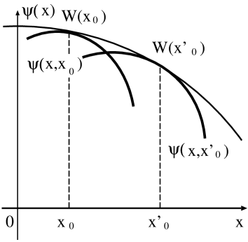
Fig. 1: The local solutions and the global solution as their envelope.

The above program can be performed as follows. The decisive observation is that the lowest order solution may be written as

$$\varphi_{0}(x;x_{0})=Z(x_{0})e^{-x^{2}/4},$$ (3.10)

with an arbitrary function $Z(x_{0})$ of $x_{0}$. We remark that the $E_{0}=1/2$ in this case, too. Accordingly, the boundary value is

$$W_{0}(x_{0})=Z(x_{0})e^{-x_{0}^{2}/4}.$$ (3.11)

The higher order terms may be written as

$$\varphi_{n}(x;x_{0})=Z(x_{0})e^{-x^{2}/4}Q_{n}(x;x_{0}),$$ (3.12)

where $Q_{n}(x;x_{0})$ is a polynomial of $x$, dependent on $x_{0}$. $Q_{n}(x;x_{0})$ is found to satisfy the same recursion relation Eq.(3.5) as $P_{n}(x)$. We impose the boundary condition (B.C.) as

$$\varphi_{n}(x_{0};x_{0})=W_{n}(x_{0})=0\ \ \ {\rm or}\ \ \ Q_{n}(x_{0};x_{0})=0,$$ (3.13)

for $n\geq 1$ because we want to make the lowest order solution as close as the exact one at $x=x_{0}$. Thus one readily obtains

$$Q_{1}(x;x_{0})=P_{1}(x)-P_{1}(x_{0}),.$$ (3.14)

We remark that a constant is the solution of the homogeneous equation. The second order equation reads

$$Q_{2}^{\prime\prime}(x;x_{0})-xQ_{2}^{\prime}(x;x_{0}) = \bigl{(}\frac{x^{4}}{4}P_{1}(x)-\sum_{j=0}^{2}P_{j}(x)E_{n-j}\bigl{)}$$

$$-P_{1}(x_{0})({x^{4}}/{4}-E_{1}).$$ (3.15)

One can verify that $E_{2}$ is given by Eq.(3.6). Since Eq.(3.15) is a linear equation and the inhomogeneous part is a linear combination of those for $P_{2}(x)$ and $P_{1}(x)$, $Q_{2}(x;x_{0})$ satisfying (3.13) is given by

$$Q_{2}(x;x_{0})=(P_{2}(x)-P_{2}(x_{0}))-P_{1}(x_{0})(P_{1}(x)-P_{1}(x_{0})).$$ (3.16)

Repeating the procedure, one finds that $Q_{n}(x;x_{0})$ are expressed in terms of $P_{j}(x)$ ($j\leq n$); see Ref. ? for the explicit forms for $n\leq 6$.

Thus we obtain the approximate solution valid around $x\sim x_{0}$,

$$\psi(x;x_{0})\sim Z(x_{0})e^{-x^{2}/4}\sum_{n=0}^{\infty}\epsilon^{n}Q_{n}(x;x_{0}),$$ (3.17)

where

$$\psi(x_{0};x_{0})=W_{0}(x_{0})=Z(x_{0})e^{-x_{0}^{2}/4}.$$ (3.18)

Now we have obtained a family of curves $\{\psi(x;x_{0})\}_{x_{0}}$ with $x_{0}$ parametrizing the curves; each curve is a good approximation for $x$ around $x_{0}$. The envelope of the local solutions is giving by solving the following equation,

$$\frac{d\psi(x;x_{0})}{dx_{0}}\Bigl{|}_{x_{0}=x}=0,$$ (3.19)

which is in the same form as the renormalization group equation; one may have called it the RG equation. The equation gives a condition which $Z(x_{0})$ must satisfy;

$$\frac{dZ}{dx}=Z(x)\frac{d}{dx_{0}}\sum_{n=0}^{\infty}\epsilon^{n}(-Q_{n}(x;x_{0}))\Bigl{|}_{x_{0}=x}.$$ (3.20)

Defining $f_{n}(x)$ by

$$-\frac{d}{dx_{0}}Q_{n}(x;x_{0})\bigl{|}_{x_{0}=x}=\frac{df_{n}(x)}{dx},$$ (3.21)

one obtains

$$Z(x)={A}\cdot{\rm exp}[\sum_{n=0}^{\infty}\epsilon^{n}f_{n}(x)],$$ (3.22)

where $A$ is a constant. With this solution, the global solution $\psi_{E}(x)$ is given by the boundary value by construction;

$$\psi_{E}(x)=W_{0}(x) = Z(x)e^{-x^{2}/4}={A}\cdot{\rm exp}[-\frac{x^{2}}{4}+\sum_{n=1}^{\infty}\epsilon^{n}f_{n}(x)].$$ (3.23)

This is one of the main results of the present work.

$f_{n}(x)$’s are easily calculated in terms of $P_{n}(x)$;

$$f_{1}(x) = P_{1}(x)=-\frac{3}{8}x^{2}-\frac{1}{16}x^{4},f_{2}(x)=P_{2}(x)-\frac{1}{2}P_{1}(x)^{2}=\frac{21}{16}x^{2}+\frac{11}{64}x^{4}+\frac{1}{96}x^{6},$$

$$f_{3}(x) = P_{3}(x)-P_{1}(x)P_{2}(x)+\frac{1}{3}P_{1}(x)^{3}=-\frac{333}{32}x^{2}-\frac{45}{32}x^{4}-\frac{21}{192}x^{6}-\frac{1}{256}x^{8},$$

$$f_{4}(x) = P_{4}(x)-P_{1}(x)P_{2}(x)-\frac{1}{2}P_{2}(x)^{2}+P_{1}(x)^{2}P_{2}(x)-\frac{1}{4}P_{1}(x)^{4},$$

$$= \frac{30885}{256}x^{2}+\frac{8669}{512}x^{4}+\frac{1159}{768}x^{6}+\frac{163}{2048}x^{8}+\frac{x^{10}}{512},$$

$$f_{5}(x) = P_{5}(x)-P_{1}(x)P_{4}(x)-P_{2}(x)P_{3}(x)+P_{1}(x)P_{2}(x)^{2}-P_{1}(x)^{3}P_{2}(x)$$

$$+P_{1}(x)^{2}P_{3}(x)+\frac{1}{5}P_{1}(x)^{5},$$

$$= -\frac{916731}{512}x^{2}-\frac{33171}{128}x^{4}-\frac{6453}{256}x^{6}-\frac{823}{512}x^{8}-\frac{319}{5120}x^{10}-\frac{7}{6144}x^{12},$$

$$f_{6}(x) = P_{6}(x)-P_{1}(x)P_{5}(x)-P_{2}(x)P_{4}(x)+P_{1}(x)^{2}P_{4}(x)-\frac{1}{2}P_{3}(x)^{2}+2P_{1}(x)P_{2}(x)P_{3}(x)$$

$$-P_{1}(x)^{3}P_{3}(x)+\frac{1}{3}P_{2}(x)^{3}-\frac{3}{2}P_{1}(x)^{2}P_{2}(x)^{2}+P_{1}(x)^{4}P_{2}(x)-\frac{1}{6}P_{1}(x)^{6},$$

$$= \frac{65518401}{2048}x^{2}+\frac{19425763}{4096}x^{4}+\frac{752825}{1536}x^{6}+\frac{43783}{4096}x^{8}+\frac{3481}{2048}x^{10}+\frac{1255}{24576}x^{12}$$

$$+\frac{3}{4096}x^{14},$$ (3.24)

and so on. $f_{1}(x)\sim f_{3}(x)$ coincide with the results in Ref. 10), where explicit expressions of $f_{n}(x)$ are given only for $n\leq 3$. It is interesting that the polynomials $f_{n}(x)$ are given in terms of $P_{n}(x)$ appearing in the naive perturbative expansion in a closed form. It should be instructive to remark here that $f_{i}(x)$’s ($i=1,2,3,...$) are the cumulant[16] of the sum $\sum_{n=0}^{\infty}\epsilon^{n}P_{n}(x)$ in the sense that

$$\sum_{n=0}^{\infty}\epsilon^{n}P_{n}(x)\sim{\rm exp}[\sum_{n=0}^{\infty}\epsilon^{n}f_{n}(x)].$$ (3.25)

In short, the RG method based on the construction of an envelope certainly resumes the perturbation series of the wave function and the resultant expression are given in terms of the cumulants of the naive perturbation series. Conversely, our method provides a mechanical way for computing cumulants of given series.

3.3 Reproducing the WKB result

We now examine how the WKB result Eq.(3.2) can be reproduced from the perturbation series obtained above. Bender and Bettencourt found that if all terms beyond $1/512\cdot\epsilon^{4}x^{10}$ are neglected, the sum of the highest power terms in $f_{j}(x)$ $(j\leq 4)$ is nicely rewritten as $-{x^{2}}/{4}(1+2\epsilon x^{2}+{17}/{12}\cdot\epsilon^{2}x^{4}+{5}/{12}\cdot\epsilon^{3}x^{6}+{47}/{1152}\cdot\epsilon^{4}x^{8})^{1/8}$, which behaves for large $x$ as

$$-\sqrt{\epsilon}|x|^{3}/4(1152/47)^{1/8}\simeq\sqrt{\epsilon}|x|^{3}/5.96663,$$ (3.26)

in an excellent agreement with the WKB result. How about the higher orders. In the fifth order, the sum of the highest powers may be rewritten by neglecting all terms beyond $7\epsilon^{5}x^{10}/1286$ as $-{x^{2}}/{4}\cdot(1+\epsilon x^{2}/4-\epsilon^{2}x^{4}/24+\epsilon^{3}x^{6}/64-\epsilon^{4}x^{8}/128+7\epsilon^{5}x^{10}/1286)$ $\sim-{x^{2}}/{4}(1+{5}/{2}\cdot\epsilon x^{2}+{115}/{48}\cdot\epsilon^{2}x^{4}+{35}/{32}\cdot\epsilon^{3}x^{6}+{15}/{64}\cdot\epsilon^{4}x^{8}+{4459}/{164608}\cdot\epsilon^{5}x^{10})^{1/10}$. For large $x$, the coefficient of $-\sqrt{\epsilon}|x|^{3}$ is $4(164608/4459)^{1/10}\simeq 5.73827$, which deviates from 6 more than the fourth order result. Unfortunately, the sixth order becomes worse: The sum of the highest powers is rewritten as $-{x^{2}}/{4}(1+3\epsilon x^{2}+{29}/{8}\cdot\epsilon^{2}x^{4}+{9}/{4}\cdot\epsilon^{3}x^{6}+{577}/{768}\cdot\epsilon^{4}x^{8}+{67621}/{493824}\cdot\epsilon^{5}x^{10}+{1324349}/{35555328}\cdot\epsilon^{6}x^{12})^{1/12}$, which makes the coefficient of $-\sqrt{\epsilon}|x|^{3}$ for large $x$

$$4(35555328/1324349)^{1/12}\simeq 5.26181.$$ (3.27)

This is actually plausible because the convergence radius of the perturbation series is zero; the cumulant series should be at best an asymptotic series.

4 Summary and Concluding Remarks

In summary, we have successfully applied the RG method[2] as formulated in Ref. ?, ? to Schrödinger equation of the quantum anharmonic oscillator: The naive perturbation series of the wave function are resummed by the RG equation. We have found the following: Although the sum of the highest power in $f_{n}(x)$ can be organized so that it becomes asymptotically proportional to $\sqrt{\epsilon}|x|^{3}$ as was done in [10, 12], the coefficient of it reaches the closest value to 6, the WKB result, in the fourth order, then goes away monotonously from the closest value in the higher orders. We remark that the RG method as developed here can be also applied to the first excited state.

It should be stressed that the method presented here can improve perturbative wave functions for all cases where naive perturbative solutions of Bender-Wu type are given; namely, the RG method combined with the Bender-Wu perturbation method constitutes a new powerful method for improving perturbative wave functions. It is interesting to extend the present method and apply it to quantum field theory, although it has been indicated that the notion of envelopes is useful for improving the effective potential given in the loop expansion.[4]

The present RG method is an application of the perturbative RG equation. Can nonperturbative RG equations be useful to construct global wave functions? It should be. Indeed a variational method called the delta-expansion method[18] which also utilizes an RG-like equation but nonperturbatively has been extended for obtaining wave functions.[19] The key ingredient of the extension is to construct an envelope of a set of perturbative wave functions as in the RG method but with a variational parameter. In this method, although the basic equation can not be solved analytically but only numerically, uniformly valid wave functions with correct asymptotic behavior are obtained in the first-order perturbation even for strong couplings and for excited states. In the present method, the basic equations are solved analytically, and the asymptotic form of the wave function is constructed explicitly, although a further resummation devised in [10, 12] is needed for obtaining the asymptotic form. In this sense, the two methods are complementary to each other. It would be interesting if one can combine the two methods.

References

-
[1]
E.C.G. Stuckelberg and A. Petermann, Helv. Phys. Acta
26(1953), 499.
M. Gell-Mann and F. E. Low, Phys. Rev. 95 (1953), 1300.
See also K. Wilson,Phys. Rev. D3 (1971), 1818,
S. Weinberg, in Asymptotic Realms of Physics, ed. A. H. Guth et al. (MIT Press, 1983); The Quantum Theory of Fields, vol. II, chap. 18, (Cambridge University Press, 1996). - [2] N. Goldenfeld, O. Martin and Y. Oono, J. Sci. Comp. 4(1989),4; N. Goldenfeld, O. Martin, Y. Oono and F. Liu, Phys. Rev. Lett. 64(1990), 1361; N. D. Goldenfeld, Lectures on Phase Transitions and the Renormalization Group (Addison-Wesley, Reading, Mass., 1992); L. Y. Chen, N. Goldenfeld, Y. Oono and G. Paquette, Physica A 204(1994), 111; G. Paquette, L. Y. Chen, N. Goldenfeld and Y. Oono, Phys. Rev. Lett. 72(1994),76; L.-Y. Chen, N. Goldenfeld and Y. Oono, Phys. Rev. Lett. 73(1994),1311; Phys. Rev. E 54(1996),376.
- [3] C. M. Bender and S. A. Orszag, Advanced Mathematical Methods for Scientists and Engineers (McGraw-Hill, New York, 1978).
- [4] T.Kunihiro, Prog. Theor. Phys. 94 (1995), 503; (E) 95 (1996), 835; Jpn. J. Ind. Appl. Math. 14(1997),51.
- [5] T. Kunihiro, Prog. Theor. Phys. 97(1997),179; see also, patt-sol/9709003, on which §§2.1 of the present report is based.
-
[6]
S. Coleman and E. Weinberg, Phys. Rev. D7 (1973), 1888;
M. Sher, Phys. Rep. 179 (1989),274.
M. Bando, T.Kugo, N. Maekawa and H. Nakano, Phys. Lett. B301 (1993), 83; Prog. Theor. Phys. 90 (1993), 405.
C. Ford, Phys. Rev. D50 ( 1994), 7531.
H. Nakkagawa and H. Yokota, Modern Phys. Lett. A 11 (1996), 2259. - [7] D. V. Shirkov, Russian Math. Surveys 49: 5 (1994),155; hep-th/9602024; V. F. Kovalev, V. V. Pustovalov and D. V. Shirkov, hep-th/9706056 to be published in J. Math. Phys.
-
[8]
Large Order Behavior of Perturbation Theory,
Current Physics – Sources and Comments, vol.7,
ed. J. C. Le Guillou and J. Zinn-Justin, (North-Holland, Amsterdam, 1990).
G. A. Arteca, F. M. Fernández and E. A. Castro, Large Order Perturbation Theory and Summation Methods in Quantum Mechanics, (Springer-Verlag, Berlin, 1990). - [9] T. Kunihiro, Phys. Rev. D57(1998),.
- [10] C. M. Bender and L. M. A. Bettencourt, Phys. Rev. Lett. 77(1996), 4114; Phys. Rev. D54(1996), 7710.
- [11] M. Frasca, Nuovo Cimento, B107(1992),915; 109(1994),603.
- [12] C. A. Ginsburg and E. W. Montroll, J. Math. Phys. 19(1978),336.
- [13] I. L. Egusquiza and M. A. Valle Basagoiti, Report NO. hep-th/9611143, 1996.
- [14] M. Frasca, Phys. Rev. A 56(1997),1548.
-
[15]
R. Graham, Phys. Rev. Lett. 76 (1996), 2185.
S. Sasa, Physica D108(1997),45.
H.J. de Vega and J.F.J Salgado, Phys. Rev. D56 (1997),6524.
T. Kunihiro and J. Matsukidaira, Phys. Rev. E57 (1998), . - [16] For example, see R. Kubo, M. Toda and N. Hashitsume, Statistical Physics II Nonequilibrium Statistical Mechanics, 2nd ed. (Springer 1995).
- [17] C. M. Bender and T. T. Wu, Phys. Rev. 184(1969),1231; ibid. D7(1973),1620.
-
[18]
P. M. Stevenson, Phys. Rev. D23(1981),2916.
C. Arvanitis, H. F. Jones and C. S. Parker, Phys. Rev. D52 (1995),3704.
H. Kleinert, Path Integrals in Quantum Mechanics, Statistical and Polymer Physics, 2nd. edition (World Scientific, Singapore, 1995), and references cited therein.
E. J. Weniger, Phys. Rev. Lett. 77(1996), 2859.
R. Guida, K. Konishi and H. Suzuki, Ann. Phys. 241 (1995),152; ibid. 249(1996),109. -
[19]
T. Hatsuda, T. Kunihiro and T. Tanaka,
Phys. Rev. Lett. 78(1997),3229; T. Tanaka, Phys. Lett. A ( 1998), .
S. K. Kauffman and S. M. Perez, J. Phys. A 17 (1984),2027; ibid., A19(1986), 3807.