Unoriented Open-Closed String Field Theory

1 Introduction

The discovery of D-branes[1] has brought us with a quite new insight into string theories and various duality properties there, and actually triggered the recent rapid developments in the fields. Now the string theory seems no longer the theory of string alone, but the theory for a totality of branes with various dimensional extension.

The most remarkable one among the recent developments would be matrix theory formulations for such a ‘string theory’,[2, 3] in which the various dimensional branes seems to be described unifiedly by a very simple looking system of matrix variables. It may also suggest a possibility for a quite new formulation for the ‘second-quantized theory’ of many body systems in place of the conventional field theory. There are, however, many subtle problems in the limiting procedure of $N\rightarrow\infty$ and it is still lacking some key idea for the matrix theory to become a truly powerful ‘second quantized theory’ by which the conventional field theory can be a replaced. We still have something to learn from the conventional field theory.

Despite these developments the dynamics of the D-branes does not seem fully made clear. At this stage it would be necessary to try various approaches to reveal the string dynamics, namely, of various branes. There already appears some trials for studying the string system with D-branes in terms of string field theories. One approach by Hashimoto and Hata[4] is to introduce the D-brane explicitly in the closed string field theory as a source term using the boundary state. Another approach by Zwiebach,[5] who worked in the non-polynomial string field theory framework, is based on oriented open-closed string field theory, in which D-branes were not directly introduced but it is described by the end points of the open string by performing the T-duality transformation.

The purpose of this paper is to construct the string field theory for unoriented open-closed string mixed system with joining-splitting type vertices and to reveal the gauge symmetry structure. This is of course in the hope to study the D-brane dynamics eventually. In open-closed string theories, the unoriented Type I theory with gauge group $SO(32)$ is the only known consistent one. Unless the gauge group is $SO(32)$, the anomaly dose not cancel, and the infinities coming from the dilaton tadpole do appear so that the supersymmetric vacuum becomes unstable.[6, 7]   In bosonic case also, the infinities of the dilaton tadpole are known to be canceled if and only if the gauge group is $SO(2^{13}=8192)$ in the unoriented theory.[8]  Therefore, we can naturally expect that this infinity cancellation mechanism also work to guarantee the gauge invariance of the open-closed string field theory.

Since the bosonic string theories always suffer from the tachyon problem, we should ideally treat supersymmetric string theories. But, at the present stage, there are still difficult problems for constructing supersymmetric string field theories.[9, 10]   So we here have to content ourselves with the construction of bosonic string field theory for the unoriented open-closed mixed system with gauge group SO($n$). Moreover, in this open-closed mixed system, there is an anomaly for the gauge transformation with open-string field parameter, which is similar to more familiar Lorentz anomaly in the light-cone gauge string field theory.[11, 12, 13]  Since we need a bit complicated loop amplitude calculations to treat it, we defer the discussion of the open-string parameter gauge transformation to the forthcoming paper.[14]  In this paper, we treat only the gauge transformation with closed string field parameter restricting the action to the quadratic part in the string fields.

In the unoriented open-closed string field theory, there are three type of vertices for quadratic interactions as drawn in Fig. 3. One of them, $U$, corresponds to the transition from open to closed string, and vice versa. The others, $V_{\propto}$ and $V_{\infty}$, are the vertices in which an open or closed string intersects itself and rearranges. So, we can write the quadratic part of the action in the form:

$$S = -\hbox{${1\over 2}$}\mathchar 28937\relax{\hskip 1.0pt{\cdot}\hskip 1.0pt}{\tilde{Q}}_{\rm B}\mathchar 28937\relax-\hbox{${1\over 2}$}\mathchar 28936\relax{\hskip 1.0pt{\cdot}\hskip 1.0pt}{\tilde{Q}}_{\rm B}b_{0}^{-}\mathchar 28936\relax$$ (1.1)

$$\qquad+x_{u}g\,\mathchar 28937\relax{\hskip 1.0pt{\cdot}\hskip 1.0pt}U\mathchar 28936\relax+x_{\propto}\,\frac{g^{2}}{2}\,\mathchar 28937\relax{\hskip 1.0pt{\cdot}\hskip 1.0pt}V_{\propto}\mathchar 28937\relax+x_{\infty}\,\frac{g^{2}}{2}\,\mathchar 28936\relax{\hskip 1.0pt{\cdot}\hskip 1.0pt}V_{\infty}\mathchar 28936\relax,$$

where $\mathchar 28937\relax$ and $\mathchar 28936\relax$ denote open and closed string field, respectively, and $x_{u}$, $x_{\propto}$ and $x_{\infty}$ are coupling constants (relative to the open 3-vertex coupling constant $g$) for the open-closed transition $U$, open intersection $V_{\propto}$ and closed intersection $V_{\infty}$ interactions, respectively. The details of the definition will be explained in the text.

We consider the following form of gauge transformation with a closed string field parameter $\mathchar 28931\relax^{\mathrm{c}}$:

$$\delta(b_{0}^{-}\mathchar 28936\relax) = -{\tilde{Q}}_{\rm B}b_{0}^{-}\mathchar 28931\relax^{\mathrm{c}}+x_{\infty}g^{2}V_{\infty}\,\mathchar 28931\relax^{\mathrm{c}},$$

$$\delta\mathchar 28937\relax = x_{u}gU\mathchar 28931\relax^{\mathrm{c}},$$ (1.2)

where $\mathchar 28931\relax^{\mathrm{c}}$ denotes a functional of closed string coordinate. Under this transformation, the action of Eq. (1.1) is transformed, roughly writing, as

$$\delta S = \mathchar 28936\relax\cdot{\tilde{Q}}_{\rm B}^{2}b_{0}^{-}\mathchar 28931\relax^{\mathrm{c}}+x_{u}g\,\mathchar 28937\relax\cdot[{\tilde{Q}}_{\rm B},\,U]\mathchar 28931\relax^{\mathrm{c}}+g^{2}\,\mathchar 28936\relax\cdot\left(x_{u}^{2}\,UU-x_{\infty}\,\{{\tilde{Q}}_{\rm B},\,{V}_{\infty}\}\right)b_{0}^{-}\mathchar 28931\relax^{\mathrm{c}}$$ (1.3)

$$+x_{u}g^{3}\,\mathchar 28937\relax\cdot\left(-x_{\infty}\,{U}V_{\infty}+x_{\propto}\,V_{\propto}U\right)\mathchar 28931\relax^{\mathrm{c}}-x_{\infty}g^{4}\,\mathchar 28936\relax\cdot{V}_{\infty}V_{\infty}\mathchar 28931\relax^{\mathrm{c}}.$$

In order to realize the gauge invariance, each term of Eq. (1.3) must vanish order by order. Moreover, in $O(g^{2})$ terms in Eq. (1.3), the first $UU$ term corresponds to a singular world sheet of a disk and the second $\{{\tilde{Q}}_{\rm B},\,{V}_{\infty}\}$ term to real projective ($RP^{2}$) plane, each with two external states. They both contain infinities due to the dilaton and tachyon contributions in the configuration drawn in Fig. 5.2 below. Thus, the unoriented open-closed string field theory can be gauge invariant if and only if the infinity cancellation occurs between the disk and $RP^{2}$ amplitudes. Conversely speaking, in the case of oriented open-closed string field theory, there is no $RP^{2}$ contribution since it comes from the $V_{\infty}$ vertex characteristic to the unoriented string, and therefore it requires other novel infinity cancellation mechanism [15] in order for the oriented string theory to be gauge invariant. This point is also the problem for the Lorentz invariance in the light-cone gauge string field theory of oriented open-closed strings, which seems to have not been noticed by other authors up to now.[11, 12, 13]

This paper is organized as follows. In sect. 2, we fix our conventions and notations for string fields as well as string coordinates as conformal fields. In sects. 3 and 4, we give precise definitions for the above vertices and action. In sect. 5, we prove the gauge invariance of the quadratic action for unoriented open-closed string field theory and determine relations between various coupling constants to satisfy the gauge invariance. Then, in sect. 6, we calculate two closed tachyon amplitudes corresponding to the disk and $RP^{2}$ from string field theory action, and see that the infinity cancellation occurs if and only if the gauge invariance condition is met. Sect. 7 is devoted to the summary and some more discussions on the gauge symmetry. Appendix A is added for clarifying the relations between three different expressions for the vertices by LeClair, Peskin and Preitschopf (LPP),[16] Kunitomo and Suehiro (KS),[17] and Hata, Itoh, Kugo, Kunitomo and Ogawa (HIKKO),[18, 19] which is necessary for the gauge-invariance proof in Sect. 5. Appendix B gives the explicit formula for the Neumann coefficients of open-closed transition vertex.

2 String Fields

Let us recall the mode expansion of string coordinates $\phi\equiv(X^{\mu},\ c,\ b)$ and fix our convention. In a unit disk $\left|w_{r}\right|\leq 1$, the string coordinates are expanded as

$$X^{\mu}(w_{r})=x^{\mu}-i\,\alpha_{0}^{\mu}\ln w_{r}+i\sum_{n\neq 0}\frac{1}{n}\alpha^{\mu}_{n}w_{r}^{-n},$$

$$c(w_{r})=\sum_{n}c_{n}w_{r}^{-n+1},\qquad b(w_{r})=\sum_{n}b_{n}w_{r}^{-n-2},$$

$$[x^{\mu},\,\alpha^{\nu}_{0}]=i\eta^{\mu\nu},\qquad\eta^{\mu\nu}={\rm diag}(-1,+1,\cdots,+1),$$ (2.1)

where $r$ denotes $r$-th string and $l_{s}=\sqrt{2\alpha^{\prime}}$ is set equal to 1. There is also an anti-holomorphic counterpart $\bar{\phi}(\bar{w}_{r})=(\bar{X}^{\mu}(\bar{w}_{r}),\ \bar{c}(\bar{w}_{r}),\ \bar{b}(\bar{w}_{r}))$ for closed string, which lives in the unit disk with anti-holomorphic coordinate $\bar{w}_{r}$, $|\bar{w}_{r}|\leq 1$. For any conformal mapping $z\rightarrow z^{\prime}$, the string coordinates $\phi(z)$ are mapped as follows according to their conformal weights $d_{\phi}=(0,\ -1,\ +2)$ for $\phi=X^{\mu},c,b$:

$$\phi(z)\rightarrow\phi^{\prime}(z^{\prime})=\left({dz\over dz^{\prime}}\right)^{d_{\phi}}\phi(z).$$ (2.2)

The unit disk can of course be mapped to a semi-infinite cylinder with more familiar world-sheet coordinate $\rho_{r}=\tau_{r}+i\sigma_{r}$, $\tau_{r}\leq 0$ by a conformal mapping $w_{r}=e^{\rho_{r}}=e^{\tau_{r}+i\,\sigma_{r}}$, and the string coordinates on the $\rho_{r}$ plane are therefore given by

$$X^{\mu}(\rho_{r})=x^{\mu}-i\,\alpha_{0}^{\mu}\rho_{r}+i\sum_{n\neq 0}\frac{1}{n}\alpha^{\mu}_{n}e^{-n\rho_{r}},$$

$$c(\rho_{r})=\sum_{n}c_{n}e^{-n\rho_{r}},\qquad b(\rho_{r})=\sum_{n}b_{n}e^{-n\rho_{r}}.$$ (2.3)

For open-string, the $\sigma_{r}$ originally runs only over $0\leq\sigma_{r}\leq\pi$, but it is extended in these equations to run over $0\leq\sigma_{r}\leq 2\pi$ just as for the closed string. Because of $2\pi$ periodicity of $\sigma_{r}$, we shall conveniently take also the region $-\pi\leq\sigma_{r}\leq\pi$ as well as $0\leq\sigma_{r}\leq 2\pi$ as the fundamental region of $\sigma_{r}$ both for open and closed strings, depending on the situations. Note also that the real string coordinate $X^{\mu}(\sigma,\tau)$ is given by

$$X^{\mu}(\sigma,\tau)=\hbox{${1\over 2}$}{\hbox{$\left(\vbox to0.0pt{}\right.\n@space$}}X^{\mu}(\rho)+\bar{X}^{\mu}(\bar{\rho}){\hbox{$\left)\vbox to0.0pt{}\right.\n@space$}}$$ (2.4)

with the understanding that $\bar{X}^{\mu}=X^{\mu}$ for open string case.

The open string field $\mathchar 28937\relax$ and closed one $\mathchar 28936\relax$ are denoted in our notation by

$$\left|\mathchar 28937\relax\right> = \left|\phi\right>+c_{0}\left|\psi\right>,$$

$$\left|\mathchar 28936\relax\right> = c_{0}^{-}\left(\left|\phi\right>+c_{0}^{+}\left|\psi\right>\right)+\left(\left|\chi\right>+c_{0}^{+}\left|\eta\right>\right).$$ (2.5)

It should be kept in mind that the open string field is $n\times n$ matrix valued; $\left|\mathchar 28937\relax\right>_{ij}$. As for the ghost zero-modes for the closed string, we use the notation:

$$c_{0}^{+}\equiv\hbox{${1\over 2}$}(c_{0}+\bar{c}_{0}),\quad c_{0}^{-}=c_{0}-\bar{c}_{0},$$

$$b_{0}^{+}\equiv b_{0}+\bar{b}_{0},\quad b_{0}^{-}\equiv\hbox{${1\over 2}$}(b_{0}-\bar{b}_{0}).$$ (2.6)

The physical fields are contained in the $\left|\phi\right>$ component. We take the $\left|\phi\right>$ component to be Grassmann even, so that the closed string field $\left|\mathchar 28936\relax\right>$ is Grassmann odd while the open string field $\left|\mathchar 28937\relax\right>$ is even. We define the Fock vacuum $\left|1\right>=(\langle 1|)^{\dagger}$ by

$$\alpha_{n}^{\mu}\left|1\right> = 0\quad{\rm for}\ \ n\geq 1,$$

$$c_{n}\left|1\right> = 0\quad{\rm for}\ \ n\geq 1,$$

$$b_{n}\left|1\right> = 0\quad{\rm for}\ \ n\geq 0,$$ (2.7)

and we keep to use the coordinate (or momentum) representation for the zero modes $p^{\mu}$, $x^{\mu}$. $\left|1,1\right>=(\langle 1,1|)^{\dagger}$ is the Fock vacuum for the closed string possessing the holomorphic and anti-holomorphic oscillator freedoms. Concerning the ghost mode part, in particular, the Fock vacuum is related with the conformal vacuum $\left|0\right>$ by

$$\left|1\right>=c_{1}\left|0\right>,\quad\langle 1|=\langle 0|c_{-1},\quad\hbox{so that}\quad\langle 1|c_{0}\left|1\right>=\langle 0|c_{-1}c_{0}c_{1}\left|0\right>=1.$$ (2.8)

The label 1 of the Fock vacuum $\left|1\right>$, thus, implies the ghost number relative to the conformal vacuum. As for the order of the holomorphic and anti-holomorphic ghost zero-modes for the closed string case, we take a convention

$$\langle 1,1|c_{0}^{-}c_{0}^{+}\left|1,1\right>=\langle 1,1|c_{0}\bar{c}_{0}\left|1,1\right>=1.$$ (2.9)

We here define reflectors,[20] which convert the ket representation to the bra representation, for the open and closed strings, respectively:

$$\langle R^{\mathrm{o}}(1,2)| = \delta(1,2)\,{\textstyle{\atop 1}}\!\langle 1|{\textstyle{\atop 2}}\!\langle 1|({c_{0}}^{(1)}\!+{c_{0}}^{(2)})\exp{(E^{\mathrm{o}}_{12})},$$

$$\langle R^{\mathrm{c}}(1^{\mathrm{c}},2^{\mathrm{c}})| = \delta(1,2)\,{\textstyle{\atop 1}}\!\langle 1,1|{\textstyle{\atop 2}}\!\langle 1,1|(c_{0}^{+(1)}\!+c_{0}^{+(2)})(c_{0}^{-(1)}\!+c_{0}^{-(2)})\exp{(E^{\mathrm{c}}_{12})},\hskip 20.00003pt$$ (2.10)

with the exponents given by

$$E^{\mathrm{o}}_{12} = \sum_{n\geq 1}(-)^{n+1}\left(\frac{1}{n}{\alpha_{n}^{\mu}}^{(1)}{\alpha_{n}}_{\mu}^{(2)}+{c_{n}}^{(1)}{b_{n}}^{(2)}-{b_{n}}^{(1)}{c_{n}}^{(2)}\right),$$

$$E^{\mathrm{c}}_{12} = -\sum_{n\geq 1}\left(\frac{1}{n}{\alpha_{n}^{\mu}}^{(1)}{\alpha_{n}}_{\mu}^{(2)}+{c_{n}}^{(1)}{b_{n}}^{(2)}-{b_{n}}^{(1)}{c_{n}}^{(2)}\right)+{\rm a.h.},$$ (2.11)

and the delta functions by

$$\delta(1,2,\cdots,n)=(2\pi)^{d}\,\delta^{d}(\sum^{n}_{r=1}p_{r}^{\mu})$$ (2.12)

with $d=26$. We understood that the delta function $\delta(1,2)$ in $\langle R^{\mathrm{o}}(1,2)|$ case also implies the matrix reflection $\delta(i_{1},j_{1};i_{2},j_{2})\equiv\delta_{i_{1},j_{2}}\delta_{i_{2},j_{1}}$. We also define ket reflectors $\left|R^{{\mathrm{o}},{\mathrm{c}}}\right>$ as the inverse of the bra reflectors $\langle R^{{\mathrm{o}},{\mathrm{c}}}|$ in the sense that

$$\langle R^{\mathrm{o}}(1,3)|\left|R^{\mathrm{o}}(3,2)\right>\left|\mathchar 28937\relax\right>_{1}=\left|\mathchar 28937\relax\right>_{2},\quad{\rm for}\ \ \forall\mathchar 28937\relax,$$

$$\langle R^{\mathrm{o}}(1^{\mathrm{c}},3^{\mathrm{c}})|\left|R^{\mathrm{o}}(3^{\mathrm{c}},2^{\mathrm{c}})\right>\left|\mathchar 28936\relax\right>_{1^{\mathrm{c}}}=\left|\mathchar 28936\relax\right>_{2^{\mathrm{c}}}\quad{\rm for}\ \ \forall\mathchar 28936\relax,$$ (2.13)

where the inner-product of the bra and ket states implies, in addition to the usual product for oscillators, integration over the zero-modes, $\int d^{d}p/(2\pi)^{d}$ (as well as the trace operation over the matrix for the open string case). The ket reflectors are easily seen to be the minus of the hermitian conjugates of the bra reflectors:

$$\left|R^{\mathrm{o}}(1,2)\right>=-\left(\langle R^{\mathrm{o}}(2,1)|\right)^{\dagger},\qquad\left|R^{\mathrm{c}}(1^{\mathrm{c}},2^{\mathrm{c}})\right>=-\left(\langle R^{\mathrm{c}}(2^{\mathrm{c}},1^{\mathrm{c}})|\right)^{\dagger}.$$ (2.14)

We note the symmetry property of the reflectors:

$$\langle R^{\mathrm{o}}(2,1)|\left|\mathchar 28937\relax\right>_{1}\left|\mathchar 28937\relax^{\prime}\right>_{2}=-(-1)^{|\mathchar 28937\relax||\mathchar 28937\relax^{\prime}|}\langle R^{\mathrm{o}}(1,2)|\left|\mathchar 28937\relax^{\prime}\right>_{2}\left|\mathchar 28937\relax\right>_{1},$$

$$\langle R^{\mathrm{c}}(2^{\mathrm{c}},1^{\mathrm{c}})|\left|\mathchar 28936\relax\right>_{1}\left|\mathchar 28936\relax^{\prime}\right>_{2}=(-1)^{|\mathchar 28936\relax||\mathchar 28936\relax^{\prime}|}\langle R^{\mathrm{o}}(1^{\mathrm{c}},2^{\mathrm{c}})|\left|\mathchar 28936\relax^{\prime}\right>_{2}\left|\mathchar 28936\relax\right>_{1},$$ (2.15)

where $|\mathchar 28937\relax|$ is 0 (1) if $\left|\mathchar 28937\relax\right>$ is Grassmann even (odd). The minus sign for the former comes from the interchange of the bra Fock vacua: ${\textstyle{\atop 2}}\!\langle 1|{\textstyle{\atop 1}}\!\langle 1|=-{\textstyle{\atop 1}}\!\langle 1|{\textstyle{\atop 2}}\!\langle 1|$, which effectively contains the ghost zero-mode integration $\int dc_{0}^{(2)}dc_{0}^{(1)}=-\int dc_{0}^{(1)}dc_{0}^{(2)}$.

In defining string vertices below, we assign string length $\alpha$ to each participating string. Basically we adopt in this paper the so-called $\alpha=p^{+}$ HIKKO theory,[20] in which we identify the string length $\alpha$ as follows:

$$\alpha=\cases{2p^{+}&for open string\cr p^{+}&for closed string.\cr}$$ (2.16)

So the $\alpha$ parameter is not an independent freedom unlike in HIKKO theory. (The following discussion in this paper will, however, be equally valid even when we instead adopt the standpoint of ‘covaliantized light-cone string field theory’[21, 22, 23, 24] provided that we make a suitable re-interpretation like replacing the zero mode variable $p^{\mu}$ by an OSp($d+2|2$) vector.) Since only the ratio of the $\alpha$ parameters is relevant to the vertices, the string length parameter $\alpha$ can be fixed to be $\pm 2$ for open and $\pm 1$ for closed strings, respectively, in this paper where only the quadratic vertices are treated.

3 Vertices

We construct BRS invariant vertices corresponding to three types of interactions following the method of LeClair, Peskin and Preitschopf (LPP).[16]

To define BRS invariant vertices a la LPP, we have to specify the way how to connect the strings: a single $\rho$-plane is constructed by gluing the $\rho_{r}$-planes (or, unit disks $w_{r}$,) of individual strings. In the case of the open-closed transition vertex $U$, the coordinate $\rho$ is identified region-wise with the coordinate of each string, as depicted in Fig. 2:

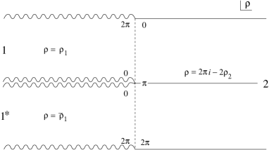
Fig. 2: The $\rho$ plane representing the connection of open-closed transition vertex $U$.

$$\rho=\tau+i\sigma=\cases{\rho_{1}=\tau_{1}+i\sigma_{1}&for $\tau\leq 0$,\ \ $0\leq\sigma\leq 2\pi$ : region 1\cr\bar{\rho}_{1}=\tau_{1}-i\sigma_{1}&for $\tau\leq 0$,\ \ $-2\pi\leq\sigma\leq 0$ : region $1^{*}$\cr-2\rho_{2}+2\pi i&\cr\quad=-2(\tau_{2}+i\sigma_{2})+2\pi i&for $\tau\geq 0$, \ \ $-2\pi\leq\sigma\leq 2\pi$ : region 2.\cr}$$ (3.1)

Note that, as explained before, we have assigned string length parameter $\alpha_{1}=1$ for incoming closed string 1 and $\alpha_{2}=-2$ for outgoing open string 2. The regions 1 and $1^{*}$ stand for the holomorphic and anti-holomorphic parts of the closed string 1, and the region 2 for the open string 2. With this gluing, a single holomorphic function $\phi(\rho)$ is defined on the $\rho$ plane:

$$\phi(\rho)=\cases{\phi^{(1)}(\rho)&in region 1\cr\bar{\phi}^{(1)}(\rho)&in region $1^{*}$\cr(-2)^{-d_{\phi}}\,\phi^{(2)}(-\rho/2+\pi i)&in region 2.\cr}$$ (3.2)

Therefore, considering the overlapping line $\tau=0$ and Eq. (3.2), we have the following connection equations on the LPP vertex for the open-closed transition, $\langle u(2,1^{\mathrm{c}})|$:

$$\langle u(2,1^{\mathrm{c}})|\bigl{[}\phi^{(1)}(i\sigma)-(-2)^{-d_{\phi}}\phi^{(2)}(i\pi-i\sigma/2)\bigr{]}=0,$$

$$\langle u(2,1^{\mathrm{c}})|\bigl{[}\bar{\phi}^{(1)}(-i\sigma)-(-2)^{-d_{\phi}}\phi^{(2)}(i\pi+i\sigma/2)\bigr{]}=0,$$ (3.3)

for $0\leq\sigma\leq 2\pi$. Note that the real coordinate $X^{\mu}(\sigma,\tau)$ at $\tau=0$ is given by $X^{\mu}(\sigma,0)=\hbox{${1\over 2}$}{\hbox{$\left(\vbox to0.0pt{}\right.\n@space$}}X^{\mu}(i\sigma)+\bar{X}^{\mu}(-i\sigma){\hbox{$\left)\vbox to0.0pt{}\right.\n@space$}}$. So $X^{(1)}(\sigma,0)=X^{(2)}(\pi-\sigma/2,0)$ is realized on the vertex $\langle u(2,1^{\mathrm{c}})|$ as desired.

The $\rho$ plane for the open intersection interaction $V_{\propto}$ is a bit more complicated. Prepare the $\rho$ plane first as follows:

$$\rho=\cases{\rho_{1}=\tau_{1}+i\,\sigma_{1}&for $\tau\leq 0$,\ \ $-\pi\leq\sigma\leq\pi$ : region 1\cr-\rho_{2}+\pi i=-(\tau_{2}+i\,\sigma_{2})+\pi i&for $\tau\geq 0$,\ \ $-\pi\leq\sigma\leq\pi$ : region 2.\cr}$$ (3.4)

Then, as shown in Fig. 4, we make two cuts running from $\sigma=\sigma_{1}$ to $\sigma=\sigma_{2}$ and from $\sigma=-\sigma_{2}$ to $\sigma=-\sigma_{1}$ at $\tau=0$. And the left hand side points on the one cut are identified with the right hand side points on the other cut; namely, the point $\sigma\in[\sigma_{1},\,\sigma_{2}]$ at $\tau=0$ in the region 1 (2) is identified with the point $\sigma-(\sigma_{1}+\sigma_{2})\in[-\sigma_{2},\,-\sigma_{1}]$ in the region 2 (1). With this identification through the cuts, the desired $\rho$ plane is defined, as drawn in Fig. 4.

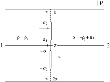
Fig. 3: The $\rho$ plane for open intersection vertex ${V_{\propto}}$.

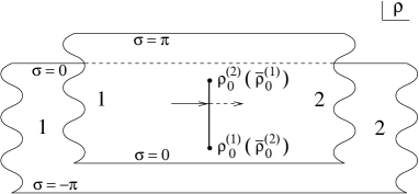
Fig. 4: Redrawing of the $\rho$ plane for the vertex ${V_{\propto}}$ with the cut overlapped. $(\bar{\rho}_{0}^{(i)})$ denotes the branch points on the second sheet.

The single holomorphic field on the $\rho$ plane is defined as usual by

$$\phi(\rho)=\cases{\phi^{(1)}(\rho)&in region 1\cr(-1)^{-d_{\phi}}\,\phi^{(2)}(-\rho+\pi i)&in region 2.\cr}$$ (3.5)

Considering the cut structure of the Riemann surface of $\rho$ and Eq. (3.5), the open intersection vertex, $\langle v_{\propto}|$, satisfies the following connection condition for $0\leq\sigma\leq\pi$,

$$\langle v_{\propto}(1,2)|\bigl{[}\phi^{(1)}(i\sigma)-(-1)^{-d_{\phi}}\,\phi^{(2)}(i\pi-i\sigma)\bigr{]}=0\qquad(\sigma\leq\sigma_{1},\ \ \sigma\geq\sigma_{2}),$$

$$\langle v_{\propto}(1,2)|\bigl{[}\phi^{(1)}(i\sigma)-(-1)^{-d_{\phi}}\,\phi^{(2)}(-i\sigma_{1}-i\sigma_{2}+i\sigma)\bigr{]}=0\ (\sigma_{1}\leq\sigma\leq\sigma_{2}),\hskip 20.00003pt$$ (3.6)

and, for $-\pi\leq\sigma\leq 0$,

$$\langle v_{\propto}(1,2)|\bigl{[}\phi^{(1)}(i\sigma)-(-1)^{-d_{\phi}}\,\phi^{(2)}(-i\pi-i\sigma)\bigr{]}=0\qquad(\sigma\geq-\sigma_{1},\ \ \sigma\leq-\sigma_{2}),$$

$$\langle v_{\propto}(1,2)|\bigl{[}\phi^{(1)}(i\sigma)-(-1)^{-d_{\phi}}\,\phi^{(2)}(i\sigma_{1}+i\sigma_{2}+i\sigma)\bigr{]}=0\ (-\sigma_{2}\leq\sigma\leq-\sigma_{1}).\hskip 20.00003pt$$ (3.7)

These conditions imply that a open string is twisted in the region of $\sigma_{1}<\left|\sigma\right|<\sigma_{2}$.

In the case of the closed intersection vertex $V_{\infty}$, we first prepare two sheets of $\rho$ planes, one for the holomorphic and another for the anti-holomorphic parts, separately:

first sheet

$$\rho=\cases{\rho_{1}=\tau_{1}+i\,\sigma_{1}&for $\tau\leq 0$,\ \ $-\pi\leq\sigma\leq\pi$ : region 1\cr-\rho_{2}=-\tau_{2}-i\,\sigma_{2}&for $\tau\geq 0$,\ \ $-\pi\leq\sigma\leq\pi$ : region 2,\cr}$$

second sheet

$$\rho=\cases{\bar{\rho}_{1}=\tau_{1}-i\,\sigma_{1}&for $\tau\leq 0$,\ \ $-\pi\leq\sigma\leq\pi$ : region $1^{*}$\cr-\bar{\rho}_{2}=-\tau_{2}+i\,\sigma_{2}&for $\tau\geq 0$,\ \ $-\pi\leq\sigma\leq\pi$ : region $2^{*}$.\cr}.$$ (3.8)

Then, again two cuts are placed from $\sigma=-\sigma_{0}$ to $\sigma=+\sigma_{0}$ at $\tau=0$ on the first sheet and on the second as shown in Fig. 6, and again the left hand side points on the one cut are identified with the right hand side points on the other cut. The resulting $\rho$ plane is drawn in Fig. 6.

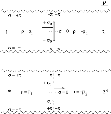
Fig. 5: Two sheets of $\rho$ planes for vertex ${V_{\propto}}$.

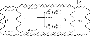
Fig. 6: The $\rho$ plane for the closed intersection vertex ${V_{\propto}}$ drawn in such a way that the cut is overlapped. Again $(\bar{\rho}_{0}^{(i)})$ denotes the coordinates of the branch points on the second sheet.

The holomorphic fields are defined by

$$\phi(\rho)=\cases{\phi^{(1)}(\rho)&in region 1\cr\bar{\phi}^{(1)}(\rho)&in region $1^{*}$\cr(-1)^{-d_{\phi}}\,\phi^{(2)}(-\rho)&in region 2\cr(-1)^{-d_{\phi}}\,\bar{\phi}^{(2)}(-\rho)&in region $2^{*}$.\cr}$$ (3.9)

As in the above case, we obtain the connection equations on the closed intersection vertex $\langle v_{\infty}|$,

$$\cases{\langle v_{\infty}(1,2)|\bigl{[}\phi^{(1)}(i\sigma)-(-1)^{-d_{\phi}}\,\phi^{(2)}(-i\sigma)\bigr{]}=0\cr\vskip 2.15277pt\cr\langle v_{\infty}(1,2)|\bigl{[}\bar{\phi}^{(1)}(-i\sigma)-(-1)^{-d_{\phi}}\,\bar{\phi}^{(2)}(+i\sigma)\bigr{]}=0\cr}\qquad(\left|\sigma\right|\geq\sigma_{0}),$$

$$\cases{\langle v_{\infty}(1,2)|\bigl{[}\phi^{(1)}(i\sigma)-(-1)^{-d_{\phi}}\,\bar{\phi}^{(2)}(-i\sigma)\bigr{]}=0\cr\vskip 2.15277pt\cr\langle v_{\infty}(1,2)|\bigl{[}\bar{\phi}^{(1)}(-i\sigma)-(-1)^{-d_{\phi}}\,{\phi}^{(2)}(i\sigma)\bigr{]}=0\cr}\qquad(\left|\sigma\right|\leq\sigma_{0}),$$ (3.10)

which implies that twisting of a closed string is made in the region $\left|\sigma\right|<\sigma_{0}$.

With these conditions of gluing, the corresponding LPP vertices are uniquely specified including their normalization, and they satisfy the following BRS invariance:[16]

$$\langle u(1,1^{\mathrm{c}})|(Q_{\rm B}^{(1)}+Q_{\rm B}^{(1^{\mathrm{c}})})=0,$$

$$\langle v_{\propto}(1,2)|(Q_{\rm B}^{(1)}+Q_{\rm B}^{(2)})=0,$$

$$\langle v_{\infty}(1^{\mathrm{c}},2^{\mathrm{c}})|(Q_{\rm B}^{(1^{\mathrm{c}})}+Q_{\rm B}^{(2^{\mathrm{c}})})=0.$$ (3.11)

But they still do not give the final form of the desired vertices which reproduce the correct Polyakov amplitudes: firstly, for each closed string, we should multiply the projection operator ${\cal P}$, which projects only the $L_{0}-\bar{L}_{0}=0$ modes out,

$${\cal P}\equiv\int^{2\pi}_{0}\frac{d\theta}{2\pi}\exp i\theta(L_{0}-\bar{L}_{0}),$$ (3.12)

and the corresponding antighost zero-mode factor $b_{0}^{-}=(b_{0}-{\bar{b}}_{0})/2$. Secondly, since the intersection vertices have moduli parameters $\sigma_{0},\sigma_{1}$ and $\sigma_{2}$, we must insert antighost factors associated with the quasi-conformal deformations of the Riemann surface corresponding to the changes of those moduli parameters.[25]  Finally, unoriented projection operators $\mathchar 28933\relax$ have to be multiplied:

$$\mathchar 28933\relax=\hbox{${1\over 2}$}(1+\mathchar 28938\relax),$$ (3.13)

where $\mathchar 28938\relax$ denotes a twist operator:

$$\mathchar 28938\relax\phi(\rho)\mathchar 28938\relax^{-1}=\cases{\phi(i\pi+\bar{\rho})&for open string\cr\bar{\phi}(\bar{\rho})&for closed string.\cr}$$ (3.14)

Let us understand that, for open string case, the twist operator $\mathchar 28938\relax$ in Eq. (3.13) also implies to taking the transposition of the matrix index, so that the operator $\mathchar 28933\relax$ projects out the unoriented O($n$) type open string field satisfying $\left|\mathchar 28937\relax\right>^{\rm T}=\mathchar 28938\relax\left|\mathchar 28937\relax\right>$. As a result, we obtain the final forms of vertices for those three types of interactions:

1. open-closed transition vertex

$$\langle U(1,2^{\mathrm{c}})|=\langle u(1,2^{\mathrm{c}})|{b^{-}_{0}}^{(2^{\mathrm{c}})}{\cal P}^{(2^{\mathrm{c}})}\prod_{r=1,2^{\mathrm{c}}}\mathchar 28933\relax^{(r)},$$ (3.15)

2. open intersection vertex

$$\langle V_{\propto}(1,2)|=\int_{0\leq\sigma_{1}\leq\sigma_{2}\leq\pi}d\sigma_{1}d\sigma_{2}\langle v_{\propto}(1,2;\sigma_{1},\sigma_{2})|b_{\sigma_{1}}b_{\sigma_{2}}\prod_{r=1,2}\mathchar 28933\relax^{(r)},$$ (3.16)

3. closed intersection vertex

$$\langle V_{\infty}(1^{\mathrm{c}},2^{\mathrm{c}})|=\int_{0}^{\frac{\pi}{2}}\,d\sigma_{0}\langle v_{\infty}(1^{\mathrm{c}},2^{\mathrm{c}};\sigma_{0})|b_{\sigma_{0}}\prod_{r=1^{\mathrm{c}},2^{\mathrm{c}}}{b_{0}^{-}}^{(r)}{\cal P}^{(r)}\mathchar 28933\relax^{(r)}.$$ (3.17)

Note that the product of unoriented projections $\prod_{r}\mathchar 28933\relax^{(r)}$ in these three vertices may be replaced by a single $\mathchar 28933\relax$ of either one of the two strings since the two $\mathchar 28933\relax$’s are the same on these vertices. As for the matrix index property, the vertex $\langle U(1,2^{\mathrm{c}})|$ is proportional to the unit matrix ${\bf 1}_{ij}$ for the matrix index $i,j$ of the open string 1, and the vertex $\langle V_{\propto}(1,2)|$ is proportional to $\delta(i_{1},j_{1};i_{2},j_{2})\equiv\delta_{i_{1},j_{2}}\delta_{i_{2},j_{1}}$ just like the open reflector. As a convention here and henceforth, the order of the ghost factors $b_{0}^{-(r)}$ in $\prod_{r=1^{\mathrm{c}},2^{\mathrm{c}}}b_{0}^{-(r)}$ is defined as the same as that appearing in the arguments of the vertex $\langle v_{\infty}(1^{\mathrm{c}},2^{\mathrm{c}};\sigma_{0})|$; so here $\prod_{r=1^{\mathrm{c}},2^{\mathrm{c}}}{b_{0}^{-}}^{(r)}={b_{0}^{-}}^{(1^{\mathrm{c}})}{b_{0}^{-}}^{(2^{\mathrm{c}})}$.

$b_{\sigma_{j}}$ ($j=0,1,2$) are the anti-ghost factors for the quasi-conformal deformations corresponding to the change of the moduli parameters $\sigma_{j}$. They are given by[25, 26, 27]

$$b_{\sigma_{j}}=\left({d\rho_{0}^{(j)}\over d\sigma_{j}}\right)b_{\rho_{0}^{(j)}},\ \ {\rm for}\ \ j=1,2,$$

$$b_{\sigma_{0}}=\left({d\rho_{0}^{(1)}\over d\sigma_{0}}\right)b_{\rho_{0}^{(1)}}+\left({d\rho_{0}^{(2)}\over d\sigma_{0}}\right)b_{\rho_{0}^{(2)}},$$

$$b_{\rho_{0}^{(j)}}=\oint_{C_{j}}\frac{d\rho}{2\pi i}b(\rho),\ \ {\rm for}\ \ j=1,2,$$ (3.18)

where the contour $C_{j}$ is a closed path depicted in Fig. 5.2 which goes around the

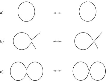
Fig. 1: Interaction vertices a) $U$, b) $V_{\propto}$ and c) $V_{\infty}$.

 

interaction point $\rho_{0}^{(j)}$ on the first sheet and then around $\bar{\rho}_{0}^{(j)}$ on the second sheet of the $\rho$ planes in Figs. 4 and 6.

A comment may be in order on the integration region for $\sigma_{0}$ in the closed intersection vertex $V_{\infty}$. At first sight it seems that the moduli parameter $\sigma_{0}$ should be integrated from 0 to $\pi$. However, since the configuration with $\pi/2\leq\sigma_{0}\leq\pi$ becomes the same as that with $0\leq\sigma_{0}\leq\pi/2$ if the twist operator $\mathchar 28938\relax$ is acted on either one of the two strings 1 or 2, we have an identity for the LPP vertex:

$$\langle v_{\infty}(1^{\mathrm{c}},2^{\mathrm{c}};\pi-\sigma_{0})|\mathchar 28938\relax^{(2)}\prod_{r=1^{\mathrm{c}},2^{\mathrm{c}}}{\cal P}^{(r)} = -\langle v_{\infty}(1^{\mathrm{c}},2^{\mathrm{c}};\sigma_{0})|\prod_{r=1^{\mathrm{c}},2^{\mathrm{c}}}{\cal P}^{(r)}$$ (3.19)

$$\hskip 50.00008pt(0\leq\sigma_{0}\leq\pi/2).$$

But there is an unoriented projection $\mathchar 28933\relax$ acting on the vertex and $\mathchar 28938\relax\mathchar 28933\relax=\mathchar 28933\relax$, the contribution of the configurations with $\pi/2\leq\sigma_{0}\leq\pi$ is actually the same as that with $\pi/2\leq\sigma_{0}\leq\pi$ in our final vertex. So we have restricted the integration region to $0\leq\sigma_{0}\leq\pi/2$ to correctly cover the moduli space only once. [The minus sign in Eq. (3.19) is important here and later. It should appear here since otherwise the integral $\int d\sigma_{0}\langle v_{\infty}(1^{\mathrm{c}},2^{\mathrm{c}};\sigma_{0})|b_{\sigma_{0}}$, if extended over $0\leq\sigma_{0}\leq\pi$, would vanish because of the fact $b_{\sigma_{0}}=(d\rho_{0}/d\sigma_{0})b_{\rho_{0}}=-b_{\pi-\sigma_{0}}$. More directly, as we shall see below, the LPP vertex $\langle v_{\infty}(1^{\mathrm{c}},2^{\mathrm{c}};\sigma_{0})|$ contains two ghost factors at the two interaction points $\sigma=\pi\pm\sigma_{0}$ if rewritten in terms of the HIKKO representation. The multiplication order of these two is opposite between the two configurations with $\sigma_{0}$ and $\pi-\sigma_{0}$, which yields the minus sign in Eq. (3.19).]

4 Action

We shall see later that there appears a divergence owing to the tachyon at order $g^{2}$ and it is canceled by the shift of the zero intercept parameter in $L_{0}$. Taking this into account in advance, we define here tilded (or, ‘bare’) BRS charges by shifting the zero intercept parameters in the usual (‘renormalized’) BRS charges $Q_{\rm B}^{\mathrm{o}}$ and $Q_{\rm B}^{\mathrm{c}}$ for open and closed strings, respectively, as follows:

$${\tilde{Q}}_{\rm B}^{\mathrm{o}} = Q_{\rm B}^{\mathrm{o}}+\lambda_{\mathrm{o}}g^{2}c_{0},$$

$${\tilde{Q}}_{\rm B}^{\mathrm{c}} = Q_{\rm B}^{\mathrm{c}}+\lambda_{\mathrm{c}}g^{2}c_{0}^{+},$$ (4.1)

where $\lambda_{\mathrm{o}}g^{2}$ and $\lambda_{\mathrm{c}}g^{2}$ are the amounts of the zero intercept shift for open and closed strings, respectively, which will be determined later by the gauge invariance requirement.

We can now give the more precise form for the action Eq. (1.1) and the gauge transformation Eq. (1) using the bra-ket notation:

$$S = -\hbox{${1\over 2}$}\langle R^{\mathrm{o}}(2,1)|\left|\mathchar 28937\relax\right>_{1}{\tilde{Q}}_{\rm B}^{(2)}\mathchar 28933\relax^{(2)}\left|\mathchar 28937\relax\right>_{2}-\hbox{${1\over 2}$}\langle R^{\mathrm{c}}(2,1)|\left|\mathchar 28936\relax\right>_{1}{\tilde{Q}}_{\rm B}^{(2)}{b^{-}_{0}}^{(2)}(b_{0}^{-}{\cal P}\mathchar 28933\relax)^{(2)}$$ (4.2)

$$\qquad{}+x_{u}g\,\langle U(2,1)|\left|\mathchar 28936\relax\right>_{1}\left|\mathchar 28937\relax\right>_{2}+x_{\propto}\,\hbox{${1\over 2}$}{g^{2}}\langle V_{\propto}(2,1)|\left|\mathchar 28937\relax\right>_{1}\left|\mathchar 28937\relax\right>_{2}$$

$$\qquad\qquad{}+x_{\infty}\,\hbox{${1\over 2}$}{g^{2}}\langle V_{\infty}(2,1)|\left|\mathchar 28936\relax\right>_{1}\left|\mathchar 28936\relax\right>_{2},$$

$$\delta({b_{0}^{-}}^{(1)}\left|\mathchar 28936\relax\right>_{1}) = -{\tilde{Q}}_{\rm B}^{(1)}(b_{0}^{-}{\cal P}\mathchar 28933\relax)^{(1)}\left|\mathchar 28931\relax^{\mathrm{c}}\right>_{1}+x_{\infty}g^{2}\langle V_{\infty}(3,2)|\left|R^{\mathrm{c}}(1,2)\right>\left|\mathchar 28931\relax^{\mathrm{c}}\right>_{3},$$

$$\delta\left|\mathchar 28937\relax\right>_{1} = x_{u}g\langle U(2,1^{\mathrm{c}})|\left|R^{\mathrm{o}}(1,2)\right>\left|\mathchar 28931\relax^{\mathrm{c}}\right>_{1^{\mathrm{c}}}.$$ (4.3)

where $(b_{0}^{-}{\cal P}\mathchar 28933\relax)^{(r)}$ is a shorthand notation for ${b_{0}^{-}}^{(r)}{\cal P}^{(r)}\mathchar 28933\relax^{(r)}$. Since the gauge transformation $\delta$ is the usual derivation, the gauge transformation parameter $\left|\mathchar 28931\relax^{\mathrm{c}}\right>$ is Grassmann even. The change of the action under this gauge transformation is given by

$$\delta S=\delta S_{1}+\delta S_{2}+\delta S_{3}+\delta S_{4},$$

$$\delta S_{1}=x_{u}g\langle U(1,1^{\mathrm{c}})|({\tilde{Q}}_{\rm B}^{(1)}+{\tilde{Q}}_{\rm B}^{(1^{\mathrm{c}})})\left|\mathchar 28937\relax\right>_{1}\left|\mathchar 28931\relax^{\mathrm{c}}\right>_{1^{\mathrm{c}}}$$

$$\delta S_{2}=+g^{2}\left[x_{u}^{2}\langle U(1,1^{\mathrm{c}})|\langle U(2,2^{\mathrm{c}})|\left|R^{\mathrm{o}}(1,2)\right>\right.$$

$$\hskip 55.00008pt-x_{\infty}\langle V_{\infty}(2^{\mathrm{c}},1^{\mathrm{c}})|({\tilde{Q}}_{\rm B}^{(1^{\mathrm{c}})}+{\tilde{Q}}_{\rm B}^{(2^{\mathrm{c}})})$$

$$\hskip 55.00008pt\left.+\lambda_{\mathrm{c}}\langle R^{\mathrm{c}}(2^{\mathrm{c}},1^{\mathrm{c}})|\{Q_{\rm B}^{(1^{\mathrm{c}})},\,{c_{0}^{+}}^{(1^{\mathrm{c}})}\}{b_{0}^{-}}^{(1^{\mathrm{c}})}\right]\left|\mathchar 28936\relax\right>_{1^{\mathrm{c}}}\left|\mathchar 28931\relax^{\mathrm{c}}\right>_{2^{\mathrm{c}}}$$

$$\delta S_{3}=+x_{u}g^{3}\left[-x_{\infty}\langle\check{U}(1,2^{\mathrm{c}})|\langle V_{\infty}(3^{\mathrm{c}},1^{\mathrm{c}})|\left|R^{\mathrm{c}}(2^{\mathrm{c}},3^{\mathrm{c}})\right>\right.$$

$$\hskip 70.0001pt+x_{\propto}\langle V_{\propto}(1,2)|\langle U(3,1^{\mathrm{c}})|\left|R^{\mathrm{o}}(2,3)\right>{\hbox{$\left]\vbox to0.0pt{}\right.\n@space$}}\left|\mathchar 28937\relax\right>_{1}\left|\mathchar 28931\relax^{\mathrm{c}}\right>_{1^{\mathrm{c}}}$$

$$\delta S_{4}=-x_{\infty}^{2}g^{4}\langle\check{V}_{\infty}(1^{\mathrm{c}},3^{\mathrm{c}})|\langle V_{\infty}(4^{\mathrm{c}},2^{\mathrm{c}})|\left|R^{\mathrm{c}}(3^{\mathrm{c}},4^{\mathrm{c}})\right>\left|\mathchar 28936\relax\right>_{1^{\mathrm{c}}}\left|\mathchar 28931\relax^{\mathrm{c}}\right>_{2^{\mathrm{c}}}.$$ (4.4)

Here the checked vertices $\langle\check{U}|$ and $\langle\check{V}_{\infty}|$ are those with a factor $b_{0}^{-}$ removed:

$$\langle U(1,2^{\mathrm{c}})|=\langle\check{U}(1,2^{\mathrm{c}})|{b_{0}^{-}}^{(2^{\mathrm{c}})},\hskip 20.00003pt\langle V_{\infty}(1,2)|=\langle\check{V}_{\infty}(1,2)|{b_{0}^{-}}^{(2)}.$$ (4.5)

In this calculation, it is useful to remember the symmetry properties $\langle V_{\propto}(1,2)|=\langle V_{\propto}(2,1)|$ and $\langle V_{\infty}(1,2)|=-\langle V_{\infty}(2,1)|$, and also the following Grassmann even-odd properties of the vertices: the open-closed transition vertex $\langle U|$ and open reflector $\langle R^{{\mathrm{o}}}|$ are odd and all the others $\langle R^{{\mathrm{c}}}|,\ \langle V_{\propto}|,\ \langle V_{\infty}|$ are even. These properties can easily be seen from the form of each term in the action (which is even, of course) and the fact that $\left|\mathchar 28937\relax\right>$ is even and $\left|\mathchar 28936\relax\right>$ odd.

5 Gauge invariance

In this section, we show that the parameters $\lambda_{\mathrm{c}},\lambda_{\mathrm{o}},x_{u},x_{\propto}$ and $x_{\infty}$ in the action (4.2) should satisfy

$$\lambda_{\mathrm{c}}=2\lambda_{\mathrm{o}}=-\lim_{a\rightarrow\infty}{2nx_{u}^{2}\over a^{2}},$$

$$x_{\infty}=nx_{u}^{2},$$

$$x_{\infty}=-4\pi ix_{\propto},$$ (5.1)

in order for the theory to be gauge invariant. To show this, let us now examine each term in Eq. (4) order by order.

5.1 Order $g$ invariance

It follows from the definition of the LPP vertex that

$$\langle U(1,1^{\mathrm{c}})|(Q_{\rm B}^{(1)}+Q_{\rm B}^{(1^{\mathrm{c}})})=0,$$ (5.2)

which has been proven first in Ref. ?, ?. This finishes the proof of order $g$ invariance. But the first term $\delta S_{1}$ in Eq. (4) contains also the order $g^{3}$ terms coming from the shift of the zero intercept parameter. They have to cancel out by themselves since no other counterparts appear to cancel them. So we here consider the condition for them to cancel, although they are of order $g^{3}$.

From the connection equation Eq. (3.3) for $\phi=c$, we have

$$\langle U(1,1^{\mathrm{c}})|\bigl{[}c^{(1^{\mathrm{c}})}(\sigma)+2c^{(1)}(\pi-\frac{\sigma}{2})\bigr{]}=0,$$

$$\langle U(1,1^{\mathrm{c}})|\bigl{[}\bar{c}^{(1^{\mathrm{c}})}(-\sigma)+2c^{(1)}(\pi+\frac{\sigma}{2})\bigr{]}=0.$$ (5.3)

Summing these two and performing integration $\int_{0}^{2\pi}d\sigma/2\pi$, we find

$$\langle U(1,1^{\mathrm{c}})|\bigl{[}{c_{0}}^{(1^{\mathrm{c}})}+{\bar{c}_{0}}^{(1^{\mathrm{c}})}+4{c_{0}}^{(1)}\bigr{]}=\langle U(1,1^{\mathrm{c}})|\ 2\bigl{[}{c_{0}^{+}}^{(1^{\mathrm{c}})}+2{c_{0}}^{(1)}\bigr{]}=0$$ (5.4)

Therefore, if we take

$$\lambda_{\mathrm{c}}=2\lambda_{\mathrm{o}},$$ (5.5)

it follows that

$$\langle U(1,1^{\mathrm{c}})|({\tilde{Q}}_{\rm B}^{(1)}+{\tilde{Q}}_{\rm B}^{(1^{\mathrm{c}})})=0.$$ (5.6)

The requirement (5.5) is natural since the zeroth order zero intercepts $\alpha_{0}^{\mathrm{o}}$ and $\alpha_{0}^{\mathrm{c}}$ for open and closed strings also satisfy the relation $\alpha_{0}^{\mathrm{c}}=2\alpha_{0}^{\mathrm{o}}=2$. Hereafter, we accept the relation of Eq. (5.5) and then the ‘order $g$’ gauge invariance $\delta S_{1}=0$ is realized.

5.2 Order $g^{2}$ invariance

In the order $g^{2}$ terms $\delta S_{2}$ in Eq. (4), the first $UU$ and the second $V_{\infty}$ terms are divergent for these correspond to singular configurations in moduli space, so that we need regularization for their evaluation. First, we rewrite the first terms as follows,

$$\langle U(1,1^{\mathrm{c}})|\langle U(2,2^{\mathrm{c}})|\left|R^{\mathrm{o}}(1,2)\right> = \lim_{T\rightarrow 0}\langle u(1,1^{\mathrm{c}})|\langle u(2,2^{\mathrm{c}})|e^{-(1/2)L_{0}^{(2)}T}\left|R^{\mathrm{o}}(1,2)\right>$$ (5.7)

$$\qquad{}\times e^{+(L^{(1^{\mathrm{c}})}+L^{(2^{\mathrm{c}})})T/2}\!\!\prod_{r=1^{\mathrm{c}},2^{\mathrm{c}}}\!\!(b_{0}^{-}{\cal P}\mathchar 28933\relax)^{(r)},$$

where $L\equiv L_{0}+\bar{L}_{0}$ for closed string. Here the unoriented projection operators for the intermediate open strings 1 and 2 have been dropped since $\langle u(1,1^{\mathrm{c}})|\mathchar 28933\relax^{(1)}{\cal P}^{(1^{\mathrm{c}})}=\langle u(1,1^{\mathrm{c}})|\mathchar 28933\relax^{(1^{\mathrm{c}})}{\cal P}^{(1^{\mathrm{c}})}$. $T$ is introduced as a regularization parameter and has the meaning of propagation time of the intermediate open string. The factor 1/2 in $e^{-(1/2)L_{0}^{(2)}T}$ is the factor $1/\alpha_{2}$ of the string length parameter $\alpha_{2}=2$ for the intermediate open string 2. We can replace the operator $e^{-(1/2)L_{0}^{(2)}T}$ by a more symmetric one $e^{-(L_{0}^{(1)}+L_{0}^{(2)})T/4}$ if necessary since $L_{0}^{(1)}=L_{0}^{(2)}$ in front of the reflector $\left|R^{\mathrm{o}}(1,2)\right>$. Note that we also have added the operator $e^{+(L^{(1^{\mathrm{c}})}+L^{(2^{\mathrm{c}})})T/2}$: this is because it almost cancels $e^{-(1/2)L_{0}^{(2)}T}=e^{-(L_{0}^{(1)}+L_{0}^{(2)})T/4}$ even for finite $T$ since the energy momentum tensor $T(\rho)$ is continuous on the vertices $\langle u(r,r^{\mathrm{c}})|$ aside from the interaction point, although the right hand side in Eq. (5.7), in any case, reduces to the left hand side as $T\rightarrow 0$, formally. The part $\langle u(1,1^{\mathrm{c}})|\langle u(2,2^{\mathrm{c}})|e^{-(1/2)L_{0}^{(2)}T}\left|R^{\mathrm{o}}(1,2)\right>$ can be evaluated according to the LPP’s “Generalized gluing and resmoothing” (GGR) theorem,[16] and so we obtain

$$\langle U(1,1^{\mathrm{c}})|\langle U(2,2^{\mathrm{c}})|\left|R^{\mathrm{o}}(1,2)\right>$$

$$\qquad{}=n\,\lim_{T\rightarrow 0}\langle v_{D_{2}}(1^{\mathrm{c}},2^{\mathrm{c}};T)|e^{+(L^{(1^{\mathrm{c}})}+L^{(2^{\mathrm{c}})})T/2}\!\!\!\prod_{r=1^{\mathrm{c}},2^{\mathrm{c}}}\!\!(b_{0}^{-}{\cal P}\mathchar 28933\relax)^{(r)},$$ (5.8)

where $\langle v_{D_{2}}(T)|$ is the LPP vertex, which we call D2 vertex, corresponding to the $\rho$ plane represented in Fig. 8, and the factor $n$ came from the trace of Chan-Paton factor of the intermediate open string.

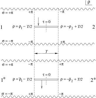
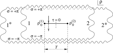
Fig. 8: The $\rho$ plane for the vertex $\langle v_{D_{2}}|$.

The second term in the order $g^{2}$ terms $\delta S_{2}$ in Eq. (4) is rewritten as

$$\langle V_{\infty}(1^{\mathrm{c}},2^{\mathrm{c}})|({\tilde{Q}}_{\rm B}^{(1^{\mathrm{c}})}+{\tilde{Q}}_{\rm B}^{(2^{\mathrm{c}})})=\int^{\frac{\pi}{2}}_{0}d\sigma_{0}\langle v_{\infty}(1^{\mathrm{c}},2^{\mathrm{c}};\sigma_{0})|\{Q_{\rm B},\,b_{\sigma_{0}}\}\prod_{r=1^{\mathrm{c}},2^{\mathrm{c}}}(b_{0}^{-}{\cal P}\mathchar 28933\relax)^{(r)}$$

$$\hskip 40.00006pt{}+\lambda_{\mathrm{c}}\int^{\frac{\pi}{2}}_{0}d\sigma_{0}\langle v_{\infty}(1^{\mathrm{c}},2^{\mathrm{c}};\sigma_{0})|b_{\sigma_{0}}({c_{0}^{+}}^{(1^{\mathrm{c}})}+{c_{0}^{+}}^{(2^{\mathrm{c}})})\prod_{r=1^{\mathrm{c}},2^{\mathrm{c}}}(b_{0}^{-}{\cal P}\mathchar 28933\relax)^{(r)}.$$ (5.9)

We now use the identity,[25, 30, 27]

$$\langle v_{\infty}(1^{\mathrm{c}},2^{\mathrm{c}};\sigma_{0})|\{Q_{\rm B},\,b_{\sigma_{0}}\} = \langle v_{\infty}(1^{\mathrm{c}},2^{\mathrm{c}};\sigma_{0})|T_{\sigma_{0}}$$ (5.10)

$$= {d\over d\sigma_{0}}\bigl{\{}\langle v_{\infty}(1^{\mathrm{c}},2^{\mathrm{c}};\sigma_{0})|\bigr{\}},$$

which follows from the fact that

$$T_{\sigma_{0}}=\{Q_{\rm B},\,b_{\sigma_{0}}\}=\left[\left({d\rho_{0}^{(1)}\over d\sigma_{0}}\right)\oint_{C_{1}}+\left({d\rho_{0}^{(2)}\over d\sigma_{0}}\right)\oint_{C_{2}}\right]\frac{d\rho}{2\pi i}T(\rho),$$ (5.11)

is the generator for the change of the moduli parameter $\sigma_{0}$ (since, generally, the contour integration of energy momentum tensor $\oint_{C_{Z}}(dz/2\pi i)T(z)$ along a closed path $C_{Z}$ encircling the point $Z$ is known[26] to give a generator for $\partial/\partial Z$). Then, the integral over $\sigma_{0}$ in the first term leaves only the surface terms:

$$\langle V_{\infty}(1^{\mathrm{c}},2^{\mathrm{c}})|({\tilde{Q}}_{\rm B}^{(1^{\mathrm{c}})}+{\tilde{Q}}_{\rm B}^{(2^{\mathrm{c}})}) = -\lim_{\sigma_{0}\rightarrow 0}\langle v_{\infty}(1^{\mathrm{c}},2^{\mathrm{c}};\sigma_{0})|\prod_{r=1^{\mathrm{c}},2^{\mathrm{c}}}(b_{0}^{-}{\cal P}\mathchar 28933\relax)^{(r)}$$ (5.12)

$${}+\lambda_{\mathrm{c}}\int^{\frac{\pi}{2}}_{0}d\sigma_{0}\langle v_{\infty}(1^{\mathrm{c}},2^{\mathrm{c}};\sigma_{0})|b_{\rho_{0}}({c_{0}^{+}}^{(1^{\mathrm{c}})}\!+{c_{0}^{+}}^{(2^{\mathrm{c}})})\!\!\prod_{r=1^{\mathrm{c}},2^{\mathrm{c}}}\!\!(b_{0}^{-}{\cal P}\mathchar 28933\relax)^{(r)},$$

where the surface term at the other end point $\sigma_{0}=\pi/2$ has dropped out since it vanishes by itself owing to the identity Eq. (3.19). We call this vertex $\langle v_{\infty}(\sigma_{0})|$ P2 vertex for short.

Fig. 7: The contours $C_{j}$ in Eq. (3.18).

 

The quantities Eq. (5.2) for D2 vertex and the first term of Eq. (5.12) for P2 vertex correspond to a common configuration as depicted in the Fig. 5.2 in the limit $T,\sigma_{0}\rightarrow 0$, and so have the well-known singularities owing to the tachyon and dilaton contributions. We want to evaluate this singularity in Eqs. (5.2) and (5.12) explicitly. For that purpose, it is convenient to map the $\rho$ plane to the whole complex $z$ plane. This map is constructed as follows: first, consider the former D2 case, corresponding to the diagram Fig. 8 with open string propagating as an intermediate state. By the usual Mandelstam mapping,

$$\rho=\ln(2-\zeta)-\ln(\zeta+2),$$ (5.13)

we can first map the $\rho$ plane of Fig. 8 to the Riemann surface, $\zeta$ plane. The cut between $\rho_{0}^{(1)}=-T/2$ and $\rho_{0}^{(2)}=T/2$ on the $\rho$ plane, which corresponds to the open string boundary, is mapped to the cut between $\zeta=-2a$ and $\zeta=2a$ on $\zeta$ plane:

$${T\over 2}=\ln{1+a\over 1-a}\ \Rightarrow\ a=\tanh{T\over 4}.$$ (5.14)

So $a$ is a real positive number in $0\leq a\leq 1$, corresponding the moduli $0\leq T\leq\infty$. This $\zeta$ plane, having two sheets as $\rho$ plane, is then mapped to the whole complex $z$ plane by the Joukowski transformation:

$$\zeta=z+\frac{a^{2}}{z}.$$ (5.15)

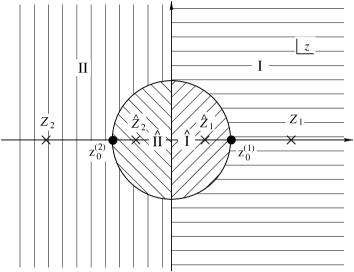
Fig. 10: The $z$ plane of the D2 vertex. Regions I and II ($\,\hat{\rm I}$ and $\hat{\rm II}\,$) correspond to the $\tau{<}0$ and $\tau{>}0$ regions on the first (second) sheet of the $\rho$ plane in Fig. 8, respectively.

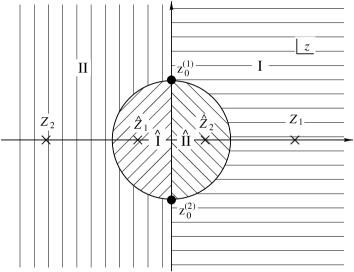
Fig. 11: The $z$ plane of the P2 vertex. Regions I and II  ($\,\hat{\rm I}$ and $\hat{\rm II}\,$) correspond to the regions 1 and 2 ($\,1^{*}$ and $2^{*}\,$) on the first (second) sheet of the $\rho$ plane in Fig. 6.

The correspondence between the each string domain of the $\rho$ plane and the $z$ plane is represented in Fig. 11. Note that the $z$ plane is now of a single sheet. The first sheet of $\rho$ (or $\zeta$) plane is mapped to the outer region of the circle with radius $|z|=a$ and the second sheet to the inner region. If $z$ is a root of Eq. (5.15) for a given $\zeta$ (or $\rho$), so is $a^{2}/z$. When a point $\rho$ on the first sheet is mapped to $z$ in the outer region, $|z|\geq a$, $\bar{\rho}$ on the second sheet corresponds to $a^{2}/{\bar{z}}$ in the inner region. Therefore, in particular, we have the following correspondence for the real string coordinate:

$$X^{\mu(1)}(\sigma_{1},\tau_{1})=\hbox{${1\over 2}$}{\hbox{$\left(\vbox to0.0pt{}\right.\n@space$}}X^{\mu(1)}(\rho)+\bar{X}^{\mu(1)}(\bar{\rho}){\hbox{$\left)\vbox to0.0pt{}\right.\n@space$}}\quad\Leftrightarrow\quad\hbox{${1\over 2}$}{\hbox{$\left(\vbox to0.0pt{}\right.\n@space$}}X^{\mu}(z)+X^{\mu}({a^{2}\over{\bar{z}}}){\hbox{$\left)\vbox to0.0pt{}\right.\n@space$}}.$$ (5.16)

Consider next the $\rho$ plane of Fig. 6, for the P2 vertex $V_{\infty}$. We should notice that this plane differs from the previous $\rho$ plane of Fig. 8, only by the cut structure which in this case corresponds to a cross cap instead of a open string boundary, and it is well-known that the mapping $\rho$ to $z$ in this case is given by the same one as above simply by changing the moduli from real $a$ to imaginary $ia$. The resultant $z$ plane is depicted in Fig. 11.

Therefore the evaluation of Eq. (5.2) and the first term of Eq. (5.12) can be carried out in a unified manner. The $\rho$ planes are mapped to the $z$ planes by the mapping

$$\rho=\ln\left(2-\bigl{(}z+\frac{q^{2}}{z}\bigr{)}\right)-\ln\left(z+\frac{q^{2}}{z}+2\right),$$ (5.17)

with real $q=a$ or imaginary $q=ia$ for D2 and P2 vertex cases, respectively. It is important for later consideration that on the $z$ plane in Fig. 11 or in 11, only one complex $z$ plane is needed for our analysis, and all of the insertion points of strings are on the real axis, the situation which is very similar to purely open strings system.

The interaction points are given by

$$\frac{d\rho}{dz}=0\ \ \ \Rightarrow\ \ \ z_{0}^{(1)}=+q,\ z_{0}^{(2)}=-q.$$ (5.18)

The point corresponding to the insertion of string fields are given by

$$Z_{1}=1+\sqrt{1-q^{2}},\hskip 20.00003pt\hat{Z}_{1}=1-\sqrt{1-q^{2}},$$ (5.19)

$$Z_{2}=-1-\sqrt{1-q^{2}},\hskip 20.00003pt\hat{Z}_{2}=-1+\sqrt{1-q^{2}}.$$ (5.20)

To discuss the singularity of the D2 and P2 vertices, it is convenient to use the HIKKO’s OSp symmetric expression for the vertex. In the Appendix A, we show the following expression for the LPP vertex a la HIKKO:

$$\langle v(1^{\mathrm{c}},2^{\mathrm{c}};q)|=N(q)\,{\textstyle{\atop 2^{\mathrm{c}}}}\!\langle\tilde{1},\tilde{1}|{\textstyle{\atop 1^{\mathrm{c}}}}\!\langle\tilde{1},\tilde{1}|\bigl{(}\sum_{r}\frac{b_{0}^{(r)}}{\alpha_{r}}\bigr{)}\exp(E_{\mathrm{H}}(1^{\mathrm{c}},2^{\mathrm{c}}))\,c(\rho_{0}^{(1)})c(\rho_{0}^{(2)}).$$ (5.21)

where the normalization factor $N(q)$ is given explicitly in Eq. (A.43) and the exponent $E_{\mathrm{H}}$ is the HIKKO’s OSP invariant quadratic operator given by[18, 19]

$$E_{\mathrm{H}}=\!\!\sum_{\stackrel{{\scriptstyle\scriptstyle m,n\geq 0}}{{\ \ \ r,s=1,\bar{1},2,\bar{2}}}}\!\!\!\!\bar{N}^{rs}_{mn}\left(\hbox{${1\over 2}$}{\alpha_{m}^{\mu}}^{(r)}\eta_{\mu\nu}{\alpha_{n}^{\nu}}^{(s)}+i\,{\gamma_{m}}^{(r)}{\beta_{n}}^{(s)}\right)\equiv\sum\bar{N}^{rs}_{mn}\hbox{${1\over 2}$}a_{m}^{(r)}\cdot a_{n}^{(s)},$$

$${\gamma_{n}}^{(r)}=i\,n\alpha_{r}{c_{n}}^{(r)},\qquad{\beta_{n}}^{(r)}={b_{n}}^{(r)}/{\alpha_{r}},$$ (5.22)

with the Fourier coefficients $\bar{N}^{rs}_{mn}$ of the Neumann function for the $X^{\mu}$ operators. Here we have used the following notation for OSp$(d,2|2)$ vector and invariant metric:

$$a_{m}^{M}=(\alpha_{m}^{\mu},\,\gamma_{m},\,\beta_{m}),$$

$$a\cdot b=a^{M}\eta_{MN}\,b^{N},\hskip 20.00003pt\eta_{MN}=\pmatrix{\eta_{\mu\nu}&&\cr&0&i\cr&-i&0\cr}.$$ (5.23)

From Eqs. (5.17) and (5.18), we see that the two interaction points $\rho_{0}^{(1,2)}$ on the $\rho$ plane are related with the parameter $q$ as

$${\rho_{0}}^{(2)}=-{\rho_{0}}^{(1)}=\ln\left(\frac{1+q}{1-q}\right).$$ (5.24)

${\rho_{0}}^{(r)}$ is real if $q=a$ and purely imaginary if $q=ia$. For real $q=a$ (D2 vertex), the interaction points $\rho_{0}^{(1,2)}$ are on the open string boundary as in Fig. 8, so that the holomorphic and anti-holomorphic parts are equal to each other. Then we find

$$c(\rho_{0}^{(1)}) = c^{(1)}({\rho_{0}}^{(1)}-T/2)=\hbox{${1\over 2}$}\left(c^{(1)}(0)+\bar{c}^{(1)}(0)\right)=C^{(1)}(0),$$

$$c(\rho_{0}^{(2)}) = -c^{(2)}(-{\rho_{0}}^{(2)}+T/2)=-\hbox{${1\over 2}$}\left(c^{(2)}(0)+\bar{c}^{(2)}(0)\right)=-C^{(2)}(0),$$ (5.25)

where we have defined

$$C(\rho)\equiv\hbox{${1\over 2}$}\bigl{(}c(\rho)+\bar{c}(\rho)\bigr{)}.$$ (5.26)

(Note that the argument of $\bar{c}$ is not $\bar{\rho}$ but $\rho$ here.)  If $q=ia$ (imaginary), on the other hand, from the connection condition of Eq. (3.9), we have $c^{(1)}(i\sigma)=-{\bar{c}}^{(2)}(-i\sigma)=+{\bar{c}}^{(1)}(i\sigma)$ at both interaction points $i\sigma=\rho_{0}^{(1)}=-i\sigma_{0}$ and $i\sigma=\rho_{0}^{(2)}=+i\sigma_{0}$, so that

$$c(\rho_{0}^{(1)}) = \hbox{${1\over 2}$}\left(c^{(1)}(-i{\sigma_{0}})+\bar{c}^{(1)}({-i\sigma_{0}})\right)=C^{(1)}(\rho_{0}^{(1)}),$$

$$c(\rho_{0}^{(2)}) = -\hbox{${1\over 2}$}\left(c^{(2)}(-i{\sigma_{0}})+\bar{c}^{(2)}(-{i\sigma_{0}})\right)=-C^{(2)}(\rho_{0}^{(1)}).$$ (5.27)

These ghost factors Eqs. (5.25) and Eq. (5.27) for D2 and P2 cases, respectively, look very different. We, however, note that, for the former D2 case, what should be evaluated is not the LPP vertex $\langle v_{D_{2}}(1^{\mathrm{c}},2^{\mathrm{c}};T)|$ itself but that multiplied by the operator $e^{+(L^{(1^{\mathrm{c}})}+L^{(2^{\mathrm{c}})})T/2}$, as seen in Eq. (5.2). So, using Eqs. (5.21) and (5.25), we have

$$\langle v(1^{\mathrm{c}},2^{\mathrm{c}};q=a)|e^{+(L^{(1^{\mathrm{c}})}+L^{(2^{\mathrm{c}})})T/2}$$

$$=N(q)\,{\textstyle{\atop 2^{\mathrm{c}}}}\!\langle\tilde{1},\tilde{1}|{\textstyle{\atop 1^{\mathrm{c}}}}\!\langle\tilde{1},\tilde{1}|\bigl{(}\sum_{r}\frac{b_{0}^{(r)}}{\alpha_{r}}\bigr{)}\exp(\hat{E}_{\mathrm{H}}(1^{\mathrm{c}},2^{\mathrm{c}}))\left(-\hat{C}^{(1)}(0)\hat{C}^{(2)}(0)\right),$$ (5.28)

with hatted operators denoting $\hat{\cal O}=e^{-(L^{(1^{\mathrm{c}})}+L^{(2^{\mathrm{c}})})T/2}{\cal O}e^{+(L^{(1^{\mathrm{c}})}+L^{(2^{\mathrm{c}})})T/2}$. This hat operation is equivalent to replacing all the oscillators by

$$(\hat{\alpha}_{n}^{\mu},\ \hat{c}_{n},\ \hat{b}_{n})=(e^{nT/2}\alpha_{n}^{\mu},\ e^{nT/2}c_{n},\ e^{nT/2}b_{n}).$$ (5.29)

So, now the ghost factors become

$$-\hat{C}^{(1)}(0)\hat{C}^{(2)}(0)=-C^{(1)}(-T/2)C^{(2)}(-T/2)=-C^{(1)}(\rho_{0}^{(1)})C^{(2)}(\rho_{0}^{(1)}),$$ (5.30)

since $\rho_{0}^{(1)}=-T/2$ in this D2 case. Therefore the ghost factor $c(\rho_{0}^{(1)})c(\rho_{0}^{(2)})$ in Eq. (5.21) can now be written as $-C^{(1)}(\rho_{0}^{(1)})C^{(2)}(\rho_{0}^{(1)})$ commonly for the D2 and P2 cases.

The exponent $\hat{E}_{\mathrm{H}}(1^{\mathrm{c}},2^{\mathrm{c}})$ for D2 case is given by the same expression as $E_{\mathrm{H}}(1^{\mathrm{c}},2^{\mathrm{c}})$ in Eq. (5.22) with the replacement Eq. (5.29) done for all the oscillators, while no such is done for the P2 case. But we shall see shortly that this also helps to make the expressions common for both cases.

Since we want to know the singular structure of the LPP vertex in the limit $T,\ \sigma_{0}\rightarrow 0$, we have only to know the behavior of the exponent $E_{\mathrm{H}}$ around $q\sim 0$, which is written in terms of the Neumann coefficients $\bar{N}^{rs}_{mn}$. We can do this task by expanding the Neumann function directly. The Neumann function on the $z$ plane is given by

$$N(z,z^{\prime}) = \ln\left|z-z^{\prime}\right|+\ln\left|1-\frac{q^{2}}{z\bar{z}^{\prime}}\right|$$ (5.32)

$$= \ln\left|z-z^{\prime}\right|-\ln\left|z-\bar{z}^{\prime}\right|+\ln\left|z+\frac{q^{2}}{z}-\bar{z}^{\prime}-\frac{q^{2}}{\bar{z}^{\prime}}\right|.$$

Since $\bar{N}^{rs}_{mn}$ appear as Fourier coefficients of the Neumann function Eq. (5.32), namely the coefficients of the terms $w_{r}^{n}w^{\prime\,m}_{s}=e^{n(\tau_{r}+i\sigma_{r})}e^{m(\tau^{\prime}_{s}+i\sigma^{\prime}_{s})}$, we rewrite it by substituting

$$z = \alpha_{r}W_{r}+\sqrt{W_{r}^{2}-q^{2}}=2\alpha_{r}\left(W_{r}-{q^{2}\over 4W_{r}}\right)+O(q^{4})$$ (5.33)

$${\rm with}\quad W_{r}\equiv{1-w_{r}\over 1+w_{r}},\quad\alpha_{1}=+1,\ \alpha_{2}=-1,$$

which follows from the mapping of Eq. (5.17) and the relation $\rho=\alpha_{r}\rho_{r}=\alpha_{r}\ln w_{r}$ in the string region $r=1$ and 2.

Actually, however, the last relation $\rho=\alpha_{r}\rho_{r}=\alpha_{r}\ln w_{r}$ applies only to the P2 vertex case, and the correct one for the D2 vertex case is $\rho=\alpha_{r}(\rho_{r}-T/2)=\alpha_{r}\ln(w_{r}e^{-T/2})$. So the variable $w_{r}$ in Eq. (5.33) should be understood as standing for $w_{r}e^{-T/2}$ for D2 case. This means that if we find the terms of the form $A^{rs}_{mn}w_{r}^{n}w^{\prime\,m}_{s}$ by writing the Neumann function in terms of the variable $w_{r}$ in Eq. (5.33), the true Neumann coefficients $\bar{N}^{rs}_{mn}$ in D2 case is given by $\bar{N}^{rs}_{mn}=A^{rs}_{mn}e^{-nT/2}e^{-mT/2}$. But recall that what we need for the D2 case is not the exponent $E_{\mathrm{H}}$ but $\hat{E}_{\mathrm{H}}$, for which, since the replacement Eq. (5.29) is done, the coefficients of the oscillators are given by $\bar{N}^{rs}_{mn}e^{nT/2}e^{mT/2}$ and just equal the coefficients $A^{rs}_{mn}$. So, for both D2 and P2 cases, we can unifiedly find the desired Neumann coefficients simply by using Eq. (5.33).

Now, substituting Eq. (5.33) into Eq. (5.32), we easily find

$$N(\rho_{r},\rho^{\prime}_{s}) = \ln\left|w_{r}-w^{\prime}_{s}\right|+{q^{2}\over 2}\sum_{m,n\geq 1}\left[(w_{r}^{m}-{\bar{w}}_{r}^{m})(w^{\prime\,n}_{s}-{\bar{w}}^{\prime\,n}_{s})\right]$$

$$\qquad\qquad+(\hbox{irrelevant terms})\qquad\hbox{for}\ \ (r,s)=(1,1),\,(2,2)$$

$$= -\sum_{n\geq 1}{1\over 2n}\left(w_{r}^{n}w^{\prime\,n}_{s}+{\bar{w}}_{r}^{n}{\bar{w}}^{\prime\,n}_{s}\right)-{q^{2}\over 2}\sum_{m,n\geq 1}\left[(w_{r}^{m}-{\bar{w}}_{r}^{m})(w^{\prime\,n}_{s}-{\bar{w}}^{\prime\,n}_{s})\right]$$

$$\qquad\qquad+(\hbox{irrelevant terms})\qquad\hbox{for}\ \ (r,s)=(1,2),\,(2,1).$$

The (irrelevant terms) stands for $2\ln 2-\ln\left|(1+w_{r})(1+w^{\prime}_{s})\right|$ which yields functions of a single variable $w_{r}$ or $w^{\prime}_{s}$, not contributing to the exponent $E_{\mathrm{H}}$ in the presence of the momentum conservation. The exponent $E_{\mathrm{H}}$ can now be obtained from this by formally performing replacements $(w_{r}^{m},\ {\bar{w}}_{r}^{m},\ w^{\prime\,n}_{s},\ {\bar{w}}^{\prime\,n}_{s})\rightarrow(a^{(r)}_{m},\ \bar{a}^{(r)}_{m},\ a^{(s)}_{n},\ \bar{a}^{(s)}_{n})$, discarding the free propagation term $\ln\left|w_{r}-w^{\prime}_{s}\right|$ as well as irrelevant terms:

$$E_{\mathrm{H}}(1^{\mathrm{c}},2^{\mathrm{c}}) = E^{\mathrm{c}}_{12}+\frac{q^{2}}{2}\sum_{m\geq 1}({a_{m}}^{(1)}-{\bar{a}_{m}}^{(1)})\cdot\sum_{n\geq 1}({a_{n}}^{(1)}-{\bar{a}_{n}}^{(1)})$$ (5.35)

$$+\frac{q^{2}}{2}\sum_{m\geq 1}({a_{m}}^{(2)}-{\bar{a}_{m}}^{(2)})\cdot\sum_{n\geq 1}({a_{n}}^{(2)}-{\bar{a}_{n}}^{(2)})$$

$$-q^{2}\sum_{m\geq 1}({a_{m}}^{(1)}-{\bar{a}_{m}}^{(1)})\cdot\sum_{n\geq 1}({a_{n}}^{(2)}-{\bar{a}_{n}}^{(2)})+O(q^{4}),$$

where $E^{\mathrm{c}}_{12}$ is the exponent of the closed reflector defined in Eq. (2), and we have used an OSp invariant notation $a_{m}^{M}=(\alpha_{m}^{\mu},\,\gamma_{m},\,\beta_{m})$ and $a\cdot b=a^{M}\eta_{MN}\,b^{N}$ introduced in Eq. (5.23). The appearance of the reflector is natural since the configurations of D2 and P2 vertices both reduce to a mere connection of two closed strings when $T,\ \sigma_{0}$ go to zero. Substitute this expanded from for $E_{\mathrm{H}}(1^{\mathrm{c}},2^{\mathrm{c}})$ (which is in fact $\hat{E}_{\mathrm{H}}(1^{\mathrm{c}},2^{\mathrm{c}})$ for D2 case) into Eq. (5.21) (or Eq. (5.28) for D2 case) and multiply ${b_{0}^{-}}^{(1)}{b_{0}^{-}}^{(2)}$ to it. Then, noting

$${\textstyle{\atop 2^{\mathrm{c}}}}\!\langle\tilde{1},\tilde{1}|{\textstyle{\atop 1^{\mathrm{c}}}}\!\langle\tilde{1},\tilde{1}|\bigl{(}\sum_{r}\frac{b_{0}^{(r)}}{\alpha_{r}}\bigr{)}{b_{0}^{-}}^{(1)}{b_{0}^{-}}^{(2)}$$

$$\qquad\quad=-{\textstyle{\atop 2^{\mathrm{c}}}}\!\langle 1,1|{\textstyle{\atop 1^{\mathrm{c}}}}\!\langle 1,1|(c_{0}^{+(1)}+c_{0}^{+(2)})(c_{0}^{-(1)}+c_{0}^{-(2)}){b_{0}^{-}}^{(1)}.$$ (5.36)

we find

$$\langle v(1^{\mathrm{c}},2^{\mathrm{c}};q)|{b_{0}^{-}}^{(1)}{b_{0}^{-}}^{(2)} = N(q)\,\langle R^{\mathrm{c}}(1^{\mathrm{c}},2^{\mathrm{c}})|C^{(1)}(\rho_{0}^{(1)})C^{(2)}(\rho_{0}^{(1)})$$ (5.37)

$$\hskip 30.00005pt\times\left\{1+q^{2}{\cal D}^{(1)}(0)+O(q^{4})\right\}{b_{0}^{-}}^{(1)},$$

where we have defined

$${\cal D}(\rho)=-:\Bigl{\{}\hbox{${1\over 2}$}\Bigl{(}\frac{dX}{d\rho}(\rho)-\frac{d\bar{X}}{d\bar{\rho}}(\bar{\rho})\!\Bigr{)}^{2}\!+\left({dc\over d\rho}(\rho)-{d{\bar{c}}\over d\bar{\rho}}(\bar{\rho})\right)\bigl{(}b(\rho)-\bar{b}(\bar{\rho})\bigr{)}\Bigr{\}}:\,.$$ (5.38)

Note that this ${\cal D}(0)$ is commutative with the ghost factor $C(\rho_{0}^{(1)})$ since $b(0)-\bar{b}(0)$ contained in the former anti-commutes with $C(\rho_{0}^{(1)})=\hbox{${1\over 2}$}\bigl{(}c(\rho_{0}^{(1)})+{\bar{c}}(\rho_{0}^{(1)})\bigr{)}$. [This explains why we have rewritten the original ghost factor $c(\rho_{0}^{(1)})$ into $C(\rho_{0}^{(1)})$ as done in in Eqs. (5.25) and Eq. (5.27). If we had kept using $c(\rho_{0}^{(1)})$, we would have encountered a divergent expression like $b(0)c(\rho_{0}^{(1)})\sim 1/\rho_{0}^{(1)}$ as $\rho_{0}^{(1)}\rightarrow 0$.] We replace $C^{(2)}(\rho_{0}^{(1)})$ by $-C^{(1)}(-\rho_{0}^{(1)})$ since they are equal on the reflector $\langle R^{\mathrm{c}}(1^{\mathrm{c}},2^{\mathrm{c}})|$, and expand the two ghost factors in powers of $q$ using Eq. (5.24):

$$C^{(1)}(-{\rho_{0}}^{(1)})C^{(1)}({\rho_{0}}^{(1)})=q\,C^{(1)}\frac{dC^{(1)}}{d\rho}(0)+q^{3}\,{\cal A}(0)+O(q^{5}),$$ (5.39)

where ${\cal A}$ is defined by

$${\cal A}(\rho)=\frac{1}{3}C\frac{dC}{d\rho}-2\frac{dC}{d\rho}\frac{d^{2}C}{d\rho^{2}}+\frac{2}{3}C\frac{d^{3}C}{d\rho^{3}}.$$ (5.40)

Finally, substituting Eqs. (A.43) and (5.39) to Eq. (5.37), we obtain

$$\langle v(1^{\mathrm{c}},2^{\mathrm{c}};q)|{b_{0}^{-}}^{(1)}{b_{0}^{-}}^{(2)}$$

$$\qquad\quad=\langle R^{\mathrm{c}}(1^{\mathrm{c}},2^{\mathrm{c}})|\left\{\frac{2}{q^{2}}C^{(1)}\frac{dC^{(1)}}{d\rho}(0)+{\cal B}^{(1)}(0)+O(q^{2})\right\}{b_{0}^{-}}^{(1)},$$ (5.41)

with

$${\cal B}(\rho)=\hbox{${1\over 2}$}\left({\cal A}-3C\frac{dC}{d\rho}+C\frac{dC}{d\rho}{\cal D}\right).$$ (5.42)

This Eq. (5.2) is a result which applies both to D2 and P2 vertices by putting $q=a$ and $q=ia$, respectively. In the limit $q\rightarrow 0$ (i.e., $T\rightarrow 0$ for D2 and $\sigma_{0}\rightarrow 0$ for P2 cases), this has two contributions: the first divergent term $\propto 1/q^{2}$ corresponds to the tachyon contribution and the second to the dilaton, as anticipated. The powers of $q$ in these are reduced by 1 since a power $q^{1}$ came from the product of two ghost factors $C^{(1)}(-{\rho_{0}}^{(1)})C^{(1)}({\rho_{0}}^{(1)})$ at the interaction points which vanish at the coincident limit.

At last, we can determine the relation for the parameters of $x_{u}$, $x_{\infty}$ and $\lambda_{c}$ to make the action gauge invariant. Since the result Eq. (5.2) is common to D2 and P2 vertices, the ${\cal B}^{(1)}(0)$ term can be canceled between the first two terms in $\delta S_{2}$ in Eq. (4), if we take $nx_{u}^{2}=x_{\infty}$:

$$x_{u}^{2}\langle U(1,1^{\mathrm{c}})|\langle U(2,2^{\mathrm{c}})|\left|R^{\mathrm{o}}(1,2)\right>+x_{\infty}\langle V_{\infty}(1^{\mathrm{c}},2^{\mathrm{c}})|({\tilde{Q}}_{\rm B}^{(1)}+{\tilde{Q}}_{\rm B}^{(2)})$$

$$=\lim_{a\rightarrow 0}\frac{4nx_{u}^{2}}{a^{2}}\langle R^{\mathrm{c}}(1^{\mathrm{c}},2^{\mathrm{c}})|C^{(1)}\frac{dC^{(1)}}{d\rho}(0)\,{b_{0}^{-}}^{(1)}\prod_{r=1^{\mathrm{c}},2^{\mathrm{c}}}({\cal P}\mathchar 28933\relax)^{(r)}$$

$$\ \ {}+x_{\infty}\lambda_{\mathrm{c}}\int^{\frac{\pi}{2}}_{0}d\sigma_{0}\langle v_{\infty}(1^{\mathrm{c}},2^{\mathrm{c}};\sigma_{0})|b_{\sigma_{0}}({c_{0}^{+}}^{(1^{\mathrm{c}})}\!{+}{c_{0}^{+}}^{(2^{\mathrm{c}})})\!\!\!\prod_{r=1^{\mathrm{c}},2^{\mathrm{c}}}\!\!(b_{0}^{-}{\cal P}\mathchar 28933\relax)^{(r)}\!,$$ (5.43)

where we have used $\langle V_{\infty}(2^{\mathrm{c}},1^{\mathrm{c}})|=-\langle V_{\infty}(1^{\mathrm{c}},2^{\mathrm{c}})|$, and note the minus sign in the first term in Eq. (5.12). The first singular term, due to the existence of the tachyon in bosonic strings, did not cancel but added up between the two since $q^{2}=a^{2}$ for D2 and $q^{2}=-a^{2}$ for P2. However, since it can be rewritten into the form of a BRS transform as

$$\langle R^{\mathrm{c}}(1^{\mathrm{c}},2^{\mathrm{c}})|C^{(1)}\frac{dC^{(1)}}{d\rho}(0)\,{b_{0}^{-}}^{(1)}{\cal P}^{(1)}{\cal P}^{(2)}$$

$$\qquad\quad=\langle R^{\mathrm{c}}(1^{\mathrm{c}},2^{\mathrm{c}})|\{Q_{\rm B}^{(1^{\mathrm{c}})},\,\hbox{${1\over 2}$}{c_{0}^{+}}^{(1^{\mathrm{c}})}\}\,{b_{0}^{-}}^{(1)}{\cal P}_{1}{\cal P}_{2},$$ (5.44)

it turns out that it can be canceled by the third term in $\delta S_{2}$ in Eq. (4) if we set

$$\lambda_{\mathrm{c}}=-\lim_{a\rightarrow 0}{2nx_{u}^{2}\over a^{2}}.$$ (5.45)

This corresponds to an infinite renormalization of the zero intercept parameter as mentioned before, and explains the reason why we have had to define the ‘bare’ BRS charge ${\tilde{Q}}_{\rm B}$ by shifting the zero intercept parameter.

Finally, let us show that the remaining second term in Eq. (5.43) also vanishes. First we note that

$$\langle v_{\infty}(1^{\mathrm{c}},2^{\mathrm{c}};\sigma_{0})|b_{\sigma_{0}} = \langle v_{\infty}(1^{\mathrm{c}},2^{\mathrm{c}};\sigma_{0})|\left(-i\oint_{C_{1}}+i\oint_{C_{2}}\right)\frac{d\rho}{2\pi i}b(\rho)$$ (5.46)

$$= \langle v_{\infty}(1^{\mathrm{c}},2^{\mathrm{c}};\sigma_{0})|\left(-i\oint_{C_{\hbox{$z$}_{0}^{\hbox{$(1)$}}}}+i\oint_{C_{\hbox{$z$}_{0}^{\hbox{$(2)$}}}}\right)\frac{dz}{2\pi i}\left({dz\over d\rho}\right)b(\rho)$$

$$= A(q)\langle v_{\infty}(1^{\mathrm{c}},2^{\mathrm{c}};\sigma_{0})|\bigl{(}b(z_{0}^{(1)})+b(z_{0}^{(2)})\bigr{)},$$

with $A(q)=iq(1-q^{2})/2$, where we have used Eq. (3.18) and $\rho_{0}^{(1)}=-\rho_{0}^{(2)}=-i\sigma_{0}$ for the definition of $b_{\sigma_{0}}$. The contour $C_{1}-C_{2}$ on the $\rho$ plane is deformed as drawn

Fig. 9: The configuration yielding the singularities in the D2 and P2 vertices.

 

in Fig. 7 a), and then mapped to $C_{\hbox{$z$}_{0}^{\hbox{$(1)$}}}-C_{\hbox{$z$}_{0}^{\hbox{$(2)$}}}$ on the $z$ plane where $C_{\hbox{$z$}_{0}^{\hbox{$(i)$}}}$ are closed contours encircling the interaction points $z_{0}^{(i)}$ in Fig. 11. Eqs. (A.17), (5.18) and (5.20) have been used for the evaluation of the contour integration on the $z$ plane. Next, the ghost zero-mode factor $({c_{0}^{+}}^{(1^{\mathrm{c}})}+{c_{0}^{+}}^{(2^{\mathrm{c}})})=\hbox{${1\over 2}$}({c_{0}}^{(1^{\mathrm{c}})}+{{\bar{c}}_{0}}^{(1^{\mathrm{c}})}+{c_{0}}^{(2^{\mathrm{c}})}+{{\bar{c}}_{0}}^{(2^{\mathrm{c}})})$ in the second term, which is first written as an integral over $\sigma$, can also be rewritten as an integral over $z$ again going to the $z$ plane. The integral contour can be deformed to the closed paths $C_{\hbox{$z$}_{0}^{\hbox{$(1)$}}}+C_{\hbox{$z$}_{0}^{\hbox{$(2)$}}}$ around the interaction points, and we find:

$$\langle v_{\infty}(1^{\mathrm{c}},2^{\mathrm{c}};\sigma_{0})|b_{\sigma_{0}}({c_{0}^{+}}^{(1^{\mathrm{c}})}+{c_{0}^{+}}^{(2^{\mathrm{c}})})$$

$$\ =\hbox{${1\over 2}$}A(q)\langle v_{\infty}(1^{\mathrm{c}},2^{\mathrm{c}};\sigma_{0})|\Bigl{(}\oint_{C_{\hbox{$z$}_{0}^{\hbox{$(1)$}}}}\!\!\!+\oint_{C_{\hbox{$z$}_{0}^{\hbox{$(2)$}}}}\Bigr{)}\frac{dz}{2\pi i}\left(\frac{d\rho}{dz}\right)^{2}\!\bigl{(}b(z_{0}^{(1)})\!+b(z_{0}^{(2)})\bigr{)}\,c(z).\hskip 30.00005pt$$ (5.47)

But, although $\langle{b(z_{0}^{(i)})c(z)}\rangle=1/(z_{0}^{(i)}-z)$, since the factor $(d\rho/dz)^{2}$ contains double zero $(z_{0}^{(i)}-z)^{2}$, the integrand is regular around the interaction points and the contour integral vanishes. Thus we have finished the proof of the O($g^{2}$) gauge invariance $\delta S_{2}=0$ and found the first two relations in Eq. (5.1) for the parameters.

5.3 Order $g^{3}$ and $g^{4}$ invariance

Now we turn to the consideration of the order $g^{3}$ terms $\delta S_{3}$ in Eq. (4). Again, inserting a propagator of the intermediate state, we rewrite the first term of the two $O(g^{3})$ terms into the form

$$\langle\check{U}(1,2^{\mathrm{c}})|\langle V_{\infty}(3^{\mathrm{c}},1^{\mathrm{c}})|\left|R^{\mathrm{c}}(2^{\mathrm{c}},3^{\mathrm{c}})\right>$$ (5.48)

$$= \lim_{\tau\rightarrow 0}\int_{0}^{\frac{\pi}{2}}\,d\sigma_{0}\int_{0}^{2\pi}\frac{d\theta}{2\pi}\langle u(1,2^{\mathrm{c}})|\langle v_{\infty}(3^{\mathrm{c}},1^{\mathrm{c}};\sigma_{0})|b_{\sigma_{0}}{b_{0}^{-}}^{(3^{\mathrm{c}})}$$

$$\hskip 80.00012pt\times e^{-\tau(L_{0}^{(3^{\mathrm{c}})}+\bar{L}_{0}^{(3^{\mathrm{c}})})}e^{i\theta(L_{0}^{(3^{\mathrm{c}})}-\bar{L}_{0}^{(3^{\mathrm{c}})})}\left|R^{\mathrm{c}}(2^{\mathrm{c}},3^{\mathrm{c}})\right>\left(b_{0}^{-}{\cal P}\mathchar 28933\relax\right)^{(1^{\mathrm{c}})}$$

$$= \lim_{\tau\rightarrow 0}\int_{0}^{\frac{\pi}{2}}\,d\sigma_{0}\int_{0}^{2\pi}\frac{d\theta}{2\pi}\langle v_{1}(1,1^{\mathrm{c}};\sigma_{0},\theta,\tau)|b_{\sigma_{0}}b_{C_{\theta}}\left(b_{0}^{-}{\cal P}\mathchar 28933\relax\right)^{(1^{\mathrm{c}})},$$

where $\tau$ is the propagation time interval, the explicit expression for ${\cal P}=\int_{0}^{2\pi}(d\theta/2\pi)\newline \exp(i\theta(L_{0}-\bar{L}_{0}))$ was inserted for ${\cal P}^{(3)}$, and $\langle v_{1}(\sigma_{0},\theta,\tau)|$ denotes the effective LPP vertex following from the GGR theorem, which corresponds to the string diagram depicted in Fig. 14. (We introduced $\tau$ for clarity for drawing the figure, although there occurs actually no singularity here even at $\tau=0$.)  $b_{C_{\theta}}\equiv(1/2)\oint_{C_{\theta}}d\rho/(2\pi i)\,b(\rho)$ is a rewriting of ${b_{0}^{-}}^{(3^{\mathrm{c}})}=(1/2)(b_{0}-{\bar{b}}_{0})^{(3^{\mathrm{c}})}$ and the contour $C_{\theta}$ is the path traversing the intermediate closed string as drawn in Fig. 14.

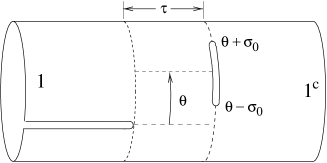
Fig. 13: The string diagram corresponding to the vertex $\langle v_{1}(\sigma_{0},\theta,\tau)|$.

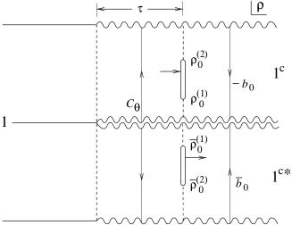
Fig. 14: The $\rho$ plane of the vertex $\langle v_{1}(\sigma_{0},\theta,\tau)|$.

Since ${b_{0}^{-}}^{(1^{\mathrm{c}})}$ factor for the external closed string $1^{\mathrm{c}}$ is also multiplied in Eq. (5.48), we can replace $b_{C_{\theta}}$ by $b_{C_{\theta}}-{b_{0}^{-}}^{(1^{\mathrm{c}})}$, and the latter can be seen to reduce to the following expression by making a deformation of the integration contour as drawn in Fig. 7 b):

$$b_{C_{\theta}}-{b_{0}^{-}}^{(1^{\mathrm{c}})}=-\hbox{${1\over 2}$}\left(\oint_{C_{1}}+\oint_{C_{2}}\right)\frac{d\rho}{2\pi i}b(\rho)=-\hbox{${1\over 2}$}(b_{\rho_{0}^{(1)}}+b_{\rho_{0}^{(2)}}),$$ (5.49)

where $C_{i}$ ($i=1,2$) are the closed contours given before in Fig. 5.2. This expression can also be understood from the meaning of $b_{C_{\theta}}$: it is originally the anti-ghost factor $b_{0}^{-(3)}$ corresponding to the quasi-conformal deformation for the change of $\theta$, whereas the $\theta$ change is now equivalent to shifting the interaction points $\rho_{0}^{(1)}=\tau_{0}+i(\theta-\sigma_{0})$ and $\rho_{0}^{(2)}=\tau_{0}+i(\theta+\sigma_{0})$ simultaneously by a common amount, and $b_{\rho_{0}^{(i)}}$ are clearly the anti-ghost factors corresponding to the shift of $\rho_{0}^{(i)}$.

On the other hand, the other anti-ghost factor $b_{\sigma_{0}}$ is

$$b_{\sigma_{0}}=-i(b_{\rho_{0}^{(1)}}-b_{\rho_{0}^{(2)}})$$ (5.50)

by the definition Eq. (3.18). Substituting this and Eq. (5.49) into Eq. (5.48), we find

$$\langle\check{U}(1,2^{\mathrm{c}})|\langle V_{\infty}(3^{\mathrm{c}},1^{\mathrm{c}})|\left|R^{\mathrm{c}}(2^{\mathrm{c}},3^{\mathrm{c}})\right>$$

$$\qquad{}=i\lim_{\tau\rightarrow 0}\int_{0}^{\frac{\pi}{2}}\,d\sigma_{0}\int_{0}^{2\pi}\frac{d\theta}{2\pi}\langle v_{1}(1,1^{\mathrm{c}};\sigma_{0},\theta,\tau)|b_{\rho_{0}^{(1)}}b_{\rho_{0}^{(2)}}(b_{0}^{-}{\cal P}\mathchar 28933\relax)^{1^{\mathrm{c}}}.$$ (5.51)

The second one of the two $O(g^{3})$ terms $\delta S_{3}$ in Eq. (4) is rewritten as

$$\langle V_{\propto}(1,2)|\langle U(3,1^{\mathrm{c}})|\left|R^{\mathrm{o}}(2,3)\right>$$ (5.52)

$$= -\lim_{\tau\rightarrow 0}\int_{0\leq\sigma_{1}\leq\sigma_{2}\leq\pi}d\sigma_{1}d\sigma_{2}\langle v_{\propto}(1,2;\sigma_{1},\sigma_{2})|\langle u(3,1^{\mathrm{c}})|b_{\sigma_{1}}b_{\sigma_{2}}e^{-\tau L_{0}^{(3)}}\left|R^{\mathrm{o}}(2,3)\right>\left(b_{0}^{-}{\cal P}\mathchar 28933\relax\right)^{(1^{\mathrm{c}})}$$

$$= +4\lim_{\tau\rightarrow 0}\int_{0\leq\sigma_{1}\leq\sigma_{2}\leq\pi}d\sigma_{1}d\sigma_{2}\langle v_{2}(1,1^{\mathrm{c}};\sigma_{1},\sigma_{2},\tau)|b_{\rho_{0}^{(1)}}b_{\rho_{0}^{(2)}}\left(b_{0}^{-}{\cal P}\mathchar 28933\relax\right)^{(1^{\mathrm{c}})},$$

where the minus in front comes from the order exchange of $b_{0}^{-(1^{\mathrm{c}})}$ and $\left|R^{\mathrm{o}}(2,3)\right>$, and the factor $-4$ from $b_{\sigma_{i}}=(d\rho_{0}^{(i)}/d\sigma_{i})b_{\rho_{0}^{(i)}}=2ib_{\rho_{0}^{(i)}}$ since $\rho_{0}^{(i)}=\alpha_{1}(\tau_{0}+i\sigma_{i})$ and $\alpha_{1}=2$ (Note that the interaction points are now on the open string side). $\langle v_{2}(\sigma_{1},\sigma_{2},\tau)|$ represents the effective LPP vertex corresponding to the string diagram depicted in Fig.16,

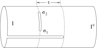
Fig. 15: The string diagram corresponding to the vertex $\langle v_{2}(\sigma_{1},\sigma_{2},\tau)|$.

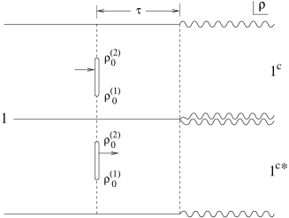
Fig. 16: The $\rho$ plane of the vertex $\langle v_{2}(\sigma_{1},\sigma_{2},\tau)|$.

Since the two string diagrams Figs. 14 and 16 clearly reduce to the same configuration as $\tau\rightarrow 0$ and there are no singularities at $\tau=0$, the corresponding effective LPP vertices must also become the same at $\tau=0$:

$$\langle v_{1}(1,1^{\mathrm{c}};\sigma_{0},\theta,\tau=0)|=\langle v_{2}(1,1^{\mathrm{c}};\sigma_{1},\sigma_{2},\tau=0)|.$$ (5.53)

Therefore, if

$$-ix_{\infty}\int_{0}^{\frac{\pi}{2}}d\sigma_{0}\int_{0}^{2\pi}\frac{d\theta}{2\pi}+4x_{\propto}\int_{0\leq\sigma_{1}\leq\sigma_{2}\leq\pi}d\sigma_{1}d\sigma_{2}=0,$$ (5.54)

holds for a common integrand, the two $O(g^{3})$ terms in $\delta S_{3}$ in Eq. (4) cancel each other. Noting the relations $\alpha_{1}\sigma_{1}=\theta-\sigma_{0},\ \alpha_{1}\sigma_{2}=\theta+\sigma_{0}$ with $\alpha_{1}=2$ and so $d\sigma_{0}d\theta=2d\sigma_{1}d\sigma_{2}$, and confirming that the both terms cover the same integration region once, we obtain

$$x_{\infty}=-4\pi ix_{\propto},$$ (5.55)

as a sufficient condition for the $O(g^{3})$ gauge invariance.

Finally consider the $O(g^{4})$ term $\delta S_{4}$ in Eq. (4). It is is rewritten as

$$\langle\check{V}_{\infty}(1^{\mathrm{c}},3^{\mathrm{c}})|\langle V_{\infty}(4^{\mathrm{c}},2^{\mathrm{c}})|\left|R^{\mathrm{c}}(3^{\mathrm{c}},4^{\mathrm{c}})\right>$$ (5.56)

$$= \lim_{\tau\rightarrow 0}\int_{0}^{\frac{\pi}{2}}d\sigma_{0}\int_{0}^{\frac{\pi}{2}}d\tilde{\sigma}_{0}\,\langle v_{\infty}(1^{\mathrm{c}},3^{\mathrm{c}};\sigma_{0})|\langle v_{\infty}(4^{\mathrm{c}},2^{\mathrm{c}};\tilde{\sigma}_{0})|b_{\sigma_{0}}b_{\tilde{\sigma}_{0}}{b_{0}^{-}}^{(4)}$$

$$\hskip 80.00012pt\times e^{-\tau(L_{0}^{(4^{\mathrm{c}})}+\bar{L}_{0}^{(4^{\mathrm{c}})})}e^{i\theta(L_{0}^{(4^{\mathrm{c}})}-\bar{L}_{0}^{(4^{\mathrm{c}})})}\left|R^{\mathrm{c}}(3^{\mathrm{c}},4^{\mathrm{c}})\right>\!\!\prod_{r=1^{\mathrm{c}},2^{\mathrm{c}}}\!\!\left(b_{0}^{-}{\cal P}\mathchar 28933\relax\right)^{(r)}$$

$$= \lim_{\tau\rightarrow 0}\int_{0}^{\frac{\pi}{2}}\!\!d\sigma_{0}\!\int_{0}^{\frac{\pi}{2}}\!\!d\tilde{\sigma}_{0}\!\int^{2\pi}_{0}\!\!\frac{d\theta}{2\pi}\langle v_{3}(1^{\mathrm{c}},2^{\mathrm{c}};\sigma_{0},\tilde{\sigma_{0}},\theta,\tau)|b_{C_{\theta}}b_{\sigma_{0}}b_{\tilde{\sigma}_{0}}\!\!\!\!\prod_{r=1^{\mathrm{c}},2^{\mathrm{c}}}\!\!\!(b_{0}^{-}{\cal P}\mathchar 28933\relax)^{(r)}\!,$$

where $\langle v_{3}(\sigma_{0},\tilde{\sigma_{0}},\theta,\tau)|$ is the effective LPP vertex corresponding to the string diagram depicted in Fig. 17. Again, there appears no singularity even at $\tau=0$.

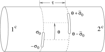
Fig. 17: The string diagram corresponding to the vertex $\langle v_{3}(\sigma_{0},\tilde{\sigma_{0}},\theta,\tau)|$.

Consider string configurations corresponding to the LPP vertex $\langle v_{3}(\sigma_{0},\tilde{\sigma_{0}},\theta,\tau)|$. We note that, for each possible configuration at $\tau=0$, there are always a pair of configurations with $\tau\not=0$ which reduce to the same configuration at $\tau=0$; they are clearly the two configurations with $(\sigma_{0}{=}x,\,\tilde{\sigma}_{0}{=}y,\,\theta{=}\phi)$ $(\sigma_{0}{=}y,\,\tilde{\sigma}_{0}{=}x,\,\theta{=}{-}\phi)$. Though the pair reduce to the same configuration, the anti-ghost factors $b_{\sigma_{0}}b_{\tilde{\sigma}_{0}}$ appear in the reverse order. Since anti-ghost factors anti-commute, the pair cancel each other and Eq. (5.56) becomes zero. We thus have proved that the order $g^{4}$ gauge invariance is realized.

6 String 2-point Amplitudes

In this section, we calculate closed string 2-point amplitudes corresponding to a disk and a projective plane using the Feynman rule which follows from the gauge invariant action determined in the previous section.

We must fix the gauge first. From the gauge invariance under the transformation of Eq. (1), it is possible to impose the usual gauge fixing condition for the closed string field;

$$b_{0}^{+}\left|\mathchar 28936\relax\right>=0.$$ (6.1)

The present open-closed mixed system is naturally expected to possess also the gauge symmetry with an open string field parameter $\mathchar 28931\relax^{\mathrm{o}}$, although we have not discussed it. (Actually, it is violated at the tree level but is realized at the loop level, as we shall see in later publication.[14]) So here we simply assume that this is the case and we impose the same type of gauge condition also for the open string field:

$$b_{0}\left|\mathchar 28937\relax\right>=0.$$ (6.2)

Once the gauge is fixed, we can derive the gauge fixed action and the Feynman rules following by now the standard procedure: the gauge fixed action takes the same form as the above gauge invariant one (4.2), but here $\left|\mathchar 28937\relax\right>$ and $\left|\mathchar 28936\relax\right>$ are now subject to the gauge conditions (6.2) and (6.1) and contain only the $\left|\phi\right>$ component defined in Eq. (2.5). (However, the $\left|\phi\right>$ here in the gauge fixed action contains much more component fields than the original $\left|\phi\right>$ (or even the whole fields $\left|\mathchar 28937\relax\right>$ and $\left|\mathchar 28936\relax\right>$) of the gauge invariant action, since now in the gauge fixed action the restriction that the component fields carry vanishing ghost number is no longer imposed. The infinite tower of component fields carrying non-zero ghost number here correspond to the FP ghost fields, ghosts’ ghost fields, and so on.)  The Feynman propagators are given by

$$\mathop{\vbox{\halign{#\cr\kern 1.72218pt\cr$\hbox{$\hskip 9.16669pt\vrule height=7.31946pt,width=0.29999pt,depth=-0.66708pt\kern-0.29999pt\vrule height=7.31946pt,width=21.13339pt,depth=-7.01947pt\kern-0.29999pt\vrule height=7.31946pt,width=0.29999pt,depth=-0.66708pt$}$ \crcr\kern 1.72218pt\nointerlineskip\cr\hbox{$\displaystyle\left|\mathchar 28937\relax\right>_{1}\left|\mathchar 28937\relax\right>_{2}$}\crcr}}}\limits=\left({b_{0}\over L_{0}}\right)^{(1)}\left|R^{\mathrm{o}}(1,2)\right>,$$ (6.5)

$$\mathop{\vbox{\halign{#\cr\kern 1.72218pt\cr$\hbox{$\hskip 15.98056pt\vrule height=7.31946pt,width=0.29999pt,depth=-0.66708pt\kern-0.29999pt\vrule height=7.31946pt,width=27.66948pt,depth=-7.01947pt\kern-0.29999pt\vrule height=7.31946pt,width=0.29999pt,depth=-0.66708pt$}$ \crcr\kern 1.72218pt\nointerlineskip\cr\hbox{$\displaystyle b_{0}^{-(1)}\left|\mathchar 28936\relax\right>_{1}{b_{0}^{-(2)}}\left|\mathchar 28936\relax\right>_{2}$}\crcr}}}\limits=\left({b_{0}{\bar{b}}_{0}\over L_{0}+\bar{L}_{0}}\right)^{(1)}\left|R^{\mathrm{c}}(1,2)\right>.$$ (6.8)

Note that these propagators indicate that only the $\left|\phi\right>$ components are propagating. Therefore, in the Feynman diagrams, we can use the same form of vertices as appearing in the gauge invariant action Eq. (4.2). [Precisely speaking, we should put the projections $\mathchar 28933\relax^{(1)}$ and $({\cal P}\mathchar 28933\relax)^{(1)}$ for the open and closed propagators, respectively, since our fields are subject to the constraints $\mathchar 28933\relax^{(1)}\left|\mathchar 28937\relax\right>=\left|\mathchar 28937\relax\right>$ and $({\cal P}\mathchar 28933\relax)^{(1)}\left|\mathchar 28936\relax\right>=\left|\mathchar 28936\relax\right>$. But, since all the vertices are constructed to contain those projections, we can omit them from the propagators.]

Now, we consider the disk amplitude for the closed tachyon 2-point function which comes from using the open-closed transition vertex twice. Noting that normalized closed tachyon state is given by

$$\left|\mathchar 28936\relax(p)\right>=\sqrt{2}c_{0}^{-}\left|\varphi(p)\right>,$$

$$\left|\varphi(p)\right>=\left[c(w){\bar{c}}({\bar{w}})\exp{\bigl{(}ip\cdot\hbox{${1\over 2}$}(X(w)+\bar{X}({\bar{w}}))\bigr{)}}\right]_{\scriptstyle w=0\atop\scriptstyle{\bar{w}}=0}\left|0\right>,$$ (6.9)

and satisfies ${\cal P}\mathchar 28933\relax\left|\varphi(p)\right>=\left|\varphi(p)\right>$, we find the disk amplitude as follows:

$$(2\pi)^{d}\delta^{d}(p_{1}+p_{2}){\cal A}_{D_{2}}$$

$$= (x_{u}g)^{2}\mathop{\vbox{\halign{#\cr\kern 1.72218pt\cr$\hbox{$\hskip 88.2938pt\vrule height=7.31946pt,width=0.29999pt,depth=-0.66708pt\kern-0.29999pt\vrule height=7.31946pt,width=100.2605pt,depth=-7.01947pt\kern-0.29999pt\vrule height=7.31946pt,width=0.29999pt,depth=-0.66708pt$}$ \crcr\kern 1.72218pt\nointerlineskip\cr\hbox{$\displaystyle\langle U(4,2^{\mathrm{c}})|{\left|\mathchar 28936\relax(p_{2})\right>}_{2^{\mathrm{c}}}\left|\mathchar 28937\relax\right>_{4}\langle U(3,1^{\mathrm{c}})|{\left|\mathchar 28936\relax(p_{1})\right>}_{1^{\mathrm{c}}}\left|\mathchar 28937\relax\right>_{3}$}\crcr}}}\limits$$

$$= 2x_{u}^{2}\,g^{2}\langle u(4,2^{\mathrm{c}})|\langle u(3,1^{\mathrm{c}})|\frac{{b_{0}}^{(4)}}{L_{0}^{(4)}}\left|R^{\mathrm{o}}(3,4)\right>\left|\varphi(p_{1})\right>_{1^{\mathrm{c}}}\left|\varphi(p_{2})\right>_{2^{\mathrm{c}}}$$

$$= 2x_{u}^{2}\,g^{2}\int_{0}^{\infty}d\tau\langle u(3,1^{\mathrm{c}})|\langle u(4,2^{\mathrm{c}})|$$

$$\qquad\times\oint_{C}\frac{d\rho}{2\pi i}\left({d\rho\over d\rho_{4}}\right)b(\rho)e^{-L_{0}^{(4)}\tau}\left|R^{\mathrm{o}}(3,4)\right>\left|\varphi(p_{1})\right>_{1^{\mathrm{c}}}\left|\varphi(p_{2})\right>_{2^{\mathrm{c}}}$$

$$= -4nx_{u}^{2}\,g^{2}\int_{0}^{\infty}d\tau\langle v_{D_{2}}(1^{\mathrm{c}},2^{\mathrm{c}};\,T{=}2\tau)|\oint_{C}\frac{d\rho}{2\pi i}b(\rho)\left|\varphi(p_{1})\right>_{1^{\mathrm{c}}}\left|\varphi(p_{2})\right>_{2^{\mathrm{c}}}\ ,$$ (6.13)

where $\langle v_{D_{2}}(1^{\mathrm{c}},2^{\mathrm{c}};\,T{=}2\tau)|$ is the LPP vertex introduced in Eq. (5.2) corresponding to Fig. 8 and the contour $C$ is the path traversing the intermediate open string strip (from bottom to top). Note that $d\rho/d\rho_{4}=\alpha_{4}=2$ was used since string 4 is an open string. The front minus sign in the last expression comes from the exchange of the order of $b(\rho)$ and $\left|R^{\mathrm{o}}(3,4)\right>$. By the definition of the LPP vertex and the mapping (5.17), we can evaluate the amplitude as follows by the conformal field theory on the $z$ plane in Fig. 11:

$$= -4n\,x_{u}^{2}\,g^{2}\,\delta^{d}(p_{1}+p_{2})\int_{0}^{\infty}d\tau\oint_{C^{\prime}}\frac{dz}{2\pi i}\left(\frac{d\rho}{dz}\right)^{-1}\left<b(z)c(Z_{1})c(\hat{Z}_{1})c(Z_{2})c(\hat{Z}_{2})\right>$$ (6.14)

$$\qquad\qquad\times\left<e^{ip_{1}\cdot X(Z_{1})/2}e^{ip_{1}\cdot X(\hat{Z}_{1})/2}e^{ip_{2}\cdot X(Z_{2})/2}e^{ip_{2}\cdot X(\hat{Z}_{2})/2}\right>,$$

where $d=26$ and the contour $C^{\prime}$ is the image of $C$ on the $z$ plane which is just the line from $i\infty$ to $-i\infty$ along the imaginary axis of the $z$ plane in Fig. 11. The correlation function for the ghost part is calculated in Appendix A, and the matter part is easily evaluated by using $\left<X^{\mu}(z)\,X^{\nu}(\tilde{z})\right>=-\eta^{\mu\nu}\ln(z-\tilde{z})$ as

$$\left<e^{ip_{1}\cdot X(Z_{1})/2}e^{ip_{1}\cdot X(\hat{Z}_{1})/2}e^{ip_{2}\cdot X(Z_{2})/2}e^{ip_{2}\cdot X(\hat{Z}_{2})/2}\right>$$

$$\qquad\qquad=\prod_{\stackrel{{\scriptstyle\scriptstyle r\neq s}}{{r,s=1,2,\hat{1},\hat{2}}}}(Z_{r}-Z_{s})^{p_{r}\cdot p_{s}/4}=\frac{(1-q^{2})^{2}}{2^{4}q^{4}},$$ (6.15)

where we have used the momentum conservation and the on-shell condition $p_{1}^{2}=p_{2}^{2}=8$ together with Eq. (5.20). Thus, using Eqs. (A.9) and (A.17) in the Appendix A, we find the disk amplitude as follows,

$${\cal A}_{D_{2}} = -4n\,x_{u}^{2}\,g^{2}\int_{0}^{\infty}d\tau\oint_{C^{\prime}}\frac{dz}{2\pi i}{\prod_{r=1,\hat{1},2,\hat{2}}(z-Z_{r})\over 4(z-z_{0}^{(1)})(z-z_{0}^{(2)})}{2^{6}q^{2}(1-q^{2})\over\prod_{r=1,\hat{1},2,\hat{2}}(z-Z_{r})}\frac{(1-q^{2})^{2}}{2^{4}q^{4}}$$ (6.16)

$$= -4n\,x_{u}^{2}\,g^{2}\int_{0}^{\infty}d\tau\frac{(1-q^{2})^{3}}{2q^{3}}=-4n\,x_{u}^{2}\,g^{2}\int_{0}^{1}dq\frac{1}{q^{3}}(1-q^{2})^{2},$$

where we have evaluated the $\oint_{C^{\prime}}dz/2\pi i$ integration simply by evaluating the residue at $z_{0}^{(1)}(=q)$, and then used $d\tau=d(T/2)=(2/(1-q^{2}))dq$ which follows from Eq. (5.14).

Similarly, we can calculate the projective plane amplitude for the tachyon 2-point function, which comes from the closed intersection vertex as follows:

$$(2\pi)^{d}\delta^{d}(p_{1}+p_{2}){\cal A}_{P_{2}}$$ (6.17)

$$= -x_{\infty}\,g^{2}\langle V_{\infty}(1^{\mathrm{c}},2^{\mathrm{c}})|\sqrt{2}{c_{0}^{-}}^{(1^{\mathrm{c}})}\left|\varphi(p_{1})\right>_{1^{\mathrm{c}}}\sqrt{2}{c_{0}^{-}}^{(2^{\mathrm{c}})}\left|\varphi(p_{2})\right>_{2^{\mathrm{c}}}$$

$$= -x_{\infty}\,g^{2}\,\int_{0}^{\pi/2}d\sigma_{0}\langle v_{\infty}(1^{\mathrm{c}},2^{\mathrm{c}};\sigma_{0})|b_{\sigma_{0}}\sqrt{2}\left|\varphi(p_{1})\right>_{1^{\mathrm{c}}}\sqrt{2}\left|\varphi(p_{2})\right>_{2^{\mathrm{c}}}$$

$$= -2x_{\infty}\,g^{2}\,\delta^{d}(p_{1}+p_{2})\int_{0}^{\pi/2}d\sigma_{0}\left(-i\oint_{C_{\hbox{$z$}_{0}^{\hbox{$(1)$}}}}+i\oint_{C_{\hbox{$z$}_{0}^{\hbox{$(2)$}}}}\right)\frac{dz}{2\pi i}\left(\frac{d\rho}{dz}\right)^{-1}$$

$$\qquad\times\left<b(z)c(Z_{1})c(\hat{Z}_{1})c(Z_{2})c(\hat{Z}_{2})\right>$$

$$\qquad\times\left<e^{ip_{1}\cdot X(Z_{1})/2}e^{ip_{1}\cdot X(\hat{Z}_{1})/2}e^{ip_{2}\cdot X(Z_{2})/2}e^{ip_{2}\cdot X(\hat{Z}_{2})/2}\right>$$

so that

$${\cal A}_{P_{2}} = -2x_{\infty}\,g^{2}\int_{0}^{\pi/2}d\sigma_{0}\left(-i\oint_{C_{\hbox{$z$}_{0}^{\hbox{$(1)$}}}}+i\oint_{C_{\hbox{$z$}_{0}^{\hbox{$(2)$}}}}\right)\frac{dz}{2\pi i}{1\over(z-z_{0}^{(1)})(z-z_{0}^{(2)})}{(1-q^{2})^{3}\over q^{2}}$$ (6.18)

$$= -2x_{\infty}\,g^{2}\int_{0}^{\pi/2}d\sigma_{0}\left(-i{1\over 2q}+i{1\over-2q}\right){(1-q^{2})^{3}\over q^{2}}$$

$$= +2x_{\infty}\,g^{2}\int_{0}^{\pi/2}id\sigma_{0}\frac{1}{q^{3}}(1-q^{2})^{3}=+2x_{\infty}\,g^{2}\int_{0}^{+i}dq\frac{2}{q^{3}}(1-q^{2})^{2}$$

$$= -4x_{\infty}\,g^{2}\int_{0}^{1}dq\frac{1}{q^{3}}(1+q^{2})^{2}.$$

where use has been made of $i\sigma_{0}=\ln[(1+q)/(1-q)]$ and $d(i\sigma_{0})=(2/(1-q^{2}))dq$, and, at the final step, we have changed the variable, $q\rightarrow iq$ so that the new $q$ takes real values in $[0,1]$ as in the preceding case.

The amplitudes of Eqs. (6.16) and (6.17) are singular at the point $q=0$, and so we introduce a cut-off parameter $a$:

$${\cal A}_{D_{2}\atop P_{2}} = -4g^{2}\left({nx_{u}^{2}\atop x_{\infty}}\right)\lim_{a\rightarrow 0}\int_{a}^{1}dq\frac{1}{q^{3}}(1\mp q^{2})^{2}$$ (6.19)

$$= -4g^{2}\left({nx_{u}^{2}\atop x_{\infty}}\right)\lim_{a\rightarrow 0}\left(\frac{1}{2a^{2}}\pm 2\ln a\right).$$

The quadratic divergences correspond to an emission of the closed tachyon to the vacuum, and the logarithmic divergence to the dilaton. The two dilaton divergences are combined to cancel each other if $x_{\infty}=nx_{u}^{2}$, which is the same condition as required by the gauge invariance in the previous section. So we are left with

$${\cal A}_{D_{2}}+{\cal A}_{P_{2}}=-\lim_{a\rightarrow 0}\frac{4nx_{u}^{2}}{a^{2}}\,g^{2}.$$ (6.20)

We still have another amplitude contribution to the same order, coming from the counter term which was introduced as a renormalization of the intercept. The counterterm is contained in ${\tilde{Q}}_{\rm B}^{\mathrm{c}}=Q_{\rm B}^{\mathrm{c}}+\lambda_{\mathrm{c}}g^{2}{c_{0}^{+}}$, and hence contributes to the tachyon amplitude as

$$(2\pi)^{d}\delta^{d}(p_{1}+p_{2}){\cal A}_{\rm count}$$ (6.21)

$$= -\langle R^{\mathrm{c}}(2^{\mathrm{c}},1^{\mathrm{c}})|\sqrt{2}{c_{0}^{-}}^{(1^{\mathrm{c}})}\left|\varphi(p_{1})\right>_{1^{\mathrm{c}}}\lambda_{\mathrm{c}}g^{2}{c_{0}^{+}}^{(2^{\mathrm{c}})}{b_{0}^{-}}^{(2^{\mathrm{c}})}\sqrt{2}{c_{0}^{-}}^{(2^{\mathrm{c}})}\left|\varphi(p_{2})\right>_{2^{\mathrm{c}}}$$

$$= -2\lambda_{\mathrm{c}}g^{2}\langle R^{\mathrm{c}}(2^{\mathrm{c}},1^{\mathrm{c}})|{c_{0}^{-}}^{(1^{\mathrm{c}})}\left|\varphi(p_{1})\right>_{1^{\mathrm{c}}}{c_{0}^{+}}^{(2^{\mathrm{c}})}\left|\varphi(p_{2})\right>_{2^{\mathrm{c}}}.$$

This is easily evaluated using the oscillator expression directly and yield

$${\cal A}_{\rm count}=-2\lambda_{\mathrm{c}}g^{2}=+\lim_{a\rightarrow 0}\frac{4nx_{u}^{2}}{a^{2}}g^{2}.$$ (6.22)

The cut-off parameter $a$ here is the one introduced in the previous section and has obviously the same physical meaning as that introduced in Eq. (6.19), and so we can identify these parameters. Comparing Eq. (6.20) and (6.22), it turns out that also the divergences originated in the tachyon cancel after summation of the three amplitudes if the action has the gauge symmetry, and we conclude that the net tachyon amplitude vanishes in this order:

$${\cal A}_{D_{2}}+{\cal A}_{P_{2}}+{\cal A}_{\rm count}=0.$$ (6.23)

7 Summary and discussion

In this paper we have considered the mixed system of open and closed strings and constructed the string field theory action explicitly up to the terms quadratic in the fields. We have proved in detail the invariance of the action under the gauge transformation with closed string field parameter $\mathchar 28931\relax^{\mathrm{c}}$.

It is not difficult, in principle, to construct the full action which is invariant under both type gauge transformations with open and closed string field parameters $\mathchar 28931\relax^{\mathrm{o}}$ and $\mathchar 28931\relax^{\mathrm{c}}$. But, to do this, we need to consider one-loop amplitudes with open-string external states. This is because of anomaly: the gauge invariance under the open string transformation parameter $\mathchar 28931\relax^{\mathrm{o}}$ is violated at one-loop diagrams for open string 2-point function constructed with 3-open-string-vertex twice. And those violations can be canceled by the tree diagrams with the open-closed transition interaction $U$ twice and with open intersection interaction $V_{\propto}$ once. [As for the orientable diagram parts, this anomaly is essentially the same as the situation for the Lorentz invariance known already in the light-cone gauge string field theory.[11, 12, 13]] The string diagrams between which these cancellations occur for non-orientable diagram parts are locally the same as the D2 and P2 diagrams in Figs. 8 and 6 considered in this paper, and the only difference is that there the external states are also open strings (so D2 becomes a one-loop diagram). It is there that the relation between the coupling constants $x_{\propto}$ and $x_{u}$ is fixed and the condition

$$n=2^{26/2}=8192$$ (7.1)

is required. Because of the complications due to loop-amplitude calculation, we deferred these discussions to the forthcoming paper in which we shall present the full gauge invariant action.

The main motive for this work is to develop the string field theory which can describe the D-branes. Since T-dual transformation of the usual open string gives the open string with Dirichlet boundary, the D-brane dynamics can be studied in detail in our string field theory for open-closed mixed system. But, to do this fully we have to wait for the completion of the full gauge invariant action. Even at this stage, however, we can see some connection of our string field theory and the Dirac-Born-Infeld action for D-branes. Let us explain this here briefly.

We consider the gauge transformations for some massless fields. If the T-duality transformation is done, the unoriented closed string is known to look like an oriented closed string apart from the orientifold plane,[31] and so it becomes to contain an anti-symmetric tensor field $B_{\mu\nu}(x)$ in the form

$$b_{0}^{-}\left|\mathchar 28936\relax\right> = \frac{1}{2}B_{\mu\nu}(x)\left(\alpha_{-1}^{\mu}\bar{\alpha}_{-1}^{\nu}-\alpha_{-1}^{\nu}\bar{\alpha}_{-1}^{\mu}\right)\left|1,1\right>+\cdots$$ (7.2)

$$= -\frac{1}{2}B_{\mu\nu}(x)\left[c\partial X^{\mu}(w){\bar{c}}\bar{\partial}\bar{X}^{\nu}({\bar{w}})-(\mu\leftrightarrow\nu)\right]_{\scriptstyle w=0\atop\scriptstyle{\bar{w}}=0}\left|0\right>+\cdots.$$

The transformation parameter $\mathchar 28931\relax^{\mathrm{c}}$ has the following mode:

$$b_{0}^{-}\left|\mathchar 28931\relax^{\mathrm{c}}\right> = -2i\zeta_{\mu}(x)\left(b_{-1}\bar{\alpha}_{-1}^{\mu}-\bar{b}_{-1}\alpha_{-1}^{\mu}\right)\left|1,1\right>+\cdots$$ (7.3)

$$= 2\zeta_{\mu}(x)\left[c\partial X^{\mu}(w)+{\bar{c}}\bar{\partial}\bar{X}^{\mu}({\bar{w}})\right]_{\scriptstyle w=0\atop\scriptstyle{\bar{w}}=0}\left|0\right>+\cdots.$$

Noting that the last expression can also be written as

$$2\left[\zeta_{\mu}\bigl{(}\hbox{${1\over 2}$}(X(w)+\bar{X}({\bar{w}}))\bigr{)}\left(c\partial X^{\mu}(w)+{\bar{c}}\bar{\partial}\bar{X}^{\mu}({\bar{w}})\right)\right]_{\scriptstyle w=0\atop\scriptstyle{\bar{w}}=0}\left|0\right>$$ (7.4)

(with normal ordering implied) and that $[Q_{\rm B},\,X]=c\partial X$ and $[Q_{\rm B},\,\bar{X}]={\bar{c}}\bar{\partial}\bar{X}$, we find the BRS transform of this as

$$-Q_{\rm B}b_{0}^{-}\left|\mathchar 28931\relax^{\mathrm{c}}\right> = -\frac{1}{2}\left(\partial_{\mu}\zeta_{\nu}(x)-\partial_{\nu}\zeta_{\mu}(x)\right)$$ (7.5)

$$\qquad\times\left[c\partial X^{\mu}(w){\bar{c}}\bar{\partial}\bar{X}^{\nu}({\bar{w}})-(\mu\leftrightarrow\nu)\right]_{\scriptstyle w=0\atop\scriptstyle{\bar{w}}=0}\left|0\right>+\cdots.$$

Then the anti-symmetric tensor field is transformed under the gauge transformation of Eq. (1) at the leading order as follows,

$$\delta B_{\mu\nu}=\partial_{\mu}\zeta_{\nu}-\partial_{\nu}\zeta_{\mu}.$$ (7.6)

Next consider the gauge transformation for an open string massless gauge mode generated by the same parameter of Eq. (7.3). The massless gauge field $A_{\mu}$ is contained in the open string field as

$$\left|\mathchar 28937\relax\right> = -iA_{\mu}(x)\alpha_{-1}^{\mu}\left|1\right>+\cdots$$ (7.7)

$$= A_{\mu}(x)[c\partial X^{\mu}(w)]_{w=0}\left|0\right>+\cdots.$$

From this equation, we can find the gauge transformation for the massless mode by

$$\delta A^{\mu} = i\langle 1|c_{0}\alpha^{\mu}_{1}\left(\delta\left|\mathchar 28937\relax\right>\right).$$ (7.8)

On a (group) symmetric background, only the trace part of the open string field gets transformed under the gauge transformation Eq. (4). The gauge modes belong to the adjoint representation, which is anti-symmetric and has no trace part in the present O($n$) case, and hence receives no transformation under the closed parameter gauge transformation. But, if a non-trivial Wilson line background appears (which gives rise to the coordinates of the D-branes), then, the gauge field components corresponding to the Cartan subalgebra become to receive the same form of gauge transformation as in Eq. (4) without taking trace. Assuming this, the gauge transformation of a Cartan subalgebra component of the gauge field is given by

$$\delta A^{\mu}\propto{\textstyle{\atop 1}}\!\langle 1|{c_{0}}^{(1)}{\alpha_{1}^{\mu}}^{(1)}\langle U(2,1^{\mathrm{c}})|\left|R^{\mathrm{o}}(1,2)\right>\left|\mathchar 28931\relax^{\mathrm{c}}\right>_{1^{\mathrm{c}}},$$ (7.9)

with the understanding that $\langle U(2,1^{\mathrm{c}})|\left|R^{\mathrm{o}}(1,2)\right>$ now does not imply taking the trace.

Fig. 12: Contour deformations a) and b) used in Eqs. (5.46) and (5.49), respectively.

 

In order to evaluate this, it is convenient to map the $\rho$ plane in Fig. 2 of the open-closed transition vertex to the $z$ plane in Fig. Unoriented Open-Closed String Field Theory by the following Mandelstam mapping:

$$\rho=\ln(z-ib)+\ln(z+ib).$$ (7.10)

On the $z$ plane, the real axis corresponds to the open string boundary. $Z_{1}=+ib$ and $\hat{Z}_{1}=-ib$ correspond to the closed string insertion points, and $Z_{2}=\infty$ to the open string insertion point. We can evaluate the gauge transformation as follows: Substituting Eq. (7.3) into Eq. (7.9), and going to the $z$ plane, we find

$$\delta A^{\mu} \propto \hbox{${1\over 2}$}\bigl{\langle}\zeta_{\nu}\bigl{(}\hbox{${1\over 2}$}(X(Z_{1})+X(\hat{Z}_{1}))\bigr{)}\left(c\partial X^{\nu}(Z_{1})+c\partial X^{\nu}(\hat{Z}_{1})\right)c\partial c\partial X^{\mu}(Z_{2})\bigr{\rangle}$$ (7.11)

$$= -\zeta^{\mu}(x).$$

The gauge transformations (7.6) and (7.11) are of the same form as those in the Dirac-Born-Infeld action, and so the open-closed string field theory possesses the symmetry of the Dirac-Born-Infeld action as a part of its gauge symmetry.

A Relation between the LPP, KS and HIKKO vertices

We prove Eq. (5.21) in this appendix. So the discussion is performed on the concrete case of two closed string vertices, but it will also clarifies general relations between the three apparently different expressions for the vertices given by LPP, KS and HIKKO.

Let us denote the LPP’s D2 vertex $\langle v_{D_{2}}(1^{\mathrm{c}},2^{\mathrm{c}};T)|$ and P2 vertex $\langle V_{\infty}(1^{\mathrm{c}},2^{\mathrm{c}};\sigma_{0})|$ unifiedly by

$$\langle v(1^{\mathrm{c}},2^{\mathrm{c}};q)|.$$ (A.1)

Namely, this corresponds to the configuration Fig. 8 for real $q=a$ and Fig. 6 for imaginary $q=ia$, respectively. These $\rho$ planes are mapped to the $z$ planes in Fig. 11 and Fig. 11, respectively, via the mapping Eq. (5.17).

By the definition of the LPP vertex, we have

$$\langle v(1^{\mathrm{c}},2^{\mathrm{c}};q)|{\cal O}(z)\cdots\,\left|1,1\right>_{1^{\mathrm{c}}}\left|1,1\right>_{2^{\mathrm{c}}}=\left(\frac{dZ_{1}}{dw_{1}}\right)^{-1}\left(\frac{d\hat{Z}_{1}}{d\bar{w}_{1}}\right)^{-1}\left(\frac{dZ_{2}}{dw_{2}}\right)^{-1}\left(\frac{d\hat{Z}_{2}}{d\bar{w}_{2}}\right)^{-1}$$

$$\hskip 120.00018pt\times\left<\,{\cal O}(z)\cdots\,c(Z_{1})c(\hat{Z}_{1})c(Z_{2})c(\hat{Z}_{2})\right>,$$ (A.2)

for any operators ${\cal O}(z)\cdots$, where $\langle\ \ \rangle$ denotes the correlation function of the conformal field theory on the $z$ plane and the factors

$$\left(\frac{dZ_{r}}{dw_{r}}\right)^{-1}=\lim_{z\rightarrow Z_{r}}\left(\frac{dz}{dw_{r}}\right)^{-1},\hskip 10.00002pt\pmatrix{Z_{r}=Z_{1},\,\hat{Z}_{1},\,Z_{2},\,\hat{Z}_{2}\cr w_{r}=w_{1},\,\bar{w}_{1},\,w_{2},\,\bar{w}_{2}\cr},$$ (A.3)

appear from the conformal mapping of the ghost factors contained in the Fock vacuum; $\left|1,1\right>=c(w{=}0){\bar{c}}({\bar{w}}{=}0)\left|0,0\right>$. Henceforth, we use the notation $\left|\bf 1\right>_{1^{\mathrm{c}},2^{\mathrm{c}}}$ to denote $\left|1,1\right>_{1^{\mathrm{c}}}\left|1,1\right>_{2^{\mathrm{c}}}$, for brevity.

On the other hand, Kunitomo and Suehiro have defined in Ref. ? the vertex by the condition:

$$\langle V_{\rm KS}(1^{\mathrm{c}},2^{\mathrm{c}};z_{0}^{(s)})|c(z)b(\tilde{z})\left|\bf 1\right>_{1^{\mathrm{c}},2^{\mathrm{c}}} = \frac{\left<b(z_{0}^{(s)})c(z)b(\tilde{z})c(Z_{1})c(\hat{Z}_{1})c(Z_{2})c(\hat{Z}_{2})\right>}{\left<b(z_{0}^{(s)})c(Z_{1})c(\hat{Z}_{1})c(Z_{2})c(\hat{Z}_{2})\right>}$$ (A.4)

$$= \frac{1}{z-\tilde{z}}\,\frac{\tilde{z}-z_{0}^{(s)}}{z-z_{0}^{(s)}}\prod_{r=1,\hat{1},2,\hat{2}}\frac{z-Z_{r}}{\tilde{z}-Z_{r}},$$

where $z_{0}^{(s)}$ denotes one of the two interaction points $z_{0}^{(1)}$ and $z_{0}^{(2)}$ on the $z$ plane, on which the KS vertex depends. The KS vertex satisfies the normalization condition $\langle V_{\rm KS}(1^{\mathrm{c}},2^{\mathrm{c}};z_{0}^{(s)})|\left|\bf 1\right>_{1^{\mathrm{c}},2^{\mathrm{c}}}=1$ by this definition. It is important that, as KS noted, the information of the two point function of this type is enough to determine the vertex.

If we take $b(z_{0}^{(s)})\,c(z)b(\tilde{z})$ for ${\cal O}(z)\cdots$ in Eq. (A), we have

$$\langle v(1^{\mathrm{c}},2^{\mathrm{c}};q)|b(z_{0}^{(s)})\,c(z)b(\tilde{z})\left|\bf 1\right>_{1^{\mathrm{c}},2^{\mathrm{c}}}$$

$$\quad=\left(\frac{dZ_{1}}{dw_{1}}\frac{d\hat{Z}_{1}}{d\bar{w}_{1}}\frac{dZ_{2}}{dw_{2}}\frac{d\hat{Z}_{2}}{d\bar{w}_{2}}\right)^{-1}\left<\,b(z_{0}^{(s)})\,c(z)b(\tilde{z})\,c(Z_{1})c(\hat{Z}_{1})c(Z_{2})c(\hat{Z}_{2})\right>.$$ (A.5)

Comparing this with Eq. (A.4), we see that the KS vertex $\langle V_{\rm KS}(1^{\mathrm{c}},2^{\mathrm{c}};z_{0}^{(s)})|$ coincides with $\langle v(1^{\mathrm{c}},2^{\mathrm{c}};q)|b(z_{0}^{(s)})$ up to a proportional factor depending on the moduli $q$:

$$\langle v(1^{\mathrm{c}},2^{\mathrm{c}};q)|b(z_{0}^{(s)})={\cal N}(q)\langle V_{\rm KS}(1^{\mathrm{c}},2^{\mathrm{c}};z_{0}^{(s)})|,$$ (A.6)

where ${\cal N}(q)$ can be found by multiplying $\left|\bf 1\right>_{1^{\mathrm{c}},2^{\mathrm{c}}}$ on both sides of this as

$${\cal N}(q) = \langle v(1^{\mathrm{c}},2^{\mathrm{c}};q)|b(z_{0}^{(s)})\left|\bf 1\right>_{1^{\mathrm{c}},2^{\mathrm{c}}}$$ (A.7)

$$= \left(\frac{dZ_{1}}{dw_{1}}\frac{d\hat{Z}_{1}}{d\bar{w}_{1}}\frac{dZ_{2}}{dw_{2}}\frac{d\hat{Z}_{2}}{d\bar{w}_{2}}\right)^{-1}\left<\,b(z_{0}^{(s)})c(Z_{1})c(\hat{Z}_{1})c(Z_{2})c(\hat{Z}_{2})\right>.$$ (A.8)

Each factor of this can be calculated as follows: using

$$\left<(b(z)c(Z_{1})c(Z_{2})c(Z_{3})c(Z_{4})\right> = \det\pmatrix{\displaystyle{1\over z-Z_{1}}&\displaystyle{1\over z-Z_{2}}&\displaystyle{1\over z-Z_{3}}&\displaystyle{1\over z-Z_{4}}\cr Z_{1}^{2}&Z_{2}^{2}&Z_{3}^{2}&Z_{4}^{2}\cr Z_{1}&Z_{2}&Z_{3}&Z_{4}\cr 1&1&1&1\cr}$$ (A.9)

$$= -{\prod_{1\leq i<j\leq 4}(Z_{i}-Z_{j})\over\prod_{r=1}^{4}(z-Z_{r})}$$

and Eqs. (5.18) and (5.20) for $z_{0}^{(s)}$ and $Z_{1},\hat{Z}_{1},Z_{2},\hat{Z}_{2}$, we find

$$\left<(b(z_{0}^{(s)})c(Z_{1})c(\hat{Z}_{1})c(Z_{2})c(\hat{Z}_{2})\right>=-{-2^{6}q^{2}(1-q^{2})\over 2^{2}q^{2}(q^{2}-1)}=-2^{4}.$$ (A.10)

From Eq. (5.17) and $\rho=\alpha_{r}\ln w_{r}$ with $\alpha_{r}=+1$ $(-1)$ for $r=1,\hat{1}$ ($2,\hat{2}$), we have

$${dw_{r}\over dz}={-4\alpha_{r}z^{2}\over(z^{2}+2\alpha_{r}z+q^{2})^{2}}\left(1-{q^{2}\over z^{2}}\right).$$ (A.11)

Putting $z=Z_{1},\hat{Z}_{1},Z_{2},\hat{Z}_{2}$ and using (5.20), we find

$$\left(\frac{dZ_{1}}{dw_{1}}\frac{d\hat{Z}_{1}}{d\bar{w}_{1}}\frac{dZ_{2}}{dw_{2}}\frac{d\hat{Z}_{2}}{d\bar{w}_{2}}\right)^{-1}={1\over 4^{4}}\prod_{r=1,\hat{1},2,\hat{2}}\left(1-{q^{2}\over Z_{r}^{2}}\right)={(1-q^{2})^{2}\over 2^{4}q^{4}}.$$ (A.12)

So we obtain

$${\cal N}(q)=-{(1-q^{2})^{2}\over q^{4}}.$$ (A.13)

Now that the relation between the LPP and KS vertices is established, we can next clarify the relation between the KS and HIKKO vertices. Guided by the OSP($d,2|2$) symmetry, HIKKO defined the following ghost fields on the $z$ plane in their papers ?, ?:

$$c_{\mathrm{H}}(z)=\left(\frac{dz}{d\rho}\right)^{-1}c(z),\qquad b_{\mathrm{H}}(z)=\left(\frac{dz}{d\rho}\right)b(z),$$ (A.14)

or equivalently, in terms of the original fields on the $\rho$ plane, by

$$c_{\mathrm{H}}(z)=c(\rho),\qquad b_{\mathrm{H}}(z)=\left({d\rho\over dz}\right)b(\rho).$$ (A.15)

Namely, HIKKO treated the ghost fields as if $c$ and $b$ carry the weights 0 and +1, respectively, with which they could obtain OSp symmetric expression for the vertex.

We first note that the KS vertex realizes the following 2-point function for the HIKKO’s ghost fields:

$$\langle V_{\rm KS}(1^{\mathrm{c}},2^{\mathrm{c}};z_{0}^{(1)})|{\rm T}c_{\mathrm{H}}(z)b_{\mathrm{H}}(\tilde{z})\left|\bf 1\right>_{1^{\mathrm{c}},2^{\mathrm{c}}}$$

$$\qquad=\langle V_{\rm KS}(1^{\mathrm{c}},2^{\mathrm{c}};z_{0}^{(1)})|{\rm T}c(z)b(\tilde{z})\left|\bf 1\right>_{1^{\mathrm{c}},2^{\mathrm{c}}}\left({dz\over d\rho}\right)^{-1}\left({d\tilde{z}\over d\tilde{\rho}}\right)$$

$$\qquad=\frac{1}{z-\tilde{z}}\,\frac{z-z_{0}^{(2)}}{\tilde{z}-z_{0}^{(2)}},$$ (A.16)

as well as the same form of equation with the two interaction points $z_{0}^{(1)}$ and $z_{0}^{(2)}$ being interchanged, where use has been made of the definitions of KS vertex and HIKKO’s field, Eqs. (A.4) and (A.14), and the relation:

$${d\rho\over dz}={4(z-z_{0}^{(1)})(z-z_{0}^{(2)})\over\prod_{r=1,\hat{1},2,\hat{2}}(z-Z_{r})}.$$ (A.17)

Looking at this 2-point function in Eq. (A.16), we can guess that the KS vertex is given in the form:

$$\langle V_{\rm KS}(1^{\mathrm{c}},2^{\mathrm{c}};z_{0}^{(1)})|={\textstyle{\atop 2^{\mathrm{c}},1^{\mathrm{c}}}}\!\langle\tilde{\bf 1}|\left(\sum_{r=1,\hat{1},2,\hat{2}}\frac{b_{0}^{(r)}}{\alpha_{r}}\right)\exp(E_{\mathrm{H}}(1^{\mathrm{c}},2^{\mathrm{c}}))\,c_{\mathrm{H}}(z_{0}^{(2)})$$ (A.18)

(and the same form equation with $z_{0}^{(1)}$ and $z_{0}^{(2)}$ interchanged), where $E_{\mathrm{H}}$ is the HIKKO’s OSp symmetric quadratic operator written by annihilation operators alone, the explicit form of which will be given later in Eq. (5.22). The vacuum ${\textstyle{\atop 2^{\mathrm{c}},1^{\mathrm{c}}}}\!\langle\tilde{\bf 1}|$ here is the abbreviation for ${\textstyle{\atop 2^{\mathrm{c}}}}\!\langle\tilde{1},\tilde{1}|{\textstyle{\atop 1^{\mathrm{c}}}}\!\langle\tilde{1},\tilde{1}|$, and the bra vacuum $\langle\tilde{1},\tilde{1}|$ denotes $\langle\tilde{1},\tilde{1}|=\langle 1,1|c_{0}{\bar{c}}_{0}$ conjugate to the ket Fock vacuum $\left|1,1\right>$: $\langle\tilde{1},\tilde{1}|1,1\rangle=1$. Since the bra vacuum $\langle\tilde{1},\tilde{1}|$ is annihilated by $c_{0}$ and ${\bar{c}}_{0}$ and the ket vacuum $\left|1,1\right>$ by $b_{0}$ and ${\bar{b}}_{0}$, so we call $c_{0},{\bar{c}}_{0}$ creation operators and $b_{0},{\bar{b}}_{0}$ annihilation operators, henceforth.

From now on we prove Eq. (A.18); namely, the right-hand side of (A.18) also realizes the same 2-point function as in Eq. (A.16).

Noting that $E_{\mathrm{H}}$ is a quadratic form of annihilation operators alone, we have the following equation generally for operators ${\cal O}$ linear in the creation and annihilation operators:

$$e^{E_{\mathrm{H}}}\left\{{\cal O}_{1}{\cal O}_{2}\cdots\right\}=\bigl{\{}\left({\cal O}_{1}+[E_{\mathrm{H}},\,{\cal O}_{1}]\right)\left({\cal O}_{2}+[E_{\mathrm{H}},\,{\cal O}_{1}]\right)\cdots\bigr{\}}e^{E_{\mathrm{H}}}.$$ (A.19)

Now introduce the following notations,

$$\hat{{\cal O}}\equiv{\cal O}+[E_{\mathrm{H}},\,{\cal O}]=\hat{{\cal O}}^{(-)}+\hat{{\cal O}}^{(+)},$$

$$\hat{{\cal O}}^{(-)}\equiv{\cal O}^{(-)},\qquad\hat{{\cal O}}^{(+)}\equiv{\cal O}^{(+)}+[E_{\mathrm{H}},\,{\cal O}^{(-)}],$$ (A.20)

where superscripts $(-)$ and $(+)$ denote the creation and annihilation operator parts, respectively. The hatted operators are also linear in the creation and annihilation operators. Applying the Wick theorem to the hatted operators $\hat{\cal O}$, we have

$$e^{E_{\mathrm{H}}}{\rm T}\left({\cal O}_{1}{\cal O}_{2}{\cal O}_{3}\cdots\right)={\rm T}\left(\hat{{\cal O}_{1}}\hat{{\cal O}_{2}}\hat{{\cal O}_{3}}\cdots\right)e^{E_{\mathrm{H}}}$$

$$\qquad=\left(:\hat{{\cal O}_{1}}\hat{{\cal O}_{2}}\hat{{\cal O}_{3}}\cdots:+:\mathop{\vbox{\halign{#\cr\kern 1.72218pt\cr$\hbox{$\hskip 2.77779pt\vrule height=7.31946pt,width=0.29999pt,depth=-0.38931pt\kern-0.29999pt\vrule height=7.31946pt,width=8.35558pt,depth=-7.01947pt\kern-0.29999pt\vrule height=7.31946pt,width=0.29999pt,depth=-0.38931pt$}$ \crcr\kern 1.72218pt\nointerlineskip\cr\hbox{$\displaystyle\hat{\cal O}_{1}\hat{\cal O}_{2}$}\crcr}}}\limits{\hat{\cal O}_{3}}\cdots:+\ \cdots\ \right)e^{E_{\mathrm{H}}},$$ (A.23)

with the contraction of the $\hat{\cal O}$ operators given by

$$\mathop{\vbox{\halign{#\cr\kern 1.72218pt\cr$\hbox{$\hskip 2.77779pt\vrule height=7.31946pt,width=0.29999pt,depth=-0.38931pt\kern-0.29999pt\vrule height=7.31946pt,width=8.35558pt,depth=-7.01947pt\kern-0.29999pt\vrule height=7.31946pt,width=0.29999pt,depth=-0.38931pt$}$ \crcr\kern 1.72218pt\nointerlineskip\cr\hbox{$\displaystyle\hat{\cal O}_{1}\hat{\cal O}_{2}$}\crcr}}}\limits={\textstyle{\atop 2^{\mathrm{c}},1^{\mathrm{c}}}}\!\langle\tilde{\bf 1}|{\rm T}\hat{{\cal O}_{1}}\hat{{\cal O}_{2}}\left|\bf 1\right>_{1^{\mathrm{c}},2^{\mathrm{c}}}=\mathop{\vbox{\halign{#\cr\kern 1.72218pt\cr$\hbox{$\hskip 3.8889pt\vrule height=3.65973pt,width=0.29999pt,depth=-0.0004pt\kern-0.29999pt\vrule height=3.65973pt,width=10.5778pt,depth=-3.35974pt\kern-0.29999pt\vrule height=3.65973pt,width=0.29999pt,depth=-0.0004pt$}$ \crcr\kern 1.72218pt\nointerlineskip\cr\hbox{$\displaystyle{\cal O}_{1}{\cal O}_{2}$}\crcr}}}\limits+\bigl{[}[E_{\mathrm{H}},\,{\cal O}_{1}^{(-)}],\,{\cal O}_{2}^{(-)}\bigr{]}.$$ (A.24)

This contraction of the hatted operators is of just the same form as defined by HIKKO. Then, we obtain

$${\textstyle{\atop 2^{\mathrm{c}},1^{\mathrm{c}}}}\!\langle\tilde{\bf 1}|\left(\sum_{r}\frac{b_{0}^{(r)}}{\alpha_{r}}\right)e^{E_{\mathrm{H}}}\,{\rm T}\,c_{\mathrm{H}}(z_{0}^{(2)})c_{\mathrm{H}}(z)b_{\mathrm{H}}(\tilde{z})$$

$$\hskip 20.00003pt={\textstyle{\atop 2^{\mathrm{c}},1^{\mathrm{c}}}}\!\langle\tilde{\bf 1}|\left(\sum_{r}\frac{b_{0}^{(r)}}{\alpha_{r}}\right)\bigl{[}\mathop{\vbox{\halign{#\cr\kern 1.72218pt\cr$\hbox{$\hskip 2.77779pt\vrule height=7.31946pt,width=0.29999pt,depth=-0.38931pt\kern-0.29999pt\vrule height=7.31946pt,width=48.04735pt,depth=-7.01947pt\kern-0.29999pt\vrule height=7.31946pt,width=0.29999pt,depth=-0.38931pt$}$ \crcr\kern 1.72218pt\nointerlineskip\cr\hbox{$\displaystyle\hat{c}_{\mathrm{H}}(z_{0}^{(2)})\hat{c}_{\mathrm{H}}(z)\hat{b}_{\mathrm{H}}(\tilde{z})$}\crcr}}}\limits+\mathop{\vbox{\halign{#\cr\kern 1.72218pt\cr$\hbox{$\hskip 28.20146pt\vrule height=7.31946pt,width=0.29999pt,depth=-0.38931pt\kern-0.29999pt\vrule height=7.31946pt,width=22.62367pt,depth=-7.01947pt\kern-0.29999pt\vrule height=7.31946pt,width=0.29999pt,depth=-0.38931pt$}$ \crcr\kern 1.72218pt\nointerlineskip\cr\hbox{$\displaystyle\hat{c}_{\mathrm{H}}(z_{0}^{(2)})\hat{c}_{\mathrm{H}}(z)\hat{b}_{\mathrm{H}}(\tilde{z})$}\crcr}}}\limits$$ (A.29)

$$\hskip 130.0002pt+:{\hat{c}}_{\mathrm{H}}(z_{0}^{(2)}){\hat{c}}_{\mathrm{H}}(z){\hat{b}}_{\mathrm{H}}(\tilde{z}):\bigr{]}e^{E_{\mathrm{H}}}.$$ (A.30)

If $E_{\mathrm{H}}$ is such a quadratic form that it realizes

$$\mathop{\vbox{\halign{#\cr\kern 1.72218pt\cr$\hbox{$\hskip 2.77779pt\vrule height=7.31946pt,width=0.29999pt,depth=-0.38931pt\kern-0.29999pt\vrule height=7.31946pt,width=22.62367pt,depth=-7.01947pt\kern-0.29999pt\vrule height=7.31946pt,width=0.29999pt,depth=-0.38931pt$}$ \crcr\kern 1.72218pt\nointerlineskip\cr\hbox{$\displaystyle\hat{c}_{\mathrm{H}}(z)\hat{b}_{\mathrm{H}}(\tilde{z})$}\crcr}}}\limits=\frac{1}{z-\tilde{z}},$$ (A.33)

then, with the help of the formula (A.23), Eq. (A) becomes

$$={\textstyle{\atop 2^{\mathrm{c}},1^{\mathrm{c}}}}\!\langle\tilde{\bf 1}|\left(\sum_{r}\frac{b_{0}^{(r)}}{\alpha_{r}}\right)\left[-\frac{1}{z_{0}^{(2)}-\tilde{z}}\hat{c}_{\mathrm{H}}(z)+\frac{1}{z-\tilde{z}}\hat{c}_{\mathrm{H}}(z_{0}^{(2)})+:{\hat{c}}_{\mathrm{H}}(z_{0}^{(2)}){\hat{c}}_{\mathrm{H}}(z){\hat{b}}_{\mathrm{H}}(\tilde{z}):\right]e^{E_{\mathrm{H}}}.$$

Acting the Fock vacuum $\left|\bf 1\right>_{1^{\mathrm{c}},2^{\mathrm{c}}}$ on this equation, we have

$${\textstyle{\atop 2^{\mathrm{c}},1^{\mathrm{c}}}}\!\langle\tilde{\bf 1}|\left(\sum_{r}\frac{b_{0}^{(r)}}{\alpha_{r}}\right)e^{E_{\mathrm{H}}}c_{\mathrm{H}}(z_{0}^{(2)})\,{\rm T}\,c_{\mathrm{H}}(z)b_{\mathrm{H}}(\tilde{z})\left|\bf 1\right>_{1^{\mathrm{c}},2^{\mathrm{c}}}$$

$$\quad={\textstyle{\atop 2^{\mathrm{c}},1^{\mathrm{c}}}}\!\langle\tilde{\bf 1}|\left(\sum_{r}\frac{b_{0}^{(r)}}{\alpha_{r}}\right)\left[-\frac{1}{z_{0}^{(2)}-\tilde{z}}\hat{c}_{\mathrm{H}}(z)+\frac{1}{z-\tilde{z}}\hat{c}_{\mathrm{H}}(z_{0}^{(2)})\right]\left|\bf 1\right>_{1^{\mathrm{c}},2^{\mathrm{c}}}.$$ (A.34)

Since $b_{0}^{(r)}$ are the annihilation operators, only the $c_{0}$ mode part in $\hat{c}_{\mathrm{H}}(z)$ and $\hat{c}_{\mathrm{H}}(z_{0}^{(2)})$ can survive the VEV in the the right hand side. Noting

$$c_{\mathrm{H}}(z)=\alpha_{r}\sum_{n}{c_{n}}^{(r)}e^{in\rho_{r}}=\alpha_{r}c_{0}^{(r)}+(\hbox{non-zero modes}),$$ (A.35)

we have

$${\textstyle{\atop 2^{\mathrm{c}},1^{\mathrm{c}}}}\!\langle\tilde{\bf 1}|\left(\sum_{r}\frac{b_{0}^{(r)}}{\alpha_{r}}\right)\hat{c}_{\mathrm{H}}(z)\left|\bf 1\right>_{1^{\mathrm{c}},2^{\mathrm{c}}}={\textstyle{\atop 2^{\mathrm{c}},1^{\mathrm{c}}}}\!\langle\tilde{\bf 1}|\left(\sum_{r}\frac{b_{0}^{(r)}}{\alpha_{r}}\right)\hat{c}_{\mathrm{H}}(z_{0}^{(2)})\left|\bf 1\right>_{1^{\mathrm{c}},2^{\mathrm{c}}}=1,$$ (A.36)

so that Eq. (A) finally becomes

$$=-\frac{1}{z_{0}^{(2)}-\tilde{z}}+\frac{1}{z-\tilde{z}}=\frac{1}{z-\tilde{z}}\,\frac{z-z_{0}^{(2)}}{\tilde{z}-z_{0}^{(2)}}.$$ (A.37)

This is just equal to the right hand side of Eq. (A.16) and therefore, the Eq. (A.18) is proved. $E_{H}$ is determined by the requirement of

$$\mathop{\vbox{\halign{#\cr\kern 1.72218pt\cr$\hbox{$\hskip 2.16377pt\vrule height=3.65973pt,width=0.29999pt,depth=2.52737pt\kern-0.29999pt\vrule height=3.65973pt,width=21.37772pt,depth=-3.35974pt\kern-0.29999pt\vrule height=3.65973pt,width=0.29999pt,depth=-0.11153pt$}$ \crcr\kern 1.72218pt\nointerlineskip\cr\hbox{$\displaystyle c_{\mathrm{H}}(z)b_{\mathrm{H}}(\tilde{z})$}\crcr}}}\limits+\bigl{[}[E_{\mathrm{H}},\,c_{\mathrm{H}}(z)],\,b_{\mathrm{H}}(\tilde{z})\bigr{]}=\frac{1}{z-\tilde{z}}.$$ (A.40)

But HIKKO already showed that such $E_{H}$ is just given by the OSp invariant quadratic form given in Eq. (5.22).[18, 19]

Combining Eqs. (A.18) and (A.6), we find a direct relation between the LPP and HIKKO vertices:

$$\langle v(1^{\mathrm{c}},2^{\mathrm{c}};q)|b(z_{0}^{(1)})={\cal N}(q){\textstyle{\atop 2^{\mathrm{c}},1^{\mathrm{c}}}}\!\langle\tilde{\bf 1}|\left(\sum_{r=1,\hat{1},2,\hat{2}}\frac{b_{0}^{(r)}}{\alpha_{r}}\right)\exp(E_{\mathrm{H}}(1^{\mathrm{c}},2^{\mathrm{c}}))\,c_{\mathrm{H}}(z_{0}^{(2)}).$$ (A.41)

The same form equation with $z_{0}^{(1)}$ and $z_{0}^{(2)}$ interchanged also holds. To convert this into the desired Eq. (5.21), we note that

$$\langle v(1^{\mathrm{c}},2^{\mathrm{c}};q)|b(z_{0}^{(1)})c_{\mathrm{H}}(z_{0}^{(1)})=\lim_{z\rightarrow z_{0}^{(1)}}\langle v(1^{\mathrm{c}},2^{\mathrm{c}};q)|b(z_{0}^{(1)})c(z)\left({dz\over d\rho}\right)^{-1}$$

$$\qquad\qquad=\lim_{z\rightarrow z_{0}^{(1)}}\langle v(1^{\mathrm{c}},2^{\mathrm{c}};q)|\left({1\over z_{0}^{(1)}-z}+:b(z_{0}^{(1)})c(z):\right){4(z-z_{0}^{(1)})(z-z_{0}^{(2)})\over\displaystyle\prod_{r=1,\hat{1},2,\hat{2}}(z-Z_{r})}$$

$$\qquad\qquad={2\over q(1-q^{2})}\cdot\langle v(1^{\mathrm{c}},2^{\mathrm{c}};q)|,$$ (A.42)

where we have used Eq. (A.17), and Eqs. (5.18) and (5.20) for $z_{0}^{(s)}$ and $Z_{1},\hat{Z}_{1},Z_{2},\hat{Z}_{2}$. Thus, multiplying both sides of Eq. (A.41) by $-c_{\mathrm{H}}(z_{0}^{(1)})$, we can really obtain the desired expression Eq. (5.21) with the coefficient

$$N(q)=-{(1-q^{2})^{2}\over q^{4}}\times{q(1-q^{2})\over 2}\times(-1)={(1-q^{2})^{3}\over 2q^{3}}.$$ (A.43)

B Neumann coefficients for the open-closed transition vertex

The $\rho$ plane of Eq. (3.1) can be mapped to the whole $z$ plane by the Mandelstam mapping (7.10). The interaction point is given by

$$\frac{d\rho}{dz}=0\ \ \Longrightarrow\ \ \tau_{0}=\ln b^{2}\ \ (z_{0}=0).$$ (B.1)

The Neumann function on the $z$ plane is given by

$$N(\rho,\rho^{\prime}) = \ln\left|z-z^{\prime}\right|+\ln\left|z-z^{\prime*}\right|.$$ (B.2)

To define the Neumann coefficients, we need to know some boundary conditions for the Neumann function. From the Mandelstam mapping (7.10), we have

$$\frac{\partial}{\partial{\tau}}N(\rho,\rho^{\prime}) = \left(\sum_{r=1,1^{*}}\frac{1}{z-Z_{r}}\right)^{-1}\frac{1}{2}\left[\frac{1}{z-z^{\prime}}+\frac{1}{z-z^{\prime*}}\right]$$ (B.3)

$$\hskip 20.00003pt+\left(\sum_{r=1,1^{*}}\frac{1}{z^{*}-Z^{*}_{r}}\right)^{-1}\frac{1}{2}\left[\frac{1}{z^{*}-z^{\prime*}}+\frac{1}{z^{*}-z^{\prime}}\right],$$

from which we find the following boundary conditions:

$$\frac{\partial}{\partial{\tau}}N(\rho,\rho^{\prime})\ \ \longrightarrow\ \ \left\{\begin{array}[]{cl}0&\hskip 20.00003pt(z\longrightarrow Z_{1},\,\hat{Z}_{1})\\ {\displaystyle-\frac{2}{\alpha_{2}}}&\hskip 20.00003pt(z\longrightarrow Z_{2}=\infty)\\ \infty&\hskip 20.00003pt(z\longrightarrow z_{0})\end{array}\right.,$$ (B.7)

where and hereafter we take $\alpha_{1}=\alpha_{1^{*}}=1$ and $\alpha_{2}=-2$. Taking these boundary conditions into account, we can define the Neumann coefficients using the Fourier expansion in the $\rho$ coordinates as follows:

$$N(\rho_{r},\rho^{\prime}_{s})=-\sum_{n\geq 1}\frac{1}{n}e^{-n\left|\tau_{1}-\tau^{\prime}_{1}\right|}\cos[n(\sigma_{1}-\sigma^{\prime}_{1})]+\max(\tau_{1},\tau^{\prime}_{1})$$

$$+\frac{1}{2}\sum_{n,m\geq 0}e^{n\tau_{1}+m\tau^{\prime}_{1}}\left(\bar{N}^{11}_{nm}e^{i(n\sigma_{1}+m\sigma^{\prime}_{1})}+\bar{N}^{11^{*}}_{nm}e^{i(n\sigma_{1}-m\sigma^{\prime}_{1})}+\bar{N}^{1^{*}1}_{nm}e^{i(-n\sigma_{1}+m\sigma^{\prime}_{1})}\right.$$

$$\hskip 80.00012pt\left.+\bar{N}^{1^{*}1^{*}}_{nm}e^{i(-n\sigma_{1}-m\sigma^{\prime}_{1})}\right)\hskip 20.00003pt(r=1,\ s=1)$$

$$=-\sum_{n\geq 1}\frac{2}{n}e^{-n\left|\tau_{2}-\tau^{\prime}_{2}\right|}\cos(n\sigma_{2})\cos(n\sigma^{\prime}_{2})+2\max(\tau_{2},\tau^{\prime}_{2})$$

$$-2\sum_{n,m\geq 0}\bar{N}^{22}_{nm}e^{n\tau_{2}+m\tau^{\prime}_{2}}\cos(n\sigma_{2})\cos(m\sigma^{\prime}_{2})-2\tau_{2}-2\tau^{\prime}_{2}\hskip 20.00003pt(r=2,\ s=2)$$

$$=\sum_{n,m\geq 0}e^{n\tau_{1}+m\tau^{\prime}_{2}}\left(\bar{N}^{12}_{nm}e^{in\sigma_{1}}+\bar{N}^{1^{*}2}_{nm}e^{-in\sigma_{1}}\right)\cos(n\sigma^{\prime}_{2})-2\tau^{\prime}_{2}\ \ (r=1,\ s=2)$$

$$=\sum_{n,m\geq 0}e^{n\tau_{2}+m\tau^{\prime}_{1}}\left(\bar{N}^{21}_{nm}e^{in\sigma^{\prime}_{1}}+\bar{N}^{21^{*}}_{nm}e^{-in\sigma^{\prime}_{1}}\right)\cos(n\sigma_{2})-2\tau_{2}\ \ (r=2,\ s=1).$$ (B.8)

Now, introduce a function,[32]

$$M(\rho,\rho^{\prime})=\left(\frac{\partial}{\partial{\tau}}+\frac{\partial}{\partial{\tau^{\prime}}}\right)N(\rho,\rho^{\prime}).$$ (B.9)

From (B.3), this function is rewritten as

$$M(\rho,\rho^{\prime})=\frac{1}{4\alpha_{1}}\left[-b^{2}\left(\frac{1}{z}+\frac{1}{z^{*}}\right)\left(\frac{1}{z^{\prime}}+\frac{1}{z^{\prime*}}\right)+4\right].$$ (B.10)

Using the Mandelstam mapping Eq. (7.10), we can expand $z$ by the $\rho$-plane coordinates:

$$\frac{b}{2}\left(\frac{1}{z}+\frac{1}{z^{*}}\right)=\sum_{n\geq 1}\frac{(2n-1)!!}{(2n)!!}e^{n\tau_{1}}\sin{n\sigma_{1}}$$

$$\hskip 55.00008pt=\sum_{n\geq 0}\frac{(2n-1)!!}{(2n)!!}e^{(2n+1)\tau_{2}}\cos[(2n+1)\sigma_{2}],$$ (B.11)

where use has been made of the formula

$$\left(1-x\right)^{-\frac{1}{2}}=\sum_{n=0}^{\infty}\frac{(2n-1)!!}{(2n)!!}x^{n},\hskip 20.00003pt(\left|x\right|<1).$$ (B.12)

Substituting this into Eq. (B.10), we obtain

$$M(\rho,\rho^{\prime}) = \frac{1}{\alpha_{1}}+\sum_{n,m\geq 0}e^{n\tau_{1}+m\tau^{\prime}_{1}}\frac{1}{4\alpha_{1}}\frac{(2n-1)!!}{(2n)!!}\frac{(2m-1)!!}{(2m)!!}\left(e^{i(n\sigma_{1}+m\sigma^{\prime}_{1})}-e^{i(n\sigma_{1}-m\sigma^{\prime}_{1})}\right.$$ (B.13)

$$\hskip 50.00008pt\left.-e^{i(-n\sigma_{1}+m\sigma^{\prime}_{1})}+e^{i(-n\sigma_{1}-m\sigma^{\prime}_{1})}\right)\hskip 20.00003pt(r=1,\ s=1)$$

$$= -\frac{2}{\alpha_{2}}+\sum_{n,m\geq 0}\frac{2}{\alpha_{2}}\frac{(2n-1)!!}{(2n)!!}\frac{(2m-1)!!}{(2m)!!}e^{(2n+1)\tau_{2}+(2m+1)\tau^{\prime}_{2}}$$

$$\hskip 50.00008pt\times\cos[(2n+1)\sigma_{2}]\cos[(2m+1)\sigma^{\prime}_{2}]\hskip 20.00003pt(r=2,\ s=2)$$

$$= -\frac{2}{\alpha_{2}}+\sum_{n,m\geq 0}e^{n\tau_{1}+(2m+1)\tau^{\prime}_{2}}\frac{i}{2\alpha_{1}}\frac{(2n-1)!!}{(2n)!!}\frac{(2m-1)!!}{(2m)!!}$$

$$\hskip 50.00008pt\times\left(e^{in\sigma_{1}}-e^{-in\sigma_{1}}\right)\cos[(2m+1)\sigma^{\prime}_{2}]\hskip 20.00003pt(r=1,\ s=2)$$

$$= -\frac{2}{\alpha_{2}}+\sum_{n,m\geq 0}e^{(2n+1)\tau_{2}+m\tau^{\prime}_{1}}\frac{i}{2\alpha_{1}}\frac{(2n-1)!!}{(2n)!!}\frac{(2m-1)!!}{(2m)!!}$$

$$\hskip 50.00008pt\times\left(e^{im\sigma^{\prime}_{1}}-e^{-im\sigma^{\prime}_{1}}\right)\cos[(2n+1)\sigma_{2}]\hskip 10.00002pt(r=2,\ s=1).$$

From Eqs. (B), (B.9) and (B.13), we find the Neumann coefficients of the open-closed vertex as follows:

$$\bar{N}^{11}_{nm}=\bar{N}^{1^{*}1^{*}}_{nm}=\frac{1}{2(n+m)}\frac{(2n-1)!!}{(2n)!!}\frac{(2m-1)!!}{(2m)!!},$$

$$\bar{N}^{11^{*}}_{nm}=\bar{N}^{1^{*}1}_{nm}=-\frac{1}{2(n+m)}\frac{(2n-1)!!}{(2n)!!}\frac{(2m-1)!!}{(2m)!!},$$

$$\bar{N}^{22}_{2n+1,2m+1}=\frac{1}{2(n+m+1)}\frac{(2n-1)!!}{(2n)!!}\frac{(2m-1)!!}{(2m)!!},$$

$$\bar{N}^{12}_{n,2m+1}=\bar{N}^{21}_{2m+1,n}=\frac{i}{2n-2m-1}\frac{(2n-1)!!}{(2n)!!}\frac{(2m-1)!!}{(2m)!!},$$

$$\bar{N}^{1^{*}2}_{n,2m+1}=\bar{N}^{21^{*}}_{2m+1,n}=-\frac{i}{2n-2m-1}\frac{(2n-1)!!}{(2n)!!}\frac{(2m-1)!!}{(2m)!!},$$

$$\bar{N}^{22}_{2n,2m}=0.$$ (B.14)

This derivation of the Neumann coefficients up to here is more or less a review of Ref. ?. Note, however, that the components $\bar{N}^{12}_{n,2n}$ are not yet determined in this derivation, since they cannot appear in $M(\rho,\rho^{\prime})$:

$$\left(\frac{\partial}{\partial{\tau}}+\frac{\partial}{\partial{\tau^{\prime}}}\right)e^{n(\tau_{1}+2\tau_{2})}=\frac{1}{\alpha_{1}}\left(\frac{\partial}{\partial{\tau_{1}}}-\hbox{${1\over 2}$}\frac{\partial}{\partial{\tau_{2}}}\right)e^{n(\tau_{1}+2\tau_{2})}=0.$$ (B.15)

Substituting the above Neumann coefficients into Eq. (B), we can write the Neumann function with $\rho$ and $\rho^{\prime}$ on the strings 1 and 2, respectively, as

$$N(\rho,\rho^{\prime}) = \sum_{n,m\geq 0}e^{n\tau_{1}+(2m+1)\tau_{2}}\left(\bar{N}^{12}_{n,2m+1}e^{in\sigma_{1}}+\bar{N}^{1^{*}2}_{n,2m+1}e^{-in\sigma_{1}}\right)\cos[(2m+1)\sigma_{2}]$$ (B.16)

$$+\sum_{n\geq 1}e^{n(\tau_{1}+2\tau^{\prime}_{2})}\left(\bar{N}^{12}_{n,2n}e^{in\sigma_{1}}+\bar{N}^{1^{*}2}_{n,2n}e^{-in\sigma_{1}}\right)\cos(2n\sigma_{2})-2\tau_{2}.$$

Considering the Mandelstam mapping Eq. (7.10) and the reflection symmetry with respect to the imaginary axis of the z-plane, we find that the transformation $z^{\prime}\rightarrow-z^{\prime*}$ corresponds to the transformation $\sigma_{2}\rightarrow\pi-\sigma_{2}$. Then, it follows that

$$\tilde{N}(\rho,\rho^{\prime}) \equiv \ln\left|z+z^{\prime}\right|+\ln\left|z+z^{\prime*}\right|$$ (B.17)

$$= -\sum_{n,m\geq 0}e^{n\tau_{1}+(2m+1)\tau_{2}}\left(\bar{N}^{12}_{n,2m+1}e^{in\sigma_{1}}+\bar{N}^{1^{*}2}_{n,2m+1}e^{-in\sigma_{1}}\right)\cos[(2m+1)\sigma_{2}]$$

$$+\sum_{n\geq 1}e^{n(\tau_{1}+2\tau^{\prime}_{2})}\left(\bar{N}^{12}_{n,2n}e^{in\sigma_{1}}+\bar{N}^{1^{*}2}_{n,2n}e^{-in\sigma_{1}}\right)\cos(2n\sigma_{2})-2\tau_{2}.$$

Combining Eqs. (B.16) and (B.17), we find

$$N(\rho,\rho^{\prime})+\tilde{N}(\rho,\rho^{\prime})$$

$$\qquad=2\sum_{n\geq 1}e^{n(\tau_{1}+2\tau^{\prime}_{2})}\left(\bar{N}^{12}_{n,2n}e^{in\sigma_{1}}+\bar{N}^{1^{*}2}_{n,2n}e^{-in\sigma_{1}}\right)\cos(2n\sigma_{2})-4\tau_{2}.$$ (B.18)

On the other hand, we have another expression for this:

$$N(\rho,\rho^{\prime})+\tilde{N}(\rho,\rho^{\prime}) = \ln\left|z^{2}-z^{\prime 2}\right|+\ln\left|z^{2}-z^{\prime 2}\right|$$ (B.19)

$$=\ln\left|e^{\rho_{1}+\frac{\tau_{0}}{\alpha_{1}}}-e^{-2\rho_{2}+\frac{\tau_{0}}{\alpha_{1}}}\right|+\ln\left|e^{\rho_{1}+\frac{\tau_{0}}{\alpha_{1}}}-e^{-2\rho^{*}_{2}+\frac{\tau_{0}}{\alpha_{1}}}\right|$$

$$=-2\sum_{n\geq 1}\frac{1}{n}e^{n(\tau_{1}+2\tau_{2})}\cos(n\sigma_{1})\cos(2n\sigma_{2})+2\ln b^{2}-4\tau_{2}.$$

Comparing these two expressions, we find the remaining Neumann coefficients as follows,[28]

$$\bar{N}^{12}_{n,2n}=\bar{N}^{1^{*}2}_{n,2n}=-\frac{1}{2n},\hskip 30.00005pt\bar{N}^{12}_{00}+\bar{N}^{1^{*}2}_{00}=2\ln b.$$ (B.20)

Finally, let us consider the components of $n=m=0$. From Eq. (7.10) and (3.1), we find

$$\tau_{1} = \ln\left|z-Z_{1}\right|+\ln\left|z-Z^{*}_{1}\right|-\ln b^{2},$$

$$\tau_{2} = -\frac{1}{2}\ln\left|z-Z_{1}\right|-\frac{1}{2}\ln\left|z-Z^{*}_{1}\right|+\frac{1}{2}\ln b^{2}.$$ (B.21)

Substituting this into Eq. (B) and taking the limit $z,z^{\prime}\longrightarrow Z_{r},Z_{s}$, we obtain

$$\bar{N}^{rs}_{00}=\ln b,\hskip 20.00003pt(r,s=1,1^{*},2).$$ (B.22)

They, however, do not appear and are actually irrelevant to the open-closed transition vertex because of the momentum conservation.

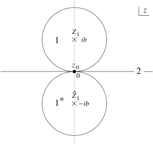
Fig. 18: $z$ plane of the open-closed transition vertex $\langle U(2,1^{\mathrm{c}})|$.

References

- [1] For a review, J. Polchinski, “Tasi Lectures on D-Branes”, hep-th/9611050.
- [2] T. Banks, W. Fischler, S.H. Shenker and L. Susskind, Phys. Rev. D55 (1997), 5112.
- [3] N. Ishibashi, H. Kawai, Y. Kitazawa and A. Tsuchiya, Nucl. Phys. B498 (1997), 467.
- [4] K. Hashimoto and H. Hata, Phys. Rev. D56 (1997), 5179.
- [5] B. Zwiebach, “Oriented Open-Closed String Theory Revisited”, hep-th/9705241.
- [6] M.B. Green and J.H. Schwarz, Phys. Lett. 151B (1985), 21.
- [7] H. Itoyama and P. Moxhay, Nucl. Phys. B293 (1987), 685.
- [8] M.R. Dougras and B. Grinstein, Phys. Lett. 183B (1987), 52.
- [9] C. Wendt, Nucl. Phys. B314 (1989), 209.
- [10] T. Kugo and H. Terao, Phys. Lett. 208B (1988), 416.
- [11] Y. Saitoh and Y. Tanii, Nucl. Phys. B325 (1989), 161.
- [12] Y. Saitoh and Y. Tanii, Nucl. Phys. B331 (1990), 744.
- [13] K. Kikkawa and S. Sawada, Nucl. Phys. B335 (1990), 677.
- [14] T. Kugo and T. Takahashi, in preparation.
- [15] C.G. Callan, C. Lovelace, C.R. Nappi and S.A. Yost, Nucl. Phys. B288 (1987), 525.
- [16] A. LeClair, M.E. Peskin and C.R. Preitschopf, Nucl. Phys. B317 (1989), 411.
- [17] H. Kunitomo and K. Suehiro, Nucl. Phys. B289 (1987), 157.
- [18] H. Hata, K. Itoh, T. Kugo, H. Kunitomo and K. Ogawa Phys. Rev. D34 (1986), 2360.
- [19] H. Hata, K. Itoh, T. Kugo, H. Kunitomo and K. Ogawa Phys. Rev. D35 (1987), 1318.
- [20] T. Kugo and B. Zwiebach, Prog. Theor. Phys. 87 (1992), 801.
- [21] W. Siegel, Phys. Lett. 142B (1984), 276.
- [22] A. Neveu and P.C. West, Nucl. Phys. B293 (1987), 266.
- [23] S. Uehara, Phys. Lett. 190B (1987), 76.
- [24] T. Kugo, in Quantum Mechanics of Fundamental Systems 2, ed. by C. Teitelboim and J. Zanelli (Plenum Publishing Corporation, 1989).
- [25] L. Alvarez-Gaum, C. Gomez, G. Moore and C. Vafa, Nucl. Phys. B303 (1988), 411.
- [26] S.B. Giddings and E. Martinec, Nucl. Phys. B278 (1986), 91.
- [27] T. Kugo and K. Suehiro, Nucl. Phys. B337 (1990), 434.
- [28] J.A. Shapiro and C.B. Thorn, Phys. Rev. D36 (1987), 432.
- [29] H. Hata and M.M. Nojori, Phys. Rev. D36 (1987), 1193.
- [30] D. Friedam, E. Martinec and S. Shenker, Nucl. Phys. B271 (1986), 93.
- [31] J. Dai, R.G. Leigh and J. Polchinski, Mod. Phys. Lett. A4 (1989), 2073.
- [32] M. Kaku and K. Kikkawa, Phys. Rev. D10 (1974), 1823.
- [33] M.B. Green and J.H. Schwarz, Nucl. Phys. B243 (1984), 475.