Dirichlet Topological Defects

Abstract

We propose a class of field theories featuring solitonic solutions in which topological defects can end when they intersect other defects of equal or higher dimensionality. Such configurations may be termed “Dirichlet topological defects”, in analogy with the D-branes of string theory. Our discussion focuses on defects in scalar field theories with either gauge or global symmetries, in (3+1) dimensions; the types of defects considered include walls ending on walls, strings on walls, and strings on strings.

NSF-ITP/97-117 hep-th/9711099

CWRU-P16-97

I Introduction

It has long been appreciated that field theories with spontaneously broken symmetries often support topological defects — solitonic solutions whose stability is guaranteed by a topological conservation law. A variety of such defects can occur, depending on the pattern of symmetry breaking in the model. When a symmetry group $G$ is spontaneously broken to a subgroup $H$, the types of defects supported depend on the homotopy properties of the vacuum manifold, ${\cal M}=G/H$. In a $(d+1)$-dimensional spacetime, $p$-dimensional defects ($p<d$) exist if the homotopy group ${\pi_{d-p-1}}({\cal M})$ is nontrivial. Thus, in 3 spatial dimensions there will be planar defects (domain walls) if ${\pi_{0}}({\cal M})\neq 0$, line-like defects (cosmic strings) if ${\pi_{1}}({\cal M})\neq 0$, and pointlike defects (monopoles) if ${\pi_{2}}({\cal M})\neq 0$. (For reviews see [1].)

In addition to these basic defects, there are various composite solutions which combine two of the types, generally when a $(p-1)$-dimensional defect serves as the boundary of a $p$-dimensional defect. Consider, for example, a sequence of symmetry breakings in which a group $G$ is broken to $H\times{\bf Z}_{2}$ at some high scale, and subsequently to $H$ at some lower scale, where both $G$ and $H$ are connected and simply connected. Then ${\pi_{1}}[G/(H\times{\bf Z}_{2})]={\bf Z}_{2}$, and strings will be formed at the first phase transition. A closed loop in physical space around the string, parameterized by $x^{\mu}(\lambda)$ as $\lambda$ goes from $0$ to $1$, defines a closed loop in field space which can be written $\phi(\lambda)=g(\lambda)\phi_{0}$, where $\phi_{0}$ is the initial value of the field and $g(\lambda)$ is a path in the group $G$ such that $g(0)=1$. The group element $g(1)$ corresponds not to the identity in $G$, but to the non-identity element in the unbroken ${\bf Z}_{2}$ subgroup. When this group is broken after the second phase transition, the path $\phi(\lambda)$ no longer describes a closed loop in the vacuum manifold; rather, a domain wall must form with the string as its boundary [2]. Looked at another way, if we were unaware of the full symmetry group $G$, we would predict the appearance of topologically stable walls due to the breaking $H\times{\bf Z}_{2}\rightarrow H$; but in fact the presence of $G$ implies that these walls can end on cosmic strings. Indeed, such walls are unstable to the nucleation of holes bounded by string loops (although the timescale for such processes may be extraordinarily long). Similarly, models can be constructed [3] in which strings end on monopoles, and can decay via the nucleation of monopole-antimonopole pairs along their length. Finally, in some theories the evolution of one kind of defect can lead to the creation or destruction of another kind; examples include domain walls sweeping up monopoles [4] and collapsing textures nucleating monopoles or string loops [5].

In this paper we discuss configurations which are complementary to those mentioned above — solutions in which defects can end when they intersect other defects of equal or higher dimensionality, such as strings ending on domain walls. For such configurations, we term the defects on which other defects end “Dirichlet topological defects”, in analogy with the D-branes of string theory. The latter are extended objects on which fundamental strings can end [6, 7, 8, 9]. The models considered here are ordinary field theories, which support topological solitons which resemble these objects in fundamental string theory. (Dirichlet defects in this sense have been discussed previously: cosmic strings ending on domain walls can arise in supersymmetric Yang-Mills theories [10] as well as in grand unified models [4], while the well-known phenomenon of non-intercommuting cosmic strings provides an example of strings ending on strings.) We will focus on the case of defects in bosonic field theories in (3+1) dimensions; generalization to higher dimensions and theories with fermions is left to future work.

II Walls Ending on Walls

In any number of spatial dimensions, the simplest example of Dirichlet topological defects consists of codimension-one defects ending on other codimension-one defects: for $d=3$, domain walls ending on domain walls. This example provides a paradigm for the models considered in subsequent sections.

Walls arise upon the breakdown of discrete symmetries, and it is therefore unnecessary to introduce gauge fields into our model at this stage. To form the Dirichlet wall (or D-wall) we introduce a single real scalar $\phi$, invariant under a symmetry group ${\bf Z}_{2}^{(1)}$ which acts on $\phi$ via $\phi\rightarrow-\phi$. If the potential energy is minimized at $\phi=\pm v$, the wall solution interpolates from one domain with $\langle\phi\rangle=v$ to another with $\langle\phi\rangle=-v$. We next introduce another real scalar $\psi_{1}$, invariant under a distinct symmetry group ${\bf Z}_{2}^{(2)}$ which sends $\psi_{1}$ to $-\psi_{1}$. In order for $\psi_{1}$ to lead to “fundamental” walls which can end on the D-wall, we require that the potential be minimized at $\psi_{1}=\pm w$ when $\phi=v$, and $\psi_{1}=0$ when $\phi=-v$. Such a potential is not invariant under the original symmetry ${\bf Z}_{2}^{(1)}$ unless we include a third real scalar $\psi_{2}$ which exchanges roles with $\psi_{1}$ under the action of ${\bf Z}_{2}^{(1)}$. That is, we consider a complete symmetry group ${\bf Z}_{2}^{(1)}\times{\bf Z}_{2}^{(2)}\times{\bf Z}_{2}^{(3)}$, with action

$${\bf Z}_{2}^{(1)}: \ \ \{\phi\rightarrow-\phi\ ,\ \psi_{1}\leftrightarrow\psi_{2}\}\ ,$$ (1)

$${\bf Z}_{2}^{(2)}: \ \ \psi_{1}\rightarrow-\psi_{1}\ ,$$ (2)

$${\bf Z}_{2}^{(3)}: \ \ \psi_{2}\rightarrow-\psi_{2}\ .$$ (3)

Such a symmetry allows for $\psi_{1}$-walls when $\langle\phi\rangle=v$ and $\psi_{2}$-walls when $\langle\phi\rangle=-v$; each can end on the Dirichlet walls where $\phi$ changes values.

Given the three scalar fields $\{\phi,\psi_{1},\psi_{2}\}$, a complete set of nonderivative interactions of no higher than fourth order which are consistent with these symmetries includes $\phi^{2}$, $\phi^{4}$, $(\psi_{1}^{2}+\psi_{2}^{2})$, $(\psi_{1}^{4}+\psi_{2}^{4})$, $\psi_{1}^{2}\psi_{2}^{2}$, $\phi^{2}(\psi_{1}^{2}+\psi_{2}^{2})$, and $\phi(\psi_{1}^{2}-\psi_{2}^{2})$. It is convenient to write the most general potential constructed from these terms in the form

$$V(\phi,\psi_{1},\psi_{2}) = \lambda_{\phi}(\phi^{2}-\widetilde{v}^{2})^{2}+\lambda_{\psi}\left[\psi_{1}^{2}+\psi_{2}^{2}-\widetilde{w}^{2}+g(\phi^{2}-\widetilde{v}^{2})\right]^{2}$$ (5)

$$\quad{}+h\psi_{1}^{2}\psi_{2}^{2}-\mu\phi(\psi_{1}^{2}-\psi_{2}^{2})\ .$$

We consider the parameter space in which $\lambda_{\phi}$, $\lambda_{\psi}$, $h$, $\widetilde{v}^{2}$ and $\widetilde{w}^{2}$ are all positive. The sign of $g$ is left unspecified, and we may take $\mu\geq 0$ without loss of generality (as a change in sign of $\mu$ is equivalent to a field redefinition interchanging $\psi_{1}$ and $\psi_{2}$). At $\mu=0$, the potential is the sum of three non-negative terms which may be simultaneously set to zero. It is therefore easy to see that there exist eight vacua, in which $\phi=\pm\widetilde{v}$ and $(\psi_{1},\psi_{2})$ are either $(\pm\widetilde{w},0)$ or $(0,\pm\widetilde{w})$. As $\mu$ is increased to positive values, this degeneracy is broken, and it becomes energetically favorable (for example) to have $|\psi_{1}|=w=\widetilde{w}+{\cal O}(\mu)$ and $|\psi_{2}|=0$ when $\phi=v=\widetilde{v}+{\cal O}(\mu)$.

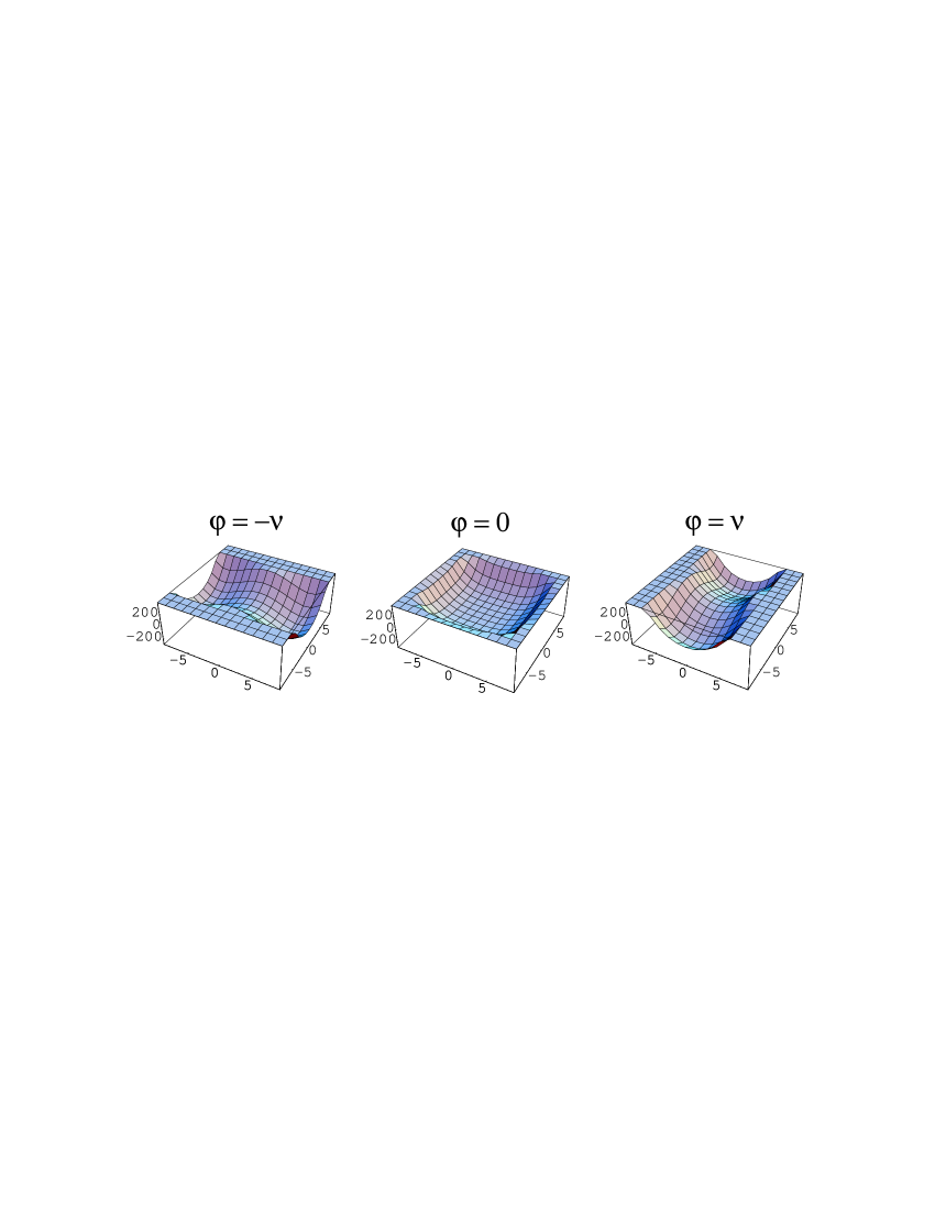
FIG. 1.: Shape of the potential as a function of $\psi_{1}$ (right horizontal axis) and $\psi_{2}$ (left horizontal axis), for three different values of $\phi$. When $\phi=v$, $\langle\psi_{1}\rangle=\pm w$ and $\langle\psi_{2}\rangle=0$, while when $\phi=-v$, $\langle\psi_{1}\rangle=0$ and $\langle\psi_{2}\rangle=\pm w$.

The potential in the vicinity of its minima is plotted in Fig. 1. There are four vacua of zero energy, of the form $\{\phi=v,\psi_{1}=\pm w,\psi_{2}=0\}$ and $\{\phi=-v,\psi_{1}=0,\psi_{2}=\pm w\}$. The vacuum expectation value (vev) $\langle|\phi|\rangle=v$ solves a cubic equation

$$8\lambda_{\phi}\lambda_{\psi}v^{3}-6\lambda_{\psi}g\mu v^{2}-(8\lambda_{\phi}\lambda_{\psi}\widetilde{v}^{2}+\mu^{2})v-2\lambda(g\widetilde{v}^{2}+\widetilde{w}^{2})\mu=0\ .$$ (6)

The correct root of this equation is the one which reduces to $\widetilde{v}$ at $\mu=0$. The vev $w$ is given in terms of $v$ by

$$w=\left(\widetilde{w}^{2}+g(\widetilde{v}^{2}-v^{2})-{\mu v\over{2\lambda_{\psi}}}\right)^{1/2}\ .$$ (7)

In any of these vacua, the original ${\bf Z}_{2}\times{\bf Z}_{2}\times{\bf Z}_{2}$ is broken to a single ${\bf Z}_{2}$ and the vacuum manifold is therefore ${\cal M}=({\bf Z}_{2}\times{\bf Z}_{2}\times{\bf Z}_{2})/{\bf Z}_{2}={\bf Z}_{2}\times{\bf Z}_{2}$. Starting from a single vacuum we can visit three different vacua, two of which are associated with Dirichlet walls of equal energy, and the third of which is associated with a fundamental wall.

The energies of the two types of wall are complicated functions of the parameters in the potential. However, there is a simple argument that provides an upper limit on the energy density of the fundamental wall in comparison to the D-wall:

$$E_{F}\leq 2E_{D}\ .$$ (8)

To see this, consider the energy of the fundamental wall as a functional of the wall profile. This is determined by the values of $\phi(x)$, $\psi_{1}(x)$ and $\psi_{2}(x)$ as $x$ takes values from $x_{1}$, where the fields are in (for example) the vacuum $\{\phi=v,\psi_{1}=w,\psi_{2}=0\}$, to $x_{2}$ where the fields are in the vacuum $\{\phi=v,\psi_{1}=-w,\psi_{2}=0\}$. This energy (per unit area) is given by

$$E_{F}=\int_{x_{1}}^{x_{2}}\left[{1\over 2}(\nabla\phi)^{2}+{1\over 2}(\nabla\psi_{1})^{2}+{1\over 2}(\nabla\psi_{2})^{2}+V(\phi,\psi_{1},\psi_{2})\right]\,dx\ .$$ (9)

The stable wall configuration is that which minimizes this energy. However, there are paths in field space which go through the intermediate point $\{\phi=-v,\psi_{1}=0,\psi_{2}=w\}$ and thus correspond to configurations representing two parallel D-walls. There may be (and typically will be) configurations with lower energy than this one, so the energy of the fundamental walls is bounded above by the energy of two D-walls.

It would appear to be very difficult to find exact solutions representing a fundamental wall ending on a D-wall. Not only do the configurations of the isolated walls involve the interactions of all three fields, but the D-wall is not expected to be smooth at the point where it is intersected by a fundamental wall; the tension from the latter will pull the D-wall into a cusp configuration. However, it may be possible to find solutions to an effective world-volume theory of the walls, and work in this direction has been undertaken for the case of D-branes in fundamental string theory [11].

III Strings Ending on Walls

The case of strings ending on D-walls in three spatial dimensions is an immediate generalization of the previous example. Strings arise most simply from the breakdown of ${\rm U}(1)$ symmetries; we therefore promote the real scalars $\psi_{1}$ and $\psi_{2}$ to complex fields $\psi_{i}=\rho_{i}e^{i\theta_{i}}$, and the symmetries acting on them to ${\rm U}(1)$’s, leaving the discrete ${\bf Z}_{2}$ (which breaks to give the D-walls) unchanged. The complete set of symmetries is therefore

$${\bf Z}_{2}: \{\phi\rightarrow-\phi\ ,\ \psi_{1}\leftrightarrow\psi_{2}\}\ ,$$ (10)

$${{\rm U}(1)}_{1}: \psi_{1}\rightarrow e^{-i\omega_{1}}\psi_{1}\ ,$$ (11)

$${{\rm U}(1)}_{2}: \psi_{2}\rightarrow e^{-i\omega_{2}}\psi_{2}\ .$$ (12)

The two ${\rm U}(1)$’s may be taken to be either global or gauge symmetries. In the latter case, $\omega_{1}$ and $\omega_{2}$ are functions of spacetime, and there are two gauge fields $A_{\mu}^{(1)}$, $A_{\mu}^{(2)}$, with the usual transformation properties

$$A_{\mu}^{(i)}\rightarrow A_{\mu}^{(i)}+\partial_{\mu}\omega_{i}$$ (13)

and associated covariant derivatives

$$D_{\mu}\psi_{i}=\partial_{\mu}\psi_{i}+iA_{\mu}^{(i)}\psi_{i}\ .$$ (14)

Since the real scalar $\phi$ is uncharged under both ${\rm U}(1)$’s, the kinetic term for $\phi$ is given in terms of ordinary partial derivatives.

The appropriate potential is now

$$V(\phi,\psi_{1},\psi_{2}) = \lambda_{\phi}(\phi^{2}-\widetilde{v}^{2})^{2}+\lambda_{\psi}\left[|\psi_{1}|^{2}+|\psi_{2}|^{2}-\widetilde{w}^{2}+g(\phi^{2}-\widetilde{v}^{2})\right]^{2}$$ (16)

$$\quad{}+h|\psi_{1}|^{2}|\psi_{2}|^{2}-\mu\phi(|\psi_{1}|^{2}-|\psi_{2}|^{2})\ .$$

In the vacuum the real scalar $\phi$ takes the vev $\pm v$ and there may exist domain walls separating these two values. When $\langle\phi\rangle=+v$, the vacuum has $|\psi_{1}|=v$ and $\psi_{2}=0$, while when $\langle\phi\rangle=-v$ the vacuum has $|\psi_{2}|=v$ and $\psi_{1}=0$. The values of $v$ and $w$ are as in the last section.

In this model, therefore, the unbroken symmetry group in the true vacuum is ${\rm U}(1)$, and the vacuum manifold is ${\cal M}=[{\rm U}(1)\times{\rm U}(1)\times{\bf Z}_{2}]/{\rm U}(1)=S^{1}\times{\bf Z}_{2}$, admitting walls and strings. When $\langle\phi\rangle=+v$, the complex field $\psi_{1}$ can form cosmic strings with winding number $n$, around which $\theta_{1}$ will change by $2\pi n$. Such a string ends if it intersects a D-wall, since $\langle\psi_{1}\rangle=0$ on the other side. Analogous statements hold for the $\psi_{2}$ field when $\langle\phi\rangle=-v$.

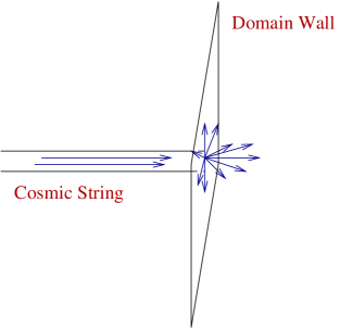
FIG. 2.: A cosmic string ends on a Dirichlet domain wall in 3 spatial dimensions. The arrows denote the magnetic flux.

In the core of a string the corresponding ${\rm U}(1)$ symmetry is restored. In the gauge case, therefore, the gauge bosons associated with, for example, ${{\rm U}(1)}_{1}$ are massless both in the core of a $\psi_{1}$-string on the $\langle\phi\rangle=v$ side of the D-wall, and anywhere on the $\langle\phi\rangle=-v$ side of the D-wall. As usual, outside the $\psi_{1}$-string the gauge field is pure gauge, such that it cancels the gradient energy of the scalars by enforcing the vanishing of the covariant derivative (14). The gauge field is thus given by $A_{\mu}^{(1)}=-\partial_{\mu}\theta_{1}$. Consequently, there is magnetic flux through the string (which we take to have winding number $n$), given by $\Phi^{(1)}=-n\pi$. This flux flows through the string until it hits the wall; on the other side of the wall the symmetry is unbroken everywhere, and the magnetic field describes a monopole configuration emanating from the point where the string intersects the wall. We sketch such a configuration in Fig. 2.

Configurations of the this type, with strings ending on walls, have recently been discussed in the context of supersymmetric QCD [10]. There, the string consists of non-Abelian flux, and the wall separates different chiral vacua, with shifted values of the QCD $\theta$-parameter. The intersections of strings and domain walls can be thought of as quarks. The structures of these QCD configurations and the scalar field models discussed here are obviously very similar, and the relationship between them deserves further investigation. (One difference is that the flux in the strings considered in [10] does not propagate freely on the other side of the wall, as the symmetry is still broken there; rather, it is confined to the wall itself. It should not be difficult to extend models of the type considered in this paper to include such situations.) They have also been shown to exist in certain grand unified theories [4]. Here, conventional GUT monopoles can become bound to domain walls, and the monopoles will become connected by strings if the color gauge group ${\rm SU}(3)$ is broken to ${\bf Z}_{3}$.

IV Strings and strings

A number of theories in which a cosmic string can end on another string can be found in the literature. Generally speaking, three-string vertices can arise whenever the strings are associated with elements $a$, $b$, and $c$ of ${\pi_{1}}({\cal M})$, such that $abc=1$. Configurations of this type play an important role in models where ${\pi_{1}}({\cal M})$ is non-Abelian, and may have interesting cosmological consequences (see for example [12]).

Nevertheless, it is interesting to consider theories of strings ending on strings which more closely resemble those of the last two sections; that is, with two types of strings, one of which may be thought of as fundamental and the other as Dirichlet (characterized by the fact that fundamental strings can end on Dirichlet strings but not vice-versa). As we shall see, the construction of such models closely parallels that of the theories with Dirichlet walls.

We once again consider three fields $\phi$, $\psi_{1}$, and $\psi_{2}$, now with all three being complex scalars, for a total of six real degrees of freedom. We impose two ${\rm U}(1)$ symmetries, under which the fields have the following charges:

$$\matrix{&&\underline{{{\rm U}(1)}_{1}}&\underline{{{\rm U}(1)}_{2}}\cr\cr\phi&&2&0\cr\psi_{1}&&1&1\cr\psi_{2}&&1&-1\cr}$$ (17)

We also include a ${\bf Z}_{2}$ with action

$$\psi_{1}\leftrightarrow\psi_{2}\ .$$ (18)

A general potential may be written in a form reminiscent of (but not identical to) our previous examples:

$$V(\phi,\psi_{1},\psi_{2}) = \lambda_{\phi}\left(|\phi|^{2}-\widetilde{v}^{2}\right)^{2}+\lambda_{\psi}\left[|\psi_{1}|^{2}+|\psi_{2}|^{2}-\widetilde{w}^{2}+g(|\phi|^{2}-\widetilde{v}^{2})\right]^{2}$$ (20)

$$\quad+h\left(|\psi_{1}|^{2}-|\psi_{2}|^{2}\right)^{2}-\mu\left(\psi_{1}^{*}\psi_{2}^{*}\phi+\psi_{1}\psi_{2}\phi^{*}\right)\ .$$

We describe the complex scalars in terms of their moduli and phases as $\phi=\rho_{\phi}e^{i\theta_{\phi}}$, $\psi_{1}=\rho_{1}e^{i\theta_{1}}$, $\psi_{2}=\rho_{2}e^{i\theta_{2}}$. As before, for $\mu=0$ the potential is the sum of three non-negative terms, which can be simultaneously set to zero by setting $\langle\rho_{\phi}\rangle=\widetilde{v}$ and $\langle\rho_{1}\rangle=\langle\rho_{2}\rangle=\widetilde{w}$. Turning on a small positive $\mu$ introduces a constraint on the phases: $\langle\theta_{\phi}\rangle=\langle\theta_{1}\rangle+\langle\theta_{2}\rangle$. The unbroken subgroup is ${\bf Z}_{2}$, which in general is a combination of the original ${\bf Z}_{2}$ and a ${{\rm U}(1)}_{2}$ transformation. The vacuum manifold is therefore a torus, ${\cal M}=[{\rm U}(1)\times{\rm U}(1)\times{\bf Z}_{2}]/{\bf Z}_{2}=S^{1}\times S^{1}$, which may be parameterized by the angles $\theta_{1}$ and $\theta_{2}$, determining the remaining angle $\theta_{\phi}$.

Strings are characterized by elements of ${\pi_{1}}(S^{1}\times S^{1})={\bf Z}\times{\bf Z}$. We can take the two generators $(1,0)$ and $(0,1)$ to be given by paths from $\theta_{i}=0$ to $\theta_{i}=2\pi$, for $i=1,2$ respectively. (In each case $\theta_{\phi}$ also ranges from $0$ to $2\pi$.) Due to the ${\bf Z}_{2}$ symmetry, strings corresponding to either of the two generators have equal tensions. A string corresponding to $(1,-1)$, although it may be thought of as a superposition of strings with charges $(1,0)$ and $(0,-1)$, can have a lower energy than the two separately (since $\rho_{1}$ equals $\rho_{2}$, and thus the term in the potential of the form $h[|\psi_{1}|^{2}-|\psi_{2}|^{2}]$ vanishes) and therefore be stable against decay; strings of this type are the fundamental strings, while those with charges $(1,0)$ or $(0,1)$ are the D-strings.

The gauge transformations in ${\rm U}(1)_{1}$ and ${\rm U}(1)_{2}$ can be written in terms of functions $\omega_{1}(x^{\mu})$ and $\omega_{2}(x^{\mu})$ as

$$\left(\matrix{\phi\cr\psi_{1}\cr\psi_{2}\cr}\right)\rightarrow\left(\matrix{e^{-2i\omega_{1}}\phi\cr e^{-i(\omega_{1}+\omega_{2})}\psi_{1}\cr e^{-i(\omega_{1}-\omega_{2})}\psi_{2}\cr}\right)\ .$$ (21)

In the core of the $(1,-1)$ string, we have $\langle\phi\rangle=v$, $\langle\psi_{1}\rangle=\langle\psi_{2}\rangle=0$, and the ${\rm U}(1)_{2}$ symmetry (transformations with $\omega_{1}=0$) is restored. In a $(1,0)$ string there is an unbroken ${\rm U}(1)$ parameterized by $\omega_{1}=\omega_{2}$, and in a $(0,1)$ string there is an unbroken ${\rm U}(1)$ parameterized by $\omega_{1}=-\omega_{2}$.

Outside the string cores, the gauge fields are pure gauge such that they cancel the gradient energy in the scalars. This means they enforce the vanishing of the covariant derivatives

$$D_{\mu}\phi = \partial_{\mu}\phi+2iA_{\mu}^{(1)}\phi\ ,$$ (22)

$$D_{\mu}\psi_{1} = \partial_{\mu}\psi_{1}+iA_{\mu}^{(1)}\psi_{1}+iA_{\mu}^{(2)}\psi_{1}\ ,$$ (23)

$$D_{\mu}\psi_{2} = \partial_{\mu}\psi_{2}+iA_{\mu}^{(1)}\psi_{2}-iA_{\mu}^{(2)}\psi_{2}\ .$$ (24)

The gauge fields are thus given by

$$A_{\mu}^{(1)} = {1\over{2}}\partial_{\mu}(\theta_{1}+\theta_{2})={1\over{2}}\partial_{\mu}\theta_{\phi}\ ,$$ (25)

$$A_{\mu}^{(2)} = {1\over{2}}\partial_{\mu}(\theta_{1}-\theta_{2})\ .$$ (26)

Consequently, the magnetic fluxes through a string with winding number $(n,m)$ are

$$\Phi^{(1)}(n,m) = (n+m)\pi\ ,$$ (27)

$$\Phi^{(2)}(n,m) = (n-m)\pi\ .$$ (28)

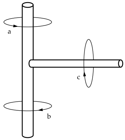
FIG. 3.: A fundamental cosmic string ends on a Dirichlet string. The homotopy classes of the indicated loops in ${\pi_{1}}(S^{1}\times S^{1})={\bf Z}\times{\bf Z}$ are $[a]=(1,0)$, $[b]=(0,-1)$, and $[c]=(1,-1)$.

In Fig. 3 we show a configuration with a fundamental string ending on a D-string. Around the latter, the phase of $\phi$ changes by $2\pi$; above the intersection point it is accompanied by the phase of $\psi_{1}$ ($\theta_{1}=\theta_{\phi}$, $\theta_{2}=0$), while below the intersection point it is accompanied by the phase of $\psi_{2}$ ($\theta_{2}=\theta_{\phi}$, $\theta_{1}=0$). The fundamental string is topologically equivalent to the superposition of the two segments of the D-string (as it must be, since the loops $a$ and $b$ together are topologically equivalent to loop $c$); around it the phases $\theta_{1}$ and $\theta_{2}$ change by $2\pi$, while $\theta_{\phi}$ is constant. It is easy to verify that the configuration shown conserves flux: through $a$ we have $\Phi^{(1)}=\pi$, $\Phi^{(2)}=\pi$; through $b$ we have $\Phi^{(1)}=\pi$, $\Phi^{(2)}=-\pi$; and through $c$ we have $\Phi^{(1)}=0$, $\Phi^{(2)}=2\pi$.

V Conclusions

We have described a class of topological defects in classical field theories in (3+1) dimensions, consisting of Dirichlet defects on which fundamental defects of lower dimension can terminate. While the search for models supporting these configurations is inspired by the appearance of D-branes in string theory, there are important differences between the two sets of objects. In all of the theories we consider, the basic degrees of freedom are scalar fields and gauge fields, out of which all of the higher-dimensional objects are constructed. Our theories do not include the effects of gravity, and are not supersymmetric (although there are no obstacles to the appropriate generalizations). Furthermore, the specific dependence of D-brane energy on the string coupling constant is not a feature of our models, and the Ramond-Ramond gauge fields to which D-branes couple are absent. Nevertheless, it may be interesting to compare the dynamical behavior of Dirichlet defects to that of D-branes in string theory, and search for models in which the similarities between the two systems are even stronger.

One obvious direction in which to generalize the models considered here is to consider $q$-dimensional defects ending on $p$-dimensional D-defects in $d$ spatial dimensions. (There are a variety of such objects in string theory and M-theory, with configurations governed by charge conservation [13].) A number of interesting issues arise in this case, especially for gauge symmetries. In three spatial dimensions, domain walls, strings and monopoles all have finite energy (per unit volume) if they arise from the spontaneous breakdown of gauge symmetries, while strings and monopoles in theories with global symmetries have divergent energies. More generally, gauge defects of codimension greater than three have divergent energies, as have global defects of codimension greater than one [14]. Although the divergence of the energy is an important feature of such configurations, it does not render them unphysical; certainly there is no obstacle in principle, for example, to the existence of global strings in (3+1) dimensions. More importantly, to make topological defects of dimension $q$ in $d$ spatial dimensions requires that ${\pi_{d-q-1}}({\cal M})$ be nontrivial, for example by breaking ${\rm SO}(d-p)$ to ${\rm SO}(d-p-1)$ (for which ${\cal M}=S^{d-p-1}$). In such a model, the unbroken symmetry group ${\rm SO}(d-p-1)$ is non-Abelian for $p\leq d-4$; we then expect the low-energy gauge theory to be strongly coupled, and the resulting defects to be confined.

Back in (3+1) dimensions, there are a number of issues remaining to be addressed. As mentioned, the models we have constructed are purely bosonic, and it would be interesting to consider supersymmetric versions (as has been done for non-hybrid defects [15]), as well as to determine whether Dirichlet defects could arise in realistic particle physics models. Finally, as with any species of topological defect, it is also natural to ask what the cosmological consequences of the formation of these objects in the early universe might be.

REFERENCES

- [1] A. Vilenkin and E.P.S. Shellard, Cosmic Strings and Other Topological Defects, Cambridge University Press (1994); M.B. Hindmarsh and T.W.B. Kibble, Rept. Prog. Phys. 58, 477 (1995), hep-ph/9411342.
- [2] T.W.B. Kibble, G. Lazarides, and G. Shafi, Phys. Rev. D 26, 435 (1982).
- [3] F.A. Bais, Phys. Lett. 98B, 437 (1981); A. Vilenkin, Nucl. Phys. B196, 240 (1982); M.B. Hindmarsh and T.W.B. Kibble, Phys. Rev. Lett. 55, 2398 (1985).
- [4] G. Dvali, H. Liu, and T. Vachaspati, “Sweeping Away the Monopole Problem”, hep-ph/9710301.
- [5] I. Chuang, R. Durrer, N. Turok, and B. Yurke, Science 251, 1336 (1991); A. Sornborger, S.M. Carroll, and T. Pyne, Phys. Rev. D 55, 6454 (1997), hep-ph/9701351.
- [6] P. Horava, Nucl. Phys. B327, 461 (1989); Phys. Lett. B231 351 (1989).
- [7] J. Dai, R.G. Leigh, and J. Polchinski, Mod. Phys. Lett. A4, 2073 (1989).
- [8] J. Polchinski, Phys. Rev. Lett. 75, 4724 (1995), hep-th/9510017.
- [9] J. Polchinski, S. Chaudhuri, and C.V. Johnson, “Notes on D-branes”, hep-th/9602052; J. Polchinski, “TASI Lectures on D-branes”, hep-th/9611050.
- [10] E. Witten, “Membranes and the Dynamics of QCD”, hep-th/9706109; S.-J. Rey, to appear.
- [11] E. Witten, Nucl. Phys. B500, 3 (1997), hep-th/9703166; C.G. Callan and J.M. Maldecena, “Brane Dynamics from the Born-Infeld Action”, hep-th/9708147; G.W. Gibbons, “Born-Infeld Particles and Dirichlet -Branes”, hep-th/9709027; P.S. Howe, N.D. Lambert, and P.C. West, “The Selfdual String Soliton”, hep-th/9709014; A. Hashimoto, “The Shape of Branes Pulled by Strings”, hep-th/9711097.
- [12] V. Poénaru and G. Toulouse, J. de Physique 8, 887 (1977); N.D. Mermin, Rev. Mod. Phys. 51, 591 (1979); T.W.B. Kibble, Phys. Rep. 67, 183 (1980); J.L. Chkareuli, Phys. Lett. B272, 207 (1991); G. Dvali and G. Senjanovic, Phys. Rev. Lett. 72, 9 (1994); D. Spergel and U.-L. Pen, “Cosmology in a String-Dominated Universe”, astro-ph/9611198; P. McGraw, “Evolution of a Non-Abelian Cosmic String Network”, astro-ph/9706182.
- [13] A. Strominger, Phys. Lett. B383, 44 (1996), hep-th/9512059.
- [14] S. Coleman, Aspects of Symmetry, Cambridge University Press, 1985.
- [15] S.C. Davis, A.-C. Davis and M. Trodden, Phys. Lett. B405, 257 (1997); “Cosmic Strings, Zero Modes and SUSY Breaking in Nonabelian Gauge Theories”, hep-ph/9711313; J.R. Morris, Phys. Rev. D52, 1096 (1995); Phys. Rev. D53, 2078 (1996); Phys. Rev. D56, 2378 (1997).