A Technique for Calculating Quantum Corrections to Solitons

Abstract

We present a numerical scheme for calculating the first quantum corrections to the properties of static solitons. The technique is applicable to solitons of arbitrary shape, and may be used in 3+1 dimensions for multiskyrmions or other complicated solitons. We report on a test computation in 1+1 dimensions, where we accurately reproduce the analytical result with minimal numerical effort.

I Introduction

The quantum fate of static solitons has long been studied, and beautiful results have emerged in exactly solvable two dimensional field theories. In higher dimensions, very little is known except in certain very special supersymmetric theories, or in situations of spherical symmetry. In many theories, the quantum properties of the soliton-bearing sector are interesting, but beyond the reach of current calculations. One example of such a theory is the chiral model of nuclear physics, the solitonic sector of which describes nucleons and nuclei[2]. It is clear that quantum effects must be included if the theory is to match real nuclei, but hitherto only a very limited ‘collective coordinate’ quantization has been possible. There are many other 3+1 dimensional field theories with topological solitons, for example those bearing magnetic monopoles and vortex strings. It would be very useful to develop techniques to study quantum corrections to these solitons in both supersymmetric and non-supersymmetric contexts.

The quantum corrections to a soliton’s classical properties may be expressed as an expansion in a dimensionless parameter, some power of the coupling constant, multiplied by Planck’s constant $\hbar$. At weak coupling, the corrections are small and may be calculated perturbatively in this small parameter. In this paper we outline a straightforward method for numerically computing the first quantum corrections, including all fluctuations about a static soliton, to first order in $\hbar$. In particular, we present a method for calculating the quantum correction to the soliton mass, although the technique is easily generalized to other quantum corrections. We apply the method to a simple two dimensional theory where the exact expression is known, and show that it is reproduced numerically with little computational cost. We also discuss the extension of the method to analogous calculations in four dimensions.

There exist a set of standard techniques for calculating the quantum corrections to the mass, moments, and other properties of solitons [6]. The techniques usually used require knowledge of the phase shifts associated with every possible meson scattering from the soliton. However in many cases of interest, for example multi-Skyrmions [4], the soliton field is not spherically symmetric and the necessary information would be extremely difficult to extract.

In this paper we present a different approach, based upon quantizing the soliton in a finite box, which provides an infrared regulator and reduces the number of modes to be quantised to a discrete set. Our method centers upon a formula for the first quantum mass corrections due to Cahill et al.[8], which automatically removes the worst divergences. The quantum correction to the soliton mass is given as a trace over a complete set of modes. We compute this trace by summing first over the lowest normal modes of the soliton, and then over a plane wave basis up to a finite cutoff. The contribution of modes beyond this cutoff is included analytically using a derivative expansion. As we shall show, one per cent accuracy in the mass correction is achievable with very modest computational resources. We point toward the application of this technique to more interesting problems, where it appears feasible to calculate the quantum corrections for multisolitons in the Skyrme model [3], and other 3+1 dimensional theories.

II Fluctuations about classical solitons

We would like to quantize small fluctuations about some stable, static classical soliton. The field’s dynamics are determined by a Lagrangian, ${\cal L}(\phi,\partial\phi)$, which gives classical equations of motion

$$\partial_{t}^{2}\phi^{a}=F^{a}(\phi,\partial\phi,\partial^{2}\phi)\ .$$ (1)

with the soliton  $\phi^{a}_{\rm st}(\mbox{\boldmath$x$})$ as a time-independent solution. The soliton is a smooth, localized ‘lump’ in space, surrounded by a vacuum of constant field. The field $\phi^{a}(\mbox{\boldmath$x$},t)$ may be represented as the sum of the (c-number) classical soliton, $\phi_{\rm st}(\mbox{\boldmath$x$})$, plus a quantum correction $\epsilon(\mbox{\boldmath$x$},t)$ which is an operator obeying canonical commutation relations. We work to first order in $\hbar$, which amounts to keeping terms up to second order in $\epsilon(\mbox{\boldmath$x$},t)$ in the the Hamiltonian.

In this approximation, the quantum mechanical Hamiltonian is

$$H_{T}=E_{\rm cl}+:\int d^{d}x\ {\cal H}_{2}(\pi^{a},\epsilon^{a},\partial_{i}\epsilon^{a},x):\ ,$$ (2)

where $E_{\rm cl}=\int d^{d}xV(\phi_{\rm st},\partial\phi_{\rm st})$ is the classical soliton mass, and ${\cal H}_{2}$ quadratic in $\epsilon$ and its conjugate momentum $\pi$. Normal ordering is with respect to the trivial vacuum normal modes for $\epsilon$, the free mesons, so the Hamiltonian is zero in the soliton-free vacuum.

We may express $\epsilon^{a}(\mbox{\boldmath$x$},t)$ in terms of normal modes about the classical soliton. It obeys a linear equation

$$\partial_{t}^{2}\epsilon^{a}=-H^{2}_{ab}\epsilon^{b}$$ (3)

with $H^{2}_{ab}$ a positive semi-definite differential operator depending on the soliton solution. The eigenvalues of $H^{2}$ are the frequencies squared $\omega_{n}^{2}$ of the normal modes about the soliton. We then write

$$\epsilon^{a}(\mbox{\boldmath$x$},t)=\sum_{n}\left[{e^{-i\omega_{n}t}\over\sqrt{2\omega_{n}}}a_{n}\epsilon^{a}_{n}(\mbox{\boldmath$x$})+{\rm c.c.}\right]\ ,$$ (4)

where $\epsilon^{a}_{n}(\mbox{\boldmath$x$})$ is the $n$th classical normal mode, and $a_{n}$ is the associated annihilation operator. In terms of these normal mode operators, the Hamiltonian is

$$H_{T}=E_{\rm cl}+:\sum_{n}\omega_{n}a_{n}^{\dagger}a_{n}:\ .$$ (5)

where normal ordering is with respect to the trivial soliton-free vacuum. The ground state of this Hamiltonian in the presence of a soliton can be computed by normal ordering the second term with respect to the soliton normal modes. To do so, write the operators $a_{n}^{\dagger},a_{n}$, in terms of $a^{a\dagger}(\mbox{\boldmath$k$}),a^{a}(\mbox{\boldmath$k$})$, the creation and annihilation operators for fluctuations about the soliton-free vacuum.

$$a_{n}^{\dagger}={1\over 2}\sum_{k}\left[\tilde{\epsilon}^{a}_{n}(-\mbox{\boldmath$k$})a^{a\dagger}(\mbox{\boldmath$k$})\left(\sqrt{\omega_{n}\over\omega_{k}}+\sqrt{\omega_{k}\over\omega_{n}}\right)+\tilde{\epsilon}^{a}_{n}(\mbox{\boldmath$k$})a^{a}(\mbox{\boldmath$k$})\left(\sqrt{\omega_{n}\over\omega_{k}}-\sqrt{\omega_{k}\over\omega_{n}}\right)\right]\ ,$$ (6)

where $\omega_{k}=\sqrt{k^{2}+m^{2}}$ are the frequencies of elementary meson excitations. Applying this identity, one finds

$$\omega_{n}a^{\dagger}_{n}a_{n} = :\omega_{n}a^{\dagger}_{n}a_{n}:+{1\over 4}\sum_{k}\tilde{\epsilon}_{n}^{a}(\mbox{\boldmath$k$})\tilde{\epsilon}_{n}^{a}(-\mbox{\boldmath$k$}){(\omega_{n}-\omega_{k})^{2}\over\omega_{k}}$$ (7)

$$= :\omega_{n}a^{\dagger}_{n}a_{n}:+{1\over 4}\left\langle n\biggr{|}{(H-H_{0})^{2}\over H_{0}}\biggr{|}n\right\rangle\ ,$$ (8)

where $H$ is the single particle Hamiltonian for fluctuations about the soliton, i.e., the positive square root of $H^{2}$, and $H_{0}$ is the single particle Hamiltonian for fluctuations about the soliton-free vacuum.

So, the total Hamiltonian may be written

$$H_{T}=E_{\rm cl}+\sum_{n}\omega_{n}a^{\dagger}_{n}a_{n}+\delta m,$$ (9)

where $\delta_{m}$, the quantum correction to the soliton mass, is

$$\delta m=-{1\over 4}{\rm Tr}\left[{(H-H_{0})^{2}\over H_{0}}\right],$$ (10)

a result obtained by Cahill, Comtet and Glauber [8]. The trace is taken over any complete set of states. In one dimension, (9) is finite and no further renormalization is needed. In three space dimensions it diverges logarithmically, and so requires regularization, which may be provided by inserting a factor $e^{-\epsilon H_{0}^{2}}$. The logarithmic divergence which results may then be subtracted with a local counterterm [13]. Nevertheless, the formula (10) is still very useful in three dimensions, as it has removed both the quartic and quadratic divergences.

To compute the trace (10) we need to be able to construct the three  terms $\langle\alpha|e^{-\epsilon H_{0}^{2}}H|\alpha\rangle$, $\langle\alpha|e^{-\epsilon H_{0}^{2}}H_{0}^{-1}H^{2}|\alpha\rangle$, and $\langle\alpha|e^{-\epsilon H_{0}^{2}}H_{0}|\alpha\rangle$, where the states  $|\alpha\rangle$ are the elements of some basis for field perturbations. A moments thought reveals that the last two terms are simple to compute, since we have an explicit form for the operator $H^{2}$, and the action $H_{0}$ on any perturbation is trivial (21). The difficulty lies with the first term, the trace of $H$ over its positive frequency subspace. This trouble arises because one does not have the $H$ operator in a calculationally useful form.

A The $H^{2}$ operator

In order to calculate the mass correction, (10), we need the $H^{2}$ operator, which can be extracted from the classical perturbation dynamics. To second order in $\epsilon^{a}$, the perturbation Lagrangian is

$${\cal L}(\epsilon,\partial\epsilon)=\partial_{t}\epsilon^{a}I_{ab}\partial_{t}\epsilon^{b}-\partial_{i}\epsilon^{a}\left(V_{ab;ij}\partial_{j}+W_{ab;i}\right)\epsilon^{b}-\epsilon^{a}M_{ab}\epsilon^{b}\ ,$$ (11)

where the tensors $I(\mbox{\boldmath$x$}),V(\mbox{\boldmath$x$}),W(\mbox{\boldmath$x$}),M(\mbox{\boldmath$x$})$ are functions of the static soliton fields. The classical time evolution of $\epsilon^{a}(\mbox{\boldmath$x$},t)$ is

$$\partial_{t}^{2}\epsilon^{a} = \left[I^{-1}\right]^{ab}\left(V_{bc;ij}\partial_{ij}+\partial_{i}V_{bc;ij}\partial_{j}+\partial_{i}W_{bc;i}-M_{bc}\right)\,\epsilon^{c}$$ (12)

$$= -H^{2}\circ\epsilon\ .$$ (13)

And so the classical equations of motion for the perturbation yield an operator, $H^{2}$, whose eigenvalues are the squares of the normal mode frequencies of perturbations about the soliton.

B Low normal modes of the soliton

We have $H^{2}$; unfortunately its positive square root $H$ cannot be easily represented. So, one cannot calculate all terms in the trace (10) directly. However, let us note several points. First, the main contribution in (10) comes from the lowest frequency normal modes of the soliton; these are the modes where the difference between the $\langle n|H|n\rangle$ and $\langle n|H_{0}|n\rangle$ are greatest. Indeed several authors, e.g. [9], [10], go so far as to include only the contribution of the soliton zero modes to the trace. This is not an accurate approximation, however it is important to accurately compute the contributions of the lowest modes. Second,  $H^{2}$ shares eigenvectors with $H$. So, although we cannot directly construct $H$, we can find its eigenvectors and eigenvalues if we can extract them from $H^{2}$. Finally, it is clear that very short wavelength modes should be accurately described by the WKB approximation - their contribution to the renormalized mass correction should be small, local and analytically calculable via a derivative expansion.

Our strategy is summarized in the following formula:

$${\rm Tr}\left[{\cal O}\right] = {\rm Tr}_{n}\left[{\cal O}\right]+{\rm Tr}_{{}_{k\leq k_{\rm max}}}\!\left[(1-P){\cal O}\right]+{\rm Tr}_{{}_{k>k_{\rm max}}}\!\left[(1-P){\cal O}\right]\ ,$$ (14)

$${\rm where}\qquad{\cal O} = H_{0}^{-1}(H-H_{0})^{2}\ .$$ (15)

Here $\{|n\rangle\}$ is a small set of precise, low frequency normal modes for the soliton, computed numerically as explained below, and used to take the first trace. The remaining part of the trace is computed using a simple plane wave basis $e^{i{\bf k.x}}$, corrected for overcounting using a projection operator $1-P$ with $P=\sum_{n}|n\rangle\langle n|$. The contribution from low momentum modes $k<k_{{\rm max}}$ is computed by straightforward matrix diagonalization. The final term from modes with $k>k_{{\rm max}}$ is computed analytically via a local derivative expansion as explained below.

The lowest frequency normal modes of $H^{2}$ may be extracted using the real-time method of [5], or by using $H^{2}$ to  drive a diffusion equation. The latter method has the advantage that for a limited set of modes the result converges more rapidly with integration time. For a fluctuation $|\epsilon\rangle$ about the static soliton, write

$$\partial_{\tau}|\epsilon\rangle=-H^{2}|\epsilon\rangle\ .$$ (16)

Now, create an initial perturbation $|\epsilon(0)\rangle$. This may be written in terms of eigenvectors $|n\rangle$ of $H^{2}$, with $H^{2}|n\rangle=\omega_{n}^{2}|n\rangle$.

$$|\epsilon(0)\rangle=\sum_{n}\epsilon_{n}|n\rangle\ ,$$ (17)

so the solution of the diffusion equation (16) is

$$|\epsilon(\tau)\rangle=\sum_{n}e^{-\omega_{n}^{2}\tau}\epsilon_{n}|n\rangle\ .$$ (18)

Starting in any state $|\epsilon\rangle$, and evolving it forward according to the diffusion equation (16), the resulting state rapidly becomes dominated by the lowest frequency mode.

To find the lowest frequency normal modes of $H$, one starts with an arbitrary perturbation field $|\epsilon\rangle$ and evolves it forward according to the diffusion equation, until the resulting field is an acceptably pure eigenvector of $H^{2}$. Call this eigenvector $|1\rangle$ and store it. Next, take another perturbation, $|\epsilon^{\prime}\rangle$, and project $|1\rangle$ out of it, and evolve it forward under the diffusion equation until one has another eigenvector of $H^{2}$. Orthonormalize this with respect to $|1\rangle$, and call it $|2\rangle$, and store it. And so on: in this way one builds up an archive spanning the lowest frequency normal modes of perturbations about the soliton. Individual perturbations in this archive will be a mixture of nearby normal modes of $H$, since evolving the diffusion equation forward a finite length of time only separates out modes with substantially different frequencies. However, once created, this archive of wavefunctions will span the space of the the lowest frequency normal modes of $H^{2}$, up to a cutoff frequency $\omega_{c}<\omega_{\max}$, the highest frequency probed. From this mixed archive of low normal modes, one can create a near-perfect archive by diagonalizing the matrix $\langle i|H^{2}|j\rangle$, creating a new archive of perturbations, out of linear combinations of the old ones. Any new perturbation field $|i^{\prime}\rangle$, will be a near machine-perfect eigenvector of $H^{2}$ if its frequency satisfies

$$e^{\left({\omega_{i}^{\prime}}^{2}-\omega_{\max}^{2}\right)T}\ll 1\ ,$$ (19)

where $T$ is the finite time the diffusion equation evolved forward. All but the highest handful of modes extracted in this fashion will be near-perfect; those remaining will be discarded before further calculation. In the example shown later, we kept only the 9 lowest frequency modes (including the zero mode) as our set $\{|n\rangle\}$ of near-perfect low modes.

The contribution of the near-perfect modes is easy to calculate, since

$$H^{2}|n\rangle=\omega_{n}^{2}|n\rangle\quad\Longrightarrow\quad H|n\rangle=\omega_{n}|n\rangle$$ (20)

and $H_{0}$ acts on any perturbation via

$$H_{0}|\epsilon\rangle=\sum_{k}\sqrt{k^{2}+m^{2}}|\mbox{\boldmath$k$}\rangle\langle\mbox{\boldmath$k$}|\epsilon\rangle\ .$$ (21)

(Here the basis $|\mbox{\boldmath$k$}\rangle$ is an abbreviation for all possible plane wave perturbations of the field; for several component fields it carries an internal space index as well as a wavevector.) And so, in the basis of normal modes of $H$, it is straightforward to get each term in the trace.

III Calculating the trace over all fluctuations

We wish to calculate the trace (10) over all modes, however it is not practical to compute all of them as above. Instead we proceed by supplementing our near-perfect eigenmodes with a trace over plane waves.

For the set of plane waves we simply construct the matrix

$$H^{2}_{kk^{\prime}}=\langle\mbox{\boldmath$k$}^{\prime}|H^{2}|\mbox{\boldmath$k$}\rangle$$ (22)

for all plane waves $\mbox{\boldmath$k$},\mbox{\boldmath$k$}^{\prime}$ satisfying $k\leq k_{\rm max}$. We then diagonalize this matrix:

$$H^{2}_{kk^{\prime}}={\cal O}^{\top}_{kd}\left[H^{2}_{D}\right]_{dd^{\prime}}{\cal O}_{d^{\prime}k^{\prime}}\ ,$$ (23)

where ${\cal O}$ is an orthogonal matrix, and define the action of $H$ via

$$H_{kk^{\prime}}={\cal O}^{\top}_{kd}\left[H^{2}_{D}\right]_{dd^{\prime}}^{1\over 2}{\cal O}_{d^{\prime}k^{\prime}}\ ,$$ (24)

The eigenvectors of this matrix give an approximate basis of normal modes for the soliton:

$$|d\rangle=\sum_{|k|\leq k_{\max}}{\cal O}^{\top}_{kd}|\mbox{\boldmath$k$}\rangle$$ (25)

and the eigenvalues $\left[H^{2}_{D}\right]_{dd}$ yield the squared frequencies of these approximate normal modes. These normal modes will be as perfect eigenvectors of $H$ as can be constructed out of the limited region of Fourier space used. We may now straightforwardly compute each of the terms in the second trace in (14). Most simply, if  $k_{\max}$ is high enough, the trace will have converged and we are done.

In order for this technique to provide an accurate mass correction, all terms in the trace, (10), which contribute significantly to the mass correction must be included. That is, the subspace of normal modes spanned by this limited perturbation basis must cover all modes for which $\langle n|(H-H_{0})^{2}/H_{0}|n\rangle$ is large. It is possible to arrange this, because the finite contibutions from both far infrared and ultraviolet scattering modes are vanishing as their wavelengths become greatly larger or smaller than the soliton size. Let $V_{\rm sol}$ be the soliton volume scale, and let $k_{\rm sol}$ be a characteristic soliton wavevector scale, $k_{\rm sol}\sim V_{\rm sol}^{-1/d}.$ All infrared modes, with wavelength $k<k_{\mbox{IR}}\ll k_{\rm sol}$ far away from the soliton give a total contribution $\sim k_{\mbox{IR}}^{d}\left(V_{\rm sol}/V_{\rm box}\right)$. After removing analytically calculable corrections (see the next section), all ultraviolet modes with wavelength $k>k_{\mbox{UV}}\gg k_{\rm sol}$ give a total contribution $\sim(1/k_{\mbox{UV}})^{2}$, if the Fourier transform of the soliton field dies away faster than $1/k^{2}$ for large $k$. (The solitons in which we are interested die exponentially with $k$.) So, the IR and UV cutoffs created by working in this truncated Fourier space create only controllable errors in the result.

IV Example: Quantum correction to the mass of the $\phi^{4}$ kink

As an example of this technique, we use it to calculate the first quantum mass correction to a well known example, the $\phi^{4}$ kink in 1+1 dimensions. This model has been thoroughly explored; see [6] for example. In the infinite volume limit the kink solution, and all its perturbation modes are known analytically [11]. The calculation serves as a useful test since our numerical result can be compared with the exact analytic expression. Of course our technique can be straightforwardly be applied to any soliton bearing field theory in 1+1 dimensions.

The Lagrangian for the $\phi^{4}$ kink is

$${\cal L}={1\over 2}\left((\partial_{t}\phi)^{2}-(\partial_{x}\phi)^{2}\right)+{1\over 2}m^{2}\phi^{2}-{\lambda\over 4}\phi^{4}-{m^{4}\over 4\lambda}\ ,$$ (26)

with the usual double well potential in $\phi$, with minima at $\phi=\pm m/\sqrt{\lambda}$. The vacuum for this Lagrangian is $\phi$ resting at one or the other minimum. The kink is a field $\phi(x)$ which starts at one minimum at $x\to-\infty$, and smoothly crosses over the potential hump at $\phi=0$, to the other minimum as $x\to\infty$. Minimizing the energy of such field configurations, one finds $\phi_{\rm st}(x)$ ( $=m/\sqrt{\lambda}\tanh(mx/\sqrt{2})$, for the continuum theory, but the precise form of the function is unimportant to us.) Expanding in small perturbations about the vacuum, $\phi(x,t)=\phi_{\rm vac}+\epsilon(x,t)$, we obtain the $H_{0}^{2}$ operator:

$$H_{0}^{2}=-\partial_{x}^{2}+(\sqrt{2}m)^{2}\ .$$ (27)

Similarly, expanding in small perturbations about the kink, we get

$$H^{2}=-\partial_{x}^{2}+\left(3\lambda\phi_{\rm st}^{2}(x)-m^{2}\right)\ .$$ (28)

which is the Schrodinger operator for a sech² potential. In order to calculate the mass correction, we discretise the system and and place it in a finite box. Equations (27),(28) are discretised by the simple replacement $\partial^{2}_{x}\epsilon\to\left(\epsilon_{i-1}-2\epsilon_{i}+\epsilon_{i+1}\right)/\Delta_{x}^{2}$. Boundary conditions are handled by inserting a discontinuous jump of $2m/\sqrt{\lambda}$ (the distance between the two vacua) at the box boundary. This choice of boundary deforms the soliton but the deformation vanishes exponentially with box size. The perturbations obey periodic boundary conditions.

FIG. 1.: The discretized $\phi^{4}$ kink. This, and all other figures, were calculated with $m=2$, $\lambda=1$, on a 192 point grid, with a box size of 16 kink spatial units.

We begin by creating a stable soliton on the grid by relaxing kink-bearing initial conditions to a minimum energy configuration. The relaxed kink is shown in figure 1. The field differs from its continuum value by no more than one part in $10^{3}$ at any point in the box. Once we have the static soliton, we compute the lowest normal modes as described above, solving the diffusion equation by the Crank-Nicholson technique [12]. After diagonalization of the $\langle i|H^{2}|j\rangle$ matrix, we obtained an archive of the lowest normal modes of perturbations about the soliton, each a perfect eigenvector of the discrete $H^{2}$ operator to machine accuracy. A selection of these normal modes is shown in figure 2.

FIG. 2.: Normal modes of perturbations about the $\phi^{4}$ kink. Mode 0 is the zero mode of translations, mode 1 is the bound state (“breathing”) excitation of the soliton, and the other two are scattering modes. The arbitrary vertical scale has been set by normalizing $\int dx\,\epsilon_{n}^{2}=1$.

Using these near-exact low normal modes, together with the set of approximate normal modes constructed from the Fourier basis as in section III, we calculate terms in the mass correction trace,(10), using identities (20),(21), (24). Including all Fourier modes in the box, we obtained a total mass correction $\delta m=-0.9468$. This is to be compared with the exact result (Rajaraman [6]) of $\delta m=m/6\left(\sqrt{3/2}-18/(\pi\sqrt{2})\right)=-0.9422$ for these values of parameters. Thus this technique generates the right mass correction to about 0.5%, as good as could be hoped from a $\sim 200$ point grid. As shown next, we do not need to include so many Fourier modes, since the high $k$ contribution may be computed analytically.

V Analytic Computation of High Momentum Contribution

The contribution of high $k$ Fourier modes to the mass correction can be calculated analytically using an expansion in $k^{-1}$. The result can then be used to improve the numerical result obtained using a limited range in Fourier space. The one dimensional theory studied here provides a test case for this approach. As we shall see, applying the lowest order correction makes the convergence with Fourier mode cutoff very rapid.

As discussed above, the only nontrivial term is ${1\over 2}{\rm Tr}H$. We compute this using a heat kernel expansion as follows. First we set

$$H^{2}=-\partial_{x}^{2}+U(x)+M^{2}$$ (29)

with $M=\sqrt{2}m$, the meson mass, and $U=\partial^{2}V/\partial\phi^{2}-M^{2}$. The potential $U$ defined this way vanishes at infinity. Next we write

$${\rm Tr}H={1\over\sqrt{\pi}}\int_{0}^{\infty}{dt\over\sqrt{t}}\bigl{(}-{d\over dt}\bigr{)}e^{-tH^{2}}$$ (30)

Performing the trace by summing over a complete set of plane wave states $e^{ikx}$ gives

$${\rm Tr}H=\int{dk\over 2\pi}\int dx\int{dt\over\sqrt{t}}\bigl{(}-{d\over dt}\bigr{)}e^{-t\bigl{[}-(ik+\partial_{x})^{2}+U+M^{2}\bigr{]}}$$ (31)

where we used $\partial_{x}e^{ikx}=\partial_{x}+ik$. We now separate the exponent into a ‘free’ part $k^{2}+M^{2}$ and an ‘interaction’ part $I=(-2ik\partial_{x}-\partial_{x}^{2}+U)$. We then expand $e^{-tI}$ out in powers of $I$, moving derivatives to the right noting that when a derivative reaches the extreme right, it gives zero. Thus we replace $I\rightarrow U(x)$, $I^{2}\rightarrow U^{2}-U^{\prime\prime}-2ik\partial_{x}U$, $I^{3}\rightarrow(-4k^{2})U^{\prime\prime}$ plus lower order terms in $k$. We then integrate over $t$, each power of $t$ giving a factor of $(k^{2}+M^{2})^{-1}$. Keeping terms up to $k^{-3}$ we find

$${\rm Tr}H=\int{dk\over 2\pi}\int dx\sqrt{k^{2}+M^{2}}\left(1+{1\over 2}{U\over{k^{2}+M^{2}}}-{1\over 8}{U^{2}-U^{\prime\prime}\over(k^{2}+M^{2})^{2}}-{1\over 4}{k^{2}U^{\prime\prime}\over(k^{2}+M^{2})^{3}}+...\right)$$ (32)

where we have ignored terms odd in $k$ since they cancel if we adopt a symmetric cutoff $k=|k|$.

Substituting (32) into the Cahill et al. formula (9), the first two terms of (32) are cancelled by the last two terms in (9). The remainder gives the high $k$ contribution

$$\delta m_{k}=-{1\over 8}\int_{k}^{\infty}{dk\over 2\pi}{1\over k^{3}}\int_{-\infty}^{+\infty}dx(U^{2}+U^{\prime\prime})=-{3M^{3}\over 8\pi\sqrt{2}}k^{-2}+o(k^{-4}).$$ (33)

We may now use this formula to correct numerical results obtained with limited coverage in $k$ space. That is, we compute the last term in (14) analytically as above. In this calculation we may ignore the term involving the projection operator $P$ – as we shall argue, it vanishes exponentially as $k_{{\rm max}}$ is increased. To see this, note that the manipulations used in deriving (33) are actually still valid in the presence of the projector $P$, but with the introduction of a factor $\sum_{n}|\langle k|n\rangle|^{2}$ under the $k$ integral. This involves sum of the squares of the Fourier transforms of the mode functions $|n\rangle$. But since the latter are smooth, the factor falls exponentially with $k_{{\rm max}}$.

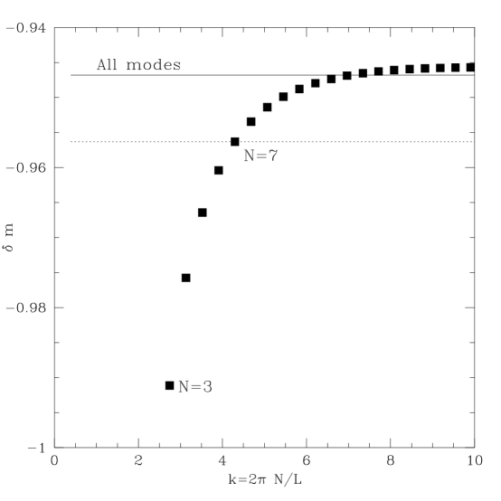
FIG. 3.: Convergence of the computation of $\delta m$ with cutoff $k=2\pi N/L$ in a plane wave basis. Solid line shows the result including all modes in the box: dashed line indicates one per cent error, which is reached by $N=7$.

Figure 3 shows the convergence of the ‘improved’ result as a function of the cutoff $k$. The horizontal line shows the full result obtained by including all modes in the box. The squares show the ‘improved’ result obtained for limited numbers of $k$ vectors, and $N$ labels the cutoff mode number, with $k=2\pi N/L$. The ‘improved’ result is within one per cent of the full result when we include modes up to N=7, or $k\sim 5$.

Our technique clearly works very well for the $\phi^{4}$ kink in one spatial dimension, and could be applied with similar ease to any other one dimensional scalar field theory with kinks. The convergence of the ‘improved’ formula for $\delta m$ with the cutoff in $k$ space augurs well for the prospect of performing analogous calculations in three dimensions. Just as here, the high $k$ contributions can be computed analytically. And if the convergence is similar, we can expect to obtain accurate results for the soliton mass corrections using of order $N^{3}\sim 10^{3}$ modes in $k$ space, which should certainly be feasible.

VI Conclusion

We have developed a technique for calculating the first quantum correction to the mass of a static soliton. This technique is implementable for arbitrary stable solitons within a broad class of Lagrangians. As an example, we applied this technique to the $\phi^{4}$ kink, where the result is known analytically: the numerical answer agreed well with the correct one. We hope to use this technique to calculate quantum corrections to the masses of more complicated solitons in three spatial dimensions.

REFERENCES

- [1]
- [2] J.F Donoghue, E. Golowich and B.R. Holstein, Dynamics of the Standard Model, Cambridge University Press (1992).
- [3] T. H. R. Skyrme, Proc. Roy. Soc. 260 (1961) 127
- [4] E. Braaten, S. Townsend and L. Carson, Phys. Lett. B235 (1990) 147; R. Battye and P. Sutcliffe, Imperial preprint 96-97/18, hep-th/9702089, Phys. Rev. Lett. (1997).
- [5] C. Barnes, W.K. Baskerville, N. Turok, Phys. Rev. Lett. 79(3)(1997) 367-370; C. Barnes, K. Baskerville and N. Turok, preprint hep-th/9704028, Phys. Lett. B, in press (1997).
- [6] R. Rajaraman, Solitons and Instantons, Chaps. 5-8, Elsevier, 1987.
- [7] R. Dashen, B. Hasslacher and A. Neveu, Phys. Rev. D10 (1974) 4130. A recent reference is A. Rebhan and P. van Nieuwenhuizen, hep-th/9707163.
- [8] K. Cahill, A. Comtet, R. Glauber Phys. Lett. B 64(1976) 283
- [9] F. Scholtz, B. Schwesinger, B. Geyer, Nuc. Phys. A 561(1993) 542
- [10] M. Holzwarth, Phys. Lett. B 291(1992) 218
- [11] P. M. Morse and H. F. Feshbach, Methods of Theoretical Physics, McGraw-Hill, 1953.
- [12] W. Press, S. Teukolsky, W. Vetterling, B. Flannery Numerical Recipies, 2nd Ed., Chapter 19, Cambridge University Press, 1988.
- [13] C.Barnes and N.Turok, in progress.