Chapter 1 INLO-PUB-10/97
GRIBOV AMBIGUITIES AND THE FUNDAMENTAL DOMAIN

DEDICATED TO THE MEMORY OF VLADIMIR GRIBOV

1 INTRODUCTION

Non-perturbative aspects are believed to play a crucial role in understanding the formation of a mass gap in the spectrum of excitations in a non-Abelian gauge theory, but despite much progress a simple explanation is still lacking. Here this problem will be addressed in a finite volume, where its size can be used as a control parameter, which is absent in infinite volumes. The starting point, as in solving a quantum mechanical problem, is finding a proper description of the classical potential and its minima.

Due to the non-Abelian nature of the theory not only the classical potential, but also the kinetic term in the Lagrangian or Hamiltonian, is more complicated. The latter is a manifestation of the non-trivial Riemannian geometry of the physical configuration space[1], formed by the set of gauge orbits $\cal{A}/\cal{G}$ ($\cal{A}$ is the collection of connections, $\cal{G}$ the group of local gauge transformations). Most frequently, coordinates of this orbit space are chosen by picking a representative gauge field on the orbit in a smooth and preferably unique way. It is by now well known that linear gauge conditions like the Landau or Coulomb gauge suffer from Gribov ambiguities[2]. The reason behind this is that topological obstructions prevent one from introducing affine coordinates[3] in a global way. In principle therefore, one can introduce different coordinate patches with transition functions to circumvent this problem[4]. One way to make this specific is to base the coordinate patches on the choice of a background gauge condition[5, 6]. One could envisage to associate to each coordinate patch ghost fields and extend BRST symmetry to include fields with non-trivial “Grassmannian sections”, although such a formulation is still in its infancy.

We will pursue, however, the issue of finding a fundamental domain for non-Abelian gauge theories[7] and its consequence for the glueball spectrum in intermediate volumes. The finite volume context allows us to make reliable statements on the non-perturbative contributions, because asymptotic freedom guarantees that at small volumes the effective coupling constant is small, such that high-momentum states can be treated perturbatively. Only the lowest (typically zero or near-zero momentum) states will be affected by non-perturbative corrections. We emphasize that it is essential that gauge invariance is implemented properly at all stages. We will describe the results mainly in the context of a Hamiltonian picture[8] with wave functionals on configuration space. Although rather cumbersome from a perturbative point of view, where the covariant path integral approach of Feynman is vastly superior, it provides more intuition on how to deal with non-perturbative contributions to observables that do not vanish in perturbation theory. An essential feature of the non-perturbative behaviour is that the wave functional spreads out in configuration space to become sensitive to its non-trivial geometry. If wave functionals are localised within regions much smaller than the inverse curvature of the field space, the curvature has no effect on the wave functionals. At the other extreme, if the configuration space has non-contractible circles, the wave functionals are drastically affected by the geometry, or topology, when their support extends over the entire circle. Instantons are of course the most important examples of this. Not only the vacuum energy is affected by these instantons, but also the low-lying glueball states and this is what we are after to describe accurately, albeit in sufficiently small volumes. The geometry of the finite volume, to be considered here, is the one of a three-torus[9, 5] and a three-sphere[10, 11]. These lecture notes are an updated and extended version of ref [12].

2 COMPLETE GAUGE FIXING

An (almost) unique representative of the gauge orbit is found by minimising the $L^{2}$ norm of the vector potential along the gauge orbit[7, 13]

$$F_{A}(g)~{}\equiv\left\|{}^{g}A\right\|^{2}~{}=~{}-\int_{M}d^{3}x~{}\mbox{\,tr\,}\left(\left(g^{-1}A_{i}g+g^{-1}\partial_{i}g\right)^{2}\right),$$ (1)

where the vector potential is taken anti-hermitian. Expanding around the minimum of eq. (1), writing $g(x)=\exp(X(x))$, one easily finds:

$$\left\|{}^{g}A\right\|^{2} = \left\|A\right\|^{2}+2\int_{M}\mbox{\,tr\,}(X\partial_{i}A_{i})+\int_{M}\mbox{\,tr\,}(X^{\dagger}FP(A)X)$$ (2)

$$+\frac{1}{3}\int_{M}\mbox{\,tr\,}\left(X\left[[A_{i},X],\partial_{i}X\right]\right)+\frac{1}{12}\int_{M}\mbox{\,tr\,}\left([D_{i}X,X][\partial_{i}X,X]\right)+\mbox{$\cal O$}\left(X^{5}\right).$$

Where $FP(A)$ is the Faddeev-Popov operator $({\rm ad}(A)X~{}\equiv~{}[A,X])$

$$FP(A)~{}=~{}-\partial_{i}D_{i}(A)~{}=~{}-\partial^{2}_{i}-\partial_{i}{\rm ad}(A_{i}).$$ (3)

At any local minimum the vector potential is therefore transverse, $\partial_{i}A_{i}~{}=~{}0$, and $FP(A)$ is a positive operator. The set of all these vector potentials is by definition the Gribov region $\Omega$. Using the fact that $FP(A)$ is linear in $A$, $\Omega$ is seen to be a convex subspace of the set of transverse connections $\Gamma$. Its boundary $\partial\Omega$ is called the Gribov horizon. At the Gribov horizon, the lowest eigenvalue of the Faddeev-Popov operator vanishes, and points on $\partial\Omega$ are hence associated with coordinate singularities. Any point on $\partial\Omega$ can be seen to have a finite distance to the origin of field space and in some cases even uniform bounds can be derived[14, 15].

The Gribov region is the set of local minima of the norm functional (3) and needs to be further restricted to the absolute minima to form a fundamental domain, which will be denoted by $\Lambda$. The fundamental domain is clearly contained within the Gribov region. To show that also $\Lambda$ is convex we note that

$$\left\|{}^{g}A\right\|^{2}-\left\|A\right\|^{2} = \int\mbox{\,tr\,}\left(A_{i}^{2}\right)-\int\mbox{\,tr\,}\left(\left(g^{-1}A_{i}g+g^{-1}\partial_{i}g\right)^{2}\right)$$ (4)

$$= \int\mbox{\,tr\,}\left(g^{\dagger}FP_{f}(A)~{}g\right)\equiv\left\langle g,FP_{f}(A)~{}g\right\rangle,$$

where $FP_{f}(A)$ is the Faddeev-Popov operator generalised to the fundamental representation. At the critical points $A\in\Gamma$ of the norm functional (recall $\Gamma=\{A\in\mbox{$\cal A$}|\partial_{i}A_{i}=0\}$) $FP_{f}(A)$, like $FP(A)$, is a hermitian operator. We can define $\Lambda$ in terms of the absolute minima over $g\in\mbox{$\cal G$}$ of $\left\langle g,FP_{f}(A)~{}g\right\rangle$

$$\Lambda=\{A\in\Gamma|\min_{g\in\mbox{$\cal G$}}\left\langle g,FP_{f}(A)~{}g\right\rangle=0\}.$$ (5)

Using that $FP_{f}(A)$ is linear in $A$ and assuming that $A^{(1)}$ and $A^{(2)}$ are in $\Lambda$ and therefore satisfy the equation $\min_{g\in\mbox{$\cal G$}}\left\langle g,FP_{f}(A)~{}g\right\rangle=0$, we find that $A=sA^{(1)}+(1-s)A^{(2)}$ satisfies the same identity for all $s\in[0,1]$ (such that both $s$ and $(1-s)$ are positive). The line connecting two points in $\Lambda$, therefore lies within $\Lambda$.

If we would not specify anything further, as a convex space is contractible, the fundamental region could never reproduce the non-trivial topology of the configuration space. This means that $\Lambda$ should have a boundary[16]. Indeed, as $\Lambda$ is contained in $\Omega$, this means $\Lambda$ is also bounded in each direction. Clearly $A=0$ is in the interior of $\Lambda$, which allows us to consider a ray extending out from the origin into a given direction, where it will have to cross the boundary of $\Lambda$ and $\Omega$. For any point along this ray in $\Lambda$, the norm functional is at its absolute minimum as a function of the gauge orbit. However, for points in $\Omega$ that are not also in $\Lambda$, the norm functional is necessarily at a relative minimum. The absolute minimum for this orbit is an element of $\Lambda$, but in general not along the ray. Continuity therefore tells us that at some point along the ray, this absolute minimum has to pass the local minimum. At the point they are exactly degenerate, there are two gauge equivalent vector potentials with the same norm, both at the absolute minimum. As in the interior the norm functional has a unique minimum, again by continuity, these two degenerate configurations have to both lie on the boundary of $\Lambda$. This is the generic situation.

It is important to note that $A=0$ is a so-called reducible connection[17] which has a non-trivial stabiliser, i.e. a subgroup of the gauge group that leaves the connection invariant, in this case the set of constant gauge transformations. These reducible connections give rise to so-called orbifold singularities, that manifest themselves through curvature singularities. We know perfectly well how to deal with it by not fixing the constant gauge transformations. Indeed the norm functional is degenerate along the constant gauge transformations and the Coulomb gauge does not fix this gauge degree of freedom. We simply demand that the wave functional is in the singlet representation under the constant gauge transformations. The degeneracy of the norm functional along the constant gauge transformations gives rise to a trivial part in the kernel of the Faddeev-Popov operator (also directly seen by inspection, since it vanishes when acting on constant Lie-algebra elements that generate the constant gauge transformations). This trivial kernel is to be projected out, something that is possible in a finite volume. In this formalism there is a remnant gauge invariance $G$, which requires no gauge fixing since its volume is finite, but still needs to be divided out to get the proper identification

$$\Lambda/G~{}=~{}\cal{A}/\cal{G}.$$ (6)

Here $\Lambda$ is assumed to include the non-trivial boundary identifications. It is these boundary identifications that restore the non-trivial topology of $\cal{A}/\cal{G}$.

If the degeneracy at the boundary is continuous along non-trivial directions one necessarily has at least one non-trivial zero eigenvalue for $FP(A)$ and the Gribov horizon will touch the boundary of the fundamental domain at these so-called singular boundary points. We sketch the general situation in figure 1. By singular we mean here a coordinate singularity. In principle, by choosing a different gauge fixing in the neighbourhood of these points one could resolve the singularity. If singular boundary points would not exist, all that would have been required is to complement the Hamiltonian in the Coulomb gauge with the appropriate boundary conditions in field space. Since the boundary identifications are by gauge transformations the boundary condition on the wave functionals is simply that they are identical under the boundary identifications, possibly up to a phase in case the gauge transformation is homotopically non-trivial, as will be discussed further on in more detail.

Figure 1: Sketch of the Gribov and fundamental regions. The dotted lines indicate the boundary identifications.

Unfortunately, the existence of non-contractible spheres[3] in the configuration space allows one to argue that singular boundary points are to be expected[16]. Consider the intersection of a $d$-dimensional non-contractible sphere with $\Lambda$. The part in the interior of $\Lambda$ is contractible and it can only become non-contractible through the boundary identifications. The simplest way this can occur[16] is if for the ($d$-1)-dimensional intersection with the boundary, all points are to be identified. It would imply degeneracy of the the norm functional on a ($d$-1)-dimensional subspace, leading to at least $d$-1 zero-modes for the Faddeev-Popov operator. The intersection with the boundary of $\Lambda$ can, however, exist of more than one connected component. In the case of two such components one can make a non-contractible sphere by identifying points of the ($d$-1)-dimensional boundary intersection of the first connected component with that of the second and there is no necessity for a continuous degeneracy. Conversely, not all singular boundary points, even those associated with continuous degeneracies, need to be associated with non-contractible spheres.

When a singular boundary point is not associated to a continuous degeneracy, the norm functional undergoes a bifurcation moving from inside to outside the fundamental (and Gribov) region. The absolute minimum turns into a saddle point and two local minima appear, as indicated in figure 2. These are necessarily gauge copies of each other. The gauge transformation is homotopically trivial as it reduces to the identity at the bifurcation point, evolving continuously from there on. For reducible connections, that have a non-trivial stabiliser, this argument may be false[18], but examples of bifurcations at irreducible connections were explicitly found for $S^{3}$, see ref.[19] (app. A). We will come back to this.

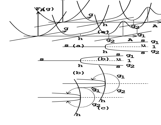
Figure 2: Sketch of a singular boundary point due to a bifurcation of the norm functional. It can be used to show that there are homotopically trivial gauge copies inside the Gribov horizon ($h$).

Also Gribov’s original arguments for the existence of gauge copies[2] (showing that points just outside the horizon are gauge copies of points just inside) can be easily understood from the perspective of bifurcations in the norm functional. It describes the generic case where the zero-mode of the Faddeev-Popov operator arises because of the coalescence of a local minimum with a saddle point with only one unstable direction. At the Gribov horizon the norm functional locally behaves in that case as $X^{3}$, with $X$ the relevant zero eigenfunction of the Faddeev-Popov operator. The situation sketched in figure 2 corresponds to the case where the leading behaviour is like $X^{4}$. See ref.[16] for more details and a discussion of the Morse theory aspects that simplify the bifurcation analysis. As the Gribov region is associated with the local minima, and since the space of gauge transformations resembles that of a spin model, the analogy with spin glasses makes it unreasonable to expect that the Gribov region is free of further gauge copies. This will be illustrated by explicit examples. Unfortunately restrictions to a subset of the transverse gauge fields is a rather non-local procedure. This cannot be avoided since it reflects the non-trivial topology of field space.

3 GAUGE FIELDS ON THE THREE-TORUS

Homotopical non-trivial gauge transformations are in one to one correspondence with non-contractible loops in configuration space, which give rise to conserved quantum numbers. The quantum numbers are like the Bloch momenta in a periodic potential and label representations of the homotopy group of gauge transformations. On the fundamental domain the non-contractible loops arise through identifications of boundary points (as will be demonstrated quite explicitly for the torus in the zero-momentum sector). Although slightly more hidden, the fundamental domain will therefore contain all the information relevant for the topological quantum numbers. Sufficiently accurate knowledge of the boundary identifications will allow for an efficient and natural projection on the various superselection sectors (i.e. by choosing the appropriate “Bloch wave functionals”). All these features were at the heart of the finite volume analysis on the torus[5] and we see that they can in principle be naturally extended to the full theory, thereby including the desired $\theta$ dependence. In the next section this will be discussed in the context of the three-sphere. In ref.[6] we proposed formulating the Hamiltonian theory on coordinate patches, with homotopically non-trivial gauge transformations as transition functions. Working with boundary conditions on the boundary of the fundamental domain is easily seen to be equivalent and conceptually much simpler to formulate. If there would be no singular boundary points this would have provided a Hamiltonian formulation where all topologically non-trivial information can be encoded in the boundary conditions. Still, for the low-lying states in a finite volume, both on the three-torus and the three-sphere, singular boundary points will not play an important role in intermediate volumes.

Probably the most simple example to illustrate the relevance of the fundamental domain is provided by gauge fields on the torus in the abelian zero-momentum sector. For definiteness let us take $G=SU(2)$ and $A_{i}=i{C_{i}\over 2L}\tau_{3}$ ($L$ is the size of the torus). These modes are dynamically motivated as they form the set of gauge fields on which the classical potential vanishes. It is called the vacuum valley (sometimes also referred to as toron valley) and one can attempt to perform a Born-Oppenheimer-like approximation for deriving an effective Hamiltonian in terms of these “slow” degrees of freedom. To find the Gribov horizon, one easily verifies that the part of the spectrum for $FP(A)$ that depends on $\vec{C}$, is given by $\lambda^{gh}_{\vec{n}}(\vec{C})=2\pi\vec{n}\cdot(2\pi\vec{n}\pm\vec{C})$, with $\vec{n}\neq\vec{0}$ an integer vector. The lowest eigenvalue therefore vanishes if $C_{k}=\pm 2\pi$. The Gribov region is therefore a cube with sides of length $4\pi$, centred at the origin, specified by $|C_{k}|\leq 2\pi$ for all $k$, see figure 3.

The gauge transformation $g_{(k)}=\exp(\pi ix_{k}\tau_{3}/L)$ maps $C_{k}$ to $C_{k}+2\pi$, leaving the other components of $\vec{C}$ untouched. As $g_{(k)}$ is anti-periodic it is homotopically non-trivial (they are ’t Hooft’s twisted gauge transformations[20]). We thus see explicitly that gauge copies occur inside $\Omega$, but furthermore the naive vacuum $A=0$ has (many) gauge copies under these shifts of $2\pi$ that lie on the Gribov horizon. It can actually be shown for the Coulomb gauge that for any three-manifold, any Gribov copy by a homotopically non-trivial gauge transformation of $A=0$ will have vanishing Faddeev-Popov determinant[16]. Taking the symmetry under homotopically non-trivial gauge transformations properly into account is crucial for describing the non-perturbative dynamics and one sees that the singularity of the Hamiltonian at Gribov copies of $A=0$, where the wave functionals are in a sense maximal, could form a severe obstacle in obtaining reliable results.

To find the boundary of the fundamental domain we note that the gauge copies $\vec{C}=(\pi,C_{2},C_{3})$ and $\vec{C}=(-\pi,C_{2},C_{3})$ have equal norm. The boundary of the fundamental domain, restricted to the vacuum valley formed by the abelian zero-momentum gauge fields, therefore occurs where $|C_{k}|=\pi$, well inside the Gribov region, see figure 3. The boundary identifications are by the homotopically non-trivial gauge transformations $g_{(k)}$. The fundamental domain, described by $|C_{k}|\leq\pi$, with all boundary points regular, has the topology of a torus. To be more precise, as the remnant of the constant gauge transformations (the Weyl group) changes $\vec{C}$ to $-\vec{C}$, the fundamental domain $\Lambda/G$ restricted to the abelian constant modes is the orbifold $T^{3}/Z_{2}$. Generalisations to arbitrary gauge groups were considered in ref.[6]. (The fundamental domain turns out to coincide with the unit cell or “minimal” coordinate patch defined in ref.[6]).

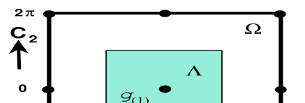
Figure 3: A two dimensional slice of the vacuum valley along the $(C_{1},C_{2})$ plane. The fat square give the Gribov horizon, the grey square is the fundamental domain. The dots at the Gribov horizon are Gribov copies of the origin.

Formulating the Hamiltonian on $\Lambda$, with the boundary identifications implied by the gauge transformations $g_{(k)}$, avoids the singularities at the Gribov copies of $A=0$. “Bloch momenta” associated to the $2\pi$ shift, implemented by the non-trivial homotopy of $g_{(k)}$, label ‘t Hooft’s electric flux quantum numbers[20] $\Psi(C_{k}=-\pi)=\exp(\pi ie_{k})\Psi(C_{k}=\pi)$. Note that the phase factor is not arbitrary, but $\pm 1$. This is because $g^{2}_{(k)}$ is homotopically trivial. In other words, the homotopy group of these anti-periodic gauge transformations is $Z_{2}^{3}$. Considering a slice of $\Lambda$ can obscure some of the topological features. A loop that winds around the slice twice is contractible in $\Lambda$ as soon as it is allowed to leave the slice. Indeed including the lowest modes transverse to this slice will make the $Z_{2}$ nature of the relevant homotopy group evident[5]. It should be mentioned that for the torus in the presence of fields in the fundamental representation (quarks), only periodic gauge transformations are allowed. In that case it is easily seen that the intersection of the fundamental domain with the constant abelian gauge fields is given by the domain $|C_{k}|\leq 2\pi$, whose boundary coincides with the Gribov horizon. It is interesting to note that points on $\partial\Omega$ form an explicit example of a continuous degeneracy due to a non-contractible sphere[15].

In weak coupling Lüscher[9] showed unambiguously that the wave functionals are localised around $A=0$, that they are normalisable and that the spectrum is discrete. In this limit the spectrum is insensitive to the boundary identifications (giving rise to a degeneracy in the topological quantum numbers). This is manifested by a vanishing electric flux energy, defined by the difference in energy of a state with $|\vec{e}|=1$ and the vacuum state with $\vec{e}=\vec{0}$. Although there is no classical potential barrier to achieve this suppression, it comes about by a quantum induced barrier, in strength down by two powers of the coupling constant. This gives a suppression[21] with a factor $\exp(-S/g)$ instead of the usual factor of $\exp(-8\pi^{2}/g^{2})$ for instantons[22]. Here $S=12.4637$ is the action computed from the effective potential. At stronger coupling the wave functional spreads out over the vacuum valley and the boundary conditions drastically change the spectrum[5]. At this point the energy of electric flux suddenly switches on.

Integrating out the non-zero momentum degrees of freedom, for which Bloch degenerate perturbation theory provides a rigorous framework[23, 9], one finds an effective Hamiltonian. Near $A=0$, due to the quartic nature of the potential energy $(F^{a}_{ij})^{2}$ for the zero-momentum modes (the derivatives vanish and the field strength is quadratic in the field), there is no separation in time scales between the abelian and non-abelian modes. Away from $A=0$ one could further reduce the dynamics to one along the vacuum valley, but near the origin this would be a singular decomposition (the adiabatic approximation breaks down). However, as long as the coupling constant is not too large, the wave functional can be reduced to a wave function on the vacuum valley near $\partial\Lambda$ where the boundary conditions can be implemented. These boundary conditions are formulated in a manner that preserves the invariance under constant gauge transformation and the effective Hamiltonian is solved by Rayleigh-Ritz (providing also lower bounds from the second moment of the Hamiltonian). The influence of the boundary conditions on the low-lying glueball states is felt as soon as the volume is bigger than an inverse scalar glueball mass. We summarise below the ingredients that enter the calculations.

The effective Hamiltonian is expressed in terms of the coordinates $c_{i}^{a}$, where $i=\{1,2,3\}$ is the spatial index ($c_{0}=0$) and $a=\{1,2,3\}$ is the SU(2)-colour index. These coordinates are related to the zero-momentum gauge fields through $A_{i}^{a}(x)=c_{i}^{a}/L$. We note that the field strength is given by $F_{ij}^{a}=-\varepsilon_{abd}c_{i}^{b}c_{j}^{d}/L^{2}$ and we introduce the gauge-invariant “radial” coordinate $r_{i}=\sqrt{\sum_{a}c_{i}^{a}c_{i}^{a}}$. The latter will play a crucial role in specifying the boundary conditions. For dimensional reasons the effective Hamiltonian is proportional to $1/L$. It will furthermore depend on $L$ through the renormalised coupling constant ($g(L)$) at the scale $\mu=1/L$. To one-loop order one has (for small $L$) $g(L)^{2}=12\pi^{2}/[-11\ln(\Lambda_{MS}L)]$. One expresses the masses and the size of the finite volume in dimensionless quantities, like mass-ratios and the parameter $z=mL$. In this way, the explicit dependence of $g$ on $L$ is irrelevant. This is also the preferred way of comparing results obtained within different regularisation schemes (i.e. dimensional and lattice regularisation). The effective Hamiltonian is now given by

$$L\cdot H_{eff}(c) = {g^{2}\over 2(1+\alpha_{1}g^{2})}\sum_{i,a}{\partial^{2}\over\partial{c_{i}^{a}}^{2}}+{1\over 4}({1\over g^{2}}+\alpha_{2})\sum_{ij,a}{F_{ij}^{a}}^{2}$$ (7)

$$+\gamma_{1}\sum_{i}r_{i}^{2}+\gamma_{2}\sum_{i}r_{i}^{4}+\gamma_{3}\sum_{i>j}r_{i}^{2}r_{j}^{2}+\gamma_{4}\sum_{i}r_{i}^{6}+\gamma_{5}\sum_{i\neq j}r_{i}^{2}r_{j}^{4}+\gamma_{6}\prod_{i}r_{i}^{2}$$

$$+\alpha_{3}\sum_{ijk,a}r_{i}^{2}{F_{jk}^{a}}^{2}+\alpha_{4}\sum_{ij,a}r_{i}^{2}{F_{ij}^{a}}^{2}+\alpha_{5}{\det}^{2}c.$$

We have organised the terms according to the importance of their contributions, ignoring terms quartic in the momenta. The first line gives (when ignoring $\alpha_{1,2}$) the lowest order effective Hamiltonian, whose energy eigenvalues are ${\cal O}(g^{2/3})$, as can be seen by rescaling $c$ with $g^{2/3}$. Thus, in a perturbative expansion $c={\cal O}(g^{2/3})$. The second line includes the vacuum-valley effective potential (i.e. the part that does not vanish on the set of abelian configurations). These two lines are sufficient to obtain the mass-ratios to an accuracy of better than 5%. The third line gives terms of ${\cal O}(g^{4})$ in the effective potential, that vanish along the vacuum-valley. The coefficients (to two-loop order for $\gamma_{i}$) are

$$\gamma_{1}=-3.0104661\cdot 10^{-1}-(g/2\pi)^{2}3.0104661\cdot 10^{-1} \alpha_{1}=+2.1810429\cdot 10^{-2},$$ ,

$$\gamma_{2}=-1.4488847\cdot 10^{-3}-(g/2\pi)^{2}9.9096768\cdot 10^{-3} \alpha_{2}=+7.5714590\cdot 10^{-3},$$ ,

$$\gamma_{3}=+1.2790086\cdot 10^{-2}+(g/2\pi)^{2}3.6765224\cdot 10^{-2} \alpha_{3}=+1.1130266\cdot 10^{-4},$$ ,

$$\gamma_{4}=+4.9676959\cdot 10^{-5}+(g/2\pi)^{2}5.2925358\cdot 10^{-5} \alpha_{4}=-2.1475176\cdot 10^{-4},$$ ,

$$\gamma_{5}=-5.5172502\cdot 10^{-5}+(g/2\pi)^{2}1.8496841\cdot 10^{-4} \alpha_{5}=-1.2775652\cdot 10^{-3},$$ ,

$$\gamma_{6}=-1.2423581\cdot 10^{-3}-(g/2\pi)^{2}5.7110724\cdot 10^{-3}$$ . (8)

The choice of boundary conditions, associated to each of the irreducible representations of the cubic group $O(3,{\rm Z\!\!Z})$ and to the states that carry electric flux[20], is best described by observing that the cubic group is the semidirect product of the group of coordinate permutations $S_{3}$ and the group of coordinate reflections $Z_{2}^{3}$. We denote the parity under the coordinate reflection $c_{i}^{a}\rightarrow-c_{i}^{a}$ by $p_{i}=\pm 1$ ($i$ fixed). The electric flux quantum number for the same direction will be denoted by $q_{i}=\pm 1$. This is related to the more usual additive (mod 2) quantum number $e_{i}$ by $q_{j}=\exp(i\pi e_{j})$. Note that for SU(2) electric flux is invariant under coordinate reflections. If not all of the electric fluxes are identical, the cubic group is broken to $S_{2}\times Z_{2}^{3}$, where $S_{2}(\sim Z_{2})$ corresponds to interchanging the two directions with identical electric flux (unequal to the other electric flux). If all the electric fluxes are equal, the wave functions are irreducible representations of the cubic group. These are the four singlets $A_{1(2)}^{\pm}$, which are completely (anti-)symmetric with respect to $S_{3}$ and have each of the parities $p_{i}=\pm 1$. Then there are two doublets $E^{\pm}$, also with each of the parities $p_{i}=\pm 1$ and finally one has four triplets $T_{1(2)}^{\pm}$. Each of these triplet states can be decomposed into eigenstates of the coordinate reflections. Explicitly, for $T_{1(2)}^{\pm}$ we have one state that is (anti-)symmetric under interchanging the two- and three-directions, with $p_{2}=p_{3}=-p_{1}=\mp 1$. The other two states are obtained through cyclic permutation of the coordinates. Thus, any eigenfunction of the effective Hamiltonian with specific electric flux quantum numbers $q_{i}$ can be chosen to be an eigenstate of the parity operators $p_{i}$. The boundary conditions of these eigenfunctions $\Psi_{\vec{q},\vec{p}}(c)$ are simply given by

$$\Psi_{\vec{q},\vec{p}}(c)|_{{}_{r_{i}=\pi}}=0\quad, \quad{\it if}\quad p_{i}q_{i}=-1$$

$${\partial\over\partial r_{i}}(r_{i}\Psi_{\vec{q},\vec{p}}(c))|_{{}_{r_{i}=\pi}}=0\quad, \quad{\it if}\quad p_{i}q_{i}=+1$$ (9)

and one easily shows that with these boundary conditions the Hamiltonian is hermitian with respect to the innerproduct $<\Psi,\Psi^{\prime}>=\int_{r_{i}\leq\pi}d^{9}c\Psi^{*}(c)\Psi^{\prime}(c)$. For negative parity states ($\prod_{i}p_{i}=-1$) this description is, however, not accurate[24] as parity restricted to the vacuum valley is equivalent to a Weyl reflection (a remnant of the invariance under constant gauge transformations).

Figure 4: Mass ratios $m^{\prime}/m$ as a function of $L$ in units of the inverse scalar glueball mass $m^{-1}$, $z=mL$. The analytic results are given by the full (continuum) and dashed ($4^{3}$ lattice) curves. Represented are the the square root of the energy of electric flux per unit length (bottom), the $E$ tensor mass (middle) and the $T_{2}$ tensor mass (top). The latter two are (almost) degenerate below $z=0.95$, which is also where the electric flux energy is exponentially suppressed. Where no error bars on the Monte Carlo data are visible they are smaller than the size of the data points.

After correcting for lattice artefacts[25], the (semi-)analytic results agree extremely well with the best lattice data[26] (with statistical errors of 2% to 3%) up to a volume of about .75 fermi, or about five times the inverse scalar glueball mass. In figure 4 we present the comparison for a lattice of spatial size $4^{3}$. Monte Carlo data[26] are most accurate for this lattice size. For more detailed comparisons see ref.[25]. The analytic results below $z=0.95$ are due to Lüscher and Münster[27], which is where the spectrum is insensitive to the identifications at the boundary of $\Lambda$.

Most conspicuously the tensor state in finite volumes is split in a doublet $E$, with a mass that is roughly 0.9 times the scalar $A_{1}$ mass and a triplet $T_{2}$ with a mass of roughly 1.7 times the scalar mass. Note that the multiplicity weighted average is approximately 1.4 times the scalar mass, agreeing well with what was found at large volumes from lattice data[26].

Apart from the corrections for the lattice artefacts, generalisation to SU(3) was established by Vohwinkel[28], with qualitatively similar results. In large volumes the rotational symmetry should be restored, as is observed from lattice simulations. The properties of the fundamental domain restricted to the zero-momentum modes for $SU(3)$ can be read off from the results in ref.[6]. In this reference also the generalisation to arbitrary gauge groups is discussed.

At large volumes extra degrees of freedom start to behave non-perturbatively. To demonstrate this, the minimal barrier height that separates two vacuum valleys that are related by gauge transformations with non-trivial winding number

$$\nu(g)={1\over 24\pi^{2}}\int_{M}\mbox{\,Tr\,}((g^{-1}dg)^{3}),$$ (10)

was found to be $72.605/Lg^{2}$, using the lattice approximation and carefully taking the continuum limit[29]. As long as the states under consideration have energies below this value, the transitions over this barrier can be neglected and the zero-momentum effective Hamiltonian provides an accurate description. One can now easily find for which volume the energy of the level that determines the glueball mass (defined by the difference with the groundstate energy) starts to be of the order of this barrier height. This turns out to be the case for $L$ roughly 5 to 6 times the correlation length set by the scalar glueball mass. The situation is sketched in figure 5.

We expect, as will be shown for the three-sphere, that the boundary of the fundamental domain along the path in field space across the barrier (which corresponds to the instanton path if we parametrise this path by Euclidean time $t$), occurs at the saddle point (which we call a finite volume sphaleron) in between the two minima. The degrees of freedom along this tunnelling path go outside of the space of zero-momentum gauge fields and if the energy of a state flows over the barrier, its wave functional will no longer be exponentially suppressed below the barrier and will in particular be non-negligible at the boundary of the fundamental domain. Boundary identifications in this direction of field space now become dynamically important too. The relevant “Bloch momentum” is in this case obviously the $\theta$ parameter, as wave functionals pick up a phase factor $e^{i\theta}$ under a gauge transformation with winding number one. For many of the intricacies in describing instantons on a torus we refer to ref.[30, 31, 32]. On the three-torus we have therefore achieved a self-contained picture of the low-lying glueball spectrum in intermediate volumes from first principles with no free parameters, apart from the overall scale.

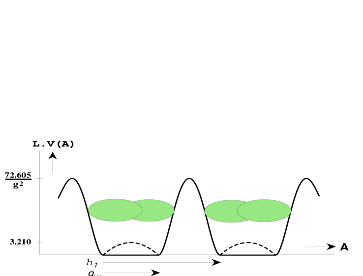
Figure 5: “Artistic impression” of the potential for the three-torus. Shown are two vacuum valleys, related to each other by a gauge transformation $h_{1}$ with winding number 1, whose shape in the direc- tion perpendicular to the valley depends on the position along the valley. The induced one-loop effec- tive potential, of height $3.210/L$, has degenerate minima related to each other by the anti-periodicgauge transformations $g_{(k)}$. The classical barrier, separating the two valleys, has a height $72.605/Lg^{2}$.

4 GAUGE FIELDS ON THE THREE-SPHERE

The reason to consider the three-sphere lies in the fact that the conformal equivalence of $S^{3}\times{\rm I\kern-1.79993ptR}$ to ${\rm I\kern-1.79993ptR}^{4}$ allows one to construct instantons explicitly[11, 33]. This greatly simplifies the study of how to formulate $\theta$ dependence in terms of boundary conditions on the fundamental domain, and indeed we will see that for $S^{3}$ simple enough results can be obtained to address this question[19, 34]. The disadvantage of the three-sphere is that in large volumes the corrections to the glueball masses are no longer exponential[9].

We will summarise the formalism that was developed in[11]. Alternative formulations, useful for diagonalising the Faddeev-Popov and fluctuation operators, were given in ref.[10]. We embed $S^{3}$ in ${\rm I\kern-1.79993ptR}^{4}$ by considering the unit sphere parametrised by a unit vector $n_{\mu}$. It is particularly useful to introduce the unit quaternions $\sigma_{\mu}$ and their conjugates $\bar{\sigma}_{\mu}=\sigma^{\dagger}_{\mu}$ by

$$\sigma_{\mu}=(\mbox{$id$},i\vec{\tau}),\hskip 42.67912pt\bar{\sigma}_{\mu}=(\mbox{$id$},-i\vec{\tau}).$$ (11)

They satisfy the multiplication rules

$$\sigma_{\mu}\bar{\sigma}_{\nu}=\eta^{\alpha}_{\mu\nu}\sigma_{\alpha},\hskip 42.67912pt\bar{\sigma}_{\mu}\sigma_{\nu}=\bar{\eta}^{\alpha}_{\mu\nu}\sigma_{\alpha},$$ (12)

where we used the ’t Hooft $\eta$ symbols[22], generalised slightly to include a component symmetric in $\mu$ and $\nu$ for $\alpha=0$. We can use $\eta$ and $\bar{\eta}$ to define orthonormal framings[35] of $S^{3}$, which were motivated by the particularly simple form of the instanton vector potentials in these framings. The framing for $S^{3}$ is obtained from the framing of ${\rm I\kern-1.79993ptR}^{4}$ by restricting in the following equation the four-index $\alpha$ to a three-index $a$ (for $\alpha=0$ one obtains the normal on $S^{3}$):

$$e^{\alpha}_{\mu}=\eta^{\alpha}_{\mu\nu}n_{\nu},\hskip 42.67912pt\bar{e}^{\alpha}_{\mu}=\bar{\eta}^{\alpha}_{\mu\nu}n_{\nu}.$$ (13)

Note that $e$ and $\bar{e}$ have opposite orientations. Each framing defines a differential operator and associated (mutually commuting) angular momentum operators $\vec{L}_{1}$ and $\vec{L}_{2}$:

$$\partial^{i}=e^{i}_{\mu}\frac{\partial}{\partial x^{\mu}},\quad L_{1}^{i}=\frac{i}{2}~{}\partial^{i}\quad,\quad\bar{\partial}^{i}=\bar{e}^{i}_{\mu}\frac{\partial}{\partial x^{\mu}},\quad L_{2}^{i}=\frac{i}{2}~{}\bar{\partial}^{i}.$$ (14)

It is easily seen that $\vec{L}_{1}^{2}=\vec{L}_{2}^{2}$, which has eigenvalues $l(l+1)$, with $l=0,{\scriptstyle{{1\over 2}}},1,\cdots$.

The (anti-)instantons[36] in these framings, obtained from those on ${\rm I\kern-1.79993ptR}^{4}$ by interpreting the radius in ${\rm I\kern-1.79993ptR}^{4}$ as the exponential of the time $t$ in the geometry $S^{3}\times{\rm I\kern-1.79993ptR}$, become

$$A_{0}=\frac{\vec{\varepsilon}\cdot\vec{\sigma}}{2(1+\varepsilon\cdot n)},\hskip 42.67912pt\vec{A}=\frac{\vec{\sigma}\wedge\vec{\varepsilon}-(u+\varepsilon\cdot n)\vec{\sigma}}{2(1+\varepsilon\cdot n)},$$ (15)

where

$$u=\frac{2s^{2}}{1+b^{2}+s^{2}},\hskip 42.67912pt\varepsilon_{\mu}=\frac{2sb_{\mu}}{1+b^{2}+s^{2}},\hskip 42.67912pts=\lambda e^{t}.$$ (16)

Here $\vec{\varepsilon}$ and $\vec{A}$ are defined with respect to the framing $e^{a}_{\mu}$ for instantons and with respect to the framing $\bar{e}^{a}_{\mu}$ for anti-instantons. The instanton describes tunnelling from $A=0$ at $t=-\infty$ to $A_{a}=-\sigma_{a}$ at $t=\infty$, over a potential barrier at $t=0$ that is lowest when $b_{\mu}\equiv 0$. This configuration corresponds to a sphaleron[37], i.e. the vector potential $A_{a}=-{\scriptstyle{{1\over 2}}}\sigma_{a}$ is a saddle point of the energy functional with one unstable mode, corresponding to the direction ($u$) of tunnelling. At $t=\infty$, $A_{a}=-\sigma_{a}$ has zero energy and is a gauge copy of $A_{a}=0$ by a gauge transformation $g=n\cdot\bar{\sigma}$ with winding number one.

We will be concentrating our attention to the modes that are degenerate in energy to lowest order with the modes that describe tunnelling through the sphaleron and ”anti-sphaleron”. The latter is a gauge copy by a gauge transformation $g=n\cdot\sigma$ with winding number $-1$ of the sphaleron. The two dimensional space containing the tunnelling paths through these sphalerons is consequently parametrised by $u$ and $v$ through

$$A_{\mu}(u,v)=\left(-ue^{a}_{\mu}-v\bar{e}^{a}_{\mu}\right)\frac{\sigma_{a}}{2}.$$ (17)

The gauge transformation with winding number $-1$ is easily seen to map $(u,v)=(w,0)$ into $(u,v)=(0,2-w)$. The 18 dimensional space is defined by

$$A_{\mu}(c,d)=\left(c^{a}_{i}e^{i}_{\mu}+d^{a}_{j}\bar{e}^{j}_{\mu}\right)\frac{\sigma_{a}}{2}=A_{i}(c,d)e_{\mu}^{i}.$$ (18)

The $c$ and $d$ modes are mutually orthogonal and satisfy the Coulomb gauge condition:

$$\partial_{i}A_{i}(c,d)=0.$$ (19)

This space contains the $(u,v)$ plane through $c^{a}_{i}=-u\delta^{a}_{i}$ and $d^{a}_{i}=-v\delta^{a}_{i}$. The significance of this 18 dimensional space is that the energy functional[11]

$$\mbox{$\cal V$}(c,d)\equiv-\int_{S^{3}}\frac{1}{2}\mbox{\,tr\,}(F_{ij}^{2})=\mbox{$\cal V$}(c)+\mbox{$\cal V$}(d)+\frac{2\pi^{2}}{3}\left\{(c^{a}_{i})^{2}(d^{b}_{j})^{2}-(c^{a}_{i}d^{a}_{j})^{2}\right\},$$ (20)

$$\mbox{$\cal V$}(c)=2\pi^{2}\left\{2(c^{a}_{i})^{2}+6\det c+\frac{1}{4}[(c^{a}_{i}c^{a}_{i})^{2}-(c^{a}_{i}c^{a}_{j})^{2}]\right\},$$ (21)

is degenerate to second order in $c$ and $d$. Indeed, the quadratic fluctuation operator $\cal M$ in the Coulomb gauge, defined by

$$-\int_{S^{3}}\frac{1}{2}\mbox{\,tr\,}(F_{ij}^{2}) = \int_{S^{3}}\mbox{\,tr\,}(A_{i}\mbox{$\cal M$}_{ij}A_{j})+\mbox{$\cal O$}\left(A^{3}\right),$$

$$\mbox{$\cal M$}_{ij} = 2\vec{L}_{1}^{2}\delta_{ij}+2\left(\vec{L}_{1}+\vec{S}\right)^{2}_{ij},\quad S^{a}_{ij}=-i\varepsilon_{aij},$$ (22)

has $A(c,d)$ as its eigenspace for the (lowest) eigenvalue $4$. These modes are consequently the equivalent of the zero-momentum modes on the torus, with the difference that their zero-point frequency does not vanish.

$FP_{f}(A)$ in eq. (4) is defined as a hermitian operator acting on the vector space $\cal L$ of functions $g$ over $S^{3}$ with values in the space of the quaternions ${\rm I\!H}=\{q_{\mu}\sigma_{\mu}|q_{\mu}\in{\rm I\kern-1.79993ptR}\}$. The gauge group $\cal G$ is contained in $\cal L$ by restricting to the unit quaternions: $\mbox{$\cal G$}=\{g\in\mbox{$\cal L$}|g=g_{\mu}\sigma_{\mu},g_{\mu}\in{\rm I\kern-1.79993ptR},g_{\mu}g_{\mu}=1\}$. For arbitrary gauge groups $\cal L$ is defined as the algebra generated by the identity and the (anti-hermitian) generators of the algebra. When minimising the same functional over the larger space $\cal L$ one obviously should find a smaller space $\tilde{\Lambda}\subset\Lambda$. Since $\cal L$ is a linear space $\tilde{\Lambda}$ can also be specified by the condition that $FP_{f}(A)$ be positive,

$$\tilde{\Lambda}=\{A\in\Gamma|\left\langle g,FP_{f}(A)~{}g\right\rangle\geq 0,\ \forall g\in\mbox{$\cal L$}\}.$$ (23)

As for the Gribov horizon, the boundary of $\tilde{\Lambda}$ is therefore determined by the location where the lowest eigenvalue vanishes. For the $(c,d)$ space it can be shown[19] that the boundary $\partial\tilde{\Lambda}$ will touch the Gribov horizon $\partial\Omega$. This establishes the existence of singular points on the boundary of the fundamental domain due to the inclusion $\tilde{\Lambda}\subset\Lambda\subset\Omega$. By showing that the fourth order term in eq. (2) is positive (see app. A of ref.[19]) this is seen to correspond to the situation as sketched in figure 2.

To simplify the notation, write $FP_{f}=FP_{\scriptstyle{{1\over 2}}}$ and $FP=FP_{1}$, with the indices related to the isospin. The associated generators are

$$\vec{T}_{\scriptstyle{{1\over 2}}}={\scriptstyle{{1\over 2}}}\vec{\tau}\qquad\mbox{and}\qquad\vec{T}_{1}={\scriptstyle{{1\over 2}}}{\rm ad}\vec{\tau}.$$ (24)

One can now make convenient use of the ${\rm SU}(2)^{3}$ symmetry generated by $\vec{L}_{1}$, $\vec{L}_{2}$ and $\vec{T}_{t}$ to calculate explicitly the spectrum of $FP_{t}(A)$. One has

$$FP_{t}(A(c,d))=4\vec{L}_{1}^{2}-\frac{2}{t}c^{a}_{i}T_{t}^{a}L_{1}^{i}-\frac{2}{t}d^{a}_{i}T_{t}^{a}L_{2}^{i},$$ (25)

which commutes with $\vec{L}_{1}^{2}=\vec{L}_{2}^{2}$, but for arbitrary $(c,d)$ there are in general no other commuting operators (except for a charge conjugation symmetry when $t={\scriptstyle{{1\over 2}}}$). Restricting to the $(u,v)$ plane one easily finds that

$$FP_{t}(A(u,v))=4\vec{L}_{1}^{2}+\frac{2}{t}u\vec{L}_{1}\cdot\vec{T}_{t}+\frac{2}{t}v\vec{L}_{2}\cdot\vec{T}_{t},$$ (26)

which also commutes with the total angular momentum $\vec{J}_{t}=\vec{L}_{1}+\vec{L}_{2}+\vec{T}_{t}$ and is easily diagonalized. Figure 6 summarises the results for this $(u,v)$ plane and also shows the equal-potential lines as well as exhibiting the multiple vacua and the sphalerons. As it is easily seen that the two sphalerons are gauge copies (by a unit winding number gauge transformation) with equal norm, they lie on $\partial\Lambda$, which can be extend by perturbing around these sphalerons[38].

Figure 6: Location of the classical vacua (large dots), sphalerons (smaller dots), the Gribov horizon (fat sections), the boundary of $\tilde{\Lambda}$ (dashed curves) and part of the boundary of the fundamental domain (full curves). Also indicated are the lines of equal potential in units of $2^{n}$ times the sphaleron energy.

To obtain the result for general $(c,d)$ one can use the invariance under rotations generated by $\vec{L}_{1}$ and $\vec{L}_{2}$ and under constant gauge transformations generated by $\vec{T}_{t}$, to bring $c$ and $d$ to a standard form, or express $\det\left(FP_{t}(A(c,d))|_{l={\scriptstyle{{1\over 2}}}}\right)$, which determines the locations of $\partial\Omega$ and $\partial\tilde{\Lambda}$, in terms of invariants. We define the matrices $X$ and $Y$ by $X^{a}_{b}=(cc^{t})^{a}_{b}$ and $Y^{a}_{b}=(dd^{t})^{a}_{b}$, which allows us to find

$$\det\left(FP_{\scriptstyle{{1\over 2}}}(A(c,d))|_{l={\scriptstyle{{1\over 2}}}}\right) = [81-18\mbox{\,Tr\,}(X+Y)+24(\det c+\det d)$$ (27)

$$-(\mbox{\,Tr\,}(X-Y))^{2}+2\mbox{\,Tr\,}((X-Y)^{2})]^{2}.$$

The two-fold multiplicity is due to charge conjugation symmetry. The expression for $t=1$, that determines the location of the Gribov horizon in the $(c,d)$ space, is given in app. B of ref.[19]. If we restrict to $d=0$ the result simplifies considerably. In that case one can bring $c$ to a diagonal form $c_{i}^{a}=x_{i}\delta_{i}^{a}$. The rotational and gauge symmetry reduce to permutations of the $x_{i}$ and simultaneous changes of the sign of two of the $x_{i}$. One easily finds the invariant expression ($\mbox{\,Tr\,}(X)=\sum_{i}x_{i}^{2}$ and $\det c=\prod_{i}x_{i}$)

$$\det\left(FP_{1}(A(c,0))|_{l={\scriptstyle{{1\over 2}}}}\right)=\left(2\det c-3\mbox{\,Tr\,}(X)+27\right)^{4}.$$ (28)

In figure 7 we present the results for $\Lambda$ and $\Omega$. In this particular case, where $d=0$, $\Lambda$ coincides with $\tilde{\Lambda}$, a consequence of the convexity and the fact that both the sphalerons (indicated by the dots) and the edges of the tetrahedron lie on $\partial\Lambda$, the latter also lying on $\partial\Omega$. It is essential that the sphalerons do not lie on the Gribov horizon and that the potential energy near $\partial\Omega$ is relatively high. This is why we can take the boundary identifications near the sphalerons into account without having to worry about singular boundary points, as long as the energies of the low-lying states will be not much higher than the energy of the sphaleron. It allows one to study the glueball spectrum as a function of the CP violating angle $\theta$, but more importantly it incorporates for $\theta=0$ the noticeable influence of the barrier crossings, i.e. of the instantons.

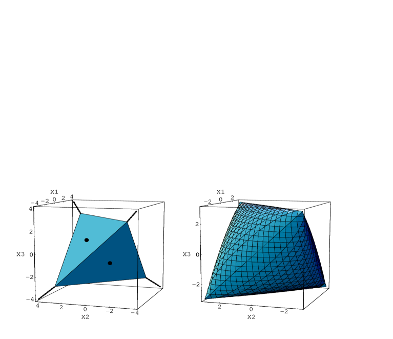
Figure 7: The fundamental domain (left) for constant gauge fields on $S^{3}$, with respect to the “instanton” framing $e_{\mu}^{a}$, in the diagonal representation $A_{a}=x_{a}\sigma_{a}$ (no sum over $a$). By the dots on the faces we indicate the sphalerons, whereas the dashed lines represent the symmetry axes of the tetrahedron. To the right we display the Gribov horizon, which encloses the fundamental domain, coinciding with it at the singular boundary points along the edges of the tetrahedron.

Numerical coefficients for $\mbox{$\cal V$}^{(1)}_{\rm efff}$ $\kappa_{1}$ = $-0$. $2453459985179565$ $\kappa_{2}$ = $3$. $66869179814223$ $\kappa_{3}$ = $0$. $500703203096610$ $\kappa_{4}$ = $-0$. $839359633413003$ $\kappa_{5}$ = $-0$. $849965412245339$ $\kappa_{6}$ = $-0$. $06550330854836428$ $\kappa_{7}$ = $-0$. $3617122159967145$ $\kappa_{8}$ = $-2$. $295356861354712$

An effective Hamiltonian for the $c$ and $d$ modes is derived from the one-loop effective action[34]. To lowest order it is given by

$$H=-\frac{g^{2}(R)}{4\pi^{2}R}\left(\left(\frac{\partial}{\partial c_{i}^{a}}\right)^{2}+\left(\frac{\partial}{\partial d_{i}^{a}}\right)^{2}\right)+\frac{1}{g^{2}(R)R}\mbox{$\cal V$}(c,d)+\frac{1}{R}\mbox{$\cal V$}^{(1)}_{\rm eff}(c,d),$$ (29)

where $g(R)$ is the running coupling constant (related to the MS running coupling by a finite renormalisation, such that kinetic term above has no corrections). The one-loop correction to the effective potential[34] is given by (for $\kappa_{i}$ see table 1):

$$\mbox{$\cal V$}^{(1)}_{\rm eff}(c,d) = \mbox{$\cal V$}^{(1)}_{\rm eff}(c)+\mbox{$\cal V$}^{(1)}_{\rm eff}(d)+\kappa_{7}(c^{a}_{i})^{2}(d^{b}_{j})^{2}+\kappa_{8}(c^{a}_{i}d^{a}_{j})^{2},$$ (30)

$$\mbox{$\cal V$}^{(1)}_{\rm eff}(c) = \kappa_{1}(c^{a}_{i})^{2}+\kappa_{2}\det c+\kappa_{3}(c^{a}_{i}c^{a}_{i})^{2}+\kappa_{4}(c^{a}_{i}c^{a}_{j})^{2}+\kappa_{5}(c^{a}_{i})^{2}\det c+\kappa_{6}(c^{a}_{i}c^{a}_{i})^{3}.$$

Errors due to an adiabatic approximation are not necessarily suppressed by powers of the coupling constant. Nevertheless, one expects to achieve an approximate understanding of the non-perturbative dynamics in this way[34].

The boundary conditions are chosen so as to coincide with the appropriate boundary conditions near the sphalerons, but such that the gauge and (left and right) rotational invariances are not destroyed. Projections on the irreducible representations of these symmetries turned out to be essential to reduce the size of the matrices to be diagonalised in a Rayleigh-Ritz analysis. Remarkably all this could be implemented in a tractable way[34]. Results are summarised in figure 8. One of the most important features is that the $0^{-}$ glueball is (slightly) lighter than the $0^{+}$ in perturbation theory, but when including the effects of the boundary of the fundamental domain, setting in at $f\equiv g^{2}/2\pi^{2}\sim 0.2$, the $0^{-}/0^{+}$ mass ratio rapidly increases. Beyond $f\sim 0.28$ it can be shown that the wave functionals start to feel parts of the boundary of the fundamental domain which the present calculation is not representing properly[34]. This value of $f$ corresponds to a circumference of roughly 1.3 fm, when setting the scale as for the torus, assuming the scalar glueball mass in both geometries at this intermediate volume to coincide.

Figure 8: The full one-loop results for the masses of scalar, tensor and odd glueballs on $S^{3}$ as a function of $f=g^{2}(R)/2\pi^{2}$ for $\theta=0$. The dashed lines correspond to the perturbative result.

5 DISCUSSION

We have analysed in detail the boundary of the fundamental domain for SU(2) gauge theories on the three-torus and three-sphere. It is important to note that it is necessary to divide $\cal A$ by the set of all gauge transformations, including those that are homotopically non-trivial, to get the physical configuration space. All the non-trivial topology is then retrieved by the identifications of points on the boundary of the fundamental domain.

As we already mentioned in the introduction, the knowledge of the boundary identifications is important in the case that the wave functionals spread out in configuration space to such an extent that they become sensitive to these identifications. This happens at large volumes, whereas at very small volumes the wave functional is localised around $A=0$ and one need not worry about these non-perturbative effects. That these effects can be dramatic, even at relatively small volumes (above a tenth of a fermi across), was demonstrated for the case of the torus. However, for that case the structure of the fundamental domain (restricted to the abelian zero-energy modes) is a hypercube and deviates considerably from the fundamental domain of the three-sphere. Nevertheless, the spectrum for the sphere is compatible with that for the torus in volumes around one fermi across[39], with $m(2^{+})/m(0^{+})\sim 1.5$ and $m(0^{-})/m(0^{+})\sim 1.7$.

It should be noted that the shape of $\Lambda$ is independent of $L$ if the gauge field is expressed in units of $1/L$. Suppose that the coupling constant will grow without bound. This would make the potential irrelevant and makes the wave functional spread out over the whole of field space (which could be seen as a strong coupling expansion). If the kinetic term would have been trivial the wave functionals would be “plane waves” on a space with complicated boundary conditions. In that case it seems unavoidable that the infinite volume limit would depend on the geometry (like $T^{3}$ or $S^{3}$) that is scaled-up to infinity. With the non-triviality of the kinetic term this conclusion cannot be readily made and our present understanding only allows comparison in volumes around one cubic fermi. However, one way to avoid this undesirable dependence on the geometry is that the vacuum is unstable against domain formation. As periodic subdivisions are space filling on a torus, this seems to be the preferred geometry to study domain formation. In a naive way it will give the correct string tension (flux conservation tells us to “string” the domains that carry electric flux) and tensor to scalar mass ratio (averaging over the orientations of the domains is expected to lead to a multiplicity weighted average of the $T_{2}$ and $E$ masses). Furthermore, the natural dislocations of such a domain picture are gauge dislocations. The point-like gauge dislocations in four dimensions are instantons and in three dimensions they are monopoles. Their density is expected to be given roughly as one per domain (with a volume of around 0.5 cubic fermi). Also the coupling constant will stop running at the scale of the domain size. We have discussed this elsewhere and refer the reader to refs.[6, 32, 40] for further details.

References

- [1] O. Babelon and C. Viallet, Comm.Math.Phys. 81:515 (1981).
- [2] V. Gribov, Nucl.Phys. B139:1 (1978).
- [3] I. Singer, Comm.Math.Phys. 60:7 (1978).
- [4] W. Nahm, in: “IV Warsaw Sym.Elem.Part.Phys,” 1981, Z.Ajduk, ed. (1981) p.275.
- [5] J. Koller and P. van Baal, Nucl. Phys. B302:1 (1988); P. van Baal, Acta Phys. Pol. B20:295 (1989).
- [6] P. van Baal, in: “Probabilistic Methods in Quantum Field Theory and Quantum Gravity,” ed. P.H. Damgaard e.a., Plenum Press, New York (1990) p31; Nucl.Phys. B(Proc.Suppl.)20:3 (1991).
- [7] M.A. Semenov-Tyan-Shanskii and V.A. Franke, Zapiski Nauchnykh Seminarov Leningradskogo Otdeleniya Matematicheskogo Instituta im. V.A. Steklov AN SSSR 120:159 (1982). Translation: Plenum Press, New York (1986) p.999.
- [8] N.M. Christ and T.D. Lee, Phys. Rev. D22:939 (1980).
- [9] M. Lüscher, Nucl. Phys. B219:233 (1983).
- [10] R.E. Cutkosky, J. Math. Phys. 25:939 (1984) 939; R.E. Cutkosky and K. Wang, Phys. Rev. D37:3024 (1988); R.E. Cutkosky, Czech. J. Phys. 40:252 (1990).
- [11] P. van Baal and N. D. Hari Dass, Nucl.Phys. B385:185 (1992).
- [12] P. van Baal, in: ”Non-perturbative approaches to Quantum Chromodynamics”, D. Diakonov, ed., Gatchina, 1995, pp.4-23.
- [13] G. Dell’Antonio and D. Zwanziger, in: “Probabilistic Methods in Quantum Field Theory and Quantum Gravity,” ed. P.H. Damgaard e.a., (Plenum Press, New York, 1990) p07; G. Dell’Antonio and D. Zwanziger, Comm. Math. Phys. 138:291 (1991).
- [14] G. Dell‘Antonio and D. Zwanziger, Nucl.Phys. B326:333 (1989).
- [15] D. Zwanziger, Nucl. Phys. B378:525 (1992).
- [16] P. van Baal, Nucl.Phys. B369:259 (1992).
- [17] S. Donaldson and P. Kronheimer, The geometry of four manifolds (Oxford University Press, 1990); D. Freed and K. Uhlenbeck, Instantons and four-manifolds, M.S.R.I. publ. Vol. I (Springer, New York, 1984).
- [18] P. van Baal, in: Proceedings of the International Symposium on Advanced Topics of Quantum Physics, eds. J.Q. Liang, e.a., Science Press (Beijing, 1993), p.133, hep-lat/9207029.
- [19] P. van Baal and B. van den Heuvel, Nucl.Phys. B417:215 (1994).
- [20] G. ’t Hooft, Nucl. Phys. B153:141 (1979).
- [21] P. van Baal and J. Koller, Ann. Phys. (N.Y.) 174:299 (1987).
- [22] G. ’t Hooft, Phys.Rev. D14:3432 (1976).
- [23] C. Bloch, Nucl. Phys. 6:329 (1958).
- [24] C. Vohwinkel, Phys. Lett. B213:54 (1988).
- [25] P. van Baal, Phys. Lett. 224B:397 (1989); Nucl.Phys. B(Proc.Suppl)17:581 (1990); Nucl. Phys. B351:183 (1991).
- [26] C. Michael, G.A. Tickle and M.J. Teper, Phys. Lett. 207B:313 (1988); C. Michael, Nucl. Phys. B329:225 (1990).
- [27] M. Lüscher and G. Münster, Nucl. Phys. B232:445 (1984).
- [28] C. Vohwinkel, Phys. Rev. Lett. 63:2544 (1989).
- [29] M. García Pérez and P. van Baal, Nucl. Phys. B429:451 (1994).
- [30] M. García Pérez, A. González-Arroyo, J. Snippe and P. van Baal, Nucl. Phys. B413:535 (1994); Nucl. Phys. B(Proc.Suppl)34:222 (1994).
- [31] P. van Baal, Nucl. Phys. B(Proc.Suppl)49:238 (1996), hep-th/9512223.
- [32] P. van Baal, The QCD vacuum, review at Lattice’97 (Edinburgh, 22-26 July 1996), hep-lat/9709066.
- [33] Y. Hosotani, Phys. Lett. 147B:44 (1984).
- [34] B.M van den Heuvel, Nucl. Phys. B(Proc.Suppl.)42:823 (1995); Phys. Lett. B368:124 (1996); B386:233 (1996); Nucl. Phys. B488:282 (1997).
- [35] M. Lüscher, Phys. Lett. B70:321 (1977).
- [36] A. Belavin, A. Polyakov, A. Schwarz and Y. Tyupkin, Phys. Lett. 59B:85 (1975); M. Atiyah, V. Drinfeld, N. Hitchin and Yu. Manin, Phys. Lett. 65A:185 (1978).
- [37] F. R. Klinkhamer and M. Manton, Phys. Rev. D30:2212 (1984).
- [38] P. van Baal and R.E. Cutkosky, Int. J. Mod. Phys. A(Proc. Suppl.)3A:323 (1993).
- [39] C. Michael and M. Teper, Phys.Lett. B199:95 (1987).
- [40] J. Koller and P. van Baal, Nucl. Phys. B(Proc.Suppl)4:47 (1988).