LIGHT-FRONT QCD: A CONSTITUENT PICTURE OF HADRONS

Department of Physics, The Ohio State University
Columbus, Ohio, 43210, USA

MOTIVATION AND STRATEGY

We seek to derive the structure of hadrons from the fundamental theory of the strong interaction, QCD. Our work is founded on the hypothesis that a constituent approximation can be derived from QCD, so that a relatively small number of quark and gluon degrees of freedom need be explicitly included in the state vectors for low-lying hadrons.${}^{\hbox{\scriptsize\cite[cite]{[\@@bibref{}{nonpert}{}{}]}}}$ To obtain a constituent picture, we use a Hamiltonian approach in light-front coordinates.${}^{\hbox{\scriptsize\cite[cite]{[\@@bibref{}{dirac}{}{}]}}}$

I do not believe that light-front Hamiltonian field theory is extremely useful for the study of low energy QCD unless a constituent approximation can be made, and I do not believe such an approximation is possible unless cutoffs that it violate manifest gauge invariance and covariance are employed. Such cutoffs inevitably lead to relevant and marginal effective interactions (i.e., counterterms) that contain functions of longitudinal momenta.${}^{\hbox{\scriptsize\cite[cite]{[\@@bibref{}{coupcoh,perryrg}{}{}]}}}$ It is it not possible to renormalize light-front Hamiltonians in any useful manner without developing a renormalization procedure that can produce these non-canonical counterterms.

The line of investigation I discuss has been developed by a small group of theorists who are working or have worked at Ohio State University and Warsaw University.${}^{\hbox{\scriptsize 1,3-19}}$ Ken Wilson provided the initial impetus for this work, and at a very early stage outlined much of the basic strategy we employ.${}^{\hbox{\scriptsize\cite[cite]{[\@@bibref{}{wilson90}{}{}]}}}$

I make no attempt to provide enough details to allow the reader to start doing light-front calculations. The introductory article by Harindranath${}^{\hbox{\scriptsize\cite[cite]{[\@@bibref{}{hari96a}{}{}]}}}$ is helpful in this regard. An earlier version of these lectures${}^{\hbox{\scriptsize\cite[cite]{[\@@bibref{}{brazil}{}{}]}}}$ also provides many more details.

A Constituent Approximation Depends on Tailored Renormalization

If it is possible to derive a constituent approximation from QCD, we can formulate the hadronic bound state problem as a set of coupled few-body problems. We obtain the states and eigenvalues by solving

$$H_{\Lambda}\mid\Psi_{\Lambda}\rangle=E\mid\Psi_{\Lambda}\rangle,$$ (1)

where,

$$\mid\Psi_{\Lambda}\rangle=\phi^{\Lambda}_{q\bar{q}}\mid q\bar{q}\rangle+\phi^{\Lambda}_{q\bar{q}g}\mid q\bar{q}g\rangle+\cdot\cdot\cdot.$$ (2)

where I use shorthand notation for the Fock space components of the state. The full state vector includes an infinite number of components, and in a constituent approximation we truncate this series. We derive the Hamiltonian from QCD, so we must allow for the possibility of constituent gluons. I have indicated that the Hamiltonian and the state both depend on a cutoff, $\Lambda$, which is critical for the approximation.

This approach has no chance of working without a renormalization scheme tailored to it. Much of our work has focused on the development of such a renormalization scheme.${}^{\hbox{\scriptsize 3,4,17-19}}$ In order to understand the constraints that have driven this development, seriously consider under what conditions it might be possible to truncate the above series without making an arbitrarily large error in the eigenvalue. I focus on the eigenvalue, because it will certainly not be possible to approximate all observable properties of hadrons (e.g., wee parton structure functions) this way.

For this approximation to be valid, all many-body states must approximately decouple from the dominant few-body components. We know that even in perturbation theory, high energy many-body states do not simply decouple from few-body states. In fact, the errors from simply discarding high energy states are infinite. In second-order perturbation theory, for example, high energy photons contribute an arbitrarily large shift to the mass of an electron. This second-order effect is illustrated in Figure 1, and the precise interpretation for this light-front time-ordered diagram will be given below. The solution to this problem is well-known, renormalization. We must use renormalization to move the effects of high energy components in the state to effective interactions in the Hamiltonian.

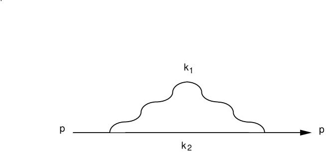
Figure 1.: The second-order shift in the self-energy of a bare electron due to mixing with electron-photon states.

It is difficult to see how a constituent approximation can emerge using any regularization scheme that does not employ a cutoff that either removes degrees of freedom or removes direct couplings between degrees of freedom. A Pauli-Villars “cutoff,” for example, drastically increases the size of Fock space and destroys the hermiticity of the Hamiltonian.

In the best case scenario we expect the cutoff to act like a resolution. If the cutoff is increased to an arbitrarily large value, the resolution increases and instead of seeing a few constituents we resolve the substructure of the constituents and the few-body approximation breaks down. As the cutoff is lowered, this substructure is removed from the state vectors, and the renormalization procedure replaces it with effective interactions in the Hamiltonian. Any “cutoff” that does not remove this substructure from the states is of no use to us.

This point is well-illustrated by the QED calculations discussed below${}^{\hbox{\scriptsize\cite[cite]{[\@@bibref{}{brazil,BJ97a,BJ97c}{}{}]}}}$$\!.$ There is a window into which the cutoff must be lowered for the constituent approximation to work. If the cutoff is too large, atomic states must explicitly include photons. After the cutoff is lowered to a value that can be self-consistently determined a-posteriori, photons are removed from the states and replaced by the Coulomb interaction and relativistic corrections. The cutoff cannot be lowered too far using a perturbative renormalization group, hence the window.

Thus, if we remove high energy degrees of freedom, or coupling to high energy degrees of freedom, we should encounter self-energy shifts leading to effective one-body operators, vertex corrections leading to effective vertices, and exchange effects leading to explicit many-body interactions not found in the canonical Hamiltonian. We naively expect these operators to be local when acting on low energy states, because simple uncertainty principle arguments indicate that high energy virtual particles cannot propagate very far. Unfortunately this expectation is indeed naive, and at best we can hope to maintain transverse locality.${}^{\hbox{\scriptsize\cite[cite]{[\@@bibref{}{perryrg}{}{}]}}}$ I will elaborate on this point below. The study of perturbation theory with the cutoffs we must employ makes it clear that it is not enough to adjust the canonical couplings and masses to renormalize the theory. It is not possible to make significant progress towards solving light-front QCD without fully appreciating this point.

Low energy many-body states do not typically decouple from low energy few-body states. The worst of these low energy many-body states is the vacuum. This is what drives us to use light-front coordinates.${}^{\hbox{\scriptsize\cite[cite]{[\@@bibref{}{dirac}{}{}]}}}$ Figure 2 shows a pair of particles being produced out of the vacuum in equal-time coordinates $t$ and $z$. The transverse components $x$ and $y$ are not shown, because they are the same in equal-time and light-front coordinates. The figure also shows light-front time,

$$x^{+}=t+z\;,$$ (3)

and the light-front longitudinal spatial coordinate,

$$x^{-}=t-z\;.$$ (4)

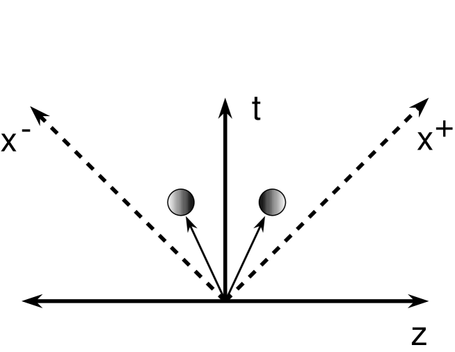
Figure 2.: Light-front coordinates. Light-front ‘time’ is $x^{+}=t+z$, and the light-front longitudinal spatial coordinate is $x^{-}=t-z$.

In equal-time coordinates it is kinematically possible for virtual pairs to be produced from the vacuum (although relevant interactions actually produce three or more particles from the vacuum), as long as their momenta sum to zero so that three-momentum is conserved. Because of this, the state vector for a proton includes an arbitrarily large number of particles that are disconnected from the proton. The only constraint imposed by relativity is that particle velocities be less than or equal to that of light.

In light-front coordinates, however, we see that all allowed trajectories lie in the first quadrant. In other words, light-front longitudinal momentum, $p^{+}$ (conjugate to $x^{-}$ since $a\cdot b={\scriptstyle{{1\over 2}}}(a^{+}b^{-}+a^{-}b^{+})-{\bf a}_{\perp}\cdot{\bf b}_{\perp}$), is always positive,

$$p^{+}\geq 0\;.$$ (5)

We exclude $p^{+}=0$, forcing the vacuum to be trivial because it is the only state with $p^{+}=0$. Moreover, the light-front energy of a free particle of mass $m$ is

$$p^{-}={{\bf p}_{\perp}^{2}+m^{2}\over p^{+}}\;.$$ (6)

This implies that all free particles with zero longitudinal momentum have infinite energy, unless their mass and transverse momentum are identically zero. Replacing such particles with effective interactions should be reasonable.

• Is the vacuum really trivial?

• What about confinement?

• What about chiral symmetry breaking?

• What about instantons?

• What about the job security of theorists who study the vacuum?

The question of how one should treat “zero modes,” degrees of freedom (which may be constrained) with identically zero longitudinal momentum, divides the light-front community. Our attitude is that explicitly including zero modes defeats the purpose of using light-front coordinates, and we do not believe that significant progress will be made in this direction, at least not in $3+1$ dimensions.

The vacuum in our formalism is trivial. We are forced to work in the “hidden symmetry phase” of the theory, and to introduce effective interactions that reproduce all effects associated with the vacuum in other formalisms.${}^{\hbox{\scriptsize\cite[cite]{[\@@bibref{}{nonpert,burkardt93,burkardt97}{}{}]}}}$ The simplest example of this approach is provided by a scalar field theory with spontaneous symmetry breaking. It is possible to shift the scalar field and deal explicitly with a theory containing symmetry breaking interactions. In the simplest case $\phi^{3}$ is the only relevant or marginal symmetry breaking interaction, and one can simply tune this coupling to the value corresponding to spontaneous rather than explicit symmetry breaking. Ken Wilson and I have also shown that in such simple cases one can use coupling coherence to fix the strength of this interaction so that tuning is not required.${}^{\hbox{\scriptsize\cite[cite]{[\@@bibref{}{coupcoh}{}{}]}}}$

I will make an additional drastic assumption in these lectures, an assumption that Ken Wilson does not believe will hold true. I will assume that all effective interactions we require are local in the transverse direction. If this is true, there are a finite number of relevant and marginal operators, although each contains a function of longitudinal momenta that must be determined by the renormalization procedure. There are many more relevant and marginal operators in the renormalized light-front Hamiltonian than in ${\cal L}_{\rm QCD}$. If transverse locality is violated, the situation is much worse than this.

The presence of extra relevant and marginal operators that contain functions tremendously complicates the renormalization problem, and a common reaction to this problem is denial, which may persist for years. However, this situation may make possible tremendous simplifications in the final nonperturbative problem. For example, few-body operators must produce confinement manifestly!

Confinement cannot require particle creation and annihilation, flux tubes, etc. This is easily seen using a variational argument. Consider a color neutral quark-antiquark pair that are separated by a distance $R$, which is slowly increased to infinity. Moreover, to see the simplest form of confinement assume that there are no light quarks, so that the energy should increase indefinitely as they are separated if the theory possesses confinement. At each separation the gluon components of the state adjust themselves to minimize the energy. But this means that the expectation value of the Hamiltonian for a state with no gluons must exceed the energy of the state with gluons, and therefore must diverge even more rapidly than the energy of the true ground state. This means that there must be a two-body confining interaction in the Hamiltonian. If the renormalization procedure is unable to produce such confining two-body interactions, the constituent picture will not arise.

Manifest gauge invariance and manifest rotational invariance require all physical states to contain an arbitrarily large number of constituents. Gauge invariance is not manifest since we work in light-cone gauge with the zero modes removed; and it is easy to see that manifest rotational invariance requires an infinite number of constituents. Rotations about transverse axes are generated by dynamic operators in interacting light-front field theories, operators that create and annihilate particles.${}^{\hbox{\scriptsize\cite[cite]{[\@@bibref{}{dirac,chaone}{}{}]}}}$ No state with a finite number of constituents rotates into itself or transforms as a simple tensor under the action of such generators. These symmetries seem to imply that we can not obtain a constituent approximation.

To cut this Gordian knot we employ cutoffs that violate gauge invariance and covariance, symmetries which then must be restored by effective interactions, and which need not be restored exactly. A familiar example of this approach is supplied by lattice gauge theory, where rotational invariance is violated by the lattice.

Simple Strategy

We have recently employed a conceptually simple strategy to complete bound state calculations. The first step is to use a perturbative similarity renormalization group${}^{\hbox{\scriptsize\cite[cite]{[\@@bibref{}{glazek1,glazek2,Gl97a}{}{}]}}}$ and coupling coherence${}^{\hbox{\scriptsize\cite[cite]{[\@@bibref{}{coupcoh,perryrg}{}{}]}}}$ to find the renormalized Hamiltonian as an expansion in powers of the canonical coupling:

$$H^{\Lambda}=h_{0}+g_{\Lambda}h_{1}^{\Lambda}+g_{\Lambda}^{2}h_{2}^{\Lambda}+\cdot\cdot\cdot$$ (7)

We compute this series to a finite order, and to date have not required any ad hoc assumptions to uniquely fix the Hamiltonian. No operators are added to the hamiltonian, so the hamiltonian is completely determined by the underlying theory to this order.

The second step is to employ bound state perturbation theory to solve the eigenvalue problem. The complete Hamiltonian contains every interaction (although each is cut off) contained in the canonical Hamiltonian, and many more. We separate the Hamiltonian,

$$H^{\Lambda}=H_{0}^{\Lambda}+V^{\Lambda}\;,$$ (8)

treating $H_{0}^{\Lambda}$ nonperturbatively and computing the effects of $V^{\Lambda}$ in bound state perturbation theory. We must choose $H_{0}^{\Lambda}$ and $\Lambda$ so that $H_{0}^{\Lambda}$ is manageable and to minimize corrections from higher orders of $V^{\Lambda}$ within a constituent approximation.

If a constituent approximation is valid after $\Lambda$ is lowered to a critical value which must be determined, we may be able to move all creation and annihilation operators to $V^{\Lambda}$. $H_{0}^{\Lambda}$ will include many-body interactions that do not change particle number, and these interactions should be primarily responsible for the constituent bound state structure.

There are several obvious flaws in this strategy. Chiral symmetry-breaking operators, which must be included in the Hamiltonian since we work entirely in the hidden symmetry phase of the theory, do not appear at any finite order in the coupling. These operators must simply be added and tuned to fit spectra or fixed by a non-perturbative renormalization procedure.${}^{\hbox{\scriptsize\cite[cite]{[\@@bibref{}{nonpert,mustaki,Br94b}{}{}]}}}$ In addition, there are perturbative errors in the strengths of all operators that do appear. We know from simple scaling arguments${}^{\hbox{\scriptsize\cite[cite]{[\@@bibref{}{wilson75}{}{}]}}}$ that when $\Lambda$ is in the scaling regime:

• small errors in relevant operators exponentiate in the output,

• small errors in marginal operators produce comparable errors in output,

• small errors in irrelevant operators tend to decrease exponentially in the output.

This means that even if a relevant operator appears (e.g., a constituent quark or gluon mass operator), we may need to tune its strength to obtain reasonable results. We have not had to do this, but we have recently studied some of the effects of tuning a gluon mass operator.${}^{\hbox{\scriptsize\cite[cite]{[\@@bibref{}{Sz97a}{}{}]}}}$

To date this strategy has produced well-known results in QED${}^{\hbox{\scriptsize\cite[cite]{[\@@bibref{}{brazil,BJ97a,BJ97c}{}{}]}}}$ through the Lamb shift, and reasonable results for heavy quark bound states in QCD.${}^{\hbox{\scriptsize\cite[cite]{[\@@bibref{}{brazil,Br96a,Br97a,Sz97a}{}{}]}}}$ The primary objective of the remainder of these lectures is to review these results. I first use the Schwinger model as an illustration of a light-front bound state calculation. This model does not require renormalization, so before turning to QED and QCD I discuss the renormalization procedure that we have developed.

LIGHT-FRONT SCHWINGER MODEL

In this section I use the Schwinger model, massless QED in $1+1$ dimensions, to illustrate the basic strategy we employ after we have computed the renormalized Hamiltonian. No model in $1+1$ dimensions illustrates the renormalization problems we must solve before we can start to study QCD₃₊₁.

The Schwinger model can be solved analytically.${}^{\hbox{\scriptsize\cite[cite]{[\@@bibref{}{schwing, lowenstein}{}{}]}}}$ Charged particles are confined because the Coulomb interaction is linear and there is only one physical particle, a massive neutral scalar particle with no self-interactions. The Fock space content of the physical states depends crucially on the coordinate system and gauge, and it is only in light-front coordinates that a simple constituent picture emerges.${}^{\hbox{\scriptsize\cite[cite]{[\@@bibref{}{bergknoff}{}{}]}}}$

The Schwinger model was first studied in Hamiltonian light-front field theory by Bergknoff.${}^{\hbox{\scriptsize\cite[cite]{[\@@bibref{}{bergknoff}{}{}]}}}$ My description of the model follows his closely, and I recommend his paper to the reader. Bergknoff showed that the physical boson in the light-front massless Schwinger model in light-cone gauge is a pure electron-positron state. This is an amazing result in a strong-coupling theory of massless bare particles, and it illustrates how a constituent picture may arise in QCD. The electron-positron pair is confined by the linear Coulomb potential. The light-front kinetic energy vanishes in the massless limit, and the potential energy is minimized by a wave function that is flat in momentum space, as one might expect since a linear potential produces a state that is as localized as possible (given kinematic constraints due to the finite velocity of light) in position space.

In order to solve this theory I must first set up a large number of details. I recommend that for a first reading these details be skimmed, because the general idea is more important than the detailed manipulations. The Lagrangian for the theory is

$${\cal L}=\overline{\psi}\bigl{(}i\not{{\hskip-2.27626pt}\partial}-m\bigr{)}\psi-e\overline{\psi}\gamma_{\mu}\psi A^{\mu}-{1\over 4}F_{\mu\nu}F^{\mu\nu}\;,$$ (9)

where $F_{\mu\nu}$ is the electromagnetic field strength tensor. I have included an electron mass, $m$, which is taken to zero later. I choose light-cone gauge,

$$A^{+}=0\;.$$ (10)

In this gauge we avoid ghosts, so that the Fock space has a positive norm. This is absolutely essential if we want to apply intuitive techniques from many-body quantum mechanics.

Many calculations are simplified by the use of a chiral representation of the Dirac gamma matrices, so in this section I will use:

$$\gamma^{0}=\left(\begin{array}[]{cc}0&-i\\ i&0\end{array}\right)~{}~{},~{}~{}~{}\gamma^{1}=\left(\begin{array}[]{cc}0&i\\ i&0\end{array}\right)\;,$$ (11)

which leads to the light-front coordinate gamma matrices,

$$\gamma^{+}=\left(\begin{array}[]{cc}0&0\\ 2i&0\end{array}\right)~{}~{},~{}~{}~{}\gamma^{-}=\left(\begin{array}[]{cc}0&-2i\\ 0&0\end{array}\right)\;.$$ (12)

In light-front coordinates the fermion field $\psi$ contains only one dynamical degree of freedom, rather than two. To see this, first define the projection operators,

$$\Lambda_{+}={1\over 2}\gamma^{0}\gamma^{+}=\left(\begin{array}[]{cc}1&0\\ 0&0\end{array}\right)~{}~{}~{}~{}~{}\Lambda_{-}={1\over 2}\gamma^{0}\gamma^{-}=\left(\begin{array}[]{cc}0&0\\ 0&1\end{array}\right)\;.$$ (13)

Using these operators split the fermion field into two components,

$$\psi=\psi_{+}+\psi_{-}=\Lambda_{+}\psi+\Lambda_{-}\psi\;.$$ (14)

The two-component Dirac equation in this gauge is

$$\biggl{(}{i\over 2}\gamma^{+}\partial^{-}+{i\over 2}\gamma^{-}\partial^{+}-m-{e\over 2}\gamma^{+}A^{-}\biggr{)}\psi=0\;;$$ (15)

which can be split into two one-component equations,

$$i\partial^{-}{\tilde{\psi}}_{+}=-im{\tilde{\psi}}_{-}+eA^{-}{\tilde{\psi}}_{+}\;,$$ (16)

$$i\partial^{+}{\tilde{\psi}}_{-}=im{\tilde{\psi}}_{+}\;.$$ (17)

Here ${\tilde{\psi}}_{\pm}$ refers to the non-zero component of $\psi_{\pm}$.

The equation for $\psi_{+}$ involves the light-front time derivative, $\partial^{-}$; so $\psi_{+}$ is a dynamical degree of freedom that must be quantized. On the other hand, the equation for $\psi_{-}$ involves only spatial derivatives, so $\psi_{-}$ is a constrained degree of freedom that should be eliminated in favor of $\psi_{+}$. Formally,

$${\tilde{\psi}}_{-}={m\over\partial^{+}}{\tilde{\psi}}_{+}\;.$$ (18)

This equation is not well-defined until boundary conditions are specified so that $\partial^{+}$ can be inverted. I will eventually define this operator in momentum space using a cutoff, but I want to delay the introduction of a cutoff until a calculation requires it.

I have chosen the gauge so that $A^{+}=0$, and the equation for $A^{-}$ is

$$-{1\over 4}\bigl{(}\partial^{+}\bigr{)}^{2}A^{-}=e\psi_{+}^{\dagger}\psi_{+}\;.$$ (19)

$A^{-}$ is also a constrained degree of freedom, and we can formally eliminate it,

$$A^{-}=-{4e\over\bigl{(}\partial^{+}\bigr{)}^{2}}\psi_{+}^{\dagger}\psi_{+}\;.$$ (20)

We are now left with a single dynamical degree of freedom, $\psi_{+}$, which we can quantize at $x^{+}=0$,

$$\bigl{\{}\psi_{+}(x^{-}),\psi_{+}^{\dagger}(y^{-})\bigr{\}}=\Lambda_{+}\delta(x^{-}-y^{-})\;.$$ (21)

We can introduce free particle creation and annihilation operators and expand the field operator at $x^{+}=0$,

$${\tilde{\psi}}_{+}(x^{-})=\int_{k^{+}>0}{dk^{+}\over 4\pi}\Biggl{[}b_{k}e^{-ik\cdot x}+d_{k}^{\dagger}e^{ik\cdot x}\Biggr{]}\;,$$ (22)

with,

$$\bigl{\{}b_{k},b_{p}^{\dagger}\}=4\pi\delta(k^{+}-p^{+})\;.$$ (23)

In order to simplify notation, I will often write $k$ to mean $k^{+}$. If I need $k^{-}=m^{2}/k^{+}$, I will provide the superscript.

The next step is to formally specify the Hamiltonian. I start with the canonical Hamiltonian,

$$H=\int dx^{-}\Bigl{(}H_{0}+V\Bigr{)}\;,$$ (24)

$$H_{0}=\psi_{+}^{\dagger}\Biggl{(}{m^{2}\over i\partial^{+}}\Biggr{)}\psi_{+}\;,$$ (25)

$$V=-2e^{2}\psi_{+}^{\dagger}\psi_{+}\Biggl{(}{1\over\partial^{+}}\Biggr{)}^{2}\psi_{+}^{\dagger}\psi_{+}\;.$$ (26)

To actually calculate:

• replace $\psi_{+}$ with its expansion in terms of $b_{k}$ and $d_{k}$,

• normal-order,

• throw away constants,

• drop all operators that require $b_{0}$ and $d_{0}$.

The free part of the Hamiltonian becomes

$$H_{0}=\int_{k>0}{dk\over 4\pi}\Biggl{(}{m^{2}\over k}\Biggr{)}\bigl{(}b_{k}^{\dagger}b_{k}+d_{k}^{\dagger}d_{k}\bigr{)}\;.$$ (27)

When $V$ is normal-ordered, we encounter new one-body operators,

$$H^{\prime}_{0}={e^{2}\over 2\pi}\int_{k>0}{dk\over 4\pi}\Biggl{[}\int_{p>0}dp\biggl{(}{1\over(k-p)^{2}}-{1\over(k+p)^{2}}\biggr{)}\Biggr{]}\bigl{(}b_{k}^{\dagger}b_{k}+d_{k}^{\dagger}d_{k}\bigr{)}\;.$$ (28)

This operator contains a divergent momentum integral. From a mathematical point of view we have been sloppy and need to carefully add boundary conditions and define how $\partial^{+}$ is inverted. However, I want to apply physical intuition and even though no physical photon has been exchanged to produce the initial interaction, I will act as if a photon has been exchanged and everywhere an ‘instantaneous photon exchange’ occurs I will cut off the momentum. In the above integral I insist,

$$|k-p|>\epsilon\;.$$ (29)

Using this cutoff we find that

$$H^{\prime}_{0}={e^{2}\over\pi}\int{dk\over 4\pi}\biggl{(}{1\over\epsilon}-{1\over k}+{\cal O}(\epsilon)\biggr{)}\bigl{(}b_{k}^{\dagger}b_{k}+d_{k}^{\dagger}d_{k}\bigr{)}\;.$$ (30)

Comparing this result with the original free Hamiltonian, we see that a divergent mass-like term appears; but it does not have the same dispersion relation as the bare mass. Instead of depending on the inverse momentum of the fermion, it depends on the inverse momentum cutoff, which cannot appear in any physical result. There is also a finite shift in the bare mass, with the standard dispersion relation.

The normal-ordered interactions are

$$V^{\prime}=2e^{2}\int{dk_{1}\over 4\pi}\cdot\cdot\cdot{dk_{4}\over 4\pi}4\pi\delta(k_{1}+k_{2}-k_{3}-k_{4})$$

$$~{}~{}~{}~{}~{}~{}~{}~{}~{}~{}~{}\Biggl{\{}-{2\over(k_{1}-k_{3})^{2}}b_{1}^{\dagger}d_{2}^{\dagger}d_{4}b_{3}+{2\over(k_{1}+k_{2})^{2}}b_{1}^{\dagger}d_{2}^{\dagger}d_{3}b_{4}$$

$$~{}~{}~{}~{}~{}~{}~{}~{}~{}~{}~{}~{}~{}~{}-{1\over(k_{1}-k_{3})^{2}}\bigl{(}b_{1}^{\dagger}b_{2}^{\dagger}b_{3}b_{4}+d_{1}^{\dagger}d_{2}^{\dagger}d_{3}d_{4}\bigr{)}+\cdot\cdot\cdot\Biggr{\}}\;.$$ (31)

I do not display the interactions that involve the creation or annihilation of electron/positron pairs, which are important for the study of multiple boson eigenstates.

The first term in $V^{\prime}$ is the electron-positron interaction. The longitudinal momentum cutoff I introduced above requires $|k_{1}-k_{3}|>\epsilon$, so in position space we encounter a potential which I will naively define with a Fourier transform that ignores the fact that the momentum transfer cannot exceed the momentum of the state,

$$v(x^{-}) = 4q_{1}q_{2}\int_{-\infty}^{\infty}{dk\over 4\pi}\;{1\over k^{2}}\;\theta(|k|-\epsilon)\;{\rm exp}\bigl{(}-{i\over 2}kx^{-}\bigr{)}$$ (32)

$$= {q_{1}q_{2}\over\pi}\;\Biggl{[}{2\over\epsilon}-{\pi\over 2}|x^{-}|+{\cal O}(\epsilon)\Biggr{]}\;.$$

This potential contains a linear Coulomb potential that we expect in two dimensions, but it also contains a divergent constant that is negative for unlike charges and positive for like charges.

In charge neutral states the infinite constant in $V^{\prime}$ is exactly canceled by the divergent ‘mass’ term in $H^{\prime}_{0}$. This Hamiltonian assigns an infinite energy to states with net charge, and a finite energy as $\epsilon\rightarrow 0$ to charge zero states. This does not imply that charged particles are confined, but the linear potential prevents charged particles from moving to arbitrarily large separation except as charge neutral states. The confinement mechanism I propose for QCD in 3+1 dimensions shares many features with this interaction.

I would also like to mention that even though the interaction between charges is long-ranged, there are no van der Waals forces in 1+1 dimensions. It is a simple geometrical calculation to show that all long range forces between two neutral states cancel exactly. This does not happen in higher dimensions, and if we use long-range two-body operators to implement confinement we must also find many-body operators that cancel the strong long-range van der Waals interactions.

Given the complete Hamiltonian in normal-ordered form we can study bound states. A powerful tool for the initial study of bound states is the variational wave function. In this case, we can begin with a state that contains a single electron-positron pair,

$$|\Psi(P)\rangle=\int_{0}^{P}{dp\over 4\pi}\phi(p)b_{p}^{\dagger}d_{P-p}^{\dagger}|0\rangle\;.$$ (33)

The norm of this state is

$$\langle\Psi(P^{\prime})|\Psi(P)\rangle=4\pi P\delta(P^{\prime}-P)\Biggl{\{}{1\over P}\int_{0}^{P}{dp\over 4\pi}|\phi(p)|^{2}\Biggr{\}}\;,$$ (34)

where the factors outside the brackets provide a covariant plane wave normalization for the center-of-mass motion of the bound state, and the bracketed term should be set to one.

The expectation value of the one-body operators in the Hamiltonian is

$$\langle\Psi|H_{0}+H^{\prime}_{0}|\Psi\rangle={1\over P}\int{dk\over 4\pi}\Biggl{[}{m^{2}-e^{2}/\pi\over k}+{m^{2}-e^{2}/\pi\over P-k}+{2e^{2}\over\pi\epsilon}\Biggr{]}|\phi(k)|^{2}\;,$$ (35)

and the expectation value of the normal-ordered interactions is

$$\langle\Psi|V^{\prime}|\Psi\rangle=-{4e^{2}\over P}\int^{\prime}{dk_{1}\over 4\pi}{dk_{2}\over 4\pi}\Bigl{[}{1\over(k_{1}-k_{2})^{2}}-{1\over P^{2}}\Biggr{]}\phi^{*}(k_{1})\phi(k_{2})\;,$$ (36)

where I have dropped the overall plane wave norm. The prime on the last integral indicates that the range of integration in which $|k_{1}-k_{2}|<\epsilon$ must be removed. By expanding the integrand about $k_{1}=k_{2}$, one can easily confirm that the $1/\epsilon$ divergences cancel.

With $m=0$ the energy is minimized when

$$\phi(k)=\sqrt{4\pi}\;,$$ (37)

and the invariant-mass is

$$M^{2}={e^{2}\over\pi}\;.$$ (38)

This type of simple analysis can be used to show that this electron-positron state is actually the exact ground state of the theory with momentum $P$, and that bound states do not interact with one another.

The primary purpose of introducing the Schwinger model is to illustrate that bound state center-of-mass motion is easily separated from relative motion in light-front coordinates, and that standard quantum mechanical techniques can be used to analyze the relative motion of charged particles once the Hamiltonian is found. It is intriguing that even when the fermion is massless, the states are constituent states in light-cone gauge and in light-front coordinates. This is not true in other gauges and coordinate systems. The success of light-front field theory in 1+1 dimensions can certainly be downplayed, but it should be emphasized that no other method on the market is as powerful for bound state problems in 1+1 dimensions.

The most significant barriers to using light-front field theory to solve low energy QCD are not encountered in 1+1 dimensions. The Schwinger model is super-renormalizable, so we completely avoid serious ultraviolet divergences. There are no transverse directions, and we are not forced to introduce a cutoff that violates rotational invariance, because there are no rotations. Confinement results from the Coulomb interaction, and chiral symmetry is not spontaneously broken. This simplicity disappears in realistic $3+1$-dimensional calculations, which is one reason there are so few $3+1$-dimensional light-front field theory calculations.

LIGHT-FRONT RENORMALIZATION GROUP: SIMILARITY TRANSFORMATION AND COUPLING COHERENCE

As argued above, in $3+1$ dimensions we must introduce a cutoff on energies, $\Lambda$, and we never perform explicit bound state calculations with $\Lambda$ anywhere near its continuum limit. In fact, we want to let $\Lambda$ become as small as possible. In my opinion, any strategy for solving light-front QCD that requires the cutoff to explicitly approach infinity in the nonperturbative part of the calculation is useless. Therefore, we must set up and solve

$$P^{-}_{\Lambda}\mid\Psi_{\Lambda}(P)\rangle={{\bf P}_{\perp}^{2}+M^{2}\over P^{+}}\mid\Psi_{\Lambda}(P)\rangle\;.$$ (39)

Physical results, such as the mass, $M$, can not depend on the arbitrary cutoff, $\Lambda$, even as $\Lambda$ approaches the scale of interest. This means that $P^{-}_{\Lambda}$ and $\mid\Psi_{\Lambda}\rangle$ must depend on the cutoff in such a way that $\langle\Psi_{\Lambda}\mid P^{-}_{\Lambda}\mid\Psi_{\Lambda}\rangle$ does not. Wilson based the derivation of his renormalization group on this observation,${}^{\hbox{\scriptsize\cite[cite]{[\@@bibref{}{wilson65,wilson70,wilson74,wilson75}{}{}]}}}$ and we use Wilson’s renormalization group to compute $P^{-}_{\Lambda}$.

It is difficult to even talk about how the Hamiltonian depends on the cutoff without having a means of changing the cutoff. If we can change the cutoff, we can explicitly watch the Hamiltonian’s cutoff dependence change and fix its cutoff dependence by insisting that this change satisfy certain requirements (e.g., that the limit in which the cutoff is taken to infinity exists). We introduce an operator that changes the cutoff,

$$H(\Lambda_{1})=T[H(\Lambda_{0})]\;,$$ (40)

where I assume that $\Lambda_{1}<\Lambda_{0}$. To simplify the notation, I will let $H(\Lambda_{l})=H_{l}$. To renormalize the hamiltonian we study the properties of the transformation.

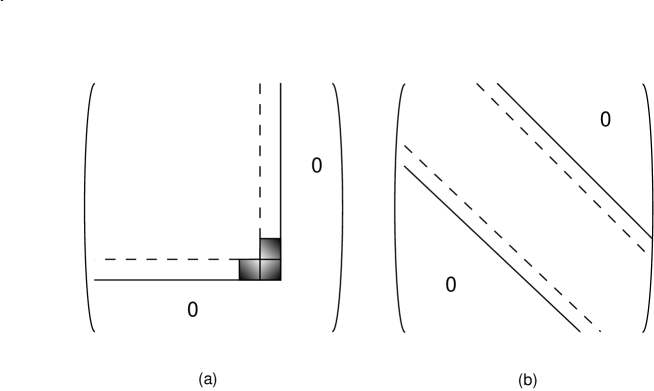
Figure 3.: Two ways to run a cutoff on free energy. In (a) a cutoff on the magnitude of the energy is lowered from the solid to the dashed lines, with problems resulting from the removed shaded region. In (b) a cutoff on how far off diagonal matrix elements appear is lowered from the dashed to the solid lines.

Figure 3 displays two generic cutoffs that might be used. Traditionally theorists have used cutoffs that remove high energy states, as shown in Figure 3a. This is the type of cutoff Wilson employed in his initial work${}^{\hbox{\scriptsize\cite[cite]{[\@@bibref{}{wilson65}{}{}]}}}$ and I have studied its use in light-front field theory.${}^{\hbox{\scriptsize\cite[cite]{[\@@bibref{}{perryrg}{}{}]}}}$ When a cutoff on energies is reduced, all effects of couplings eliminated must be moved to effective operators. As we will see explicitly below, when these effective operators are computed perturbatively they involve products of matrix elements divided by energy denominators. Expressions closely resemble those encountered in standard perturbation theory, with the second-order operator involving terms of the form

$$\delta V_{ij}\sim{\langle\phi_{i}\mid V\mid\phi_{k}\rangle\langle\phi_{k}\mid V\mid\phi_{j}\rangle\over\epsilon_{i}-\epsilon_{k}}\;.$$ (41)

This new effective interaction replaces missing couplings, so the states $\phi_{i}$ and $\phi_{j}$ are retained and the state $\phi_{k}$ is one of the states removed. The problem comes from the shaded, lower right-hand corner of the matrix, where the energy denominator vanishes for states at the corner of the remaining matrix. In this corner we should use nearly degenerate perturbation theory rather than perturbation theory, but to do this requires solving high energy many-body problems nonperturbatively before solving the low energy few-body problems.

An alternative cutoff, which does not actually remove any states and which can be run by a similarity transformation is shown in Figure 3b. This cutoff removes couplings between states whose free energy differs by more than the cutoff. The advantage of this cutoff is that the effective operators resulting from it contain energy denominators which are never smaller than the cutoff, so that a perturbative approximation for the effective Hamiltonian may work well. I discuss a conceptually simple similarity transformation that runs this cutoff below.

Given a cutoff and a transformation that runs the cutoff, we can discuss how the Hamiltonian depends on the cutoff by studying how it changes with the cutoff. Our objective is to find a “renormalized” Hamiltonian, which should give the same results as an idealized Hamiltonian in which the cutoff is infinite and which displays all of the symmetries of the theory. To state this in simple terms, consider a sequence of Hamiltonians generated by repeated application of the transformation,

$$H_{0}\rightarrow H_{1}\rightarrow H_{2}\rightarrow\cdot\cdot\cdot\;.$$ (42)

What we really want to do is fix the final value of $\Lambda$ at a reasonable hadronic scale, and let $\Lambda_{0}$ approach infinity. In other words, we seek a Hamiltonian that survives an infinite number of transformations. In order to do this we need to understand what happens when the transformation is applied to a broad class of Hamiltonians.

Perturbative renormalization group analyses typically begin with the identification of at least one fixed point, $H^{*}$. A fixed point is defined to be any Hamiltonian that satisfies the condition

$$H^{*}=T[H^{*}]\;.$$ (43)

For perturbative renormalization groups the search for such fixed points is relatively easy. If $H^{*}$ contains no interactions (i.e., no terms with a product of more than two field operators), it is called Gaussian. If $H^{*}$ has a massless eigenstate, it is called critical. If a Gaussian fixed point has no mass term, it is a critical Gaussian fixed point. If it has a mass term, this mass must typically be infinite, in which case it is a trivial Gaussian fixed point. In lattice QCD the trajectory of renormalized Hamiltonians stays ‘near’ a critical Gaussian fixed point until the lattice spacing becomes sufficiently large that a transition to strong-coupling behavior occurs. If $H^{*}$ contains only weak interactions, it is called near-Gaussian, and we may be able to use perturbation theory both to identify $H^{*}$ and to accurately approximate ‘trajectories’ of Hamiltonians near $H^{*}$. Of course, once the trajectory leaves the region of $H^{*}$, it is generally necessary to switch to a non-perturbative calculation of subsequent evolution.

Consider the immediate ‘neighborhood’ of the fixed point, and assume that the trajectory remains in this neighborhood. This assumption must be justified a posteriori, but if it is true we should write

$$H_{l}=H^{*}+\delta H_{l}\;,$$ (44)

and consider the trajectory of small deviations $\delta H_{l}$.

As long as $\delta H_{l}$ is ‘sufficiently small,’ we can use a perturbative expansion in powers of $\delta H_{l}$, which leads us to consider

$$\delta H_{l+1}=L\cdot\delta H_{l}+N[\delta H_{l}]\;.$$ (45)

Here $L$ is the linear approximation of the full transformation in the neighborhood of the fixed point, and $N[\delta H_{l}]$ contains all contributions to $\delta H_{l+1}$ of ${\cal O}(\delta H_{l}^{2})$ and higher.

The object of the renormalization group calculation is to compute trajectories and this requires a representation for $\delta H_{l}$. The problem of computing trajectories is one of the most common in physics, and a convenient basis for the representation of $\delta H_{l}$ is provided by the eigenoperators of $L$, since $L$ dominates the transformation near the fixed point. These eigenoperators and their eigenvalues are found by solving

$$L\cdot O_{m}=\lambda_{m}O_{m}\;.$$ (46)

If $H^{*}$ is Gaussian or near-Gaussian it is usually straightforward to find $L$, and its eigenoperators and eigenvalues. This is not typically true if $H^{*}$ contains strong interactions, but in QCD we hope to use a perturbative renormalization group in the regime of asymptotic freedom, and the QCD ultraviolet fixed point is apparently a critical Gaussian fixed point. For light-front field theory this linear transformation is a scaling of the transverse coordinate, the eigenoperators are products of field operators and transverse derivatives, and the eigenvalues are determined by the transverse dimension of the operator. All operators can include both powers and inverse powers of longitudinal derivatives because there is no longitudinal locality.${}^{\hbox{\scriptsize\cite[cite]{[\@@bibref{}{perryrg}{}{}]}}}$

Using the eigenoperators of $L$ as a basis we can represent $\delta H_{l}$,

$$\delta H_{l}=\sum_{m\in R}\mu_{m_{l}}O_{m}+\sum_{m\in M}g_{m_{l}}O_{m}+\sum_{m\in I}w_{m_{l}}O_{m}\;.$$ (47)

Here the operators $O_{m}$ with $m\in R$ are relevant (i.e., $\lambda_{m}>1$), the operators $O_{m}$ with $m\in M$ are marginal (i.e., $\lambda_{m}=1$), and the operators with $m\in I$ are either irrelevant (i.e., $\lambda_{m}<1$) or become irrelevant after many applications of the transformation. The motivation behind this nomenclature is made clear by considering repeated application of $L$, which causes the relevant operators to grow exponentially, the marginal operators to remain unchanged in strength, and the irrelevant operators to decrease in magnitude exponentially. There are technical difficulties associated with the symmetry of $L$ and the completeness of the eigenoperators that I ignore.${}^{\hbox{\scriptsize\cite[cite]{[\@@bibref{}{wegner}{}{}]}}}$

For the purpose of illustration, let me assume that $\lambda_{m}=4$ for all relevant operators, and $\lambda_{m}=1/4$ for all irrelevant operators. The transformation can be represented by an infinite number of coupled, nonlinear difference equations:

$$\mu_{m_{l+1}}=4\mu_{m_{l}}+N_{\mu_{m}}[\mu_{m_{l}},g_{m_{l}},w_{m_{l}}]\;,$$ (48)

$$g_{m_{l+1}}=g_{m_{l}}+N_{g_{m}}[\mu_{m_{l}},g_{m_{l}},w_{m_{l}}]\;,$$ (49)

$$w_{m_{l+1}}={1\over 4}w_{m_{l}}+N_{w_{m}}[\mu_{m_{l}},g_{m_{l}},w_{m_{l}}]\;.$$ (50)

Sufficiently near a critical Gaussian fixed point, the functions $N_{\mu_{m}}$, $N_{g_{m}}$, and $N_{w_{m}}$ should be adequately approximated by an expansion in powers of $\mu_{m_{l}}$, $g_{m_{l}}$, and $w_{m_{l}}$. The assumption that the Hamiltonian remains in the neighborhood of the fixed point, so that all $\mu_{m_{l}}$, $g_{m_{l}}$, and $w_{m_{l}}$ remain small, must be justified a posteriori. Any precise definition of the neighborhood of the fixed point within which all approximations are valid must also be provided a posteriori.

Wilson has given a general discussion of how these equations can be solved,${}^{\hbox{\scriptsize\cite[cite]{[\@@bibref{}{wilson75}{}{}]}}}$ but I will use coupling coherence${}^{\hbox{\scriptsize\cite[cite]{[\@@bibref{}{coupcoh,perryrg}{}{}]}}}$ to fix the Hamiltonian. This is detailed below, so at this point I will merely state that coupling coherence allows us to fix all couplings as functions of the canonical couplings and masses in a theory. The renormalization group equations specify how all of the couplings run, and coupling coherence uses this behavior to fix the strength of all of the couplings. But the first step is to develop a transformation.

Similarity Transformation

Stan Głazek and Ken Wilson studied the problem of small energy denominators which are apparent in Wilson’s first complete non-perturbative renormalization group calculations,${}^{\hbox{\scriptsize\cite[cite]{[\@@bibref{}{wilson70}{}{}]}}}$ and realized that a similarity transformation which runs a different form of cutoff (as discussed above) avoids this problem.${}^{\hbox{\scriptsize\cite[cite]{[\@@bibref{}{glazek1,glazek2,Gl97a}{}{}]}}}$ Independently, Wegner${}^{\hbox{\scriptsize\cite[cite]{[\@@bibref{}{wegner94}{}{}]}}}$ developed a similarity transformation which is easier to use than that of Głazek and Wilson.

In this section I want to give a simplified discussion of the similarity transformation, using sharp cutoffs that must eventually be replaced with smooth cutoffs which require a more complicated formalism.

Suppose we have a Hamiltonian,

$$H^{\Lambda_{0}}=H_{0}^{\Lambda_{0}}+V^{\Lambda_{0}}\;,$$ (51)

where $H^{\Lambda_{0}}_{0}$ is diagonal. The cutoff ${\Lambda_{0}}$ indicates that $\langle\phi_{i}|V^{\Lambda_{0}}|\phi_{j}\rangle=0$ if $|E_{0i}-E_{0j}|>{\Lambda_{0}}$. I should note that ${\Lambda_{0}}$ is defined differently in this section from later sections. We want to use a similarity transformation, which automatically leaves all eigenvalues and other physical matrix elements invariant, that lowers this cutoff to ${\Lambda_{1}}$. This similarity transformation will constitute the first step in a renormalization group transformation, with the second step being a rescaling of energies that returns the cutoff to its original numerical value.

The transformed Hamiltonian is

$$H^{\Lambda_{1}}=e^{iR}\bigl{(}H_{0}^{\Lambda_{0}}+V^{\Lambda_{0}}\bigr{)}e^{-iR}\;,$$ (52)

where $R$ is a hermitian operator. If $H^{\Lambda_{0}}$ is already diagonal, $R=0$. Thus, if $R$ has an expansion in powers of $V$, it starts at first order and we can expand the exponents in powers of $R$ to find the perturbative approximation of the transformation.

We must adjust $R$ so that the matrix elements of $H^{\Lambda_{1}}$ vanish for all states that satisfy ${\Lambda_{1}}<|E_{0i}-E_{0j}|<{\Lambda_{0}}$. We insist that this happens to each order in perturbation theory. Consider such a matrix element,

$$\langle\phi_{i}|H^{\Lambda_{1}}|\phi_{j}\rangle = \langle\phi_{i}|e^{iR}\bigl{(}H_{0}^{\Lambda_{0}}+V^{\Lambda_{0}}\bigr{)}e^{-iR}|\phi_{j}\rangle$$ (53)

$$= \langle\phi_{i}|(1+iR+\cdot\cdot\cdot)(H_{0}^{\Lambda_{0}}+V^{\Lambda_{0}}\bigr{)}(1-iR-\cdot\cdot\cdot)|\phi_{j}\rangle$$

$$= \langle\phi_{i}|H_{0}^{\Lambda_{0}}|\phi_{j}\rangle+\langle\phi_{i}|V^{\Lambda_{0}}+i\Bigl{[}R,H_{0}^{\Lambda_{0}}\Bigr{]}|\phi_{j}\rangle+\cdot\cdot\cdot\;.$$

The last line contains all terms that appear in first-order perturbation theory. Since $\langle\phi_{i}|H_{0}^{\Lambda_{0}}|\phi_{j}\rangle=0$ for these off-diagonal matrix elements, we can satisfy our new constraint using

$$\langle\phi_{i}|R|\phi_{j}\rangle={i\langle\phi_{i}|V^{\Lambda_{0}}|\phi_{j}\rangle\over E_{0j}-E_{0i}}\;+\;{\cal O}(V^{2})\;.$$ (54)

This fixes the matrix elements of $R$ when ${\Lambda_{1}}<|E_{0i}-E_{0j}|<{\Lambda_{0}}$ to first order in $V^{\Lambda_{0}}$. I will assume that the matrix elements of $R$ for $|E_{0i}-E_{0j}|<{\Lambda_{1}}$ are zero to first order in $V$, and fix these matrix elements to second order below.

Given $R$ we can compute the nonzero matrix elements of $H^{\Lambda_{1}}$. To second order in $V^{\Lambda_{0}}$ these are

$$H^{\Lambda_{1}}_{ab} = \langle\phi_{a}|H_{0}+V+i\Bigl{[}R,H_{0}\Bigr{]}+i\Bigl{[}R,V\Bigr{]}-{1\over 2}\Bigl{\{}R^{2},H_{0}\Bigr{\}}+RH_{0}R+{\cal O}(V^{3})|\phi_{b}\rangle$$ (55)

$$= \langle\phi_{a}|H_{0}+V+i\Bigl{[}R_{2},H_{0}\Bigr{]}|\phi_{b}\rangle$$

$$-{1\over 2}\sum_{k}\Theta_{ak}\Theta_{kb}V_{ak}V_{kb}\Biggl{[}{1\over E_{0k}-E_{0a}}+{1\over E_{0k}-E_{0b}}\Biggr{]}$$

$$-\sum_{k}\Biggl{[}\Theta_{ak}\bigl{(}1-\Theta_{kb}\bigr{)}{V_{ak}V_{kb}\over E_{0k}-E_{0a}}+\Theta_{kb}\bigl{(}1-\Theta_{ak}\bigr{)}{V_{ak}V_{kb}\over E_{0k}-E_{0b}}\Biggr{]}+{\cal O}(V^{3})$$

$$= \langle\phi_{a}|H_{0}+V+i\Bigl{[}R_{2},H_{0}\Bigr{]}|\phi_{b}\rangle$$

$$+{1\over 2}\sum_{k}\Theta_{ak}\Theta_{kb}V_{ak}V_{kb}\Biggl{[}{1\over E_{0k}-E_{0a}}+{1\over E_{0k}-E_{0b}}\Biggr{]}\times$$

$$~{}~{}~{}~{}~{}\Biggl{[}\theta(|E_{0a}-E_{0k}|-|E_{0b}-E_{0k}|)-\theta(|E_{0b}-E_{0k}|-|E_{0a}-E_{0k}|)\Biggr{]}$$

$$-\sum_{k}V_{ak}V_{kb}\biggl{[}\Theta_{ak}{\theta(|E_{0a}-E_{0k}|-|E_{0b}-E_{0k}|)\over E_{0k}-E_{0a}}+$$

$$~{}~{}~{}~{}~{}~{}~{}~{}~{}~{}~{}~{}~{}~{}~{}~{}~{}~{}~{}~{}~{}~{}~{}~{}\Theta_{kb}{\theta(|E_{0b}-E_{0k}|-|E_{0a}-E_{0k}|)\over E_{0k}-E_{0b}}\Biggr{]}\;.$$

I have dropped the ${\Lambda_{0}}$ superscript on the right-hand side of this equation and used subscripts to indicate matrix elements. The operator $\Theta_{ij}$ is one if ${\Lambda_{1}}<|E_{0i}-E_{0j}|<{\Lambda_{0}}$ and zero otherwise. It should also be noted that $V_{ij}$ is zero if $|E_{0i}-E_{0j}|>{\Lambda_{0}}$. All energy denominators involve energy differences that are at least as large as ${\Lambda_{1}}$, and this feature persists to higher orders in perturbation theory; which is the main motivation for choosing this transformation. $R_{2}$ is second-order in $V$, and we are still free to choose its matrix elements; however, we must be careful not to introduce small energy denominators when choosing $R_{2}$.

The matrix element $\langle\phi_{a}|i\Bigl{[}R_{2},H_{0}\Bigr{]}|\phi_{b}\rangle=i(E_{0b}-E_{0a})\langle\phi_{a}|R_{2}|\phi_{b}\rangle$ must be specified. I will choose this matrix element to cancel the first sum in the final right-hand side of Eq. (55). This choice leads to the same result one obtains by integrating a differential transformation that runs a step function cutoff. To cancel the first sum in the final right-hand side of Eq. (55) requires

$$\langle\phi_{a}|R_{2}|\phi_{b}\rangle ={i\over 2}\sum_{k}\Theta_{ak}\Theta_{kb}V_{ak}V_{kb}\Biggl{[}{1\over E_{0k}-E_{0a}}+{1\over E_{0k}-E_{0b}}\Biggr{]}\times$$ (56)

$$\Biggl{[}\theta(|E_{0a}-E_{0k}|-|E_{0b}-E_{0k}|)-\theta(|E_{0b}-E_{0k}|-|E_{0a}-E_{0k}|)\Biggr{]}\;.$$

No small energy denominator appears in $R_{2}$ because it is being used to cancel a term that involves a large energy difference. If we tried to use $R_{2}$ to cancel the remaining sum also, we would find that it includes matrix elements that diverge as $E_{0a}-E_{0b}$ goes to zero, and this is not allowed.

The non-vanishing matrix elements of $H^{\Lambda_{1}}$ are now completely determined to ${\cal O}(V^{2})$,

$$H^{\Lambda_{1}}_{ab} = \langle\phi_{a}|H_{0}+V^{\Lambda_{0}}|\phi_{b}\rangle$$ (57)

$$-\sum_{k}V_{ak}V_{kb}\biggl{[}\Theta_{ak}{\theta(|E_{0a}-E_{0k}|-|E_{0b}-E_{0k}|)\over E_{0k}-E_{0a}}+$$

$$~{}~{}~{}~{}~{}~{}~{}~{}~{}~{}~{}~{}~{}~{}~{}~{}~{}~{}~{}~{}~{}~{}~{}~{}\Theta_{kb}{\theta(|E_{0b}-E_{0k}|-|E_{0a}-E_{0k}|)\over E_{0k}-E_{0b}}\Biggr{]}\;.$$

Let me again mention that $V^{\Lambda_{0}}_{ij}$ is zero if $|E_{0i}-E_{0j}|>{\Lambda_{0}}$, so there are implicit cutoffs that result from previous transformations.

As a final word of caution, I should mention that the use of step functions produces long-range pathologies in the interactions that lead to infrared divergences in gauge theories. We must replace the step functions with smooth functions to avoid this problem. This problem will not show up in any calculations detailed in these lectures, but it does affect higher order calculations in QED${}^{\hbox{\scriptsize\cite[cite]{[\@@bibref{}{BJ97a,BJ97c}{}{}]}}}$ and QCD.${}^{\hbox{\scriptsize\cite[cite]{[\@@bibref{}{BA97a}{}{}]}}}$

Light-Front Renormalization Group

In this section I use the similarity transformation to form a perturbative light-front renormalization group for scalar field theory. If we want to stay as close as possible to the canonical construction of field theories, we can:

• Write a set of ‘allowed’ operators using powers of derivatives and field operators.

• Introduce ‘free’ particle creation and annihilation operators, and expand all field operators in this basis.

• Introduce cutoffs on the Fock space transition operators.

Instead of following this program I will skip to the final step, and simply write a Hamiltonian to initiate the analysis.

$$H = \qquad\int d\tilde{q}_{1}\;d\tilde{q}_{2}\;(16\pi^{3})\delta^{3}(q_{1}-q_{2})\;u_{2}(-q_{1},q_{2})\;a^{\dagger}(q_{1})a(q_{2})$$ (58)

$$+{1\over 6}\int d\tilde{q}_{1}\;d\tilde{q}_{2}\;d\tilde{q}_{3}\;d\tilde{q}_{4}\;(16\pi^{3})\delta^{3}(q_{1}+q_{2}+q_{3}-q_{4})\Theta(q_{4}^{-}-q_{3}^{-}-q_{2}^{-}-q_{1}^{-})$$

$$\qquad\qquad\qquad\qquad\qquad u_{4}(-q_{1},-q_{2},-q_{3},q_{4})\;a^{\dagger}(q_{1})a^{\dagger}(q_{2})a^{\dagger}(q_{3})a(q_{4})$$

$$+{1\over 4}\int d\tilde{q}_{1}\;d\tilde{q}_{2}\;d\tilde{q}_{3}\;d\tilde{q}_{4}\;(16\pi^{3})\delta^{3}(q_{1}+q_{2}-q_{3}-q_{4})\Theta(q_{4}^{-}+q_{3}^{-}-q_{2}^{-}-q_{1}^{-})$$

$$\qquad\qquad\qquad\qquad\qquad u_{4}(-q_{1},-q_{2},q_{3},q_{4})\;a^{\dagger}(q_{1})a^{\dagger}(q_{2})a(q_{3})a(q_{4})$$

$$+{1\over 6}\int d\tilde{q}_{1}\;d\tilde{q}_{2}\;d\tilde{q}_{3}\;d\tilde{q}_{4}\;(16\pi^{3})\delta^{3}(q_{1}-q_{2}-q_{3}-q_{4})\Theta(q_{4}^{-}+q_{3}^{-}+q_{2}^{-}-q_{1}^{-})$$

$$\qquad\qquad\qquad\qquad\qquad u_{4}(-q_{1},q_{2},q_{3},q_{4})\;a^{\dagger}(q_{1})a(q_{2})a(q_{3})a(q_{4})$$

$$+\qquad{\cal O}(\phi^{6})\;,$$

where,

$$d\tilde{q}={dq^{+}d^{2}q_{\perp}\over 16\pi^{3}q^{+}}\;,$$ (59)

$$q_{i}^{-}={q_{i\perp}^{2}\over q_{i}^{+}}\;,$$ (60)

and,

$$\Theta(Q^{-})=\theta\Biggl{(}{\Lambda^{2}\over P^{+}}-|Q^{-}|\Biggr{)}\;.$$ (61)

I assume that no operators break the discrete $\phi\rightarrow-\phi$ symmetry. The functions $u_{2}$ and $u_{4}$ are not yet determined. If we assume locality in the transverse direction, these functions can be expanded in powers of their transverse momentum arguments. Note that to specify the cutoff both transverse and longitudinal momentum scales are required, and in this case the longitudinal momentum scale is independent of the particular state being studied. Note also that $P^{+}$ breaks longitudinal boost invariance and that a change in $P^{+}$ can be compensated by a change in $\Lambda^{2}$. This may have important consequences, because the Hamiltonian should be a fixed point with respect to changes in the cutoff’s longitudinal momentum scale, since this scale invariance is protected by Lorentz covariance.${}^{\hbox{\scriptsize\cite[cite]{[\@@bibref{}{perryrg}{}{}]}}}$

I have specified the similarity transformation in terms of matrix elements, and will work directly with matrix elements, which are easily computed in the free particle Fock space basis. In order to study the renormalization group transformation I will assume that the Hamiltonian includes only the interactions shown above. A single transformation will produce a Hamiltonian containing products of arbitrarily many creation and annihilation operators, but it is not necessary to understand the transformation in full detail.

I will define the full renormalization group transformation as: (i) a similarity transformation that lowers the cutoff in $\Theta$, (ii) a rescaling of all transverse momenta that returns the cutoff to its original numerical value, (iii) a rescaling of the creation and annihilation operators by a constant factor $\zeta$, and (iv) an overall constant rescaling of the Hamiltonian to absorb a multiplicative factor that results from the fact that it has the dimension of transverse momentum squared. These rescaling operations are introduced so that it may be possible to find a fixed point Hamiltonian that contains interactions.${}^{\hbox{\scriptsize\cite[cite]{[\@@bibref{}{wilson75}{}{}]}}}$

To find the critical Gaussian fixed point we need to study the linearized approximation of the full transformation, as discussed above. In general the linearized approximation can be extremely complicated, but near a critical Gaussian fixed point it is particularly simple in light-front field theory with zero modes removed, because tadpoles are excluded. We have already seen that the similarity transformation does not produce any first order change in the Hamiltonian (see Eq. (57)), so the first order change is determined entirely by the rescaling operation. If we let

$$\Lambda_{1}=\eta\Lambda_{0}\;,$$ (62)

$${\bf p}_{i\perp}=\eta{\bf p}_{i\perp}^{\prime}\;,$$ (63)

and,

$$a_{p}=\zeta a_{p^{\prime}}\;,\;\;\;a_{p}^{\dagger}=\zeta a_{p^{\prime}}^{\dagger}\;,$$ (64)

to first order the transformed Hamiltonian is

$$H = \qquad\zeta^{2}\int d\tilde{q}_{1}\;d\tilde{q}_{2}\;(16\pi^{3})\delta^{3}(q_{1}-q_{2})\;u_{2}(q_{i}^{+},\eta q_{i}^{\perp})\;a^{\dagger}(q_{1})a(q_{2})$$ (65)

$$+{1\over 6}\eta^{4}\zeta^{4}\int d\tilde{q}_{1}\;d\tilde{q}_{2}\;d\tilde{q}_{3}\;d\tilde{q}_{4}\;(16\pi^{3})\delta^{3}(q_{1}+q_{2}+q_{3}-q_{4})\Theta(q_{4}^{-}-q_{3}^{-}-q_{2}^{-}-q_{1}^{-})$$

$$\qquad\qquad\qquad\qquad\qquad u_{4}(q_{i}^{+},\eta q_{i}^{\perp})\;a^{\dagger}(q_{1})a^{\dagger}(q_{2})a^{\dagger}(q_{3})a(q_{4})$$

$$+{1\over 4}\eta^{4}\zeta^{4}\int d\tilde{q}_{1}\;d\tilde{q}_{2}\;d\tilde{q}_{3}\;d\tilde{q}_{4}\;(16\pi^{3})\delta^{3}(q_{1}+q_{2}-q_{3}-q_{4})\Theta(q_{4}^{-}+q_{3}^{-}-q_{2}^{-}-q_{1}^{-})$$

$$\qquad\qquad\qquad\qquad\qquad u_{4}(q_{i}^{+},\eta q_{i}^{\perp})\;a^{\dagger}(q_{1})a^{\dagger}(q_{2})a(q_{3})a(q_{4})$$

$$+{1\over 6}\eta^{4}\zeta^{4}\int d\tilde{q}_{1}\;d\tilde{q}_{2}\;d\tilde{q}_{3}\;d\tilde{q}_{4}\;(16\pi^{3})\delta^{3}(q_{1}-q_{2}-q_{3}-q_{4})\Theta(q_{4}^{-}+q_{3}^{-}+q_{2}^{-}-q_{1}^{-})$$

$$\qquad\qquad\qquad\qquad\qquad u_{4}(q_{i}^{+},\eta q_{i}^{\perp})\;a^{\dagger}(q_{1})a(q_{2})a(q_{3})a(q_{4})$$

$$+\qquad{\cal O}(\phi^{6})\;,$$

where I have simplified my notation for the arguments appearing in the functions $u_{i}$. An overall factor of $\eta^{2}$ that results from the engineering dimension of the Hamiltonian has been removed. The Gaussian fixed point is found by insisting that the first term remains constant, which requires

$$\zeta^{2}u_{2}^{*}(q^{+},\eta{\bf q}_{\perp})=u_{2}^{*}(q^{+},{\bf q}_{\perp})\;.$$ (66)

I have used the fact that $u_{2}$ actually depends on only one momentum other than the cutoff.

The solution to this equation is a monomial in ${\bf q}_{\perp}$ which depends on $\zeta$,

$$u_{2}^{*}(q^{+},{\bf q}_{\perp})=f(q^{+})\bigl{(}{\bf q}_{\perp}\bigr{)}^{n}\;,\;\;\;\zeta=\Biggl{(}{1\over\eta}\Biggr{)}^{(n/2)}\;.$$ (67)

The solution depends on our choice of $n$ and to obtain the appropriate free particle dispersion relation we need to choose $n=2$, so that

$$u_{2}^{*}(q^{+},{\bf q}_{\perp})=f(q^{+}){\bf q}_{\perp}^{2}\;\;,\;\;\;\zeta={1\over\eta}\;.$$ (68)

$f(q^{+})$ is allowed because the cutoff scale $P^{+}$ allows us to form the dimensionless variable $q^{+}/P^{+}$, which can enter the one-body operator. We will see that this happens in QED and QCD. Note that the constant in front of each four-point interaction becomes one, so that their scaling behavior is determined entirely by $u_{4}$. If we insist on transverse locality (which may be violated because we remove zero modes), we can expand $u_{4}$ in powers of its transverse momentum arguments, and discover powers of $\eta q_{i}^{\perp}$ in the transformed Hamiltonian. Since we are lowering the cutoff, $\eta<1$, and each power of transverse momentum will be suppressed by this factor. This means increasing powers of transverse momentum are increasingly irrelevant.

I will not go through a complete derivation of the eigenoperators of the linearized approximation to the renormalization group transformation about the critical Gaussian fixed point, but the derivation is simple.${}^{\hbox{\scriptsize\cite[cite]{[\@@bibref{}{perryrg}{}{}]}}}$ Increasing powers of transverse derivatives and increasing powers of creation and annihilation operators lead to increasingly irrelevant operators. The irrelevant operators are called ‘non-renormalizable’ in old-fashioned Feynman perturbation theory. Their magnitude decreases at an exponential rate as the cutoff is lowered, which means that they increase at an exponential rate as the cutoff is raised and produce increasingly large divergences if we try to follow their evolution perturbatively in this exponentially unstable direction.

The only relevant operator is the mass operator,

$$\mu^{2}\int d\tilde{q}_{1}\;d\tilde{q}_{2}\;(16\pi^{3})\delta^{3}(q_{1}-q_{2})\;\;a^{\dagger}(q_{1})a(q_{2})\;,$$ (69)

while the fixed point Hamiltonian is marginal (of course), and the operator in which $u_{4}=\lambda$ (a constant) is marginal. A $\phi^{3}$ operator would also be relevant.

The next logical step in a renormalization group analysis is to study the transformation to second order in the interaction, keeping the second-order corrections from the similarity transformation. I will compute the correction to $u_{2}$ to this order and refer the interested reader to Ref. [perryrg] for more complicated examples.

The matrix element of the one-body operator between single particle states is

$$\langle p^{\prime}|h|p\rangle=\langle 0|\;a(p^{\prime})\;h\;a^{\dagger}(p)\;|0\rangle=(16\pi^{3})\delta^{3}(p^{\prime}-p)\;u_{2}(-p,p)\;.$$ (70)

Thus, we easily determine $u_{2}$ from the matrix element. It is easy to compute matrix elements between other states. We computed the matrix elements of the effective Hamiltonian generated by the similarity transformation when the cutoff is lowered in Eq. (57), and now we want to compute the second-order term generated by the four-point interactions above. There are additional corrections to $u_{2}$ at second order in the interaction if $u_{6}$, etc. are nonzero.

Before rescaling we find that the transformed Hamiltonian contains

$$(16\pi^{3})\delta^{3}(p^{\prime}-p)\;\delta v_{2}(-p,p)=$$

$$~{}~{}~{}~{}~{}{1\over 3!}\int d\tilde{k}_{1}d\tilde{k}_{2}d\tilde{k}_{3}\;\theta\bigl{(}\Lambda_{0}-|p^{-}-k_{1}^{-}-k_{2}^{-}-k_{3}^{-}|\bigr{)}$$

$$~{}~{}~{}~{}~{}\theta\bigl{(}|p^{-}-k_{1}^{-}-k_{2}^{-}-k_{3}^{-}|-\eta\Lambda_{0}\bigr{)}~{}{\langle p^{\prime}|V|k_{1},k_{2},k_{3}\rangle\langle k_{1},k_{2},k_{3}|V|p\rangle\over p^{-}-k_{1}^{-}-k_{2}^{-}-k_{3}^{-}}\;,$$ (71)

where $p^{-}={\bf p}_{\perp}^{2}/p^{+}$, etc. One can readily verify that

$$\langle p^{\prime}|V|k_{1},k_{2},k_{3}\rangle=(16\pi^{3})\delta^{3}(p^{\prime}-k_{1}-k_{2}-k_{3})\;\Theta\bigl{(}p^{-}-k_{1}^{-}-k_{2}^{-}-k_{3}^{-}\bigr{)}\;u_{4}(-p^{\prime},k_{1},k_{2},k_{3})\;,$$ (72)

$$\langle k_{1},k_{2},k_{3}|V|p\rangle=(16\pi^{3})\delta^{3}(p-k_{1}-k_{2}-k_{3})\;\Theta\bigl{(}p^{-}-k_{1}^{-}-k_{2}^{-}-k_{3}^{-}\bigr{)}\;u_{4}(-k_{1},-k_{2},-k_{3},p)\;.$$ (73)

This leads to the result,

$$\delta v_{2}(-p,p) = {1\over 3!}\int d\tilde{k}_{1}d\tilde{k}_{2}d\tilde{k}_{3}\;(16\pi^{3})\delta^{3}(p-k_{1}-k_{2}-k_{3})$$ (74)

$$\theta\bigl{(}\Lambda_{0}-|p^{-}-k_{1}^{-}-k_{2}^{-}-k_{3}^{-}|\bigr{)}~{}\theta\bigl{(}|p^{-}-k_{1}^{-}-k_{2}^{-}-k_{3}^{-}|-\eta\Lambda_{0}\bigr{)}$$

$$~{}~{}~{}~{}~{}~{}~{}{u_{4}(-p,k_{1},k_{2},k_{3})\;u_{4}(-k_{1},-k_{2},-k_{3},p)\over p^{-}-k_{1}^{-}-k_{2}^{-}-k_{3}^{-}}\;.$$

To obtain $\delta u_{2}$ from $\delta v_{2}$ we must rescale the momenta, the fields, and the Hamiltonian. The final result is

$$\delta u_{2}(-p,p) = {1\over 3!}\int d\tilde{k}_{1}d\tilde{k}_{2}d\tilde{k}_{3}\;(16\pi^{3})\delta^{3}(p-k_{1}-k_{2}-k_{3})$$ (75)

$$\theta\Biggl{(}{\Lambda_{0}\over\eta}-|p^{-}-k_{1}^{-}-k_{2}^{-}-k_{3}^{-}|\Biggr{)}~{}\theta\bigl{(}|p^{-}-k_{1}^{-}-k_{2}^{-}-k_{3}^{-}|-\Lambda_{0}\bigr{)}$$

$$~{}~{}~{}~{}~{}~{}~{}{u_{4}(p^{\prime},k_{1}^{\prime},k_{2}^{\prime},k_{3}^{\prime})\;u_{4}(-k_{1}^{\prime},-k_{2}^{\prime},-k_{3}^{\prime},p^{\prime})\over p^{-}-k_{1}^{-}-k_{2}^{-}-k_{3}^{-}}\;,$$

where $p^{+^{\prime}}=p^{+}$, $p^{\perp^{\prime}}=\eta p^{\perp}$, $k_{i}^{+^{\prime}}=k_{i}^{+}$, and $k_{i}^{\perp^{\prime}}=\eta k_{i}^{\perp}$.

Coupling Coherence

The basic mathematical idea behind coupling coherence was first formulated by Oehme, Sibold, and Zimmerman.${}^{\hbox{\scriptsize\cite[cite]{[\@@bibref{}{coupcoh2}{}{}]}}}$ They were interested in field theories where many couplings appear, such as the standard model, and wanted to find some means of reducing the number of couplings. Wilson and I developed the ideas independently in an attempt to deal with the functions that appear in marginal and relevant light-front operators.${}^{\hbox{\scriptsize\cite[cite]{[\@@bibref{}{coupcoh}{}{}]}}}$

The puzzle is how to reconcile our knowledge from covariant formulations of QCD that only one running coupling constant characterizes the renormalized theory with the appearance of new counterterms and functions required by the light-front formulation. What happens in perturbation theory when there are effectively an infinite number of relevant and marginal operators? In particular, does the solution of the perturbative renormalization group equations require an infinite number of independent counterterms (i.e., independent functions of the cutoff)? Coupling coherence provides the conditions under which a finite number of running variables determines the renormalization group trajectory of the renormalized Hamiltonian. To leading nontrivial orders these conditions are satisfied by the counterterms introduced to restore Lorentz covariance in scalar field theory and gauge invariance in light-front gauge theories. In fact, the conditions can be used to determine all counterterms in the Hamiltonian, including relevant and marginal operators that contain functions of longitudinal momentum fractions; and with no direct reference to Lorentz covariance, this symmetry is restored to observables by the resultant counterterms in scalar field theory.${}^{\hbox{\scriptsize\cite[cite]{[\@@bibref{}{perryrg}{}{}]}}}$

A coupling-coherent Hamiltonian is analogous to a fixed point Hamiltonian, but instead of reproducing itself exactly it reproduces itself in form with a limited number of independent running couplings. If $g_{\Lambda}$ is the only independent coupling in a theory, in a coupling-coherent Hamiltonian all other couplings are invariant functions of $g_{\Lambda}$, $f_{i}(g_{\Lambda})$. The couplings $f_{i}(g_{\Lambda})$ depend on the cutoff only through their dependence on the running coupling $g_{\Lambda}$, and in general we demand $f_{i}(0)=0$. This boundary condition on the dependent couplings is motivated in our calculations by the fact that it is the combination of the cutoff and the interactions that force us to add the counterterms we seek, so the counterterms should vanish when the interactions are turned off.

Let me start with a simple example in which there is a finite number of relevant and marginal operators ab initio, and use coupling coherence to discover when only one or two of these may independently run with the cutoff. In general such conditions are met only when an underlying symmetry exists.

Consider a theory in which two scalar fields interact,

$$V(\phi)={\lambda_{1}\over 4!}\phi_{1}^{4}+{\lambda_{2}\over 4!}\phi_{2}^{4}+{\lambda_{3}\over 4!}\phi_{1}^{2}\phi_{2}^{2}\;.$$ (76)

Under what conditions will there be fewer than three independent running coupling constants? We can use a simple cutoff on Euclidean momenta, $q^{2}<\Lambda^{2}$. Letting $t=\ln(\Lambda/\Lambda_{0})$, the Gell-Mann–Low equations are

$${\partial\lambda_{1}\over\partial t}=3\zeta\lambda_{1}^{2}+{1\over 12}\zeta\lambda_{3}^{2}+{\cal O}(2\;{\rm loop})\;,$$ (77)

$${\partial\lambda_{2}\over\partial t}=3\zeta\lambda_{2}^{2}+{1\over 12}\zeta\lambda_{3}^{2}+{\cal O}(2\;{\rm loop})\;,$$ (78)

$${\partial\lambda_{3}\over\partial t}={2\over 3}\zeta\lambda_{3}^{2}+\zeta\lambda_{1}\lambda_{3}+\zeta\lambda_{2}\lambda_{3}+{\cal O}(2\;{\rm loop})\;;$$ (79)

where $\zeta=\hbar/(16\pi^{2})$. It is not important at this point to understand how these equations are derived.

First suppose that $\lambda_{1}$ and $\lambda_{2}$ run separately, and ask whether it is possible to find $\lambda_{3}(\lambda_{1},\lambda_{2})$ that solves Eq. (79). To one-loop order this leads to

$$\Bigl{(}3\lambda_{1}^{2}+{1\over 12}\lambda_{3}^{2}\Bigr{)}\;{\partial\lambda_{3}\over\partial\lambda_{1}}\;+\;\Bigl{(}3\lambda_{2}^{2}+{1\over 12}\lambda_{3}^{2}\Bigr{)}\;{\partial\lambda_{3}\over\partial\lambda_{2}}={2\over 3}\lambda_{3}^{2}+\lambda_{1}\lambda_{3}+\lambda_{2}\lambda_{3}\;.$$ (80)

If $\lambda_{1}$ and $\lambda_{2}$ are independent, we can equate powers of these variables on each side of Eq. (80). If we allow the expansion of $\lambda_{3}$ to begin with a constant, we find a solution to Eq. (80) in which all powers of $\lambda_{1}$ and $\lambda_{2}$ appear. In this case a constant appears on the right-hand-sides of Eqs. (77) and (78), and there will be no Gaussian fixed points for $\lambda_{1}$ and $\lambda_{2}$. We are generally not interested in the possibility that a counterterm does not vanish when the canonical coupling vanishes, so we will simply discard this solution both here and below. We are interested in the conditions under which one variable ceases to be independent, and the appearance of such an arbitrary constant indicates that the variable remains independent even though its dependence on the cutoff is being reparameterized in terms of other variables.

If we do not allow a constant in the solution, we find that $\lambda_{3}=\alpha\lambda_{1}+\beta\lambda_{2}+{\cal O}(\lambda^{2})$. When we insert this in Eq. (80) and equate powers on each side, we obtain three coupled equations for $\alpha$ and $\beta$. These equations have no solution other than $\alpha=0$ and $\beta=0$, so we conclude that if $\lambda_{1}$ and $\lambda_{2}$ are independent functions of $t$, $\lambda_{3}$ will also be an independent function of $t$ unless the two fields decouple.

Assume that there is only one independent variable, ${\mathaccent 126{\lambda}}=\lambda_{1}$, so that $\lambda_{2}$ and $\lambda_{3}$ are functions of ${\mathaccent 126{\lambda}}$. In this case we obtain two coupled equations,

$$\Bigl{(}3{\mathaccent 126{\lambda}}^{2}+{1\over 12}\lambda_{3}^{2}\Bigr{)}\;{\partial\lambda_{2}\over\partial{\mathaccent 126{\lambda}}}=3\lambda_{2}^{2}+{1\over 12}\lambda_{3}^{2}\;,$$ (81)

$$\Bigl{(}3{\mathaccent 126{\lambda}}^{2}+{1\over 12}\lambda_{3}^{2}\Bigr{)}\;{\partial\lambda_{3}\over\partial{\mathaccent 126{\lambda}}}={2\over 3}\lambda_{3}^{2}+{\mathaccent 126{\lambda}}\lambda_{3}+\lambda_{2}\lambda_{3}\;.$$ (82)

If we again exclude a constant term in the expansions of $\lambda_{2}$ and $\lambda_{3}$ we find that the only non-trivial solutions to leading order are $\lambda_{2}={\mathaccent 126{\lambda}}$, and either $\lambda_{3}=2{\mathaccent 126{\lambda}}$ or $\lambda_{3}=6{\mathaccent 126{\lambda}}$. If $\lambda_{3}=2{\mathaccent 126{\lambda}}$,

$$V(\phi)={{\mathaccent 126{\lambda}}\over 4!}\;\bigl{(}\phi_{1}^{2}+\phi_{2}^{2}\bigr{)}^{2}\;,$$ (83)

and we find the $O(2)$ symmetric theory. If $\lambda_{3}=6{\mathaccent 126{\lambda}}$,

$$V(\phi)={{\mathaccent 126{\lambda}}\over 2\cdot 4!}\;\Bigl{[}\bigl{(}\phi_{1}+\phi_{2}\bigr{)}^{4}+\bigl{(}\phi_{1}-\phi_{2}\bigr{)}^{4}\Bigr{]}\;,$$ (84)

and we find two decoupled scalar fields. Therefore, $\lambda_{2}$ and $\lambda_{3}$ do not run independently with the cutoff if there is a symmetry that relates their strength to $\lambda_{1}$.

The condition that a limited number of variables run with the cutoff does not only reveal symmetries broken by the regulator, it may also be used to uncover symmetries that are broken by the vacuum. I will not go through the details, but it is straightforward to show that in a scalar theory with a $\phi^{3}$ coupling, this coupling can be fixed as a function of the $\phi^{2}$ and $\phi^{4}$ couplings only if the symmetry is spontaneously broken rather than explicitly broken.${}^{\hbox{\scriptsize\cite[cite]{[\@@bibref{}{coupcoh}{}{}]}}}$

This example is of some interest in light-front field theory, because it is difficult to reconcile vacuum symmetry breaking with the requirements that we work with a trivial vacuum and drop zero-modes in practical non-perturbative Hamiltonian calculations. Of course, the only way that we can build vacuum symmetry breaking into the theory without including a nontrivial vacuum as part of the state vectors is to include symmetry breaking interactions in the Hamiltonian and work in the hidden symmetry phase. The problem then becomes one of finding all necessary operators without sacrificing predictive power. The renormalization group specifies what operators are relevant, marginal, and irrelevant; and coupling coherence provides one way to fix the strength of the symmetry-breaking interactions in terms of the symmetry-preserving interactions. This does not solve the problem of how to treat the vacuum in light-front QCD by any means, because we have only studied perturbation theory; but this result is encouraging and should motivate further investigation.

For the QED and QCD calculations discussed below, I need to compute the hamiltonian to second order, while the canonical coupling runs at third order. To determine the generic solution to this problem, I present an oversimplified analysis in which there are three coupled renormalization group equations for the independent marginal coupling ($g$), in addition to dependent relevant ($\mu$) and irrelevant ($w$) couplings.

$$\mu_{m_{l+1}}=4\mu_{m_{l}}+c_{\mu}g_{l}^{2}+{\cal O}(g_{l}^{3})\;,$$ (85)

$$g_{m_{l+1}}=g_{m_{l}}+c_{g}g_{l}^{3}+{\cal O}(g_{l}^{4})\;,$$ (86)

$$w_{m_{l+1}}={1\over 4}w_{m_{l}}+c_{w}g_{l}^{2}+{\cal O}(g_{l}^{3})\;.$$ (87)

I assume that $\mu_{l}=\zeta g_{l}^{2}+{\cal O}(g_{l}^{3})$ and $w_{l}=\eta g_{l}^{2}+{\cal O}(g_{l}^{3})$, which satisfy the conditions of coupling coherence. Substituting into the renormalization group equations yields (dropping all terms of ${\cal O}(g_{l}^{3})$),

$$\zeta g_{l+1}^{2}=\zeta g_{l}^{2}=4\zeta g_{l}^{2}+c_{\mu}g_{l}^{2}\;,$$ (88)

$$\eta g_{l+1}^{2}=\eta g_{l}^{2}={1\over 4}\eta g_{l}^{2}+c_{w}g_{l}^{2}\;.$$ (89)

The solutions are $\zeta=-{1\over 3}c_{\mu}$ and $\eta={4\over 3}c_{w}$.

These are exactly the coefficients in a Taylor series expansion for $\mu(g)$ and $w(g)$ that reproduce themselves. This observation suggests an alternative way to find the coupling coherent Hamiltonian without explicitly setting up the renormalization group equations. Although this method is less general, we only need to find what operators must be added to the Hamiltonian so that at ${\cal O}(g^{2})$ it reproduces itself, with the only change being the change in the specific value of the cutoff. Coupling coherence allows us to substitute the running coupling in this solution, but it is not until third order that we would explicitly see the coupling run. This is how I will fix the QED and QCD hamiltonians to second order.

QED and QCD Hamiltonians

In order to derive the renormalized QED and QCD Hamiltonians I must first list the canonical Hamiltonians. I follow the conventions of Brodsky and Lepage.${}^{\hbox{\scriptsize\cite[cite]{[\@@bibref{}{brodsky}{}{}]}}}$ There is no need to be overly rigorous, because coupling coherence will fix any perturbative errors. I recommend the papers of Zhang and Harindranath${}^{\hbox{\scriptsize\cite[cite]{[\@@bibref{}{Zh93a}{}{}]}}}$ for a more detailed discussion from a different point of view. The reader who is not yet concerned with details can skip this section.

I will use $A^{+}=0$ gauge, and I drop zero modes. I use the Bjorken and Drell conventions for gamma matrices. The gamma matrices are

$$\gamma^{0}=\left(\begin{array}[]{cc}1&0\\ 0&-1\end{array}\right)~{},~{}~{}~{}~{}\gamma^{k}=\left(\begin{array}[]{cc}0&\sigma_{k}\\ -\sigma_{k}&0\end{array}\right)\;,$$ (90)

where $\sigma_{k}$ are the Pauli matrices. This leads to

$$\gamma^{+}=\left(\begin{array}[]{cc}1&\sigma_{3}\\ -\sigma_{3}&-1\end{array}\right)~{},~{}~{}~{}~{}\gamma^{-}=\left(\begin{array}[]{cc}1&-\sigma_{3}\\ \sigma_{3}&-1\end{array}\right)\;.$$ (91)

Useful identities for many calculations are $\gamma^{+}\gamma^{-}\gamma^{+}=4\gamma^{+}$, and $\gamma^{-}\gamma^{+}\gamma^{-}=4\gamma^{-}$.

The operator that projects onto the dynamical fermion degree of freedom is

$$\Lambda_{+}={1\over 2}\gamma^{0}\gamma^{+}={1\over 4}\gamma^{-}\gamma^{+}={1\over 2}\left(\begin{array}[]{cc}1&\sigma_{3}\\ \sigma_{3}&1\end{array}\right)\;,$$ (92)

and the complement projection operator is

$$\Lambda_{-}={1\over 2}\gamma^{0}\gamma^{-}={1\over 4}\gamma^{+}\gamma^{-}={1\over 2}\left(\begin{array}[]{cc}1&-\sigma_{3}\\ -\sigma_{3}&1\end{array}\right)\;.$$ (93)

The Dirac spinors $u(p,\sigma)$ and $v(p,\sigma)$ satisfy

$$(\not{{\hskip-2.27626pt}p}-m)u(p,\sigma)=0\;,\;\;\;(\not{{\hskip-2.27626pt}p}+m)v(p,\sigma)=0\;,$$ (94)

and,

$$\overline{u}(p,\sigma)u(p,\sigma^{\prime})=-\overline{v}(p,\sigma)v(p,\sigma^{\prime})=2m\delta_{\sigma\sigma^{\prime}}\;,$$ (95)

$$\overline{u}(p,\sigma)\gamma^{\mu}u(p,\sigma^{\prime})=\overline{v}(p,\sigma)\gamma^{\mu}v(p,\sigma^{\prime})=2p^{\mu}\delta_{\sigma\sigma^{\prime}}\;,$$ (96)

$$\sum_{\sigma=\pm{1\over 2}}u(p,\sigma)\overline{u}(p,\sigma)=\not{{\hskip-2.27626pt}p}+m\;,\;\;\;\sum_{\sigma=\pm{1\over 2}}v(p,\sigma)\overline{v}(p,\sigma)=\not{{\hskip-2.27626pt}p}-m\;.$$ (97)

There are only two physical gluon (photon) polarization vectors, $\epsilon_{1\perp}$ and $\epsilon_{2\perp}$; but it is sometimes convenient (and dangerous once covariance and gauge invariance are violated) to use $\epsilon^{\mu}$, where

$$\epsilon^{+}=0\;,\;\;\;\epsilon^{-}={2{\bf q}_{\perp}\cdot\epsilon_{\perp}\over q^{+}}\;.$$ (98)

It is often possible to avoid using an explicit representation for $\epsilon_{\perp}$, but completeness relations are required,

$$\sum_{\lambda}\epsilon^{\mu}_{\perp}(\lambda)\epsilon^{*\nu}_{\perp}(\lambda)=-g_{\perp}^{\mu\nu}\;,$$ (99)

so that,

$$\sum_{\lambda}\epsilon^{\mu}(\lambda)\epsilon^{*\nu}(\lambda)=-g_{\perp}^{\mu\nu}+{1\over q^{+}}\bigl{(}\eta^{\mu}q_{\perp}^{\nu}+\eta^{\nu}q_{\perp}^{\mu}\bigr{)}+{{\bf q}_{\perp}^{2}\over(q^{+})^{2}}\eta^{\mu}\eta^{\nu}\;,$$ (100)

where $\eta^{+}=\eta^{1}=\eta^{2}=0$ and $\eta^{-}=2$. One often encounters diagrammatic rules in which the gauge propagator is written so that it looks covariant; but this is dangerous in loop calculations because such expressions require one to add and subtract terms that contain severe infrared divergences.

The QCD Lagrangian density is

$${\cal L}=-{1\over 2}TrF^{\mu\nu}F_{\mu\nu}+\overline{\psi}\Bigl{(}i\not{{\hskip-3.41418pt}D}-m\Bigr{)}\psi\;,$$ (101)

where $F^{\mu\nu}=\partial^{\mu}A^{\nu}-\partial^{\nu}A^{\mu}+ig\bigl{[}A^{\mu},A^{\nu}\bigr{]}$ and $iD^{\mu}=i\partial^{\mu}-gA^{\mu}$. The SU(3) gauge fields are $A^{\mu}=\sum_{a}A^{\mu}_{a}T^{a}$, where $T^{a}$ are one-half the Gell-Mann matrices, $\lambda^{a}$, and satisfy $Tr~{}T^{a}T^{b}=1/2~{}\delta^{ab}$ and $\bigl{[}T^{a},T^{b}\bigr{]}=if^{abc}T^{c}$.

The dynamical fermion degree of freedom is $\psi_{+}=\Lambda_{+}\psi$, and this can be expanded in terms of plane wave creation and annihilation operators at $x^{+}=0$,

$$\psi_{+}^{r}(x)=\sum_{\sigma=\pm 1/2}\int_{k^{+}>0}{dk^{+}d^{2}k_{\perp}\over 16\pi^{3}k^{+}}\Bigl{[}b^{r}(k,\sigma)u_{+}(k,\sigma)e^{-ik\cdot x}+d^{r\dagger}(k,\sigma)v_{+}(k,\sigma)e^{ik\cdot x}\Bigr{]}\;,$$ (102)

where these field operators satisfy

$$\Bigl{\{}\psi_{+}^{r}(x),\psi_{+}^{s\dagger}(y)\Bigr{\}}_{x^{+}=y^{+}=0}=\Lambda_{+}\delta_{rs}\delta^{3}(x-y)\;,$$ (103)

and the creation and annihilation operators satisfy

$$\Bigl{\{}b^{r}(k,\sigma),b^{s\dagger}(p,\sigma^{\prime})\Bigr{\}}=\Bigl{\{}d^{r}(k,\sigma),d^{s\dagger}(p,\sigma^{\prime})\Bigr{\}}=16\pi^{3}k^{+}\delta_{rs}\delta_{\sigma\sigma^{\prime}}\delta^{3}(k-p)\;.$$ (104)

The indices $r$ and $s$ refer to SU(3) color. In general, when momenta are listed without specification of components, as in $\delta^{3}(p)$, I am referring to $p^{+}$ and ${\bf p}_{\perp}$.

The transverse dynamical gluon field components can also be expanded in terms of plane wave creation and annihilation operators,

$$A_{\perp}^{ic}(x)=\sum_{\lambda}\int_{k^{+}>0}{dk^{+}d^{2}k_{\perp}\over 16\pi^{3}k^{+}}\Bigl{[}a^{c}(k,\lambda)\epsilon_{\perp}^{i}(\lambda)e^{-ik\cdot x}+a^{c\dagger}(k,\lambda)\epsilon_{\perp}^{i*}(\lambda)e^{ik\cdot x}\Bigr{]}\;.$$ (105)

The superscript $i$ refers to the transverse dimensions $x$ and $y$, and the superscript $c$ is for SU(3) color. If required the physical polarization vector can be represented

$${\bf\epsilon}_{\perp}(\uparrow)=-{1\over\sqrt{2}}(1,i)\;,\;\;\;{\bf\epsilon}_{\perp}(\downarrow)={1\over\sqrt{2}}(1,-i)\;.$$ (106)

The quantization conditions are

$$\Bigl{[}A^{ic}_{\perp}(x),\partial^{+}A^{jd}_{\perp}(y)\Bigr{]}_{x^{+}=y^{+}=0}=i\delta^{ij}\delta_{cd}\delta^{3}(x-y)\;,$$ (107)

$$\Bigl{[}a^{c}(k,\lambda),a^{d\dagger}(p,\lambda^{\prime})\Bigr{]}=16\pi^{3}k^{+}\delta_{\lambda\lambda^{\prime}}\delta_{cd}\delta^{3}(k-p)\;.$$ (108)

The classical equations for $\psi_{-}=\Lambda_{-}\psi$ and $A^{-}$ do not involve time-derivatives, so these variables can be eliminated in favor of dynamical degrees of freedom. This formally yields

$$\psi_{-} = {1\over i\partial^{+}}\Bigl{[}i{\bf\alpha}_{\perp}\cdot{\bf D}_{\perp}+\beta m\Bigr{]}\psi_{+}$$ (109)

$$= {\tilde{\psi}}_{-}-{g\over i\partial^{+}}{\bf\alpha}_{\perp}\cdot{\bf A}_{\perp}\psi_{+}\;,$$

where the variable ${\tilde{\psi}}_{-}$ is defined on the second line to separate the interaction-dependent part of $\psi_{-}$; and

$$A^{a-} = {2\over i\partial^{+}}i{\bf\partial}_{\perp}\cdot{\bf A}^{a}_{\perp}+{2igf^{abc}\over(i\partial^{+})^{2}}\Biggl{\{}\bigl{(}i\partial^{+}A^{bi}_{\perp}\bigr{)}A^{ci}_{\perp}+2\psi_{+}^{\dagger}T^{a}\psi_{+}\Biggr{\}}$$ (110)

$$= {\tilde{A}}^{a-}+{2igf^{abc}\over(i\partial^{+})^{2}}\Biggl{\{}\bigl{(}i\partial^{+}A^{bi}_{\perp}\bigr{)}A^{ci}_{\perp}+2\psi_{+}^{\dagger}T^{a}\psi_{+}\Biggr{\}}\;,$$

where the variable ${\tilde{A}}^{-}$ is defined on the second line to separate the interaction-dependent part of $A^{-}$.

Given these replacements, we can follow a canonical procedure to determine the Hamiltonian. This path is full of difficulties that I ignore, because ultimately I will use coupling coherence to refine the definition of the Hamiltonian and determine the non-canonical interactions that are inevitably produced by the violation of explicit covariance and gauge invariance. For my purposes it is sufficient to write down a Hamiltonian that can serve as a starting point:

$$H=H_{0}+V\;,$$ (111)

$$H_{0} = \int d^{3}x\Bigl{\{}Tr\bigl{(}\partial^{i}_{\perp}A^{j}_{\perp}\partial^{i}_{\perp}A^{j}_{\perp}\bigr{)}+\psi_{+}^{\dagger}\bigl{(}i\alpha^{i}_{\perp}\partial^{i}_{\perp}+\beta m\bigr{)}\psi_{+}\Bigr{\}}$$ (112)

$$= \sum_{colors}\int{dk^{+}d^{2}k_{\perp}\over 16\pi^{3}k^{+}}\Biggl{\{}\sum_{\lambda}{{\bf k}_{\perp}^{2}\over k^{+}}a^{\dagger}(k,\lambda)a(k,\lambda)$$

$$~{}~{}~{}~{}~{}~{}~{}~{}~{}~{}~{}+\sum_{\sigma}{{\bf k}_{\perp}^{2}+m^{2}\over k^{+}}\Bigl{(}b^{\dagger}(k,\sigma)b(k,\sigma)+d^{\dagger}(k,\sigma)d(k,\sigma)\Bigr{)}\Biggr{\}}\;.$$

In the last line the ‘self-induced inertias’ (i.e., one-body operators produced by normal-ordering $V$) are not included. It is difficult to regulate the field contraction encountered when normal-ordering in a manner exactly consistent with the cutoff regulation of contractions encountered later. Coupling coherence avoids this issue and produces the correct one-body counterterms with no discussion of normal-ordering required.

The interactions are complicated and are most easily written using the variables, ${\tilde{\psi}}={\tilde{\psi}}_{-}+\psi_{+}$, and ${\tilde{A}}$, where ${\tilde{A}}^{+}=0$, ${\tilde{A}}^{-}$ is defined above, and ${\tilde{A}}^{i}_{\perp}=A^{i}_{\perp}$. Using these variables we have

$$V =\int d^{3}x\Biggl{\{} g\overline{{\tilde{\psi}}}\gamma_{\mu}{\tilde{A}}^{\mu}{\tilde{\psi}}+2g~{}Tr\Bigl{(}i\partial^{\mu}{\tilde{A}}^{\nu}\Bigl{[}{\tilde{A}}_{\mu},{\tilde{A}}_{\nu}\Bigr{]}\Bigr{)}$$ (113)

$$-{g^{2}\over 2}Tr\Bigl{(}\Bigl{[}{\tilde{A}}^{\mu},{\tilde{A}}^{\nu}\Bigr{]}\Bigl{[}{\tilde{A}}_{\mu},{\tilde{A}}_{\nu}\Bigr{]}\Bigr{)}+g^{2}\overline{{\tilde{\psi}}}\gamma_{\mu}{\tilde{A}}^{\mu}{\gamma^{+}\over 2i\partial^{+}}\gamma_{\nu}{\tilde{A}}^{\nu}{\tilde{\psi}}$$

$$+{g^{2}\over 2}\overline{\psi}\gamma^{+}T^{a}\psi{1\over(i\partial^{+})^{2}}\overline{\psi}\gamma^{+}T^{a}\psi$$

$$-g^{2}\overline{\psi}\gamma^{+}\Biggl{(}{1\over(i\partial^{+})^{2}}\Bigl{[}i\partial^{+}{\tilde{A}}^{\mu},{\tilde{A}}_{\mu}\Bigr{]}\Biggr{)}\psi$$

$$+g^{2}~{}Tr\Biggl{(}\Bigl{[}i\partial^{+}{\tilde{A}}^{\mu},{\tilde{A}}_{\mu}\Bigr{]}{1\over(i\partial^{+})^{2}}\Bigl{[}i\partial^{+}{\tilde{A}}^{\nu},{\tilde{A}}_{\nu}\Bigr{]}\Biggr{)}~{}~{}~{}\Biggr{\}}\;.$$

The commutators in this expression are SU(3) commutators only. The potential algebraic complexity of calculations becomes apparent when one systematically expands every term in $V$ and replaces:

$${\tilde{\psi}}^{-}\rightarrow{1\over i\partial^{+}}\Bigl{(}i{\bf\alpha}_{\perp}\cdot{\bf\partial}_{\perp}+\beta m\Bigr{)}\psi_{+}\;,$$ (114)

$${\tilde{A}}^{-}\rightarrow{2\over i\partial^{+}}i{\bf\partial}_{\perp}\cdot{\bf A}_{\perp}\;;$$ (115)

and then expands $\psi_{+}$ and ${\bf A}_{\perp}$ in terms of creation and annihilation operators. It rapidly becomes evident that one should avoid such explicit expansions if possible.

LIGHT-FRONT QED

In this section I will follow the strategy outlined in the first section to compute the positronium spectrum. I will detail the calculation through the leading order Bohr results${}^{\hbox{\scriptsize\cite[cite]{[\@@bibref{}{brazil}{}{}]}}}$ and indicate how higher order calculations proceed.${}^{\hbox{\scriptsize\cite[cite]{[\@@bibref{}{BJ97a,BJ97c}{}{}]}}}$

The first step is to compute a renormalized cutoff Hamiltonian as a power series in the coupling $e$. Starting with the canonical Hamiltonian as a ‘seed,’ this is done with the similarity renormalization group${}^{\hbox{\scriptsize\cite[cite]{[\@@bibref{}{glazek1,glazek2}{}{}]}}}$ and coupling coherence.${}^{\hbox{\scriptsize\cite[cite]{[\@@bibref{}{coupcoh,perryrg}{}{}]}}}$ The result is an apparently unique perturbative series,

$$H^{\Lambda}_{N}=h_{0}+e_{\Lambda}h_{1}+e_{\Lambda}^{2}h_{2}+\cdot\cdot\cdot+e_{\Lambda}^{N}h_{N}\;.$$ (116)

Here $e_{\Lambda}$ is the running coupling constant, and all remaining dependence on $\Lambda$ in the operators $h_{i}$ must be explicit. In principle I must also treat $m_{\Lambda}$, the electron running mass, as an independent function of $\Lambda$; but this will not affect the results to the order I compute here. We must calculate the Hamiltonian to a fixed order, and systematically improve the calculation later by including higher order terms.

Having obtained the Hamiltonian to some order in $e$, the next step is to split it into two parts,

$$H^{\Lambda}={\cal H}^{\Lambda}_{0}+{\cal V}^{\Lambda}\;.$$ (117)

As discussed before, ${\cal H}^{\Lambda}_{0}$ must be accurately solved non-perturbatively, producing a zeroth order approximation for the eigenvalues and eigenstates. The greatest ambiguities in the calculation appear in the choice of ${\cal H}^{\Lambda}_{0}$, which requires one of science’s most powerful computational tools, trial and error.

In QED and QCD I assume that all interactions in ${\cal H}^{\Lambda}_{0}$ preserve particle number, with all interactions that involve particle creation and annihilation in ${\cal V}^{\Lambda}$. This assumption is consistent with the original hypothesis that a constituent picture will emerge, but it should emerge as a valid approximation.

The final step before the loop is repeated, starting with a more accurate approximation for $H^{\Lambda}$, is to compute corrections from ${\cal V}^{\Lambda}$ in bound state perturbation theory. There is no reason to compute these corrections to arbitrarily high order, because the initial Hamiltonian contains errors that limit the accuracy we can obtain in bound state perturbation theory.

In this section I: (i) compute $H^{\Lambda}$ to ${\cal O}(e^{2})$, (ii) assume the cutoff is in the range $\alpha m^{2}<\Lambda^{2}<\alpha^{2}m^{2}$ for non-perturbative analyses, (iii) include the most infrared singular two-body interactions in ${\cal H}^{\Lambda}_{0}$, and (iv) estimate the binding energy for positronium to ${\cal O}(\alpha^{2}m)$.

Since ${\cal H}^{\Lambda}_{0}$ is assumed to include interactions that preserve particle number, the zeroth order positronium ground state will be a pure electron-positron state. We only need one- and two-body interactions; i.e., the electron self-energy and the electron-positron interaction. The canonical interactions can be found in Eq. (113), and the second-order change in the Hamiltonian is given in Eq. (57). The shift due to the bare electron mixing with electron-photon states to lowest order (see Figure 1) is

$$\delta\Sigma_{p}=e^{2}\int{dk_{1}^{+}d^{2}k_{1\perp}\over 16\pi^{3}}{\theta(k_{1}^{+})\theta(k_{2}^{+})\over k_{1}^{+}k_{2}^{+}}{\overline{u}(p)D_{\mu\nu}(k_{1})\gamma^{\mu}\bigl{(}\not{{\hskip-2.27626pt}k}_{2}+m\bigr{)}\gamma^{\nu}u(p)\over p^{-}-k_{1}^{-}-k_{2}^{-}}\;,$$ (118)

where,

$$k_{2}^{+}=p^{+}-k_{1}^{+}\;,\;\;\;{\bf k}_{2\perp}={\bf p}_{\perp}-{\bf k}_{1\perp}\;,$$ (119)

$$k_{i}^{-}={k_{i\perp}^{2}+m_{i}^{2}\over k_{i}^{+}}\;,$$ (120)

$$D_{\mu\nu}(k)=-g_{\perp\mu\nu}+{k_{\perp}^{2}\over(k^{+})^{2}}\eta_{\mu}\eta_{\nu}+{1\over k^{+}}\Bigl{(}k_{\perp\mu}\eta_{\nu}+k_{\perp\nu}\eta_{\mu}\Bigr{)}\;,$$ (121)

$$\eta_{\mu}a^{\mu}=a^{+}\;.$$ (122)

I have not yet displayed the cutoffs. To evaluate the integrals it is easiest to use Jacobi variables $x$ and ${\bf s}$ for the relative electron-photon motion,

$$k_{1}^{+}=xp^{+}\;,\;\;\;{\bf k}_{1\perp}=x{\bf p}_{\perp}+{\bf s}\;,$$ (123)

which implies

$$k_{2}^{+}=(1-x)p^{+}\;,\;\;\;{\bf k}_{2\perp}=(1-x){\bf p}_{\perp}-{\bf s}\;.$$ (124)

The second-order change in the electron self-energy becomes

$$\delta\Sigma_{p} = -{e_{\Lambda}^{2}\over p^{+}}\int{dxd^{2}s\over 16\pi^{3}}\theta\Biggl{(}y\Lambda_{0}^{2}-{s^{2}+x^{2}m^{2}\over x(1-x)}\Biggr{)}\theta\Biggl{(}{s^{2}+x^{2}m^{2}\over x(1-x)}-y\Lambda_{1}^{2}\Biggr{)}$$ (125)

$$~{}~{}~{}\Biggl{(}{1\over s^{2}+x^{2}m^{2}}\Biggr{)}~{}\overline{u}(p,\sigma)\Biggl{\{}2(1-x)\not{{\hskip-2.27626pt}p}-2m+$$

$$~{}~{}~{}~{}~{}~{}~{}~{}~{}~{}~{}~{}~{}~{}~{}~{}~{}~{}~{}~{}~{}~{}{\gamma^{+}\over p^{+}}\Biggl{[}{2s^{2}\over x^{2}}+{2s^{2}\over 1-x}+{x(2-x)m^{2}\over 1-x}\Biggr{]}\Biggr{\}}u(p,\sigma)\;,$$

where $y=p^{+}/P^{+}$.

It is straightforward in this case to determine the self-energy required by coupling coherence. Since the electron-photon coupling does not run until third order, to second order the self-energy must exactly reproduce itself with $\Lambda_{0}\rightarrow\Lambda_{1}$. For the self-energy to be finite we must assume that $\delta\Sigma$ reduces a positive self-energy, so that

$$\Sigma^{\Lambda}_{coh}(p) = {e_{\Lambda}^{2}\over p^{+}}\int{dxd^{2}s\over 16\pi^{3}}\theta\bigl{(}yx-\epsilon\bigr{)}\theta\Biggl{(}y\Lambda^{2}-{s^{2}+x^{2}m^{2}\over x(1-x)}\Biggr{)}\Biggl{(}{1\over s^{2}+x^{2}m^{2}}\Biggr{)}$$ (126)

$$\overline{u}(p,\sigma)\Biggl{\{}2(1-x)\not{{\hskip-2.27626pt}p}-2m+{\gamma^{+}\over p^{+}}\Biggl{[}{2s^{2}\over x^{2}}+{2s^{2}\over 1-x}+{x(2-x)m^{2}\over 1-x}\Biggr{]}\Biggr{\}}u(p,\sigma)$$

$$= {e_{\Lambda}^{2}\over 8\pi^{2}p^{+}}\Biggl{\{}2y\Lambda^{2}\ln\Biggl{(}{y^{2}\Lambda^{2}\over(y\Lambda^{2}+m^{2})\epsilon}\Biggr{)}-{3\over 2}y\Lambda^{2}+{1\over 2}{ym^{2}\Lambda^{2}\over y\Lambda^{2}+m^{2}}$$

$$~{}~{}~{}~{}~{}~{}~{}~{}~{}~{}~{}~{}~{}~{}~{}~{}~{}~{}~{}~{}~{}~{}~{}~{}+3m^{2}\ln\Biggl{(}{m^{2}\over y\Lambda^{2}+m^{2}}\Biggr{)}\Biggl{\}}+{\cal O}(\epsilon/y)\;.$$

I have been forced to introduce a second cutoff,

$$xp^{+}>\epsilon P^{+}\;,$$ (127)

because after the ${\bf s}$ integration is completed we are left with a logarithmically divergent $x$ integration. Other choices for this second infrared cutoff are possible and lead to similar results. This second cutoff must be taken to zero and no new counterterms can be added to the Hamiltonian, so all divergences must cancel before it is taken to zero.

The electron and photon (quark and gluon) ‘mass’ operators, are a function of a longitudinal momentum scale introduced by the cutoff, and there is an exact scale invariance required by longitudinal boost invariance. Here I mean by ‘mass operator’ the one-body operator when the transverse momentum is zero, even though this does not agree with the free mass operator because it includes longitudinal momentum dependence. The cutoff violates boost invariance and the mass operator is required to restore this symmetry.

We must interpret this new infrared divergence, because we have no choice about whether it is in the Hamiltonian if we use coupling coherence. We can only choose between putting the divergent operator in ${\cal H}^{\Lambda}_{0}$ or in ${\cal V}^{\Lambda}$. I make different choices in QED and QCD, and the arguments are based on physics.

The divergent electron ‘mass’ is a complete lie. We encounter a term proportional to $e_{\Lambda}^{2}\Lambda^{2}\ln(1/\epsilon)/P^{+}$ when the scale is $\Lambda$; however, we can reduce this scale as far as we please in perturbation theory. Photons are massless, so the electron will continue to dress itself with small-x photons to arbitrarily small $\Lambda$. Since I believe that this divergent self-energy is exactly canceled by mixing with small-x photons, and that this mixing can be treated perturbatively in QED, I simply put the divergent electron self-energy in ${\cal V}^{\Lambda}$, which is treated perturbatively.

There are two time-ordered diagrams involving photon exchange between an electron with initial momentum $p_{1}$ and final momentum $p_{2}$, and a positron with initial momentum $k_{1}$ and final momentum $k_{2}$. These are shown in Figure 4, along with the instantaneous exchange diagram. Using Eq. (57), we find the required matrix element of $\delta H$,

$$\delta H = -{e^{2}\over q^{+}}D_{\mu\nu}(q)\overline{u}(p_{2},\sigma_{2})\gamma^{\mu}u(p_{1},\sigma_{1})\overline{v}(k_{1},\lambda_{1})\gamma^{\nu}v(k_{2},\lambda_{2})$$ (128)

$$~{}~{}\theta\bigl{(}|q^{+}|-\epsilon P^{+}\bigr{)}\theta\Biggl{(}{\Lambda_{0}^{2}\over P^{+}}-\mid p_{1}^{-}-p_{2}^{-}-q^{-}\mid\Biggr{)}\theta\Biggl{(}{\Lambda_{0}^{2}\over P^{+}}-\mid k_{2}^{-}-k_{1}^{-}-q^{-}\mid\Biggr{)}$$

$$~{}~{}\Biggl{[}{\theta\bigl{(}|p_{1}^{-}-p_{2}^{-}-q^{-}|-\Lambda_{1}^{2}/{\cal P}^{+}\bigr{)}\;\;\theta\bigl{(}|p_{1}^{-}-p_{2}^{-}-q^{-}|-|k_{2}^{-}-k_{1}^{-}-q^{-}|\bigr{)}\over p_{1}^{-}-p_{2}^{-}-q^{-}}$$

$$~{}~{}~{}~{}+{\theta\bigl{(}|k_{2}^{-}-k_{1}^{-}-q^{-}|-\Lambda_{1}^{2}/{\cal P}^{+}\bigr{)}\;\;\theta\bigl{(}|k_{2}^{-}-k_{1}^{-}-q^{-}|-|p_{1}^{-}-p_{2}^{-}-q^{-}|\bigr{)}\over k_{2}^{-}-k_{1}^{-}-q^{-}}\Biggr{]}$$

$$~{}~{}~{}~{}~{}~{}~{}~{}~{}~{}~{}\theta\Biggl{(}{\Lambda_{1}^{2}\over P^{+}}-\mid p_{1}^{-}+k_{1}^{-}-p_{2}^{-}-k_{2}^{-}\mid\Biggr{)}\;,$$

where $q^{+}=p_{1}^{+}-p_{2}^{+}\;,\;\;{\bf q}_{\perp}={\bf p}_{1\perp}-{\bf p}_{2\perp}$, and $q^{-}=q_{\perp}^{2}/q^{+}$.

I have used the second cutoff on longitudinal momentum that I was forced to introduce when computing the change in the self-energy. We will see in the section on confinement that it is essential to include this cutoff everywhere consistently. In QED this point is not immediately important, because all infrared singular interactions, including the infrared divergent self-energy, are put in ${\cal V}^{\Lambda}$ and treated perturbatively. Divergences from higher orders in ${\cal V}^{\Lambda}$ cancel.${}^{\hbox{\scriptsize\cite[cite]{[\@@bibref{}{BJ97a,BJ97c}{}{}]}}}$

Figure 4.: Effective two-body interaction between low energy constituents resulting from: (i) the canonical instantaneous exchange interaction, and (ii) the elimination of direct coupling between low energy two-body states and high energy states containing an additional gauge particle.

To determine the interaction that must be added to the Hamiltonian to maintain coupling coherence, we must again find an interaction that when added to $\delta V$ reproduces itself with $\Lambda_{0}\rightarrow\Lambda_{1}$ everywhere. The coupling coherent interaction generated by the first terms in $\delta H$ are not uniquely determined at this order. There is some ambiguity because we can obtain coupling coherence either by having $\delta H$ increase the strength of an operator by adding additional phase space strength, or we can have $\delta H$ reduce the strength of an operator by subtracting phase space strength. The ambiguity is resolved in higher orders, so I will simply state the result. If an instantaneous photon-exchange interaction is present in $H$, $\delta H$ cancels part of this marginal operator and increases the strength of a new photon-exchange interaction. This new interaction reproduces the effects of high energy photon exchange removed by the cutoff. The result is

$$V_{coh}^{\Lambda} = -{e_{\Lambda}^{2}\over q^{+}}D_{\mu\nu}(q)\overline{u}(p_{2},\sigma_{2})\gamma^{\mu}u(p_{1},\sigma_{1})\overline{v}(k_{1},\lambda_{1})\gamma^{\nu}v(k_{2},\lambda_{2})$$

$$~{}~{}~{}~{}~{}~{}~{}\theta\bigl{(}|q^{+}|-\epsilon P^{+}\bigr{)}~{}\theta\Biggl{(}{\Lambda^{2}\over P^{+}}-\mid p_{1}^{-}+k_{1}^{-}-p_{2}^{-}-k_{2}^{-}\mid\Biggr{)}$$

$$~{}~{}\Biggl{[}{\theta\bigl{(}|p_{1}^{-}-p_{2}^{-}-q^{-}|-\Lambda^{2}/{\cal P}^{+}\bigr{)}\;\;\theta\bigl{(}|p_{1}^{-}-p_{2}^{-}-q^{-}|-|k_{2}^{-}-k_{1}^{-}-q^{-}|\bigr{)}\over p_{1}^{-}-p_{2}^{-}-q^{-}}$$

$$~{}~{}~{}~{}+{\theta\bigl{(}|k_{2}^{-}-k_{1}^{-}-q^{-}|-\Lambda^{2}/{\cal P}^{+}\bigr{)}\;\;\theta\bigl{(}|k_{2}^{-}-k_{1}^{-}-q^{-}|-|p_{1}^{-}-p_{2}^{-}-q^{-}|\bigr{)}\over k_{2}^{-}-k_{1}^{-}-q^{-}}\Biggr{]}\;.$$

This matrix element exactly reproduces photon exchange above the cutoff. The cutoff removes the direct coupling of electron-positron states to electron-positron-photon states whose energy differs by more than the cutoff, and coupling coherence dictates that the result of this mixing should be replaced by a direct interaction between the electron and positron. We could obtain this result by much simpler means at this order by simply demanding that the Hamiltonian produce the ‘correct’ scattering amplitude at ${\cal O}(e^{2})$ with the cutoffs in place. Of course, this procedure requires us to provide the ‘correct’ amplitude, but this is easily done in perturbation theory.

$V^{\Lambda}_{coh}$ is non-canonical, and we will see that it is responsible for producing the Coulomb interaction. We need some guidance to decide which irrelevant operators are most important. We find a posteriori that differences of external transverse momenta, and differences of external longitudinal momenta are both proportional to $\alpha$. This allows us to identify the dominant operators by expanding in powers of these implicit powers of $\alpha$. This indicates that it is the most infrared singular part of $V_{coh}$ that is important. As explained above, this operator receives substantial strength only from the exchange of photons with small longitudinal momentum; so we expect inverse $q^{+}$ dependence to indicate ‘strong’ interactions between low energy pairs. So the part of $V_{coh}$ that is included in ${\cal H}^{\Lambda}_{0}$ is

$$\tilde{V}_{coh}^{\Lambda} = -e_{\Lambda}^{2}{q_{\perp}^{2}\over(q^{+})^{3}}~{}\overline{u}(p_{2},\sigma_{2})\gamma^{+}u(p_{1},\sigma_{1})\overline{v}(k_{1},\lambda_{1})\gamma^{+}v(k_{2},\lambda_{2})$$

$$~{}~{}~{}~{}~{}~{}~{}\theta\bigl{(}|q^{+}|-\epsilon P^{+}\bigr{)}~{}\theta\Biggl{(}{\Lambda^{2}\over P^{+}}-\mid p_{1}^{-}+k_{1}^{-}-p_{2}^{-}-k_{2}^{-}\mid\Biggr{)}$$

$$~{}~{}\Biggl{[}{\theta\bigl{(}|p_{1}^{-}-p_{2}^{-}-q^{-}|-\Lambda^{2}/{\cal P}^{+}\bigr{)}\;\;\theta\bigl{(}|p_{1}^{-}-p_{2}^{-}-q^{-}|-|k_{2}^{-}-k_{1}^{-}-q^{-}|\bigr{)}\over p_{1}^{-}-p_{2}^{-}-q^{-}}$$

$$~{}~{}~{}~{}+{\theta\bigl{(}|k_{2}^{-}-k_{1}^{-}-q^{-}|-\Lambda^{2}/{\cal P}^{+}\bigr{)}\;\;\theta\bigl{(}|k_{2}^{-}-k_{1}^{-}-q^{-}|-|p_{1}^{-}-p_{2}^{-}-q^{-}|\bigr{)}\over k_{2}^{-}-k_{1}^{-}-q^{-}}\Biggr{]}$$

$$= -4e_{\Lambda}^{2}\sqrt{p_{1}^{+}p_{2}^{+}k_{1}^{+}k_{2}^{+}}{q_{\perp}^{2}\over(q^{+})^{3}}\delta_{\sigma_{1}\sigma_{2}}\delta_{\lambda_{1}\lambda_{2}}$$

$$~{}~{}~{}~{}~{}~{}~{}\theta\bigl{(}|q^{+}|-\epsilon P^{+}\bigr{)}~{}\theta\Biggl{(}{\Lambda^{2}\over P^{+}}-\mid p_{1}^{-}+k_{1}^{-}-p_{2}^{-}-k_{2}^{-}\mid\Biggr{)}$$

$$~{}~{}\Biggl{[}{\theta\bigl{(}|p_{1}^{-}-p_{2}^{-}-q^{-}|-\Lambda^{2}/{\cal P}^{+}\bigr{)}\;\;\theta\bigl{(}|p_{1}^{-}-p_{2}^{-}-q^{-}|-|k_{2}^{-}-k_{1}^{-}-q^{-}|\bigr{)}\over p_{1}^{-}-p_{2}^{-}-q^{-}}$$

$$~{}~{}~{}~{}+{\theta\bigl{(}|k_{2}^{-}-k_{1}^{-}-q^{-}|-\Lambda^{2}/{\cal P}^{+}\bigr{)}\;\;\theta\bigl{(}|k_{2}^{-}-k_{1}^{-}-q^{-}|-|p_{1}^{-}-p_{2}^{-}-q^{-}|\bigr{)}\over k_{2}^{-}-k_{1}^{-}-q^{-}}\Biggr{]}\;.$$

The Hamiltonian is almost complete to second order in the electron-positron sector, and only the instantaneous photon exchange interaction must be added. The matrix element of this interaction is

$$V_{instant} = -e_{\Lambda}^{2}\Biggl{(}{1\over q^{+}}\Biggr{)}^{2}\overline{u}(p_{2},\sigma_{2})\gamma^{+}u(p_{1},\sigma_{1})\overline{v}(k_{1},\lambda_{1})\gamma^{+}v(k_{2},\lambda_{2})$$ (131)

$$~{}~{}~{}~{}~{}~{}~{}~{}~{}\times\theta\Biggl{(}{\Lambda^{2}\over P^{+}}-\mid p_{1}^{-}+k_{1}^{-}-p_{2}^{-}-k_{2}^{-}\mid\Biggr{)}$$

$$= -4e_{\Lambda}^{2}\sqrt{p_{1}^{+}p_{2}^{+}k_{1}^{+}k_{2}^{+}}\Biggl{(}{1\over q^{+}}\Biggr{)}^{2}\delta_{\sigma_{1}\sigma_{2}}\delta_{\lambda_{1}\lambda_{2}}$$

$$~{}~{}~{}~{}~{}~{}~{}~{}~{}~{}~{}~{}\times\theta\Biggl{(}{\Lambda^{2}\over P^{+}}-\mid p_{1}^{-}+k_{1}^{-}-p_{2}^{-}-k_{2}^{-}\mid\Biggr{)}\;.$$

The only cutoff that appears is the cutoff directly run by the similarity transformation that prevents the initial and final states from differing in energy by more than $\Lambda^{2}/P^{+}$.

This brings us to a final subtle point. Since there are no cutoffs in $V_{instant}$ that directly limit the momentum exchange, the matrix element diverges as $q^{+}\rightarrow 0$. Consider $\tilde{V}_{coh}$ in this same limit,

$$\tilde{V}_{coh}^{\Lambda} \rightarrow 4e_{\Lambda}^{2}\sqrt{p_{1}^{+}p_{2}^{+}k_{1}^{+}k_{2}^{+}}\Biggl{(}{1\over q^{+}}\Biggr{)}^{2}\delta_{\sigma_{1}\sigma_{2}}\delta_{\lambda_{1}\lambda_{2}}$$ (132)

$$~{}~{}~{}~{}\times\theta\Biggl{(}\mid q^{-}\mid-{\Lambda^{2}\over P^{+}}\Biggr{)}~{}\theta\Biggl{(}{\Lambda^{2}\over P^{+}}-\mid p_{1}^{-}+k_{1}^{-}-p_{2}^{-}-k_{2}^{-}\mid\Biggr{)}\;.$$

This means that as $q^{+}\rightarrow 0$, $V_{coh}$ partially screens $V_{instant}$, leaving the original operator multiplied by $\theta(\Lambda^{2}/P^{+}-|q^{-}|)$. However, even after this partial screening, the matrix elements of the remaining part of $V_{instant}$ between bound states diverge and we must introduce the same infrared cutoff used for the self-energy to regulate these divergences. This is explicitly shown in the section on confinement. However, all divergences from $V_{instant}$ are exactly canceled by the exchange of massless photons, which persists to arbitrarily small cutoff. This cancellation is exactly analogous to the cancellation of the infrared divergence of the self-energy, and will be treated in the same way. The portion of $V_{instant}$ that is not canceled by $\tilde{V}_{coh}$ will be included in ${\cal V}^{\Lambda}$, the perturbative part of the Hamiltonian. We will not encounter this interaction until we also include photon exchange below the cutoff perturbatively, so all infrared divergences should cancel in this bound state perturbation theory. I repeat that this is not guaranteed for arbitrary choices of ${\cal H}^{\Lambda}_{0}$, and we are not free to simply cancel these divergent interactions with counterterms because coupling coherence completely determines the Hamiltonian.

We now have the complete interaction that I include in ${\cal H}^{\Lambda}_{0}$. Letting ${\cal H}^{\Lambda}_{0}=h_{0}+{\it v}^{\Lambda}_{0}$, where $h_{0}$ is the free hamiltonian, I add parts of $V_{instant}$ and $V_{coh}$ to obtain

$${\it v}^{\Lambda}_{0} = -4e_{\Lambda}^{2}\sqrt{p_{1}^{+}p_{2}^{+}k_{1}^{+}k_{2}^{+}}\delta_{\sigma_{1}\sigma_{2}}\delta_{\lambda_{1}\lambda_{2}}\theta\Biggl{(}{\Lambda^{2}\over P^{+}}-\mid p_{1}^{-}+k_{1}^{-}-p_{2}^{-}-k_{2}^{-}\mid\Biggr{)}\times$$ (133)

$$\Biggl{\{}\Biggl{[}{q_{\perp}^{2}\over(q^{+})^{3}}{1\over p_{1}^{-}-p_{2}^{-}-q^{-}}+{1\over(q^{+})^{2}}\Biggr{]}\theta\bigl{(}|p_{1}^{-}-p_{2}^{-}-q^{-}|-\Lambda^{2}/{\cal P}^{+}\bigr{)}$$

$$~{}~{}~{}~{}~{}~{}~{}~{}~{}~{}~{}~{}~{}~{}~{}~{}~{}~{}~{}~{}~{}~{}~{}~{}~{}~{}~{}~{}\times\theta\bigl{(}|p_{1}^{-}-p_{2}^{-}-q^{-}|-|k_{2}^{-}-k_{1}^{-}-q^{-}|\bigr{)}$$

$$+\Biggl{[}{q_{\perp}^{2}\over(q^{+})^{3}}{1\over k_{2}^{-}-k_{1}^{-}-q^{-}}+{1\over(q^{+})^{2}}\Biggr{]}\theta\bigl{(}|k_{2}^{-}-k_{1}^{-}-q^{-}|-\Lambda^{2}/{\cal P}^{+}\bigr{)}$$

$$~{}~{}~{}~{}~{}~{}~{}~{}~{}~{}~{}~{}~{}~{}~{}~{}~{}~{}~{}~{}~{}~{}~{}~{}~{}~{}~{}~{}\times\theta\bigl{(}|k_{2}^{-}-k_{1}^{-}-q^{-}|-|p_{1}^{-}-p_{2}^{-}-q^{-}|\bigr{)}\Biggr{\}}\;.$$

In order to present an analytic analysis I will make assumptions that can be justified $a~{}posteriori$. First I will assume that the electron and positron momenta can be arbitrarily large, but that in low-lying states their relative momenta satisfy

$$|{\bf p}_{\perp}-{\bf k}_{\perp}|\ll m\;,$$ (134)

$$|p^{+}-k^{+}|\ll p^{+}+k^{+}\;.$$ (135)

It is essential that the condition for longitudinal momenta not involve the electron mass, because masses have the scaling dimensions of transverse momenta and not longitudinal momenta. As above, I use $p$ for the electron momenta and $k$ for the positron momenta. To be even more specific, I will assume that

$$|{\bf p}_{\perp}-{\bf k}_{\perp}|\sim\alpha m\;,$$ (136)

$$|p^{+}-k^{+}|\sim\alpha(p^{+}+k^{+})\;.$$ (137)

This allows us to use power counting to evaluate the perturbative strength of operators for small coupling, which may prove essential in the analysis of QCD.${}^{\hbox{\scriptsize\cite[cite]{[\@@bibref{}{nonpert}{}{}]}}}$ Note that these conditions allow us to infer

$$|{\bf p}_{1\perp}-{\bf p}_{2\perp}|\sim\alpha m\;,$$ (138)

$$|p_{1}^{+}-p_{2}^{+}|\sim\alpha(p^{+}+k^{+})\;.$$ (139)

Given these order of magnitude estimates for momenta, we can drastically simplify the free energies in the kinetic energy operator and the energy denominators in ${\it v}^{\Lambda}_{0}$. We can use transverse boost invariance to choose a frame in which

$$p_{i}^{+}=y_{i}P^{+}\;,\;\;p_{i\perp}=\kappa_{i}\;,\;\;\;\;k_{i}^{+}=(1-y_{i})P^{+}\;,\;\;k_{i\perp}=-\kappa_{i}\;,$$ (140)

so that

$$P^{+}(p_{1}^{-}-p_{2}^{-}-q^{-}) = {\kappa_{1}^{2}+m^{2}\over y_{1}}-{\kappa_{2}^{2}+m^{2}\over y_{2}}-{(\kappa_{1}-\kappa_{2})^{2}\over y_{1}-y_{2}}$$ (141)

$$= -4m^{2}(y_{1}-y_{2})-{(\kappa_{1}-\kappa_{2})^{2}\over y_{1}-y_{2}}+{\cal O}(\alpha^{2}m^{2})\;.$$

To leading order all energy denominators are the same. Each energy denominator is ${\cal O}(\alpha m^{2})$, which is large in comparison to the binding energy we will find. This is important, because the bulk of the photon exchange that is important for the low energy bound state involves intermediate states that have larger energy than the differences in constituent energies in the region of phase space where the wave function receives most of its strength. This allows us to use a perturbative renormalization group to compute the dominant effective interactions.

There are similar simplifications for all energy denominators. After making these approximations we find that the matrix element of ${\it v}^{\Lambda}_{0}$ is

$${\it v}^{\Lambda}_{0} = 4e_{\Lambda}^{2}\sqrt{y_{1}y_{2}(1-y_{1})(1-y_{2})}~{}\theta\Bigl{(}4m^{2}|y_{1}-y_{2}|+{(\kappa_{1}-\kappa_{2})^{2}\over|y_{1}-y_{2}|}-\Lambda^{2}\Bigr{)}$$ (142)

$$~{}~{}~{}~{}~{}\theta\Bigl{(}\Lambda^{2}-4\mid\kappa_{1}^{2}+4m^{2}(1-2y_{1})^{2}-\kappa_{2}^{2}-4m^{2}(1-2y_{2})^{2}\mid\Bigr{)}$$

$$~{}~{}~{}~{}~{}~{}~{}~{}~{}~{}~{}~{}~{}~{}~{}~{}~{}~{}~{}{(\kappa_{1}-\kappa_{2})^{2}\over(y_{1}-y_{2})^{2}}\Biggl{[}{1\over 4m^{2}(y_{1}-y_{2})^{2}+(\kappa_{1}-\kappa_{2})^{2}}-{1\over(\kappa_{1}-\kappa_{2})^{2}}\Biggr{]}$$

$$= -16e_{\Lambda}^{2}m^{2}\sqrt{y_{1}y_{2}(1-y_{1})(1-y_{2})}~{}\theta\Bigl{(}4m^{2}|y_{1}-y_{2}|+{(\kappa_{1}-\kappa_{2})^{2}\over|y_{1}-y_{2}|}-\Lambda^{2}\Bigr{)}$$

$$~{}~{}~{}~{}\theta\Bigl{(}\Lambda^{2}-4\mid\kappa_{1}^{2}+4m^{2}(1-2y_{1})^{2}-\kappa_{2}^{2}-4m^{2}(1-2y_{2})^{2}\mid\Bigr{)}$$

$$~{}~{}~{}~{}~{}~{}~{}~{}~{}~{}~{}~{}~{}~{}~{}~{}~{}~{}~{}~{}~{}~{}\Biggl{[}{1\over 4m^{2}(y_{1}-y_{2})^{2}+(\kappa_{1}-\kappa_{2})^{2}}\Biggr{]}\;.$$

In principle the electron-positron annihilation graphs should also be included at this order, but the resultant effective interactions do not diverge as $q^{+}\rightarrow 0$, so I include such effects perturbatively in ${\cal V}^{\Lambda}$.

At this point we can complete the zeroth order analysis of positronium using the state,

$$|\Psi(P)\rangle = \sum_{\sigma\lambda}\int{dp^{+}d^{2}p_{\perp}\over 16\pi^{3}p^{+}}{dk^{+}d^{2}k_{\perp}\over 16\pi^{3}k^{+}}\sqrt{p^{+}k^{+}}16\pi^{3}\delta^{3}(P-p-k)$$ (143)

$$~{}~{}~{}~{}~{}~{}~{}~{}~{}~{}~{}~{}~{}~{}\phi(p,\sigma;k,\lambda)b^{\dagger}(p,\sigma)d^{\dagger}(k,\lambda)|0\rangle\;,$$

where $\phi(p,\sigma;k,\lambda)$ is the wave function for the relative motion of the electron and positron, with the center-of-mass momentum being $P$. We need to choose the longitudinal momentum appearing in the cutoff, and I will use the natural scale $P^{+}$. The matrix element of ${\cal H}^{\Lambda}_{0}$ is

$$\langle\Psi(P)|{\cal H}^{\Lambda}_{0}|\Psi(P^{\prime})\rangle=16\pi^{3}\delta^{3}(P-P^{\prime})\times$$

$$~{}~{}~{}\Biggl{\{}\int{dyd^{2}\kappa\over 16\pi^{3}}\Bigl{[}4m^{2}+4\kappa^{2}+4m^{2}(1-2y)^{2}\Bigr{]}|\phi(\kappa,y)|^{2}$$

$$~{}~{}~{}~{}~{}-16e^{2}m^{2}\int{dy_{1}d^{2}\kappa_{1}\over 16\pi^{3}}{dy_{2}d^{2}\kappa_{2}\over 16\pi^{3}}\theta\Bigl{(}4m^{2}|y_{1}-y_{2}|+{(\kappa_{1}-\kappa_{2})^{2}\over|y_{1}-y_{2}|}-\Lambda^{2}\Bigr{)}$$

$$~{}~{}~{}~{}~{}~{}~{}~{}~{}~{}~{}\theta\Bigl{(}\Lambda^{2}-4\mid\kappa_{1}^{2}+4m^{2}(1-2y_{1})^{2}-\kappa_{2}^{2}-4m^{2}(1-2y_{2})^{2}\mid\Bigr{)}$$

$$~{}~{}~{}~{}~{}~{}~{}~{}~{}~{}~{}~{}~{}~{}~{}\Biggl{[}{1\over 4m^{2}|y_{1}-y_{2}|^{2}+(\kappa_{1}-\kappa_{2})^{2}}\Biggr{]}\phi^{*}(\kappa_{2},y_{2})\phi(\kappa_{1},y_{1})\Biggr{\}}\;.$$ (144)

I have chosen a frame in which $P_{\perp}=0$ and used the Jacobi coordinates defined above, and indicated only the electron momentum in the wave function since momentum conservation fixes the positron momentum. I have also dropped the spin indices because the interaction in ${\cal H}^{\Lambda}_{0}$ is independent of spin.

If we vary this expectation value subject to the constraint that the wave function is normalized we obtain the equation of motion,

$$M^{2}\phi(\kappa_{1},y_{1}) = (4m^{2}-4mE+E^{2})\phi(\kappa_{1},y_{1})$$ (145)

$$= \Bigl{[}4m^{2}+4\kappa_{1}^{2}+4m^{2}(1-2y_{1})^{2}\Bigr{]}\phi(\kappa_{1},y_{1})$$

$$-16e^{2}m^{2}\int{dy_{2}d^{2}\kappa_{2}\over 16\pi^{3}}\theta\Bigl{(}4m^{2}|y_{1}-y_{2}|+{(\kappa_{1}-\kappa_{2})^{2}\over|y_{1}-y_{2}|}-\Lambda^{2}\Bigr{)}$$

$$~{}~{}~{}~{}~{}~{}\theta\Bigl{(}\Lambda^{2}-4\mid\kappa_{1}^{2}+4m^{2}(1-2y_{1})^{2}-\kappa_{2}^{2}-4m^{2}(1-2y_{2})^{2}\mid\Bigr{)}$$

$$~{}~{}~{}~{}~{}~{}~{}~{}~{}~{}\Biggl{[}{1\over 4m^{2}|y_{1}-y_{2}|^{2}+(\kappa_{1}-\kappa_{2})^{2}}\Biggr{]}\phi(\kappa_{2},y_{2})\;.$$

$E$ is the binding energy, and we can drop the $E^{2}$ term since it will be ${\cal O}(\alpha^{4})$.

I do not think that it is possible to solve this equation analytically with the cutoffs in place, and with the light-front kinematic constraints $-1\leq 1-2y_{i}\leq 1$. In order to determine the binding energy to leading order, we need to evaluate the regions of phase space removed by the cutoffs.

If we want to find a cutoff for which the ground state is dominated by the electron-positron component of the wave function, we need the first cutoff to remove the important part of the electron-positron-photon phase space. Using the ‘guess’ that $|\kappa|={\cal O}(\alpha m)$ and $1-2y={\cal O}(\alpha)$, this requires

$$\Lambda^{2}<\alpha m^{2}\;.$$ (146)

On the other hand, we cannot allow the cutoff to remove the region of the electron-positron phase space from which the wave function receives most of its strength. This requires

$$\Lambda^{2}>\alpha^{2}m^{2}\;.$$ (147)

While it is not necessary, the most elegant way to proceed is to introduce ‘new’ variables,

$$\kappa_{i}=k_{\perp i}\;,$$ (148)

$$y_{i}={1\over 2}+{k_{z}\over 2\sqrt{{\bf k}_{\perp}^{2}+k_{z}^{2}+m^{2}}}\;.$$ (149)

This change of variables can be ‘discovered’ in a number of ways, but they basically take us back to equal time coordinates, in which both boost and rotational symmetries are kinematic after a nonrelativistic reduction.

For cutoffs that satisfy $\alpha m^{2}>\Lambda^{2}>\alpha^{2}m^{2}$, Eq. (145) simplifies tremendously when all terms of higher order than $\alpha^{2}$ are dropped. Using the scaling behavior of the momenta, and the fact that we will find $E^{2}$ is ${\cal O}(\alpha^{4})$, Eq. (145) reduces to:

$$-E\phi({\bf k}_{1})={{\bf k}_{1}^{2}\over m}\phi({\bf k}_{1})-\alpha\int{d^{3}k_{2}\over(2\pi)^{3}}{1\over\bigl{(}{\bf k}_{1}^{2}-{\bf k}_{2}^{2}\bigr{)}}\phi({\bf k}_{2})\;.$$ (150)

The step function cutoffs drop out to leading order, leaving us with the familiar nonrelativistic Schrödinger equation for positronium in momentum space. The solution is

$$\phi({\bf k})={{\cal N}\over\bigl{(}{\bf k}^{2}+mE\bigr{)}^{2}}\;,$$ (151)

$$E={1\over 4}\alpha^{2}m\;.$$ (152)

${\cal N}$ is a normalization constant.

This is the Bohr energy for the ground state of positronium, and it is obvious that the entire nonrelativistic spectrum is reproduced to leading order.

Beyond this leading order result the calculations become much more interesting, and in any Hamiltonian formulation they rapidly become complicated. There is no analytic expansion of the binding energy in powers of $\alpha$, since negative mass-squared states appear to signal vacuum instability when $\alpha$ is negative ; but our simple strategy for performing field theory calculations can be improved by taking advantage of the weak coupling expansion.${}^{\hbox{\scriptsize\cite[cite]{[\@@bibref{}{nonpert}{}{}]}}}$

We can expand the binding energy in powers of $\alpha$, and as is well known we find that powers of ${\rm log}(\alpha)$ appear in the expansion at ${\cal O}(\alpha^{5})$. We have taken the first step to generate this expansion by expanding the effective Hamiltonian in the explicit powers of $\alpha$ which appear in the renormalization group analysis. The next step is to take advantage of the fact that all bound state momenta are proportional to $\alpha$, which allows us to expand each of the operators in the Hamiltonian in powers of momenta. The renormalization group analysis justifies an expansion in powers of transverse momenta, and the nonrelativistic reduction leads to an expansion in powers of longitudinal momentum differences. The final step is to regroup terms appearing in bound state perturbation theory. For example, when we compute the first order correction in bound state perturbation theory, we find all powers of $\alpha$, and these must be grouped order-by-order with terms that appear at higher orders of bound state perturbation theory.

The leading correction to the binding energy is ${\cal O}(\alpha^{4})$, and producing these corrections is a much more serious test of the renormalization procedure than the calculation shown above. To what order in the coupling must the Hamiltonian be computed to correctly reproduce all masses to ${\cal O}(\alpha^{4})$? The leading error can be found in the electron mass itself. With the Hamiltonian given above, two-loop effects would show errors in the electron mass that are ${\cal O}(\alpha^{2}\Lambda^{2})$. This would appear to present a problem for the calculation of the binding energy to ${\cal O}(\alpha^{2})$, but remembering that the cutoff must be lowered so that $\alpha m^{2}>\Lambda^{2}>\alpha^{2}m^{2}$, we see that the error in the electron mass is actually of ${\cal O}(\alpha^{3+\delta}m^{2})$. This means that to compute masses correctly to ${\cal O}(\alpha^{4})$ we would have to compute the Hamiltonian to ${\cal O}(\alpha^{4})$, which requires a fourth-order similarity calculation for QED. Such a calculation has not yet been completed. However, if we compute the splitting between bound state levels instead, errors in the electron mass cancel and we find that the Hamiltonian computed to ${\cal O}(\alpha^{2})$ is sufficient.

In Ref. [BJ97a] we have shown that the fine structure of positronium is correctly reproduced when the first- and second-order corrections from bound state perturbation theory are added. This is a formidable calculation, because the exact Coulomb bound and scattering states appear in second-order bound state perturbation theory

A complete calculation of the Lamb shift in hydrogen would also require a fourth-order similarity calculation of the Hamiltonian; however, the dominant contribution to the Lamb shift that was first computed by Bethe${}^{\hbox{\scriptsize\cite[cite]{[\@@bibref{}{bethe}{}{}]}}}$ can be computed using a Hamiltonian determined to ${\cal O}({\alpha})$.${}^{\hbox{\scriptsize\cite[cite]{[\@@bibref{}{BJ97c}{}{}]}}}$ In this calculation a Bloch transformation was used rather than a similarity transformation because the Bloch transformation is simpler and small energy denominator problems can be avoided in analytic QED calculations.

The primary obstacle to using our light-front strategy for precision QED calculations is algebraic complexity. We have successfully used QED as a testing ground for this strategy, but these calculations can be done much more conveniently using other methods. The theory for which we believe our methods are best suited is QCD.

LIGHT-FRONT QCD

This section relies heavily on the discussion of positronium, because we only require the QCD Hamiltonian determined to ${\cal O}(\alpha)$ to discuss a simple confinement mechanism which appears naturally in light-front QCD and to complete reasonable zeroth order calculations for heavy quark bound states. To this order the QCD Hamiltonian in the quark-antiquark sector is almost identical to the QED Hamiltonian in the electron-positron sector. Of course the QCD Hamiltonian differs significantly from the QED Hamiltonian in other sectors, and this is essential for justifying my choice of ${\cal H}^{\Lambda}_{0}$ for non-perturbative calculations.

The basic strategy for doing a sequence of (hopefully) increasingly accurate QCD bound state calculations is almost identical to the strategy for doing QED calculations. I use coupling coherence to find an expansion for $H^{\Lambda}$ in powers of the QCD coupling constant to a finite order. I then divide the Hamiltonian into a non-perturbative part, ${\cal H}^{\Lambda}_{0}$, and a perturbative part, ${\cal V}^{\Lambda}$. The division is based on the physical argument that adding a parton in an intermediate state should require more energy than indicated by the free Hamiltonian, and that as a result these states will ‘freeze out’ as the cutoff approaches $\Lambda_{QCD}$. When this happens the evolution of the Hamiltonian as the cutoff is lowered further changes qualitatively, and operators that were consistently canceled over an infinite number of scales also freeze, so that their effects in the few parton sectors can be studied directly. A one-body operator and a two-body operator arise in this fashion, and serve to confine both quarks and gluons.

The simple confinement mechanism I outline is certainly not the final story, but it may be the seed for the full confinement mechanism. One of the most serious problems we face when looking for non-perturbative effects such as confinement is that the search itself depends on the effect. A candidate mechanism must be found and then shown to self-consistently produce itself as the cutoff is lowered towards $\Lambda_{QCD}$.

Once we find a candidate confinement mechanism, it is possible to study heavy quark bound states with little modification of the QED strategy. Of course the results in QCD will differ from those in QED because of the new choice of ${\cal H}^{\Lambda}_{0}$, and in higher orders because of the gluon interactions. When we move on to light quark bound states, it becomes essential to introduce a mechanism for chiral symmetry breaking.${}^{\hbox{\scriptsize\cite[cite]{[\@@bibref{}{mustaki,nonpert}{}{}]}}}$ I will discuss this briefly at the end of this section.

When we compute the QCD Hamiltonian to ${\cal O}(\alpha)$, several significant new features appear. First are the familiar gluon interactions. In addition to the many gluon interactions found in the canonical Hamiltonian, there are modifications to the instantaneous gluon exchange interactions, just as there were modifications to the electron-positron interaction. For example, a Coulomb interaction will automatically arise at short distances. In addition the gluon self-energy differs drastically from the photon self-energy.

The photon develops a self-energy because it mixes with electron-positron pairs, and this self energy is ${\cal O}(\alpha\Lambda^{2}/P^{+})$. When the cutoff is lowered below $4m^{2}$, this mass term vanishes because it is no longer possible to produce electron-positron pairs. For all cutoffs the small bare photon self-energy is exactly canceled by mixing with pairs below the cutoff. I will not go through the calculation, but because the gluon also mixes with gluon pairs in QCD, the gluon self-energy acquires an infrared divergence, just as the electron did in QED. In QCD both the quark and gluon self-energies are proportional to $\alpha\Lambda^{2}\ln(1/\epsilon)/P^{+}$, where $\epsilon$ is the secondary cutoff on parton longitudinal momenta introduced in the last section. This means that even when the primary cutoff $\Lambda^{2}$ is finite, the energy of a single quark or a single gluon is infinite, because we are supposed to let $\epsilon\rightarrow 0$. One can easily argue that this result is meaningless, because the relevant matrix elements of the Hamiltonian are not even gauge invariant; however, since we must live with a variational principle when doing Hamiltonian calculations, this result may be useful.

In QED I argued that the bare electron self-energy was a complete lie, because the bare electron mixes with photons carrying arbitrarily small longitudinal momenta to cancel this bare self-energy and produce a finite mass physical electron. However, in QCD there is no reason to believe that this perturbative mixing continues to arbitrarily small cutoffs. There are no massless gluons in the world. In this case, the free QCD Hamiltonian is a complete lie and cannot be trusted at low energies.

On the other hand, coupling coherence gives us no choice about the quark and gluon self-energies as computed in perturbation theory. These self-energies appear because of the behavior of the theory at extremely high energies. The question is not whether large self-energies appear in the Hamiltonian. The question is whether these self-energies are canceled by mixing with low energy multi-gluon states. I argue that this cancellation does not occur, and that the infrared divergent quark and gluon self-energies should be included in ${\cal H}^{\Lambda}_{0}$. The transverse scale for these energies is the running scale $\Lambda$, and over many orders of magnitude we should see the self-energies canceled by mixing. However, as the cutoff approaches $\Lambda_{QCD}$, I speculate that these cancellations cease to occur because perturbation theory breaks down and a mass gap between states with and without extra gluons appears.

But if the quark and gluon self-energies diverge, and the divergences cannot be canceled by mixing between sectors with an increasingly large number of partons, how is it possible to obtain finite mass hadrons? The parton-parton interaction also diverges, and the infrared divergence in the two-body interaction exactly cancels the infrared divergence in the one-body operator for color singlet states.

Of course, the cancellation of infrared divergences is not enough to obtain confinement. The cancellation is exact regardless of the relative motion of the partons in a color singlet state, and confinement requires a residual interaction. I will show that the ${\cal O}(\alpha)$ QCD Hamiltonian produces a logarithmic potential in both longitudinal and transverse directions. I will not discuss whether a logarithmic confining potential is ‘correct,’ but to the best of my knowledge there is no rigorous demonstration that the confining interaction is linear, and a logarithmic potential may certainly be of interest phenomenologically for heavy quark bound states.${}^{\hbox{\scriptsize\cite[cite]{[\@@bibref{}{quigg, quigg97}{}{}]}}}$ I would certainly be delighted if a better light-front calculation produces a linear potential, but this may not be necessary even for light hadron calculations.

The calculation of how the quark self-energy changes when a similarity transformation lowers the cutoff on energy transfer is almost identical to the electron self-energy calculation. Following the steps in the section on positronium, we find the one-body operator required by coupling coherence,

$$\Sigma^{\Lambda}_{coh}(p) = {g^{2}C_{F}\over 8\pi^{2}p^{+}}\Biggl{\{}2y\Lambda^{2}\ln\Biggl{(}{y^{2}\Lambda^{2}\over(y\Lambda^{2}+m^{2})\epsilon}\Biggr{)}-{3\over 2}y\Lambda^{2}+{1\over 2}{ym^{2}\Lambda^{2}\over y\Lambda^{2}+m^{2}}$$ (153)

$$~{}~{}~{}~{}~{}~{}~{}~{}~{}~{}~{}~{}~{}~{}~{}+3m^{2}\ln\Biggl{(}{m^{2}\over y\Lambda^{2}+m^{2}}\Biggr{)}\Biggl{\}}+{\cal O}(\epsilon/y)\;,$$

where $C_{F}=(N^{2}-1)/(2N)$ for a SU(N) gauge theory.

The calculation of the quark-antiquark interaction required by coupling coherence is also nearly identical to the QED calculation. Keeping only the infrared singular parts of the interaction, as was done in QED,

$$\tilde{V}_{coh}^{\Lambda} = -4g_{\Lambda}^{2}C_{F}\sqrt{p_{1}^{+}p_{2}^{+}k_{1}^{+}k_{2}^{+}}{q_{\perp}^{2}\over(q^{+})^{3}}\delta_{\sigma_{1}\sigma_{2}}\delta_{\lambda_{1}\lambda_{2}}$$

$$~{}~{}~{}~{}~{}~{}~{}\theta\bigl{(}|q^{+}|-\epsilon P^{+}\bigr{)}~{}\theta\Biggl{(}{\Lambda^{2}\over P^{+}}-\mid p_{1}^{-}+k_{1}^{-}-p_{2}^{-}-k_{2}^{-}\mid\Biggr{)}$$

$$~{}~{}\Biggl{[}{\theta\bigl{(}|p_{1}^{-}-p_{2}^{-}-q^{-}|-\Lambda^{2}/{\cal P}^{+}\bigr{)}\;\;\theta\bigl{(}|p_{1}^{-}-p_{2}^{-}-q^{-}|-|k_{2}^{-}-k_{1}^{-}-q^{-}|\bigr{)}\over p_{1}^{-}-p_{2}^{-}-q^{-}}$$

$$~{}~{}~{}~{}+{\theta\bigl{(}|k_{2}^{-}-k_{1}^{-}-q^{-}|-\Lambda^{2}/{\cal P}^{+}\bigr{)}\;\;\theta\bigl{(}|k_{2}^{-}-k_{1}^{-}-q^{-}|-|p_{1}^{-}-p_{2}^{-}-q^{-}|\bigr{)}\over k_{2}^{-}-k_{1}^{-}-q^{-}}\Biggr{]}\;.$$

The instantaneous gluon exchange interaction is

$$V^{\Lambda}_{instant} = -4g_{\Lambda}^{2}C_{F}\sqrt{p_{1}^{+}p_{2}^{+}k_{1}^{+}k_{2}^{+}}\Biggl{(}{1\over q^{+}}\Biggr{)}^{2}\delta_{\sigma_{1}\sigma_{2}}\delta_{\lambda_{1}\lambda_{2}}$$ (155)

$$~{}~{}\times\theta\bigl{(}|q^{+}|-\epsilon P^{+}\bigr{)}~{}\theta\Biggl{(}{\Lambda^{2}\over P^{+}}-\mid p_{1}^{-}+k_{1}^{-}-p_{2}^{-}-k_{2}^{-}\mid\Biggr{)}\;.$$

Just as in QED the coupling coherent interaction induced by gluon exchange above the cutoff partially cancels instantaneous gluon exchange. For the discussion of confinement the part of $V_{coh}$ that remains is not important, because it produces the short range part of the Coulomb interaction. However, the part of the instantaneous interaction that is not canceled is

$$\tilde{V}^{\Lambda}_{instant} = -4g_{\Lambda}^{2}C_{F}\sqrt{p_{1}^{+}p_{2}^{+}k_{1}^{+}k_{2}^{+}}\Biggl{(}{1\over q^{+}}\Biggr{)}^{2}\delta_{\sigma_{1}\sigma_{2}}\delta_{\lambda_{1}\lambda_{2}}$$ (156)

$$\times\theta\Biggl{(}{\Lambda^{2}\over P^{+}}-\mid p_{1}^{-}+k_{1}^{-}-p_{2}^{-}-k_{2}^{-}\mid\Biggr{)}\theta\bigl{(}|p_{1}^{+}-p_{2}^{+}|-\epsilon P^{+}\bigr{)}$$

$$\times\Biggl{[}\theta\bigl{(}{\Lambda^{2}\over P^{+}}-|p_{1}^{-}-p_{2}^{-}-q^{-}|\bigr{)}\;\;\theta\bigl{(}|p_{1}^{-}-p_{2}^{-}-q^{-}|-|k_{2}^{-}-k_{1}^{-}-q^{-}|\bigr{)}+$$

$$\theta\bigl{(}{\Lambda^{2}\over P^{+}}-|k_{2}^{-}-k_{1}^{-}-q^{-}|\bigr{)}\;\;\theta\bigl{(}|k_{2}^{-}-k_{1}^{-}-q^{-}|-|p_{1}^{-}-p_{2}^{-}-q^{-}|\bigr{)}\Biggr{]}\;.$$

Note that this interaction contains a cutoff that projects onto exchange energies below the cutoff, because the interaction has been screened by gluon exchange above the cutoffs. This interaction can become important at long distances, if parton exchange below the cutoff is dynamically suppressed. In QED I argued that this singular long range interaction is exactly canceled by photon exchange below the cutoff, because such exchange is not suppressed no matter how low the cutoff becomes. Photons are massless and experience no significant interactions, so they are exchanged to arbitrarily low energies as effectively free photons. This cannot be the case for gluons.

For the discussion of confinement, I will place only the most singular parts of the quark self-energy and the quark-antiquark interaction in ${\cal H}^{\Lambda}_{0}$. To see that all infrared divergences cancel and that the residual long range interaction is logarithmic, we can study the matrix element of these operators for a quark-antiquark state,

$$|\Psi(P)\rangle = \sum_{\sigma\lambda}\sum_{rs}\int{dp^{+}d^{2}p_{\perp}\over 16\pi^{3}p^{+}}{dk^{+}d^{2}k_{\perp}\over 16\pi^{3}k^{+}}\sqrt{p^{+}k^{+}}16\pi^{3}\delta^{3}(P-p-k)$$ (157)

$$~{}~{}~{}~{}~{}~{}~{}~{}~{}~{}~{}~{}~{}~{}\phi(p,\sigma,r;k,\lambda,s)b^{r\dagger}(p,\sigma)d^{s\dagger}(k,\lambda)|0\rangle\;,$$

where $r$ and $s$ are color indices and I will choose $\phi$ to be a color singlet and drop color indices. The cancellations we find do not occur for the color octet configuration. The matrix element is,

$$\langle\Psi(P)|{\cal H}^{\Lambda}_{0}|\Psi(P^{\prime})\rangle = 16\pi^{3}P^{+}\delta^{3}(P-P^{\prime})\times$$ (158)

$$\Biggl{\{} \int{dyd^{2}\kappa\over 16\pi^{3}}\Biggl{[}{g_{\Lambda}^{2}C_{F}\Lambda^{2}\over 2\pi^{2}P^{+}}\;\ln\bigl{(}{1\over\epsilon}\bigr{)}\Biggr{]}|\phi(\kappa,y)|^{2}$$

$$- {4g_{\Lambda}^{2}C_{F}\over P^{+}}\int{dy_{1}d^{2}\kappa_{1}\over 16\pi^{3}}{dy_{2}d^{2}\kappa_{2}\over 16\pi^{3}}\theta\Biggl{(}\Lambda^{2}-\mid{\kappa_{1}^{2}+m^{2}\over y_{1}(1-y_{1})}-{\kappa_{2}^{2}+m^{2}\over y_{2}(1-y_{2})}\mid\Biggr{)}$$

$$~{}~{}\times\Biggl{[}\theta\Biggl{(}\Lambda^{2}-\mid{\kappa_{1}^{2}+m^{2}\over y_{1}}-{\kappa_{2}^{2}+m^{2}\over y_{2}}-{(\kappa_{1}-\kappa_{2})^{2}\over|y_{1}-y_{2}|}\mid\Biggr{)}$$

$$~{}~{}~{}~{}~{}~{}\times\theta\Biggl{(}\mid{\kappa_{1}^{2}+m^{2}\over y_{1}}-{\kappa_{2}^{2}+m^{2}\over y_{2}}-{(\kappa_{1}-\kappa_{2})^{2}\over|y_{1}-y_{2}|}\mid-$$

$$~{}~{}~{}~{}~{}~{}~{}~{}~{}~{}~{}~{}~{}~{}~{}~{}~{}~{}~{}~{}~{}~{}~{}~{}~{}~{}\mid{\kappa_{2}^{2}+m^{2}\over 1-y_{2}}-{\kappa_{1}^{2}+m^{2}\over 1-y_{1}}-{(\kappa_{1}-\kappa_{2})^{2}\over|y_{1}-y_{2}|}\mid\Biggr{)}$$

$$~{}~{}~{}~{}~{}~{}+\theta\Biggl{(}\Lambda^{2}-\mid{\kappa_{2}^{2}+m^{2}\over 1-y_{2}}-{\kappa_{1}^{2}+m^{2}\over 1-y_{1}}-{(\kappa_{1}-\kappa_{2})^{2}\over|y_{1}-y_{2}|}\mid\Biggr{)}$$

$$~{}~{}~{}~{}~{}~{}\times\theta\Biggl{(}\mid{\kappa_{2}^{2}+m^{2}\over 1-y_{2}}-{\kappa_{1}^{2}+m^{2}\over 1-y_{1}}-{(\kappa_{1}-\kappa_{2})^{2}\over|y_{1}-y_{2}|}\mid-$$

$$~{}~{}~{}~{}~{}~{}~{}~{}~{}~{}~{}~{}~{}~{}~{}~{}~{}~{}~{}~{}~{}~{}~{}~{}~{}~{}\mid{\kappa_{1}^{2}+m^{2}\over y_{1}}-{\kappa_{2}^{2}+m^{2}\over y_{2}}-{(\kappa_{1}-\kappa_{2})^{2}\over|y_{1}-y_{2}|}\mid\Biggr{)}\Biggr{]}$$

$$~{}~{}\times\theta\Bigl{(}\mid y_{1}-y_{2}\mid-\epsilon\Bigr{)}\Biggl{(}{1\over y_{1}-y_{2}}\Biggr{)}^{2}\phi^{*}(\kappa_{2},y_{2})\phi(\kappa_{1},y_{1})\Biggr{\}}.$$

Here I have chosen a frame in which the center-of-mass transverse momentum is zero, assumed that the longitudinal momentum scale introduced by the cutoffs is that of the bound state, and used Jacobi coordinates,

$$p_{i}^{+}=y_{i}P^{+}\;,\;\;p_{i\perp}=\kappa_{i}\;\;;\;\;\;k_{i}^{+}=(1-y_{i})P^{+}\;,\;\;k_{i\perp}=-\kappa_{i}\;.$$ (159)

The first thing I want to do is show that the last term is divergent and the divergence exactly cancels the first term. My demonstration is not elegant, but it is straightforward. The divergence results from the region $y_{1}\sim y_{2}$. In this region the second and third cutoffs restrict $(\kappa_{1}-\kappa_{2})^{2}$ to be small compared to $\Lambda^{2}$, so we should change variables,

$$Q={\kappa_{1}+\kappa_{2}\over 2}\;,\;\;Y={y_{1}+y_{2}\over 2}\;\;;\;\;\;q=\kappa_{1}-\kappa_{2}\;,\;\;y=y_{1}-y_{2}\;.$$ (160)

Using these variables we can approximate the above interaction near $q=0$ and $y=0$. The double integral becomes

$${-4g_{\Lambda}^{2}C_{F}\over P^{+}}\int{dYd^{2}Q\over 16\pi^{3}}{dyd^{2}q\over 16\pi^{3}}\theta(1-Y)\theta(Y)|\phi(Q,Y)|^{2}$$

$$~{}~{}~{}~{}~{}\theta\Biggl{(}\Lambda^{2}-{q^{2}\over|y|}\Biggr{)}\theta\bigl{(}|y|-\epsilon\bigr{)}\theta\bigl{(}\eta-|y|\bigr{)}~{}\Biggl{(}{1\over y}\Biggr{)}^{2}\;,$$ (161)

where $\eta$ is an arbitrary constant that restricts $|y|$ from becoming large. Completing the $q$ and $y$ integration we get

$$-{g_{\Lambda}^{2}C_{F}\Lambda^{2}\over 2\pi^{2}P^{+}}\ln\Biggl{(}{1\over\epsilon}\Biggr{)}\int{dYd^{2}Q\over 16\pi^{3}}\theta(1-Y)\theta(Y)|\phi(Q,Y)|^{2}\;.$$ (162)

The divergent part of this exactly cancels the first term on the right-hand side of Eq. (122). This cancellation occurs for any state, and this cancellation is unusual because it is between the expectation value of a one-body operator and the expectation value of a two-body operator. The cancellation resembles what happens in the Schwinger model and is easily understood. It results from the fact that a color singlet has no color monopole moment. If the state is a color octet the divergences are both positive and cannot cancel. Since the cancellation occurs in the matrix element, we can let $\epsilon\rightarrow 0$ before diagonalizing ${\cal H}^{\Lambda}_{0}$.

The fact that the divergences cancel exactly does not indicate that confinement occurs. This requires the residual interactions to diverge at large distances, which means small momentum transfer. Equivalently, we need the color dipole self-energy to diverge if the color dipole moment diverges because the partons separate to large distance.

My analysis of the residual interaction is neither elegant nor complete. For a more complete analysis see Ref.[Br96a]. I show that the interaction is logarithmic in the longitudinal direction at zero transverse separation and logarithmic in the transverse direction at zero longitudinal separation, and I present the full angle-averaged interaction without derivation.

In order to avoid the infrared divergence, which is canceled, I compute spatial derivatives of the potential. First consider the potential in the longitudinal direction. Given a momentum space expression, set $x_{\perp}=0$ and the Fourier transform of the longitudinal interaction requires the transverse momentum integral of the potential,

$${\partial\over\partial z}V(z)=\int{d^{3}q\over(2\pi)^{3}}iq_{z}V(q_{\perp},q_{z})e^{iq_{z}z}\;.$$ (163)

We are interested only in the long range potential, so we can assume that $q_{z}$ is arbitrarily small during the analysis and approximate the step functions accordingly.

For our interaction this leads to

$${\partial\over\partial x^{-}}V(x^{-}) = -4g_{\Lambda}^{2}C_{F}P^{+}\int{dq^{+}d^{2}q_{\perp}\over 16\pi^{3}}\theta\bigl{(}P^{+}-|q^{+}|\bigr{)}$$ (164)

$$~{}~{}~{}~{}~{}\theta\bigl{(}{\Lambda^{2}\over P^{+}}-{q_{\perp}^{2}\over|q^{+}|}\bigr{)}\Bigl{(}{1\over q^{+}}\Bigr{)}^{2}(iq^{+})e^{iq^{+}x^{-}}\;.$$

Completing the $q_{\perp}$ integration we have

$${\partial\over\partial x^{-}}V(x^{-}) = -{ig_{\Lambda}^{2}C_{F}\Lambda^{2}\over 4\pi^{2}}\int dq^{+}\theta\bigl{(}P^{+}-|q^{+}|\bigr{)}{q^{+}\over|q^{+}|}e^{iq^{+}x^{-}}$$ (165)

$$= {g_{\Lambda}^{2}C_{F}\Lambda^{2}\over 2\pi^{2}}\int_{0}^{P^{+}}dq^{+}\sin\bigl{(}{q^{+}x^{-}}\bigr{)}$$

$$= {g_{\Lambda}^{2}C_{F}\Lambda^{2}\over 2\pi^{2}}\Biggl{(}{1\over x^{-}}-{\cos\bigl{(}P^{+}x^{-}\bigr{)}\over x^{-}}\Biggr{)}$$

$$= {g_{\Lambda}^{2}C_{F}\Lambda^{2}\over 2\pi^{2}}{\partial\over\partial x^{-}}\;\ln\bigl{(}|x^{-}|)+{\rm short~{}range}\;.$$

To see that the term involving a cosine in the next-to-last line produces a short range potential, simply integrate it. At large $|x^{-}|$, which is the only place we can trust our approximations for the original integrand, this yields a logarithmic potential, as promised.

Next consider the potential in the transverse direction. Here we can set $x^{-}=0$ and get

$${\partial\over\partial x_{\perp}^{i}}V(x_{\perp}) = -4g_{\Lambda}^{2}C_{F}P^{+}\int{dq^{+}d^{2}q_{\perp}\over 16\pi^{3}}\theta\bigl{(}P^{+}-|q^{+}|\bigr{)}$$ (166)

$$~{}~{}~{}~{}~{}\theta\Biggl{(}{\Lambda^{2}\over P^{+}}-{q_{\perp}^{2}\over|q^{+}|}\Biggr{)}\Biggl{(}{1\over q^{+}}\Biggr{)}^{2}(iq_{\perp}^{i})e^{i{\bf q}_{\perp}\cdot{\bf x}_{\perp}}\;.$$

Here I have used the fact that the integration is dominated by small $q^{+}$ to simplify the integrand again. Completing the $q^{+}$ integration this becomes

$${\partial\over\partial x_{\perp}^{i}}V(x_{\perp}) = -{ig_{\Lambda}^{2}C_{F}\Lambda^{2}\over 2\pi^{3}}\int d^{2}q_{\perp}{q_{\perp}^{i}\over q_{\perp}^{2}}e^{i{\bf q}_{\perp}\cdot{\bf x}_{\perp}}~{}+~{}{\rm short~{}range}$$ (167)

$$= {g_{\Lambda}^{2}C_{F}\Lambda^{2}\over\pi^{2}}{x_{\perp}^{i}\over x_{\perp}^{2}}$$

$$= {g_{\Lambda}^{2}C_{F}\Lambda^{2}\over\pi^{2}}{\partial\over\partial x_{\perp}^{i}}\;\ln(|{\bf x_{\perp}}|)\;.$$

Once again, this is the derivative of a logarithmic potential, as promised. The strength of the long-range logarithmic potential is not spherically symmetrical in these coordinates, with the potential being larger in the transverse than in the longitudinal direction. Of course, there is no reason to demand that the potential is rotationally symmetric in these coordinates.

The angle-averaged potential for two heavy quarks with mass $M$ is${}^{\hbox{\scriptsize\cite[cite]{[\@@bibref{}{Br96a}{}{}]}}}$

$${g_{\Lambda}^{2}C_{F}\Lambda^{2}\over\pi^{2}}\Bigl{(}\ln({\cal R})-{\rm Ci}({\cal R})+2{{\rm Si}({\cal R})\over{\cal R}}-{(1-{\rm cos}({\cal R}))\over{\cal R}^{2}}+{{\rm sin}({\cal R})\over{\cal R}}-{5\over 2}+\gamma_{E}\Bigr{)}\;,$$ (168)

where,

$${\cal R}={\Lambda^{2}\over 2M}r\;.$$ (169)

I have assumed the longitudinal momentum scale in the cutoff equals the longitudinal momentum of the state.

The full potential is not naively rotationally invariant. Of course, the two body interaction in QED is also not rotationally invariant. The leading term in an expansion in powers of momenta yields the rotationally invariant Coulomb interaction, but higher order terms are not rotationally invariant. These higher order terms do not spoil rotational invariance of physical results because they must be combined with higher order interactions in the effective Hamiltonian, and with corrections involving photons at higher orders in bound state perturbation theory. There is no reason to expect, and no real need for a potential that is rotationally invariant; however, to proceed we need to decide which part of the potential must be treated non-perturbatively. The simplest reasonable choice is the angle-averaged potential, which is what we have used in heavy quark calculations.${}^{\hbox{\scriptsize\cite[cite]{[\@@bibref{}{Br96a,Br97a}{}{}]}}}$

Had we computed the quark-gluon or gluon-gluon interaction, we would find essentially the same residual long range two-body interaction in every Fock space sector, although the strengths would differ because different color operators appear. In QCD gluons have a divergent self-energy and experience divergent long range interactions with other partons if we use coupling coherence. In this sense, the assumption that gluon exchange below some cutoff is suppressed is consistent with the Hamiltonian that results from this assumption. To show that gluon exchange is suppressed when $\Lambda\rightarrow\Lambda_{QCD}$, rather than some other scale (i.e., zero as in QED), a non-perturbative calculation of gluon exchange is required. This is exactly the calculation bound state perturbation theory produces, and bound state perturbation theory suggests how the perturbative renormalization group calculation might be modified to generate these confining interactions self-consistently.

If perturbation theory, which produced this potential, continues to be reasonable, the long range potential will be exactly canceled in QCD just as it is in QED. We need this exact cancellation of new forces to occur at short distances and turn off at long distances, if we want asymptotic freedom to give way to a simple constituent confinement mechanism. At short distances the divergent self-energies and two-body interactions cannot be ignored, but they should exactly cancel pairwise if these divergences appear only when gluons are emitted and absorbed in immediately successive vertices, as I have speculated. The residual interaction must be analyzed more carefully at short distances, but in any case a logarithmic potential is less singular than a Coulomb interaction, which does not disturb asymptotic freedom. This is the easy part of the problem. The hard part is discovering how the potential can survive at any scale.

A perturbative renormalization group will not solve this problem. The key I have suggested is that interactions between quarks and gluons in the intermediate states required for cancellation of the potential will eventually produce a non-negligible energy gap. I am unable to detail this mechanism without an explicit calculation, but let me sketch a naive picture of how this might happen.

Focus on the quark-antiquark-gluon intermediate state, which mixes with the quark-antiquark state to screen the long range potential. The free energy of this intermediate state is always higher than that of the quark-antiquark free energy, as is shown using a simple kinematic argument.${}^{\hbox{\scriptsize\cite[cite]{[\@@bibref{}{nonpert}{}{}]}}}$ However, if the gluon is massless, the energy gap between such states can be made arbitrarily small. As we use a similarity transformation to run a vertex cutoff on energy transfer, mixing persists to arbitrarily small cutoffs since the gap can be made arbitrarily small. Wilson has suggested using a gluon mass to produce a gap that will prevent this mixing from persisting as the cutoff approaches${}^{\hbox{\scriptsize\cite[cite]{[\@@bibref{}{nonpert}{}{}]}}}$ $\Lambda_{QCD}$, and I am suggesting a slightly different mechanism.

If we allow two-body interactions to act in both sectors to all orders, even the Coulomb interaction can produce quark-antiquark and quark-antiquark-gluon bound states. In this respect QCD again differs qualitatively from QED because the photon cannot be bound and the energy gap is always arbitrarily small even when the electron-positron interaction produces bound states. If we assume that a fixed energy gap arises between the quark-antiquark bound states and the quark-antiquark-gluon bound states, and that this gap establishes the important scale for non-perturbative QCD, these states must cease to mix as the cutoff goes below the gap.

An important ingredient for any calculation that tries to establish confinement self-consistently is a seed mechanism, because it is possible that it is the confining interaction itself which alters the evolution of the Hamiltonian so that confinement can arise. I have proposed a simple seed mechanism whose perturbative origin is appealing because this allows the non-perturbative evolution induced by confinement to be matched on to the perturbative evolution required by asymptotic freedom.

I provide only a brief summary of our heavy quark bound state calculations,${}^{\hbox{\scriptsize\cite[cite]{[\@@bibref{}{Br96a,Br97a}{}{}]}}}$ and refer the reader to the original articles for details. We follow the strategy that has been successfully applied to QED, with modifications suggested by the fact that gluons experience a confining interaction. We keep only the angle-averaged two-body interaction in ${\cal H}^{\Lambda}_{0}$, so the zeroth order calculation only requires the Hamiltonian matrix elements in the quark-antiquark sector to ${\cal O}(\alpha)$. All of the matrix elements are given above.

For heavy quark bound states${}^{\hbox{\scriptsize\cite[cite]{[\@@bibref{}{Br97a}{}{}]}}}$ we can simplify the Hamiltonian by making a nonrelativistic reduction and solving a Schrödinger equation, using the potential in Eq. (168). We must then choose values for $\Lambda$, $\alpha$, and $M$. These should be chosen differently for bottomonium and charmonium. The cutoff for which the constituent approximation works well depends on the constituent mass, as in QED where it is obviously different for positronium and muonium. In order to fit the ground state and first two excited states of charmonium, we use $\Lambda=2.5GeV$, $\alpha=0.53$, $M_{c}=1.6GeV$. In order to fit these states in bottomonium we use $\Lambda=4.9GeV$, $\alpha=0.4$, and $M_{b}=4.8GeV$. Violations of rotational invariance from the remaining parts of the potential are only about 10%, and we expect corrections from higher Fock state components to be at least of this magnitude for the couplings we use.

These calculations show that the approach is reasonable, but they are not yet very convincing. There are a host of additional calculations that must be done before the success of this approach can be judged, and most of them await the solution of several technical problems.

In order to test the constituent approximation and see that full rotational invariance is emerging as higher Fock states enter the calculation, we must be able to include gluons. If gluons are massless (which need not be true since the gluon mass is a relevant operator that must in principle be tuned), we cannot continue to employ a nonrelativistic reduction. In any case, we are primarily interested in light hadrons and must learn how to perform relativistic calculations to study them. The primary difficulty is that evaluation of matrix elements of the interactions given above involves high dimensional integrals which display little symmetry in the presence of cutoffs. Worse than this is the fact that the confinement mechanism requires cancellation of infrared divergences which have prevented us from using Monte Carlo methods to date.${}^{\hbox{\scriptsize\cite[cite]{[\@@bibref{}{BA97a}{}{}]}}}$ These difficulties are avoided when a nonrelativistic reduction is made, but there is little more that we can do for which such a reduction is valid.

I conclude this section with a few comments on chiral symmetry breaking. While quark-quark, quark-gluon, and gluon-gluon confining interactions appear in the hamiltonian at O($\alpha$), chiral symmetry is not broken at any finite order in the perturbative expansion; so symmetry-breaking operators must be allowed to appear ab initio. Light-front chiral symmetry differs from equal-time chiral symmetry in several interesting and important aspects.${}^{\hbox{\scriptsize\cite[cite]{[\@@bibref{}{nonpert,mustaki,Br94b}{}{}]}}}$ For example, quark masses in the kinetic energy operator do not violate light-front chiral symmetry; and the only operator in the canonical hamiltonian that violates this symmetry is a quark-gluon coupling linear in the quark mass. Again, the primary technical difficulty is the need for relativistic bound state calculations, and real progress on chiral symmetry cannot be made before we are able to perform relativistic calculations with constituent gluons. If transverse locality is maintained, simple renormalization group arguments indicate that chiral symmetry should be broken by a relevant operator in order to preserve well-established perturbative results at high energy. The only relevant operator that breaks chiral symmetry involves gluon emission and absorption, leading to the conclusion that the pion contains significant constituent glue. This situation is much simpler than what we originally envisioned,${}^{\hbox{\scriptsize\cite[cite]{[\@@bibref{}{nonpert}{}{}]}}}$ because it does not require the addition of any operators that cannot be found in the canonical QCD hamiltonian; and we have long known that relevant operators must be tuned to restore symmetries.

Acknowledgments

I would like to thank the staff of the Newton Institute for their wonderful hospitality, and the Institute itself for the support that made this exceptional school possible. I benefitted from many discussions at the school, but I would like to single out Pierre van Baal both for his patient assistance with all problems and for the many insights into QCD he has given me. I would also like to thank the many theorists who have helped me understand light-front QCD, including Edsel Ammons, Matthias Burkardt, Stan Głazek, Avaroth Harindranath, Tim Walhout, Wei-Min Zhang, and Ken Wilson. I especially want to thank Brent Allen, Martina Brisudová, Billy Jones, and Sergio Szpigel; who have been responsible for most of the recent progress in this program. This work has been partially supported by National Science Foundation grants PHY-9409042 and PHY-9511923.

REFERENCES

1.

K. G. Wilson, T. S. Walhout, A. Harindranath, W.-M. Zhang, R. J. Perry and St. D. Głazek, Phys. Rev. D49, 6720 (1994).

2.

P.A.M. Dirac, Rev. Mod. Phys. 21, 392 (1949).

3.

R. J. Perry and K. G. Wilson, Nucl. Phys. B403, 587 (1993).

4.

R. J. Perry, Ann. Phys. 232, 116 (1994).

5.

R. J. Perry, Phys. Lett. 300B, 8 (1993).

6.

W. M. Zhang and A. Harindranath, Phys. Rev. D48, 4868; 4881; 4903 (1993).

7.

D. Mustaki, Chiral symmetry and the constituent quark model: A null-plane point of view, preprint hep-ph/9404206.

8.

R. J. Perry, Hamiltonian Light-Front Field Theory and Quantum Chromodynamics. Proceedings of Hadrons ’94, V. Herscovitz and C. Vasconcellos, eds. (World Scientific, Singapore, 1995), and revised version hep-th/9411037.

9.

K. G. Wilson and M. Brisudová, Chiral Symmetry Breaking and Light-Front QCD. Proceedings of the International Workshop on Light-cone QCD, S. Głazek, ed. (World Scientific, Singapore, 1995).

10.

B. D. Jones, R. J. Perry and St. D. Głazek, Phys. Rev. D55, 6561 (1997).

11.

B. D. Jones and R. J. Perry, Phys. Rev. D55, 7715 (1997).

12.

M. Brisudová and R. J. Perry, Phys. Rev. D 54, 1831 (1996).

13.

M. Brisudová, R. J. Perry and K. G. Wilson, Phys. Rev. Lett. 78, 1227 (1997).

14.

M. Brisudová, S. Szpigel and R. J. Perry, “Effects of Massive Gluons on Quarkonia in Light-Front QCD.” Preprint hep-ph/9709479.

15.

K. G. Wilson, Light-Front QCD, OSU internal report (1990).

16.

A. Harindranath, An Introduction to Light-Front Dynamics for Pedestrians. Lectures given at the International School on Light-Front Quantization and Non-perturbative QCD, Ames, Iowa, 1996; preprint hep-ph/9612244.

17.

St. D. Głazek and K.G. Wilson, Phys. Rev. D48, 5863 (1993).

18.

St. D. Głazek and K.G. Wilson, Phys. Rev. D49, 4214 (1994).

19.

St. D. Glazek and K. G. Wilson, Asymptotic Freedom and Bound States in Hamiltonian Dynamics. Preprint hep-th/9707028.

20.

M. Burkardt, Phys. Rev. D44, 4628 (1993).

21.

M. Burkardt, Much Ado About Nothing: Vacuum and Renormalization on the Light-Front, Nuclear Summer School NUSS 97, preprint hep-ph/9709421.

22.

S.J. Chang, R.G. Root, and T.M. Yan, Phys. Rev. D7, 1133 (1973).

23.

K. G. Wilson, Rev. Mod. Phys. 47, 773 (1975).

24.

J. Schwinger, Phys. Rev. 125, 397 (1962), Phys. Rev. 128, 2425 (1962).

25.

J. Lowenstein and A. Swieca, Ann. Phys. (N.Y.) 68, 172 (1971).

26.

H. Bergknoff, Nucl. Phys. B122, 215 (1977).

27.

K. G. Wilson, Phys. Rev. B445, 140 (1965).

28.

K. G. Wilson, Phys. Rev. D2, 1438 (1970).

29.

K. G. Wilson and J. B. Kogut, Phys. Rep. 12C, 75 (1974).

30.

F.J. Wegner, Phys. Rev. B5, 4529 (1972); B6, 1891 (1972); F.J. Wegner, in Phase Transitions and Critical Phenomena, C. Domb and M.S. Green, Eds., Vol. 6 (Academic Press, London, 1976).

31.

B. Allen, unpublished work.

32.

F. Wegner, Ann. Physik 3, 77 (1994).

33.

R. Oehme, K. Sibold, and W. Zimmerman, Phys. Lett. B147, 115 (1984); R. Oehme and W. Zimmerman, Comm. Math. Phys. 97, 569 (1985); W. Zimmerman, Comm. Math. Phys. 97, 211 (1985); J. Kubo, K. Sibold, and W. Zimmerman, Nuc. Phys. B259, 331 (1985); R. Oehme, Prog. Theor. Phys. Supp. 86, 215 (1986).

34.

S. J. Brodsky and G. P. Lepage, in Perturbative Quantum Chromodynamics, A. H. Mueller, Ed. (World Scientific, Singapore, 1989).

35.

M. Brisudová and R. J. Perry, Phys. Rev. D54, 6453 (1996).

36.

H. A. Bethe, Phys. Rev. 72, 339 (1947).

37.

C. Quigg and J.L. Rosner, Phys. Lett. 71B, 153 (1977).

38.

Chris Quigg, Realizing the Potential of Quarkonium. Preprint hep-ph/9707493.