SCIPP97/28

SLAC-PUB-7676

hep-th/9710174

Multigraviton Scattering in the Matrix Model

M. Dine^a , A. Rajaraman<sup>b

a</sup>Santa Cruz Institute for Particle Physics, University of California, Santa Cruz, CA  95064
^bStanford Linear Accelerator Center, Stanford University, Stanford, CA 94309

We consider scattering processes in the matrix model with three incoming and three outgoing gravitons. We find a discrepancy between the amplitude calculated from the matrix model and the supergravity prediction. Possible sources for this discrepancy are discussed.

1 Introduction

One of the exciting developments to emerge from the work in recent years on string duality is the conjecture that in the infinite momentum frame, string theory (M theory) is described by a large $N$ matrix model [1] . In addition, the finite $N$ matrix model has been conjectured to describe M-theory on a compact light-like circle [2] .

In eleven dimensions, this matrix model is just a supersymmetric quantum mechanics with $16$ supercharges. In dimensions $8-10$, it is a field theory [3, 4, 5]. In lower dimensions, the story is more complicated [6, 7, 8].

The matrix model conjecture has been well tested in processes involving scattering of two gravitons [9] and other two-body interactions [10, 11, 12]. Matrix models also reproduce known string dualities in remarkable ways, and seem able to reproduce the light-cone three string vertex [13]. Seiberg has recently explained how the conjecture might be derived [14].

In this note, we describe a further test. We will compute, in this note, an amplitude in supergravity involving six gravitons – three incoming, three outgoing – and compare this to a calculation in M(atrix) theory. We will work in the limit of small velocities and very small momentum transfer, with zero longitudinal momentum exchange. This is analoguous to the well-known computation of the $v^{4}/r^{7}$ force law between two gravitons as a one-loop computation in the matrix model [1, 15, 16]. A rough estimate suggests that the matrix model is on the right track. If all three gravitons are separated by a similar distance, $R$, then the $3\rightarrow 3$ amplitude should behave as $1\over R^{14}$, and this is indeed the behavior one obtains by simple power counting on the matrix model diagrams.

However, when the amplitude is examined in more detail, we seem to find a difficulty. We will take a limit where one graviton is far from the other two, i.e. $r_{13}\sim r_{23}=R\gg r_{12}=r$. We will expand the amplitude in powers of $1/R$. In momentum space this corresponds to a limit in which one of the momentum transfers, say $q_{1}$, is much smaller than the other two ($q_{2}$, $q_{3}$).

Since the propagator for a graviton goes as $1/R^{7}$ (there is no longitudinal momentum transfer), we expect the leading behaviour to go as ${1\over R^{7}r^{7}}$. The vertices are bilinear in momenta, so we might expect a term in the amplitude of the form

$${(k_{1}\cdot k_{2})(k_{2}\cdot k_{3})(k_{3}\cdot k_{1})\over q_{1}^{2}q_{2}^{2}}$$ (1.1)

where $k_{1},k_{2},k_{3}$ are the momenta of the incoming gravitons.

In the next section we argue by simple power counting on the appropriate Feynman diagrams that such a term can not occur in the matrix model. If the matrix model is truly to reproduce the supergravity amplitude, then the coefficient of the term in the supergravity amplitude must be zero.

The third and fourth sections are devoted to calculating the coefficient of the term in supergravity . We find that the coefficient is nonzero. We first do the calculation using the Feynman diagrams in supergravity; as a check, we then perform the calculation in string theory. The two computations agree.

Finally, we speculate on possible origins of the discrepancy we have found.

2 The matrix argument

.

In the matrix model, it is easiest to study scattering with zero $p^{+}$ exchange, and at large impact parameter, corresponding to large expectation values for the $\vec{x}$’s. In momentum space, this means one studies momentum transfers small compared to the momenta themselves. If the incoming and outgoing momenta of the first graviton are $k_{1}$ and $k_{2}$, respectively, then $k_{1}=k_{2}+q_{1}$, where $|\vec{q}_{1}|\ll|\vec{k}_{1}|$, $q^{+}=0$. Similar remarks apply to the momenta $k_{3},k_{4}$ and $k_{5},k_{6}$ associated with the other lines.

Among the invariants relevant to this problem are the invariant energies associated with the various subsystems, $k_{1}\cdot k_{3}$, $k_{1}\cdot k_{5}$, $k_{3}\cdot k_{5}$. In light cone variables, these have a simple form. For example,

$$k_{1}\cdot k_{3}=k^{+}_{1}k^{+}_{3}(v_{1}-v_{3})^{2}.$$ (2.1)

The terms we are looking for in the amplitude, then have the form

$${(k_{1}\cdot k_{2})(k_{2}\cdot k_{3})(k_{3}\cdot k_{1})\over R^{7}r^{7}}=(k^{+2}_{1}k^{+2}_{2}k^{+2}_{3}){(v_{1}-v_{2})^{2}(v_{1}-v_{3})^{2}(v_{3}-v_{2})^{2}\over R^{7}r^{7}}.$$ (2.2)

We want to ask how such a term can arise in the matrix model. Without loss of generality, take $\vec{x}_{3}=0$, $|x_{2}|=r$, $|x_{1}|=R$. In order to generate a term in the matrix model of the form above, we must study loop graphs with the following properties:

• They must depend on two masses ( $R$ and $r$) so they must contain at least two loops.

• They must have six external leg insertions; two for $(v_{1}-v_{2})$, two for $(v_{1}-v_{3})$, and two for $(v_{3}-v_{2})$.

• The four factors of $v_{1}$ all attach to “heavy” modes, with mass (frequency) of order $R$.

An example of such a graph is shown in Fig. 1.

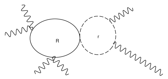
Figure 1: One of the Feynman diagrams of the matrix model.

Simple power counting shows that this graph (and all of the others with these properties) are suppressed by at least nine powers of $R$. The three propagators each give $1/R^{2}$; extracting four velocities gives $1/R^{4}$, and the loop integration gives one power of $R$. Thus the graph goes as $1/R^{9}$. Supersymmetry cancellations might give further suppression, but already this is smaller than $1/R^{7}$. An identical suppression can be found in the background field method used by [10, 9].

One can alternatively do the counting in terms of effective operators. Integrating out first the more massive fields, i.e. integrating over the $R$ loop, yields an effective local operator built of the light fields. Since $x_{1}$ doesn’t couple directly to light fields, this operator must be of the form $(v_{1}-v_{2})^{2}(v_{1}-v_{3})^{2}X^{2}$. Here $X$ represents operators which can couple to the light fields. On dimensional grounds, this should go as $1/R^{9}$. The integral over the light field loop cannot induce compensating powers of $R$.

We can also ask what sorts of terms are generated by the iteration of the one loop matrix model Hamiltonian. It is easy to show that there are no terms of the correct form here as well. We will return to this point in our concluding remarks. One can also easily check that higher loop contributions are further suppressed.

In short, we see that no term of the form

$${(k_{1}\cdot k_{2})(k_{2}\cdot k_{3})(k_{3}\cdot k_{1})\over R^{7}r^{7}}\propto{(v_{1}-v_{2})^{2}(v_{1}-v_{3})^{2}(v_{3}-v_{2})^{2}\over R^{7}r^{7}}$$ (2.3)

can be generated in the matrix model at any loop order.

3 Supergravity

We now turn to the calculation in supergravity. In eleven dimensions, this just means that we need to consider graviton exchange between the external gravitons, so the required vertices can be read off the Einstein lagrangian. The relevant diagrams are shown in Figure 2.

$$\begin{array}[]{ccc}\hskip-142.26378pt\epsfbox[050200200]{SugraGraph1.eps}&\hskip 142.26378pt\epsfbox[050200200]{SugraGraph2.eps}\end{array}$$

Figure 2: The supergravity graphs

To evaluate the graphs, we need to know the structure of the supergravity vertices. These are conveniently collected in [17]. The three graviton vertex appears in eqn. 2.6 of that paper, the four graviton vertex in 2.8. Here we give a brief summary of the computation.

Work in momentum space. Immediately take the limit $q_{2}\approx-q_{3}\gg q_{1}$, where $q_{i}$ are the momentum transfers. The leading terms in the matrix model don’t involve the fermionic variables and thus don’t change the polarizations; helicity-changing terms are suppressed by powers of the impact parameter (or the momentum transfer, in momentum space). So we look for terms in the graviton amplitude

$$k_{1}\cdot k_{3}k_{1}\cdot k_{5}k_{3}\cdot k_{5}\xi_{1}\cdot\xi_{2}\xi_{3}\cdot\xi_{4}\xi_{5}\cdot\xi_{6}\over q_{1}^{2}q_{3}^{2}$$ (3.1)

The vertices where an incoming graviton emits a single, slightly off shell graviton are particularly simple. Calling the incoming and outgoing momenta $k_{1}$ and $k_{2}$, respectively, and $q$ the momentum transfer, and taking the polarization indices to be $\alpha\mu$, $\beta\nu$, $\sigma\gamma$, the only relevant terms (not suppressed by powers of $q$) are

$$P_{3}(k_{1\sigma}k_{2\gamma}\eta_{\mu\nu}\eta_{\alpha\beta})+P_{6}(k_{1\sigma}k_{1\gamma}\eta_{\mu\nu}\eta_{\alpha\beta}).$$

The $P_{i}$’s denote symmetrization in the three gravitons; the subscript denotes the number of distinct permutations. Note that in the limit of interest, the $q$’s are small compared to the transverse momenta, so we need to keep in every instance the smallest possible number of $q$’s. In the first term, then, the only relevant symmetrization is $1\rightarrow 2$, but this gives nothing new; in the second, this does. In this limit, $k_{1}\approx-k_{2}$ (all momenta are defined as flowing into the vertex) so we have simply

$$V_{a}\approx k_{1\sigma}k_{1\gamma}\eta_{\mu\nu}\eta_{\alpha\beta}.$$ (3.2)

Next consider the vertex involving three off shell gravitons. For the kinematic structure of equation (3.1), We are only interested in the term involving $q_{2}\cdot q_{3}\approx-q_{3}^{2}$. There is only one such term:

$$-2P_{3}(q_{1}\cdot q_{3}\eta_{\alpha\nu}\eta_{\beta\sigma}\eta_{\gamma\mu})$$

where the gravitons $1,2,3$ carry indices $\mu\alpha$, $\nu\beta$, $\sigma\gamma$, respectively. The symmetrization produces no additional factors.

Thus for the diagram with the three graviton vertex we obtain

$$(i\kappa^{4})(\xi\cdot\xi)^{3}(k_{1}\cdot k_{3})(k_{1}\cdot k_{5})(k_{5}\cdot k_{3})\left({1\over q_{1}^{2}q_{3}^{2}}\right)$$ (3.3)

The second diagram is the only other relevant one for this structure. We need the four graviton vertex appearing here. For such a vertex, label the incoming lines $k_{1},\mu,\alpha;k_{2}\nu,\beta;q_{3},\sigma,\gamma;q_{4},\rho,\lambda$. Because this diagram already has $1\over q_{3}^{2}q_{1}^{2}$, we can ignore all terms of order $q$ at the vertex. In addition, we must again insure that the helicity on the incoming and outgoing graviton lines is unchanged. A careful examination of the expression for the four graviton vertex indicates that there are only two relevant terms,

$$-P_{12}(k_{1\sigma}k_{2\rho}\eta_{\gamma\lambda}\eta_{\mu\nu}\eta_{\alpha,\beta})-2P_{12}(k_{1,\nu}k_{1,\sigma}\eta_{\beta\gamma}\eta_{\mu\rho}\eta_{\alpha\lambda}).$$

The second term does not obviously preserve helicities. However, if one exchanges $2\rightarrow 4$, then one obtains

$$-P_{12}(k_{1\sigma}k_{2\rho}\eta_{\gamma\lambda}\eta_{\mu\nu}\eta_{\alpha,\beta})-2P_{12}(k_{1,\rho}k_{1,\sigma}\eta_{\lambda\gamma}\eta_{\mu\nu}\eta_{\alpha\beta}).$$

In the first term, exchanging $1\rightarrow 2$ gives an inequivalent result (but exchanging $3\rightarrow 4$ does not). In the second term, exchanging $1$ and $2$ similarly gives an inequivalent result. So at the vertex we have, using $k_{1}=-k_{2}$,

$$-2k_{1,\rho}k_{1,\sigma}\eta_{\lambda\gamma}\eta_{\mu\nu}\eta_{\alpha\beta}.$$

One can now combine this with the three graviton vertices to obtain for the diagrams (note that in this limit, the four-graviton vertex can attach to either of two of the external lines, giving the same result)

$$(-2i\kappa^{4})(\xi\cdot\xi)^{3}(k_{1}\cdot k_{3})(k_{1}\cdot k_{5})(k_{5}\cdot k_{3})\left({1\over q_{1}^{2}q_{3}^{2}}\right)$$ (3.4)

The two contributions do not cancel.

We have done many further checks on these amplitudes. In the next section, we will show that this amplitude agrees with a string computation. It is easy to compute many of the other terms in the vertex and to compare these with a string computation as well, and we have done several additional tests of this sort.

4 Strings

We now turn to the string calculation. We will work in bosonic string theory. The M-point tensor amplitude is given by [18]

$$A_{\mu_{1}\nu_{1}..\mu_{M}\nu_{M}}\zeta_{1}^{\mu_{1}\nu_{1}}..\zeta_{M}^{\mu_{M}\nu_{M}} =\pi\kappa^{M-2}\int d^{2}z_{1}..d^{2}z_{m}{1\over\Delta}$$ (4.1)

$$\prod_{i>j}{(z_{i}-z_{j})^{k_{ij}}}exp\left[\sum_{i>j}{{\zeta_{i}.\zeta_{j}\over(z_{i}-z_{j})^{2}}}-\sum_{i>j}{{k_{i}.\zeta_{j}\over 2(z_{i}-z_{j})}}\right]$$

$$\prod_{i>j}{(\bar{z}_{i}-\bar{z}_{j})^{k_{ij}}}exp\left[\sum_{i>j}{{\bar{\zeta}_{i}.\bar{\zeta}_{j}\over(\bar{z}_{i}-\bar{z_{j})^{2}}}-\sum_{i>j}{{k_{i}.\bar{\zeta}_{j}\over 2(\bar{z}_{i}-\bar{z}_{j})}}}\right]$$

where

$$\Delta={d^{2}Z_{a}d^{2}Z_{b}d^{2}Z_{c}\over|Z_{a}-Z_{b}|^{2}|Z_{a}-Z_{c}|^{2}|Z_{c}-Z_{b}|^{2}}$$ (4.2)

means that three variables are to be given arbitrary values and not integrated. Here we have introduced

$$k_{ij}=k_{i}\cdot k_{j}/4$$ (4.3)

We are interested in terms where the polarizations dot into themselves, thus we need

$$\zeta_{1}.\zeta_{2}\bar{\zeta}_{1}.\bar{\zeta}_{2}\zeta_{3}.\zeta_{4}\bar{\zeta}_{3}.\bar{\zeta}_{4}\zeta_{5}.\zeta_{6}\bar{\zeta}_{5}.\bar{\zeta}_{6}$$ (4.4)

We will in addition choose $z_{6}=\infty,z_{5}=1,z_{4}=0$. This means that all terms involving $z_{6}$ cancel.

The resulting expression has the structure (we will omit the integration symbol henceforth)

$$z_{12}^{k_{12}-2}z_{13}^{k_{13}}z_{14}^{k_{14}}z_{15}^{k_{15}}z_{23}^{k_{23}}z_{24}^{k_{24}}z_{25}^{k_{25}}z_{34}^{k_{34}-2}z_{35}^{k_{35}}$$ (4.5)

multiplied by its complex conjugate .

We are interested in poles involving ${1\over k_{12}}$, ${1\over k_{34}}$, ${1\over k_{56}}$. To isolate singularities of this sort, the following change of variables is helpful:

$$z_{1}=(r_{1}+1)z_{2}~{}~{}~{}~{}~{}z_{2}=z_{2}~{}~{}~{}~{}~{}~{}z_{3}=r_{3}z_{2}$$ (4.6)

The integrand then becomes

$$z_{2}^{-2+k_{56}}r_{1}^{-2+k_{12}}r_{3}^{-2+k_{34}}f(r_{1},r_{3},z_{2})$$ (4.7)

where

$$f(r_{1},r_{3},z_{2})=(1+r_{1}-r_{3})^{k_{13}}(1+r_{1})^{k_{14}}(1-z_{2}-r_{1}z_{2})^{k_{15}}(1-r_{3})^{k_{23}}(1-z_{2})^{k_{25}}(1-r_{3}z_{2})^{k_{35}}$$ (4.8)

In this form, the poles of interest come from the integration regions where the variables go to zero.

Indeed, it is now a simple matter to expand the function $f$ in, say, $r_{1}$,$r_{3}$. Keeping the first order terms isolates the pole $(k_{12}k_{34})^{-1}.$ The remaining $z_{2}$ integral is readily done exactly. The most singular term, proportional to $({k_{12}k_{34}k_{56}})^{-1}$ agrees with the supergravity calculation. The term which interests us, proportional to $k_{13}k_{15}k_{35}(k_{12}k_{34})^{-1}$ is non-vanishing and also agrees with the supergravity result. A more detailed study of this integral shows that the properly normalized amplitude reproduces our supergravity result. Those attempting to verify these statements may find the integral:

$$I(n_{1},n_{2},n_{3},n_{4})=\int d^{2}zz^{A-n_{1}}(1-z)^{B-n_{2}}\bar{z}^{A-n_{3}}(1-\bar{z})^{B-n_{4}}$$

$$=\pi(-1)^{n_{4}}{\Gamma(A+1-n_{1})\Gamma(B+1-n_{2})\Gamma(n_{3}+n_{4}-A-B-1)\Gamma(B+1-n_{4})\over\Gamma(-B)\Gamma(1+B)\Gamma(A+B-n_{1}-n_{2}+2)\Gamma(n_{3}-A)}$$ (4.9)

helpful. As noted earlier, we have also checked many of the other terms in the amplitude against the supergravity computation.

5 Implications

We have not found a satisfactory explanation of the discrepancy we have found. However, there are several potential issues in the calculation.

We must emphasize that we have done a matrix model calculation at a finite value of $N$. This means that we have to compare it to M-theory with a compact lightlike circle as proposed in [2] . One might worry that this brings in complications while evaluating the supergravity amplitude. However, one expects that for a large value of the light-like radius $R$ (or, equivalently, a large value of $N$), the theory on a compact lightlike circle tends to classical 11-dimensional supergravity with corrections that are suppressed as ${1\over R}$. Hence we do not expect corrections from the lightlike compactifications to alter our supergravity result (as the corrections scale differently with $R$ and $N$.) It is possible that this is too naive and that DLCQ M-theory contains terms which are not present in the classical supergravity lagrangian. However, this seems to lead to the counterintuitive conclusion that DLCQ M-theory does not behave as classical supergravity in the low energy limit.

It is also possible that we have blundered in some way in our evaluation of the classical amplitude. This would be the simplest resolution of the puzzle. But we have performed numerous checks of the Feynman rules, as well as of our approach to treating the string computation. The detailed agreement of the two computations is impressive.

Another concern is that the iteration of the one loop matrix model Hamiltonian will generate contributions to the three graviton scattering amplitude. However, these have the wrong $N$ and $R$ dependence to resolve the discrepancy. Indeed, the most singular parts of these graphs are easily seen to reproduce the Feynman diagrams in which a graviton is first exchanged, say, between the first and second line, and then another graviton is exchanged between the second and third.

Let us first review how the $N$ counting goes for the one loop diagram, corresponding to the $2\rightarrow 2$ process. On the matrix model side, the result is proportional to ${N_{1}N_{2}\over R^{3}}(v_{1}-v_{2})^{4}/t$. How does this compare to the supergravity calculation? The invariant amplitude behaves as $\kappa^{2}(k_{1}\cdot k_{2})^{2}/t$. However, this is for relativistically normalized states. To go to non-relativistic normalization, we need to divide by a factor of $\sqrt{k^{+}}$ for each external line. This leaves us with

$$\kappa^{2}k^{+}_{1}k^{+}_{2}(\vec{v}_{1}-\vec{v}_{2})^{4}={N_{1}N_{2}\over R^{3}M_{p}^{9}}(\vec{v}_{1}-\vec{v}_{2})^{4}.$$

This is exactly as above.

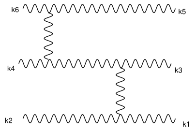
Figure 3: The gravity graph corresponding to the one-loop iteration.

Now let’s consider the Feynman diagrams in the $3\rightarrow 3$ process. First consider the supergravity side. The invariant amplitude is proportional to $(k_{1}\cdot k_{3})^{2}(k_{3}\cdot k_{5})^{2}/k_{3}\cdot q_{3}$, where $q_{3}$ is the small momentum transfer, and we have used the fact that $k_{3}^{2}=0$. In terms of light cone variables, this is

$$(k^{+}_{1}k^{+}_{3})^{2}(v_{1}-v_{2})^{4}(k^{+}_{3}k^{+}_{5})^{2}(v_{2}-v_{3})^{4}\over k_{3}\cdot q_{3}$$

The external state normalization factors give $(k^{+}_{1}k^{+}_{3}k^{+}_{5})^{-1}$. In terms of $N$-dependence, this leaves

$${N_{1}N_{2}^{3}N_{3}(v_{1}-v_{2})^{4}(v_{2}-v_{3})^{4}\over R^{5}k_{3}\cdot q_{3}}$$

It is easy to see how this is reproduced by the matrix model. The iteration of the lowest order Hamiltonian reproduces the velocity factors and gives $N_{1}N_{2}^{2}N_{3}/R^{6}$. The energy denominator is $(\vec{k}_{3}\cdot\vec{q}_{3})/N_{2}R^{-1}$. So we obtain the amplitude above.

One could imagine all sorts of corrections to the matrix model Hamiltonian (at one loop) which would give things like $\vec{q}_{3}\cdot\vec{k}_{3}$ in the numerator, but all contributions will still have the same $N$-dependence. This is not the $N$-dependence of the contribution we want to cancel. (It is also difficult to see how one could obtain the correct $v$-dependence.)

Another possible concern is that with so many legs, it is not straightforward to work in light cone gauge for generic momenta and polarizations. But by studying particular cases one can check that this is not a problem. For example, one can take two of the incoming (and outgoing) polarizations to be the same. In this case, it is easy to see that there are no new contributions with the same dependence on the momenta as those which we have studied here.

It may be that there is a conceptual problem with our understanding of the matrix model. Perhaps there are additional contributions which should be included which can reproduce the missing terms. Such phenomena are familar in light-cone field theory where it is necessary to include contact terms arising from integrating out backward-moving particles. In previous calculations, such terms have been suppressed by powers of $N$. However, in the present case, they potentially have the correct $N$ dependence to generate the missing term. We have not been able to understand in any detail how this might work; if it is the resolution, the question will be whether there is some simple rule to generate these extra terms in the framework of the matrix model. We should note that the arguments of [14] strongly suggest that this cannot be the source of the difficulty. It may also be that the use of the effective Hamiltonian is problematic. For example, the effective action presumably contains acceleration terms, which may complicate the Hamiltonian treatment. Finally, there is of course the possibility that the finite $N$ matrix model, as presently formulated, does not reproduce DLCQ M-theory.

One might wonder if the derivation by Dijgraff, Verlinde and Verlinde [13] of the three string vertex already implies that all graviton scattering amplitudes must be reproduced correctly in the matrix model. This is not straightforward. Light cone string theory contains an infinite set of additional terms (the so-called contact terms) that are not derived from the string vertex, but instead must be put in by hand to restore Lorentz invariance . One such term is the famous $v^{4}/r^{7}$ term that we have already referred to. The term of interest in this paper is another such term. The question is then whether some property such as analyticity of the amplitude implies that the contact terms must be reproduced correctly if the string vertices are reproduced (along the lines of [19].) We do not know the answer to this question. One must also note that higher order corrections to the three-string vertex which were undetermined in [13] may be important.

The most impressive and concise argument to date for the validity of the matrix model is that of [14]. We do not currently understand how this argument might be reconciled with the apparent discrepancy we have found.

There is also an issue as to whether the discrepancy we have found disappears in the infinite momentum limit. This can happen because the size of the zero-brane clusters forming a graviton grows with $N$. In the limit as $N$ tends to infinity, the clusters are infinitely large, and there is no sense in which the separation between the clusters can be assumed to be large. This in turn means that we cannot find the effective action by integrating out massive strings as we have done here. To do the calculation in this limit, one needs more knowledge of the bound state wave function. It is hence conceivable that the discrepancy vanishes in the infinite momentum limit.

Note added: After the completion of this work, we received a paper by M. Douglas and H. Ooguri [21], which describes a discrepancy between the matrix model and supergravity in the presence of curved backgrounds, following the analysis of [20]. It seems likely that this discrepancy is related to the one described in this work.

6 Acknowledgments

We thank W. Fischler, J. Polchinski, N. Seiberg, E. Silverstein, S. Shenker, and L. Susskind for extensive discussions. S. Shenker, in particular, has suggested for some time that multigraviton scattering would provide an interesting test of the matrix model, and W. Fischler collaborated at an early stage. The work of M.D. was supported in part by the Department of Energy, and in part by the Stanford Institute for Theoretical Physics. The work of A.R. was supported in part by the Department of Energy under contract no. DE-AC03-76SF00515.

References

- [1] T. Banks, W. Fischler, S. Shenker and L. Susskind, Phys. Rev. D55 (1997) 5112; hep-th/9610043.
- [2] L. Susskind, hep-th/9704080.
- [3] L. Susskind, hep-th/9611164.
-
[4]
W. Taylor IV, Phys. Lett.
B394 (2997) 283; hep-th/9611042;
O.J. Ganor, S. Ramgoolam and W. Taylor IV, Nucl. Phys. B492 (1997) 191; hep-th/9611202. - [5] W. Fischler, E. Halyo, A. Rajaraman and L. Susskind, hep-th/9703102.
- [6] M.Rozali, hep-th/9702136.
- [7] M. Berkooz, M. Rozali and N. Seiberg, hep-th/9704089.
- [8] N. Seiberg, hep-th/9705221.
- [9] K. Becker, M. Becker, J. Polchinski and A. Tseytlin, Phys.Rev. D56 (1997) 3174; hep-th/9706072.
-
[10]
G. Lifschytz, hep-th/9612223.
O. Aharony and M. Berkooz, hep-th/9611215.
G. Lifschytz and S. Mathur, hep-th/9612087. -
[11]
I. Chepelev and A. A. Tseytlin, hep-th/9709087.
E. Keski-Vakkuri and P. Kraus, hep-th/9709122. -
[12]
J. Polchinski and P. Pouliot, NSF-ITP97-27, hep-th/9704029.
C.Fraser and D. Tong, hep-th/9710098. - [13] R. Dijkgraaf, E. Verlinde and H. Verlinde, Nucl. Phys. B500 (1997) 43; hep-th/9703030.
- [14] N. Seiberg, hep-th/9710009.
- [15] M. Douglas, D. Kabat, P. Pouliot and S. Shenker, Nuc. Phys. B 485 (1997) 85; hep-th/9608024.
- [16] C. Bachas, Phys. Lett. B 374 (1996) 37; hep-th/9511043.
- [17] S. Sannan, Phys. Rev. D34 (1986) 749.
- [18] H. Kawai, D.C. Lewellyn and S.H.H. Tye, Nuc. Phys. B 269 (1986) 1 .
- [19] M. Green and N. Seiberg, Nuc. Phys. B 299 (1988) 559 .
- [20] M. Douglas, H. Ooguri and S. Shenker, Phys. Lett. B 402 (1997) 36; hep-th/9702203.
- [21] M. Douglas and H. Ooguri, hep-th/9710178.