Polchinski equation, reparameterization invariance and the derivative expansion

The connection between the anomalous dimension and some invariance properties of the fixed point actions within exact RG is explored. As an application, Polchinski equation at next-to-leading order in the derivative expansion is studied. For the Wilson fixed point of the one-component scalar theory in three dimensions we obtain the critical exponents $\eta=0.042$, $\nu=0.622$ and $\omega=0.754$.

UB-ECM-PF 97/05

1 Introduction

The derivative expansion [1] is, up to now, the most reliable approximation available when dealing with exact renormalization group equations (exact RG equations, hereafter). Nevertheless, although quite simple at lowest order, some subtleties appear beyond it.

They are mostly related to the preservation of the so-called reparameterization invariance [3, 4] through the derivative expansion. In bold terms the problem is the following. It is known that an overall normalization of the action does not matter and, therefore, one may define RG transformations in such a way that its fixed points (FPs) are normalized to any pre-specified value. However, does this freedom survive order by order in the derivative expansion? And if not, which is the “best” normalization, in the sense that the expansion converges the most rapidly (if at all)?

The problem is not merely academic because, as we will see, invariance of universal quantities under reparameterizations is the ultimate responsible of the uniqueness of the anomalous dimension $\eta$, much in the same way as the invariance under rescalings in a linear system over-determines its solution, effectively quantizing its eigenvalues.

These two questions have been successfully answered for equations regarding the “quantum effective action” [1]. Essentially, one chooses RG transformations in such a way that some invariance properties of the full equation are maintained order by order in the derivative expansion (see below for details). In contrast, for the Polchinski equation [5], these points seem not even been addressed.

Specifically, in Ref. [6] a calculation of critical exponents for one-component scalar theories was presented, using Polchinski equation up to second order in the derivative expansion. An arbitrary normalization of the action was chosen, and a large class of transformations analyzed. Critical indices were found to be, not surprisingly, transformation-dependent, as the arbitrary truncation of the expansion introduces spurious dependencies. These kind of ambiguities were partially solved by the usual criterion of minimal sensitivity [7], thus choosing the transformation which one hopes to converge most rapidly when derivative expanded.

Two problems remain, nevertheless, open. On one hand, as we have already mentioned, the possibility of non-standard normalizations was not addressed, nor a kind of reparameterization invariance sought. On the other hand, a one-parameter family of transformations was left over for which, apparently, a minimal sensitivity criterion cannot be found. Different transformations within this line give slightly different RG eigenvalues although around a FP with significantly different anomalous dimensions. Thus one is left with the impression that clear results cannot be obtained and that the derivative expansion as it stands is thus of limited use beyond the leading order, at least for those type of equations.

The first problem is specially annoying, because, although we expect that different transformations have different convergence properties and, thus, give different results, we do not expect that the same RG transformations may give a non-unique answer.

The article is organized as follows. We first review in Section 2 the derivation of Polchinski equation together with its projection. The leading order of the derivative expansion is reviewed in Section 3. In Section 4 we explain the connection of the anomalous dimension $\eta$ with the reparameterization symmetry and its relevance for next-to-leading order computations. A (failed) search for RG transformations invariant under a linear representation of the symmetry group is discussed in Section 5. Finally, in Section 6, a detailed description of our method of calculation, together with the obtained results for critical indices $\eta$, $\nu$ (given by the inverse of the relevant RG eigenvalue) and $\omega$ (minus the first irrelevant RG eigenvalue) of the Ising universality class in three dimensions, is reported. Two peripheral subjects are left for the Appendices.

2 Equation

Exact RG equations express the change of some quantity (usually the classical action) under an infinitesimal RG transformation. Polchinski equation deals with one-component bosonic models regulated as

$$S[\phi]=\frac{1}{2}\int_{p}p^{2}K^{-1}(p^{2})\phi_{-p}\phi_{p}+S_{I}[\phi],$$ (1)

with some function $K(p^{2})$ decreasing faster than any polynomial for large $p^{2}$. Conventions are as follows. We work on Euclidean momentum space of dimension $d$, with $\phi_{p}$ being the $p$ mode of the Fourier transformed field and $\int_{p}\equiv\int\frac{d^{d}p}{(4\pi)^{d}}$. All variables are dimensionless. Thus in dimensionful units the regulating function should be $K(p^{2}/\Lambda^{2})$, $\Lambda\equiv\Lambda_{0}e^{-t}$ with $\Lambda_{0}$ some fixed scale and $t$ the label that parameterize the RG flow.

RG transformations are usually defined in two steps, first some blocking—thinning of degrees of freedom—and afterwards a rescaling of variables so that FPs are possible. The first step is accomplished by splitting the field into

$$\phi_{p}=\phi^{(0)}_{p}+\phi^{(1)}_{p},$$ (2)

with the field $\phi^{(0)}_{p}$ propagated by

$$\frac{K(p^{2}e^{2\tau})}{p^{2}}$$ (3)

and $\phi^{(1)}_{p}$ by

$$\frac{K(p^{2})-K(p^{2}e^{2\tau})}{p^{2}}=-2\tau K^{\prime}(p^{2})+{\cal O}(\tau^{2}).$$ (4)

The field $\phi^{(1)}_{p}$ is then to be integrated out, thus effectively eliminating modes mainly within the shell $e^{-\tau}\!<|p|\leq 1$. For infinitesimal $\tau$ the result is that functional integration over the full field $\phi_{p}$ is equivalent to integration over $\phi^{(0)}_{p}$ with the action

$$\frac{1}{2}\int_{p}p^{2}K^{-1}(p^{2}e^{2\tau})\phi^{(0)}_{p}\phi^{(0)}_{-p}+S_{I}+\tau\left\{\int_{p}S^{\prime}_{I;-p}K^{\prime}(p^{2})S^{\prime}_{I;p}-\int_{p}K^{\prime}(p^{2})S^{\prime\prime}_{I;-p,p}\right\},$$ (5)

with

$$S_{I}\equiv S_{I}[\phi^{(0)}],\qquad S^{\prime}_{I;p}\equiv\frac{\delta S_{I}}{\delta\phi_{p}}[\phi^{(0)}],\qquad S^{\prime\prime}_{I;-p,p}\equiv\frac{\delta S_{I}}{\delta\phi_{-p}\delta\phi_{p}}[\phi^{(0)}].$$ (6)

See Ref. [8] for further details.

Rescaling of variables is carried out with

$$p\equiv\tilde{p}e^{-\tau},\ \ \ \phi_{p}^{(0)}\equiv\phi_{\tilde{p}}e^{\tau\frac{d+2-\eta}{2}},$$ (7)

where $\eta$ is some $t$-dependent parameter which coincides with the field anomalous dimension in the vicinity of a FP.

Finally, renaming $\tilde{p}\rightarrow p$,

$$\dot{S}[\phi] \equiv \lim_{\tau\longrightarrow 0}\frac{S(t+\tau)-S(t)}{\tau}$$ (8)

$$= \int_{p}S^{\prime}_{-p}K^{\prime}(p^{2})S^{\prime}_{p}-\int_{p}K^{\prime}(p^{2})S^{\prime\prime}_{-p,p}-2\int_{p}p^{2}K^{-1}(p^{2})K^{\prime}(p^{2})\phi_{p}S^{\prime}_{I;p}$$

$$\mbox{}+dS-\frac{d-2+\eta}{2}\int_{p}\phi_{p}S^{\prime}_{p}-\int_{p}\phi_{p}\,p\!\cdot\!\frac{\partial^{\prime}}{\partial p}\,S^{\prime}_{p},$$

where we have (partially) returned back to the full action and written a prime in the last term to mean that it serves only to count momenta, thus delta functions of momentum conservation should not be derived.

The derivative expansion amounts to consider a subset of interactions, with a maximum power of momenta in their coefficients, and to consider the RG Eq. (8) for these terms as if they form a closed subset under the RG, that is, to approximate their evolution as if any other operators out of the subset do not contribute.

We deal with the expansion up to two derivatives, with an action

$$S[\phi]=V[\phi_{0}]\int d^{d}x+Z[\phi_{0}]\,\frac{1}{2}\int_{p}p^{2}K^{-1}(p^{2})\phi_{-p}\phi_{p},$$ (9)

which produces two coupled partial differential equations,

$$\dot{f} = 2K^{\prime}(0)ff^{\prime}-({\textstyle\int}K^{\prime})f^{\prime\prime}-({\textstyle\int}p^{2}K^{\prime})Z^{\prime}+\frac{d+2-\eta}{2}\,f-\frac{d-2+\eta}{2}\,\varphi f^{\prime},$$

$$\dot{Z} = 2K^{\prime}(0)fZ^{\prime}+4K^{\prime}(0)f^{\prime}Z+2K^{\prime\prime}(0)f^{\prime 2}-({\textstyle\int}K^{\prime})Z^{\prime\prime}-4K^{-1}(0)K^{\prime}(0)f^{\prime}$$ (10)

$$\mbox{}-\eta Z-\frac{d-2+\eta}{2}\,\varphi Z^{\prime},$$

with $\varphi\equiv\phi_{0}$ and $f(\varphi)\equiv V^{\prime}(\varphi)$. For convenience, we work with such equations after the rescalings

$$\varphi\longrightarrow\sqrt{-{\textstyle\int}K^{\prime}}\,\varphi,\ \ \ f\longrightarrow\frac{\sqrt{-{\textstyle\int}K^{\prime}}}{-K^{\prime}(0)}\,f,\ \ \ Z\longrightarrow K^{-1}(0)Z;$$ (11)

so that,

$$\dot{f} = -2ff^{\prime}+f^{\prime\prime}+AZ^{\prime}+\frac{d+2-\eta}{2}\,f-\frac{d-2+\eta}{2}\,\varphi f^{\prime},$$ (12)

$$\dot{Z} = -2fZ^{\prime}-4f^{\prime}Z+2Bf^{\prime 2}+Z^{\prime\prime}+4f^{\prime}-\eta Z-\frac{d-2+\eta}{2}\,\varphi Z^{\prime},$$

where the transformation dependencies are bound to the parameters

$$A\equiv\frac{(-K^{\prime}(0))(-{\textstyle\int}p^{2}K^{\prime})}{(-{\textstyle\int}K^{\prime})K(0)},\ \ \ B\equiv\frac{K^{\prime\prime}(0)K(0)}{(-K^{\prime}(0))^{2}}.$$ (13)

These conventions coincide with those of Ref. [6], except for the arbitrariness of $K(0)$.

Eigenvalues of the RG control deviations from the FP. They can be calculated from the linearized version of the RG transformations. That is, by taking $f(\varphi,t)=f_{FP}(\varphi)+re^{\lambda t}g(\varphi)$, $Z(\varphi,t)=Z_{FP}(\varphi)+re^{\lambda t}h(\varphi)$, with $f_{FP}(\varphi)$ and $Z_{FP}(\varphi)$ the FP values and $r\ll 1$ a coupling constant,

$$\lambda g = -2gf^{\prime}_{FP}-2f_{FP}g^{\prime}+g^{\prime\prime}+Ah^{\prime}+\frac{d+2-\eta}{2}g-\frac{d-2+\eta}{2}\varphi g^{\prime},$$

$$\lambda h = 4Bf^{\prime}_{FP}g^{\prime}-4hf^{\prime}_{FP}-4Z_{FP}g^{\prime}-2h^{\prime}f_{FP}-2Z^{\prime}_{FP}g+h^{\prime\prime}+4g^{\prime}$$

$$-\eta h-\frac{d-2+\eta}{2}\varphi h^{\prime},$$

with $\lambda$ being the eigenvalue.

3 Local potential approximation

In this section we concisely discuss the results obtained within the first order of the derivative expansion—the so-called local potential approximation (LPA, hereafter).

That is, we truncate the action simply to

$$S=\frac{1}{2}\int_{p}p^{2}K^{-1}(p^{2})\phi_{-p}\phi_{p}+V(\phi_{0})\int d^{d}x.$$ (15)

The requirement that the non-potential term of Eq. (15) remains fixed under the RG forces $\eta=0$, while the evolution of $V(\varphi)$ is (cf. Eq. (12))

$$\dot{f}=-2ff^{\prime}+f^{\prime\prime}+AZ^{\prime}+\frac{d+2}{2}\,f-\frac{d-2}{2}\,\varphi f^{\prime}.$$ (16)

The FPs appear as the $\dot{f}=0$ solutions of Eq. (16),

$$0=-2ff^{\prime}+f^{\prime\prime}+AZ^{\prime}+\frac{d+2}{2}\,f-\frac{d-2}{2}\,\varphi f^{\prime}.$$ (17)

Since this is a second order differential equation one may expect, in principle, a two-parameter set of FPs. This is not true, of course. First of all, $Z_{2}$ symmetry imposes $f(0)=0$, thus reducing the arbitrariness to a uniparametric family of FPs (labeled by, for instance, $\gamma\equiv f^{\prime}(0)$). Nevertheless, all but a finite number of $\gamma$’s correspond to solutions which end with a singularity at a finite $\varphi=\varphi_{0}$,

$$f(\varphi)\sim\frac{1}{\varphi_{0}-\varphi}\qquad\hbox{as $\varphi\to\varphi_{0}$}.$$ (18)

Therefore, if we want $f(\varphi)$ to be defined for the whole range $0\leq\varphi<\infty$, the possible FPs reduce to a finite set.

The Gaussian FP corresponds to

$$f(\varphi)=0.$$ (19)

It is easy to compute its eigenvalues because, after the rescaling $\varphi=2\tilde{\varphi}/\sqrt{d-2}$, the eigenvalue equation,

$$g^{\prime\prime}(\tilde{\varphi})-2\tilde{\varphi}g^{\prime}(\tilde{\varphi})+2\frac{d+2-2\lambda}{d-2}g(\tilde{\varphi})=0,$$ (20)

is known to have polynomially bounded solutions, odd in $\tilde{\varphi}$ (we want to maintain $Z_{2}$ symmetry), only for

$$\lambda=d-n(d-2),\qquad n=1,2,\ldots$$ (21)

In this case the solutions are the well-known Hermite polynomials of odd degree [2]. The case $n=0$, $g(\varphi)=0$ corresponds to the identity operator (see Appendix A). It is curious that this very same eigenvectors appear also within the LPA of other RG equations, although the aspect of the exact result may be quite different [9, 2]. Being the FP action not a universal quantity, this behavior should be probably regarded just as a coincidence.

One can also identify analytically a FP which must correspond to the non-critical high temperature FP,

$$f(\varphi)=\varphi.$$ (22)

Its eigenvectors are also Hermite polynomials but without relevant directions,

$$\lambda=d-n(d+2),\qquad n=1,2,\ldots$$ (23)

The case $n=0$ corresponds again to the identity operator. Because of the simplicity of the approximation, one can also explicitly write down the renormalized trajectory between the Gaussian FP and this one here,

$$f(\varphi,t)=re^{2t}\varphi/(1+re^{2t}),$$ (24)

with $r$ being some (fixed) coupling constant [2].

This latter FP is of no physical interest, but we wanted to quote it mainly because it has to be taken into account in the numerical work to follow, in order not to confuse it with the Wilson FP.

Finally, there is also the FP corresponding to the Ising universality class, known as Wilson FP. Unfortunately, one cannot obtain it analytically and must rely on numerical methods.

The idea is to integrate Eq. (17) from initial conditions $f(0)=0$ and $f^{\prime}(0)=\gamma$, and scan over different $\gamma$’s until the correct asymptotic behavior is reached,

$$f(\varphi)\sim\varphi+C\varphi^{\frac{d-2}{d+2}}+\cdots\quad\hbox{as $\varphi\to\infty$,}$$ (25)

with $C$ being some arbitrary constant (which one must find out). Note that, as explained above, $C=0$ coincides with an uninteresting FP which should be discarded. For details about the numerical method we refer the interested reader to Appendix B.

The eigenvectors are obtained in a similar manner. The linearized RG equation at this order is simply

$$\lambda g=-2gf^{\prime}_{FP}-2f_{FP}g^{\prime}+g^{\prime\prime}+\frac{d+2}{2}g-\frac{d-2}{2}\varphi g^{\prime}.$$ (26)

In general its solutions will grow exponentially,

$$g(\varphi)\sim e^{\varphi^{2}}+\cdots\quad\hbox{as $\varphi\to\infty$,}$$ (27)

whereas for a countable set of $\lambda$’s it will be much smoother,

$$g(\varphi)\sim\varphi^{\frac{d-2-2\lambda}{d+2}}+\cdots\quad\hbox{as $\varphi\to\infty$.}$$ (28)

Choosing the latter behavior, we obtain, from the first two eigenvalues, $\nu=0.649\,6$ and $\omega=0.655\,7$ in $d=3$. See Refs. [6, 2].

Finally, we should mention that with our approach of focusing on $f(\varphi)\equiv V^{\prime}(\varphi)$ instead of directly on $V(\varphi)$ we are always missing the identity operator. A discussion about it is postponed to Appendix A.

4 The anomalous dimension $\eta$

In this section we explore the connection between the anomalous dimension $\eta$ and some exact symmetries of the FP action.

There is a large class of RG transformations which are denoted as linear, because the blocked variables are linearly related to the old ones [10]. It includes the transformations expressed as exact differential equations. One of their main features is that they present always arbitrary parameters, usually in their rescaling part.

These parameters are to be fine-tuned in order to obtain a FP. For instance, the Gaussian FP of Polchinski equation,

$$\frac{1}{2}\int_{p}p^{2}K^{-1}(p^{2})\phi_{-p}\phi_{p},$$ (29)

appears solely after the choice $\eta=0$. If $\eta$ is set to some other value (in $d=4$), either no FP is obtained, or only a non-interacting, infinitely massive FP comes out, with no interest for Physics.

A comment is in order. The operator $\phi_{0}$ happens to be the first magnetic eigenvector, with eigenvalue $\lambda_{M}=(d+2-\eta)/2$. And, from the known scaling relation,

$$\hbox{(anomalous dimension)}=d+2-2\lambda_{M}=\eta=0.$$ (30)

Thus the free parameter $\eta$ is directly the anomalous dimension. This is a general scenario, although the precise relation between the anomalous dimension and the free parameters is not always that simple [12, 3]. The key point, nonetheless, is that there always exists some parameters in the transformations themselves which need to be fine-tuned in order to reach a FP, and that these parameters are closely related to the field anomalous dimension at the FP.

On the other hand, any FP is usually associated with a whole family of them, with different actions but with the same critical properties. For instance, in the Gaussian case above, one finds the line of FPs,

$$\frac{1}{2}\int_{p}p^{2}K^{-1}(p^{2})\left[1+aK(p^{2})\right]^{-1}\phi_{-p}\phi_{p},$$ (31)

where $a$ is some (real) parameter with $aK(p^{2})>-1$ for any $p$.

Of course, this is not a surprise, since it is precisely this arbitrariness what makes the set of FP solutions finite. It is like the scale invariance of a linear eigenvalue problem. The latter may have apparently a solution for each arbitrary eigenvalue, but the fact that we can choose the normalization of the eigenvector at will over-determines the system, making that only a discrete set of eigenvalues are allowed. The fine-tuning procedure, thus, is due to some sort of underlying arbitrariness (some sort of symmetry). Had a FP equation no invariances at all, no parameter would have to be fine-tuned.

The form of the eigenperturbations about the FP also vary along the line of FP. For instance, the mass term is

$$\frac{1}{2}\int_{p}[1+aK(p^{2})]^{-2}\phi_{-p}\phi_{p},$$ (32)

with eigenvalue 2.

Therefore, to summarize, linear RG transformations present two important features: They contain free parameters which have to be fine-tuned in order a FP to be reached; this feature reflects an underlying symmetry which manifest itself in a line of equivalent FPs.

So far for exact computations. Let us now discuss the actual case, that is, let us discuss how this picture survives under the (up to now) unavoidable approximations of RG equations. For definiteness, we take the derivative expansion at second order, Eq. (12), but the following should be easily extendible to any feasible truncation.

First of all, it is clear that the line of FPs, Eq. (31), is hard to reproduce well: Each FP has different ${\cal O}(p^{4})$ terms and higher and only those with such terms comparatively small will be correctly described by our truncation. Therefore, one immediate consequence is that it is not that harmless to blindly choose one normalization (one value of $a$) of our FP action when some truncation is involved; e.g., in the Gaussian FP above, several choices of the parameter $a$ will be quite faithful while others will probably poorly capture the properties of the FP.

Moreover, the opposite phenomenon also takes place: One also finds truncated FPs for the wrong choice of the transformation parameter $\eta$. To understand better this annoying feature, let us recall Wegner-Houghton equation [13, 2],

$$\dot{S} = \lim_{\tau\rightarrow 0}\frac{1}{2\tau}\int_{e^{-\tau}<|p|\leq 1}\left[\ln S^{\prime\prime}_{-p,p}-S^{\prime}_{-p}S^{\prime}_{p}(S^{\prime\prime}_{-p,p})^{-1}\right]_{\begin{array}[]{l}\scriptstyle\phi_{p}=0\\ \raise 3.01389pt\hbox{$\scriptscriptstyle e^{-\tau}<|p|\leq 1$}\end{array}}$$ (36)

$$\mbox{}+dS-\frac{d-2+\eta}{2}\int_{p}\phi_{p}S^{\prime}_{p}-\int_{p}\phi_{p}\,p\!\cdot\!\frac{\partial^{\prime}}{\partial p}\,S^{\prime}_{p}.$$

A line of FPs is obtained here with

$$\int_{|p|\leq 1}\frac{d^{d}p}{(2\pi)^{d}}p^{2-\epsilon}\phi_{-p}\phi_{p}$$ (37)

and $\eta=\epsilon$. This phenomenon is of quite different nature as the similar one described above. There the whole line shares the same critical properties, here it does not; there we have well-behaved actions throughout the fixed line, here nearly all of them are terribly non-local (in the sense that we cannot expand the action integrand in a power series of $p^{2}$). What happens is that we have one physical FP (the $\epsilon=0$ case) and a line of spurious ones.

For exact calculations this is not a problem since RG transformations always map local actions into local actions and thus only the $\epsilon=0$ FP may be reached. Nevertheless, simply studying $V(\varphi)$ and $Z(\varphi)$, one may not be able to distinguish non-local FPs from the local, physically meaningful, one.

The recipe to cope these problems is not evident. We have, nevertheless, some hints. Clearly, one should succeed if one manages to compute a FP as local as possible (ideally, one FP with only the $V(\varphi)$ and $Z(\varphi)$ terms). The problem is to try to reach this goal without computing the next order of ones expansion. The key is to try to check, within the given order, some known property of the exact solution, and take the approximate FP which best reproduces it.

A glance at linear systems again may help. Let us imagine that in an eigenvalue problem of linear algebra, one is so bold to approximate it in such a way that eigenvalues are no longer invariant under re-normalizations of the corresponding eigenvectors. One would probably find no quantization of eigenvalues. However, if one insists, after all, to make sense of the approximation, a clever choice would be to look for the eigenvalues which are, to some extent, invariant under rescalings of their eigenvectors. This is, in fact, the method used from time to time for exact RG equations, following the procedure of Ref. [3, 4].

The trick is to find the FP which is first-order (at least) independent of the free parameters. This feature results in the presence of a redundant operator [14] which is marginal or nearly marginal. It has to be redundant because it may not generate true RG trajectories, but simply reparameterizations of the theory; it has to be nearly marginal because it generates, at least approximately, a line of equivalent FPs (the equivalence being guaranteed by the redundancy).

In our computations, therefore, we first plot the anomalous dimension versus the normalization of the kinetic term. It is seen that this curve presents always a maximum, which we regard as the best approximation for the actual anomalous dimension. This is further checked by the finding of a nearly marginal operator, which is known not to exist in the physical spectrum. See Section 6 for the details.

Before ending, let us make one further remark. The criterion explained so far relies on an invariance property of the physical, local, action. This does not mean that non-local FPs do not present their own set of symmetries under reparameterizations. But the claim is that the properties of local solutions should be well-described by local approximations. On the contrary, the analogous of the redundant marginal operator found for local FPs should be terribly non-local and, thus, poorly mapped within the truncation. So poorly that they do not even show up [3].

5 Linearly symmetric RG transformations

Before going on to actual computations, we would like to address one more issue. One knows that the accurate anomalous dimension $\eta$ should be close to the one for which the action presents an (approximate) reparameterization symmetry. That is, why do we not choose RG transformations for which the symmetry is linearly realized, and try to keep this realization through the derivative expansion? This is, in fact, the approach taken in Ref. [1] for the effective-action type of exact RG equations.

The search for such class of transformations is reported in this section. The conclusions turn out to be, unfortunately, rather deceptive. We find a class of regulators with a linearly realized reparameterization symmetry for the exact equations; but, first, the symmetry is broken at finite order in the derivative expansion; and, second, the regulators associated with such transformations turn out not to regulate, at least not in a finite order in the derivative expansion. Therefore, one is lead to the general scenario outlined in the previous section: One must scan a range of normalizations and decide on some kind of locality criteria which is the most reliable one.

Let us seek some functions ${\cal K}(\tilde{p}^{2})$ and ${\cal F}(\tilde{p}^{2})$ such that the transformations

$$p=\lambda\tilde{p},\qquad K(\lambda^{2}\tilde{p}^{2})={\cal K}(\tilde{p}^{2}),\qquad\phi_{\lambda\tilde{p}}={\cal F}(\tilde{p}^{2})\tilde{\phi}_{\tilde{p}}$$ (38)

on an action converts it into another action that satisfies the same RG equation.

In order to obtain an action that satisfies again a Polchinski-kind equation, these functions must satisfy

$${\cal K}^{-1}{\cal K}^{\prime}-{\cal F}^{-1}{\cal F}^{\prime} = K^{-1}K^{\prime}$$

$$\lambda^{-d-2}{\cal F}^{-2}{\cal K}^{\prime} = K^{\prime},$$ (39)

with solutions

$${\cal K}(p^{2})=\frac{\lambda^{\kappa}K(p^{2})}{1+a(\lambda)K(p^{2})},\qquad{\cal F}(p^{2})=\frac{\lambda^{\frac{\kappa-d-2}{2}}}{1+a(\lambda)K(p^{2})},$$ (40)

for some function $a(\lambda)$ and a real number $\kappa$.

If we further require the RG transformations to be exactly the same as those of the initial action, the regulator must satisfy

$$K(\lambda^{2}p^{2})=\frac{\lambda^{\kappa}K(p^{2})}{1+a(\lambda)K(p^{2})},$$ (41)

which implies

$$K(p^{2})=\frac{\kappa/\alpha}{1+\left(p^{2}/q^{2}\right)^{\kappa/2}},$$ (42)

with $\alpha\equiv-a^{\prime}(1)$ and $q^{2}$, $\kappa$ real non-negative numbers. This are the regulators previously reported in Ref. [15].

If we were to use the above regulators, then, for every FP, there would exist a whole line of them, corresponding to different parameterizations of the action (different choices of the dummy variables $\phi$ and $p$). The FPs within the line would be related by simple linear transformations, generated by a marginal redundant operator, as corresponds to any reparameterization. All the FPs would be physically equivalent as long as infra-red properties are concerned [14, 3]. And if these RG transformations were used, then the discussion on normalizations would be totally void. Unfortunately, as we have pointed out above, there are important objections.

First, this kind of symmetry does not in general hold order by order in the derivative expansion, unless $a(\lambda)\equiv 0$, as can be easily stated by considering Eq. (2).

Second, the above class of functions $K(p^{2})$ do not regulate, at least they do not when we consider a fixed order in the derivative expansion, because they behave asymptotically as polynomials. That is, a simple study of one-loop diagrams (see Fig. 1) show, for instance, that the second term of the RG Eq. (8) is not finite at ${\cal O}(p^{2n})$ in the derivative expansion with regulators of Eq. (42) whenever $n\geq\kappa+1-d/2$.

Figure 1: Feynman diagram representing the second term in Polchinski equation. The shadow area stands for a generic vertex (which contributes with a coefficient of ${\cal O}(p^{2n})$ at $n$-th order in the derivative expansion and the thick solid line stands for a propagator $\propto K^{\prime}(p^{2})$. As usual one has to integrate over the closed loop.

The conclusion is, therefore, that the symmetry cannot be linearly implemented order by order in the derivative expansion, in contrast to other equations [1] for which the maintenance of reparameterization invariance selects a preferred scheme. Polchinski equation in this sense is unfortunate: One cannot avoid scanning over different normalizations and selecting a criterion to discriminate among them. The true FP corresponds only to one of the possible normalizations; the rest should probably describe non-local actions.

Finally, let us look again at the Gaussian FP, Eq. (31). It can be found with a regulator of the form of Eq. (42), and in such a case we have a nice example of the symmetry we have talked about. Our second objection does not apply here, since the Gaussian FP is ultra-violet finite anyhow. Nonetheless, the example shows that linear transformations are not the whole story, since, even for arbitrary choices of the regulating function $K(p^{2})$, the line of FPs exist and it has to be generated by non-linear transformations. This last possibility is what we are seeking for the Wilson FP in $d=3$.

6 Results

6.1 Gaussian FP

We have already solved the FP equation within the Gaussian FP exactly, and also for the LPA. Let us briefly review how it appears in second order in the derivative expansion.

It consists solely on a kinetic term with a constant potential, that is,

$$f(\varphi)=0,\qquad Z(\varphi)=\frac{1}{1+aK(0)}.$$ (43)

And, from the second equation in (12), $\eta=0$.

The eigenvectors have a quite simple expression in the case $a=0$. Namely, there appear the same Hermite polynomials for $g(\varphi)$, with $h(\varphi)=0$, obtained when dealing with the LPA, with eigenvalues $\lambda=d-n(d-2)$.

There are also other eigenvectors with (for $a=0$) $g(\varphi)=0$ and the function $h(\varphi)$ a solution of

$$h^{\prime\prime}(\tilde{\varphi})-2\tilde{\varphi}h^{\prime}(\tilde{\varphi})-2\frac{2\lambda}{d-2}h(\tilde{\varphi})=0,$$ (44)

with $\tilde{\varphi}\equiv\frac{\sqrt{d-2}}{2}\varphi$. Again they are Hermite polynomials, this time of even degree, and their eigenvalues

$$\lambda=-n(d-2),\qquad n=0,1,\ldots$$ (45)

The general form for these last perturbations of the FP action is, for the $n$-th such operator,

$$\frac{1}{2}\int dx\,(\partial\phi)^{2}\phi^{2n}(x)+\cdots,$$ (46)

with the dots standing for terms with less number of fields. All of them are irrelevant but the one with $n=0$, which is a marginal redundant operator, $\frac{1}{2}\int dx(\partial\phi)^{2}$, that generates a line of equivalent FPs. It clearly corresponds to a change of normalization of the original FP action.

The general case $a\neq 0$ is technically a bit more complicated. The eigenvalue equations are now

$$\lambda g = g^{\prime\prime}+Ah^{\prime}+\frac{d+2}{2}g-\frac{d-2}{2}\varphi g^{\prime},$$ (47)

$$\lambda h = \frac{aK(0)}{1+aK(0)}g^{\prime}+h^{\prime\prime}-\frac{d-2}{2}\varphi h^{\prime}.$$

The marginal redundant operator is still $g(\varphi)=0$, $h(\varphi)=\mbox{constant}$, of course. And the mass operator also conserves its form, $g(\varphi)=\varphi$, $h(\varphi)=0$, but it is clear that the tower of eigenvectors of the form of Hermite polynomials will not survive and a more complicate computation has to be done. For instance, the eigenvector with eigenvalue $\lambda=4-d$ (the “$\int d^{d}x\,\phi^{4}(x)$” operator) is, for $d\neq 4$,

$$g(\tilde{\varphi}) = 8\tilde{\varphi}^{3}-\left(12+6A\frac{aK(0)}{1+aK(0)}\right)\tilde{\varphi},$$ (48)

$$h(\tilde{\varphi}) = \sqrt{d-2}\,\frac{aK(0)}{1+aK(0)}\left[6\,\tilde{\varphi}^{2}-3\left(1+\frac{A}{4-d}\frac{aK(0)}{1+aK(0)}\right)\right].$$

Clearly, the FP with $a=0$ plays a special role in the derivative expansion as far as convergence properties are concerned.

We do not discuss it any longer here, as we want only to look at it as an illustration of the kind of problems that might appear for the, more interesting, Wilson FP.

6.2 High temperature FP

The analysis of the high temperature FP is also easily extendible to one further order in the derivative expansion. It appears as $f(\varphi)=\varphi$, as before, and $Z(\varphi)=\bar{Z}$, with $\bar{Z}$ a constant related with $\eta$ by the equation

$$0=\frac{(2-\eta)^{2}}{2}B+2(2-\eta)-2(2-\eta)\bar{Z}-\eta\bar{Z}.$$ (49)

Note that now $\eta$ is totally arbitrary and there is no evidence of a line of equivalent FPs. Furthermore, for some choice of $\eta$ we have $\bar{Z}=0$, thus making self-evident its physical interpretation of an infinitely massive theory with zero correlation length. If $\bar{Z}\neq 0$, the same physical interpretation shows up when considering dimensionful variables,

$$S=\frac{\Lambda^{2}}{2}\int_{p}\phi_{-p}\phi_{p}+\frac{\bar{Z}}{2}\int_{p}p^{2}\phi_{-p}\phi_{p}+\cdots,$$ (50)

and letting $\Lambda\to\infty$.

6.3 Ising universality class: FP

We now discuss the Wilson FP in $d=3$. First we sketch the numerical method to find it, leaving the details for Appendix B. Then we turn to the normalization suitable for dealing with the reminiscence of the line of FPs present in the exact computation. Finally, we asked ourselves about the best choice of RG transformations. The answer is given in terms of rapidity of convergence of the derivative expansion, proposing a criterium which extends that of Ref. [6].

The FP action is the solution of RG Eqs. (12) with $\dot{f}(\varphi,t)=\dot{Z}(\varphi,t)=0$,

$$0 = -2ff^{\prime}+f^{\prime\prime}+AZ^{\prime}+\frac{d+2-\eta}{2}\,f-\frac{d-2+\eta}{2}\,\varphi f^{\prime},$$

$$0 = -2fZ^{\prime}-4f^{\prime}Z+2Bf^{\prime 2}+Z^{\prime\prime}+4f^{\prime}$$ (51)

$$\mbox{}-\eta Z-\frac{d-2+\eta}{2}\,\varphi Z^{\prime},$$

and the boundary conditions

$$f(0)=Z^{\prime}(0)=0,$$

$$f(\varphi)\sim\frac{2-\eta}{2}\varphi+C\varphi^{\frac{d-2+\eta}{d+2-\eta}}+\cdots,\qquad\hbox{as $\varphi\to\infty$,}$$ (52)

$$Z(\varphi)\sim D+\cdots,\qquad\hbox{as $\varphi\to\infty$,}$$

where $C$ and $D$ are constants (which have to be determined). The first two conditions come from imposing $Z_{2}$-symmetry, while the last two come directly from the FP Eqs. (6.3), once we require the solutions to exist for the whole range $0\leq\varphi<\infty$.

That is, from the asymptotic conditions we have three free parameters ($C$, $D$, $\eta$). The use of $Z_{2}$ symmetry imposes two constraints. Only after fixing one more condition, e.g., $Z(0)=1$, the system is completely determined. One obtains, thus, (apart from the two special FPs discussed above) one approximation for the Wilson FP for any normalization $Z(0)$. This is to be compared with the case where one manages to maintain explicitly a reparameterization symmetry [1]. In the latter case the invariance allows to arbitrary fix the remaining parameter to whatever value we choose, just as in a linear system one is allowed to fix the scale of the solutions. On the contrary, our results depend on this last parameter $Z(0)$.

In Figs. 2, 3 we plot two examples. The first one is for $A=0.53$, $B=0.40$, which are the values that, as explain below, we take as the most reliable. The second plot is for the values $A=0.8$, $B=0.5$ which are the ones taken in Ref. [6]. Note that the normalization chosen in that reference ($Z(0)=1$, in our notation) has nothing special from our point of view, while the appropriate normalization for which reparameterization invariance is (partially) recovered is $Z(0)=1.25$, with $\eta=0.51$.

Figure 2: Plot of the anomalous dimension $\eta$ for various FPs, with fixed $A=0.53$, $B=0.40$, as a function of their normalization $Z(0)$. These are the transformations we use later on to calculate eigenvalues. The maximum of the curve occurs at $Z(0)\sim 1.31$ with $\eta=0.042$.

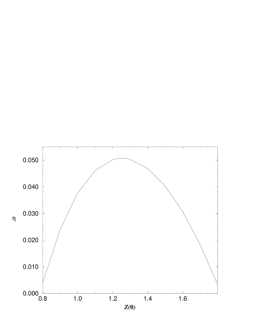
Figure 3: Plot of the anomalous dimension $\eta$ for various FPs, with fixed $A=0.8$, $B=0.5$, as a function of their normalization $Z(0)$. These are the transformations used in Ref. [6]. The maximum of the curve occurs at $Z(0)=1.25$ with $\eta=0.051$.

As explained earlier, this pattern is a consequence of the breaking of reparameterization symmetry. The line of equivalent FPs is converted into a line of non-equivalent FPs because only the most local ones can be adequately described by our approximation, being the rest quite distorted. Furthermore, the latter can be easily confused with some approximation of genuine non-local ones. And, as explained above, we take as a hint for locality the fact that a reminiscence of the line of FPs is present. That is, we take as the closest to the exact Wilson FP the one with an anomalous dimension which is first-order independent of $Z(0)$. For a given transformation (for fixed $A$ and $B$) there is only one point with that property.

Once we know how to compute the anomalous dimension given the RG transformations, we have to ask ourselves which are the most appropriate blockings. This is an old subject, which has been studied mainly on the lattice. For exact RG equations and their approximations it was addressed in the pioneering work of Ref. [3]. After it no much progress was achieved until Ref. [6], where a systematic search over different transformations was made and a proposal of “best” transformation was given, based on a reformulation of the principle of minimal sensitivity used in perturbation theory.

Unfortunately, this latter reference is incomplete in two important directions, as we have already outlined in the introduction. The first one is its poor calculation of the anomalous dimension, without taking into account the problem of the breaking of reparameterization invariance of the theory, thus making their results not quite trustworthy. The second problem is that their analysis did only half the way, leaving $\eta$ strongly dependent of one free parameter.

Nevertheless, we think the analysis of Ref. [6] is basically correct, as far as the general dependencies on $A$ and $B$ are concerned. That is, if a three dimensional plot of $\eta$ as a function of $A$ and $B$ is made, one identifies a sort of “hollow” around which $\eta$ presents a one-dimensional minimum whenever the hollow is crossed. To plot it, it is best to fixed one parameter, say $B$, and plot $\eta$ as a function of the other one, $A$ in our case. These kind of plots are shown in Fig. 4, whereas a sketch of the location of the hollow in the $A$–$B$ plane is presented in Fig. 5.

Figure 4: The anomalous dimension $\eta$ as a function of $A$ for $B=0.30$ (solid line), $B=0.40$ (dashed line) and $B=0.50$ (dotted line).

Figure 5: The “hollow” of $\eta$ in the $A$–$B$ plane.

We choose, as in Ref. [6], a minimal sensitivity criterion to select the transformations for which $\eta$ yields on the hollow. This should be the ones for which the derivative expansion converges the fastest. See Ref. [7] for an introduction of minimal sensitivity ideas.

Nevertheless, the strongest dependences of $\eta$ on the transformations occur along the hollow, not across it. Compare, for instance, a plot of different $\eta$’s along the hollow (Fig. 6) with Fig. 4 above. In fact, the reason which prevents us to 3d-plot $\eta$ versus the $A$–$B$ plane is that the quite different scales make it difficult to visually appreciate the details of the hollow.

Figure 6: The plot of $\eta$ along the hollow, parameterized by its $B$ value. This plot is to be compared with that of Fig. 4. Here the curve is much steeper.

We must then establish a criterion in order to keep only a small range of $B$ values if we wish to have a reasonable prediction for $\eta$. If not, it can take nearly any value we want, since, as it was already observed in Ref. [6], it grows nearly linearly along the hollow. The other parameter one has to fine-tune to obtain the FP, e.g., $\gamma\equiv f^{\prime}(0)$, behaves also in a similar fashion (see Fig. 7). For consistency with previous choices, the criterion we choose must be based in convergence properties of the derivative expansion. Clearly, one cannot focus on $\eta$, since it changes from $\eta=0$, imposed by the LPA, to a value close (hopefully) to the actual one. This is because it has to do with the newly added term, $Z(\varphi)$, which was not present previously. However, if the expansion converges sufficiently fast, the function $f(\varphi)$ obtained at second order must not be too different from the one obtained at lowest order. This is the criterion we propose: One should trust those FPs whose values of $\gamma$ are close to the same, unique, number obtained from the LPA. This selects the transformations around those with $A=0.53$ and $B=0.40$, with $\gamma=-0.229\,0$ (to be compared with $\gamma=-0.228\,6$ from the LPA). Its anomalous dimension is $\eta=0.042$. The FP action is plotted in Fig. 8.

Figure 7: The plot of $\gamma$ along the hollow, parameterized by its $B$ value.

Figure 8: The FP functions $f(\varphi)$ (solid line) and $Z(\varphi)$ (dashed line) for second order in the derivative expansion with $A=0.53$, $B=0.40$ and $Z(0)=1.31$.

Note that with this choice we hope to reproduce well the behavior of the FP action near $\varphi=0$. We do so following the common lore that this is the relevant part to reproduce if quantum fluctuations of the field are not very important, i.e., whenever $\eta$ is small. In fact, the whole idea would fail if the LPA was not sensible enough, which in turn is based on $\eta=0$ not being so crude an approximation. It is noteworthy, nonetheless, that there are other transformations which reproduce better than ours the asymptotic properties of $f(\varphi)$ but give quite worse results. For instance, in Fig. 9 we plot the function $f(\varphi)$ for the LPA, together with the chosen $A=0.53$, $B=0.40$ FP and with that from $A=0.21$, $B=0.70$. The last FP coincides quite well with the LPA one for $\varphi\to\infty$ but differs from it significantly for $\varphi\sim 0$, just the opposite behavior of ours. Nevertheless, our choice seem to give a better anomalous dimension ($\eta=0.042$ instead of $\eta=0.058$).

Figure 9: Comparison of the function $f(\varphi)$ from the LPA (solid line) with the second order ones corresponding to (1) $A=0.21$, $B=0.70$ (dashed line), which becomes similar to the previous one for large $\varphi$, but differs significantly from it for $\varphi\sim 0$; (2) $A=0.53$, $B=0.40$ (dotted line), which do not match with the first one for large $\varphi$, but coincides with it quite well for $\varphi\sim 0$.

Before finishing this section, we would like to insist that we have just presented a standard calculation within the derivative expansion up to second order, without any further approximation. The discussion above is focused on the set of transformations best suited for such a calculation. Without a clever choice, the expansion is poorly convergent and higher orders are necessary to provide the desired accuracy.

6.4 Ising universality class: critical indices

The computation of the eigenvalues is similar to that of the anomalous dimension $\eta$. We have two asymptotic free parameters $g_{1}$ and $h_{1}$ for a polynomially growing $g(\varphi)$ and $h(\varphi)$,

$$g(\varphi)\sim g_{1}\varphi^{\frac{d-2+\eta-2\lambda}{d+2-\eta}}+\cdots\quad\hbox{as $\varphi\to\infty$,}$$ (53)

$$h(\varphi)\sim h_{0}\varphi^{\frac{-4+2\eta-2\lambda}{d+2-\eta}}+h_{1}\varphi^{\frac{-8+2\eta-2\lambda}{d+2-\eta}}+\cdots\quad\hbox{as $\varphi\to\infty$,}$$

plus the eigenvalue $\lambda$ ($h_{0}$ is a parameter directly determined from $g_{1}$), but $Z_{2}$ symmetry imposes $g(0)=h^{\prime}(0)=0$ and the linearity of the eigenvalue Eq. (2) allows us to fix on more parameter, say $g^{\prime}(0)=1$. In this way the system gets determined and we encounter only a countable number of solutions. We discuss the three most relevant ones. We concentrate here on the FP with $A=0.53$, $B=0.40$, $d=3$, as we stated above.

The only relevant eigenvalue found gives $\nu=0.622$.

The second eigenvalue is not part of the physical spectrum, but corresponds to the redundant operator which generates the line of FPs in the exact case. In fact, its appearance is a crucial test of consistency of our method for calculating $\eta$. This is so because it must necessarily be marginal, otherwise it cannot connect two points which both of them are FPs of the same RG transformations. For exactly $A=.53$, $B=0.40$ and $Z(0)=1.31$ we obtain $\lambda=0.001$. A plot of this redundant eigenvalue for different $\eta$’s is given in Fig. 10. Note that for each $\eta$ there are two values of $\lambda$, corresponding to the two FPs which exist (cf. Figs. 2, 3). The eigenvalue vanishes only when there is a unique FP given $\eta$, i.e., when $\eta$ is approximately invariant under $Z(0)$.

Figure 10: The redundant eigenvalue $\lambda$ as a function of $\eta$ for $A=0.53$, $B=0.40$ and varying $Z(0)$.

Finally, we seek for the first irrelevant eigenvalue, which controls the first deviations to scaling. It gives $\omega=0.754$.

Together with the eigenvalues, there comes also their corresponding eigenvectors. As an example, we plot in Fig. 11 the one corresponding to the marginal redundant operator.

Figure 11: The marginal redundant eigenoperator for $A=0.53$, $B=0.40$ and $Z(0)=1.31$. The solid line corresponds to the function $f(\varphi)$, while the dashed one to $Z(\varphi)$. For display purposes, we have chosen the normalization $h(0)=1$, which gives $g^{\prime}(0)=-0.031$.

6.5 Accuracy

All figures given so far are significant. Such a precision is achieved because, ones the problem has been set up, one can push the numerical calculations sufficiently far to obtain a high accuracy (of even five or six digits). In fact, the main sources of errors are, on one hand, the problem introduced by different convergence properties of different transformations; and on the other, the poor knowledge of the corrections one may expect at higher orders.

The first problem can be turn to our favor. Once our criteria is accepted, there is only left the problem of to which accuracy we want $\gamma$ from the LPA be the same as the calculated at second order. Clearly, we expect the quantity to be corrected somehow at each order in the derivative expansion, so it is not sensible to ask for a terribly high coincidence. If we restrict ourselves to FPs with $\gamma$ three significant digits equal to the LPA value, then the anomalous dimension varies within the range $\eta=0.041\,9$–$0.042\,6$, thus providing us with an indication of the accuracy of our results. The eigenvalues are, nonetheless, far more insensitive, specially the relevant one. As an extreme example take, for instance, $A=0.21$, $B=0.70$, which gives $\nu=0.631$, $\omega=0.689$.

The main drawback of the whole framework, nevertheless, is its poor treatment of systematic errors introduced by the truncation of the expansion. In fact, there are, up to now, no methods to estimate the contribution from higher orders. It is amazing that the same feature that makes the technique so powerful (its no use of a small parameter like $\epsilon\equiv 4-d$ or the inverse number of fields $1/N$), also prevents us to make a thorough study of its errors, thus reducing the reliability of its conclusions.

Exact RG in this respect is special: in contradiction with what usually occurs, it happens to have the peculiarity that it is computationally quite simple, but its restrictions arrive in its deficient treatment of errors. We have not a clear way to control the size of next corrections within the derivative expansion, nor wee can evaluate how good our criterium for improving convergence is. This is the main problem of the method, not the computation itself.

6.6 Discussion

Table 1 contains a summary of our results, together with a comparison with results from the LPA and also from other methods (exact RG for the effective action and a combination of best known estimates [1]). It is remarkable that with exact RG computations one may obtain numbers quite close to the best known estimates, and with considerably less effort.

LPA Polchinski eff. action best known $\eta$ 0 0.042 0.054 0.035(3) $\nu$ $0.650$ 0.622 0.618 0.631(2) $\omega$ $0.656$ 0.754 0.897 0.80(4)

Table 1: The critical exponents $\eta$, $\nu$ and $\omega$ for (1) the LPA of Polchinski equation; (2) derivative expansion at second order of Polchinski equation; (3) derivative expansion at second order of the effective action RG equation [1]; (4) combination of best known estimates taken from Ref. [1].

We hope that the present paper serves to convince the reader that reported ambiguities in universal quantities computed with Polchinski equation [6, 18] do not constitute a problem, but rather can be turned to our favor. There is still open, nonetheless, the problem of how one can compute systematic errors, which is the reason that prevents exact RG methods to be totally competitive with the best existing techniques (Monte Carlo RG [19], $\epsilon$-expansion [20], …).

As a final comment we want to recall that exact RG methods seem to give always an anomalous dimension $\eta$ that increases from zero (LPA) to a value which is slightly above the best estimate; while the critical exponent $\nu$ goes the other way round, going form a high value from the LPA to another one which is probably a bit low. The exponent $\omega$ does not seem to oscillate around its actual value, but this may only reflect our poor knowledge of it. The apparent general behavior of $\eta$ and $\nu$ is, however, quite intriguing, because if it is really general then it may constitute a first step towards an accurate estimation of errors.

Appendix A Identity operator

It is known that, at any FP, there always exists an eigenoperator with eigenvalue $\lambda=d$, which is the highest dimensional operator of the theory. Let us briefly review the arguments that support it [21].

Let us take any FP action $S^{*}$ and consider perturbations with a set of operators ${\cal O}_{\alpha}$,

$$S=S^{*}+j_{\alpha}{\cal O}_{\alpha},$$ (54)

where $j_{\alpha}$ are some coupling constants. Implicit summation over repeated labels is understood throughout.

The partition function is then

$$Z=\int{\cal D}\phi\,e^{-S^{*}-j_{\alpha}{\cal O}_{\alpha}},$$ (55)

and we define the thermodynamic densities

$$M_{\alpha}\equiv\frac{1}{V}\frac{\partial}{\partial j_{\alpha}}\ln Z,$$ (56)

with $V$ the volume of the system (needed in order $M_{\alpha}$ to be an intensive quantity and, thus, defined in the thermodynamic limit).

After a RG transformation, the system is shrunk in all linear dimensions and new couplings $j^{\prime}_{\beta}$ are introduced,

$$V^{\prime}=e^{-d\tau}V,\qquad j^{\prime}_{\beta}=j^{\prime}_{\beta}(j_{\alpha}),$$ (57)

with the partition function kept invariant. The above defined densities thus transform to

$$M_{\alpha}=e^{-d\tau}\frac{\partial j^{\prime}_{\beta}}{\partial j_{\alpha}}\frac{1}{V^{\prime}}\frac{\partial}{\partial j^{\prime}_{\beta}}\ln Z\equiv e^{-d\tau}\frac{\partial j_{\beta}}{\partial j_{\alpha}}M^{\prime}_{\beta}.$$ (58)

Around a FP, the linearized RG transformations are precisely the matrix ${\cal R}_{\beta\alpha}\equiv\frac{\partial j^{\prime}_{\beta}}{\partial j_{\alpha}}$, with the right hand side evaluated at the FP. Therefore, using that, at a FP, $M^{\prime}_{\beta}=M_{\beta}$,

$${\cal R}_{\beta\alpha}M_{\beta}=e^{d\tau}M_{\alpha}.$$ (59)

The final result is, therefore, that the densities $\{M_{\alpha}\}$ form an eigenvector of the linearized RG transformations, with eigenvalue $\lambda=d$.

However, the above densities are expectation values of local operators and we may worry if all of them vanish. That this is not the case is due to the existence of the identity operator, whose expectation value is

$$<\hbox{\bf 1}>\equiv\frac{1}{V}\frac{\partial}{\partial j_{0}}\ln\int{\cal D}\phi\,e^{-S^{*}+j_{0}V}=1.$$ (60)

This completes the proof.

With Polchinski equation, one may also trivially show that the identity operator is always an eigenvector with eigenvalue $\lambda=d$ (just substitute $S=S^{*}+\int d^{d}x$ in Eq. (8) and use that $S^{*}$ is a FP).

In the derivative expansion we do not notice it because it is $g(\varphi)=h(\varphi)=0$. However, if the FP potential is $V_{FP}(\varphi)$ and its eigenperturbations $v(\varphi)$, then the linearized RG equation for the LPA may be rewritten as (cf. Eq. 26)

$$\lambda v=-2v^{\prime}V_{FP}^{\prime}+v^{\prime\prime}+dv-\frac{d-2}{2}\varphi v^{\prime},$$ (61)

with $\lambda=d$, $v=\hbox{constant}$, a trivial solution. At next order we have to solve

$$\lambda v = -2v^{\prime}V_{FP}^{\prime}+v^{\prime\prime}+Ah+dv-\frac{d-2+\eta}{2}\,\varphi v^{\prime},$$

$$\lambda h = -2V_{FP}^{\prime\prime}h^{\prime}-2v^{\prime}Z_{FP}^{\prime}-4V_{FP}^{\prime\prime}h-4v^{\prime\prime}Z_{FP}+4BV_{FP}^{\prime\prime}v^{\prime\prime}$$

$$\mbox{}+h^{\prime\prime}+4v^{\prime\prime}-\eta h-\frac{d-2+\eta}{2}\,\varphi h^{\prime}.$$

And, again, a trivial solution is

$$\lambda=d,\qquad v=\hbox{constant},\qquad h=0.$$ (63)

Appendix B Numerical methods

We explain in this appendix the numerical methods used at second order. The calculation of the LPA results can be inferred form them and, moreover, they are discussed elsewhere [2].

The FP is searched by shooting from the origin to some point $\varphi_{0}$ where we impose the asymptotic conditions valid for $\varphi_{0}\to\infty$, (cf. Eq. (6.3)),

$$\varphi_{0}\frac{f^{\prime}(\varphi_{0})-\frac{2-\eta}{2}}{f(\varphi_{0})-\frac{2-\eta}{2}\,\varphi_{0}}=\frac{d-2+\eta}{d+2-\eta},\qquad Z^{\prime}(\varphi_{0})=0.$$ (64)

Of course, these conditions cannot be imposed for finite $\varphi_{0}$, but we turn this fact to our advantage. We move $\varphi_{0}$ between 4 and 6, calculating $\eta$ and $\gamma$ at each step and we observed that the results stabilizes for the five or six significant figures at some point between 5 and 6. Thus it serves not only to check that the sub-leading asymptotic terms can be effectively discarded but also to check the accuracy of the overall numerical method.

Incidentally, all numbers quoted are obtained always with at least one significant digit more than shown, to make sure that the numerical errors are under control.

The computation is made with one normalization at a time, increasing it with finite amounts of 0.01. From the FPs so obtained, we keep the one with maximum $\eta$, as explained in Section 6. We check that this grid does not affect the results, within our accuracy. For instance, for the quoted $\eta=0.042$, $A=0.53$, $B=0.40$, we have: for $Z(0)=0.30$, $\eta=0.041\,966$; for $Z(0)=0.31$, $\eta=0.041\,985$; and for $Z(0)=0.32$, $\eta=0.041\,981$.

The scanning of the $A$–$B$ plane is made in a similar fashion (also with finite amounts of 0.01). To identify the hollow mentioned in Section 6 we fix first $B$ and obtain the FPs for different $A$, and choose the one with the minimum $\eta$ (see Fig. 4). Again, the grid should not be a great concern. Compare, for $B=0.40$: $A=0.52$, $\eta=0.041\,985\,1$; $A=0.53$, $\eta=0.041\,984\,8$; $A=0.54$, $\eta=0.041\,989\,1$.

Finally, the choice of a certain point within the hollow. This is a bit more difficult as computed quantities are far more sensitive to a variation within this line. As explained in Section 6, we take this as an indication of how far on can go with ones accuracy. We quote some representative numbers in Table 2, which are to be compare with $f^{\prime}(0)=-0.228\,60$ from the LPA.

$A$ $B$ $Z(0)$ $f^{\prime}(0)$ $\eta$ 0.55 0.39 1.31 $-0.230\,17$ $0.041\,3$ 0.53 0.40 1.31 $-0.228\,99$ $0.042\,0$ 0.52 0.41 1.32 $-0.228\,07$ $0.042\,6$ 0.49 0.42 1.33 $-0.227\,11$ $0.043\,3$

Table 2: Comparison of different FPs on the “hollow” (see Section 6). Recall that $f^{\prime}(0)=-0.288\,60$ within the LPA.

The computation of the eigenvalues is a quite easier problem, once the FP is determined (recall that now we are dealing with linear equations). Here we shoot from the origin (with $g^{\prime}(0)$ fix) and fine-tune the initial condition $h(0)$ and the eigenvalue $\lambda$, by imposing that the eigenfunctions $g(\varphi)$ and $h(\varphi)$, together with their derivatives, remain bounded. (This somehow bold asymptotic conditions suffice.) Of course, one has to repeat the above analysis to be sure that the results are independent of the numerical method and, in particular, of the point where the asymptotic conditions are imposed.

References

- [1] T.R. Morris, Phys. Lett. 329 (1994) 241
- [2] J. Comellas and A. Travesset, UB-ECM-PF-96-21, hep-th/9701028
- [3] T.L. Bell and K.G. Wilson, Phys. Rev. B 11 (1975) 3431
- [4] K.E. Newman and E.K. Riedel, Phys. Rev. B 30 (1984) 6615; G.R. Golner, Phys. Rev. B 33 (1986) 7863
- [5] J. Polchinski, Nucl. Phys. B 231 (1984) 269
- [6] R.D. Ball et. al., Phys. Lett. B 347 (1995) 80
- [7] P.M. Stevenson, Phys. Rev. D 23 (1981) 2916
- [8] J. Zinn-Justin, Quantum Field Theory and Critical Phenomena, Oxford Univ. Press (1993); T.R. Morris, Int. J. Mod. Phys. A 9 (1994) 2411
- [9] A. Hasenfratz and P. Hasenfratz, Nucl. Phys. B 270 (1986) 687; T.R. Morris, Nucl. Phys. B 458 (1996) 477
- [10] T.L. Bell and K.G. Wilson, Phys. Rev. B 10 (1974) 3935
- [11] J. Cardy, Scaling and Renormalization in Statistical Physics, Cambridge Univ. Press (1996)
- [12] K.G. Wilson and J. Kogut, Phys. Reports 12 (1974) 75
- [13] F.J. Wegner and A. Houghton, Phys. Rev. A 8 (1973) 401
- [14] F.J. Wegner, J. Phys. C 7 (1974) 2098
- [15] T.R. Morris, in RG96, hep-th/9610012
- [16] E.K. Riedel et al., Ann. Phys. 161 (1985) 178
- [17] M. D’Attanasio and T.R. Morris, Phys. Lett. B 378 (1996) 213
- [18] J. Comellas et al. Nucl. Phys. B 490 (1997) 653
- [19] C.F. Baillie et. al., Phys. Rev. B 45 (1992) 10438
- [20] J.C. Le Guillou and J. Zinn-Justin, Phys. Rev. B 21 (1980) 3977
- [21] M.E. Fisher and A. Nihat Berker, Phys. Rev. B 26 (1982) 2507