KEK-TH-518

TIT/HEP-369

May 1997

String Field Theory from IIB Matrix Model

Masafumi Fukuma¹⁾, Hikaru Kawai²⁾, Yoshihisa Kitazawa³⁾and Asato Tsuchiya^2)
1) Yukawa Institute for Theoretical Physics, Kyoto University,
Kitashirakawa Sakyo-ku, Kyoto 606-01, Japan

²⁾ National Laboratory for High Energy Physics (KEK),
Tsukuba, Ibaraki 305, Japan

³⁾ Department of Physics, Tokyo Institute of Technology,

Oh-okayama, Meguro-ku, Tokyo 152, Japan

We derive Schwinger-Dyson equations for the Wilson loops of a type IIB matrix model. Superstring coordinates are introduced through the construction of the loop space. We show that the continuum limit of the loop equation reproduces the light-cone superstring field theory of type IIB superstring in the large-N limit. We find that the interacting string theory can be obtained in the double scaling limit as it is expected.

1 Introduction

The recent development in our understanding of nonperturbative aspects of string theory has reinforced the connection between string theory and gauge theories[1][2][3]. It has been well known that the gauge theories can be obtained in the low energy limit of string theory. On the other hand the nonperturbative reformulation of superstring theory appears to be possible now in terms of the D-particles[4] or the D-instantons [5]. They are nothing but large-N (partially) reduced models of ten dimensional super Yang-Mills theory.

It has been long hoped that the gauge theories may be solvable in the large-N limit as a kind of string theory[6]. In gauge theories, the Wilson loops are the natural candidates to be identified with strings. They indeed obey the loop equations which resemble the Virasoro constraints in string theory. Hence the loop equations have been investigated in the hope of deriving the (light-cone) Hamiltonian of string theory[7]. The large-N reduced models have been originally invented in such a context[8] and the relation to bosonic string theory has been noted[9][10]. These hopes appear to be realizable now for ten dimensional super Yang-Mills theory in a most dramatic setting which involves the theory of gravitation and the unification of forces.

Our matrix model for type IIB superstring has the manifest $N=2$ super Poincare invariance in ten dimensions. It has the lowest dimensional constituents (D-instantons) and the highest symmetry of this class of the matrix models. We hope it will be most useful to investigate the nonperturbative aspects of superstring theory. The related models and the possible extensions have also been proposed [12][13][14][15][16][17][18]. Qualitatively reasonable results have already been obtained at long distance by the matrix models when we investigate the interactions between the D-strings at the one loop level. However the standard folklore suggests that we may need to sum up all planar diagrams of the matrix models even to obtain free strings. Therefore we need to solve the theory in the large-N limit. Since we know a possible solution (superstring) to this question, this task is not inconceivable. Our aim of this paper is in fact to derive the light-cone field theory of Green, Schwarz and Brink[11] for type IIB superstring from a matrix model[5].

The only successful string field theories so far are formulated in the light-cone gauge. In this respect they may not be effective to study nonperturbative aspects of string theory. However our motivation to derive the light-cone superstring field theory from the matrix model here is to prove that the matrix model reproduces the standard string perturbation theory.

In section 2, we introduce the Wilson loops as the operators which create and annihilate strings (string fields). The string coordinates are introduced through the Wilson loops. We then discuss the continuum limit of the differential operators in the loop space. In section 3, we set up the loop equations for the Wilson loops by using the Schwinger-Dyson equations. We demonstrate that the loop equations reduce to that of free supersrting Hamiltonian in the large-N limit. We also explain that the structure of the cubic light-cone Hamiltonian of superstring naturally appears from the matrix model. In section 4, we construct a general proof of our assertion that the IIB matrix model reproduces the light-cone superstring field theory in the double scaling limit. We construct supercharges of the matrix model in the loop space and show that they agree with those of superstring theory. The proof is based on the power counting and the symmetry arguments. We conclude in section 5 with discussions.

One of the crucial issues of the matrix model approach is to reproduce the standard string perturbation theory. We are successful in this respect since we have derived light-cone Hamiltonian of superstring from the matrix model. Therefore we have proven our previous conjecture that our matrix model is indeed a nonperturbative formulation of type IIB superstring theory.

2 Strings and the Wilson loops

We recall our matrix model action[5] which is a large-N reduced model of ten dimensional super Yang-Mills theory:

$$S=-{1\over g^{2}}Tr({1\over 4}[A_{\mu},A_{\nu}][A^{\mu},A^{\nu}]+{1\over 2}\bar{\psi}\Gamma^{\mu}[A_{\mu},\psi]),$$ (2.1)

where $\psi$ is a ten dimensional Majorana-Weyl spinor field, and $A_{\mu}$ and $\psi$ are $N\times N$ Hermitian matrices. We have interpreted some of the classical solutions of this action as D-strings and shown that they indeed interact in a consistent way with this interpretation at long distance.

We have also proposed that the Wilson loops are the creation and annihilation operators for strings[5]. The Wilson loops can wind many times around the world even in the reduced models which have only few (even single) points in the universe. If we consider the T-duality, the winding numbers can be reinterpreted as the momentum. Based on these reasonings, we consider the following regularized Wilson loops:

$$w(C) = Tr[v(C)],$$

$$v(C) = \prod_{n=1}^{M}U_{n},$$

$$U_{n} = exp\{i\epsilon(k_{n}^{\mu}A_{\mu}+\bar{\lambda}_{n}\psi)\}.$$ (2.2)

Here $k_{n}^{\mu}$ are momentum densities distributed along $C$, and we have also introduced the fermionic sources $\lambda_{n}$ . $\epsilon$ in the argument of the exponential is a cutoff factor. As we will see in the subsequent sections, $\epsilon$ can be regarded as a lattice spacing of the worldsheet. We therefore call $\epsilon\rightarrow 0$ limit the continuum limit. We may also Fourier transform the Wilson loop from the momentum space $k^{\mu}_{n}$ to the real space $x^{\mu}_{n}$.

In the next section, we consider the continuum limit of the Wilson loops. As a preparation we study the differential operators in the loop space and the operator insertions into the Wilson loops in the remaining part of this section . Let us consider the operator insertion of $A_{\mu}$ between the $n-$th and the $(n+1)-$th links:

$$U_{n}A_{\mu}U_{n+1}.$$ (2.3)

To the leading order of $\epsilon$, it is equivalent to a simple differential operator in the loop space:

$${\partial\over\partial i\epsilon k^{\mu}_{n}}U_{n}U_{n+1}$$ (2.4)

$$= U_{n}\int_{0}^{1}dtexp\{-i\epsilon t(k^{\nu}_{n}A_{\nu}+\bar{\lambda}_{n}\psi)\}A_{\mu}exp\{i\epsilon t(k^{\nu}_{n}A_{\nu}+\bar{\lambda}_{n}\psi)\}U_{n+1}$$

$$= U_{n}(A_{\mu}-{i\epsilon\over 2}[k^{\nu}_{n}A_{\nu}+\bar{\lambda}_{n}\psi,A_{\mu}]+\cdots)U_{n+1}.$$

However eqs.(2.3) and (2.4) differ from each other at the next order of $\epsilon$ by the commutators. The commutators such as $[A_{\mu},A_{\nu}]$ can be expressed by differential operators in the loop space as follows:

$$({\partial\over\partial i\epsilon k^{\mu}_{n}}-{\partial\over\partial i\epsilon k^{\mu}_{n+1}})({\partial\over\partial i\epsilon k^{\nu}_{n}}+{\partial\over\partial i\epsilon k^{\nu}_{n+1}})U_{n}U_{n+1}$$ (2.5)

$$= U_{n}([A_{\mu},A_{\nu}]+\cdots)U_{n+1}.$$

Therefore the leading commutators in eq.(2.4) can be expressed in terms of differential operators in the loops space. So the operator insertion (2.3) can be expressed by a differential operator in the loop space up to $O(\epsilon)$. The remaining commutators which involve three matrix fields can be expressed by differential operators in an analogous way if we consider three neighboring links. In this way in principle any operator insertion into the Wilson loop can be expressed by an infinite series of local differential operators in the loop space.

We also consider the differentiation of the Wilson loops by the matrix valued fields. The differentiation of the link variable by $A_{\mu}$ is given by.

$${\partial\over\partial A^{\alpha}_{\mu}}U_{n}$$ (2.6)

$$= i\epsilon k^{\mu}_{n}\int_{0}^{1}dtexp\{i\epsilon t(k^{\nu}_{n}A_{\nu}+\bar{\lambda}_{n}\psi)\}t^{\alpha}exp\{-i\epsilon t(k^{\rho}_{n}A_{\rho}+\bar{\lambda}_{n}\psi)\}U_{n}$$

$$= i\epsilon k^{\mu}_{n}(t^{\alpha}+{i\epsilon\over 2}[k^{\nu}_{n}A_{\nu}+\bar{\lambda}_{n}\psi,t^{\alpha}]+\cdots)U_{n}.$$

Here $t^{\alpha}$ denotes the generators of the gauge group $U(N)$. Obviously the leading term is the multiplication by $i\epsilon k^{\mu}_{n}t^{\alpha}$. Again the remaining terms can be expressed by some infinite series of differential operators.

Finally we make a comment on the universality of the differential operators in the loop space. What we are interested in is the continuum limit such as

$$y_{n+1}-y_{n}\sim\epsilon y^{\prime}(\sigma),\;{\partial\over\epsilon\partial y_{n}}\sim{\delta\over\delta y(\sigma)}.$$ (2.7)

At first glance it seems that the differential operators which correspond to multi-commutators of the matrix fields are suppressed by some powers of $\epsilon$ in the continuum limit. However we cannot simply say that they do not contribute in the continuum theory because they can renormalize the operators which survive in the naive continuum limit. We may draw an analogy with the quantum field theory on the lattice here. The lattice action may be expanded formally in terms of the lattice spacing $a$. Although the operators which are suppressed by the powers of $a$ formally vanish in the continuum, we cannot simply neglect them because they may renormalize the relevant operators. In fact we can write down many lattice actions which possess the identical continuum limit. Although they are not unique, the continuum limit is universal which enables us to define a unique continuum theory. We assume a similar universality on the differential operators in the loop space. Namely we expect that the differential operators we consider in the subsequent sections represent unique quantities in the continuum limit although they are certainly not unique with finite $\epsilon$.

3 Loop equations

In this section, we often show only the naive leading terms in the loop equations. As we have explained in the last section, it should be understood that they simply represent the universality classes of the differential operators. The basic equations we consider here are the following Schwinger-Dyson equations:

$$\int dAd\psi{\partial\over\partial A_{\mu}^{\alpha}}\{Tr[t^{\alpha}v(C^{1})]w(C^{2})w(C^{3})\cdots w(C^{l})exp(-S)\}=0,$$ (3.1)

$$\int dAd\psi{\partial\over\partial\psi^{\alpha}}\{Tr[t^{\alpha}v(C^{1})]w(C^{2})w(C^{3})\cdots w(C^{l})exp(-S)\}=0.$$ (3.2)

We also need an equation which is related to the local reparametrization invariance of the Wilson loop:

$$\{(k^{\mu}_{n}+k^{\mu}_{n+1})({\partial\over\epsilon\partial k^{\mu}_{n+1}}-{\partial\over\epsilon\partial k^{\mu}_{n}})+(\bar{\lambda}_{n}+\bar{\lambda}_{n})({\partial\over\epsilon\partial\bar{\lambda}_{n+1}}-{\partial\over\epsilon\partial\bar{\lambda}_{n}})+\cdots\}w(C)=0.$$ (3.3)

It is easy to check that the above expression is satisfied up to $O(\epsilon)$ without the terms expressed by the dots. Since the $O(\epsilon^{2})$ contribution is commutators of three matrix fields, it can be expressed as differential operators in the loop space as it is explained in the previous section. It is clear now that we can satisfy this identity by iterating such a procedure. This identity implies the standard local reparametrization invariance of the Wilson loop in the continuum limit.

By multiplying $\frac{1}{2}(k^{\mu}_{1}+k^{\mu}_{M})$ to eq.(3.1), we find

$$\{-{3\over 2g^{2}N\epsilon^{2}}\Delta_{M}({\partial\over\epsilon\partial k})^{2}-i{1\over g^{2}N\epsilon}\hat{k}_{\mu M}\Delta_{M}({\partial\over\epsilon\partial\bar{\lambda}})\Gamma^{0}\Gamma^{\mu}{\partial\over\epsilon\partial\bar{\lambda}_{M}}\}<w(C^{1})w(C^{2})\cdots w(C^{l})>$$ (3.4)

$$+{1\over N}\sum_{j=1}^{M}\hat{k}_{\mu M}\hat{k}_{j}^{\mu}<Tr[\prod_{n=j+1}^{M}U_{n}]Tr[\prod_{m=1}^{j}U_{m}]w(C^{2})\cdots w(C^{l})>$$

$$+{1\over N}\sum_{b=2}^{l}\sum_{j=1}^{M^{b}}\hat{k}_{\mu M}\hat{k}_{j}^{\mu b}<Tr[\prod_{n=j+1}^{M^{b}}U^{b}_{n}v(C^{1})\prod_{m=1}^{j}U^{b}_{m}]w(C^{2})\cdots\check{w}(C^{b})\cdots w(C^{l})>$$

$$= 0,$$

where $\check{w}(C^{b})$ implies the absence of the Wilson loop $w(C^{b})$, and we have also introduced the notations $\Delta_{n}(y)\equiv y_{n+1}-y_{n}$ and $\hat{y}_{n}\equiv{1\over 2}(y_{n}+y_{n+1})$.

On the other hand from eq.(3.2), we obtain

$${i\over g^{2}N\epsilon}\Delta_{M}({\partial\over\epsilon\partial k^{\mu}})\Gamma^{\mu}({\partial\over\epsilon\partial\bar{\lambda}_{M}}+{\partial\over\epsilon\partial\bar{\lambda}_{1}})<w(C^{1})w(C^{2})\cdots w(C^{l})>$$ (3.5)

$$+{1\over N}\sum_{j=1}^{M}\hat{\lambda}_{j}<Tr[\prod_{n=j+1}^{M}U_{n}]Tr[\prod_{m=1}^{j}U_{m}]w(C^{2})\cdots w(C^{l})>$$

$$+{1\over N}\sum_{b=2}^{l}\sum_{j=1}^{M^{b}}\hat{\lambda}_{j}^{b}<Tr[\prod_{n=j+1}^{M^{b}}U^{b}_{n}v(C^{1})\prod_{m=1}^{j}U^{b}_{m}]w(C^{2})\cdots\check{w}(C^{b})\cdots w(C^{l})>$$

$$= 0.$$

In order to make the connections with the light-cone string field theory, we consider the configurations of the Wilson loops which possess the identical light-cone time $x^{+}$. Namely we perform the Fourier transformations of the Wilson loop from $k^{-}_{n}$ to $x^{+}_{n}$ and consider such configurations that $x^{+}_{n}=x^{+}$ for all the strings. We may also consider a group of the Wilson loops at $x^{+}=-\infty$ which represent a particular initial state. Strings which are created by the Wilson loops at $x^{+}=-\infty$ evolve in time and after splitting and joining they are eventually terminated by the Wilson loops at $x^{+}$. This is the setting of our problem which is illustrated in Fig. 1.

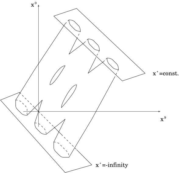
Figure 1: The setting of our problem. We consider the configurations of the Wilson loops which possess the identical light-cone time $x^{+}$. We also consider a group of the Wilson loops at $x^{+}=-\infty$ which represent a particular initial state.

Our strategy is to derive the light-cone Hamiltonian which governs the evolution of the strings from the loop equation. We can also put $k^{+}_{n}=1$ on the light-cone by using the reparametrization invariance of the Wilson loop. The fermionic variables $\lambda$ can be decomposed into $8_{s}$ and $8_{c}$ representations of $SO(8)$ as $\lambda_{a}$ and $\lambda_{\dot{a}}$. We eliminate $\lambda_{\dot{a}}$ and its conjugate $\theta_{\dot{a}}$ by using the loop equation (3.5) just like eliminating the half of the fermionic degrees of freedom in the light-cone field theory by using the equation of motion.

Our matrix model action can be rewritten as follows in the $SO(8)$ decomposition:

$$S = -{1\over g^{2}}Tr({1\over 4}[A_{\mu},A_{\nu}][A^{\mu},A^{\nu}]$$ (3.6)

$$+{1\over 2}(\sqrt{2}\psi_{{a}}[A^{+},\psi_{{a}}]-\psi_{a}\gamma^{i}_{{a}\dot{a}}[A_{i},\psi_{\dot{a}}]-\psi_{\dot{a}}\gamma^{i}_{\dot{a}{a}}[A^{i},\psi_{{a}}]+\sqrt{2}\psi_{\dot{a}}[A^{-},\psi_{\dot{a}}])).$$

We recall that the coupling constant of this model $g$ possesses the dimension of length squared since we identify the diagonal elements of $A_{\mu}$ as the spacetime coordinate in the semiclassical region.

In the light-cone setting we just explained, the loop equation (3.4) becomes as follows:

$$\hat{k}^{-}_{M}<w(C^{1})w(C^{2})\cdots w(C^{l})>$$

$$= Z^{-1}\{((\hat{k}^{i}_{M})^{2}+{3\over 2g^{2}N\epsilon^{2}}(\Delta_{M}(x^{i}))^{2}-i{\sqrt{2}\over g^{2}N}{\Delta_{M}(\theta_{a})\over\epsilon}\hat{\theta_{a}}_{M}$$

$$-{i\over g^{2}N\epsilon}\hat{k}^{i}_{M}\gamma^{i}_{a\dot{a}}(\Delta_{M}(\theta_{\dot{a}})\hat{\theta_{a}}_{M}+\Delta_{M}(\theta_{a})\hat{\theta_{\dot{a}}}_{M}))<w(C^{1})w(C^{2})\cdots w(C^{l})>$$

$$+{1\over N}\sum_{j=1}^{M-1}\hat{k}_{\mu M}\hat{k}^{\mu}_{j}<Tr[\prod_{n=j+1}^{M}U_{n}]Tr[\prod_{m=1}^{j}U_{m}]w(C^{2})\cdots w(C^{l})>$$

$$+{1\over N}\sum_{b=2}^{l}\sum_{j=1}^{M^{b}}\hat{k}_{\mu M}\hat{k}_{j}^{\mu b}<Tr[\prod_{n=j+1}^{M^{b}}U^{b}_{n}v(C^{1})\prod_{m=1}^{j}U^{b}_{m}]w(C^{2})\cdots\check{w}(C^{b})\cdots w(C^{l})>\},$$

where $Z=2(1+{i\over\sqrt{2}g^{2}N\epsilon}\Delta_{M}(\theta_{\dot{a}})\hat{\theta}_{\dot{a}M})$. We have also introduced conjugate variables $x^{\mu}_{n}=i{\partial\over\partial\epsilon k_{n\mu}}$ and $\theta_{n}\equiv{\partial\over\partial\epsilon\lambda_{n}}$.

In this equation, we have separated the minimal string contribution $(j=M)$ from the third line of the right-hand side of the equation which represents the splitting of the string and it is combined into the free Hamiltonian of the string. The string of vanishing length has $w(C)=Tr\,1=N$. The Wilson loop of a string with finite length cannot have the magnitude of $O(N)$ because of the conservation of the light-cone momentum $p^{+}$ and the large-N factorization. In fact the loop equation (LABEL:regloop) implies that its magnitude is of $O(1)$.

Since we put $k^{+}_{n}=1$, the total length of the string should be proportional to the total light-cone momentum $p^{+}=M\epsilon$. We note that the string coupling constant which governs the strength of the splitting and joining of strings is proportional to $1/N$ as expected. The string interaction conserves the bosonic and fermionic momentum densities $k_{n}$ and $\lambda_{n}$ locally. If we let $N\rightarrow\infty$ in eq.(LABEL:regloop) before taking $\epsilon\rightarrow 0$, the interaction terms can be neglected. Hence we find that a free string theory is obtained in the large-N limit.

We can eliminate $\lambda_{\dot{a}}$ and $\theta_{\dot{a}}$ from eq.(LABEL:regloop) iteratively by using the following loop equations which are obtained from eq.(3.5):

$$\hat{\theta}_{\dot{a}M}<w(C^{1})w(C^{2})\cdots w(C^{l})>$$ (3.8)

$$= {g^{2}N\over 2}({\Delta_{M}(x^{i})\over\epsilon}\gamma^{i}_{a\dot{a}})^{-1}\{\hat{\lambda}_{aM}<w(C^{1})w(C^{2})\cdots w(C^{l})>$$

$$+{1\over N}\sum_{j=1}^{M-1}\hat{\lambda}_{aj}<Tr[\prod_{n=j+1}^{M}U_{n}]Tr[\prod_{m=1}^{j}U_{m}]w(C^{2})\cdots w(C^{l})>$$

$$+{1\over N}\sum_{b=2}^{l}\sum_{j=1}^{M^{b}}\hat{\lambda}_{aj}^{b}<Tr[\prod_{n=j+1}^{M^{b}}U^{b}_{n}v(C^{1})\prod_{m=1}^{j}U^{b}_{m}]w(C^{2})\cdots\check{w}(C^{b})\cdots w(C^{l})>\},$$

and

$$\hat{\lambda}_{\dot{a}M}<w(C^{1})w(C^{2})\cdots w(C^{l})>$$ (3.9)

$$= ({2\sqrt{2}\over g^{2}N}{\Delta_{M}(x^{-})\over\epsilon}\hat{\theta}_{\dot{a}M}+{2\over g^{2}N}{\Delta_{M}(x^{i})\over\epsilon}\gamma^{i}_{\dot{a}a}\hat{\theta}_{aM})<w(C^{1})w(C^{2})\cdots w(C^{l})>$$

$$-{1\over N}\sum_{j=1}^{M-1}\hat{\lambda}_{\dot{a}j}<Tr[\prod_{n=j+1}^{M}U_{n}]Tr[\prod_{m=1}^{j}U_{m}]w(C^{2})\cdots w(C^{l})>$$

$$-{1\over N}\sum_{b=2}^{l}\sum_{j=1}^{M^{b}}\hat{\lambda}_{\dot{a}j}^{b}<Tr[\prod_{n=j+1}^{M^{b}}U^{b}_{n}v(C^{1})\prod_{m=1}^{j}U^{b}_{m}]w(C^{2})\cdots\check{w}(C^{b})\cdots w(C^{l})>.$$

Let us concentrate on the free propagation part of the string first. Although the large-N limit of the loop equation (LABEL:regloop) contains not only quadratic terms but also nonlinear terms, it is reduced to the following simple Hamiltonian in the continuum limit:

$$p^{-}=\int_{0}^{p^{+}}d\sigma{1\over 2}\{ck(\sigma)^{i}k(\sigma)^{i}+c^{\prime}\beta(x^{\prime}_{i}(\sigma))^{2}-ic^{\prime\prime}{\beta}\theta_{a}^{\prime}(\sigma)\theta_{a}(\sigma)-ic^{\prime\prime\prime}\lambda_{a}(\sigma)^{\prime}\lambda_{a}(\sigma)\},$$ (3.10)

where $\beta\equiv 1/g^{2}N$. It is because the only effect of the nonlinear operators in the continuum limit is the renormalization of the coefficients of the quadratic operators since they are suppressed by the powers of $\epsilon$. In particular $\lambda_{a}^{\prime}\lambda_{a}$ term is generated by the renormalization effect after eliminating $\theta_{\dot{a}}$ variables as it will be demonstrated shortly. As it will be shown in the next section, the form of the free light-cone Hamiltonian in the loop space is fixed uniquely by the power counting and the $N=2$ supersymmtery.

This Hamiltonian is identical to that of type IIB superstring theory[11] if $\lambda_{a}(\sigma)$ and $\theta_{a}(\sigma)$ are rescaled appropriately and rotated by a complex phase factor $\eta=exp({i\pi\over 4})$ as follows:

$$\lambda_{a}(\sigma)\rightarrow\eta\lambda_{a}(\sigma),~{}\theta_{a}(\sigma)\rightarrow\eta^{*}\theta_{a}(\sigma).$$ (3.11)

We elaborate more on this point in connection with the supercharges in the next section.

The string tension of this action eq.(3.10) is found to be $(\alpha^{\prime})^{2}\sim 1/\beta=g^{2}N$ which is again the standard combination to be held fixed in the large-N limit. Since $g$ has the dimension of the square of length, such an identification is consistent. Therefore we have obtained the standard light-cone Hamiltonian of free type IIB superstring in the large-N limit. In particular our type IIB matrix model is shown to possess the identical spectrum with free type IIB superstring in the large-N limit.

We now explain how the nonlinear operators renormalize the quadratic free string propagator by concrete examples. Since they involve $\theta_{\dot{a}}$, we need to eliminate it iteratively by using eq.(3.8). Let us consider the naive leading contribution in eq.(3.8):

$$\theta_{\dot{a}}<w(C)>={x_{i}^{\prime}(\sigma)\gamma^{i}_{\dot{a}a}\over(x_{i}^{\prime}(\sigma))^{2}}{g^{2}N\over 2}\lambda_{a}(\sigma)<w(C)>.$$ (3.12)

We assume first that a quadratic Hamiltonian such as eq.(3.10) correctly describes the free propagation of the Wilson loops of the matrix model. This assumption can be justified by showing that the nonlinear terms are indeed negligible in the continuum limit except for finite renormalization of the quadratic terms. Since we are dealing with free two dimensional field theories, we can utilize standard techniques of conformal field theory to estimate the effects of the nonlinear terms. We note that the $(x_{i}^{\prime}(\sigma))^{2}$ is of $1/\epsilon^{2}$ since we have a cutoff length $\epsilon$. So we may expand $(x_{i}^{\prime}(\sigma))^{2}=1/\alpha\epsilon^{2}+:(x_{i}^{\prime}(\sigma))^{2}:$ where $:y:$ denotes the normal ordered operator constructed out of $y$. $\alpha$ in the denominator is a quantity proportional to $\sqrt{\beta}$ on the dimensional grounds.

In this way, the left-hand side of the eq.(3.12) becomes

$$\epsilon^{2}{\alpha\over{2}\beta}x_{i}^{\prime}(\sigma)\gamma^{i}_{\dot{a}a}(1-\epsilon^{2}\alpha:(x_{i}^{\prime}(\sigma))^{2}:+\cdots)\lambda_{a}(\sigma)<W(C)>.$$ (3.13)

In principle we can eliminate $\theta_{\dot{a}}(\sigma)$ in eq.(LABEL:regloop) through this procedure, and we obtain many terms with various powers of $\epsilon$. However as we discuss in the next section the powers of $\epsilon$ can be understood in a simple dimensional analysis. We can assign the standard two dimensional canonical dimensions to the operators. The quadratic part of the light-cone Hamiltonian has the canonical dimension of two, and as we will see in the next section, operators with lower dimensions do not appear because of the $N=2$ supersymmetry. Therefore we can show that the nonlinear terms of the light-cone Hamiltonian is indeed irrelevant in the continuum limit except for finite renormalizations of the quadratic terms.

Finally we consider the string interactions. In principle we can evaluate the Hamiltonian $k^{-}_{n}$ by iteratively using eqs.(3.3), (LABEL:regloop), (3.8) and (3.9) to eliminate the operators $\frac{x^{-}_{n+1}-x^{-}_{n}}{\epsilon}$, $\theta_{n\dot{a}}$ and $\lambda_{n\dot{a}}$ in the right-hand side of eq.(LABEL:regloop). In this procedure, various interaction terms of order $1/N^{k}$ are generated, which represent processes where the $k+2$ strings interact at one point i.e. $(k+2)-$Reggeon vertices. However we will discuss in the next section that these interactions are completely controllable again by an analysis based on the symmetries and a power counting of $\epsilon$ at the interaction points.

4 N=2 supersymmetry and general proof

In this section, we give a general proof of our assertion in the previous sections by using a power counting and a symmetry analysis based on the $N=2$ supersymmetry, $SO(8)$ invariance and the parity symmetry on the string worldsheet.

4.1 Power counting and parity symmetry

In order to perform a power counting for $\epsilon$, we first introduce a mass dimension on the worldsheet through the relation $[\epsilon]=-1$ and determine the dimension of each field. By demanding the IIB matrix model action (3.6) to be dimensionless, we obtain

$$[A^{i}]=0,\>[A^{+}]=-[A^{-}],\>[A^{+}]=-2[\psi_{a}]\>\mbox{and}\>[A^{-}]=-2[\psi_{\dot{a}}].$$ (4.1)

From the definition of the Wilson loop (2.2), we also read off the relations

$$[k^{+}_{n}]+[A^{-}]=1,$$

$$[k^{-}_{n}]+[A^{+}]=1,$$

$$[k^{i}_{n}]+[A^{i}]=1,$$

$$[\lambda_{na}]+[\psi_{a}]=1,$$

$$[\lambda_{n\dot{a}}]+[\psi_{\dot{a}}]=1.$$ (4.2)

Noting that we should set $[k^{+}_{n}]$ to be zero since $k^{+}_{n}=1$ in our light-cone setting, we can determine the dimensions of all quantities as follows:

$$[k^{+}_{n}]=0,\>[k^{-}_{n}]=2,\>[k^{i}_{n}]=1,\>[\lambda_{na}]=\frac{1}{2},\>[\lambda_{n\dot{a}}]=\frac{3}{2},$$

$$[x^{+}_{n}]=-1,\>[x^{-}_{n}]=1,\>[x^{i}_{n}]=0,\>[\theta_{na}]=\frac{1}{2},\>[\theta_{n\dot{a}}]=-\frac{1}{2},$$

$$[A^{+}]=-1,\>[A^{-}]=1,\>[A^{i}]=0,\>[\psi_{a}]=\frac{1}{2},\>[\psi_{\dot{a}}]=-\frac{1}{2},$$ (4.3)

where $x^{\mu}_{n}=i\frac{1}{\epsilon}\frac{\partial}{\partial k_{n\mu}}$ and $\theta_{n}=\frac{1}{\epsilon}\frac{\partial}{\partial\lambda_{n}}$.

Next we define a symmetry which corresponds to the parity on the string worldsheet. It is seen easily that the IIB matrix model action (2.1) is formally invariant under the following transformation:

$$A_{\mu}\rightarrow A_{\mu}^{t},$$

$$\psi\rightarrow-i\psi^{t}.$$ (4.4)

This transformation flips the direction of the Wilson loop in the following way:

$$w(C)=Tr(P\prod^{M}_{n=1}e^{i\epsilon(k^{\mu}_{n}A_{\mu}+\bar{\lambda}_{n}\psi)})\rightarrow Tr(P\prod^{M}_{n=1}e^{i\epsilon(k^{\mu}_{M+1-n}A_{\mu}-i\bar{\lambda}_{M+1-n}\psi)}).$$ (4.5)

Therefore our theory has a symmetry under the transformation

$$k^{\mu}_{n}\rightarrow k^{\mu}_{M+1-n},$$

$$\lambda_{n}\rightarrow i\lambda_{M+1-n},$$ (4.6)

which we identify with the worldsheet parity. We also obtain the parity transformation for the dual variables $x^{\mu}_{n}$ and $\theta_{n}$:

$$x^{\mu}_{n}\rightarrow x^{\mu}_{M+1-n},$$

$$\theta_{n}\rightarrow-i\theta_{M+1-n}.$$ (4.7)

4.2 $N=2$ supersymmetry

As is discussed in [5], the IIB matrix model possesses the $N=2$ supersymmetry:

$$\delta^{(1)}\psi = \frac{i}{2}[A_{\mu},A_{\nu}]\Gamma^{\mu\nu}\varepsilon,$$

$$\delta^{(1)}A_{\mu} = i\bar{\varepsilon}\Gamma_{\mu}\psi,$$ (4.8)

and

$$\delta^{(2)}\psi = \sqrt{2}\xi,$$

$$\delta^{(2)}A_{\mu} = 0.$$ (4.9)

We can determine the dimensions and parities of the parameters $\varepsilon$ and $\xi$ by comparing the both sides of eqs.(4.8) and (4.9) respectively,

$$[\varepsilon_{a}]=[\xi_{a}]=\frac{1}{2},\>[\varepsilon_{\dot{a}}]=[\xi_{\dot{a}}]=-\frac{1}{2},$$

$$\varepsilon_{a}\rightarrow i\varepsilon_{a},\>\varepsilon_{\dot{a}}\rightarrow i\varepsilon_{\dot{a}},$$

$$\xi_{a}\rightarrow-i\xi_{a},\>\xi_{\dot{a}}\rightarrow-i\xi_{\dot{a}}.$$ (4.10)

This fixes the dimensions and parities of the supercharges $Q^{1}$ and $Q^{2}$ since $\varepsilon_{a}Q^{1}_{a}+\varepsilon_{\dot{a}}Q^{1}_{\dot{a}}+\xi_{a}Q^{2}_{a}+\xi_{\dot{a}}Q^{2}_{\dot{a}}$ generates the transformations (4.8) and (4.9):

$$[Q^{1}_{a}]=[Q^{2}_{a}]=-\frac{1}{2},\>[Q^{1}_{\dot{a}}]=[Q^{2}_{\dot{a}}]=\frac{1}{2},$$ (4.11)

$$Q^{1}_{a}\rightarrow-iQ^{1}_{a},\>Q^{1}_{\dot{a}}\rightarrow-iQ^{1}_{\dot{a}},$$

$$Q^{2}_{a}\rightarrow iQ^{2}_{a},\>Q^{2}_{\dot{a}}\rightarrow iQ^{2}_{\dot{a}}.$$ (4.12)

Here we note that eqs.(4.11) and (4.12) are consistent with the anti-commutation relations

$$\{Q^{1},Q^{1}\}=0,\>\{Q^{2},Q^{2}\}=0,$$

$$\{Q^{1}_{a},Q^{2}_{b}\}=2P^{+}\delta_{ab},$$

$$\{Q^{1}_{a},Q^{2}_{\dot{a}}\}=\sqrt{2}P^{i}\gamma^{i}_{a\dot{a}},\>\{Q^{1}_{\dot{a}},Q^{2}_{a}\}=\sqrt{2}P^{i}\gamma^{i}_{\dot{a}a},$$

$$\{Q^{1}_{\dot{a}},Q^{2}_{\dot{b}}\}=2H\delta_{\dot{a}\dot{b}}.$$ (4.13)

4.3 Free parts of supercharges and Hamiltonian

The supercharges $Q^{1}$ and $Q^{2}$ can be expressed as differential operators on the loop space using the Ward identities. In principle we can eliminate the operators $k^{-}_{n}$, $\frac{x^{-}_{n+1}-x^{-}_{n}}{\epsilon}$, $\lambda_{n\dot{a}}$ and $\theta_{n\dot{a}}$ by repeatedly using the loop equations and the reparametrization invariance as is discussed for $k^{-}_{n}$ in the previous section. Note that we obtain interaction terms through this procedure. However as we will see just below, the forms of their continuum limit are completely determined by the dimension, parity and $SO(8)$ invariance. First we concentrate on free parts of the supercharges $Q^{1}$ and $Q^{2}$ i.e. consider only the leading contribution of the $1/N$ expansion. By using the power counting, eqs.(4.3) and (4.11), $SO(8)$ invariance and the parity symmetry, eqs.(4.6), (4.7) and (4.12), we can deduce the following forms of free supercharges in the $\epsilon\rightarrow 0$ limit:

$$Q^{1}_{free\,a}=\int d\sigma a_{1}\theta_{a}(\sigma),$$

$$Q^{2}_{free\,a}=\int d\sigma a_{2}\lambda_{a}(\sigma),$$

$$Q^{1}_{free\,\dot{a}}=\int d\sigma(b_{1}x^{\prime i}(\sigma)\gamma^{i}_{\dot{a}a}\lambda_{a}(\sigma)+c_{1}k^{i}(\sigma)\gamma^{i}_{\dot{a}a}\theta_{a}(\sigma)),$$

$$Q^{2}_{free\,\dot{a}}=\int d\sigma(b_{2}k^{i}(\sigma)\gamma^{i}_{\dot{a}a}\lambda_{a}(\sigma)+c_{2}x^{\prime i}(\sigma)\gamma^{i}_{\dot{a}a}\theta_{a}(\sigma)).$$ (4.14)

Note that the integration possesses the dimension $-1$ since $\int d\sigma=\epsilon\sum_{n}$. In eq.(4.14) we have excluded terms such as $\frac{1}{\epsilon}x^{i}\gamma^{i}\lambda$ by translation invariance. It is easy to see that all possible terms which appear with negative powers of $\epsilon$ are forbidden by the symmetries. In this sense the existence of the continuum limit is guaranteed by the symmetries. We can also fix undetermined coefficients in eq.(4.14) by the $N=2$ supersymmetry (4.13) as follows. From $\{Q^{1}_{a},Q^{2}_{b}\}=2P^{+}\delta_{ab}$, $\{Q^{1}_{a},Q^{2}_{\dot{a}}\}=\sqrt{2}P^{i}\gamma^{i}_{a\dot{a}}$ and $\{Q^{1}_{\dot{a}},Q^{2}_{a}\}=\sqrt{2}P^{i}\gamma^{i}_{\dot{a}a}$, we obtain

$$a_{1}a_{2}=2,\>a_{1}b_{2}=\sqrt{2}\>\mbox{and}\>a_{2}c_{1}=\sqrt{2}.$$ (4.15)

Therefore eq.(4.14) is reduced to

$$Q^{1}_{free\,a}=a_{1}\int d\sigma\theta_{a}(\sigma),$$

$$Q^{2}_{free\,a}=\frac{2}{a_{1}}\int d\sigma\lambda_{a}(\sigma),$$

$$Q^{1}_{free\,\dot{a}}=\int d\sigma(\frac{a_{1}}{\sqrt{2}}k^{i}(\sigma)\gamma^{i}_{\dot{a}a}\theta_{a}(\sigma)+b_{1}x^{\prime i}(\sigma)\gamma^{i}_{\dot{a}a}\lambda_{a}(\sigma)),$$

$$Q^{2}_{free\,\dot{a}}=\int d\sigma(\frac{\sqrt{2}}{a_{1}}k^{i}(\sigma)\gamma^{i}_{\dot{a}a}\lambda_{a}(\sigma)+c_{2}x^{\prime i}(\sigma)\gamma^{i}_{\dot{a}a}\theta_{a}(\sigma)).$$ (4.16)

The free part of the Hamiltonian $\sum k^{-}_{n}$ is obtained by $\{Q^{1}_{\dot{a}},Q^{2}_{\dot{b}}\}=2H\delta_{\dot{a}\dot{b}}$ as

$$H_{free}=\int d\sigma(\frac{1}{2}k^{i}(\sigma)^{2}+\frac{1}{2}b_{1}c_{2}x^{\prime i}(\sigma)^{2}-i\frac{b_{1}}{\sqrt{2}a_{1}}\lambda^{\prime}_{a}(\sigma)\lambda_{a}(\sigma)-i\frac{a_{1}c_{2}}{2\sqrt{2}}c_{2}\theta^{\prime}_{a}(\sigma)\theta_{a}(\sigma)),$$ (4.17)

In order to compare these results with the Green-Schwarz light-cone formalism, we redefine the fermionic variables as

$$\lambda_{a}=\sqrt{\frac{a_{1}}{b_{1}}}\eta\check{\lambda}_{a}\>\mbox{and}\>\theta_{a}=\sqrt{\frac{b_{1}}{a_{1}}}\eta^{*}\check{\theta}_{a},$$ (4.18)

where $\eta=e^{\frac{\pi i}{4}}$. We also introduce rescaled supercharges $\check{Q}^{1}$ and $\check{Q}^{2}$ by

$$Q^{1}=\sqrt{a_{1}b_{1}}\eta^{*}\check{Q}^{1}\>\mbox{and}\>Q^{2}=\frac{\eta}{\sqrt{a_{1}b_{1}}}\check{Q}^{2}.$$ (4.19)

In terms of these new quantities (4.16) and (4.17) become

$$\check{Q}^{1}_{free\,a}=\int d\sigma\check{\theta}_{a}(\sigma),$$

$$\check{Q}^{2}_{free\,a}=2\int d\sigma\check{\lambda}_{a}(\sigma),$$

$$\check{Q}^{1}_{free\,\dot{a}}=\int d\sigma(\frac{1}{\sqrt{2}}k^{i}(\sigma)\gamma^{i}_{\dot{a}a}\check{\theta}_{a}(\sigma)+ix^{\prime i}(\sigma)\gamma^{i}_{\dot{a}a}\check{\lambda}_{a}(\sigma)),$$

$$\check{Q}^{2}_{free\,\dot{a}}=\int d\sigma(\sqrt{2}k^{i}(\sigma)\gamma^{i}_{\dot{a}a}\check{\lambda}_{a}(\sigma)-ib_{1}c_{2}x^{\prime i}(\sigma)\gamma^{i}_{\dot{a}a}\check{\theta}_{a}(\sigma)),$$

$$H_{free}=\int d\sigma(\frac{1}{2}k^{i}(\sigma)^{2}+\frac{1}{2}b_{1}c_{2}x^{\prime i}(\sigma)^{2}+\frac{1}{\sqrt{2}}\check{\lambda}^{\prime}_{a}(\sigma)\check{\lambda}_{a}(\sigma)-\frac{1}{2\sqrt{2}}b_{1}c_{2}\check{\theta}^{\prime}_{a}(\sigma)\check{\theta}_{a}(\sigma)),$$ (4.20)

which completely agree with the light-cone Green-Schwarz free Hamiltonian and supercharges for type IIB superstring. This fact also justifies the analytic continuation introduced for fermionic fields in ref. [5]. We also note that we have obtained the relation $b_{1}c_{2}\sim 1/\alpha^{\prime 2}$, and $b_{1}c_{2}$ should be equal to $1/g^{2}N$ multiplied by some numerical constant as is illustrated in the previous section.

4.4 Interaction parts of supercharges and Hamiltonian

In this subsection, we examine the structure of the interaction parts of the supercharges and the Hamiltonian. First we consider the contributions of order $1/N$, which correspond to $3-$Reggeon vertices in string field theory. Since our free Hamiltonian is equal to that of the Green-Schwarz light-cone formalism, we can use the same arguments as in light-cone string field theory. In general, the operators inserted near the interaction points in $3-$Reggeon vertices generate divergences coming from the Mandelstam mapping. Since our Wilson loops are written by the variables $k^{i}$ and $\lambda$, the corresponding $3-$Reggeon vertices should consist of delta functions representing the matching of three strings in the $k-\lambda$ space, which is the same as in ref. [11]. Therefore the $k^{i}$, $x^{\prime i}$ and $\lambda_{a}$ diverge as $1/\sqrt{\epsilon}$ near the interaction points while $\theta_{a}$ is of order $\epsilon^{0}$ there. We also note that every derivative of $\sigma$ acting on the fields introduces an extra factor of $1/\sqrt{\epsilon}$. Therefore the interaction part at order $1/N$ of the supercharges possesses the following general structure:

$$\frac{1}{N\epsilon}\int d\sigma\int d\sigma_{1}\epsilon^{\eta}(k^{i})^{\alpha}(x^{\prime i})^{\beta}(\lambda_{a})^{\gamma}(\theta_{a})^{\delta}(\mbox{derivative})^{\kappa}(\mbox{products of delta functions for }k^{i}\mbox{ and }\lambda_{a}),$$ (4.21)

where $k^{i}$, $x^{\prime i}$, $\lambda_{a}$ and $\theta_{a}$ represent the operators inserted near the interaction points, and $\kappa$ is the total number of derivatives acting on these operators. Note that we have extracted the factor $1/\epsilon$ when we rewrite the sum for the interaction points to the integral over $\sigma_{1}$.

For example, let us consider the interaction part of $Q^{1}_{\dot{a}}$. In this case, the dimensional analysis $[Q^{1}_{int\,\dot{a}}]=[Q^{1}_{free\,\dot{a}}]$ leads to $-\eta+\alpha+\beta+\frac{1}{2}\gamma+\frac{1}{2}\delta+\kappa-1=\frac{1}{2}$. Therefore the total powers of $\epsilon$ which appear in the interaction part of $Q^{1}_{\dot{a}}$ is evaluated as

$$\zeta = -1+\eta-\frac{1}{2}\alpha-\frac{1}{2}\beta-\frac{1}{2}\gamma-\frac{1}{2}\kappa$$ (4.22)

$$= \frac{1}{2}\alpha+\frac{1}{2}\beta+\frac{1}{2}\delta+\frac{1}{2}\kappa-\frac{5}{2}.$$

The case in which $\alpha=\beta=\delta=\kappa=0$ is excluded by $SO(8)$ invariance. We can consider four cases in which $\zeta=-2$: (1)$\alpha=1$ and $\beta=\delta=\kappa=0$, (2)$\beta=1$ and $\alpha=\delta=\kappa=0$, (3)$\delta=1$ and $\alpha=\beta=\kappa=0$ and (4)$\kappa=1$ and $\alpha=\beta=\delta=0$. The cases (3) and (4) are not permitted by $SO(8)$ invariance. If we take the large-N limit with $N\epsilon^{2}$ kept fixed, the cases (1) and (2) survive in the $\epsilon\rightarrow 0$ limit. Note that in this limit all of the other cases vanish because $\zeta$ is larger than $-2$ for them. Furthermore we can restrict the values of $\gamma$ by the parity symmetry and deduce the structure of $Q^{1}_{int\,\dot{a}}$ as follows:

$$Q^{1}_{int\,\dot{a}}=\frac{1}{N\epsilon^{2}}\int d\sigma\int d\sigma_{1}(\sqrt{\epsilon}k^{i}((\sqrt{\epsilon}\lambda_{a})^{3}+(\sqrt{\epsilon}\lambda_{a})^{7})+\sqrt{\epsilon}x^{\prime i}(\sqrt{\epsilon}\lambda_{a}+(\sqrt{\epsilon}\lambda_{a})^{5}))$$

$$\hskip 113.81102pt(\mbox{products of delta functions for }k^{i}\mbox{ and }\lambda_{a}).$$ (4.23)

This structure agrees with that of the light-cone string field theory [11]. Applying a similar analysis to $Q^{2}_{int\,\dot{a}}$, we obtain

$$Q^{2}_{int\,\dot{a}}=\frac{1}{N\epsilon^{2}}\int d\sigma\int d\sigma_{(}\sqrt{\epsilon}k^{i}(\sqrt{\epsilon}\lambda_{a}+(\sqrt{\epsilon}\lambda_{a})^{5})+\sqrt{\epsilon}x^{\prime i}((\sqrt{\epsilon}\lambda_{a})^{3}+(\sqrt{\epsilon}\lambda_{a})^{7}))$$

$$\hskip 113.81102pt(\mbox{products of delta functions for }k^{i}\mbox{ and }\lambda_{a})$$ (4.24)

which also agrees with the light-cone string field theory. As for $Q^{1}_{a}$ and $Q^{2}_{a}$, no $1/N$ contribution remains non-zero in this limit since the minimum value of $\zeta$ is $-\frac{3}{2}$ in these cases. Therefore we conclude that $Q^{1}_{int\,a}$ and $Q^{2}_{int\,a}$ are equal to zero at order $1/N$, which is again consistent with the light-cone string field theory. Note that the right-hand sides of eqs.(4.23) and (4.24) are uniquely determined by the $N=2$ supersymmetry, as is shown in ref.[11]. Finally the anti-commutation relation $\{Q^{1}_{\dot{a}},Q^{2}_{\dot{b}}\}=2H\delta_{\dot{a}\dot{b}}$ fixes the interaction part of $H$, which is certainly consistent with the light-cone string field theory.

Next we consider the contributions of order $1/N^{k}\>(k\geq 2)$, which correspond to $(k+2)-$Reggeon vertices. The general structure of the interaction part is represented as

$$\frac{1}{N^{k}\epsilon^{k}}\int d\sigma\int d\sigma_{1}\cdot\cdot\cdot d\sigma_{k}\epsilon^{\eta}(k^{i})^{\alpha}(x^{\prime i})^{\beta}(\lambda_{a})^{\gamma}(\theta_{a})^{\delta}(\mbox{derivative})^{\kappa}$$

$$\hskip 142.26378pt(\mbox{products of delta functions for }k^{i}\mbox{ and }\lambda_{a}).$$ (4.25)

From the Mandelstam mapping in these cases, it is natural to consider that the $k^{i}$, $x^{\prime i}$ and $\lambda_{a}$ diverge as $\epsilon^{-\frac{k}{k+1}}$ near the interaction points. Therefore the total power $\zeta$ of $\epsilon$ is evaluated as

$$\zeta=\frac{1}{k+1}(\alpha+\beta+\kappa)+\frac{1-k}{2(k+1)}\gamma+\frac{1}{2}\delta-k-\rho,$$ (4.26)

where $\rho$ is $\frac{1}{2}$ for $Q^{1}_{int\,a}$ and $Q^{2}_{int\,a}$, and $\frac{3}{2}$ for $Q^{1}_{int\,\dot{a}}$ and $Q^{2}_{int\,\dot{a}}$ and the terms in which $\zeta\leq-2k$ survive in the $\epsilon\rightarrow 0$ limit if $N\epsilon^{2}$ is fixed. It is verified easily that there are no surviving terms for any values of $k$ in $Q^{1}_{int\,a}$ and $Q^{2}_{int\,a}$ in the $\epsilon\rightarrow 0$ limit, which is consistent with the light-cone string field theory. Using $SO(8)$ invariance, we can show that in $Q^{1}_{int\,\dot{a}}$ and $Q^{2}_{int\,\dot{a}}$ some terms with $\gamma$ equal to five might survive for $k=2$ and ones with $\gamma$ equal to seven for $k=2$ and $k=3$. Presumably it is not possible to satisfy $N=2$ supersymmetry only by these restricted terms. Therefore we may conclude that there are no contributions of order $1/N^{k}\>(k\geq 2)$ in $Q^{1}_{int\,\dot{a}}$, $Q^{2}_{int\,\dot{a}}$ and the Hamiltonian, which is also consistent with the light-cone string field theory.

In this way, we almost confirm that our IIB matrix model reproduces the light-cone string field theory for type IIB superstring. In particular, we have found the prescription of the double scaling limit in the IIB matrix model:

$$g^{2}N\sim\alpha^{\prime 2}\;\mbox{and}\;N\epsilon^{2}\sim g_{st}^{-1}.$$ (4.27)

5 Conclusions and Discussions

In this paper, we have investigated the loop equations of the type IIB matrix model. We have introduced strings into the theory as the Wilson loops. The loop equations are found to agree with the light-cone superstring field theory of Green, Schwarz and Brink in the double scaling limit. What we have shown here is that the precisely the same structure naturally emerges in the double scaling limit from our matrix model. Although we have not calculated the coefficients of the generic operators which appear in the light-cone Hamiltonian, we have determined most of them by using the $N=2$ supersymmetry. The remaining free parameters are the string tension and the string coupling constant. We are thus able to prove that the IIB matrix model indeed reproduces the standard perturbation series of string theory. This constitute the proof of our previous conjecture that our matrix model is a nonperturbative formulation of type IIB superstring theory. We have found that the string tension is of the order of the reduced model coupling constant $(\alpha^{\prime})^{2}\sim g^{2}N$. The double scaling prescription is to let $N\rightarrow\infty$ and $\epsilon\rightarrow 0$ while $N\epsilon^{2}$ being kept fixed. This double scaling prescription is different from our previous estimate based on the reduced model dimensional analysis[5].

Our matrix model has been related to the type IIB Green-Schwarz superstring action in our previous work. In order to make this connection, we have to rotate the phase of a fermionic field of Green-Schwarz action by $\pi/2$ in the complex plane. One of the important results of this paper is to fully justify this analytic continuation procedure by finding the light-cone superspace variables through the Wilson loops. We believe we have dispelled any suspicions on this point. By the way we can choose the identical or the opposite phase when we equate the two fermionic fields of the type IIB Green-Schwarz superstring action to fix the $\kappa$ symmetry. This freedom corresponds to choose D-instantons or D-anti instantons as our fundamental constituents of the IIB matrix model. Although our action does not possess the manifest symmetry between them, we expect it to be recovered by integrating all field configurations. We can also construct the transformations which interchanges between them at non-exceptional field configurations.

It has been also suggested to modify our action by adding higher dimensional operators like Born-Infeld action[16]. The effect of such a modification is to induce higher dimensional operators in the loop space Hamiltonian. Therefore we believe that it belongs to the same universality class as our model. Recall that the basic building block of our Wilson loop is the minimal link variable $U_{\mu}\sim exp\{i\epsilon A_{\mu}\}$. We can assume here that $k_{n}^{\mu}$ only take integer values. The key element for our success to derive our light-cone Hamiltonian is that the Wilson loops do not possess the vacuum expectation values of order $N$ in the large-N limit in our setting. Since the Wilson loop is made of the minimal links, it is natural to cutoff the eigenvalues of the gauge fields $A_{\mu}$ between $-\pi/\epsilon$ and $\pi/\epsilon$. Then the expectation values of Wilson loops vanish if the eigenvalues are uniformly distributed. In other words we need translation invariance of $U(1)$ phases of $U_{\mu}$ ($U(1)^{d}$ symmetry), which is the most crucial symmetry we have to preserve and we expect it is not broken spontaneously due to the supersymmetry.

Since we introduce the cutoff in the eigenvalues of $A_{\mu}$, the cutoff also breaks supersymmetry. However the effect of the cutoff goes away if we can take the cutoff to be infinity. Since we have shown that we can take the continuum limit of the loop equations, we have been consistent to assume the supersymmetry. Although we have shown that the string perturbation theory follows from our matrix model, we have largely relied on the symmetry arguments. Therefore the precise coefficients of the string tension and the string coupling constant is not determined yet. One of our future tasks is clearly to determine them. It is also very desirable to make nonperturbative predictions from our matrix model since we now understand how to take the double scaling limit. We also hope to report some progress in this respect in the near future.

References

• [1] A. Sen, Int. J. Mod. Phys. A9 (1994) 3703;
J. H. Schwarz, Lett. Math. Phys. 34 (1995) 309;
J. Maharana and J. Schwarz, Nucl. Phys. B390 (1993) 3.
• [2] E. Witten, Nucl. Phys. 443 (1995) 85.
• [3] J. Polchinski, Phys. Rev. Lett. 75 (1995) 4724.
• [4] T. Banks, W. Fischler, S.H. Shenker and L. Susskind, M Theory as a Matrix Model: a Conjecture, hep-th/9610043.
• [5] N. Ishibashi, H. Kawai, Y. Kitazawa and A. Tsuchiya, A Large-N Reduced Model as Superstring, hep-th/9612115, to appear in Nucl. Phys. B.
• [6] G. ’t Hooft, Nucl. Phys. B72 (1974) 461.
• [7] Yu.M. Makeenko and A.A. Migdal, Phys. Lett. 88B (1979) 135.
• [8] T. Eguchi and H. Kawai, Phys. Rev. Lett. 48 (1982) 1063.
G. Parisi, Phys. Lett. 112B (1982) 463.
D. Gross and Y. Kitazawa, Nucl. Phys. B206 (1982) 440.
G. Bhanot, U. Heller and H. Neuberger, Phys. Lett. 113B (1982) 47.
S. Das and S. Wadia, Phys. Lett. 117B (1982) 228.
• [9] I. Bars, Phys. Lett. 245B(1990)35.
• [10] D.B. Fairlie, P. Fletcher and C.Z. Zachos, J. Math. Phys. 31 (1990) 1088.
• [11] M. Green, J. Schwarz and, L. Brink, Nucl. Phys. B219 (1983) 437.
• [12] V. Periwal, hep-th/9611103.
• [13] M. Li, Strings from IIB Matrices, hep-th/961222.
• [14] I. Chepelev, Y. Makeenko and K. Zarembo, Properties of D-branes in Matrix Model of IIB Superstring, hep-th/9701151.
• [15] A. Fayyazuddin and D.J. Smith, P-Brane Solutions in IKKT IIB Matrix Theory, hep-th/9701168.
• [16] A. Fayyazuddin , Y. Makeenko, P. Olesen, D.J. Smith and K. Zarembo, Towards a Non-perturbative Formulation of IIB Superstrings by Matrix Models, hep-th/9703038.
• [17] T. Yoneya, Schild Action and Space-Time Uncertainty Principle in String Theory, hep-th/9703078.
• [18] C. F. Kristjansen and P. Olesen, A Possible IIB Superstring Matrix Model with Euler Characteristic and a Double Scaling Limit, hep-th/9704017.
• [19] M. Green and J. Schwarz, Phys. Lett. 136B (1984) 367.
• [20] A. Schild, Phys. Rev. D16 (1977) 1722.