U–Duality, Solvable Lie Algebras
and Extremal Black–Holes^⋆
Talk given at the III National Meeting
of the Italian Society for General Relativity (SIGRAV)
on the occasion of Prof. Bruno Bertotti’s 65th birthday
Rome September 1996
Pietro Fré

Dipartimento di Fisica Teorica, Università di Torino, via P. Giuria 1, I-10125 Torino,
Istituto Nazionale di Fisica Nucleare (INFN) - Sezione di Torino, Italy

Abstract

In this lecture I review recent results on the use of Solvable Lie Algebras as an efficient description of the scalar field sector of supergravities in relation with their non perturbative structure encoded in the U–duality group. I also review recent results on the construction of BPS saturated states as solution of the first differential equations following from imposing preservation of a fraction of the original supersymmetries. In particular I discuss $N=2$ extremal black–holes that are approximated by a Bertotti–Robinson metric near their horizon. The extension of this construction to maximally extended supergravities in all dimensions $4\leq D\leq 11$ is work in progress where the use of the Solvable Lie algebra approach promises to be of decisive usefulness.  ^∗ Supported in part by EEC under TMR contract ERBFMRX-CT96-0045.

1 Introduction

Supersymmetry has been the most powerful tool to advance our understanding of quantum field theory and, in its $N=1,D=4$ spontaneously broken form, it might also be experimentally observable. The locally $N$–extended supersymmetric field theories, namely $N$–extended supergravities, are interpreted as the low energy effective actions of various superstring theories in diverse dimensions. However, since the duality revolution of two years ago [1], we know that all superstring models (with their related effective actions) are just different corners of a single non–perturbative quantum theory that includes, besides strings also other $p$–brane excitations. Indeed in dimensions $D\neq 4$ the duality rotations [2] from electrically to magnetically charged particles (= $0$–branes) generalize to transformations exchanging the perturbative elementary $p$–brane excitations of a theory with the non–perturbative solitonic $D-p-4$–brane excitations of the same theory. The mass per unit world–volume of these objects is lower bounded by the value of the topological central charge according to a generalization of the classical Bogomolny bound on the monopole mass. In the recent literature, the states saturating this lower bound are named BPS saturated states [3] and play a prominent role in establishing the exact duality symmetry of the quantum theory since they are the lowest lying stable states of the non perturbative spectrum.

The key instrument to connect the perturbative sector of one version of string theory to the perturbative sector of another version reinterpreting the weak coupling regime of the latter as the strong coupling regime of the former comes from a well established feature of supergravity theories discovered in the earliest stages of their development, namely the so called hidden symmetries. Indeed the hidden non compact symmetries of extended supergravities [25] already discovered in the late seventies and beginning of the eighties have recently played a major role in unravelling some non perturbative properties of string theories such as various types of dualities occurring in different dimensions and in certain regions of the moduli spaces [49].

In particular their discrete remnants have been of crucial importance to discuss, in a model independent way, some physical properties such as the spectrum of BPS states [50], [51], [52] and entropy formulas for the already mentioned extreme black–holes [53][54].

It is common wisdom that such U–dualities should play an important role in the understanding of other phenomena such as the mechanism for supersymmetry breaking, which may be due to some non perturbative physics [55],[56],[57].

Recently, in collaboration with D’Auria, Ferrara, Andrianopoli and Trigiante, the present author has analyzed some properties of U–duality symmetries in any dimensions in the context of solvable Lie algebras [22, 23].

In string theories or M–theory compactified to lower dimensions [32], preserving $N>2$ supersymmetries, the U–duality group is generically an infinite dimensional discrete subgroup $U(\mathchoice{\hbox{\cmss Z\kern-3.99994ptZ}}{\hbox{\cmss Z\kern-3.99994ptZ}}{\lower 0.9pt\hbox{\cmsss Z\kern-2.79996ptZ}}{\lower 1.2pt\hbox{\cmsss Z\kern-2.79996ptZ}})\subset U$, where $U$ is related to the non–compact symmetries of the low energy effective supergravity theory [26].

The solvable Lie algebra $G_{S}=Solv(U/H)$ with the property $\exp[G_{S}]=U/H$, where $U/H$ is (locally) the scalar manifold of the theory, associates group generators to each scalar, so that one can speak of NS and R–R generators.

Translational symmetries of NS and/or R–R fields are associated with the maximal abelian nilpotent ideal of ${\cal A}\subset G_{S}$, with a series of implications.

The advantage of introducing such notion is twofold: besides that of associating generators with scalar fields when decomposing the U–duality group with respect to perturbative and non perturbative symmetries of string theories, such as T and S–duality in type IIA or $SL(2,{\rm I\kern-1.79993ptR})$ duality in type IIB, one may unreveal connections between different theories and have an understanding of N–S and R–R generators at the group–theoretical level, which may hold beyond a particular perturbative framework. Furthermore, the identification $U/H\sim\exp[G_{S}]$ of the scalar coset manifold with the group manifold of a normed solvable Lie algebra allows the description of the local differential geometry of $U/H$ in purely algebraic terms. Since the effective low energy supergravity lagrangian is entirely encoded in terms of this local differential geometry, this fact has obvious distinctive advantages.

In solvab1,solba2, we have derived a certain number of relations among solvable Lie algebras which explain some of the results obtained by some of us in a previous work.

In particular, we have shown that the Peccei–Quinn (translational) symmetries of $U_{D}/H_{D}$ in $D=10-r$ dimensions are classified by $U_{D+1}$, while their NS and R–R content are classified by $O(r-1,r-1)$.

For $D>3$ this content corresponds to the number of vector fields in the $D+1$ theory, at least for maximal supergravities.

An explicit expression for these generators was given and an interpretation in terms of branes was also provided. This shows the close relationship between the existence and structure of extreme black-hole or black–brane solutions of effective supergravity theories and the conjectured U–duality symmetry characterizing the non–perturbative string theory.

The glue connecting all these issues is supersymmetry. The BPS saturated states are characterized by the fact that they preserve, in modern parlance, $1/2$ (or $1/4$, or $1/8$) of the original supersymmetries. What this actually means is that there is a suitable projection operator ${\rm I\kern-1.79993ptP}^{2}_{BPS}={\rm I\kern-1.79993ptP}_{BPS}$ acting on the supersymmetry charge $Q_{SUSY}$, such that:

$$\left({\rm I\kern-1.79993ptP}_{BPS}\,Q_{SUSY}\right)\,|\,\mbox{BPS state}\,>\,=\,0$$ (1)

Since the supersymmetry transformation rules of any supersymmetric field theory are linear in the first derivatives of the fields eq.(1) is actually a system of first order differential equations such that any solution of (1) is also a solution of the second order field equations derived from the action but not viceversa. Hence the case of BPS states, that includes extremal monopole and black–hole configurations, is an instance of the relation existing between supersymmetry and first–order square roots of the classical field equations. Another important example of this relation is provided by the the topological twist [4, 5, 6] of supersymmetric theories to topological field theories [7]. What happens here is that, after Wick rotation to the Euclidean region, there is another projection operator ${\rm I\kern-1.79993ptP}_{BRST}^{2}={\rm I\kern-1.79993ptP}_{BRST}$ acting on the supersymmetry charge $Q_{SUSY}$, such that:

$$\left({\rm I\kern-1.79993ptP}_{BRST}\,Q_{SUSY}\right)\,|\,\mbox{Instanton}\,>\,=\,0$$ (2)

In the case of topological field theories the projected supersymmetry charge is interpreted as the $BRST$–charge $Q_{BRST}$ associated with the topological symmetry and the generalized instanton configurations satisfying eq.(2), being in the kernel of $Q_{BRST}$, are representatives of the cohomology classes of physical states. For the same reason as above (2) are first order differential equations.

In this lecture I will illustrate the relation between supersymmetry and the first order differential equations for BPS states with examples taken from both rigid and local $N=2$ theories in $D=4$. Here the recently obtained fully general form of $N=2$ SUGRA and $N=2$ SYM [8] allows to match the structure of Special Kähler geometry [9, 10, 11] with the structure of the first order differential equations. In particular a vast number of results were recently obtained for the case of $N=2$ extremal black–holes [12, 13, 14], [15, 16, 17]. The main idea will be reviewed in section  8. I have reviewed this material in a slightly different perspective in another talk [59], where my emphasis was more focused on a comparison between the first order equations emerging in the BPS problem and those emerging in the generalized instanton case.

In the present talk, as an introduction to work in progress on the application of solvable Lie algebras to the first order equations for $BPS$–saturated states, my emphasis will be shifted to the solvable Lie algebra aspects.

In solvab1,solvab2 we compared different decompositions of solvable Lie algebras in IIA, IIB and M–theory in toroidal compactifications which preserve maximal supersymmetry (i.e. 32 supercharges).

While in Type IIA the relevant decomposition is with respect to the S–T duality group, in IIB theory we decomposed the U–duality group with respect to $SL(2,{\rm I\kern-1.79993ptR})\times GL(r,{\rm I\kern-1.79993ptR})$ and in M–theory with respect to $GL(r+1,{\rm I\kern-1.79993ptR})$.

Comparison of these decompositions shows some of the non-perturbative relations existing among these theories, such as the interpretation of $SL(2,\mathchoice{\hbox{\cmss Z\kern-3.99994ptZ}}{\hbox{\cmss Z\kern-3.99994ptZ}}{\lower 0.9pt\hbox{\cmsss Z\kern-2.79996ptZ}}{\lower 1.2pt\hbox{\cmsss Z\kern-2.79996ptZ}})$ as the group acting on the complex structure of a two-dimensional torus [58].

Solvable Lie algebras play also an important role in the gauging of isometries while preserving vanishing cosmological constant or partially breaking some of the supersymmetries. Indeed, this was used in the literature [46] in the context of $N=2$ supergravity spontaneously broken to $N=1$ and may be used in a more general framework. This study is relevant in view of possible applications in string effective field theories, where field-strength condensation may give rise to the gauging of abelian isometries [55] generating a flat potential that spontaneously breaks supersymmetry.

Summarizing the present discussion it is clear that the subject of extremal black–brane configurations in supersymmetric field theories and the subject of the Solvable Lie algebra description of U–dualities are intimately and surprisingly related. This is the main motivation for discussing them at the same time in this talk. It is also very remarkable that in the $4$–dimensional case the universality class of the metrics that the realize the non–perturbative BPS spectrum implied by U–duality is given by the time–honoured Bertotti Robinson metric. Indeed this latter characterizes the universal behaviour of all spherically symmetric BPS black holes near their horizon. It is with my utmost pleasure that this talk offers me the opportunity to express Prof. Bruno Bertotti my admiration for his scholarship and scientific achievements and also my most friendly and sincere best wishes for a happy birthday.

2 Central Charges

Let us consider the $D=4$ supersymmetry algebra with an even number $N=2\nu$ of supersymmetry charges. It can be written in the following form:

$$\left\{{\overline{Q}}_{Ai|\alpha}\,,\,{\overline{Q}}_{Bj|\beta}\right\}\,=\,{\rm i}\left(C\,\gamma^{a}\right)_{\alpha\beta}\,P_{a}\,\delta_{AB}\,\delta_{ij}\,-\,C_{\alpha\beta}\,\epsilon_{AB}\,\times\,\mathchoice{\hbox{\cmss Z\kern-3.99994ptZ}}{\hbox{\cmss Z\kern-3.99994ptZ}}{\lower 0.9pt\hbox{\cmsss Z\kern-2.79996ptZ}}{\lower 1.2pt\hbox{\cmsss Z\kern-2.79996ptZ}}_{ij}$$

$$\left(A,B=1,2\qquad;\qquad i,j=1,\dots,\nu\right)$$ (3)

where the SUSY charges ${\overline{Q}}_{Ai}\equiv Q_{Ai}^{\dagger}\gamma_{0}=Q^{T}_{Ai}\,C$ are Majorana spinors, $C$ is the charge conjugation matrix, $P_{a}$ is the 4–momentum operator, $\epsilon_{AB}$ is the two–dimensional Levi Civita symbol and the symmetric tensor $\mathchoice{\hbox{\cmss Z\kern-3.99994ptZ}}{\hbox{\cmss Z\kern-3.99994ptZ}}{\lower 0.9pt\hbox{\cmsss Z\kern-2.79996ptZ}}{\lower 1.2pt\hbox{\cmsss Z\kern-2.79996ptZ}}_{ij}=\mathchoice{\hbox{\cmss Z\kern-3.99994ptZ}}{\hbox{\cmss Z\kern-3.99994ptZ}}{\lower 0.9pt\hbox{\cmsss Z\kern-2.79996ptZ}}{\lower 1.2pt\hbox{\cmsss Z\kern-2.79996ptZ}}_{ji}$ is the central charge operator. It can always be diagonalized $\mathchoice{\hbox{\cmss Z\kern-3.99994ptZ}}{\hbox{\cmss Z\kern-3.99994ptZ}}{\lower 0.9pt\hbox{\cmsss Z\kern-2.79996ptZ}}{\lower 1.2pt\hbox{\cmsss Z\kern-2.79996ptZ}}_{ij}=\delta_{ij}\,Z_{j}$ and its $\nu$ eigenvalues $Z_{j}$ are the central charges.

The Bogomolny bound on the mass of a generalized monopole state:

$$M\,\geq\,|\,Z_{i}|\qquad\forall Z_{i}\,,\,i=1,\dots,\nu$$ (4)

is an elementary consequence of the supersymmetry algebra and of the identification between central charges and topological charges. To see this it is convenient to introduce the following reduced supercharges:

$${\overline{S}}^{\pm}_{Ai|\alpha}=\frac{1}{2}\,\left({\overline{Q}}_{Ai}\pm\mbox{i}\,\epsilon_{AB}\,{\overline{Q}}_{Bi}\,\right)_{\alpha}$$ (5)

They can be regarded as the result of applying a projection operator to the supersymmetry charges:

$${\overline{S}}^{\pm}_{Ai} = {\overline{Q}}_{Bi}\,{\rm I\kern-1.79993ptP}^{\pm}_{BA}$$

$${\rm I\kern-1.79993ptP}^{\pm}_{BA} = \frac{1}{2}\,\left({\bf 1}\delta_{BA}\pm\mbox{i}\epsilon_{BA}\gamma_{0}\right)$$ (6)

Combining eq.(3) with the definition (5) and choosing the rest frame where the four momentum is $P_{a}$ =$(M,0,0,0)$, we obtain the algebra:

$$\left\{{\overline{S}}^{\pm}_{Ai}\,,\,{\overline{S}}^{\pm}_{Bj}\right\}=\pm\epsilon_{AC}\,C\,{\rm I\kern-1.79993ptP}^{\pm}_{CB}\,\left(M\mp Z_{i}\right)\,\delta_{ij}$$ (7)

By positivity of the operator $\left\{{S}^{\pm}_{Ai}\,,\,{\overline{S}}^{\pm}_{Bj}\right\}$ it follows that on a generic state the Bogomolny bound (4) is fulfilled. Furthermore it also follows that the states which saturate the bounds:

$$\left(M\pm Z_{i}\right)\,|\mbox{BPS state,}i\rangle=0$$ (8)

are those which are annihilated by the corresponding reduced supercharges:

$${\overline{S}}^{\pm}_{Ai}\,|\mbox{BPS state,}i\rangle=0$$ (9)

3 The solvable Lie algebra: NS and RR scalar fields

It has been known for many years [24] that the scalar field manifold of both pure and matter coupled $N>2$ extended supergravities in $D=10-r$ ($r=6,5,4,3,2,1$) is a non compact homogenous symmetric manifold $U_{(D,N)}/H_{(D,N)}$, where $U_{(D,N)}$ (depending on the space–time dimensions and on the number of supersymmetries) is a non compact Lie group and $H_{(D,N)}\subset U_{(D,N)}$ is a maximal compact subgroup. For instance in the physical $D=4$ case the situation is summarized in table 1.

Table 1: Scalar Manifolds of Extended Supergravities

	$\#$ scal.	$\#$ scal.	$\#$ scal.	$\#$ vect.	$\#$ vect.
N	in	in	in	in	in	$\Gamma_{cont}$	${\cal M}_{scalar}$
	scal.m.	vec. m.	grav. m.	vec. m.	grav. m.
$1$	2 m			n		${\cal I}$
						$\subset Sp(2n,{\rm I\kern-1.43994ptR})$	Kähler
$2$	4 m	2 n		n	1	${\cal I}$	Quaternionic $\otimes$
						$\subset Sp(2n+2,{\rm I\kern-1.43994ptR})$	Special Kähler
$3$		6 n		n	3	$SU(3,n)$
						$\subset Sp(2n+6,{\rm I\kern-1.43994ptR})$	$\frac{SU(3,n)}{S(U(3)\times U(n))}$
$4$		6 n	2	n	6	$SU(1,1)\otimes SO(6,n)$	$\frac{SU(1,1)}{U(1)}\otimes$
						$\subset Sp(2n+12,{\rm I\kern-1.43994ptR})$	$\frac{SO(6,n)}{SO(6)\times SO(n)}$
$5$			10		10	$SU(1,5)$
						$\subset Sp(20,{\rm I\kern-1.43994ptR})$	$\frac{SU(1,5)}{S(U(1)\times U(5))}$
$6$			30		16	$SO^{\star}(12)$
						$\subset Sp(32,{\rm I\kern-1.43994ptR})$	$\frac{SO^{\star}(12)}{U(1)\times SU(6)}$
$7,8$			70		56	$E_{7(-7)}$
						$\subset Sp(128,{\rm I\kern-1.43994ptR})$	$\frac{E_{7(-7)}}{SU(8)}$

Furthermore, the structure of the supergravity lagrangian is completely encoded in the local differential geometry of $U_{(D,N)}/H_{(D,N)}$.

The recent exciting developments on the non–perturbative structure of string theory have started from the conjecture [26] that an appropriate restriction to integers $U_{(D,N)}(\mathchoice{\hbox{\cmss Z\kern-3.99994ptZ}}{\hbox{\cmss Z\kern-3.99994ptZ}}{\lower 0.9pt\hbox{\cmsss Z\kern-2.79996ptZ}}{\lower 1.2pt\hbox{\cmsss Z\kern-2.79996ptZ}})$ of the Lie group $U_{(D,N)}$ is an exact non perturbative symmetry of string theory. Eventually it permutes the elementary, electric states of the perturbative string spectrum with the non perturbative BPS saturated states like the Black Holes discussed in later sections of this talk. This U–duality unifies S–duality (strong–weak duality) with T–duality (large–small radius duality).

As discussed in [22, 23], utilizing a well established mathematical framework [27], in all these cases the scalar coset manifold $U/H$ can be identified with the group manifold of a normed solvable Lie algebra:

$$U/H\sim\exp[{Solv}]$$ (10)

The representation of the supergravity scalar manifold ${\cal M}_{scalar}=U/H$ as the group manifold associated with a normed solvable Lie algebra introduces a one–to–one correspondence between the scalar fields $\phi^{I}$ of supergravity and the generators $T_{I}$ of the solvable Lie algebra $Solv\,(U/H)$. Indeed the coset representative $L(U/H)$ of the homogeneous space $U/H$ is identified with:

$$L(\phi)\,=\,\exp[\phi^{I}\,T_{I}]$$ (11)

where $\{T_{I}\}$ is a basis of $Solv\,(U/H)$.

As a consequence of this fact the tangent bundle to the scalar manifold $T{\cal M}_{scalar}$ is identified with the solvable Lie algebra:

$$T{\cal M}_{scalar}\,\sim\,Solv\,(U/H)$$ (12)

and any algebraic property of the solvable algebra has a corresponding physical interpretation in terms of string theory massless field modes.

Furthermore, the local differential geometry of the scalar manifold is described in terms of the solvable Lie algebra structure. Given the euclidean scalar product on $Solv$:

$$<\,,\,> : Solv\otimes Solv\rightarrow{\rm I\kern-1.79993ptR}$$ (13)

$$<X,Y> = <Y,X>$$ (14)

the covariant derivative with respect to the Levi Civita connection is given by the Nomizu operator [28]:

$$\forall X\in Solv:{\rm I\kern-1.79993ptL}_{X}:Solv\rightarrow Solv$$ (15)

$$\forall X,Y,Z\in Solv : 2<Z,{\rm I\kern-1.79993ptL}_{X}Y>$$ (16)

$$= <Z,[X,Y]>-<X,[Y,Z]>-<Y,[X,Z]>$$

and the Riemann curvature 2–form is given by the commutator of two Nomizu operators:

$$<W,\{[{\rm I\kern-1.79993ptL}_{X},{\rm I\kern-1.79993ptL}_{Y}]-{\rm I\kern-1.79993ptL}_{[X,Y]}\}Z>=R^{W}_{\ Z}(X,Y)$$ (17)

In the case of maximally extended supergravities in $D=10-r$ dimensions the scalar manifold has a universal structure:

$${U_{D}\over H_{D}}={E_{r+1(r+1)}\over H_{r+1}}$$ (18)

where the Lie algebra of the $U_{D}$–group $E_{r+1(r+1)}$ is the maximally non compact real section of the exceptional $E_{r+1}$ series of the simple complex Lie Algebras and $H_{r+1}$ is its maximally compact subalgebra [25]. As in the recent papers [22, 23], the manifolds $E_{r+1(r+1)}/H_{r+1}$ share the distinctive property of being non–compact homogeneous spaces of maximal rank $r+1$, so that the associated solvable Lie algebras, such that ${E_{r+1(r+1)}}/{H_{r+1}}\,=\,\exp\left[Solv_{(r+1)}\right]$, have the particularly simple structure:

$$Solv\,\left(E_{r+1}/H_{r+1}\right)\,=\,{\cal H}_{r+1}\,\oplus_{\alpha\in\Phi^{+}(E_{r+1})}\,{{\rm I\kern-1.79993ptE}}^{\alpha}$$ (19)

where ${{\rm I\kern-1.79993ptE}}^{\alpha}\,\subset\,E_{r+1}$ is the 1–dimensional subalgebra associated with the root $\alpha$ and $\Phi^{+}(E_{r+1})$ is the positive part of the $E_{r+1}$–root–system.

The generators of the solvable Lie algebra are in one to one correspondence with the scalar fields of the theory. Therefore they can be characterized as Neveu Schwarz or Ramond Ramond depending on their origin in compactified string theory. From the algebraic point of view the generators of the solvable algebra are of three possible types:

1. Cartan generators

2. Roots that belong to the adjoint representation of the $D_{r}\equiv SO(r,r)\subset E_{r+1(r+1)}$ subalgebra (= the T–duality algebra)

3. Roots which are weights of an irreducible representation of the $D_{r}$ algebra.

The scalar fields associated with generators of type 1 and 2 in the above list are Neveu–Schwarz fields while the fields of type 3 are Ramond–Ramond fields.

In the $r=6$ case, corresponding to $D=4$, there is one extra root, besides those listed above, which is also of the Neveu–Schwarz type. From the dimensional reduction viewpoint the origin of this extra root is the following: it is associated with the axion $B_{\mu\nu}$ which only in 4–dimensions becomes equivalent to a scalar field. This root (and its negative) together with the 7-th Cartan generator of $O(1,1)$ promotes the S–duality in $D=4$ from $O(1,1)$, as it is in all other dimensions, to $SL(2,{\rm I\kern-1.79993ptR})$.

3.1 Counting of massless modes in sequential toroidal compactifications of $D=10$ type IIA superstring

In order to make the pairing between scalar field modes and solvable Lie algebra generators explicit, it is convenient to organize the counting of bosonic zero modes in a sequential way that goes down from $D=10$ to $D=4$ in 6 successive steps.

The useful feature of this sequential viewpoint is that it has a direct algebraic counterpart in the successive embeddings of the exceptional Lie Algebras $E_{r+1}$ one into the next one:

$$\matrix{E_{7(7)}&\supset&E_{6(6)}&\supset&E_{5(5)}&\supset&E_{4(4)}&\supset&E_{3(3)}&\supset&E_{2(2)}&\supset&O(1,1)\cr D=4&\leftarrow&D=5&\leftarrow&D=6&\leftarrow&D=7&\leftarrow&D=8&\leftarrow&D=9&\leftarrow&D=10\cr}$$ (20)

If we consider the bosonic massless spectrum [30] of type II theory in $D=10$ in the Neveu–Schwarz sector we have the metric, the axion and the dilaton, while in the Ramond–Ramond sector we have a 1–form and a 3–form:

$$D=10\quad:\quad\cases{NS:\quad g_{\mu\nu},B_{\mu\nu},\Phi\cr RR:\quad A_{\mu},A_{\mu\nu\rho}\cr}$$ (21)

corresponding to the following counting of degrees of freedom: $\#$ d.o.f. $g_{\mu\nu}=35$, $\#$ d.o.f. $B_{\mu\nu}=28$, $\#$ d.o.f. $A_{\mu}=8$, $\#$ d.o.f. $A_{\mu\nu\rho}=56$ so that the total number of degrees of freedom is $64$ both in the Neveu–Schwarz and in the Ramond:

Total $$\# = {64}={35}+{28}+{1}$$ of NS degrees of freedom

Total $$\# = {64}={8}+{56}$$ of RR degrees of freedom (22)

It is worth noticing that the number of degrees of freedom of N–S and R–R sectors are equal, both for bosons and fermions, to $128=(64)_{NS}+(64)_{RR}$. This is merely a consequence of type II supersymmetry. Indeed, the entire Ramond sector (both in type IIA and type IIB) can be thought as a spin $3/2$ multiplet of the second supersymmetry generator.

Let us now organize the degrees of freedom as they appear after toroidal compactification on a $r$–torus [31]:

$${\cal M}_{10}={\cal M}_{D-r}\,\otimes T_{r}$$ (23)

Naming with Greek letters the world indices on the $D$–dimensional space–time and with Latin letters the internal indices referring to the torus dimensions we obtain the results displayed in Table 2 and number–wise we obtain the counting of Table 3:

Table 2: Dimensional reduction of type IIA fields

		Neveu Schwarz	Ramond Ramond
	Metric	$g_{\mu\nu}$
	3–forms		$A_{\mu\nu\rho}$
	2–forms	$B_{\mu\nu}$	$A_{\mu\nu i}$
	1–forms	$g_{\mu i},\quad B_{\mu i}$	$A_{\mu},\quad A_{\mu ij}$
	scalars	$\Phi,\quad g_{ij},\quad B_{ij}$	$A_{i},\quad A_{ijk}$

Table 3: Counting of type IIA fields

		Neveu Schwarz	Ramond Ramond
	Metric	${1}$
	$\#$ of 3–forms		${1}$
	$\#$ of 2–forms	${1}$	${r}$
	$\#$ of 1–forms	${2r}$	${1}+\frac{1}{2}\,r\,(r-1)$
	scalars	$1\,+\,\frac{1}{2}\,r\,(r+1)$	$r\,+\,\frac{1}{6}\,r\,(r-1)\,(r-2)$
		$+\,\frac{1}{2}\,r\,(r-1)$

We can easily check that the total number of degrees of freedom in both sectors is indeed $64$ after dimensional reduction as it was before.

4 $E_{r+1}$ subalgebra chains and their string interpretation

We can now inspect the algebraic properties of the solvable Lie algebras $Solv_{r+1}$ defined by eq. (19) and illustrate the match between these properties and the physical properties of the sequential compactification.

Due to the specific structure (19) of a maximal rank solvable Lie algebra every chain of regular embeddings:

$$E_{r+1}\,\supset\,K^{0}_{r+1}\,\supset\,K^{1}_{r+1}\,\supset\,\dots\,\supset\,K^{i}_{r+1}\,\supset\,\dots$$ (24)

where $K^{i}_{r+1}$ are subalgebras of the same rank and with the same Cartan subalgebra ${\cal H}_{r+1}$ as $E_{r+1}$ reflects into a corresponding sequence of embeddings of solvable Lie algebras and, henceforth, of homogenous non–compact scalar manifolds:

$$E_{r+1}/H_{r+1}\,\supset\,K^{0}_{r+1}/Q^{0}_{r+1}\,\supset\,\dots\,\supset\,K^{i}_{r+1}/Q^{i}_{r+1}$$ (25)

which must be endowed with a physical interpretation. In particular we can consider embedding chains such that [32]:

$$K^{i}_{r+1}=K^{i}_{r}\oplus X^{i}_{1}$$ (26)

where $K^{i}_{r}$ is a regular subalgebra of $rank=r$ and $X^{i}_{1}$ is a regular subalgebra of rank one. Because of the relation between the rank and the number of compactified dimensions such chains clearly correspond to the sequential dimensional reduction of either typeIIA (or B) or of M–theory. Indeed the first of such regular embedding chains we can consider is:

$$K^{i}_{r+1}=E_{r+1-i}\,\oplus_{j=1}^{i}\,O(1,1)_{j}$$ (27)

This chain simply tells us that the scalar manifold of supergravity in dimension $D=10-r$ contains the direct product of the supergravity scalar manifold in dimension $D=10-r+1$ with the 1–dimensional moduli space of a $1$–torus (i.e. the additional compactification radius one gets by making a further step down in compactification).

There are however additional embedding chains that originate from the different choices of maximal ordinary subalgebras admitted by the exceptional Lie algebra of the $E_{r+1}$ series.

All the $E_{r+1}$ Lie algebras contain a subalgebra $D_{r}\oplus O(1,1)$ so that we can write the chain [22, 23]:

$$K^{i}_{r+1}=D_{r-i}\,\oplus_{j=1}^{i+1}\,O(1,1)_{j}$$ (28)

As we discuss more extensively in the subsequent two sections, and we already anticipated, the embedding chain (28) corresponds to the decomposition of the scalar manifolds into submanifolds spanned by either N-S or R-R fields, keeping moreover track of the way they originate at each level of the sequential dimensional reduction. Indeed the N–S fields correspond to generators of the solvable Lie algebra that behave as integer (bosonic) representations of the

$$D_{r-i}\,\equiv\,SO(r-i,r-i)$$ (29)

while R–R fields correspond to generators of the solvable Lie algebra assigned to the spinorial representation of the subalgebras (29). A third chain of subalgebras is the following one:

$$K^{i}_{r+1}=A_{r-1-i}\,\oplus\,A_{1}\,\oplus_{j=1}^{i+1}\,O(1,1)_{j}$$ (30)

and a fourth one is

$$K^{i}_{r+1}=A_{r-i}\,\oplus_{j=1}^{i+1}\,O(1,1)_{j}$$ (31)

The physical interpretation of the (30), illustrated in the next subsection, has its origin in type IIB string theory. The same supergravity effective lagrangian can be viewed as the result of compactifying either version of type II string theory. If we take the IIB interpretation the distinctive fact is that there is, already at the $10$–dimensional level a complex scalar field $\Sigma$ spanning the non–compact coset manifold $SL(2,{\rm I\kern-1.79993ptR})_{U}/O(2)$. The $10$–dimensional U–duality group $SL(2,{\rm I\kern-1.79993ptR})_{U}$ must therefore be present in all lower dimensions and it corresponds to the addend $A_{1}$ of the chain (30).

The fourth chain (31) has its origin in an M–theory interpretation or in a physical problem posed by the $D=4$ theory.

If we compactify the $D=11$ M–theory to $D=10-r$ dimensions using an $(r+1)$–torus $T_{r+1}$, the flat metric on this is parametrized by the coset manifold $GL(r+1)/O(r+1)$. The isometry group of the $(r+1)$–torus moduli space is therefore $GL(r+1)$ and its Lie Algebra is $A_{r}+O(1,1)$, explaining the chain (31). Alternatively, we may consider the origin of the same chain from a $D=4$ viewpoint. There the electric vector field strengths do not span an irreducible representation of the U–duality group $E_{7}$ but sit together with their magnetic counterparts in the irreducible fundamental ${\bf 56}$ representation. An important question therefore is that of establishing which subgroup $G_{el}\subset E_{7}$ has an electric action on the field strengths. The answer is [33]:

$$G_{el}\,=\,SL(8,{\rm I\kern-1.79993ptR})$$ (32)

since it is precisely with respect to this subgroup that the fundamental ${\bf 56}$ representation of $E_{7}$ splits into: ${\bf 56}={\bf 28}\oplus{\bf 28}$. The Lie algebra of the electric subgroup is $A_{7}\,\subset\,E_{7}$ and it contains an obvious subalgebra $A_{6}\oplus O(1,1)$. The intersection of this latter with the subalgebra chain (27) produces the electric chain (31). In other words, by means of equation (31) we can trace back in each upper dimension which symmetries will maintain an electric action also at the end point of the dimensional reduction sequence, namely also in $D=4$.

We have spelled out the embedding chains of subalgebras that are physically significant from a string theory viewpoint. The natural question to pose now is how to understand their algebraic origin and how to encode them in an efficient description holding true sequentially in all dimensions, namely for all choices of the rank $r+1=7,6,5,4,3,2$. The answer is provided by reviewing the explicit construction of the $E_{r+1}$ root spaces in terms of $r+1$–dimensional euclidean vectors [34].

4.1 Dynkin diagrams of the $E_{r+1(r+1)}$ root spaces and structure of the associated solvable algebras

The root system of type $E_{r+1(r+1)}$ can be described for all values of $1\leq r\leq 6$ in the following way. As any other root system it is a finite subset of vectors $\Phi_{r+1}\,\subset\,{\rm I\kern-1.79993ptR}^{r+1}$ such that $\forall\alpha,\beta\,\in\Phi_{r+1}$ one has $\langle\alpha,\beta\rangle\,\equiv 2(\alpha,\beta)/(\alpha,\alpha)\,\in\,\mathchoice{\hbox{\cmss Z\kern-3.99994ptZ}}{\hbox{\cmss Z\kern-3.99994ptZ}}{\lower 0.9pt\hbox{\cmsss Z\kern-2.79996ptZ}}{\lower 1.2pt\hbox{\cmsss Z\kern-2.79996ptZ}}$ and such that $\Phi_{r+1}$ is invariant with respect to the reflections generated by any of its elements. For an explicit listing of the roots we refer the reader to [22, 23]. We just recall that the most efficient way to deal simultaneously with all the above root systems and see the emergence of the above mentioned embedding chains is to embed them in the largest, namely in the $E_{7}$ root space. Hence the various root systems $E_{r+1}$ will be represented by appropriate subsets of the full set of $E_{7}$ roots. In this fashion for all choices of $r$ the $E_{r+1}$ are anyhow represented by 7–components Euclidean vectors of length 2.

Given a basis of seven simple roots $\alpha_{1},\dots\,\alpha_{7}$ whose scalar products are those predicted by the $E_{7}$ Dynkin diagram:

$$\alpha_{1}=\left\{-\frac{1}{2},-\frac{1}{2},-\frac{1}{2},-\frac{1}{2},-\frac{1}{2},-\frac{1}{2},\frac{1}{\sqrt{2}}\right\}$$

$$\alpha_{2}=\left\{0,0,0,0,1,1,0\right\}$$

$$\alpha_{3}=\left\{0,0,0,1,-1,0,0\right\}$$

$$\alpha_{4}=\left\{0,0,0,0,1,-1,0\right\}$$

$$\alpha_{5}=\left\{0,0,1,-1,0,0,0\right\}$$

$$\alpha_{6}=\left\{0,1,-1,0,0,0,0\right\}$$

$$\alpha_{7}=\left\{1,-1,0,0,0,0,0\right\}$$

(33)

the embedding of chain (27) is easily described. By considering the subset of $r$ simple roots $\alpha_{1},\alpha_{2}\,\dots\,\alpha_{r}$ we realize the Dynkin diagrams of type $E_{r+1}$. Correspondingly, the subset of all roots pertaining to the root system $\Phi(E_{r+1})\,\subset\,\Phi(E_{7})$ can be explicitly found. At each step of the sequential embedding one generator of the $r+1$–dimensional Cartan subalgebra ${\cal H}_{r+1}$ becomes orthogonal to the roots of the subsystem $\Phi(E_{r})\subset\Phi(E_{r+1})$, while the remaining $r$ span the Cartan subalgebra of $E_{r}$. In order to visualize the other chains of subalgebras it is convenient to make two observations. The first is to note that the simple roots selected in eq. (33) are of two types: six of them have integer components and span the Dynkin diagram of a $D_{6}\equiv SO(6,6)$ subalgebra, while the seventh simple root has half integer components and it is actually a spinor weight with respect to this subalgebra. This observation leads to the embedding chain (28). Indeed it suffices to discard one by one the last simple root to see the embedding of the $D_{r-1}$ Lie algebra into $D_{r}\subset E_{r+1}$. As discussed in the next section $D_{r}$ is the Lie algebra of the T–duality group in type IIA toroidally compactified string theory.

The next observation is that the $E_{7}$ root system contains an exceptional pair of roots $\beta=\pm\sqrt{2}\epsilon_{7}\equiv\pm\sqrt{2}(0,0,0,0,0,0,1)$, which does not belong to any of the other $\Phi(E_{r})$ root systems. Physically the origin of this exceptional pair is very clear. It is associated with the axion field $B_{\mu\nu}$ which in $D=4$ and only in $D=4$ can be dualized to an additional scalar field. This root has not been chosen to be a simple root in eq.(33) since it can be regarded as a composite root in the $\alpha_{i}$ basis. However we have the possibility of discarding either $\alpha_{2}$ or $\alpha_{1}$ or $\alpha_{4}$ in favour of $\beta$ obtaining a new basis for the $7$-dimensional euclidean space ${\rm I\kern-1.79993ptR}^{7}$. The three choices in this operation lead to the three different Dynkin diagrams given in fig.s (1) and (2), corresponding to the Lie Algebras:

$$A_{5}\oplus A_{2}\,,\quad D_{6}\oplus A_{1}\,,\quad A_{7}$$ (34)

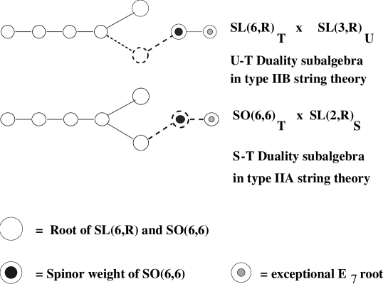
Figure 1:

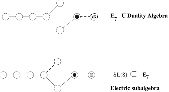
Figure 2:

From these embeddings occurring at the $E_{7}$ level, namely in $D=4$, one deduces the three embedding chains (28),(30),(31): it just suffices to peal off the last $\alpha_{r+1}$ roots one by one and also the $\beta$ root that occurs only in $D=4$. One observes that the appearance of the $\beta$ root is always responsible for an enhancement of the S–duality group. In the type IIA case this group is enhanced from $O(1,1)$ to $SL(2,{\rm I\kern-1.79993ptR})$ while in the type IIB case it is enhanced from the $SL(2,{\rm I\kern-1.79993ptR})_{U}$ already existing in $10$–dimensions to $SL(3,{\rm I\kern-1.79993ptR})$. Physically this occurs by combining the original dilaton field with the compactification radius of the latest compactified dimension.

4.2 String theory interpretation of the sequential embeddings: Type $IIA$, type $IIB$ and $M$ theory chains

We now turn to a closer analysis of the physical meaning of the embedding chains we have been illustrating.

Let us begin with the chain of eq.((30))that, as anticipated, is related with the type IIB interpretation of supergravity theory. The distinctive feature of this chain of embeddings is the presence of an addend $A_{1}$ that is already present in 10 dimensions. Indeed this $A_{1}$ is the Lie algebra of the $SL(2,R)_{\Sigma}$ symmetry of type $IIB$ D=10 superstring. We can name this group the U–duality symmetry $U_{10}$ in $D=10$. We can use the chain (30) to trace it in lower dimensions. Thus let us consider the decomposition

$$E_{r+1(r+1)} \rightarrow N_{r}\otimes SL(2,{\rm I\kern-1.79993ptR})$$

$$N_{r} = A_{r-1}\otimes O(1,1)$$ (35)

Obviously $N_{r}$ is not contained in the $T$-duality group $O(r,r)$ since the $NS$ tensor field $B_{\mu\nu}$ (which mixes with the metric under $T$-duality) and the $RR$–field $B^{c}_{\mu\nu}$ form a doublet with respect $SL(2,{\rm I\kern-1.79993ptR})_{U}$. In fact, $SL(2,{\rm I\kern-1.79993ptR})_{U}$ and $O(r,r)$ generate the whole U–duality group $E_{r+1(r+1)}$. The appropriate interpretation of the normaliser of $SL(2,R)_{\Sigma}$ in $E_{r+1(r+1)}$ is

$$N_{r}=O(1,1)\otimes SL(r,{\rm I\kern-1.79993ptR})\equiv GL(r,{\rm I\kern-1.79993ptR})$$ (36)

where $GL(r,{\rm I\kern-1.79993ptR})$ is the isometry group of the classical moduli space for the $T_{r}$ torus:

$$\frac{GL(r,{\rm I\kern-1.79993ptR})}{O(r)}.$$ (37)

The decomposition of the U–duality group appropriate for the type $IIB$ theory is

$$E_{r+1}\rightarrow U_{10}\otimes GL(r,{\rm I\kern-1.79993ptR})=SL(2,{\rm I\kern-1.79993ptR})_{U}\otimes O(1,1)\otimes SL(r,{\rm I\kern-1.79993ptR}).$$ (38)

Note that since $GL(r,{\rm I\kern-1.79993ptR})\supset O(1,1)^{r}$, this translates into $E_{r+1}\supset SL(2,{\rm I\kern-1.79993ptR})_{U}\otimes O(1,1)^{r}$. (In Type $IIA$, the corresponding chain would be $E_{r+1}\supset O(1,1)\otimes O(r,r)\supset O(1,1)^{r+1}$.) Note that while $SL(2,{\rm I\kern-1.79993ptR})$ mixes $RR$ and $NS$ states, $GL(r,{\rm I\kern-1.79993ptR})$ does not. Hence we can write the following decomposition for the solvable Lie algebra:

$$Solv\left(\frac{E_{r+1}}{H_{r+1}}\right) = Solv\left(\frac{GL(r,{\rm I\kern-1.79993ptR})}{O(r)}\otimes\frac{SL(2,{\rm I\kern-1.79993ptR})}{O(2)}\right)+\left(\frac{\bf r(r-1)}{\bf 2},{\bf 2}\right)\oplus{\bf X}\oplus{\bf Y}$$

$$\mbox{dim }Solv\left(\frac{E_{r+1}}{H_{r+1}}\right) = \frac{d(3d-1)}{2}+2+x+y.$$ (39)

where $x=\mbox{dim }{\bf X}$ counts the scalars coming from the internal part of the $4$–form $A^{+}_{{\mu}{\nu}{\rho}{\sigma}}$ of type IIB string theory. We have:

$$x=\left\{\matrix{0&r<4\cr\frac{r!}{4!(r-4)!}&r\geq 4\cr}\right.$$ (40)

and

$$y=\mbox{dim }{\bf Y}=\cases{\matrix{0&r<6\cr 2&r=6\cr}\cr}.$$ (41)

counts the scalars arising from dualising the two-index tensor fields in $r=6$.

For example, consider the $D=6$ case. Here the type $IIB$ decomposition is:

$$E_{5(5)}=\frac{O(5,5)}{O(5)\otimes O(5)}\rightarrow\frac{GL(4,{\rm I\kern-1.79993ptR})}{O(4)}\otimes\frac{SL(2,{\rm I\kern-1.79993ptR})}{O(2)}$$ (42)

whose compact counterpart is given by $O(10)\rightarrow SU(4)\otimes SU(2)\otimes U(1)$, corresponding to the decomposition: ${\bf 45}={\bf(15,1,1)}+{\bf(1,3,1)}+{\bf(1,1,1)}+{\bf(6,2,2)}+{\bf(1,1,2)}$. It follows:

$$Solv(\frac{E_{5(5)}}{O(5)\otimes O(5)})=Solv(\frac{GL(4,{\rm I\kern-1.79993ptR})}{O(4)}\otimes\frac{SL(2,{\rm I\kern-1.79993ptR})}{O(2)})+({\bf 6},{\bf 2})^{+}+({\bf 1},{\bf 1})^{+}.$$ (43)

where the factors on the right hand side parametrize the internal part of the metric $g_{ij}$, the dilaton and the $RR$ scalar ($\phi$, $\phi^{c}$), ($B_{ij}$, $B^{c}_{ij}$) and $A^{+}_{ijkl}$ respectively.

There is a connection between the decomposition ((35)) and the corresponding chains in M–theory. The type IIB chain is given by eq.((30)), namely by

$$E_{r+1(r+1)}\rightarrow SL(2,{\rm I\kern-1.79993ptR})\otimes GL(r,{\rm I\kern-1.79993ptR})$$ (44)

while the $M$ theory is given by eq.((31)), namely by

$$E_{r+1}\rightarrow O(1,1)\otimes SL(r+1,{\rm I\kern-1.79993ptR})$$ (45)

coming from the moduli space of $T^{11-D}=T^{r+1}$. We see that these decompositions involve the classical moduli spaces of $T^{r}$ and of $T^{r+1}$ respectively. Type $IIB$ and $M$ theory decompositions become identical if we decompose further $SL(r,{\rm I\kern-1.79993ptR})\rightarrow O(1,1)\times SL(r-1,{\rm I\kern-1.79993ptR})$ on the type $IIB$ side and $SL(r+1,{\rm I\kern-1.79993ptR})\rightarrow O(1,1)\otimes SL(2,{\rm I\kern-1.79993ptR})\otimes SL(r-1,{\rm I\kern-1.79993ptR})$ on the $M$-theory side. Then we obtain for both theories

$$E_{r+1}\rightarrow SL(2,{\rm I\kern-1.79993ptR})\times O(1,1)\otimes O(1,1)\otimes SL(r-1,{\rm I\kern-1.79993ptR}),$$ (46)

and we see that the group $SL(2,{\rm I\kern-1.79993ptR})_{U}$ of type $IIB$ is identified with the complex structure of the $2$-torus factor of the total compactification torus $T^{11-D}\rightarrow T^{2}\otimes T^{9-D}$.

Note that according to (34) in 8 and 4 dimensions, ($r=2$ and $6$) in the decomposition (46) there is the following enhancement:

$$SL(2,{\rm I\kern-1.79993ptR})\times O(1,1)\rightarrow SL(3,{\rm I\kern-1.79993ptR})\quad(\mbox{for}\,r=2,6)$$ (47)

$$\left\{\matrix{O(1,1)&\rightarrow&SL(2,{\rm I\kern-1.79993ptR})\quad(\mbox{for}\,r=2)\cr SL(5,{\rm I\kern-1.79993ptR})\times O(1,1)&\rightarrow&SL(6,{\rm I\kern-1.79993ptR})\quad(\mbox{for}\,r=6)\cr}\right.$$ (48)

Finally, by looking at fig.(3) let us observe that $E_{7(7)}$ admits also a subgroup $SL(2,{\rm I\kern-1.79993ptR})_{T}$ $\otimes(SO(5,5)_{S}$ $\equiv E_{5(5)})$ where the $SL(2,{\rm I\kern-1.79993ptR})$ factor is a T–duality group, while the factor $(SO(5,5)_{S}$ $\equiv E_{5(5)})$ is an S–duality group which mixes RR and NS states.

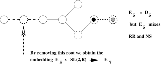
Figure 3:

5 The maximal abelian ideals ${\cal A}_{r+1}\subset Solv_{r+1}$ of the solvable Lie algebra

It is interesting to work out the maximal abelian ideals ${\cal A}_{r+1}\subset Solv_{r+1}$ of the solvable Lie algebras generating the scalar manifolds of maximal supergravity in dimension $D=10-r$. The maximal abelian ideal of a solvable Lie algebra is defined as the maximal subset of nilpotent generators commuting among themselves. From a physical point of view this is the largest abelian Lie algebra that one might expect to be able to gauge in the supergravity theory. Indeed, as it turns out, the number of vector fields in the theory is always larger or equal than $\mbox{dim}{\cal A}_{r+1}$. Actually, as we are going to see, the gaugeable maximal abelian algebra is always a proper subalgebra ${\cal A}^{gauge}_{r+1}\subset{\cal A}_{r+1}$ of this ideal.

The criteria to determine ${\cal A}^{gauge}_{r+1}$ will be discussed in the next section. In the present section we derive ${\cal A}_{r+1}$ and we explore its relation with the space of vector fields in one dimension above the dimension we each time consider. From such analysis we obtain a filtration of the solvable Lie algebra which provides us with a canonical polynomial parametrization of the supergravity scalar coset manifold $U_{r+1}/H_{r+1}$

5.1 The maximal abelian ideal from an algebraic viewpoint

Algebraically the maximal abelian ideal can be characterized by looking at the decomposition of the U–duality algebra $E_{r+1(r+1)}$ with respect to the U–duality algebra in one dimension above. In other words we have to consider the decomposition of $E_{r+1(r+1)}$ with respect to the subalgebra $E_{r(r)}\,\otimes\,O(1,1)$. This decomposition follows a general pattern which is given by the next formula:

$$\mbox{adj }E_{r+1(r+1)}\,=\,\mbox{adj }E_{r(r)}\,\oplus\,\mbox{adj }O(1,1)\,\oplus({\rm I\kern-1.79993ptD}^{+}_{r}\oplus{\rm I\kern-1.79993ptD}^{-}_{r})$$ (49)

where ${\rm I\kern-1.79993ptD}^{+}_{r}$ is at the same time an irreducible representation of the U–duality algebra $E_{r(r)}$ in $D+1$ dimensions and coincides with the maximal abelian ideal

$${\rm I\kern-1.79993ptD}^{+}_{r}\,\equiv\,{\cal A}_{r+1}\,\subset\,Solv_{(r+1)}$$ (50)

of the solvable Lie algebra we are looking for. In eq. (49) the subspace ${\rm I\kern-1.79993ptD}^{-}_{r}$ is just a second identical copy of the representation ${\rm I\kern-1.79993ptD}^{+}_{r}$ and it is made of negative rather than of positive weights of $E_{r(r)}$. Furthermore ${\rm I\kern-1.79993ptD}^{+}_{r}$ and ${\rm I\kern-1.79993ptD}^{-}_{r}$ correspond to the eigenspaces belonging respectively to the eigenvalues $\pm 1$ with respect to the adjoint action of the S–duality group $O(1,1)$.

5.2 The maximal abelian ideal from a physical perspective: the vector fields in one dimension above and translational symmetries

Here, we would like to show that the dimension of the abelian ideal in $D$ dimensions is equal to the number of vectors in dimensions $D+1$. Denoting the number of compactified dimensions by $r$ (in string theory, $r=10-D$), we will label the $U$-duality group in $D$ dimensions by $U_{D}=E_{11-D}=E_{r+1}$. The $T$-duality group is $O(r,r)$, while the $S$-duality group is $O(1,1)$ in dimensions higher than four, $SL(2,R)$ in $D=4$ (and it is inside $O(8,8)$ in $D=3$).

It follows from (49) that the total dimension of the abelian ideal is given by

$${\rm dim}\,{\cal A}_{D}\,\equiv\,{\rm dim}\,{\cal A}_{r+1}\,\equiv\,{\rm dim}\,{\rm I\kern-1.79993ptD}_{r}$$ (51)

where ${\rm I\kern-1.79993ptD}_{r}$ is a representation of $U_{D+1}$ pertaining to the vector fields. According to (49) we have (for $D\geq 4$):

$$\mbox{adj }U_{D}=\mbox{adj }U_{D+1}\oplus{\bf 1}\oplus({\bf 2},{\rm I\kern-1.79993ptD}_{r}).$$ (52)

This is just an immediate consequence of the embedding chain (27) which at the first level of iteration yields $E_{r+1}\rightarrow E_{r}\times O(1,1)$. For example, under $E_{7}\rightarrow E_{6}\times O(1,1)$ we have the branching rule: ${\rm adj}\,E_{7}={\rm adj}\,E_{6}+{\bf 1}+({\bf 2},{\bf 27})$ and the abelian ideal is given by the ${\bf 27^{+}}$ representation of the $E_{6(6)}$ group. The $70$ scalars of the $D=4,N=8$ theory are naturally decomposed as ${\bf 70}={\bf 42}+{\bf 1}+{\bf 27^{+}}$. To see the splitting of the abelian ideal scalars into $NS$ and $RR$ sectors, one has to consider the decomposition of $U_{D+1}$ under the T–duality group $T_{D+1}=O(r-1,r-1)$, namely the second iteration of the embedding chain (27): $E_{r+1}\rightarrow O(1,1)\times O(r-1,r-1)$. Then the vector representation of $O(r-1,r-1)$ gives the $NS$ sector, while the spinor representation yields the $RR$ sector. The example of $E_{7}$ considered above is somewhat exceptional, since we have ${\bf 27}\rightarrow({\bf 10}+{\bf 1}+{\bf 16})$. Here in addition to the expected ${\bf 10}$ and ${\bf 16}$ of $O(5,5)$ we find an extra $NS$ scalar: physically this is due to the fact that in four dimensions the two-index antisymmetric tensor field $B_{\mu\nu}$ is dual to a scalar, algebraically this generator is associated with the exceptional root $\sqrt{2}\epsilon_{7}$. To summarize, the $NS$ and $RR$ sectors are separately invariant under $O(r,r)$ in $D=10-r$ dimensions, while the abelian $NS$ and $RR$ sectors are invariant under $O(r-1,r-1)$. The standard parametrization of the $U_{D}/H_{D}$ and $U_{D+1}/H_{D+1}$ cosets gives a clear illustration of this fact:

$$\frac{U_{D}}{H_{D}}\sim(\frac{U_{D+1}}{H_{D+1}},r_{D+1},{\bf V}_{r}^{D+1}).$$ (53)

Here $r_{D+1}$ stands for the compactification radius, and ${\bf V}_{r}^{D+1}$ are the compactified vectors yielding the abelian ideal in $D$ dimensions.

Note that:

$$\mbox{adj}\,H_{D}=\mbox{adj}\,H_{D+1}\,+\,\mbox{adj}\,\mbox{Irrep}\,U_{D+1}$$ (54)

so it appears that the abelian ideal forms a representation not only of $U_{D+1}$ but also of the compact isotropy subgroup $H_{D+1}$ of the scalar coset manifold.

In the above $r=6$ example we find ${\rm adj}\,SU(8)={\rm adj}\,USp(8)\oplus{\bf 27^{-}}$, $\Longrightarrow$ ${\bf 63}={\bf 36}+{\bf 27^{-}}$.

6 Gauging

In this last section we will consider the problem of gauging some isometries of the coset $G/H$ in the framework of solvable Lie algebras.

In particular we will consider in more detail the gauging of maximal compact groups and the gauging of nilpotent abelian (translational) isometries.

This procedure is a way of obtaining partial supersymmetry breaking in extended supergravities [33],[35],[36] and it may find applications in the context of non perturbative phenomena in string and M-theories.

Let us consider the left–invariant 1–form $\Omega=L^{-1}dL$ of the coset manifold $U_{D}/H_{D}$, where $L$ is the coset representative.

The gauging procedure [37] amounts to the replacement of $dL$ with the gauge covariant differential $\nabla L$ in the definition of the left–invariant 1–form $\Omega=L^{-1}dL$:

$$\Omega\rightarrow\widehat{\Omega}=L^{-1}\nabla L=L^{-1}(d+A)L=\Omega+L^{-1}AL$$ (55)

As a consequence $\widehat{\Omega}$ is no more a flat connection, but its curvature is given by:

$$R(\widehat{\Omega})=d\widehat{\Omega}+\widehat{\Omega}\wedge\widehat{\Omega}=L^{-1}{\cal F}L\equiv L^{-1}(dA+A\wedge A)L=L^{-1}(F^{I}T_{I}+L^{I}_{AB}T_{I}\overline{\psi}^{A}\psi^{B})L$$ (56)

where $F^{I}$ is the gauged supercovariant 2–form and $T_{I}$ are the generators of the gauge group embedded in the U–duality representation of the vector fields.

Indeed, by very definition, under the full group $E_{r+1(r+1)}$ the gauge vectors are contained in the representation ${\rm I\kern-1.79993ptD}_{r+1}$. Yet, with respect to the gauge subgroup they must transform in the adjoint representation, so that ${\cal G}_{D}$ has to be chosen in such a way that:

$${\rm I\kern-1.79993ptD}_{r+1}\,\stackrel{{\scriptstyle{\cal G}_{D}}}{{\longrightarrow}}\,\mbox{adj}\,{\cal G}_{D}\,\oplus\,\mbox{rep}\,{\cal G}_{D}$$ (57)

where $\mbox{rep}\,{\cal G}_{D}$ is some other representation of ${\cal G}_{D}$ contained in the above decomposition.

It is important to remark that vectors which are in $\mbox{rep}{\cal G}_{D}$ (i.e. vectors which do not gauge ${\cal G}_{D}$) may be required, by consistence of the theory [38], to appear through their duals $(D-3)$–forms, as for instance happens for $D=5$ [39]. In an analogous way $p$–form potentials ($p\neq 1$) which are in non trivial representations of ${\cal G}_{D}$ may also be required to appear through their duals $(D-p-2)$–potentials, as is the case in $D=7$ for $p=2$ [40].

The charges and the boosted structure constants discussed in the next subsection can be retrieved from the two terms appearing in the last expression of eq. (56)

6.1 Filtration of the $E_{r+1}$ root space, canonical parametrization of the coset representatives and boosted structure constants

As it has already been emphasized in the introduction, the complete structure of $N>2$ supergravity in diverse dimensions is fully encoded in the local differential geometry of the scalar coset manifold $U_{D}/H_{D}$. All the couplings in the Lagrangian are described in terms of the metric, the connection and the coset representative (11) of $U_{D}/H_{D}$. A particularly significant consequence of extended supersymmetry is that the fermion masses and the scalar potential the theory can develop occur only as a consequence of the gauging and can be extracted from a decomposition in terms of irreducible $H_{D}$ representations of the boosted structure constants[41] [37]. Let us define these latter. Let ${\rm I\kern-1.79993ptD}_{r+1}$ be the irreducible representation of the $U_{D}$ U–duality group pertaining to the vector fields and denote by ${\vec{\bf w}}_{\Lambda}$ a basis for ${\rm I\kern-1.79993ptD}_{r+1}$:

$$\forall{\vec{\bf v}}\,\in\,{\rm I\kern-1.79993ptD}_{r+1}\qquad:\qquad{\vec{v}}\,=\,v^{\Lambda}\,{\vec{\bf w}}_{\Lambda}$$ (58)

In the case we consider of maximal supergravity theories, where the U–duality groups are given by $E_{r+1(r+1)}$ the basis vectors ${\vec{\bf w}}_{\Lambda}$ can be identified with the $56$ weights of the fundamental $E_{7(7)}$ representation or with the subsets of this latter corresponding to the irreducible representations of its $E_{r+1(r+1)}$ subgroups, according to the branching rules:

$${\bf 56}{\stackrel{{\scriptstyle E_{6}}}{{\longrightarrow}}}\cases{{\bf 27+1}{\stackrel{{\scriptstyle E_{5}}}{{\longrightarrow}}}\cases{{\bf 16}{\stackrel{{\scriptstyle E_{4}}}{{\longrightarrow}}}{\bf\dots}\cr{\bf 10}{\stackrel{{\scriptstyle E_{4}}}{{\longrightarrow}}}{\bf\dots}\cr{\bf 1+1}{\stackrel{{\scriptstyle E_{4}}}{{\longrightarrow}}}{\bf\dots}\cr}\cr{\bf 27+1}{\stackrel{{\scriptstyle E_{5}}}{{\longrightarrow}}}\cases{{\bf 16}{\stackrel{{\scriptstyle E_{4}}}{{\longrightarrow}}}{\bf\dots}\cr{\bf 10}{\stackrel{{\scriptstyle E_{4}}}{{\longrightarrow}}}{\bf\dots}\cr{\bf 1+1}{\stackrel{{\scriptstyle E_{4}}}{{\longrightarrow}}}{\bf\dots}\cr}\cr}$$ (59)

Let:

$$<~{},~{}>\quad:\quad{\rm I\kern-1.79993ptD}_{r+1}\,\times{\rm I\kern-1.79993ptD}_{r+1}\,\longrightarrow\,{\rm I\kern-1.79993ptR}$$ (60)

denote the invariant scalar product in ${\rm I\kern-1.79993ptD}_{r+1}$ and let ${\vec{\bf w}}^{\Sigma}$ be a dual basis such that

$$<{\vec{\bf w}}^{\Sigma},{\vec{\bf w}}_{\Lambda}>\,=\,\delta^{\Sigma}_{\Lambda}$$ (61)

Consider then the ${\rm I\kern-1.79993ptD}_{r+1}$ representation of the coset representative (11):

$$L(\phi)\quad:\quad|{\vec{\bf w}}_{\Lambda}>\,\longrightarrow L(\phi)_{\Lambda}^{\Sigma}\,|{\vec{\bf w}}_{\Sigma}>,$$ (62)

and let $T^{I}$ be the generators of the gauge algebra ${\cal G}_{D}\,\subset E_{r+1(r+1)}$.

The only admitted generators are those with index $\Lambda=I\,\in\,{adj}\,{\cal G}_{D}$, and there are no gauge group generators with index $\Lambda\,\in\,\mbox{rep}\,{\cal G}_{D}$. Given these definitions the boosted structure constants are the following three–linear $3$–tensors in the coset representatives:

$$\,\hbox{$\vrule height=6.45831pt,width=0.4pt,depth=0.0pt\kern-3.00003pt{\rm C}$}_{\Sigma\Gamma}^{\Lambda}\left(\phi\right)\,\equiv\,\sum_{I=1}^{{\rm dim}{\cal G}_{D}}\,<{\vec{\bf w}}^{\Lambda}\,,\,L^{-1}\left(\phi\right)\,T_{I}\,L\left(\phi\right)\,{\vec{\bf w}}_{\Sigma}>\,<{\vec{\bf w}}^{I}\,,\,L\left(\phi\right){\vec{\bf w}}_{\Gamma}>$$ (63)

and by decomposing them into irreducible $H_{r+1}$ representations we obtain the building blocks utilized by supergravity in the fermion shifts, in the fermion mass–matrices and in the scalar potential.

In an analogous way, the charges appearing in the gauged covariant derivatives are given by the following general form:

$$Q_{I\Sigma}^{\Lambda}\,\equiv\,<{\vec{\bf w}}^{\Lambda}\,,\,L^{-1}\left(\phi\right)\,T_{I}\,L\left(\phi\right)\,{\vec{\bf w}}_{\Sigma}>$$ (64)

The coset representative $L\left(\phi\right)$ can be written in a canonical polynomial parametrization which should give a simplifying tool in mastering the scalar field dependence of all physical relevant quantities. This includes, besides mass matrices, fermion shifts and scalar potential, also the central charges [42].

The alluded parametrization is precisely what the solvable Lie algebra analysis produces.

To this effect let us decompose the solvable Lie algebra of $E_{7(7)}/SU(8)$ in a sequential way utilizing eq. (49). Indeed we can write the equation:

$$Solv(E_{7(7)})={\cal H}_{7}\oplus\Phi^{+}(E_{7})$$ (65)

where $\Phi^{+}(E_{7})$ is the $63$ dimensional positive part of the $E_{7}$ root space. By repeatedly using eq. (49) we obtain:

$$\Phi^{+}(E_{7})=\Phi^{+}(E_{2})\oplus{\rm I\kern-1.79993ptD}^{+}_{2}\oplus{\rm I\kern-1.79993ptD}^{+}_{3}\oplus{\rm I\kern-1.79993ptD}^{+}_{4}\oplus{\rm I\kern-1.79993ptD}^{+}_{5}\oplus{\rm I\kern-1.79993ptD}^{+}_{6}$$ (66)

where $\Phi^{+}(E_{2})$ is the one–dimensional root space of the U–duality group in $D=9$ and ${\rm I\kern-1.79993ptD}^{+}_{r+1}$ are the weight-spaces of the $E_{r+1}$ irreducible representations to which the vector field in $D=10-r$ are assigned. Alternatively, as we have already explained, ${\cal A}_{r+2}\equiv{\rm I\kern-1.79993ptD}^{+}_{r+1}$ are the maximal abelian ideals of the U–duality group in $E_{r+2}$ in $D=10-r-1$ dimensions.

We can easily check that the dimensions sum appropriately as follows from:

$$\mbox{dim}\,\Phi^{+}(E_{7})\, = {63}$$

$$\mbox{dim}\,\Phi^{+}(E_{2})\, = {1}\quad\quad~{}\mbox{dim}\,{\rm I\kern-1.79993ptD}^{+}_{2}\,={3}$$

$$\mbox{dim}\,{\rm I\kern-1.79993ptD}^{+}_{3}\, = {6}\quad\quad~{}\mbox{dim}\,{\rm I\kern-1.79993ptD}^{+}_{4}\,={10}$$

$$\mbox{dim}\,{\rm I\kern-1.79993ptD}^{+}_{5}\, = {16}\quad\quad\mbox{dim}\,{\rm I\kern-1.79993ptD}^{+}_{4}\,={27}$$

Relying on eq. (65), (66) we can introduce a canonical set of scalar field variables:

$$\phi^{i} \longrightarrow Y_{i}\,\in{\cal H}\quad\quad i=1,\dots\,r$$

$$\tau^{i}_{k} \longrightarrow \,D^{(k)}_{i}\,\in{\rm I\kern-1.79993ptD}_{k}\quad i=1,\dots\,\mbox{dim }\,{\rm I\kern-1.79993ptD}_{k}\quad(k=2,\dots,6)$$

$$\tau_{1} \longrightarrow {\rm I\kern-1.79993ptD}_{1}\,\equiv\,E_{2}$$ (68)

and adopting the short hand notation:

$$\phi\cdot{\cal H} \equiv \phi^{i}\,Y_{i}$$

$$\tau_{k}\cdot{\rm I\kern-1.79993ptD}_{k} \equiv \tau^{i}_{k}\,D^{(k)}_{i}$$

we can write the coset representative for maximal supergravity in dimension $D=10-r$ as:

$$L = \exp\left[\phi\cdot{\cal H}\right]\,\prod_{k=1}^{r}\,\exp\left[\tau_{k}\cdot{\rm I\kern-1.79993ptD}_{k}\right]$$ (70)

The relevant point is that, defining:

$$S^{i}\,\equiv\,\exp[\phi^{i}Y_{i}]$$ (71)

all entries of the matrix $L$ are polynomials in the $S^{i},\tau^{i}_{k},\tau_{1}$ “canonical” variables. This follows from the fact that all the matrices $\tau_{k}\cdot{\rm I\kern-1.79993ptD}_{k}$ are nilpotent (at most of order 4). Furthermore when the gauge group is chosen within the maximal abelian ideal it is evident from the definition of the boosted structure constants (63) that they do not depend on the scalar fields associated with the generators of the same ideal. In such gauging one has therefore a flat direction of the scalar potential for each generator of the maximal abelian ideal.

In the next section we turn to considering the possible gaugings more closely.

6.2 Gauging of compact and translational isometries

A necessary condition for the gauging of a subgroup ${\cal G}_{D}\subset U_{D}$ is that the representation of the vectors ${\rm I\kern-1.79993ptD}_{r+1}$ must contain $\mbox{adj}{\cal G}_{D}$. Following this prescription, the list of maximal compact gaugings ${\cal G}_{D}$ in any dimensions is obtained in the third column of Table 4. In the other columns we list the $U_{D}$-duality groups, their maximal compact subgroups and the left-over representations for vector fields.

Table 4: Maximal gauged compact groups

$D$	$U_{D}$	$H_{D}$	${\cal G}_{D}$	$\mbox{rep}{\cal G}_{D}$
9	$SL(2,{\rm I\kern-1.79993ptR})\times O(1,1)$	$O(2)$	$O(2)$	2
8	$SL(3,{\rm I\kern-1.79993ptR})\times SL(2,{\rm I\kern-1.79993ptR})$	$O(3)\times O(2)$	$O(3)$	$3$
7	$SL(5,{\rm I\kern-1.79993ptR})$	$USp(4)$	$O(5)\sim USp(4)$	0
6	$O(5,5)$	$USp(4)\times USp(4)$	$O(5)$	$5+1$
5	$E_{6,(6)}$	$USp(8)$	$O(6)\sim SU(4)$	$2\times 6$
4	$E_{7(7)}$	$SU(8)$	$O(8)$	0

Table 5: Transformation properties under ${\cal G}_{D}$ of 2- and 3-forms

$D$	$\mbox{rep}\,B_{\mu\nu}$	$\mbox{rep}\,A_{\mu\nu\rho}$
9	2	0
8	3	0
7	0	5
6	5	0
5	$2\times 6$	0

We notice that, for any $D$, there are $p$–forms ($p$ =1,2,3) which are charged under the gauge group ${\cal G}_{D}$. Consistency of these theories requires that such forms become massive. It is worthwhile to mention how this can occur in two variants of the Higgs mechanism. Let us define the (generalized) Higgs mechanism for a $p$–form mass generation through the absorption of a massless ($p-1$)–form (for $p=1$ this is the usual Higgs mechanism). The first variant is the anti-Higgs mechanism for a $p$–form [43], which is its absorption by a massless ($p+1$)–form. It is operating, for $p=1$, in $D=5,6,8,9$ for a sextet of $SU(4)$, a quintet of $SO(5)$, a triplet of $SO(3)$ and a doublet of $SO(2)$, respectively. The second variant is the self–Higgs mechanism [38], which only exists for $p=(D-1)/2$, $D=4k-1$. This is a massless $p$–form which acquires a mass through a topological mass term and therefore it becomes a massive “chiral” $p$–form. The latter phenomena was shown to occur in $D=3$ and $7$. It is amazing to notice that the representation assignments dictated by $U$–duality for the various $p$–forms is precisely that needed for consistency of the gauging procedure (see Table 5).

The other compact gaugings listed in Table 4 are the $D=4$ [44] and $D=8$ cases [45].

It is possible to extend the analysis of gauging semisimple groups also to the case of solvable Lie groups [46]. For the maximal abelian ideals of $Solv(U_{D}/H_{D})$ this amounts to gauge an $n$–dimensional subgroup of the translational symmetries under which at least $n$ vectors are inert. Indeed the vectors the set of vectors that can gauge an abelian algebra (being in its adjoint representation) must be neutral under the action of such an algebra. We find that in any dimension $D$ the dimension of this abelian group $\mbox{dim}{\cal G}_{abel}$ is given precisely by ${\rm dim}(\mbox{rep}{\cal G}_{D})$ which appear in the decomposition of ${\rm I\kern-1.79993ptD}_{r+1}$ under $O(r+1)$. We must stress that this criterium gives a necessary but not sufficient condition for the existence of the gauging of an abelian isometry group, consistent with supersymmetry.

Table 6: Decomposition of fields in representations of the compact group ${\cal G}_{D}=O(11-D)$

	vect. irrep	adj($O(11-D)$)	${\cal A}$	$\mbox{dim}{\cal G}_{abel}$
$D=9$	$1+2$	1	1	1
$D=8$	$3+3$	3	3	3
$D=7$	$6+4$	6	6	4
$D=6$	$10+5+1$	10	10	$5+1$
$D=5$	$15+6+6$	15	$15+1$	$6+6$
$D=4$	$(21+7)\times 2$	21	$21+1\times 6$	7

As already remarked in the introduction it is reasonable to expect that the gauging of translational isometries and its consequence, namely the spontaneous breaking of supersymmetry, should be generated in the effective quantum lagrangian by the condensation of field strengths. This will occur through the summation on non perturbative states, namely on BPS monopoles, black-holes and $p$-branes.

Hence, in the next section, I turn to discuss these topics.

7 BPS States in rigid N=2 supersymmetry

The most general form of a rigid N=2 super Yang–Mills Lagrangian was derived in [8]: its structure is fully determined by three geometrical data:

• The choice of a Special Kähler manifold of the rigid type ${\cal SK}^{rig}$ describing the vector multiplet couplings

• The choice of a HyperKähler manifold ${\cal HK}$ describing the hypermultiplet dynamics

• The choice of a gauge group $G^{gauge}\subset G^{iso}$, subgroup of the isometry group of both ${\cal SK}^{rig}$ and ${\cal HK}$

The bosonic action has the following form:

$${\cal L}_{N=2\,SUSY}^{Bose} = g_{i{{j}^{\star}}}\,\nabla^{\mu}z^{i}\nabla_{\mu}\overline{z}^{{j}^{\star}}\,+\,h_{uv}\,\nabla_{\mu}\,q^{u}\,\nabla^{\mu}\,q^{v}-\,{\rm V}\bigl{(}z,{\overline{z}},q\bigr{)}$$ (72)

$$+\,{\rm i}\,\left(\overline{\cal N}_{IJ}{\cal F}^{-I}_{\mu\nu}{\cal F}^{-J|{\mu\nu}}\,-\,{\cal N}_{IJ}{\cal F}^{+I}_{\mu\nu}{\cal F}^{+J|{\mu\nu}}\right)$$

where the scalar potential is expressed in terms of the killing vectors $k^{i}_{I}$, $k^{u}_{I}$ generating the gauge group algebra on the scalar manifold ${\cal SK}\otimes{\cal HQ}$, of the upper half $Y^{J}(z)$ of the symplectic section of rigid special geometry and also in terms of the momentum map functions ${\cal P}^{x}_{I}(q)$ yielding the Poissonian realization of the gauge group algebra on the HyperKähler manifold:

$$\,-{\rm V}\bigl{(}z,{\overline{z}},q\bigr{)} = -\,g^{2}\,\Bigl{[}\left(g_{i{{j}^{\star}}}\,k^{i}_{I}\,k^{{j}^{\star}}_{J}+\,4\,h_{uv}k^{u}_{I}\,k^{v}_{J}\right)\,\overline{Y}^{I}\,Y^{J}+\,g^{i{{j}^{\star}}}\,f^{I}_{i}\,f^{J}_{{j}^{\star}}\,{\cal P}^{x}_{I}\,{\cal P}^{x}_{J}\,\Bigr{]}$$

The kinetic term of the vectors in (72) involves the period matrix ${\cal N}_{IJ}$, which is also a datum of rigid special geometry.

If we restrict our attention to a pure gauge theory without hypermultiplets, and we calculate the energy of a generic static configuration (i.e $F^{I}_{0a}$ = $0$, $\nabla_{0}z^{i}$ = $0$), we obtain:

$$E = \int\,d^{3}x\Bigl{[}\mbox{Im}{\cal N}_{IJ}F^{I}_{ab}\,F^{J}_{ab}+\,g_{i{{j}^{\star}}}\,\nabla_{a}z^{i}\,\nabla_{a}{\overline{z}}^{j^{\star}}\,+\,g^{2}\,g_{i{{j}^{\star}}}\,k^{i}_{I}\,k^{{j}^{\star}}_{J}\,\overline{Y}^{I}\,Y^{J}\Bigr{]}$$

Using the special geometry identity:

$$U^{IJ}\equiv g^{i{{j}^{\star}}}\,{\overline{f}}^{J}_{j^{\star}}\,f^{I}_{i}\,=\,-\,\frac{1}{2}\,\left(\mbox{Im}{\cal N}\right)^{-1|IJ}$$ (75)

the energy integral (LABEL:monenergy) can be rewritten according to a Bogomolny decomposition as follows:

$$E = \int\,d^{3}x\,\frac{1}{2}\,g_{i{{j}^{\star}}}\left(2\mbox{i}\,G^{i}_{ab}\pm\epsilon_{abc}\nabla_{c}z^{i}\right)\,\left(-2\mbox{i}\,G^{j^{\star}}_{ab}\pm\epsilon_{abc}\nabla_{c}z^{j^{\star}}\right)$$ (78)

$$+\int\,d^{3}x\,\,g^{2}\,g_{i{{j}^{\star}}}\,k^{i}_{I}\,k^{{j}^{\star}}_{J}\,\overline{Y}^{I}\,Y^{J}$$

$$\pm\int\,d^{3}x\,\mbox{i}\epsilon_{abc}\left(G^{j^{\star}}_{ab}\nabla_{c}z^{i}\,-\,G^{i}_{ab}\nabla_{c}z^{j^{\star}}\right)$$

where, by definition:

$$G^{i}_{\mu\nu}\,\equiv\,g^{i{{j}^{\star}}}\,{\overline{f}}^{I}_{j^{\star}}\,\mbox{Im}{\cal N}_{IJ}F^{J}_{\mu\nu}\quad;\quad{\overline{f}}^{I}_{j^{\star}}\equiv\nabla_{j^{\star}}{\overline{Y}}^{I}$$ (79)

The last (78) of the three addends contributing to the energy is the integral of a total divergence and can be identified with the topological charge of the configuration:

$$Z\,\equiv\,2\int_{S_{\infty}^{2}}\,\mbox{Im}{\cal N}_{IJ}F^{I}\,\mbox{Im}Y^{J}$$

$$=2\int_{R^{3}}\,\mbox{Im}{\cal N}_{IJ}F^{I}\,\wedge\nabla\mbox{Im}Y^{J}$$

$$=\int\,d^{3}x\,\mbox{i}\epsilon_{abc}\left(G^{j^{\star}}_{ab}\nabla_{c}z^{i}\,-\,G^{i}_{ab}\nabla_{c}z^{j^{\star}}\right)\,g_{ij^{\star}}$$ (80)

where $S_{\infty}^{2}$ is the $2$–sphere at infinity bounding a constant time slice of space–time. Since the other two addends (78),(78) to the energy of the static configuration are integrals of perfect squares, it follows that in each topological sector, namely at fixed value of the topological charge $Z$ the mass satisfies the Bogomolny bound (4). Furthermore a BPS saturated state (monopole or dyon) is defined by the two conditions:

$$2\mbox{i}\,G^{i}_{ab}\pm\epsilon_{abc}\nabla_{c}z^{i}=0$$ (81)

$$g^{2}\,g_{i{{j}^{\star}}}\,k^{i}_{I}\,k^{{j}^{\star}}_{J}\,\overline{Y}^{I}\,Y^{J}=0$$ (82)

The relation with the preservation of $\frac{1}{2}$ supersymmetries can now be easily seen. In a bosonic background the supersymmetry variation of the bosons is automatically zero since it is proportional to the fermion fields which are zero: one has just to check the supersymmetry variation of the fermion fields. In the theory under consideration the only fermionic field is the gaugino and its SUSY variation is given by (see [8]):

$$\delta\lambda^{iA} = \mbox{i}\nabla_{\mu}z^{i}\,\gamma^{\mu}\,\epsilon^{A}+\varepsilon^{AB}\left(G^{-i}_{\mu\nu}\,\gamma^{\mu\nu}+k^{i}_{I}{\overline{Y}}^{I}\right)\,\epsilon_{B}$$ (83)

If we use a SUSY parameter subject to the condition:

$$\gamma_{0}\,\epsilon^{A}\,=\,\pm\mbox{i}\,\varepsilon^{AB}\,\epsilon_{B}$$ (84)

then, in a static bosonic background eq.(83) becomes:

$$\delta\lambda^{iA} = \Bigl{[}-\mbox{i}\,\frac{1}{2}\,\left(2\mbox{i}\,G^{i}_{ab}\pm\epsilon_{abc}\,\nabla_{c}z^{i}\right)\,\gamma^{ab}\,\epsilon_{B}\,+k^{i}_{I}{\overline{Y}}^{I}\,\epsilon_{B}\,\Bigr{]}\,\varepsilon^{AB}\,$$ (85)

Henceforth the configuration is invariant under the supersymmetries of type (84) if and only if eq.(81) is satisfied together with:

$$k^{i}_{I}{\overline{Y}}^{I}\,=\,0$$ (86)

Eq.(86) is nothing else but the square–root of eq.(82). So we can conclude that the BPS saturated states are just those configurations which are invariant under supersymmetries of type (84). On the other hand, these supersymmetries are, by definition, those generated by the operators (5). So by essential use of the rigid special geometry structure we have shown the match between the abstract reasoning of section  2 and the concrete field theory realization of BPS saturated states.

8 BPS black holes in N=2 local supersymmetry

Eq.(84) is not Lorentz invariant and introduces a clear–cut separation between space and time. The interpretation of this fact is that we are dealing with localized lumps of energy that can be interpreted as quasi–particles at rest. A Lorentz boost simply puts such quasi–particles into motion. In the gravitational case the generalization of eq.(84) requires the existence of a time–like killing vector $\xi^{\mu}$, in order to write:

$$\xi^{\mu}\,\gamma_{\mu}\,\epsilon^{A}\,=\,\pm\mbox{i}\,\varepsilon^{AB}\,\epsilon_{B}$$ (87)

Furthermore, the analogue of the localization condition corresponds to the asymptotic flatness of space–time.

We are therefore led to look for the BPS saturated states of local $N=2$ supersymmetry within the class of electrically and magnetically charged, asymptotically flat, static space–times. Generically such space–times are black–holes since they have singularities hidden by horizons. Without the constraints imposed by supersymmetry the horizons can also disappear and there exist configurations that display naked singularities. In the supersymmetric case, however, the Bogomolny bound (4) becomes the statement that the ADM mass of the black–hole is always larger or equal than the central charge. This condition just ensures that the horizon exists. Hence the cosmic censorship conjecture is just a consequence of $N\geq 2$ supersymmetry. This was noted for the first time in [13]. The BPS saturated black–holes are configurations for which the horizon area is minimal at fixed electric and magnetic charges. This result was obtained by Ferrara and Kallosh in [16, 14].They are determined by solving the gravitational analogue of the Bogomolny first order equations (81), (86), obtained from the SUSY variation of the fermions.

If we restrict our attention to the gravitational coupling of vector multiplets, the bosonic action we have to consider is the following one:

$$S^{Bose}_{N=2} = \int\sqrt{-g}\,d^{4}\,x{\cal L}$$

$${\cal L} = -{1\over 2}\,R\,+\,g_{i{{j}^{\star}}}\,\nabla^{\mu}z^{i}\nabla_{\mu}\overline{z}^{{j}^{\star}}+\,{\rm i}\,\left(\overline{\cal N}_{\Lambda\Sigma}{\cal F}^{-\Lambda}_{\mu\nu}{\cal F}^{-\Sigma|{\mu\nu}}\,-\,{\cal N}_{\Lambda\Sigma}{\cal F}^{+\Lambda}_{\mu\nu}{\cal F}^{+\Sigma|{\mu\nu}}\right)$$ (88)

$$-\,g^{2}\,g_{i{{j}^{\star}}}\,k^{i}_{\Lambda}\,k^{{j}^{\star}}_{\Sigma}\,\overline{L}^{\Lambda}\,L^{\Sigma}$$

where $L^{\Lambda}$ denotes the upper half of a covariantly holomorphic section of local special geometry and ${\cal N}_{\Lambda\Sigma}$ is the period matrix according to its local rather than rigid definition (see [2],[8]). According to the previous discussion we consider for the metric an ansatz of the following form:

$$ds^{2}\,=\,e^{2U(r)}\,dt^{2}\,-\,e^{-2U(r)}d{\vec{x}}^{2}$$ (89)

where ${\vec{x}}$ are isotropic coordinates on ${\rm I\kern-1.79993ptR}^{3}$ and $U(r)$ is a function only of:

$$r\equiv\sqrt{{\vec{x}}^{2}}$$ (90)

As we shall see in the next section, eq.(89) corresponds to a 0–brane ansatz. This is in line with the fact that we have 1–form gauge fields in our theory that couple to 0–branes, namely to particle world–lines. Indeed, in order to proceed further we need an ansatz for the gauge field strengths. To this effect we begin by constructing a 2–form which is anti–self–dual in the background of the metric (89) and whose integral on the $2$–sphere at infinity $S^{2}_{\infty}$ is normalized to $2\pi$. A short calculation yields:

$$E^{-} = \mbox{i}\frac{e^{2U(r)}}{r^{3}}\,dt\wedge{\vec{x}}\cdot d{\vec{x}}+\frac{1}{2}\frac{x^{a}}{r^{3}}\,dx^{b}\wedge dx^{c}\epsilon_{abc}$$

$$2\,\pi = \int_{S^{2}_{\infty}}\,E^{-}$$ (91)

and with a little additional effort one obtains:

$$E^{-}_{\mu\nu}\,\gamma^{\mu\nu}=2\,\mbox{i}\frac{e^{2U(r)}}{r^{3}}\,\gamma_{a}x^{a}\,\gamma_{0}\,\frac{1}{2}\left[{\bf 1}+\gamma_{5}\right]$$ (92)

which will prove of great help in the unfolding of the supersymmetry transformation rules. Then utilizing eq.(91) we write the following ansatz for the gauge field–strengths:

$$F^{\Lambda-}_{\mu\nu} \equiv \frac{1}{2}\left(F^{\Lambda}_{\mu\nu}-\mbox{i}\,\frac{1}{2}\,\epsilon_{\mu\nu\rho\sigma}\,F^{\Lambda|\rho\sigma}\right)=\frac{1}{4\pi}\,t^{\Lambda}\,E^{-}_{\mu\nu}$$

$$t^{\Lambda} = \mbox{complex number}=\int_{S^{2}_{\infty}}\,F^{\Lambda-}_{\mu\nu}\,dx^{\mu}\wedge\,dx^{\nu}$$ (93)

Following the standard definitions occurring in the discussion of electric–magnetic duality rotations [2] (and [8]) we also obtain:

$$G^{-}_{\Lambda|\mu\nu} = {\overline{\cal N}}_{\Lambda\Sigma}\,F^{\Sigma-}_{\mu\nu}=\frac{1}{4\pi}\,{\overline{\cal N}}_{\Lambda\Sigma}\,t^{\Sigma}\,E^{-}_{\mu\nu}$$ (94)

To our purposes the most important field strength combinations are the gravi–photon and matter–photon combinations occurring, respectively in the gravitino and gaugino SUSY rules. They are defined by (see [8]):

$$T^{-}_{\mu\nu} = 2\mbox{i}\,\left(\mbox{Im}{\cal N}\right)_{\Lambda\Sigma}\,L^{\Lambda}\,F^{\Sigma-}_{\mu\nu}$$ (95)

$$G^{\pm i}_{\mu\nu} = -g^{ij^{\star}}\,{\overline{f}}^{\Gamma}_{j^{\star}}\,\left(\mbox{Im}{\cal N}\right)_{\Gamma\Lambda}\,F^{\Sigma\pm}_{\mu\nu}$$ (96)

The central charge is defined by the integral of the graviphoton (95) (see [18]):

$$Z\equiv\int_{S^{2}_{\infty}}\,T^{-}_{\mu\nu}\,dx^{\mu}\wedge dx^{\nu}$$ (97)

Using eq.(93) and (95)we obtain:

$$Z=2\mbox{i}\,\left(\mbox{Im}{\cal N}\right)_{\Lambda\Sigma}\,L^{\Lambda}\,t^{\Sigma}$$ (98)

while utilizing the identities of special geometry we also obtain:

$$T^{-}_{\mu\nu}=M_{\Sigma}\,F^{\Sigma}_{\mu\nu}-L^{\Lambda}\,G_{\Lambda|\mu\nu}$$ (99)

where $M_{\Sigma}(z)$ is the lower part of the symplectic section of local special geometry. Consequently we obtain:

$$Z=M_{\Sigma}\,p^{\Sigma}-L^{\Lambda}\,q_{\Lambda}$$ (100)

having defined the moduli dependent electric and magnetic charges as follows:

$$q_{\Lambda} \equiv \int_{S^{2}_{\infty}}\,G_{\Lambda|\mu\nu}\,dx^{\mu}\wedge dx^{\nu}$$ (101)

$$p^{\Sigma} \equiv \int_{S^{2}_{\infty}}\,F^{\Sigma}_{\mu\nu}\,\,dx^{\mu}\wedge dx^{\nu}$$ (102)

Alternatively, if following J. Schwarz [1] we define the electric and magnetic charges by the asymptotic behaviour of the bare electric and magnetic fields:

$$F^{\Lambda}_{0a}\cong\frac{q^{\Lambda}_{(el)}}{r^{3}}\,x^{a}\quad;\quad{\widetilde{F}}^{\Lambda}_{0a}\cong\frac{q^{\Lambda}_{(mag)}}{r^{3}}\,x^{a}$$ (103)

we find the relations

$$q^{\Lambda}_{(el)}=2\,\mbox{Im}\,t^{\Lambda}\quad;\quad q^{\Lambda}_{(mag)}=2\,\mbox{Re}\,t^{\Lambda}$$ (104)

and

$$t^{\Lambda} = \frac{1}{2}\,\Biggl{\{}p^{\Lambda}+\mbox{i}\left(\mbox{Im}{\cal N}_{\infty}^{-1}\right)^{\Lambda\Sigma}\,\left[\left(\mbox{Re}{\cal N}\right)_{\Sigma\Gamma}\,p^{\Gamma}-q_{\Sigma}\right]\Biggr{\}}$$ (105)

In a fully general bosonic background the $N=2$ supersymmetry transformation rules of the gravitino and of the gaugino are:

$$\delta\,\psi_{A|\mu} = \nabla_{\mu}\epsilon_{A}-\frac{1}{4}T^{-}_{\rho\sigma}\gamma^{\rho\sigma}\,\gamma_{\mu}\,\epsilon^{B}\,\varepsilon^{AB}$$ (106)

$$\delta\lambda^{\alpha A} = \mbox{i}\,\nabla_{\mu}z^{\alpha}\,\gamma^{\mu}\,\epsilon^{A}+G^{-\alpha}_{\rho\sigma}\gamma^{\rho\sigma}\epsilon^{B}\,\varepsilon^{AB}$$ (107)

$$+\varepsilon^{AB}\,k^{\alpha}_{\Lambda}\,{\overline{L}}^{\Lambda}\,\epsilon_{B}$$

where the derivative:

$$\nabla_{\mu}\epsilon_{A}\equiv\Bigl{(}\partial_{\mu}-\frac{1}{4}\omega^{ab}_{\mu}\,\gamma_{ab}+\mbox{i}\,\frac{1}{2}Q_{\mu}\Bigr{)}\epsilon_{A}$$ (108)

is covariant both with respect to the Lorentz and with respect to the Kähler transformations. Indeed it also contains the Kähler connection:

$$Q_{\mu}\equiv-\mbox{i}\,\frac{1}{2}\left(\partial_{i}{\cal K}\partial_{\mu}z^{i}-\partial_{i^{\star}}{\cal K}\partial_{\mu}{\overline{z}}^{i^{\star}}\right)$$ (109)

As supersymmetry parameter we choose one of the following form:

$$\epsilon_{A} = e^{f(r)}\xi_{a}\quad\mbox{$\chi$ = constant and}$$ (110)

$$\gamma_{0}\chi^{A}=\pm\,\mbox{i}\,\varepsilon^{AB}\,\chi_{B}$$

Using the explicit form of the spin connection for the metric (89):

$$\omega^{0a} = -\,\partial_{a}U\,dt\,e^{2U}$$

$$\omega^{ab} = 2\,\partial^{a}U\,dx^{b}$$ (111)

and inserting the SUSY parameter (110) into the gravitino variation (106), from the invariance condition $\delta\psi_{A|\mu}=0$ we obtain two equations corresponding respectively to the case $\mu=0$ and to the case $\mu=a$. Explicitly we get:

$$\frac{dU}{dr} = \mp\,2\,\mbox{i}\,\left(\mbox{Im}{\cal N}\right)_{\Lambda\Sigma}\,L^{\Lambda}t^{\Sigma}\,\frac{e^{U}}{r^{2}}$$ (112)

$$\frac{df}{dr} = -\frac{1}{2}\,\frac{dU}{dr}+\mbox{i}\frac{1}{2}\,\Bigl{(}\partial_{i}{\cal K}\frac{dz^{i}}{dr}-\partial_{i^{\star}}{\cal K}\frac{d{\overline{z}}^{i^{\star}}}{dr}\Bigr{)}$$ (113)

On the other hand setting to zero the gaugino transformation rule (107) with the SUSY parameter (110) we obtain:

$$\frac{dz^{i}}{dr}=\mp 2\,\mbox{i}\,g^{ij^{\star}}{\overline{f}}^{\Lambda}_{j^{\star}}\left(\mbox{Im}{\cal N}\right)_{\Lambda\Sigma}\,\frac{t^{\Sigma}}{r^{2}}\,e^{U}$$ (114)

In obtaining these results, crucial use was made of eq.(92).

In this way we have reduced the equations for the extremal BPS saturated black–holes to a pair of first order differential equations for the metric scale factor $U(r)$ and for the scalar fields $z^{i}(r)$. To obtain explicit solutions one should specify the special Kähler manifold one is working with, namely the specific Lagrangian model. There are, however, some very general and interesting conclusions that can be drawn in a model–independent way. They are just consequences of the fact that the black–hole equations are first order differential equations. Because of that there are fixed points (see the papers [14, 16, 15]) namely values either of the metric or of the scalar fields which, once attained in the evolution parameter $r$ (= the radial distance ) persist indefinitely. The fixed point values are just the zeros of the right hand side in either of the coupled eq.s (112) and (114). The fixed point for the metric equation is $r=\infty$, which corresponds to its asymptotic flatness. The fixed point for the moduli is $r=0$. So, independently from the initial data at $r=\infty$ that determine the details of the evolution, the scalar fields flow into their fixed point values at $r=0$, which, as I will show, turns out to be a horizon. Indeed in the vicinity of $r=0$ also the metric takes a universal form.

Let us see this more closely.

To begin with we consider the equations determining the fixed point values for the moduli and the universal form attained by the metric at the moduli fixed point:

$$0 = -g^{ij^{\star}}\,{\overline{f}}^{\Gamma}_{j^{\star}}\left(\mbox{Im}{\cal N}\right)_{\Gamma\Lambda}\,F^{\Lambda-}_{\mu\nu}$$ (115)

$$\frac{dU}{dr} = \mp\,2\,\mbox{i}\,\left(\mbox{Im}{\cal N}\right)_{\Lambda\Sigma}\,L^{\Lambda}q^{\Sigma}\,\frac{e^{U}}{r^{2}}$$ (116)

Multiplying eq.(115) by $f^{\Sigma}_{i}$, using the local special geometry counterpart of eq.(75):

$$f^{\Sigma}_{i}\,g^{ij^{\star}}\,{\overline{f}}^{\Gamma}_{j^{\star}}=-\frac{1}{2}\,\left(\mbox{Im}{\cal N}\right)^{-1|\Sigma\Gamma}-{\overline{L}}^{\Sigma}\,L^{\Gamma}$$ (117)

and the definition (95) of the graviphoton field strength we obtain:

$$0=-\frac{1}{2}\,F^{\Lambda-}_{\mu\nu}+\mbox{i}\frac{1}{2}\,{\overline{L}}^{\Lambda}\,T^{-}_{\mu\nu}$$ (118)

Hence, using the definition of the central charge (97) and eq.(93) we conclude that at the fixed point the following condition is true:

$$0=-\frac{1}{2}\,\frac{t^{\Lambda}}{4\pi}\,-\,\frac{Z_{fix}\,{\overline{L}}_{fix}^{\Lambda}}{8\pi}$$ (119)

In terms of the previously defined electric and magnetic charges eq.(119) can be rewritten as:

$$p^{\Lambda} = \mbox{i}\left(Z_{fix}\,{\overline{L}}^{\Lambda}_{fix}-{\overline{Z}}_{fix}\,L^{\Lambda}_{fix}\right)$$ (120)

$$q_{\Sigma} = \mbox{i}\left(Z_{fix}\,{\overline{M}}_{\Sigma}^{fix}-{\overline{Z}}_{fix}\,M_{\Sigma}^{fix}\right)$$ (121)

$$Z_{fix} = M_{\Sigma}^{fix}\,p^{\Lambda}\,-L^{\Lambda}_{fix}\,q_{\Lambda}$$ (122)

which can be regarded as algebraic equations determining the value of the scalar fields at the fixed point as functions of the electric and magnetic charges $p^{\Lambda},q_{\Sigma}$:

$$L_{fix}^{\Lambda}=L^{\Lambda}(p,q)\,\longrightarrow\,Z_{fix}=Z(p,q)=\mbox{const}$$ (123)

In the vicinity of the fixed point the differential equation for the metric becomes:

$$\pm\,\frac{dU}{dr}=\frac{Z(p,q)}{4\pi\,r^{2}}\,e^{U(r)}$$ (124)

which has the approximate solution:

$$\exp[U(r)]\,{\stackrel{{\scriptstyle r\rightarrow 0}}{{\longrightarrow}}}\,\mbox{const}+\frac{Z(p,q)}{4\pi\,r}$$ (125)

Hence, near $r=0$ the metric (89) becomes of the Bertotti Robinson type:

$$ds^{2}_{BR} = \frac{r^{2}}{m_{BR}^{2}}\,dt^{2}\,-\,\frac{m_{BR}^{2}}{r^{2}}\,dr^{2}\,$$ (126)

$$-\,m_{BR}^{2}\,\left(Sin^{2}\theta\,d\phi^{2}+d\theta^{2}\right)$$

with Bertotti Robinson mass given by:

$$m_{BR}^{2}=|\frac{Z(p,q)}{4\pi}|^{2}$$ (127)

In the metric (126) the surface $r=0$ is light–like and corresponds to a horizon since it is the locus where the Killing vector generating time translations $\frac{\partial}{\partial t}$, which is time–like at spatial infinity $r=\infty$, becomes light–like. The horizon $r=0$ has a finite area given by:

$$\mbox{Area}_{H}=\int_{r=0}\,\sqrt{g_{\theta\theta}\,g_{\phi\phi}}\,d\theta\,d\phi\,=\,4\pi\,m_{BR}^{2}$$ (128)

Hence, independently from the details of the considered model, the BPS saturated black–holes in an N=2 theory have a Bekenstein–Hawking entropy given by the following horizon area:

$$\mbox{Area}_{H}=\,\frac{1}{4\pi}\,|Z(p,q)|^{2}$$ (129)

the value of the central charge being determined by eq.s (122). Such equations can also be seen as the variational equations for the minimization of the horizon area as given by (129), if the central charge is regarded as a function of both the scalar fields and the charges:

$$\mbox{Area}_{H}(z,{\overline{z}}) = \,\frac{1}{4\pi}\,|Z(z,{\overline{z}},p,q)|^{2}$$

$$\frac{\delta\mbox{Area}_{H}}{\delta z} = 0\,\longrightarrow\,z=z_{fix}$$ (130)

9 The $p$–branes of string and $M$–theory and solvable Lie algebras

The solvable Lie algebra structure provides a canonical parametrization of the scalar field manifold where the fields associated with the Cartan generators are the generalized dilatons which appear in the lagrangian in an exponential way, while the fields associated with the nilpotent generators appear in the lagrangian only through polynomials of degree bounded from above.

Since the fermion transformation rules and the associated central charges of all maximally extended supergravities are expressed solely in terms of the coset representative $L\left(\phi\right)$ (see [29]), the method for the derivation of extremal solutions, which in the previous section was applied to the case of $D=4,N=2$ black–holes, can now be extended to the case of extremal $p$–brane solutions in $D=10-r$. The canonical parametrization of the scalars through solvable Lie algebras hints to a complete solubility of the corresponding first order equations, namely of the analogues of eq.s(112),(113). This investigation is work in progress [48] by the author and the same collaborators as in [22], [23].

To illustrate the idea we just recall the results obtained in the literature for $p$–brane solutions. In [47] the following bosonic action was considered:

$${S^{\prime}}_{D} = \int\,d^{D}x\,{\cal L}_{D}$$

$${{\cal L}^{\prime}}_{D} = \sqrt{\mbox{det}g}\Bigl{(}-2\,R[g]\,-\,\frac{1}{2}\partial^{\mu}\phi\,\partial_{\mu}\phi-\frac{(-1)^{n-1}}{2{n!}}\,\exp[-a\phi]\,F_{\mu_{1}\dots\mu_{n}}^{2}\Bigl{)}$$ (131)

where $F_{\mu_{1}\dots\mu_{n}}$ is the field strength of an $n-1$–form gauge potential, $\phi$ is a dilaton and $a$ is some real number. For various values of $n$ and $a$, ${S^{\prime}}_{D}$ is a consistent truncation of some (maximal or non maximal) supergravity bosonic action $S_{D}$ in dimension $D$. By consistent truncation we mean that a subset of the bosonic fields have been put equal to zero but in such a way that all solutions of the truncated action are also solutions of the complete one. The fields that have been deleted are:

1. all the nilpotent scalars

2. all the Cartan scalars except that which appears in front of the $F_{\mu_{1}\dots\mu_{n}}$ kinetic term.

3. all the other gauge $q$–form potentials except the chosen one

For instance if we choose:

$$a=1\quad\quad n=\cases{3\cr 7\cr}$$ (132)

eq.(131) corresponds to the bosonic low energy action of $D=10$ heterotic superstring (N=1, supergravity) where the $E_{8}\times E_{8}$ gauge fields have been deleted. The two choices $3$ or $7$ in eq.(132) correspond to the two formulations (electric/magnetic) of the theory. Other choices correspond to truncations of the type IIA or type IIB action in the various intermediate dimensions $4\leq D\leq 10$. Since the $n-1$–form $A_{\mu_{1}\dots\mu_{n-1}}$ couples to the world volume of an extended object of dimension:

$$p=n-2$$ (133)

namely a $p$–brane, the choice of the truncated action (131) is motivated by the search for $p$–brane solutions of supergravity. According with the interpretation (133) we set:

$$n=p+2\qquad d=p+1\qquad{\widetilde{d}}=D-p-3$$ (134)

where $d$ is the world–volume dimension of the electrically charged elementary $p$–brane solution, while ${\widetilde{d}}$ is the world–volume dimension of a magnetically charged solitonic ${\widetilde{p}}$–brane with ${\widetilde{p}}=D-p-4$. The distinction between elementary and solitonic is the following. In the elementary case the field configuration we shall discuss is a true vacuum solution of the field equations following from the action (131) everywhere in $D$–dimensional space–time except for a singular locus of dimension $d$. This locus can be interpreted as the location of an elementary $p$–brane source that is coupled to supergravity via an electric charge spread over its own world volume. In the solitonic case, the field configuration we shall consider is instead a bona–fide solution of the supergravity field equations everywhere in space–time without the need to postulate external elementary sources. The field energy is however concentrated around a locus of dimension ${\widetilde{p}}$. Defining:

$$\Delta=a^{2}+2\,\frac{d{\widetilde{d}}}{D-2}$$ (135)

it was shown in [47] that action (131) admits the following elementary $p$–brane solution

$$ds^{2} = \left(1+\frac{k}{r^{\widetilde{d}}}\right)^{-\frac{4\,{\widetilde{d}}}{\Delta(D-2)}}\,dx^{\mu}\otimes dx^{\nu}\,\eta_{\mu\nu}-\left(1+\frac{k}{r^{\widetilde{d}}}\right)^{\frac{4\,{d}}{\Delta(D-2)}}\,dy^{m}\otimes dy^{n}\,\delta_{mn}$$

$$F = \lambda(-)^{p+1}\epsilon_{\mu_{1}\dots\mu_{p+1}}dx^{\mu_{1}}\wedge\dots\wedge dx^{\mu_{p+1}}\wedge\,\frac{y^{m}\,dy^{m}}{r}\,\left(1+\frac{k}{r^{\widetilde{d}}}\right)^{-2}\,\frac{1}{r^{\widetilde{d}}}$$

$$e^{\phi(r)} = \left(1+\frac{k}{r^{\widetilde{d}}}\right)^{-\frac{2a}{\Delta}}$$ (136)

where $x^{\mu}$, $(\mu=0,\dots,p)$ are the coordinates on the $p$–brane world–volume, $y^{m}$, $(m=D-d+1,\dots,D)$ are the transverse coordinates, $r\equiv\sqrt{y^{m}y_{m}}$, $k$ is the value of the electric charge and:

$$\lambda=2\,\frac{{\widetilde{d}}\,k}{\sqrt{\Delta}}$$ (137)

The same authors show that that action (131) admits also the following solitonic ${\widetilde{p}}$–brane solution:

$$ds^{2} = \left(1+\frac{k}{r^{d}}\right)^{-\frac{4\,{d}}{\Delta(D-2)}}\,dx^{\mu}\otimes dx^{\nu}\,\eta_{\mu\nu}-\left(1+\frac{k}{r^{d}}\right)^{\frac{4\,{\widetilde{d}}}{\Delta(D-2)}}\,dy^{m}\otimes dy^{n}\,\delta_{mn}$$

$${\widetilde{F}} = \lambda\epsilon_{\mu_{1}\dots\mu_{{\widetilde{d}}}p}dx^{\mu_{1}}\wedge\dots\wedge dx^{\mu_{\widetilde{d}}}\wedge\frac{y^{p}}{r^{d+2}}$$

$$e^{\phi(r)} = \left(1+\frac{k}{r^{d}}\right)^{\frac{2a}{\Delta}}$$ (138)

where the $D-p-2$–form ${\widetilde{F}}$ is the dual of $F$, $k$ is now the magnetic charge and:

$$\lambda=-2\,\frac{{\widetilde{d}}\,k}{\sqrt{\Delta}}$$ (139)

These $p$–brane configurations are solutions of the second order field equations obtained by varying the action (131). However, when (131) is the truncation of a supergravity action both (136) and (138) are also the solutions of a first order differential system of equations. This happens because they are BPS–extremal $p$–branes which preserve a fraction of the original supersymmetries. For instance consider the $10$–dimensional case where:

$$D=10\qquad d=2\qquad{\widetilde{d}}=6\qquad a=1\qquad\Delta=4\qquad\lambda=\pm 6k$$ (140)

so that the elementary string solution reduces to:

$$ds^{2} = \exp[2U(r)]\,dx^{\mu}\otimes dx^{\nu}-\exp[-\frac{2}{3}U(r)]\,dy^{m}\otimes dy^{m}$$

$$\exp[2U(r)] = \left(1+\frac{k}{r^{6}}\right)^{-3/4}$$

$$F = 6k\,\epsilon_{\mu\nu}dx^{\mu}\wedge dx^{\nu}\wedge\frac{y^{m}dy^{m}}{r}\,\left(1+\frac{k}{r^{6}}\right)^{-2}\,\frac{1}{r^{7}}$$

$$\exp[\phi(r)] = \left(1+\frac{k}{r^{6}}\right)^{-1/2}$$ (141)

As already pointed out, with the values (140), the action (131) is just the truncation of heterotic supergravity where, besides the fermions, also the $E_{8}\times E_{8}$ gauge fields have been set to zero. In this theory the SUSY rules we have to consider are those of the gravitino and of the dilatino. They read:

$$\delta\psi_{\mu} = \nabla_{\mu}\epsilon\,+\,\frac{1}{96}\,\exp[\frac{1}{2}\phi]\,\Bigl{(}\Gamma_{\lambda\rho\sigma\mu}+\,9\,\Gamma_{\lambda\rho}\,g_{\sigma\mu}\Bigr{)}\,F^{\lambda\rho\sigma}\,\epsilon$$

$$\delta\chi = \mbox{i}\,\frac{\sqrt{2}}{4}\,\partial^{\mu}\phi\,\Gamma_{\mu}\epsilon-\,\mbox{i}\,\frac{\sqrt{2}}{24}\,\exp[-\frac{1}{2}\phi]\,\Gamma_{\mu\nu\rho}\,\epsilon\,F^{\mu\nu\rho}$$ (142)

Expressing the $10$-dimensional gamma matrices as tensor products of the $2$–dimensional gamma–matrices $\gamma_{\mu}$ ($\mu=0,1$) on the $1$–brane world sheet with the $8$–dimensional gamma–matrices $\Sigma_{m}$ ($m=2,\dots,9$) on the transverse space it is easy to check that in the background (141) the SUSY variations (142) vanish for the following choice of the parameter:

$$\epsilon=\left(1+\frac{k}{r^{6}}\right)^{-3/16}\,\epsilon_{0}\otimes\eta_{0}$$ (143)

where the constant spinors $\epsilon_{0}$ and $\eta_{0}$ are respectively $2$–component and $16$–component and have both positive chirality:

$$\matrix{\gamma_{3}\,\epsilon_{0}=\epsilon_{0}&\Sigma_{0}\,\eta_{0}=\eta_{0}}$$ (144)

Eq.(144) is the $D=10$ analogue of eq.(84). Hence we conclude that the extremal $p$–brane solutions of all maximal (and non maximal) supergravities can be obtained by imposing the supersymmetry invariance of the background with respect to a projected SUSY parameter of the type (143).

In the maximal case a general analysis of the resulting evolution equation for the scalar fields in the solvable Lie algebra representation is work in progress [48].

References

- [1] For a summary of the vast recent literature on these developments started by E. Witten and several other authors we refer the reader to the lectures by J.H. Schwarz (hep-th/9607201) and also to all the other lectures at the Trieste Spring School 1996. (Nucl. Phys. Proc. Suppl. to appear).
- [2] For a review see: P. Fré, Lectures on Special Kähler Geometry and Electric–Magnetic Duality Rotations, Nucl. Phys. B (Proc. Suppl.) 45B,C (1996) 59-114
- [3] R. Dijkgraaf, E. Verlinde, H. Verlinde, hep-th 9603126, A. Strominger, C. Vafa, hep-th 9601029, R.R. Khuri, hep-th 9609094.
- [4] D. Anselmi and P. Fré, Nucl. Phys. B392 (1993) 401.
- [5] D. Anselmi and P. Fré, Nucl. Phys. B404 (1993) 288; Nucl. Phys. B416 (1994) 255.
- [6] D. Anselmi and P. Fré, Phys. Lett. B347 (1995) 247.
- [7] E. Witten, Comm. Math. Phys. 117 (1988) 353, E. Witten, Comm. Math. Phys. 118 (1988) 411.
- [8] L. Andrianopoli, M. Bertolini, A. Ceresole, R. D’Auria, S. Ferrara, P. Fré, hep-th 9603004 to appear on Nucl. Phys. B and L. Andrianopoli, M. Bertolini, A. Ceresole, R. D’Auria, S. Ferrara, P. Fré, T. Magri, hep-th/9605032, to appear on Journal of Geometry and Physics.
- [9] B. de Wit, P. G. Lauwers and A. Van Proeyen Nucl. Phys. B255 (1985) 569.
- [10] L. Castellani, R. D’Auria and S. Ferrara, Phys. Lett. 241B (1990) 57; Class. Quantum Grav. 7 (1990) 1767.
- [11] R. D’Auria, S. Ferrara and P. Fré, Nucl. Phys. B359 (1991) 705.
- [12] G. L. Cardoso, D. Luest, T. Mohaupt, hep-th/9608099
- [13] R. Kallosh, A. Linde, T. Ortin, A. Peet, A. Van Proeyen, Phys. Rev. D46, (1992) 5278
- [14] S. Ferrara, R. Kallosh, A. Strominger, hep-th/ 9508072
- [15] A. Strominger hep-th/9602111
- [16] S. Ferrara, R. Kallosh, hep-th/9602136
- [17] K. Berhrdt, R. Kallosh, J. Rahmfeld, M. Shmakova, Win Kai Wong, hep-th/9608059
- [18] A. Ceresole, R. D’Auria, S. Ferrara, Proceedings of the Trieste workshop on Mirror Symmetry and S–Duality, Trieste 1995, Ed.s Narain and E. Gava. hep–th 9509160
- [19] M. Billó, R. D’Auria, S. Ferrara, P. Frè, P. Soriani and A. Van Proeyen, R-symmetry and the topological twist of N=2 effective supergravities of heterotic strings, hep-th 9505123, to appear on IJMP.
- [20] E. Witten Math. Res. Lett. 1 (1994) 484.
- [21] N. Seiberg, E. Witten, Nucl. Phys. B426 (1994) 19 and Nucl. Phys. B431 (1994) 484
- [22] L. Andrianopoli, R. D’Auria, S. Ferrara, P. Fré and M. Trigiante, R-R Scalars, U-Duality and Solvable Lie Algebras , hep-th/9611014
- [23] L. Andrianopoli, R. D’Auria, S. Ferrara, P. Fré and M. Trigiante, Solvable Lie Algebras in Type IIA, Type IIB and M Theories , hep-th 9612202
- [24] A. Salam and E. Sezgin, Supergravities in diverse Dimensions Edited by A. Salam and E. Sezgin, North–Holland, World Scientific 1989, vol. 1
- [25] E. Cremmer, in Supergravity ’81, ed. by S. Ferrara and J.G. Taylor, pag. 313
- [26] C.M. Hull and P.K. Townsend, Nucl. Phys. B438 (1995) 109.
- [27] S. Helgason, Differential Geometry and Symmetric Spaces, New York: Academic Press (1962).
- [28] D.V. Alekseevskii, Math. Izv. USSR, Vol. 9 (1975), No.2
- [29] L. Andrianopoli, R. D’Auria and S. Ferrara, U–Duality and Central Charges in Various Dimensions Revisited, hep-th 9612105
- [30] M.B. Green, J.H. Schwarz and E. Witten, “Superstring Theory”, Cambridge University Press, 1987
- [31] H. Lu and C. N. Pope, hep-th/9512012, Nucl. Phys. B 465 (1996) 127; H. Lu, C. N. Pope and K. Stelle, hep-th/9602140, Nucl. Phys. B 476 (1996) 89
- [32] E. Witten, hep-th/9503124, Nucl. Phys. B443 (1995) 85
- [33] C.M. Hull, Phys. Lett. 142B (1984) 39
- [34] See for instance: R. Gilmore, “Lie groups, Lie algebras and some of their applications”, (1974) ed. J. Wiley and sons; J. E. Humphreys, “Introduction to Lie Algebras and representation theory” ed. by SPRINGER–VERLAG, New York . Heidelberg . Berlin (1972)
- [35] N. P. Warner, Nucl. Phys. B 231 (1984) 250
- [36] C. M. Hull and N. P. Warner, Nucl. Phys. B 253 (1985) 675
- [37] L. Castellani, R. D’Auria and P. Fré, “Supergravity and Superstrings: A Geometric Perspective” World Scientific 1991
- [38] P. K. Townsend, K. Pilch and P. van Nieuwenhuizen, Phys. Lett. 136 B (1984) 38
- [39] M. Günaydin, L. J. Romans and N. P. Warner, Phys. Lett. 154 B (1985) 268
- [40] M. Pernici, K. Pilch and P. van Nieuwenhuizen, Phys. Lett. 143 B (1984) 103; K. Pilch, P. van Nieuwenhuizen and P. K. Townsend, Nucl. Phys. B 242 (1984) 377
- [41] L. Castellani, A. Ceresole, R. D’Auria, S. Ferrara. P. Fré and E. Maina, Phys. Lett. 161 B (1985) 91
- [42] L. Andrianopoli, R. D’Auria and S. Ferrara, “U–Duality and Central Charges in Various Dimensions Revisited”, hep-th/9612105
- [43] P. K. Townsend, in “Gauge field theories: theoretical studies and computer simulations, ed. by W. Garazynski (Harwood Academic Chur, 1981); S. Cecotti and S. Ferrara, Nucl. Phys. B 294 (1987) 537
- [44] B. de Wit and H. Nicolai, Phys. Lett. 108 B (1982) 285
- [45] A. Salam and E. Sezgin, Nucl. Phys. B 258 (1985) 284
- [46] S. Ferrara, L. Girardello and M. Porrati, Phys. Lett. B366 (1996) 155; P. Fré, L. Girardello, I. Pesando and M. Trigiante, “Spontaneous Supersymmetry Breaking with Surviving Local Compact Gauge Group”, hep-th/9607032
- [47] H.Lu, C.N. Pope, E. Sezgin and K.S. Stelle, hep th 9508042, H. Lu, C.N. Pope, hep th 9605082, M. J. Duff, H. Lu and C.N. Pope, hep th 9604052, H.Lu, C.N. Pope and K.S. Stelle hep the 9602140.
- [48] L. Andrianopoli, R. D’Auria, S. Ferrara, P. Fré and M. Trigiante, work in progress.
- [49] For recent reviews see: J. Schwarz, preprint CALTECH-68-2065, hep-th/9607201; M. Duff, preprint CPT-TAMU-33-96, hep-th/9608117; A. Sen, preprint MRI-PHY-96-28, hep-th/9609176
- [50] A. Sen and J. Schwarz, Phys. Lett. B 312 (1993) 105 and Nucl. Phys. B 411 (1994) 35
- [51] J. Harvey and G. Moore, Nucl. Phys. B 463 (1996) 315
- [52] C. M. Hull and P. K. Townsend, Nucl. Phys. B 451 (1995) 525, hep-th/9505073
- [53] S. Ferrara and R. Kallosh, Phys. Rev. D 54 (1996) 1525
- [54] For a recent update see: J. M. Maldacena, “Black-Holes in String Theory”, hep-th/9607235
- [55] J. Polchinski and A. Strominger, “New Vacua for Type Two String Theory”, hep-th/9510227
- [56] E. Witten, Nucl. Phys. B 474 (1996) 343
- [57] A. Klemm, W. Lerche, P. Mayr, C. Vafa and N. P. Warner, Nucl. Phys. B 477 (1996) 746
- [58] J. H. Schwarz, “M–Theory Extension of T–Duality”, hep-th/9601077; C. Vafa, “Evidence for F–Theory”, hep-th/9602022
- [59] P. Fré “Supersymmetry and First Order Equations for Extremal States: Monopoles, Hyperinstantons, Black–Holes and –branes ” hep-th 9701xxx, talk given at Invited Seminar given at Santa Margherita Conference on Constrained Dynamics and Quantum Gravity September 1996.