The dyon spectra of finite gauge theories

Abstract

It is shown that all the $(p,q)$ dyon bound states exist and are unique in $N=4$ and $N=2$ with four massless flavours supersymmetric SU(2) Yang-Mills theories, where $p$ and $q$ are any relatively prime integers. The proof can be understood in the context of field theory alone, and does not rely on any duality assumption. We also give a general physical argument showing that these theories should have at least an exact $\Gamma(2)$ duality symmetry, and then deduce in particular the existence of the $(2p,2q)$ vector multiplets in the $N_{f}=4$ theory. The corresponding massive theories are studied in parallel, and it is shown that though in these cases the spectrum is no longer self-dual at a given point on the moduli space, it is still in perfect agreement with an exact S duality. We also discuss the interplay between our results and both the semiclassical quantization and the heterotic-type II string-string duality conjecture.

1 Introduction

In the late 70’s, Montonen and Olive discovered that a given four dimensional gauge theory might be described using different sets of elementary fields [1]. The fields in one of this set create the standard perturbative spectrum of the theory (photon, W bosons, quarks, …), while the fields in the “dual” set correspond to the solitonic states (dyons). An example of such a phenomenon was observed even before in some two dimensional theories [2].

Since then, a natural and exciting question arose: can we find theories where the description in terms of the solitonic states is the same (same field content and symmetries in the lagrangian) as the description in terms of the perturbative states? Answering this question requires to understand the strong coupling behaviour of the gauge theories under study, since exchanging electrically charged perturbative states with magnetically charged solitonic states amounts to inverting the gauge coupling constant due to the Dirac quantization condition. This was out of reach in the 70’s, though some important progress was made. First, it was realized that the natural arena for electric-magnetic duality was Yang-Mills theories with extended supersymmetries [3]. Second, it was pointed out that in order to have dyons of spin 1, which could be the dual of the W bosons, $N=4$ supersymmetry seemed to be required [4]. Actually, an exact electric-magnetic duality, combined with the Dirac quantization condition, implies that the $\beta$ function must vanish. This is indeed the only case where the electric coupling $g$ and the magnetic coupling $1/g$, being constant, have the same behaviour under the renormalization group flow. The $N=4$ theory is known to be conformally invariant at the quantum level, perturbatively [5] as well as non-perturbatively [6]. At the perturbative level, this property is shared with some $N=2$ theories [7], which are believed to be finite even non-perturbatively at least when the rank of the gauge group is one. The latter theories are strongly believed to have, together with the $N=4$ theory, an exact electric-magnetic duality symmetry; we will study them below.

There are various ways to test these duality conjectures. One of them, advocated in [8], consists of looking at the (hyper)elliptic curve from which the low energy physics can be deduced, and check whether some sensible duality transformations can be defined in order to insure exact electric-magnetic duality symmetry. Another approach has been to look at the free energy [9]. But the most popular test certainly is to determine the content of a particular sector of the Hilbert space, the BPS sector, and to check whether it is compatible with duality [10, 11]. To study solely the BPS states is not too restrictive. Actually, all the perturbative and known stable solitonic states are BPS states. Moreover, this is in general a very accurate test. For instance, it is well known that the BPS spectra of the asymptotically free $N=2$ theories certainly do not have the same symmetries as the associated (hyper)elliptic curve. There are also some technical reasons to study the BPS spectra. An exact quantum mass formula is known for these states, stemming from the fact that they lie in small representations of the supersymmetry algebra and thus saturate the Bogomoln’yi bound [12]. The semiclassical quantization can give reliable results when one can go continuously from weak coupling to strong coupling without altering the stability of the states, which is the case for instance in the $N=4$ theory. And, what is maybe their most intriguing property, it seems that the BPS spectra can be computed completely once one knows the low energy structure of the theory, that is all the information about these spectra seems to be contained, in a very hidden way, in the (hyper)elliptic curve.

In this paper, I will study in detail the BPS spectra of two $N=2$ theories having zero $\beta$ function. The first one will be the SO(3) gauge theory with one flavour of bare mass $m$, which reduces to the $N=4$ theory when $m=0$, and the second one will be the SU(2) gauge theory with four hypermultiplets whose bare masses will be taken to be $m_{1}=m_{2}=m/2$, $m_{3}=m_{4}=0$. The fact that these seemingly very different theories can be treated in parallel stems from the fact that their low energy effective action are formally identical. I will use a method whose spirit originated in [13, 14] and which is completely understandable in the framework of non perturbative field theory à la Seiberg-Witten [15, 8]. This will lead to a natural and rigorous proof that the spectra of both the $N=4$ and the $N=2$ theories are self-dual when the bare masses are zero. We will also see how the duality can still work in the massive theories though, as it will be shown, the spectra are no longer in general self-dual at a given point in the moduli space.

The plan of the paper is as follows. In Section 2 some generalities on the theories under study are recalled. Particular emphasis is put on the quantum numbers carried by the solitonic states, as suggested by a semiclassical analysis, and it is explained why they are compatible with an exact duality symmetry. In Section 3, after a short presentation of the Seiberg-Witten curves whose exactitude will be our unique, very mild hypothesis, some of the physical ideas which are at the basis of the present work are presented. This leads to a limpid understanding of why states having any magnetic charges must exist in the theory, and also gives a flavour of what the spectra in the massive cases look like. It appears that in some regime, the magnetic charge is quantized much as if it were a periodic variable, while only one value of the electric charge is allowed. Though the spectrum does not appear in general as being self-dual at a given point in moduli space, it is argued that it is nevertheless perfectly compatible with an exact S duality of the massive theories. It is also pointed out that semiclassical reasonings might be able to account for the curious disappearance of all but very few states in some regions of moduli space, a phenomenon first discovered in [13] at strong coupling. In order to prove the complete SL$(2,{\tencop Z})$ invariance of the spectra, the consideration of theories with non zero bare $\theta$ angle is needed. This is done in Section 4. We also discuss the appearance of superconformal points in some particular theories. In Section 5, the uniqueness of the states is proven, as required by duality. In Section 6, a general presentation of the curves of marginal stability, across which the BPS spectra may be discontinuous, is given. These curves are then used in Section 7 to rigorously establish the existence of all the $(p,q)$ states, for $p$ and $q$ relatively prime integers, in the massless theories. Finally, in Section 8, a general physical argument is presented which shows that the theories under study must have at least an exact $\Gamma(2)$ duality symmetry. In particular, the BPS spectra of the massless theories must be invariant under the monodromy group $\Gamma(2)$ of the massive theories. We then deduce that the vector $(2p,2q)$ states exist in the massless $N_{f}=4$ theory. In Appendix A, the computation of the Seiberg-Witten periods is presented, and in Appendix B the curves of marginal stability are used to prove the existence of some particular states required by duality in the massive theories.

2 The quantum numbers of the BPS states

As already noted in the Introduction, one easy way to check whether a given theory may be, or cannot be, self-dual, is to look at the quantum numbers carried by the states which are supposed to be transformed into each other by an electric-magnetic rotation. For example, the W bosons must be the dual of a charged particle having spin one in the one monopole sector. The very existence of such a spin one solitonic state is already a non trivial test of duality and was proven in [4]. The main goal of this paper will be to extend this kind of result to all the electric and magnetic quantum numbers. In addition to the electric and magnetic charges, there is another abelian quantum number, which we will call the $S$ charge, which plays an important rôle, since it also appears in the central charge of the supersymmetry algebra and thus in the BPS mass formula. The aim of this Section is to explain the relations that may exist between these quantum numbers, and also to discuss the way one should compute the $S$ charges.

2.1 Field content and BPS mass formula

2.1.1 The SO(3) theory

The theory whose matter content is one $N=2$ adjoint “quark” hypermultiplet will be called hereafter the SO(3) theory. This matter multiplet consists in two chiral $N=1$ superfields $(Q,\tilde{Q})$, which correspond in terms of ordinary fields to one Dirac spinor $\psi$ and two complex scalars $q$ and $\tilde{q}$ in the adjoint representation of the gauge group. The microscopic lagrangian also contains one Yang-Mills $N=2$ multiplet (one vector field $A_{\mu}$, two Majorana spinors $\lambda_{1}$ and $\lambda_{2}$ and one complex scalar $\phi$). When the bare mass $m$ of the matter multiplet is zero, we recover the $N=4$ theory. When $m\not=0$, the moduli space of vacua is a Coulomb branch where the gauge symmetry is spontaneously broken down to U(1) by a non zero Higgs vacuum expectation value, $\langle\phi\rangle={1\over 2}a\sigma_{3}$. When $m=0$ and $N=4$, we have other equivalent Coulomb branches, permutted by the SU(4)_R symmetry, corresponding to the other scalar fields having a vev. In addition to the U(1)s associated to the electric $Q_{E}$ and magnetic $Q_{M}$ charges, the theory has an abelian U(1) global symmetry $Q\rightarrow e^{i\alpha}\,Q$, $\tilde{Q}\rightarrow e^{-i\alpha}\,\tilde{Q}$, with corresponding charge $S$. Classically, the central charge of the supersymmetry algebra is

$$Z_{\mathrm{c}l}={a\over g}\,\Bigl{(}iQ_{M}-Q_{E}\Bigr{)}+{m\over\sqrt{2}}\,S,$$ (1)

where $g$ is the gauge coupling constant. Semiclassically, the electric charge $Q_{E}$ is $n_{e}g$, $n_{e}$ integer, up to terms coming from CP violation (like a standard Witten term proportional to the bare $\theta$ angle). The magnetic charge is given by the Dirac quantization condition, $Q_{M}=4\pi n_{m}/g$ for an integer $n_{m}$. We will loosely call in the following the integers $n_{e}$ and $n_{m}$ the electric and magnetic charges. The mass of a BPS state $(n_{e},n_{m},S)$ will then be

$$m=\sqrt{2}\,|Z|.$$ (2)

For instance, an elementary quark $(1,0,1)$ has a tree level mass $m=\sqrt{2}\,|a-m/\sqrt{2}|$. The exact quantum formula for $Z$ can be found. It was shown in [8] that it can be cast in the form

$$Z=a_{D}n_{m}-an_{e}+{m\over\sqrt{2}}\,s.$$ (3)

Here $a_{D}$ is the dual variable of $a$ and can be, at least in principle, computed very explicitly as a function of a gauge invariant coordinate $z$ on the moduli space ($z$ is $\langle{\mathrm{t}r}\,\phi^{2}\rangle$ up to a constant) [8]. At the tree level, we have $a_{D}=\tau a$, where $\tau=\theta/2\pi+4i\pi/g^{2}$ is a very convenient combination of the gauge coupling $g$ and the theta angle $\theta$ which has a simple transformation law under S duality. Note that $\tau$ is not renormalized since the $\beta$ function is zero. Together with the mass $m$ and the coordinate on the moduli space $z$, it is the only parameter in the theory.

The constants $s$ in (3) are only indirectly related to the physical $S$ charges [16], but can be computed very explicitly, see below.

2.1.2 The $N_{f}=4$ theory

This theory differs from the preceding one by its matter content. Now we have four $N=2$ hypermultiplets $(Q_{j},\tilde{Q}_{j})$, $j=1,\ldots,4$, transforming in the fundamental representation of the gauge group SU(2). We will limit ourselves, for reasons that will become clear in Section 3, to the case where two of these hypermultiplets are massless, say $m_{3}=m_{4}=0$, and the other two have identical masses $m_{1}=m_{2}=m/2$. The global non abelian symmetry of the theory is then ${\mathrm{S}pin(4)}\times{\mathrm{S}U(2)}={\mathrm{S}U(2)}\times{\mathrm{S}U(2)}\times{\mathrm{S}U(2)}$ (concerning the occurence of the universal cover Spin(4) of SO(4) instead of SO(4) itself for the symmetry associated with the two massless hypermultiplet, see the next subsection). This shows that some states are likely to come in doublets in this theory, as we will see later.

The moduli space of vacua has again a Coulomb branch where dyons can exist, in addition to Higgs branches which we will not study. The formula (1) is still valid along the Coulomb branch, but now we will have in general $Q_{E}=gn_{e}/2+\cdots$, $n_{e}$ integer, instead of $Q_{E}=gn_{e}+\cdots$, because the gauge group is really SU(2) and no longer SO(3) in this theory. The elementary quarks have $n_{e}=\pm 1$ for instance. Moreover, the $S$ charge will correspond to the transformations $Q_{j}\rightarrow e^{i\alpha}\,Q_{j}$, $\tilde{Q}_{j}\rightarrow e^{-i\alpha}\,\tilde{Q}_{j}$ for the quarks $j=1$ and $j=2$ simultaneously.

At a given point on the moduli space of vacua, the parameters of the theory will be $m$ and a generalized unrenormalized gauge coupling $\tilde{\tau}=\theta/\pi+8i\pi/g^{2}$. Note the difference between this definition and the corresponding one in the SO(3) theory. The advantage of this choices will become apparent in Section 3. Moreover, in order to keep the formula (3) in the same form in the two theories, we will define here the parameter $a$ by $\langle\phi\rangle=a\sigma_{3}$. These different sets of conventions were already used in [8] and allow to make the formal similarity between the two theories under study very explicit, see Section 3.

2.2 Results from semiclassical quantization

From the semiclassical point of view, the solitonic states appear as bound states of a supersymmetric quantum mechanics describing the low energy dynamics of interacting dyons [17, 18, 10]. The dynamical variables of this supersymmetric quantum mechanics correspond to zero modes of the elementary fields of the quantum field theory. In a $n_{m}$ monopole configuration, there are $4n_{m}$ real bosonic zero modes. The four zero modes that are present for all $n_{m}\not=0$ correspond to the center of mass motion (three modes) and to the global electric charge (one periodic mode). The other $4n_{m}-4$ zero modes describe the relative motions and electric charges. To these bosonic zero modes are associated some fermionic one. From Callias’ index theorem [19] we know that the two adjoint Majorana spinors of the $N=2$ vector multiplet will give $2n_{m}$ complex zero modes $\lambda^{a}_{\pm}$, $1\leq a\leq 2n_{m}$, carrying spin $S_{z}=\pm 1/2$. The other fermionic zero modes come from the matter fermions and differ in the SO(3) and $N_{f}=4$ theory.

2.2.1 The SO(3) theory

There, the adjoint fermions in the matter multiplet will yield $2n_{m}$ additional complex fermionic zero modes $\psi^{a}_{\pm}$. These zero modes carry spin $S_{z}=\pm 1/2$ and $S$ charge $+1$. The quantization of the four $\lambda$ and $\psi$ fermionic zero modes corresponding to $a=1$ yields to a spectrum of $2^{4}=16$ states. When $m=0$, this correspond to a full short $N=4$ multiplet. This shows that monopoles $n_{m}=1$ may be the dual of the W bosons. When $n_{m}\geq 2$, there are some additional zero modes. However it will become clear in the following Sections that the $n_{m}\geq 2$ stable bound states that exist in the theories under study all have the same quantum numbers as the $n_{m}=1$ monopoles (in some sense, they can be generated by a continuous deformation of the $n_{m}=1$ monopoles or of the elementary excitations). This means that for the stable states, the additional zero modes play no rôle, and thus we will discard them in the following.

When the mass $m$ is set to a non zero value, the $N=4$ multiplet splits into three parts corresponding to states having the same $S$ charge and thus the same mass. More precisely, from the sixteen states of the $N=4$ multiplet we get: eight states corresponding to one $N=2$ vector multiplet, which may be the dual to the $N=2$ W bosons $(n_{e}=1,n_{m}=0,S=0)$; four states corresponding to one-half of a CPT self conjugate $N=2$ hypermultiplet (the other half is obtained by quantization in the $-n_{m}$ monopole sector), which may be the dual of one component of the adjoint elementary quark, say $(\pm 1,0,\pm 1)$; and four states which may be the dual to $(\pm 1,0,\mp 1)$. This is summarized in Table 1.

Table 1: The sixteen states of a $N=4$ multiplet, with their spin and $S$ charge. $S_{0}$ is the a priori unknown $S$ charge of the state $|0\rangle$. The $N=2$ content of the $N=4$ multiplet is also indicated.

N=2 content	$S_{z}=-1$	$S_{z}=-1/2$	$S_{z}=0$	$S_{z}=1/2$	$S_{z}=1$	$S$
1/2 hyper		$\lambda_{-}|0\rangle$	$|0\rangle$,        $\lambda_{+}\lambda-|0\rangle$	$\lambda_{+}|0\rangle$		$S_{0}$
vector	$\psi_{-}\lambda_{-}|0\rangle$	$\psi_{-}|0\rangle$, $\psi_{-}\lambda_{+}\lambda_{-}|0\rangle$	$\psi_{+}\lambda_{-}|0\rangle$, $\psi_{-}\lambda_{+}|0\rangle$	$\psi_{+}|0\rangle$, $\psi_{+}\lambda_{+}\lambda_{-}|0\rangle$	$\psi_{+}\lambda_{+}|0\rangle$	$S_{0}+1$
1/2 hyper		$\psi_{+}\psi_{-}\lambda_{-}|0\rangle$	$\psi_{+}\psi_{-}|0\rangle$, $\psi_{+}\psi_{-}\lambda_{+}\lambda_{-}|0\rangle$	$\psi_{+}\psi_{-}\lambda_{+}|0\rangle$		$S_{0}+2$

2.2.2 The $N_{f}=4$ theory

There each of the four Dirac fermions belonging to the matter multiplets $(Q_{j},\tilde{Q}_{j})$ will yield $n_{m}$ complex zero modes $\psi^{a}_{j}$ [19] without spin ($\psi^{a}_{1}$ and $\psi^{a}_{2}$ carry one unit of $S$ charge, while $\psi^{a}_{3}$ and $\psi^{a}_{4}$ have $S=0$). The only zero modes carrying spin are thus in this case the $\lambda_{\pm}^{a}$. Quantization in the $n_{m}=1$ monopole sector will thus lead to the spin content of a $N=2$ hypermultiplet, and such states cannot be the dual of the W bosons. Moreover, we will see soon that $n_{m}=1$ states transform non trivially under the action of the flavour symmetry group, unlike the W bosons. Actually, the states dual to the W will be $n_{m}=2$ states, which can both have the required spin (because of the doubling of the number of $\lambda$-type zero modes) and be singlets of the flavour group.

Let us discuss first the case $m=0$. Then the (classical) flavour symmetry group is SO(8), of which the $\psi_{j}$ corresponding to the one monopole sector generate the Clifford algebra. This yields a sixteen dimensional (reducible) representation of Spin(8), the universal cover of SO(8). As a $2\pi$ electric rotation acts non trivially on the $\psi_{j}$ (recall that the matter Dirac spinors are in the spin $1/2$ representation of the gauge group SU(2)), these sixteen states are discriminated according to their electric charge being even or odd. We will obtain eight states having an even electric charge and transforming in one spinor (irreducible) representation of Spin(8) (${\bf 8_{s}}$), and eight states having an odd electric charge transforming in the other spinor representation (${\bf 8_{c}}$). These multiplets are the candidates to be the duals of the elementary quarks. They have the right spin content. However, the elementary quarks transform in the vector representation $\bf 8_{v}$ of SO(8), which is not equivalent to $\bf 8_{s}$ or $\bf 8_{c}$. This might appear prohibitive at first sight. However, the three representations $\bf 8_{v}$, $\bf 8_{c}$ and $\bf 8_{s}$, though inequivalent, are related by the outer automorphisms of SO(8). This means that, by simply relabelling the elements of SO(8) in a way that respects the group structure, one can permute the three representations. Thus there is no obstruction at this level for the monopoles $(2n,1)$, $(2n+1,1)$ and the quarks $(1,0)$ to be duals of each other, but SL$(2,{\tencop Z})$ duality must be mixed with SO(8) triality [8]. The action of SL$(2,{\tencop Z})$ on the three representations $({\bf 8_{v}},{\bf 8_{c}},{\bf 8_{s}})$ is easily obtained. For any SL$(2,{\tencop Z})$ matrix $M$, consider its reduction modulo 2. You then obtain an element of $\mathrm{SL}(2,{\tencop Z})/\sim$, where $\sim$ is the equivalence relation modulo 2. This group is isomorphic to the group $S_{3}$ of permutations of three objects, and acts on the triplet $({\bf 8_{v}},{\bf 8_{c}},{\bf 8_{s}})$. It is generated by the transpositions $(213)$ which corresponds to the matrix ${}^{t}T$, $(132)$ which corresponds to $T$ and $(321)$ which corresponds to $S$, where as usual

$$T=\pmatrix{1&1\cr 0&1\cr},\quad{\mathrm{a}nd}\quad S=\pmatrix{0&1\cr-1&0\cr}.$$ (4)

What about the states with $n_{m}\geq 2$? There, on the one hand, we have more $\psi$ zero modes carrying flavour indices, and on the other hand we have more $\lambda$ zero modes carrying spin indices. However, as in the SO(3) theory, we will see that the states having $n_{m}\geq 2$ which are stable can be obtained continuously from the $n_{m}=0,1$ states. Thus it will be enough for us to observe that we can indeed construct $N=2$ hypermultiplets which are SO(8) spinors or vectors for any $|n_{m}|\geq 1$ (the duals of the quarks), and $N=2$ vector multiplets which are SO(8) singlets for any even $|n_{m}|\geq 2$ (the duals of the W bosons).

Let us now go to the $m\not=0$ theory. The mass term breaks the flavour symmetry down from Spin(8) to $\mathrm{S}U(2)_{v}\times Spin(4)=SU(2)_{v}\times SU(2)_{c}\times SU(2)_{s}$ (our notation will soon become clear). The $\mathrm{S}U(2)_{v}$ factor comes from the fact that the massive hypermultiplets have identical masses, and we also have a Spin(4) symmetry from the two massless hypermultiplets. It is interesting to see how the Spin(8) multiplets of the massless theory, both for the perturbative states and in the one monopole sector, rearrange. On the one hand, the SO(8) vector multiplet of fundamental quarks splits into three flavour multiplets which are differentiated by their $S$ charges and thus their physical masses. Noting a given BPS multiplet by a triplet $(n_{e},n_{m},S)$, we have two $\mathrm{S}U(2)_{v}$ doublets $(\pm 1,0,\pm 1)$ and $(\pm 1,0,\mp 1)$ and one SO(4) vector $(\pm 1,0,0)$. On the other hand, the SO(8) spinor multiplets of dyons states also splits into three $\mathrm{S}U(2)_{v}\times SU(2)_{c}\times SU(2)_{s}$ multiplets as indicated in Table 2. It is not difficult to determine how each of the three SU(2) factors acts on the representation space of the SO(8) Clifford algebra. $(\psi_{1}|0\rangle,\psi_{2}|0\rangle)$ is a doublet of $\mathrm{S}U(2)_{v}$ as can be seen by going back to the original field variables. $(\psi_{3}|0\rangle,\psi_{4}|0\rangle)$ and $(|0\rangle,\psi_{3}\psi_{4}|0\rangle)$ are the basis for the two spinor representations of SO(4), and thus form SU(2) doublets of two SU(2) factors which we call respectively $\mathrm{S}U(2)_{c}$ and $\mathrm{S}U(2)_{s}$. This allows to determine the flavour content in the monopole sector, as indicated in Table 2. One see that SL$(2,{\tencop Z})$ duality is now mixed with the permutation of the three SU(2) factors $\mathrm{(}v,c,s)$, exactly in the same way SL$(2,{\tencop Z})$ duality was mixed with SO(8) triality in the massless case. Actually one can readily check that the three SU(2), viewed as subgroups of Spin(8), are permuted by the outer automorphisms which also exchanged the $\bf 8_{v}$, $\bf 8_{c}$ and $\bf 8_{s}$ representations.

Table 2: The sixteen states of the representation space of the SO(8) Clifford algebra corresponding to the quantization in the $|n_{m}|=1$ monopole sector are sorted according to their $S$ and electric charges. Each of these states is actually a complete $N=2$ hypermultiplet. The transformation properties of the states under Spin(8) (for $m=0$) and ${\mathrm{S}U(2)_{v}}\times{\mathrm{S}U(2)_{c}}\times{\mathrm{S}U(2)_{s}}$ (when $m\not=0$) are also indicated. $S_{0}$ is the a priori unknown $S$ charge of the state $|0\rangle$.

${\mathrm{S}U(2)}_{v}\times{\mathrm{S}U(2)}_{c}\times{\mathrm{S}U(2)}_{s}$ rep.	Spin(8) rep.	States	$n_{e}$	$S$
$({\bf 1},{\bf 2},{\bf 1})$	$\bf 8_{c}$	$\psi_{3}|0\rangle$, $\psi_{4}|0\rangle$	odd	$S_{0}$
$({\bf 1},{\bf 1},{\bf 2})$	$\bf 8_{s}$	$|0\rangle$, $\psi_{3}\psi_{4}|0\rangle$	even	$S_{0}$
$({\bf 2},{\bf 1},{\bf 2})$	$\bf 8_{c}$	$\psi_{1}|0\rangle$, $\psi_{2}|0\rangle$, $\psi_{1}\psi_{3}\psi_{4}|0\rangle$, $\psi_{2}\psi_{3}\psi_{4}|0\rangle$	odd	$S_{0}+1$
$({\bf 2},{\bf 2},{\bf 1})$	$\bf 8_{s}$	$\psi_{1}\psi_{3}|0\rangle$, $\psi_{1}\psi_{4}|0\rangle$, $\psi_{2}\psi_{3}|0\rangle$, $\psi_{2}\psi_{4}|0\rangle$	even	$S_{0}+1$
$({\bf 1},{\bf 2},{\bf 1})$	$\bf 8_{c}$	$\psi_{1}\psi_{2}\psi_{3}|0\rangle$, $\psi_{1}\psi_{2}\psi_{4}|0\rangle$	odd	$S_{0}+2$
$({\bf 1},{\bf 1},{\bf 2})$	$\bf 8_{s}$	$\psi_{1}\psi_{2}|0\rangle$, $\psi_{1}\psi_{2}\psi_{3}\psi_{4}|0\rangle$	even	$S_{0}+2$

2.3 Subtleties with the $S$ charge

In the BPS mass formula (2,3) appears, in addition to the electric and magnetic quantum numbers $n_{e}$ and $n_{m}$, a term $ms/\sqrt{2}$ proportional to the mass. The computation of $s$ for each BPS state is crucial in order to have quantitative predictions for the physical masses, as we will need in the following. However, the meaning of the constant $s$ is not clear at first sight. It cannot be identified with the physical $S$ charge, because the latter has a non trivial dependence on the Higgs expectation value due to the spontaneous breaking of CP invariance. This is, for the $S$ charge, a similar effect as the Witten phenomenon for the electric charge [20], and was discussed in [16]. There it was shown that the non trivial part of the physical $S$ charge is actually automatically included in the periods $a$ and $a_{D}$, and is responsible for the constant shifts these variables can undergo under duality transformations. This possibility is related to the fact that $a$ and $a_{D}$ are period integrals of a meromorphic one form having poles with non zero residus [8], see Appendix A. The constants $s$ are thus simply a constant part of $S$ not already included in $a_{D}$ and $a$. They can always be determined by consistency considerations, see Section 4.4 and the discussion in Section 5.

3 The $\tau\rightarrow-1/\tau$ transformation

In this Section, some arguments are presented which lead to a clear physical understanding of why states with any magnetic charges must exist in the theories we are studying, in the context of quantum field theory alone.

We will heavily rely on the Seiberg-Witten low energy effective action, encoded in the elliptic curve presented in [8]. Thus this Section begins with a brief review of this result, emphasizing that it is by now established at a high level of rigour, and above all does not rely on any duality assumption. This short survey will also serve to set our notations.

3.1 The Seiberg-Witten curve

Because of $N=2$ supersymmetry, the variables $a_{D}$ and $a$, which not only completely determine the form of the low energy effective action (up to two derivatives and four fermion terms), but also enter the BPS mass formula (2), must be analytic functions of the gauge invariant coordinate $z$ on the Coulomb branch [8]. These analytic functions have branch cuts and SL$(2,{\tencop Z})$ monodromies due to singularities caused by charged particles becoming massless for some values of $z$. The number and type of singularities occuring on the Coulomb branch can most easily be found by analyzing the theory in a limit where the mass $m$ is very large compared to some scale $\Lambda$ which represents the dynamically generated scale of the asymptotically free theory we obtain after integrating out the supermassive hyper(s). Quantitatively, this limit corresponds to

$$4m^{4}q(\tau)=\Lambda^{4},\quad m\rightarrow\infty,\quad q\rightarrow 0,$$ (5)

with

$$q(\tau)=e^{2i\pi\tau}.$$ (6)

Let us focus for concreteness on the SO(3) theory. In this regime, and at scales of order $\Lambda$, the theory must look like the pure gauge theory, since the ultra-massive quarks must decouple. The singularity structure of the pure gauge theory was already greatly deduced in [15], and it was recently studied at an even higher degree of rigour [22]. The result is that, without making any duality assumption, one can prove that we have two singularities at strong coupling whose monodromy matrices are conjugate to $T^{2}$. Moreover, we must have at scales of order $m$, where a tree level analysis must be valid when $q\rightarrow 0$, an additional singularity coming from an elementary quark becoming massless. The monodromy matrix is here again conjugate to $T^{2}$, as can be deduced with the help of the $\beta$ function of the low energy theory [8], or even directly in the microscopic theory [16]. Actually, the monodromy transformation for $(a_{D},a)$ around a singularity at $z_{0}$ due to a state $(n_{e},n_{m})_{s}$ becoming massless is

$$\pmatrix{a_{D}\cr a\cr}(e^{2i\pi}z_{0})=M_{(n_{e},n_{m})}\pmatrix{a_{D}\cr a\cr}(z_{0})-{2ms\over\sqrt{2}}\,\pmatrix{n_{e}\cr n_{m}\cr},$$ (7)

where

$$M_{(n_{e},n_{m})}=\pmatrix{1-2n_{e}n_{m}&2n_{e}^{2}\cr-2n_{m}^{2}&1+2n_{e}n_{m}\cr}.$$ (8)

Searching for an elliptic curve of the form $Y^{2}=P(X)$, where $P$ is a polynomial of degree three, whose moduli space will reproduce the singularity structure described above, is then a fairly simple mathematical exercice. The solution is unique and given by [8]

$$Y^{2}=\prod_{j=1}^{3}\Bigl{(}X-E_{j}(\tau)z-{1\over 4}E_{j}^{2}(\tau)m^{2}\Bigr{)},$$ (9)

where

$$E_{1}(\tau)={1\over 3}(\theta_{2}^{4}+\theta_{3}^{4}),\quad E_{2}(\tau)=-{1\over 3}(\theta_{1}^{4}+\theta_{3}^{4}),\quad E_{3}(\tau)={1\over 3}(\theta_{1}^{4}-\theta_{2}^{4})$$ (10)

and

$$\theta_{1}(\tau)=\sum_{n=-\infty}^{\infty}q^{(n+1/2)^{2}/2},\quad\theta_{2}(\tau)=\sum_{n=-\infty}^{\infty}(-1)^{n}q^{n^{2}/2},\quad\theta_{3}(\tau)=\sum_{n=-\infty}^{\infty}q^{n^{2}/2}.$$ (11)

The discussion above was for the SO(3) theory, but as noted in [8], the singularity structure and thus the curve is exactly the same in the $N_{f}=4$ theory, provided one chooses bare masses $m_{1}=m_{2}=m/2$ and $m_{3}=m_{4}=0$ for the matter hypermultiplets, uses the different sets of convention introduced in Section 2.1, and expresses the curve in terms of a dimensionless constant $\tau$ which is $\tilde{\tau}=\theta/\pi+8i\pi/g^{2}$ only at the tree level but receives one loop as well as non perturbative corrections [23]. Though this useful relation will allow us to study the SO(3) and the $N_{f}=4$ theories in parallel, be careful that it is only a formal one. For instance, only even, $2n$-instantons corrections exist in the $N_{f}=4$ theory, whereas all $n$-instantons contribute in the $SO(3)$ theory. With our conventions, these corrections will both be proportional to $q^{n}$. There are also important differences at the level of the spectra. One of them is that in the SO(3) theory, a state $(1,0)$ may correspond to a vector multiplet (W bosons), whereas in the $N_{f}=4$ theory the Ws are labeled as $(2,0)$. Moreover, due to the flavour symmetry, the singularities in the $N_{f}=4$ theory are produced by SU(2) doublets of hypermultiplets becoming massless. The general form of the monodromy matrices (8) remains valid since if the solution for the periods is noted $(a_{D},a)$ for the SO(3) theory, it will be $(a_{D}/2,a/2)$ for the $N_{f}=4$ theory.

The parameter $z$ appearing in (9) is a good gauge invariant coordinate on the Coulomb branch, which is related to the physical expectation value $\langle{\mathrm{t}r}\,\phi^{2}\rangle$ by a formula of the form

$$z=\langle{\mathrm{t}r}\,\phi^{2}\rangle-{1\over 8}m^{2}E_{1}(\tau)+m^{2}\sum_{n=1}^{\infty}c_{n}q^{n}.$$ (12)

The $c_{n}$ correspond to instanton corrections [23, 24]. We conventionally extracted the combination $\langle{\mathrm{t}r}\,\phi^{2}\rangle-m^{2}E_{1}(\tau)/8$ because it tends towards the physical parameter $\langle{\mathrm{t}r}\,\phi^{2}\rangle$ under the renormalization group flow towards the pure gauge theory or the $N_{f}=2$ massless theory (5).

The transformation properties of the parameters $(z,\tau,m)$ of the theories under S duality can easily be read from the curve (9). Under a general SL$(2,{\tencop Z})$ transformation given by a matrix

$$D=\pmatrix{a&b\cr c&d\cr},\quad ad-bc=1,$$ (13)

we have

$$\tau\rightarrow\tau^{D}={a\tau+b\over c\tau+d}\raise 2.0pt\hbox{,}\quad z\rightarrow z^{D}=(c\tau+d)^{2}z,\quad m\rightarrow m^{D}=m.$$ (14)

The fact that these strong-weak coupling transformations can be coherently implemented on the curve (9) is already a non-trivial evidence that the theories may be self-dual [8]. Below, we will investigate the transformation properties of the variables $a_{D}$ and $a$ (or equivalently of the electric $n_{e}$ and magnetic $n_{m}$ charges). This will give rise to predictions on the BPS spectra. Checking that these predictions are indeed true will be the main goal of the forecoming Sections.

3.2 The analytic structure and the duality transformations of the periods

In the remainder of Section 3, we will set the bare $\theta$ angle to zero. The very interesting physics associated with the possibility of having a varying real part in $\tau$ will be considered in Section 4.

To guess what the analytic structure (position of the singularities and of the branch cuts) looks like, it is simplest to choose the parameters so that we are not far away from the pure gauge theory (or massless $N_{f}=2$), where we easily control what is going on. At strong coupling, we have two singularities on the real axis, at points $z_{2}$ and $z_{3}$ such that $z_{3}-z_{2}\simeq 2\Lambda^{2}$, with an analytic structure already worked out in [13, 14]. Moreover, at weak coupling, we have a quark becoming massless at $z_{1}$, with the following asymptotics for $a_{D}$ and $a$:

$$a_{D} \simeq a_{D}(z_{1})-{i\over\pi}\,\Bigl{(}a-{m\over\sqrt{2}}\Bigr{)}\ln\Bigl{(}a-{m\over\sqrt{2}}\Bigr{)},$$

$$a \simeq {m\over\sqrt{2}}\cdotp$$ (15)

The exact location of the singularities $z_{j}$ can be found by setting the discriminant of the curve (9) to zero,

$$z_{j}={1\over 4}E_{j}(\tau)m^{2}.$$ (16)

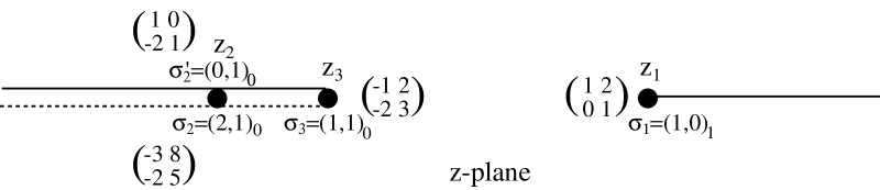
Figure 1: The analytic structure of the solution for $(a_{D},a)$. The singulatities at $z_{j}$ are represented by bullets, the solid lines correspond to the branch cuts of $a_{D}$ and the dotted line to the branch cuts of $a$. The quantum numbers $(n_{e},n_{m})_{s}$ of the particles becoming massless at the singularities, as well as the corresponding monodromy matrices, are also indicated.

We have $z_{1}>z_{3}>z_{2}$. We choose the position of the branch cut for the logarithm appearing in the asymptotics (3.2) in such a way that it does not disturb the analytic structure of the pure gauge theory. This is the most natural choice, since the existence of a singularity at a scale $m>>\Lambda$ cannot influence the physics at scale $\Lambda$. In Figure 1 are also indicated the quantum numbers of the particles becoming massless. Note that due to a “democracy” between the dyons [15, 13, 14], the most general choices for the electric and magnetic charges of these states are

$$\sigma_{1}=(1,0),\enspace\sigma_{2}=(n_{e}+1,1),\enspace\sigma_{2}^{\prime}=(n_{e}-1,1),\enspace\sigma_{3}=(n_{e},1),$$ (17)

where $\sigma_{j}$ corresponds to the singularity $z_{j}$ and $n_{e}$ is any integer. Our choice is $n_{e}=1$. Note also that due to the cuts, the particle becoming massless at $z_{2}$ is described by two different sets of integers, $\sigma_{2}$ or $\sigma_{2}^{\prime}$, depending on whether one looks from the $\mathop{\Im m}\nolimits z<0$ or $\mathop{\Im m}\nolimits z>0$ half-plane. This shows that one must introduce two different monodromy matrices at $z_{2}$,

$$M_{2}=M_{(2,1)}=\pmatrix{-3&8\cr-2&5\cr},\enspace{\mathrm{a}nd}\enspace M_{2}^{\prime}=M_{(0,1)}=\pmatrix{\hfill 1&0\cr-2&1\cr}.$$ (18)

The other monodromy matrices are

$$M_{1}=M_{(1,0)}=\pmatrix{1&2\cr 0&1\cr},\quad M_{3}=M_{(1,1)}=\pmatrix{-1&2\cr-2&3\cr}.$$ (19)

It is now possible to study the transformation properties of $(a_{D},a)$ (or equivalently of $(n_{e},n_{m})_{s}$) under duality. The naive guess would be that $(a_{D},a)$ transforms exactly according to the corresponding SL$(2,{\tencop Z})$ matrix $D$ acting on the parameters of the microscopic theory as in (14). However, we will see that this is not true in general. We must introduce an SL$(2,{\tencop Z})$ matrix $D_{\mathrm{e}ff}$ which acts on the low energy effective action (i.e. $a_{D}$ and $a$) while $D$ acts on the microscopic parameters. This subtlelty stems from the fact that the monodromy group associated with the curve (9) is $\Gamma(2)$, the subgroup of SL$(2,{\tencop Z})$ consisting in the matrices congruent to the identity modulo 2. The only straightforward and correct statement that can be done is thus that $D_{\mathrm{e}ff}=D$ mod 2. Moreover, in the massive theories, $a_{D}$ and $a$ can also pick up some constants under a duality transformation. This is allowed by the form of the BPS mass formula (2,3), since a shift in $a_{D}$ or (and) $a$ can be reabsorbed in a shift of $s$. A very similar and related phenomenon occurs when one is studying the duality transformations of the low energy theory [8, 16], but one must keep in mind that by now we are studying duality transformations of the whole, microscopic, theory.

Let us be more concrete. What we want to deduce is a formula relating the dual theory solution characterised by the parameters $(z^{D},\tau^{D},m^{D})$ given by (14) and whose periods are

$$a_{D}^{D}(z,\tau,m) = a_{D}(z^{D},\tau^{D},m^{D}),$$

$$a^{D}(z,\tau,m) = a(z^{D},\tau^{D},m^{D}),$$ (20)

to the original solution described by $(a_{D}(z,\tau,m),a(z,\tau,m))$. Let us focuss in this Section on the transformation $D=S$. The analytic structure of $(a_{D}^{D},a^{D})$ can be readily deduced from the one of $(a_{D},a)$ depicted in Figure 1. Indeed, as $E_{1}(-1/\tau)=\tau^{2}E_{2}(\tau)$, $E_{2}(-1/\tau)=\tau^{2}E_{1}(\tau)$ and $E_{3}(-1/\tau)=\tau^{2}E_{3}(\tau)$, the effect of the duality transformation will simply be to exchange the singularities at $z_{1}$ and $z_{2}$ while the singularity at $z_{3}$ remains fixed. The dual theory thus has singularities at exactly the same points as the original theory (a direct consequence of the self-duality of the curve (9)), but the quantum numbers of the states becoming massless at a given point, as well as the position of the branch cuts, are changed, see Figure 2.

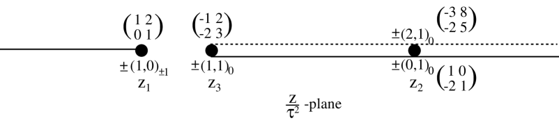
Figure 2: The analytic structure of the dual theory. It should be compared with the one of the original theory depicted in Figure 1.

This is enough to deduce that

$${\mathrm{f}or}\enspace\mathop{\Im m}\nolimits z>0 \,:\, \left\{\begin{array}[]{l}\displaystyle a_{D}(z,-1/\tau,m)=a(z/\tau^{2},\tau,m)-2a_{D}(z/\tau^{2},\tau,m)+{m\over\sqrt{2}}\\ \displaystyle a(z,-1/\tau,m)=-a_{D}(z/\tau^{2},\tau,m)+{m\over\sqrt{2}}\\ \end{array}\right.$$ (23)

$${\mathrm{a}nd\ for}\enspace\mathop{\Im m}\nolimits z<0 \,:\, \left\{\begin{array}[]{l}\displaystyle a_{D}(z,-1/\tau,m)=-a(z/\tau^{2},\tau,m)+{m\over\sqrt{2}}\\ \displaystyle a(z,-1/\tau,m)=a_{D}(z/\tau^{2},\tau,m)-2a(z/\tau^{2},\tau,m)+{m\over\sqrt{2}}\cdotp\\ \end{array}\right.$$ (26)

The shifts by $m/\sqrt{2}$ come from the fact that a dyon is exchanged with a quark, and these two states have different $s$. Moreover, the S duality transformation does not simply exchange $a$ and $a_{D}$ (up to a sign, and up to the shifts). This is not surprising since the state becoming massless at $z_{3}$ is $(1,1)$ in both formulations, and this state is not self-dual (is not an eigenvector of S). Second, to eliminate the cut between $z_{3}$ and $z_{1}$ in the dual formulation (and thus recover the same structure for the cuts as in the original formulation), it is necessary to perform an SL$(2,{\tencop Z})$ transformation, given on one side of the cut by the monodromy $M_{(0,1)}$. This also explains why the transformation law depends on the sign of $\mathop{\Im m}\nolimits z$.

3.3 Implications of S duality on the dyon spectrum

We are by now in a position to state precisely what the duality $\tau\rightarrow-1/\tau$ implies for the dyon spectrum. These predictions will be tested in the following.

At a very general level, suppose you postulate that the theories described by the variables $(a_{D},a)$ and $(\tilde{a}_{D},\tilde{a})$ are equivalent. If

$$\pmatrix{\tilde{a}_{D}\cr\tilde{a}\cr}=M\pmatrix{a_{D}\cr a\cr}+{m\over\sqrt{2}}\,\Sigma^{\prime} \quad\Longleftrightarrow\quad \pmatrix{a_{D}\cr a\cr}=M^{-1}\pmatrix{\tilde{a}_{D}\cr\tilde{a}\cr}-{m\over\sqrt{2}}\,\Sigma$$

$$\Sigma^{\prime} = M\Sigma,$$ (28)

where $M$ is an SL$(2,{\tencop Z})$ matrix and $\Sigma$ and $\Sigma^{\prime}$ are ${\tencop Z}^{2}$-valued constant sections (this is the most general transformation law we will encounter), then the existence of a state $\sigma=(n_{e},n_{m})$ of charge $s$ in the theory $(a_{D},a)$ will imply the existence of a state $\sigma^{\prime}=(n_{e}^{\prime},n_{m}^{\prime})$ of charge $s^{\prime}$ in the theory $(\tilde{a}_{D},\tilde{a})$ with

$$\sigma^{\prime}=M\sigma,\enspace s^{\prime}=s+\sigma\cdot\Sigma=s+\sigma^{\prime}\cdot\Sigma^{\prime}.$$ (29)

The $\cdot$ product denotes the standard symplectic product,

$$(p,q)\cdot(r,s)=ps-qr.$$ (30)

The formula (29) is a straighforward consequence of the BPS mass formula (2).

Let us apply (29) to the S transformation $\tau\rightarrow-1/\tau$ described by (23). Suppose that you have a state $(n_{e},n_{m})_{s}$ in the theory at given $z$, $\tau$ and $m$. This state may be a vector or a hyper multiplet of $N=2$ supersymmetry, and lie in a given representation of the flavour group. Then S duality gives a prediction for the spectrum of the theory whose parameters are $(\tau^{2}z,-1/\tau,m)$. If $\mathop{\Im m}\nolimits z>0$, we must have there a state $(-2n_{e}+n_{m},-n_{e})_{s+n_{m}-n_{e}}$, in a similar $N=2$ multiplet as the original state. The flavour quantum numbers may be changed as discussed in Section 2.2. If $\mathop{\Im m}\nolimits z<0$, the state predicted by duality will be $(-n_{m},n_{e}-2n_{m})_{s+n_{m}-n_{e}}$.

It is very important to realize that these predictions of duality relate theories having different parameters, even at the self-dual point $\tau=-1/\tau$. Thus a priori they say nothing about the dyon spectrum of a given theory (i.e., at fixed $z$, $\tau$ and $m$). One may be tempted to argue that, due to the stability of the BPS states, the parameters can be varied continuously without changing the spectrum. This means that a state which exists in the theory $(\tau^{2}z,-1/\tau,m)$ will also exist in the theory $(z,\tau,m)$. This reasoning is indeed correct when $m=0$, but is wrong in the massive case, due to the presence there of curves of marginal stability, accross which otherwise stable BPS states become degenerate in mass with multiparticle states. On these curves, the decay of BPS states is possible. We will investigate these decays in the following. Their mere existence implies that the self-duality of a general $N=2$ theory does not entail that the spectrum of BPS states is self-dual at a given point on the moduli space.

3.4 A first grasp of the dyon spectrum

Let us now penetrate at the heart of our problem: is there an easy way to understand why the spectra of the massless theories should be self-dual? Can we readily imagine what the spectrum of the massive theories look like?

There is a regime where the second question can be easily answered, at least partially. By choosing the parameters as indicated in (5), we can integrate out the quarks having a bare mass, and we are thus left with the pure gauge theory (for SO(3)) or with the SU(2) theory with two massless flavours. The spectra of these theories are well-known [13, 14]. Discarding for the moment the states having $s\not=0$, which can have arbitrarily high physical masses when $m\rightarrow\infty$, two regions in the Coulomb branch must be distinguished. Indeed, to the possible decays of $s=0$ states into other $s=0$ states corresponds a unique curve of marginal stability ${\cal C}=\{\mathop{\Im m}\nolimits(a_{D}/a)=0\}$ which looks like an ellipse and contains the singularities $z_{2}$ and $z_{3}$ [25, 13], see Figure 3.

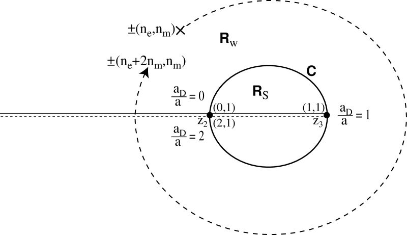
Figure 3: The curve of marginal stability $\cal C$ for the pure gauge theory or for the $N_{f}=2$ massless theory. The branch cuts as well as some values of the ratio $a_{D}/a$ are indicated. The path encircling the singularities used in the main text is also represented.

It can be shown that inside the curve (in the strong coupling region ${\cal R}_{\mathrm{S}}$) only the two BPS states which become massless at $z_{2}$ or at $z_{3}$ can be present [13, 14]. These are $\pm(1,1)_{0}$ and $\pm(0,1)_{0}\equiv\pm(2,1)_{0}$ (for this latter state, two different descriptions in terms of electric and magnetic quantum numbers are necessary, due to the non trivial analytic structure [13, 14]). Outside the curve, in what we call the weak coupling region ${\cal R}_{W}$, the BPS spectrum can be understood in different ways. The most natural certainly is to perform a semiclassical analysis, which is valid here because of asymptotic freedom (in the context of the full, finite, theory, this means that we are considering a region of the Coulomb branch where $\Lambda^{2}\ll\langle{\mathrm{t}r}\,\phi^{2}\rangle\ll m^{2}$). This analysis first tells you that the perturbative states, created by the fundamental fields, must be present. In the SO(3) theory, we have the W bosons $\pm(1,0)_{0}$ and the photon $(0,0)_{0}$ which lie in vector multiplets. In the $N_{f}=2$ theory we again have the W bosons, now represented as $\pm(2,0)_{0}$, the photon, but also the elementary quarks $\pm(1,0)_{1}$ and $\pm(1,0)_{-1}$. Beyond this perturbative spectrum, we have a solitonic spectrum. In the one monopole sector, we can construct all the states $(n_{e},1)$. The fact that all the integers $n_{e}$ are realized simply comes from the quantization of the periodic zero mode associated with electric charge rotations. Statements about higher magnetic charges would be much harder to do. It was shown in [10] that no state with $n_{m}=2$ exists, but a complete analysis for $|n_{m}|\geq 3$ seems by now impossible, for the explicit form of the multimonopole metric is not known in general in these cases. However, there is another method, initiated in [13], which consists in remarking first that the spectum in ${\cal R}_{W}$ must be invariant under the transformation

$$(n_{e},n_{m})\,\longrightarrow\,(n_{e}+2n_{m},n_{m}).$$ (31)

This can be shown by transporting the state $(n_{e},n_{m})$ along a closed path encircling the two singularities and which does not cross $\cal C$, so that the state remains stable (see Figure 3). In this operation, we cross the cut $z<z_{2}$ and thus should perform an analytic continuation of the periods $a_{D}$ and $a$ in order to insure that the physical mass of the state varies continuously. An analytic continuation $(\tilde{a}_{D},\tilde{a})$ across a cut will in general be related to the main solution $(a_{D},a)$ by a relation of the form (3.3) ($\Sigma^{\prime}$ is indeed ${\tencop Z}^{2}$-valued because the residues of the Seiberg-Witten differential form are $\pm m/\sqrt{2}$, see Appendix A). This shows that a state represented by $(n_{e},n_{m})_{s}$ on the one side of the cut will be represented by $(\tilde{n}_{e},\tilde{n}_{m})_{\tilde{s}}$ on the other side, see (29). For the cut $z<z_{2}$, we will have $\Sigma=0$ and $M=M_{3}M_{2}$ (or the inverse matrix depending on whether we turn clockwise or counterclockwise), which indeed generates the transformation (31). Since the states $(1,1)$ and $(0,1)$ must be present (they are responsible for the singularities), we immediately deduce that all the states $(n_{e},1)$ are also present, for any integer $n_{e}$. The reader might think that this is really a roundabout mean to show that electric charge is quantized. However, this reasoning also provides a statement about the $|n_{m}|\geq 2$ sectors, powerful enough to show that no state with $|n_{m}|\geq 2$ can exist. Indeed, if such a state $(n_{e},n_{m})$ would exist, it would be associated with the whole tower of states $(n_{e}+2kn_{m},n_{m})$, for any integer $k$, and one of these states will inevitably becomes massless somewhere on the curve $\cal C$ since $a_{D}/a$ takes all real values between 0 and 2 on this curve [13]. This would produce an additional singularity on the Coulomb branch which does not exist.

The greatest virtue of this kind of reasoning is that one can generalize it to other cases. We have just studied the RG flow (5) towards the pure gauge (or $N_{f}=2$) theory. It would be as natural to study the S dual of this RG flow, which would correspond to

$$4m^{4}q^{D}(\tau)=\Lambda^{4},\quad m\rightarrow\infty,\quad q^{D}\rightarrow 0,$$ (32)

where

$$q^{D}(\tau)=e^{-2i\pi/\tau}.$$ (33)

This is inherently a strong coupling limit where the semiclassical method cannot be applied. The solution for the dual pure gauge (or massless $N_{f}=2$) theory is given by $(a_{D}^{D},a^{D})$, and its analytic structure has already been worked out, see Figure 2. It is of course very tempting to try to repeat the analysis already made for the original theory. However, we cannot generalize the reasoning at once because the position of the branch cuts are now completely different. The fact that we will nevertheless obtain a spectrum in complete accordance with duality is a nice evidence that S duality is indeed correct.

3.5 Study of the dual pure gauge theory and of the dual $N_{f}=2$ massless theory

The aim of this subsection is to work out the BPS spectra implied by the analytic structure depicted in Figure 2. It is convenient to use, instead of $(a_{D}^{D},a^{D})$, the periods

$$\alpha_{D}=a_{D}^{D}-{m\over\sqrt{2}}\raise 2.0pt\hbox{,}\enspace\alpha=a^{D}-{m\over\sqrt{2}}\cdotp$$ (34)

This simply amounts to setting $s$ to zero for the two states $(1,0)$ and $(1,1)$ becoming massless. We will note with an uppercase $D$ the $s$ charge computed with the new variables,

$$s^{D}=s+n_{m}-n_{e}.$$ (35)

We have again a curve of marginal stability ${\cal C}^{D}=\{\mathop{\Im m}\nolimits(\alpha_{D}/\alpha)=0\}$, which coincides with $\cal C$ because of (23).

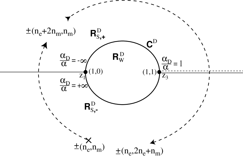
Figure 4: The Coulomb branch of the dual pure gauge (or $N_{f}=2$) theory obtained in the limit (32), separated into the two regions ${\cal R}_{W}^{D}$ and ${\cal R}_{S}^{D}$ by the curve of marginal stability ${\cal C}^{D}$. The branch cuts, the quantum numbers of the particles becoming massless, and the value of $\alpha_{D}/\alpha$ at some points of ${\cal C}^{D}$ are indicated, as well as the name of the different regions. This configuration is the dual of the one displayed in Figure 3.

The Coulomb branch is thus separated into two regions. The one inside the curve will be called in this context the weak coupling region ${\cal R}_{W}^{D}$ and is the dual of the strong coupling region ${\cal R}_{S}$ one had previously. Outside the curve, we will have the strong coupling region ${\cal R}_{S}^{D}$. These names deserve some comments. In any case, one should keep in mind that the bare gauge coupling of the whole (finite) theory is very large in the limit (32). Thus, by strong or weak coupling, we only refer to the effective coupling which governs the low energy physics. Moreover, even in ${\cal R}_{W}^{D}$ for instance, the effective theory may be strongly coupled (it is near $z_{3}$ since there a magnetically charged particle is massless). The point is that the regions in ${\cal R}_{W}^{D}$ where the coupling is strong can always be joined to other regions in ${\cal R}_{W}^{D}$ where the coupling is weak, the dyon spectrum remaining unchanged. Indeed, the electric effective coupling is zero at $z_{1}$ where the quark is massless. This suggests that the BPS spectrum might be probed in the vicinity of $z_{1}$ by using standard, “semiclassical,” approximation schemes, since we do have in this region a small parameter in the original, “electric,” theory. Actually, if duality is correct (and we will prove that its predictions indeed are concerning the dyon spectrum), the physics should be the same in the weakly coupled region surrounding $z_{1}$ in Figure 4 as in the strongly coupled region surrounding $z_{2}$ in Figure 3, and we should be able to account for the “strong coupling” jumps of the BPS spectrum seen in [13, 14] by using such methods. However, we will not try to do that here.

Let us rather apply our method to the weak coupling spectrum ${\cal S}_{W}^{D}$. It contains of course the states $(1,1)$ and $(1,0)$, which are responsible for the singularities and thus exist on both sides of the curve. We will now show that no other state, having $s^{D}=0$, can exist. This can be understood by studying the variations of $\alpha_{D}/\alpha$ along the curve ${\cal C}^{D}$. $\alpha_{D}/\alpha$ is related to $a_{D}/a$ by the formulas (34) and (23), and $a_{D}/a$ varies monotonically from 0 to 2 when one follows ${\cal C}^{D}$ clockwise starting from and ending at the singularity where $(1,0)$ is massless. This immediately implies that $\alpha_{D}/\alpha$ takes all values between $-\infty$ and 1 in the upper half plane, and all values between 1 and $+\infty$ in the lower half plane. Thus any state $(n_{e},n_{m})$ existing in ${\cal R}_{W}^{D}$ will become massless somewhere on ${\cal C}^{D}$, at the point where $\alpha_{D}/\alpha=n_{e}/n_{m}$, and then must be either $(1,0)$ or $(1,1)$. This is in perfect agreement with S duality.

When looking at the strong coupling spectrum, the complications come from the fact that one must consider analytic continuations across the cuts $z\geq z_{3}$ and $z\leq z_{1}$. We then need to introduce two different descriptions ${\cal S}^{D}_{S,+}$ and ${\cal S}^{D}_{S,-}$ in terms of electric and magnetic quantum numbers of the same physical spectrum ${\cal S}_{S}^{D}$, depending on whether we are in the upper or lower half plane. This is satisfactory from the point of view of duality, see Section 3.3. Quantitatively, a state $(n_{e},n_{m})$ in ${\cal R}^{D}_{S,-}$ will be $M_{1}(n_{e},n_{m})=(n_{e}+2n_{m},n_{m})$ after crossing the cut $z\leq z_{1}$ and $M_{3}^{-1}(n_{e},n_{m})=(3n_{e}-2n_{m},2n_{e}-n_{m})$ after crossing the cut $z\geq z_{3}$. By looping around the curve of marginal stability, taking care of remaining in ${\cal R}^{D}_{S}$, we thus immediately deduce that ${\cal S}^{D}_{S,-}$ must be invariant under the subgroup of SL$(2,{\tencop Z})$ generated by $M_{3}M_{1}$:

$${\cal S}^{D}_{S,-}=(M_{3}M_{1})^{p}{\cal S}^{D}_{S,-}=(-1)^{p}\pmatrix{1&0\cr 2p&1\cr}{\cal S}^{D}_{S,-},\quad p\in{\tencop Z}.$$ (36)

Applying this transformation to the states $(1,0)$ and $(1,1)$, which we know must exist, will then generate states having any magnetic charge:

$$\{\pm(1,p),p\in{\tencop Z}\}\in{\cal S}_{S,-}^{D}\leftrightarrow\{\pm(1+2p,p),p\in{\tencop Z}\}\in{\cal S}_{S,+}^{D}.$$ (37)

Actually, this shows that all the states dual to the $(n_{e},1)$ states of the original theory will be present. Moreover, to each state $(n_{e},1)$ corresponds one and only one state in the dual theory, since there the states are in one to one correspondence with states becoming massless. Are there any other states with $s^{D}=0$? If so, let $(n_{e},n_{m})$ be such a state in $\cal R_{S,-}^{D}$. If $n_{m}=0$, it is the state $(1,0)$ which indeed exists for it is responsible for one of the singularity. Otherwise, let us consider the ratio $r_{0}=n_{e}/n_{m}$. This ratio necessarily is in the interval $]-\infty,1[$, since otherwise the corresponding state would become massless somewhere on the curve ${\cal C}^{D}$ (note that we are working in the lower half plane and thus we see only half of the curve). As explained above, in the upper half plane the same state is described by other electric and magnetic quantum numbers. Crossing the cut $z>z_{3}$, we will obtain another ratio $\tilde{r}_{0}=(3r_{0}-2)/(2r_{0}-1)$, which must be in the interval $]1,+\infty[$ unless the particle becomes massless somewhere on the Coulomb branch. One can return in the lower half plane by crossing the cut $z<z_{1}$, and obtain again a new ratio $r_{1}$. By repeating this operation, we obtain two homographic sequences $r_{n}$ and $\tilde{r}_{n}$,

$$r_{n} = {r_{0}\over 1-2r_{0}n}$$

$$\tilde{r}_{n} = {(3+4n)r_{0}-2\over(2+2n)r_{0}-1}\raise 2.0pt\hbox{,}$$ (38)

with the following important property: if, for some $n\in{\tencop Z}$, $r_{n}\in[1,+\infty[$ or $\tilde{r}_{n}\in]-\infty,1]$, then the state $(n_{e},n_{m})$ we started from must be one of the states already obtained above (see (37)). It is elementary to check that this is always the case, except if $r_{0}=0$. This case corresponds, in the SO(3) theory, to the dual of the W bosons, and is represented by $\pm(0,1)$ in ${\cal R}^{D}_{S,-}$ and by $\pm(2,1)$ in ${\cal R}^{D}_{S,+}$. In the $N_{f}=4$ theory, we would again have, in ${\cal R}^{D}_{S,-}$, the state $\pm(0,1)$, now interpreted as being the dual of the elementary quarks, and also $\pm(0,2)$, interpreted as being the dual of the W.

Up to now, we did not take into account eventual decays of $s^{D}=0$ states into $s^{D}\not=0$ states along the path depicted in Figure 4, although this path can cross curves of marginal stability corresponding to such decays. However, the states $s^{D}\not=0$ have a mass of order $m$, whereas the states $s^{D}=0$ are likely to have a mass of order $\Lambda$ in the region surrounding the singularities $z_{3}$ and $z_{1}$ we are considering. Since in the RG flow, $m\rightarrow\infty$ while $\Lambda$ is fixed, the decays are impossible and the curves of marginal stability simply indicate that the inverse decay reaction from a $s^{D}\not=0$ to a $s^{D}=0$ state is possible. One might put forward the fact that states having $s^{D}\not=0$ but arbitrarily high electric and magnetic charges could have a mass of order $\Lambda$ due to a subtle compensation of the terms $n_{m}\alpha_{D}-n_{e}\alpha$ and $ms^{D}/\sqrt{2}$ in the BPS mass formula. However such fine tuning, which is indeed possible, can only occur for some very special values of $n_{e}$ and $n_{m}$ and in some very special and small regions in the $z$-plane. Nothing prevents us to avoid these special points and to cross the curve of marginal stability nearby, where the $s^{D}\not=0$ state again have a mass of order $m$. I wish here to point out that, though we have considered the possibility of these “fine tuning” points, they are very likely to be unphysical. Indeed, if states producing these “fine tuning” points would exist, the theory would not have a well defined field theory limit under the (dual) RG flow.

We have thus obtained the following results: states with any magnetic charges, dual to the dyons $n_{m}=1$, indeed exist, with the correct multiplicities. Thus, though the positions of the branch cuts are completely different in the original and in the dual theories, the deduced spectra are perfectly compatible with duality. However, we have not yet proven that the states corresponding to $r_{0}=0$ are really present; we simply know that they may be. This point will be investigated in Appendix B.

4 Self-dual field theories?

4.1 General discussion

In the preceding Section, we have shown using simple arguments that stable states having any magnetic charge, which are required by S duality, indeed exist. We were studying theories with non zero bare masses, but it is very tempting to think that these states can be continuously deformed while remaining stable when $m\rightarrow 0$ and thus are at the origin of the existence of states having any magnetic charge in the massless theories as well. However, we will not obtain in this process all the states required by duality in the massless theories. For instance in the SO(3) ($N=4$) theory S duality implies the existence of all the states $(n_{e},n_{m})$ with $n_{e}$ and $n_{m}$ relatively prime. Up to now, we only have the states $(q,n_{m})$ with $q=1$, and it is not difficult to realize in the context of the semiclassical approach [11] that once you have one of these states, then you will also have all the other states $(1+kn_{m},n_{m})$, for any integer $k$. Actually, the missing states should come from configurations where states having any $n_{e}$ and $n_{m}$ relatively prime are massless at the singularities. The fact that such configurations must exist is clearly a necessary condition for the self-duality of the theories, and does not follow straightforwardly from the SL$(2,{\tencop Z})$ invariance of the curve (9). We saw above that for any imaginary value of $\tau$ ($\theta=0$), the singularities are produced by states having $|n_{m}|=0$ or $|n_{m}|=1$ alone. One must then study cases where $\mathop{\Re e}\nolimits\tau\not=0$ and find a mechanism to understand how the quantum numbers at the singularities can change. This is similar to a phenomenon which is known to occur for instance in the massive SU(2) asymptotically free theories, where semiclassical quarks must “transmute” into monopoles in order to account for the singularity structure at strong coupling [8]. However, there can be an important difference between this kind of transmutation and the one we will see at work below. We will realize that two kinds of transmutations can occur. In the first kind, the quantum numbers of the state are changed according to a matrix of the form (8). We will see in the next subsections that this is the only kind of transmutation that can occur in the theories under study in this paper, because singularities in the moduli space never coincide, see (16). In the second kind of transmutation, the state transforms according to a matrix which is not of the form (8) (note that, in any case, there are many of them, since the matrices (8) are all conjugate to some power of $T$). These transmutations of the second kind are directly related to the necessity for two (or more) singularities to coincide for some special values of the parameters [32]. These special points are known to lead to superconformal theories [26].

Let us come back to our problem. We will soon show that the quantum numbers at the singularities can only be changed by matrices belonging to the monodromy group $\cal G$ (in the cases under study, we will see that any matrix of ${\cal G}=\Gamma(2)$ can be generated). It is also clear that a necessary condition for the theories to be self-dual is that any state, related to the original states becoming massless by a duality group transformation, must become massless for some value of the coupling. If the $\sigma_{j}$ denote the electric and magnetic quantum numbers of the particles becoming massless in the original configuration, we see that the theory can be self-dual only if

$${\cal G}\{\sigma_{j}\}={\cal D}\{\sigma_{j}\},$$ (39)

where ${\cal D}$ denotes the duality group. For our purposes, ${\cal G}=\Gamma(2)/\{\pm 1\}$, ${\cal D}={\mathrm{S}L}(2,{\tencop Z})$, $\{\sigma_{j}\}=\{(1,0);(2,1);(1,1)\}$ and ${\cal D}\{\sigma_{j}\}=\{(p,q),p\wedge q=1\}$. We thus have to check whether any $(p,q)$, $p$ and $q$ relatively prime, can be generated by acting with a $\Gamma(2)$ matrix on one of the three states $(0,1)$, $(1,1)$ or $(2,1)$. This is indeed true because SL$(2,{\tencop Z})/\Gamma(2)\sim S_{3}$ and that $S_{3}$ is generated by three transpositions whose corresponding matrices (already described mod 2 in Section 2.2.2) can be chosen in order to map a “fundamental” state, say $(1,0)$, exactly into the three states $(1,0)$, $(1,1)$ and $(2,1)$ we have at our disposal.

4.2 The transformation $\tau\rightarrow\tau/(2\tau+1)$

Let us start from a configuration, characterized by a certain value of the bare coupling $\tau_{0}$ and of the bare mass $m$, and whose analytic structure is of the same type as the one described in Figure 1. We will allow the monodromy matrices $M_{j}$ to be of the most general form, provided they satisfy the fundamental consistency conditions

$$M_{2}^{\prime}M_{3}M_{1}=M_{1}M_{3}M_{2}=-1.$$ (40)

To these monodromy matrices correspond states becoming massless, characterized by their electric and magnetic quantum numbers $\sigma_{j}=(p_{j},q_{j})$ and $s$-charge $s_{j}$. Note that (40) implies via (8), amongst other relations of the same type,

$$\sigma_{3}\cdot\sigma_{2}=(\sigma_{3}\cdot\sigma_{1})(\sigma_{1}\cdot\sigma_{2}).$$ (41)

Actually, as we will only consider configurations which are SL$(2,{\tencop Z})$ transforms of the original one depicted in Figure 1, SL$(2,{\tencop Z})$ symplectic invariant relations can be checked or deduced using $\sigma_{1}=(1,0)$, $\sigma_{2}=(2,1)$, $\sigma_{2}^{\prime}=(0,1)$ and $\sigma_{3}=(1,1)$. Some useful ones are

$$\sigma_{1}\cdot\sigma_{3}=1,\enspace\sigma_{2}=\sigma_{3}+\sigma_{1},\enspace\sigma_{2}^{\prime}=\sigma_{3}-\sigma_{1}.$$ (42)

We must also have

$$\sigma_{2}^{\prime}=M_{3}\sigma_{2},\enspace M_{2}^{\prime}=M_{3}M_{2}M_{3}^{-1},\enspace s_{2}^{\prime}=s_{2}+2s_{3}\sigma_{3}\cdot\sigma_{2}.$$ (43)

Now, let us vary continuously $\tau$ from $\tau_{0}$ to $\tau_{1}=\tau_{0}/(2\tau_{0}+1)$. During this operation, the singularities, and with them the branch cuts, will move on the Coulomb branch, as depicted in Figure 5.

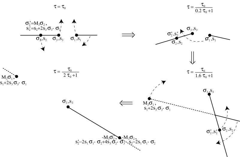
Figure 5: Different steps in the analytic continuation from $\tau=\tau_{0}$ to $\tau=\tau_{1}=\tau_{0}/(2\tau_{0}+1)$. The picture is drawn for $\tau_{0}=i$, $\tau=\tau_{0}/(2\tau_{0}t+1)$, $0\leq t\leq 1$, and $m$ real. The branch cuts are represented by solid or dotted lines depending whether they lie on the original $\tau=\tau_{0}$ sheet or not.

Unavoidably, the singularity at $z_{1}$ will cross the cut $[z_{2},z_{3}]$; at this moment its quantum numbers are changed. According to (7,29), we will have

$$\sigma_{1}\rightarrow M_{3}\sigma_{1},\enspace M_{1}\rightarrow M_{3}M_{1}M_{3}^{-1},\enspace s_{1}\rightarrow s_{1}+2s_{3}\sigma_{3}\cdot\sigma_{1}.$$ (44)

The cut originating at $z_{1}$ will also sweep up one of the two singularities, and then change the quantum numbers there. We choose to change the singularity at $z_{2}$ (see Figure 5) because it is the only case which leads to an analytic structure at $\tau=\tau_{1}$ which is perfectly similar to the one at $\tau_{0}$, and this is convenient for our purposes. The ambiguity associated with the position of the branch cut originating at $z_{1}$ is further discussed in the next subsection. As $\sigma_{2}$ sees the original cut produced by $\sigma_{1}$, whereas $\sigma_{2}^{\prime}$ sees the cut produced by $M_{3}\sigma_{1}$, we will have

$$\sigma_{2} \rightarrow M_{1}^{-1}\sigma_{2},\enspace M_{2}\rightarrow M_{1}^{-1}M_{2}M_{1},\enspace s_{2}\rightarrow s_{2}-2s_{1}\sigma_{1}\cdot\sigma_{2}$$

$$\sigma_{2}^{\prime} \rightarrow M_{3}M_{1}^{-1}M_{3}^{-1}\sigma_{2}^{\prime},\enspace M_{2}^{\prime}\rightarrow M_{3}M_{1}^{-1}M_{3}^{-1}M_{2}^{\prime}M_{3}M_{1}M_{3}^{-1},$$ (45)

$$\hskip 142.26378pts_{2}^{\prime}\rightarrow s_{2}^{\prime}-2(s_{1}+2s_{3}\sigma_{3}\cdot\sigma_{1})M_{3}\sigma_{1}\cdot\sigma_{2}^{\prime}.$$

Finally, by using the consistency relations (40,41,43), we see that at $\tau=\tau_{1}$ we are in essentially the same configuration as at $\tau=\tau_{0}$, up to a $M_{3}$ transformation and to a rotation and dilatation in the $z$ plane. Quantitatively we have

$$\pmatrix{a_{D}\cr a\cr}\Bigl{(}(2\tau+1)^{2}z,{\tau\over 2\tau+1},m\Bigr{)}=-M_{3} \pmatrix{a_{D}\cr a\cr}\Bigl{(}z,\tau,m\Bigr{)}+$$ (46)

$$\qquad 2{m\over\sqrt{2}}\,\Bigl{(}(s_{1}+s_{3})\sigma_{3}-s_{3}\sigma_{1}\Bigr{)}.$$

Thus we have shown that we can change the quantum numbers of the singularities with the matrix $M_{3}$ (the $s$ charges being also changed according to (29)).

4.3 The transformation $\tau\rightarrow\tau+2$

Performing $M_{3}$ transformations is not enough to prove SL$(2,{\tencop Z})$ invariance. We need an additional transformation, which can be found by studying the analytic continuation $\tau\rightarrow\tau+2$ exactly along the lines of the preceding subsection. We will not repeat this argument here, but we will rather introduce another idea, which is maybe more heuristic, but has the merit of showing that the structure of the low energy effective action can imply the equivalence of theories related by some transformations of the monodromy group. We will elaborate more on this kind of argument in Section 8.

The point is that by sweeping up the $z$ plane with the branch cut originating at $z_{1}$, as shown in Figure 6, we can generate the transformation:

$$\pmatrix{a_{D}\cr a\cr}\longrightarrow M_{1}\pmatrix{a_{D}\cr a\cr}-2\,{m\over\sqrt{2}}\,s_{1}\sigma_{1}.$$ (47)

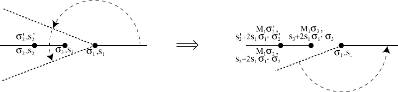
Figure 6: By sweeping up the $z$ plane with the branch cut originating at $z_{1}$, which is represented by dashed lines in intermediate positions, we generate a $M_{1}$ transformation.

Doing this on the original configuration of Figure 1 is innocent since it will generate a trivial $T^{2}$ transformation, which is interpreted as an unphysical relabelling of the electric quantum numbers $n_{e}$. It simply corresponds to a shift in the $\theta$ angle, which when combined with the change in $n_{e}$ will leave the physical electric charge and other physical observables unchanged. This shows that the position of the branch cut originating at $z_{1}$ is purely conventional when $M_{1}=T^{2}$, and by continuity this ambiguity should be preserved even when the $M_{1}$ matrix is general (we will see in the next subsection that any $M_{1}$ conjugated to $T^{2}$ by a $\Gamma(2)$ matrix can be generated by analytic continuation). Note that we performed the transformation at fixed $z$, $\tau$ and $m$. In the original configuration where $M_{1}=T^{2}$, this renders very explicit the fact that the transformation $\theta\rightarrow\theta+4\pi$ is unphysical. This also shows that the physical interpretation of the parameter $\tau$ is no longer the same after analytic continuation: if we choose to still use $\tau$ even after the $\theta$ angle shift, the real part of $\tau$ clearly will no longer be $\theta/(2\pi)$ (or $\theta/\pi$). This is even more striking when $M_{1}$ is general. Then, the transformation mixes the electric and magnetic charges in a non trivial way, still at fixed $\tau$. This is not contradictory to the Dirac quantization condition. Again, this shows that the duality transformation associated with $M_{1}$ links together two theories which are physically equivalent and thus can be labelled by the same parameters. Of course, the physical interpretation of $\tau$ in the two equivalent theories will not be the same. Similar remarks also apply to $z$. To close this discussion, note that the ambiguity in the interpretation of $\tau$ we deal with in this subsection is related to the fact already mentioned in subsection 3.2 that the SL$(2,{\tencop Z})$ matrix $D_{\mathrm{e}ff}$ which acts on $(a_{D},a)$ coincides with the SL$(2,{\tencop Z})$ matrix $D$ which acts on $\tau$ and $z$, only up to monodromy transformations. This suggests that $\tau$ can only be defined modulo $\Gamma(2)$ and thus that the structure of the low energy effective action implies that the theory has at least an exact $\Gamma(2)$ duality symmetry. We will see in Section 8 that this can be understood on physical grounds, at least heuristically.

4.4 Generating $\Gamma(2)$

Let us come back to our original problem: can we generate any $\Gamma(2)$ transformation (up to a sign) by combining the two elementary transformations (46,47) described in the previous subsections and that we will denote abstractly $t_{3}$ and $t_{1}$? Suppose that we execute the following sequence of transformations,

$$t_{3}^{q_{n}}t_{1}^{p_{n}}t_{3}^{q_{n-1}}t_{1}^{p_{n-1}}\ldots t_{3}^{q_{1}}t_{1}^{p_{1}},$$ (48)

starting from the configuration where the monodromy matrices are given by (18,19). One must take care of the fact that, after each step, the monodromy matrices are conjugated by the corresponding transformation. For instance, the transformation $t_{1}^{p_{1}}$ will indeed generate a $M_{1}^{p_{1}}$ transformation on the variables $a_{D}$ and $a$. However, the $t_{3}^{q_{1}}$ transformation that follows will be implemented by the matrix $M_{1}^{p_{1}}M_{3}^{q_{1}}M_{1}^{-p_{1}}$, since the monodromy at $z_{3}$ is no longer $M_{3}$ but $M_{1}^{p_{1}}M_{3}M_{1}^{-p_{1}}$. The effect of conjugating the matrices at each step is simply to reverse the order of the transformations in (48) to which correspond, up to a sign, the SL$(2,{\tencop Z})$ matrix

$$M_{1}^{p_{1}}M_{3}^{q_{1}}M_{1}^{p_{2}}M_{3}^{q_{2}}\ldots M_{1}^{p_{n}}M_{3}^{q_{n}}.$$ (49)

Here $M_{1}$ and $M_{3}$ are fixed matrices given by (18,19). We are thus able to obtain any matrix of the subgroup of SL$(2,{\tencop Z})$ generated by $M_{1}$ and $M_{3}$. This is just $\Gamma(2)$ as we need to prove the self duality of the spectrum, as explained at the end of Section 4.1.

The $s$ charges of the $(n_{e},n_{m})$ states obtained above can also be easily computed, by evaluating the product (49) where the monodromy matrices $M_{1}$ and $M_{3}$ are replaced by the corresponding elements of the full monodromy group, which is the semi-direct product ${\tencop Z}^{2}\times{\mathrm{S}L}(2,{\tencop Z})$ (see (47) and (46)):

$$(-2\sigma_{1},M_{1})^{p_{1}}(2\sigma_{3},-M_{3})^{q_{1}}\ldots(-2\sigma_{1},M_{1})^{p_{n}}(2\sigma_{3},-M_{3})^{q_{n}}.$$ (50)

If

$$(n_{e},n_{m})=M_{1}^{p_{1}}(-M_{3})^{q_{1}}\ldots M_{1}^{p_{n}}(-M_{3})^{q_{n}}\sigma_{j},$$ (51)

then $s=n_{e}-n_{m}$ for $j=1$ or 3, $s=-1+n_{e}-n_{m}$ for $j=2$ and $s=1+n_{e}-n_{m}$ for $j=2^{\prime}$.

4.5 Comparison with other approaches

In order to put the present work into some perspective, I will briefly discuss below some relations with other approaches.

Let me first explain how our line of reasoning can shed light on some aspects of the semiclassical quantization. I will illustrate this point on the following example. It is well known in the context of the semiclassical approach [18] that the existence of dyon-monopole bound states with $|n_{m}|\geq 2$ in the pure $N=2$ gauge theory would violate the self-duality of the $N=4$ theory. This is due to the fact that such bound states are in one to one correspondence with the cohomology classes of holomorphic differentials on the reduced ($4n_{m}-4$ dimensional) multimonopole moduli space in the case of the pure gauge theory, while the differentials only need to be harmonic in the case of $N=4$. This means that any $|n_{m}|\geq 2$ bound state of the pure gauge theory corresponds to $\em two$ bound states in the $N=4$ theory, the second state corresponding to the antiholomorphic partner of the original holomorphic differential form. This is in contradiction with $S$ duality which predicts the existence of one and only one bound state of given $n_{e}$ and $n_{m}$. From our point of view, this seemingly purely technical relation between the two theories comes from the fact that they can be joined together by continuously varying the bare mass and the coupling and using the renormalization group flow. Stable states in the pure gauge theory will then yield stable states in the $N=4$ theory, by continuous deformation. Moreover, we do not want any additional $|n_{m}|\geq 2$ state in the $N=4$ theory coming from the pure gauge theory, since we know that such states originate from the existence of dual pure gauge theories configurations.

I wish now to point out one surprising aspect of our derivation, and trace its profound origin in superstring dualities. All our reasoning is based on a careful study of the low energy effective action of the theories. Though it is well known that the latter contains a lot of information about the massive states (encoded in the BPS mass formula (2)) in the context of $N=2$ supersymmetric theories, it might seem astonishing that it also governs the formation of all the stable bound states (coming in short multiplets). Nevertheless, this fact, which appears for the first time in [13], is supported by increasing evidence. I hope that the present paper will convince the reader that it is both understandable (if not natural) and quite general in the field theory framework. However, a deeper understanding of this phenomenon comes from string theory. There, in the framework of the heterotic-type II duality conjecture [27], you can argue that the BPS states of $N=2$ supersymmetric Yang-Mills theories correspond to a self-dual non-critical string in six dimensions wrapped along geodesics around the corresponding Seiberg-Wittern curve [28]. The metric on the curve is directly related to a particular Seiberg-Witten differential, which can in principle be computed unambiguously. As all these geometric data are contained in the low energy effective action, we understand why it completely determines the BPS spectrum. In the case of $N=4$, the low energy theory as well as the metric are trivial and the self-duality of the spectrum follows easily [29] from the assumption that the type IIB string gives rise to the $N=4$ gauge theory in some limit. The cases of some SU(2) theories, including also very recently the SO(3) theory studied in this paper, were addressed in [28, 30, 31]. The case of $N_{f}=4$ should also be within the stringy approach capabilities. Our results thus constitute non trivial tests of the string-string duality hypothesis.

5 Uniqueness of the states

We will mainly focus in this Section on the $N=4$ theory, in order to avoid tiresome repetitions. In subsection 5.3, we will nevertheless briefly point out the peculiarities of the $N_{f}=4$ theory, which do not yield any new difficulties.

5.1 Precise statement of the problem and useful remarks

As there is only one multiplet in the Hilbert space of states corresponding to the fundamental $N=4$ multiplet $(1,0)$, S duality predicts the existence of only one $N=4$ multiplet $(p,q)$. As indicated in the Table 1 of Section 2, such an $N=4$ multiplet can be decomposed into three parts characterized by their physical S charges $S_{0}$, $S_{0}+1$ and $S_{0}+2$. When $m=0$, we can use CP invariance to show that the existence of a state having $S$ implies the existence of another state having $-S$, and that in a given monopole sector $n_{m}>0$, $-n_{m}\leq S\leq n_{m}$. Uniqueness of the $(p,q)$ state would therefore imply that $S_{0}=-1$, and the three values of $S$ that should be realized correspond to the CP invariant combination $\{-1,0,1\}$. The extremal values $1$ and $-1$ correspond to states belonging to a $N=2$ hypermultiplet, while $S=0$ corresponds to a $N=2$ vector multiplet.

The $(p,q)$ states we have generated in Section 4 in the massive theory correspond to $N=2$ hypermultiplets, having a given charge $S_{H}$. Because of $N=4$ supersymmetry in the $m\rightarrow 0$ limit, these hypermultiplets will be associated to other states to form whole $N=4$ multiplets $\{S_{H},S_{H}+1,S_{H}+2\}$ or $\{S_{H}-2,S_{H}-1,S_{H}\}$. The physical $S$ charges of a state $\sigma$ must be related to the constants $s$ appearing in the central charge of the supersymmetry algebra by a relation of the form [16]

$$S=s+\sigma\cdot\Xi,$$ (52)

where $\Xi\in{\tencop Z}^{2}$. To determine $\Xi$, one can proceed as follows. When $m=0$, the solution for $a_{D}$ and $a$ is given by

$$a_{D}(z,\tau,m=0)=(\tau+1-\epsilon_{z})\sqrt{2z},\quad a(z,\tau,m=0)=\sqrt{2z},$$ (53)

where $\epsilon_{z}$ is the sign of $\mathop{\Im m}\nolimits z$. The (unphysical) cut for $a_{D}$ comes from the choice we did in Section 3 for the position of the branch cut originating at $z_{1}$ when $m\not=0$. When $m\not=0$, we will have

$$a_{D}\mathop{\sim}_{|z|\rightarrow\infty}(\tau+1-\epsilon_{z})\sqrt{2z},\quad a\mathop{\sim}_{|z|\rightarrow\infty}\sqrt{2z}.$$ (54)

However, if $\Xi\not=0$, the physical $S$ charge contributes to $a_{D}$ and $a$, even at infinity, by an amount determined by $\Xi$ in such a way that

$${m\over\sqrt{2}}\,\Xi=\lim_{|z|\rightarrow\infty}\left\{\pmatrix{(\tau+1-\epsilon_{z})\sqrt{2z}\cr\sqrt{2z}\cr}-\pmatrix{a_{D}(z,\tau,m)\cr a(z,\tau,m)\cr}\right\}\cdotp$$ (55)

$\Xi$ can then be computed straightforwardly by using the formulas for $a_{D}$ and $a$ given in Appendix A. One must note, however, that the sign of $\Xi$ remains arbitrary, since it can be changed by performing a Weyl gauge transformation. This is related to the fact that one can choose equivalently $(1,0)_{+1}$ or $(1,0)_{-1}$ to be massless at $z_{1}$ in the configuration of Figure 1. The convention we will choose hereafter is the following: $(1,0)_{+1}$ will be chosen to be massless at $z_{1}$ when $m>0$ and $(1,0)_{-1}$ when $m<0$ (we will only consider real values of $m$). These conventions will allow us to use the gauge invariance in a convenient way. Finally, we have

$$\Xi=(-\epsilon_{z}\epsilon_{m},0),\enspace S=s+\epsilon_{m}\epsilon_{z}n_{m},$$ (56)

where $\epsilon_{m}$ is the sign of $m$. This formula implies in particular that the dyons found in Section 3 by studying the dual RG flow (32) all have $S=\pm 1$ as expected. It is not disturbing that $S$ may undergo a discontinuity from $\mathop{\Im m}\nolimits z>0$ to $\mathop{\Im m}\nolimits z<0$. This discontinuity simply reflects the ambiguity associated with CP invariance when $z$ or $\langle{\mathrm{t}r}\,\phi^{2}\rangle$ are real.

To be concrete, we will hereafter consider a particular configuration, obtained from the original configuration depicted in Figure 1 by performing the transformation $t_{3}t_{1}t_{3}$ (see Section 4), and which is described in Figure 7. This amounts to changing $a_{D}$ into $\tilde{a}_{D}=a_{D}-2a+\sqrt{2}\,m$ and $a$ into $\tilde{a}=4a_{D}-7a+2\sqrt{2}\,m$.

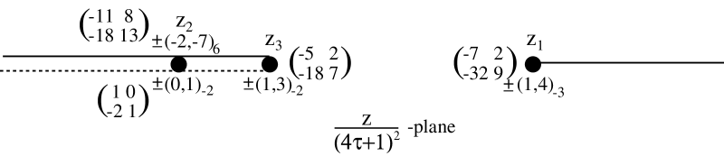
Figure 7: The configuration obtained from the one depicted in Figure 1 by performing the transformation $t_{3}t_{1}t_{3}$. With our conventions, the Figure corresponds to $m>0$.

This choice is completely arbitrary: all our reasonings will be SL$(2,{\tencop Z})$ invariant and thus completely general. However, we think that it is more eloquent to deal with states having magnetic charges three, four or seven than simply one, for in this latter case unicity of the states is trivial from the semiclassical point of view.

We already know that the $N=4$ multiplet corresponding to a state $(n_{e},n_{m})_{s}$ becoming massles is unique since the singularities are produced by only one hypermultiplet. Thus, what we need to show is that, for instance, the only allowed values of $s$ for a state $(1,4)$ should be $-3$ (charge of the hypermultiplet becoming massless) together with $-4$ and $-5$ (this would correspond to the case where the physical $S$ charge of $(1,4)_{-3}$ would be $+1$) or with $-2$ and $-1$ (when $S=-1$).

5.2 Uniqueness of the states

Suppose that a state $(1,4)_{s}$ exists in the $N=4$ theory. When a real mass $m$ is turned on, $(1,4)_{s}$ must produce a singularity at any point on the Coulomb branch where it is massless, that is where $4\tilde{a}_{D}-\tilde{a}+ms/\sqrt{2}=0$ which in the original variables reads

$$a=(4+s)\,{m\over\sqrt{2}}\cdotp$$ (57)

To study this equation, at least in the large $|s|$ limit, one can use the asymptotics (55) for $a$ at large $|z|$. This suggest that (57) might have solutions only when $s\geq-4$ when $m>0$ and only when $s\leq-4$ when $m<0$ at points

$$z_{1}^{(s)}(m)\simeq{1\over 4}(4+s)^{2}\,m^{2}.$$ (58)

More rigorously, using (65) and the monodromy $M_{1}$, one can show that $a(z)\in{\tencop R}$ for $z\geq z_{3}$. Moreover, one can easily show using the explicit formulas of $a$ and its derivative $\partial a/\partial z$ given in Appendix A that, in the case $m>0$, $a$ is a monotonically increasing function for $z\in[z_{3},+\infty[$, with $0<a(0)<m/\sqrt{2}$ (this latter value is reached at $z_{1}=z_{1}^{(1)}$), and $a\rightarrow\infty$ when $z\rightarrow\infty$. Strictly similar results are true when $m<0$, which proves that the simple analysis using the asymptotics is valid except concerning $s=-4$, as one may have expected. As the $z_{1}^{s}(m)$ exist for any $m>0$ when $s\geq-3$ and for any $m<0$ when $s\leq-5$, a singularity must be associated in the massive theories to any state $(1,4)_{s}$ existing in the massless one, provided $s\geq-3$ (if $m>0$) or $s\leq-5$ (if $m<0$). From this we deduce that when $m>0$, which corresponds to the case depicted in Figure 7, the state becoming massless at $z_{1}$, having $s=-3$, must have a physical $S$ charge $+1$ (it is thus associated with states having $s=-4$ and $s=-5$ when $m=0$), and that no other $(1,4)_{s}$ state having $s>-3$ can exist when $m=0$. When $m<0$, the state becoming massless at $z_{1}$ will have $s=-5$ and $S=-1$ and we see that no other $(1,4)_{s}$ state having $s<-5$ can exist when $m=0$. This proves the unicity.

Exactly the same reasoning can be applied to the states $(1,3)_{s}$. The equation to study is in this case

$$a_{D}-a=(s+2)\,{m\over\sqrt{2}}\cdotp$$ (59)

By using again (55), we can convince ourselves, and then show rigorously, that when $\mathop{\Im m}\nolimits z>0$ (59) will have solutions when $s<-1$ (for $m>0$) or when $s>-3$ (for $m<0$). This is again perfectly consistent with our previous analysis of the $s$ and $S$ charges. When $m>0$, it is the state having $S=-1$ which is massless, and we showed that no state $(1,3)$ with $S<-1$ can exist; when $m<0$ it is the state having $S=+1$ which is massless, and we showed that no state with $S>1$ can exist. Thus the $N=4$ multiplet $(1,3)$ is indeed unique and realizes the values $S=-1$, $S=0$ and $S=1$ as it should.

Finally, note that the case of the states $(2,7)_{s}$ and $(0,1)_{s}$ can be easily handled for instance by using the previous results and the $\tau\rightarrow-1/\tau$ type duality transformation (23), or by repeating the same analysis as above. Of course, the reasoning will not change whatever configuration of the theory you may choose, and thus we have proven the unicity of the states $(p,q)$ for any $p$ and $q$ relatively prime.

5.3 The case of $N_{f}=4$

In this theory, the solution is given by $a_{D}^{N_{f}=4}=a_{D}/2$ and $a^{N_{f}=4}=a/2$, and the bare masses of the first and second flavours are equal to $m/2$. The uniqueness of the $(p,q)$ states can then be proven exactly as for the $N=4$ theory. In particular, a $(p,q,S)$ hypermultiplet becoming massless when $m\not=0$ will again be associated to two other sets of states having physical charges $S-1$ and $S-2$, or $S+1$ and $S+2$ when $m=0$, the Spin(8) flavour symmetry playing the same rôle in this theory as $N=4$ supersymmetry in the previous case. The main novelty is that one also has to study the uniqueness of the vector $(2p,2q)$ states. Again one can repeat the arguments of the preceding subsection. Equation (57) will be replaced by

$$a={1\over 2}\,(4+s)\,{m\over\sqrt{2}}\cdotp$$ (60)

From the analysis of the preceding subsection it follows that this equation has solutions for any $s$ such that $|s-4|\geq 2$. Moreover, by using the formula for $a$ given in Appendix A, one can show that $a(0)=|m/(2\sqrt{2})|$ when $\tau=i$ and thus the equation (60) will also have solutions for $|s-4|=1$ at least for some values of $\tau$. Thus, the only $(2p,2q)$ states, $(p,q)=(1,0)$ mod 2, that might exist in the $m=0$ theory must have $S=0$, as expected. The same reasoning works for the state $(2p,2q)$ such that $(p,q)=(0,1)$ mod 2. However, when $(p,q)=(1,1)$ mod 2, one cannot exclude directly the states having a physical $S$ charge $\pm 1$. This seems to be a peculiarity of the vector particles: at fixed $\tau$, these vector particles, if they existed, would not necessarily lead to an unphysical singularity, and hence their existence cannot be ruled out by this argument alone. Of course, this is not really an obstacle for us. By changing $\tau$ to $\tau+1$ in the original configuration, we exchange $z_{2}$ and $z_{3}$ and thus states $(p,q)=(0,1)$ mod 2 with states $(p,q)=(1,1)$ mod 2, and we can then deduce that necessarily $S=0$ for the latter states.

To prove the unicity, we still have to check whether only one state exists at given $p$, $q$ and $s$. The argument which worked for the $(p,q)$ states relied on the fact that any of these states can be related to a singularity appearing on the Coulomb branch for some values of the coupling, and that we know the multiplicity of the states producing singularities. This clearly does not work for the $(2p,2q)$ states, which are never massless (when $m\not=0$) and thus never produce a singularity. As an alternative, we will rely on a semiclassical analysis. In [10] was shown that the states $(2p,2q)$ indeed exist and are unique for $|q|=1$. The uniqueness of the $(2p,2q,S=0)$ states for any $p$ and $q$ relatively prime will then follow from the $\Gamma(2)$ invariance of the theory, see Section 8.

6 Generalities about the curves of marginal stability

Due to the BPS mass formula (2), a BPS state is generically stable. Central charge as well as mass conservation indeed impose tights constraints. To see this, suppose that a BPS state of central charge $Z$ decay into $p$ states of central charges $Z_{1},\ldots,Z_{p}$. This is possible only if

$$Z=Z_{1}+\cdots+Z_{p}$$ (61)

and

$$|Z|=|Z_{1}|+\cdots+|Z_{p}|.$$ (62)

A necessary condition for these equations to be compatible is that

$$\mathop{\Im m}\nolimits{Z_{k}\over Z}=0\enspace{\mathrm{f}or}\enspace 1\leq k\leq p.$$ (63)

Of the $p$ relations (63), only $p-1$ are independent once one takes into account (61), and thus they define a hypersurface of real codimension $p-1$ included in the Coulomb branch. In our case where the gauge group is of rank one and thus the Coulomb branch of real dimension two, this means that decays into two distinct particles can only occur along real curves, decays into three distinct particles at special points, and decays into four or more distinct particles are likely to be impossible.

Suppose we are studying the decay of a state $(\sigma,s)$ into two states, one of them being $(\sigma^{\prime},s^{\prime})$. Instead of using the original variables $\omega=(a_{D},a)$, it is convenient to use shifted variables $\Omega=(A_{D},A)$ such that $s=0$. The equation for the curve of marginal stability can then be cast in the following SL$(2,{\tencop Z})$ invariant form:

$${m\over\sqrt{2}}\,{\Omega\cdot\overline{\Omega}\over 2i\mathop{\Im m}\nolimits\overline{\Omega}\cdot\sigma}={s^{\prime}\over\sigma\cdot\sigma^{\prime}}\cdotp$$ (64)

The left hand side of (64) does not depend on the final state $(\sigma^{\prime},s^{\prime})$, and the right hand side is an a priori arbitrary rational number which we will denote by $r$. We thus see that to a given particle $(\sigma,s)$ is associated a whole family of curves of marginal stability, ${\cal C}_{(\sigma,s)}(r)$, indexed by a rational number $r$.

It is useful at this stage to summarize what we need to show in order to complete our goal, which is to demonstrate that the spectrum of BPS states is in perfect agreement with $S$ duality both in the $N=4$ and massless $N_{f}=4$ theory, and also to prove the existence of the required states in the massive cases studied in Section 3.
— We need to show that the states $(p,q)$, where $p$ and $q$ are relatively prime integers, which we have generated by analytic continuation in the massive theories (Section 4), still exist in the massless one. This will be established in Section 7 using the curves of marginal stability.
— We need to show that the states $(2p,2q)$ exist in the $N_{f}=4$ theory, since they represent the duals of the W bosons in this case. We did not give any argument in favour of the existence of such states up to now, since they are not associated with any singularity on the Coulomb branch. However, one can establish their existence by using the general argument presented in Section 8, and by relying on the non trivial semiclassical results obtained in [10] for states of magnetic charge 2.
— Finally, we need to show that the dual of the W bosons (and of the elementary quarks in the $N_{f}=4$ theory) does exist in the dual theory studied in Section 3.5. There it was only shown that the existence of these states does not lead to any inconsistency. Actually, these dual states exist in the massless theories, and in Appendix B we will explain why they must still exist when the bare mass is increased and we follow the RG flow (32) toward the dual pure gauge (or massless $N_{f}=2$) theory.

Let us end this Section by mentioning the formula

$$\pmatrix{a_{D}\cr a\cr}\Bigl{(}\overline{z}\Bigr{)}=\pmatrix{-1&2\cr 0&1\cr}\pmatrix{\overline{a}_{D}\cr\overline{a}\cr}\Bigl{(}z\Bigr{)},$$ (65)

which corresponds to a CP transformation. Note that though this is not a duality transformation, it is still perfectly compatible with the BPS mass formula (2). This relation is useful to study the symmetries and some particular points of the curves of marginal stability.

7 Existence of the states $(p,q)$

In this Section, $p$ and $q$ are two relatively prime integers.

In Section 4, strong evidence in favour of the existence of the states $(p,q)$ in the massless theories was given: depending on the value of the coupling $\tau$, when the bare mass is turned on, the singularities on the Coulomb branch may be due to any of these states. However, strictly speaking, the existence of the states was proven only when $m\not=0$ and $z=z_{j}$. When $m=0$ and the singularities merge at $z=0$, all the $(p,q)$ states become massless and thus degenerate in mass. Though a brutal discontinuity in the spectrum between $m\not=0$ and $m=0$ seems very unlikely on physical grounds, we would like to argue that the $(p,q)$ states not only exist at the singularities they are responsible for, but also at other points in the $z$ plane. One way of doing this is to consider a configuration where the $(p,q)$ state becomes massless, and to study the family of curves of marginal stability associated with the decay of this state. If $(p,q)=(1,0)$ mod 2, we have a family ${\cal C}_{1}(r)$ defined by (cf (64))

$${\cal C}_{1}(r):\enspace\mathop{\Im m}\nolimits a_{D}(\overline{a}-{m\over\sqrt{2}})={m\over\sqrt{2}}\,r\,\mathop{\Im m}\nolimits a,\enspace r\in{\tencop Q}$$ (66)

and if $(p,q)=(1,1)$ mod 2 we have a family ${\cal C}_{3}(r)$,

$${\cal C}_{3}(r):\enspace\mathop{\Im m}\nolimits a_{D}\overline{a}={m\over\sqrt{2}}\,r\,\mathop{\Im m}\nolimits(a-a_{D}),\enspace r\in{\tencop Q}.$$ (67)

The case of $(p,q)=(0,1)$ mod 2 is completely similar to the case $(p,q)=(1,0)$ mod 2 due to (23). We have computed the curves ${\cal C}_{j}(r)$ numerically, using the analytic formulas for the periods presented in Appendix A, and the result is depicted in Figure 8.

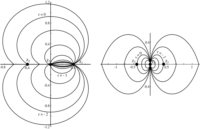
Figure 8: The families ${\cal C}_{1}(r)$ (on the left) and ${\cal C}_{3}(r)$ (on the right) for some values of $r$. The singularities at $z_{j}$ are represented by a bullet. We chose $\tau=i$ and $m=1.5$.

It is easy to established, particularly in using (65), that the curves ${\cal C}_{3}(r)$ all intersect at $z_{3}$ and are symmetric with respect to the real $z$ axis, while the curves ${\cal C}_{1}(r)$ all intersect at $z_{1}$ and $z_{3}$ and $\overline{\cal C}_{1}(r)={\cal C}_{1}(-r-\sqrt{2}m)$. More important, these curves do not intersect at any other points than the particular ones mentioned above and form a dense set in the whole $z$ plane. This is not prohibitive: the complementary set, generated by the curves ${\cal C}_{j}(x)$ for irrational values of $x$, is also a dense subset of the Coulomb branch, where the corresponding state is stable. This shows that for any positive real number $R$, there is always a point $z$ such that $|z|>R$ and which can be joined to the singularity $z_{j}$ by a curve ${\cal C}_{j}(x)$ where $x$ is taken to be irrational. As the state becoming massless at $z_{j}$ cannot decay along such a curve, it must exist at $z$. As $R$ can be chosen independently of $m$, $(p,q)$ must exist in the $m=0$ theory for some $|z|>R$ and thus for any $z$.

To end this Section, I wish to point out that the preceding analysis suggests that states which cannot exist in the $m=0$ theory cannot exist anymore in the $m\not=0$ theory. To understand this, assume that to the unwanted state $(p,q)_{s}$ is associated a point $z_{0}$ on the Coulomb branch such that

$$qa_{D}(z_{0})-pa(z_{0})+ms/\sqrt{2}=0,$$ (68)

for any given $\tau$ and $m$.. The family of curves of marginal stability ${\cal C}_{(p,q)_{s}}(r)$ associated with $(p,q)_{s}$ looks like the families depicted in Figure 8, except that all the curves will intersect at $z_{0}$. Now suppose that $(p,q)_{s}$ exist at a point on a curve ${\cal C}_{(p,q)_{s}}(x)$ with $x$ irrational (such curves cover a dense subset ${\cal E}$ of the Coulomb branch). Then move $(p,q)_{s}$ along this curve, reach $z_{0}$ where it is massless and find an inconsistency since $z_{0}$ is not a singular point. Thus $(p,q)_{s}$ cannot exist in the dense set ${\cal E}$: this means that it will never be a trully stable state in the theory. Thus, if our hypothesis (68) is correct, the number of curves of marginal stability one must consider to study eventual decays in the massive theories is considerably decreased. We will use this fact in Appendix B, see also [32].

8 The general physical argument and $\Gamma(2)$ invariance

In this Section, we wish to address a very general problem: when can we expect the monodromy group of a given theory to correspond to an exact duality symmetry? Of course, this a priori naive statement is not always true, as Seiberg and Witten already pointed out in their original paper [15] on the pure gauge theory. However, we would like it to be correct in the particular cases of the finite theories studied in this paper. We will give in the following some general physical arguments showing that this property can be understood simply by looking at some very general features of the structure of the low energy effective action. Though we will restrict ourselves to very few examples, in the framework of SU(2) gauge theories, and chosen in order to illuminate the cases of SU(2) $N=4$ and $N=2$, $N_{f}=4$, the line of reasoning could a priori be applied to any $N=2$ theory.

First, let us consider a theory with only one singularity on the Coulomb branch. It could be the massless theories studied above. Let us see why in this simple case, the monodromy $M$ associated with this singularity must correspond to an exact duality symmetry of the theory. To the singularity is associated a branch cut which extends to infinity and whose orientation clearly is arbitrary. By sweeping up the $z$ plane with such a branch cut, while keeping all the parameters fixed, we show that necessarily two theories connected by the transformation $M$ must be physically equivalent. This kind of argument was already presented in subsection 4.3. In the case of $N=4$ or $N=2$ with four massless flavours, $M=-I$ and the “duality” transformation is nothing but a gauge transformation.

Let us now go to a more interesting situation, suited for instance for the pure gauge theory, where two singularities are present at $z_{1}$ and $z_{2}$ with monodromies $M_{1}$ and $M_{2}$. The theory now has an intrinsic scale $\Lambda$ such that $|z_{2}-z_{1}|=\Lambda^{2}$. Two scenarios can be imagined in this case. In the first one, for some reasons the naive arguments are true, and thus the monodromy group generated by $M_{1}$ and $M_{2}$ corresponds to an exact duality symmetry. In the second scenario, the two singularities combine: we choose the branch cut originating at $z_{1}$ to go through $z_{2}$ and then to coincide with the branch cut originating at $z_{2}$. Far away from the singularities, we thus only see a branch cut associated with a monodromy matrix $M_{\infty}$ which is the product of the two matrices $M_{1}$ and $M_{2}$. Of course the position of this branch cut extending to infinity can be chosen arbitrarily, and thus an exact duality symmetry must be associated with $M_{\infty}$, at least when $|z|>>\Lambda^{2}$. In the case of the pure gauge theory, $M_{\infty}$ expresses the asymptotic freedom and is associated with the invariance of the theory under $\theta$ angle shifts.

Finally, let us study the case where three singularities $z_{j}$ are present on the Coulomb branch, with monodromy matrices $M_{j}$. The theory may now have one, two, or three intrinsic scales, corresponding to the distances $|z_{j}-z_{k}|$ between the singularities. In the $N=2$ theory with one flavour of quark, we have three singularities at equal distances from each other because of a ${\tencop Z}_{3}$ symmetry acting on the Coulomb branch [15, 14]. Thus we have only one scale $\Lambda$ at our disposal. The same scenario as the one which prevailed for the pure gauge theory occurs, and we do not have any particular duality symmetry in this theory. Now, the finite theories we are studying in this paper also have three singularities in the Coulomb branch, but with the most important property that two independent scales can be introduced and any one of the three singularities can be chosen to be arbitrarily far from the other two. Typically, we are studying a dual RG flow as in (32), and two of the three singularities (say $z_{1}$ and $z_{2}$) are separated by an almost fixed distance $\Lambda^{2}$ while the third singularity ($z_{3}$) runs to infinity with $m$ at a distance $m^{2}$, where $m$ is the bare mass in the theory. In such a configuration, as in the case where only two singularities are present, we cannot know a priori whether the monodromies $M_{1}$ and $M_{2}$ associated with the singularities at scale $\Lambda$ will correspond to an exact duality symmetry. However, the situation is different for the isolated singularity at scale $m$. The latter can only be “screened” by the singularities at scale $\Lambda$. We think that this is impossible, because it seems very unlikely that the low energy physics at scale $\Lambda$ could be influenced by a singularity at scale $m$, produced by a particle which is ultra massive at scale $\Lambda$ (if it exists), and vice-versa. One might argue that the branch cuts of the three singularities could merge at a new intrinsic scale $\mu$. However, the physical origin of this new scale would be very unclear and we will rule out this possibility. We thus see that the only natural way to interpret the singularity structure is to admit that $M_{3}$ corresponds to an exact duality symmetry of the theory at least in the configuration where $|z_{1}-z_{2}|\sim\Lambda^{2}$ and $z_{3}\sim m^{2}$ with $m^{2}>>\Lambda^{2}$. From the point of view of the massless theory, which corresponds to $|z|>>m^{2}>>\Lambda^{2}$, we have thus an invariance with respect to $M_{3}$. The rôle of the three singularities can of course be exchanged due to the SL$(2,{\tencop Z})$ invariance of the Seiberg-Witten curve (9), and we deduce that the $m=0$ theories have an exact duality group which contains $\Gamma(2)$.

In particular, the existence of all the $(2p,2q)$ states in the $N_{f}=4$ theory will then follow from the existence of the three states $(2,0)$ (the W), $(2,2)$ and $(0,2)$, which were shown to exist in [10] using the semiclassical method.

9 Conclusion

In this paper, we proved rigorously that all the $(p,q)$ dyon states, where $p$ and $q$ are relatively prime integers, exist in the $N=4$ as well as in the $N=2$, $N_{f}=4$ gauge theories with gauge group SU(2). These states were obtained by analytic continuation of the $|q|\leq 1$ states which become massless at some points of the Coulomb branch when the bare $\theta$ angle is zero. In the process of analytic continuation, we saw explicitly that the quantum numbers at the singularities can change according to a monodromy transformation. We also proved the unicity of the dyon states, in perfect agreement with an exact SL$(2,{\tencop Z})$ duality symmetry. We also provided a very general physical argument showing that $N=4$ and $N=2$ with four massless flavours must have an exact duality symmetry group which contains the monodromy group of the corresponding massive theories. This fact together with already known semiclassical results implies the existence of all the $(2p,2q)$ vector states in the $N_{f}=4$ theory.

The line of reasoning used in this work, particularly the arguments of subsections 4.1 and 8, is likely to be generalizable to theories having any gauge group, for instance to the case of SU(N) with $N_{f}=2N$. This may answer the open questions in these cases [33].

From a very general point of view, our method may be seen as the physical counterpart of the string theory results based on the heterotic-type II duality conjecture [28]. It would be very interesting to prove the equivalence of the two approaches. In our approach, one is seeking for non singular points $z$ on the Coulomb branch and for cycles $c=(p,q)$ on the Seiberg-Witten curve $\Sigma_{z}$ such that

$$(c,\lambda)=\oint_{c}\lambda_{\mathrm{S}W}=0,$$ (69)

where $\lambda_{\mathrm{S}W}$ is the Seiberg-Witten differential form, see Appendix A. States $(p,q)$ corresponding to such a cycle $c$ cannot exist, and any other (hypermultiplet) states are very likely to exist. In the string approach, stable states are associated with geodesics on $\Sigma_{z}$ endowed with the metric $|\lambda|^{2}$ where $\lambda$ is a particular element in the cohomology class of $\lambda_{\mathrm{S}W}$. For states lying in a $N=2$ hypermultiplet, these geodesics must begin and end at the branching points $e_{j}$ (see (A.1) in Appendix A). A link between the two points of view is the following: it is clearly impossible to have a non-null geodesic with the required properties for a state $c$ satisfying (69), since the geodesic would have zero length and this requires its endpoints to coincide, that is to have a singularity. More important, the existence of a particular point $z$ such that (69) is true is likely to prevent the existence of the corresponding geodesic for “any” $z$, by continuity. Of course subtleties are associated with the curves of marginal stability, and the vector particles may have a particular status. In any case, we believe that a complete understanding of the relationship between the two approaches is likely to provide a deeper understanding of $N=2$ theories. It is a pleasure to thank Adel Bilal for his permanent encouragements and many interesting discussions. His critical reading of the manuscript was also at the origin of many improvements. I also thank Adam Schwimmer for a useful discussion, and Aurélia who kindly processed the Figures.

Appendices

Appendix A The computation of the periods

A.1 Notations and general formulas

I present below some general formulas from the theory of elliptic integrals (see, e.g., [34]) in a form well suited for our purposes. By well suited, I mean first that they can be used straighforwardly to obtain the analytic solution for $a_{D}$ and $a$. Actually, the same general formulas can be used to evaluate the periods of the asymptotically free theories having $N_{f}\leq 3$ as well [32]. Second, I mean that they can easily be implemented on a computer system, and thus can be used to determine numerically the curves of marginal stability.

Let us consider a torus whose equation is

$$y^{2}=4\prod_{j=1}^{3}\bigl{(}x-e_{j}\bigr{)}.$$ (70)

In our particular case, it will be convenient to cast (9) into this form by performing the change of variable

$$x=X-E_{1}(\tau)z-{1\over 4}m^{2}E_{1}^{2}(\tau),\enspace y=2Y.$$ (71)

We will then have

$$e_{1}(z,\tau,m) = 0,$$

$$e_{2}(z,\tau,m) = \bigl{(}E_{2}(\tau)-E_{1}(\tau)\bigr{)}z+{1\over 4}m^{2}\bigl{(}E_{2}^{2}(\tau)-E_{1}^{2}(\tau)\bigr{)},$$

$$e_{3}(z,\tau,m) = \bigl{(}E_{3}(\tau)-E_{1}(\tau)\bigr{)}z+{1\over 4}m^{2}\bigl{(}E_{3}^{2}(\tau)-E_{1}^{2}(\tau)\bigr{)}.$$ (72)

The fundamental cycles on the torus (70) are chosen as indicated in Figure A.1.

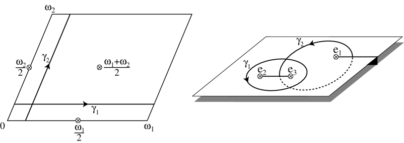
Figure 9: The fundamental cycles $\gamma_{1}$ and $\gamma_{2}$ are represented in the two cases where the torus is viewed as a two sheeted surface with branch cuts from $e_{2}$ to $e_{3}$ and from $e_{1}$ to $\infty$, or as a rectangle whose opposite edges are identified.

To this choice for the homology basis, we associate the usual variables $k$ and $k^{\prime}$:

$$k^{2}={e_{3}-e_{2}\over e_{1}-e_{2}}\raise 2.0pt\hbox{,}\quad k^{\prime 2}=1-k^{2}={e_{1}-e_{3}\over e_{1}-e_{2}}\cdotp\\$$ (73)

The fundamental periods are then given by

$$\omega_{1}(z,\tau,m) = \oint_{\gamma_{1}}{dx\over y}={2\over\sqrt{e_{1}-e_{2}}}\,K(k),$$

$$\omega_{2}(z,\tau,m) = \oint_{\gamma_{2}}{dx\over y}={2i\over\sqrt{e_{1}-e_{2}}}\,K(k^{\prime}),$$ (74)

where $K$ is the standard complete elliptic integral of the first kind. We will also need a formula involving elliptic integrals of the third kind. Maybe the most convenient form for this formula is the following:

$$\oint_{\gamma_{j}}{dx\over(x-c)y}={1\over\wp^{\prime}(u_{c})}\,\Bigl{(}2\omega_{j}\,\zeta(u_{c})-4\eta_{j}\,u_{c}+2i\ell\pi\Bigr{)},$$ (75)

where $c$ is any complex number which is different from the roots $e_{j}$ and $\ell$ is an integer. The $\eta_{j}$ are given by

$$\eta_{1} = -{1\over 2}\,\oint_{\gamma_{1}}{x\over y}\,dx=\sqrt{e_{1}-e_{2}}\,E(k)-{e_{1}\over\sqrt{e_{1}-e_{2}}}\,K(k),$$

$$\eta_{2} = -{1\over 2}\,\oint_{\gamma_{2}}{x\over y}\,dx=-i\sqrt{e_{1}-e_{2}}\,E(k^{\prime})-i{e_{2}\over\sqrt{e_{1}-e_{2}}}\,K(k^{\prime})$$ (76)

in terms of the complete elliptic integrals of the first and second kinds $K$ and $E$. $\wp$ and $\zeta$ are straightforward generalizations (note that $e_{1}+e_{3}+e_{3}\not=0$ here) of the Weirstrass $\wp$ and $\zeta$ functions, and may be expressed in terms of the standard Jacobian and $\theta$ elliptic functions [34] as

$$\wp(u;z,\tau,m) = e_{2}+{e_{1}-e_{2}\over\mathop{\rm sn}\nolimits^{2}\bigl{(}(e_{1}-e_{2})^{1/2}u,k\bigr{)}}$$

$$\wp^{\prime}(u;z,\tau,m) = -2(e_{1}-e_{2})^{3/2}\,{\mathop{\rm cn}\nolimits\bigl{(}(e_{1}-e_{2})^{1/2}u,k\bigr{)}\mathop{\rm dn}\nolimits\bigl{(}(e_{1}-e_{2})^{1/2}u,k\bigr{)}\over\mathop{\rm sn}\nolimits^{3}\bigl{(}(e_{1}-e_{2})^{1/2}u,k\bigr{)}}$$

$$\zeta(u;z,\tau,m) = {2\eta_{1}\over\omega_{1}}\,u+{1\over\omega_{1}}\,{\theta^{\prime}\over\theta}\Bigl{(}{u\over\omega_{1}}\Bigr{)}.$$ (77)

Finally, $u_{c}$ is such that $\wp(u_{c})=c$, that is

$$u_{c}=\wp^{-1}(c)={1\over\sqrt{e_{1}-e_{2}}}\,\mathop{\rm sn}\nolimits^{-1}\left[\left({e_{1}-e_{2}\over c-e_{2}}\right)^{1/2},k\right].$$ (78)

The indeterminate constant $\ell$ comes from the fact that the differential form $dx/\bigl{(}(x-c)y\bigr{)}$ has poles with residues $1/\wp^{\prime}(u_{c})$. If, under a continuous deformation, the integration contour crosses such a pole, $\ell$ will be shifted by one unit. Note also that the ambiguity that exists in the definition of $u_{c}$, which stems from the fact that $\wp(u)$ is a doubly periodic, even function of $u$, can be absorbed in a redefinition of $\ell$ by using Legendre’s relation $\eta_{1}\omega_{2}-\eta_{2}\omega_{1}=i\pi$ and the fact that $\zeta(u+n_{1}\omega_{1}+n_{2}\omega_{2})=\zeta(u)+2(n_{1}\eta_{1}+n_{2}\eta_{2})$ for any integers $n_{1}$ and $n_{2}$. It should be clear that such integrals can only appear in theories with non zero bare masses, since it is only here that jumps in $a_{D}$ and $a$ are allowed [8, 16]. Changing $\ell$ will then simply amount to shifting the $s$ charge.

We are now equipped to compute the Seiberg-Witten periods $a_{D}$ and $a$ rather straighforwardly. However, two points remain to be discussed. First, when applying the above formulas, we are not certain to obtain a solution with the correct analytic structure in the $z$ plane. This is explained in the next subsection where the effective coupling $t(z,\tau,m)$ is computed. Second, we must find the Seiberg-Witten differential, if possible in a form where the canonical decomposition in terms of the building blocks treated above is simple. This is done in subsection 5.3. The solution is then given in 5.4.

A.2 The effective coupling $t$

The effective coupling $t$ is nothing but the modular parameter of the torus (9), and would thus naively be given by $\omega_{2}/\omega_{1}$. However, this formula is a priori valid only modulo SL$(2,{\tencop Z})$ transformations, and some additional constraints must be found from physics. The first constraint comes from the evaluation of $t$ in the limit $z\rightarrow\infty$ where it should coincide with $\tau$, modulo $\theta$ angle redefinitions which correspond to trivial shifts of the electric charge. This constraint is indeed satisfied with our choices for the homology cycles $\gamma_{1}$ and $\gamma_{2}$. The second constraint comes from the analytic structure of $t$ as a function of $z$, which was described in Section 3 in the case of a trivial bare $\theta$ angle. This analytic structure is most easily studied when one uses the explicit formulas

$$k^{2}={\theta_{1}^{4}\over\theta_{3}^{4}}\,{z-z_{1}\over z-z_{3}}\raise 2.0pt\hbox{,}\quad k^{\prime 2}={\theta_{2}^{4}\over\theta_{3}^{4}}\,{z-z_{2}\over z-z_{3}},$$ (79)

and

$$e_{1}-e_{2}=(z-z_{3})\,\theta_{3}^{4},$$ (80)

where the $z_{j}$ correspond to the positions of the singularities (16). We then obtain a unique solution, given when $\theta=0$ by

$$t(z,\tau,m)={da_{D}\over da}=\left\{\begin{array}[]{lll}\omega_{2}/\omega_{1}&{\mathrm{f}or}&\enspace\mathop{\Im m}\nolimits z\geq 0.\\ \omega_{2}/\omega_{1}+2&{\mathrm{f}or}&\enspace\mathop{\Im m}\nolimits z<0.\\ \end{array}\right.$$ (81)

$\partial a_{D}/\partial z$ and $\partial a/\partial z$ are also very directly related to the fundamental periods $\omega_{1}$ and $\omega_{2}$. Before writing explicit formulas, one must note that though having the same monodromies, the solution for the SO(3) and $N_{f}=4$ theories will differ by a global factor of $1/2$ which directly comes from the analysis of the massless theories. In the following, we will reserve the notation $(a_{D},a)$ for the solution of the SO(3) theory, and for $N_{f}=4$ we will have $(a_{D}^{N_{f}=4},a^{N_{f}=4})=(a_{D}/2,a/2)$. With these conventions,

$${\partial a\over\partial z}={\sqrt{2}\over 2\pi}\,\omega_{1}={\sqrt{2}\over\pi}{1\over\theta_{3}^{2}\sqrt{z-z_{3}}}\,K(k)$$ (82)

and

$${\partial a_{D}\over\partial z}=\left\{\begin{array}[]{lll}{\displaystyle\sqrt{2}\over\displaystyle\pi}\,{\displaystyle 1\over\displaystyle\theta_{3}^{2}\sqrt{z-z_{3}}}\,iK(k^{\prime})&{\mathrm{f}or}&\enspace\mathop{\Im m}\nolimits z\geq 0.\\ {\displaystyle\sqrt{2}\over\displaystyle\pi}\,{\displaystyle 1\over\displaystyle\theta_{3}^{2}\sqrt{z-z_{3}}}\,\bigl{(}iK(k^{\prime})+2K(k)\bigr{)}&{\mathrm{f}or}&\enspace\mathop{\Im m}\nolimits z<0.\\ \end{array}\right.$$ (83)

A.3 The Seiberg-Witten differential

We now wish to integrate the relations (82,83) in order to obtain $a_{D}$ and $a$. To do this, the standard method is to find a one form $\lambda$ (the so-called Seiberg-Witten differential) so that

$${\partial\lambda\over\partial z}={dx\over dy}$$ (84)

up to an exact form. We will then compute $a_{D}$ and $a$ by mean of the formulas

$$a(z,\tau,m)={\sqrt{2}\over 2\pi}\oint_{\gamma_{1}}\lambda,\quad a_{D}(z,\tau,m)={\sqrt{2}\over 2\pi}\oint_{\gamma_{2}}\lambda.$$ (85)

The simplest way to find $\lambda$ certainly is to use, instead of the variables $(y,x)$, the rescaled variables $(\tilde{y}=y/(2\theta_{2}^{3}\theta_{3}^{3}),\,\tilde{x}=x/\theta_{2}^{2}\theta_{3}^{2})$ in terms of which the curve takes the form

$$\tilde{y}^{2}=\tilde{x}M(\tilde{x},z,\tau,m)N(\tilde{x},z,\tau,m)$$ (86)

with

$${\partial\tilde{y}^{n}\over\partial z}={1\over 2}n\tilde{y}^{n-2}\tilde{x}(M+N).$$ (87)

By multiple integration by part we then obtain

$$\int{dz\over\tilde{y}} = \int dz\,{\tilde{x}R\over\tilde{y}}\,{1\over\tilde{x}R}={\tilde{y}\over\tilde{x}R}+\int dz\,(3\tilde{y}\tilde{x}R){1\over 3\tilde{x}^{2}R^{3}}=\cdots$$ (88)

$$= {1\over\sqrt{x}}\sum_{n=1}^{\infty}{1\over 2n-1}\,\left({y\over\sqrt{x}R}\right)^{2n-1}={1\over 2\sqrt{x}}\ln{\sqrt{x}R+y\over\sqrt{x}R-y}\cdotp$$

A very convenient and simple form for $\lambda$ will then be

$$\lambda=-{\sqrt{x}\over\theta_{2}\theta_{3}}\,d\ln{\sqrt{x}R+y\over\sqrt{x}R-y}=\Bigl{(}z-z_{1}\Bigr{)}\,{2x\over y}{dx\over x+{1\over 4}m^{2}\theta_{2}^{4}\theta_{3}^{4}}.$$ (89)

A.4 The computation of $a$ and $a_{D}$

We end our computation by writing $\lambda$ in the form

$$\lambda=2\bigl{(}z-z_{1}\bigr{)}{dx\over y}-{1\over 2}m^{2}\theta_{2}^{4}\theta_{3}^{4}\bigl{(}z-z_{1}\bigr{)}{dx\over y\bigl{(}x+{1\over 4}m^{2}\theta_{2}^{4}\theta_{3}^{4}\bigr{)}}\cdotp$$ (90)

By noting that

$$\wp^{\prime 2}(u)=4\prod_{j=1}^{3}\Bigl{(}\wp(u)-e_{j}\Bigr{)},$$ (91)

we can easily compute $\wp^{\prime}(u_{c})$ with $c=-m^{2}\theta_{2}^{4}\theta_{3}^{4}$ and then apply (A.1, 75) to find the desired solution:

$$a(z,\tau,m)={\sqrt{2}\over\pi}\Bigl{[}\bigl{(}z-z_{1}\bigr{)}\,\omega_{1}+{i\over 4}m\,\bigl{(}2\omega_{1}\zeta(u_{c})-4\eta_{1}u_{c}\bigr{)}\Bigr{]},$$ (92)

and

$$a_{D}(z,\tau,m) = \left\{\begin{array}[]{l}{\displaystyle\sqrt{2}\over\displaystyle\pi}\Bigl{[}\bigl{(}z-z_{1}\bigr{)}\,\omega_{2}+{i\over 4}m\,\bigl{(}2\omega_{2}\zeta(u_{c})-4\eta_{2}u_{c}\bigr{)}\Bigr{]}\quad{\mathrm{f}or}\enspace\mathop{\Im m}\nolimits z\geq 0.\\ {\displaystyle\sqrt{2}\over\displaystyle\pi}\Bigl{[}\bigl{(}z-z_{1}\bigr{)}\,(\omega_{2}+2\omega_{1})+{i\over 4}m\,\bigl{(}2(\omega_{2}+2\omega_{1})\zeta(u_{c})-4(\eta_{2}+2\eta_{1})u_{c}\bigr{)}\Bigr{]}\\ \end{array}\right.$$ (96)

$$\hskip 227.62204pt{\mathrm{f}or}\enspace\mathop{\Im m}\nolimits z<0.$$

The different prescriptions for $\mathop{\Im m}\nolimits z\geq 0$ or for $\mathop{\Im m}\nolimits z<0$ correspond of course to a zero $\theta$ angle. The generalization to any $\theta$ angle should be clear in view of the discussion in Section 4.

Appendix B Duality in the massive theories

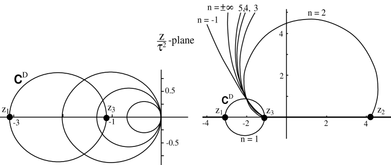
Figure 10: The curves of marginal stability corresponding to the decay of the state $(1,0)_{-1}$ (or $(2,0)_{-2}$). On the left are represented the curves ${\cal C}^{D}$ (n=1) for $\tau=i$ and various values of the mass $m$ from 0 to the RG value given by (32), and then for $m=5$ and $\tau$ given by (32). On the right, curves for $m=5$ and $\tau$ given by (32) are represented for various values of $n$.

In this Appendix, we complete the proof of Section 3 and show that the spectrum of the dual pure gauge theory (or dual $N_{f}=2$ massless theory) is in perfect agreement with duality. In Section 3, we already showed that the duals of the $|n_{m}|=1$ monopoles indeed exist outside the curve of marginal stability ${\cal C}^{D}$ represented in Figure 4 in the theory $(\tau^{2}z,-1/\tau,m)$. In addition to these states, duality predicts the existence of the duals of the W bosons, and also of the elementary quarks in the case of the $N_{f}=4$ theory. More precisely, we need to prove that in the SO(3) theory the state $(0,1)_{-1}$ indeed exists for $\mathop{\Im m}\nolimits z<0$ outside the curve ${\cal C}^{D}$ or equivalently that $(2,1)_{1}$ exists for $\mathop{\Im m}\nolimits z>0$. In the $N_{f}=4$ theory, in addition to the preceding state (now interpreted as being the dual of the quarks of the massless $N_{f}=2$ theory), we must have the $(0,2)_{-2}$ (or $(4,2)_{2}$) state interpreted as being the dual of the W.

Our strategy will be the following: as we already know that all these states exist when $m=0$, we will simply show that they cannot decay outside the curve ${\cal C}^{D}$ when the mass is turned on and we follow the RG flow (32) toward the dual pure gauge (or $N_{f}=2$) theory. To do this, remark first that the family of curves of marginal stability associated with $(0,1)_{-1}$ coincides with the one for $(0,2)_{-2}$, and that the family for $(2,1)_{1}$ is the symmetric of the family for $(0,1)_{-1}$ with respect to the real $z$ axis. Thus, we need to study only one family of curves, whose defining equations deduced from (64) can be cast in the form

$$\mathop{\Im m}\nolimits\Bigl{(}a_{D}-{m\over\sqrt{2}}\Bigr{)}\Bigl{(}\overline{a}-{m\over\sqrt{2}}\Bigr{)}=\Bigl{(}{S^{\prime}\over n_{e}^{\prime}}-1\Bigr{)}\,{m\over\sqrt{2}}\,\mathop{\Im m}\nolimits a_{D}.$$ (97)

In this equation, $S^{\prime}$ represents the physical $S$ charge a state produced in the decay reaction would have when $m=0$, and $n_{e}^{\prime}$ represents the electric charge of the same state. As argued in Section 7, we will consider only $S^{\prime}$ such that $|S^{\prime}|\leq 1$ and thus $S^{\prime}/n_{e}^{\prime}=0$ or $S^{\prime}/n_{e}^{\prime}=1/n$ where $n$ is any integer. The corresponding curves are represented in Figure B.1. As there is no curve outside ${\cal C}^{D}$ in the lower half-plane, the state $(0,1)_{-1}$ (or $(0,2)_{-2}$) cannot decay in this region. This completes the proof.

References

- [1] C. Montonen and D. Olive, Phys. Lett. B 72 (1977) 117.
-
[2]
S. Coleman, Phys. Rev. D 11 (1975) 2088
S. Mandelstam, Phys. Rev. D 11 (1975) 3026. - [3] E. Witten and D. Olive, Phys. Lett. B 78 (1978) 97.
- [4] H. Osborn, Phys. Lett. B 83 (1979) 321.
-
[5]
M.F. Sohnius and P.C. West, Phys. Lett. B 100 (1981) 245
S. Mandelstam, Nucl. Phys. B 213 (1983) 149
L. Brink, O. Lindgren and B. Nilsson, Phys. Lett. B 123 (1983) 323
M. Grisaru, M. Roček and W. Siegel, Phys. Rev. Lett. 45 (1980) 1063
P.S. Howe, K.S. Stelle and P.K. Townsend, Nucl. Phys. B 214 (1983) 519. - [6] N. Seiberg, Phys. Lett. B 206 (1988) 75.
-
[7]
A Parkes and P. West, Phys. Lett. B 122 (1983) 365
P. Howe, K. Stelle and P. West, Phys. Lett. B 124 (1983) 55
A. Parkes and P. West, Phys. Lett. B 127 (1983) 353. - [8] N. Seiberg and E. Witten, Nucl. Phys. B 431 (1994) 484.
-
[9]
L. Girardello, A. Giveon, M. Porrati and A. Zaffaroni,
Phys. Lett. B 334 (1994) 331
L. Girardello, A. Giveon, M. Porrati and A. Zaffaroni, Nucl. Phys. B 448 (1995) 127. -
[10]
S. Sethi, M. Stern and E. Zaslow, Nucl. Phys. B457 (1995) 484,
J.P. Gauntlett and J.A. Harvey, Nucl. Phys. B463 (1996) 287. -
[11]
M. Porrati, Phys. Lett. B377 (1996) 67,
G. Segal and A. Selby, Comm. Math. Phys. 177 (1996) 775. - [12] E.B. Bogomol’nyi, Sov. J. Nucl. Phys. 24 (1976) 449.
- [13] F. Ferrari and A. Bilal, Nucl. Phys. B 469 (1996) 387.
- [14] A. Bilal and F. Ferrari, Nucl. Phys. B 480 (1996) 589.
- [15] N. Seiberg and E. Witten, Nucl. Phys. B426 (1994) 19; erratum B 430 (1994) 485.
- [16] F. Ferrari, Phys. Rev. Lett. 78 (1997) 795.
-
[17]
J.P. Gauntlett, Nucl. Phys. B411 (1994) 443,
J.D. Blum, Phys. Lett. B333 (1994) 92. - [18] A. Sen, Phys. Lett. B329 (1994) 217.
-
[19]
C. Callias, Comm. Math. Phys. 62 (1978) 213,
R. Bott and R. Seeley, Comm. Math. Phys. 62 (1978) 235. - [20] E. Witten, Phys. Lett. B86 (1979) 283.
- [21] D. Finnell and P. Pouliot, Nucl. Phys. B453 (1995) 225.
-
[22]
R. Flume, M. Magro, L. O’Raifeartaigh, I. Sachs and O.
Schnetz, Nucl. Phys. B494 (1997) 331,
G. Bonelli, M. Matone and M. Tonin, Phys. Rev. D55 (1997) 6466. -
[23]
N. Dorey, V. Khoze and M. Mattis, Phys. Rev. D54 (1996)
7832,
N. Dorey, V. Khoze and M. Mattis, Nucl. Phys. B492 (1997) 607. - [24] N. Dorey, V. Khoze and M. Mattis, Phys. Lett. B396 (1997) 141.
-
[25]
A. Fayyazuddin, Mod. Phys. Lett. A10 (1995) 2703,
P.C. Argyres, A.E. Faraggi and A.D. Shapere, Curves of marginal stability in super-QCD, preprint IASSNS-HEP-94/103, UK-HEP/95-07, hep-th/9505190,
M. Matone, Phys. Rev. D53 (1996) 7354. -
[26]
P.C. Argyres and M.R. Douglas, Nucl. Phys. B448
(1995) 93
P.C. Argyres, M.R. Plesser, N. Seiberg and E. Witten, Nucl. Phys. B461 (1996) 71. - [27] C. Hull and P. Townsend, Nucl. Phys. B438 (1995) 109.
- [28] A. Klemm, W. Lerche, P. Mayr, C. Vafa and N. Warner, Nucl. Phys. B477 (1996) 746.
-
[29]
E. Witten, Some comments on string dynamics,
IASSNS-HEP-95-63, hep-th/9507121, proceedings of Strings ’95,
USC, March 1995
K. Landsteiner, E. López and D.A. Lowe, Phys. Lett. B387 (1996) 300. - [30] A. Brandhuber and S. Stieberger, Self-dual strings and stability of BPS states in SU(2) gauge theories, CERN-TH/96-263, NEIP-96/007, hep-th/9610053.
- [31] J. Schulze and N.P. Warner, BPS geodesics in supersymmetric Yang-Mills theory, USC/97-001, hep-th/9702012.
- [32] A. Bilal and F. Ferrari, The BPS spectra and superconformal points in massive N=2 supersymmetric QCD, LPTENS-97/02, hep-th/9706145.
-
[33]
O. Aharony and S. Yankielowicz, Nucl. Phys. B473 (1996) 93,
M. Cederwall and M. Holm, Monopole and dyon spectra in SYM with higher rank gauge groups, Göteborg-ITP-96-4, hep-th/9603134. - [34] K. Chandrasekharan, Elliptic functions (Springer-Verlag, Berlin, 1985).