CU-TP-812

These lectures are devoted to introducing some of the basic features of quantum geometry that have been emerging from compactified string theory over the last couple of years. The developments discussed include new geometric features of string theory which occur even at the classical level as well as those which require non-perturbative effects. These lecture notes are based on an evolving set of lectures presented at a number of schools but most closely follow a series of seven lectures given at the TASI-96 summer school on Strings, Fields and Duality.

1 Introduction

1.1 The State of String Theory

It has been about thirteen years since the modern era of string theory began with the discovery of anomaly cancellation [59]. Even though the initial euphoria of having a truly unified theory — one that includes gravity — led to premature claims of solving all of the fundamental problems of theoretical particle physics, string theory continues to show ever increasing signs of being the correct approach to understanding nature at its most fundamental level. The last two years, in particular, have led to stunning developments in our understanding. Problems that once seemed almost insurmountable have now become fully within our analytical grasp. The key ingredient in these developments is the notion of duality: a given physical situation may admit more than one theoretical formulation and it can turn out that the respective levels of difficulty in analysing these distinct formulations can be wildly different. Hard questions to answer from one perspective can turn into far easier questions to answer in another.

Duality is not a new idea in string theory. Some time ago, for instance, it was realized that if one considers string theory on a circle of radius $R$, the resulting physics can equally well be described in terms of string theory on a circle of radius $1/R$ ([58] and references therein). Mirror symmetry ([117, 62] and references therein), as we describe in these lectures, is another well known example of a duality. In this case, two topologically distinct Calabi-Yau compactifications of string theory give rise to identical physical models. The transformation relating these two distinct geometrical formulations of the same physical model is such that strong sigma model coupling questions in one can be mapped to weak sigma model coupling questions in the other. By a judicious choice of which geometrical model one uses, seemingly difficult physical questions can be analysed with perturbative ease.

During the last couple of years, the scope of duality in string theory has dramatically increased. Whereas mirror symmetry can transform strong to weak sigma model coupling, the new dualities can transform strong to weak string coupling. For the first time, then, we can go beyond perturbation theory and gain insight into the nature of strongly coupled string theory [114, 75]. The remarkable thing is that all such strong coupling dynamics appears to be controlled by one of two structures: either the weak coupling dynamics of a different string theory or by a structure which at low energies reduces to eleven dimensional supergravity. The latter is to be thought of as the low energy sector of an as yet incompletely formulated nonperturbative theory dubbed M-theory.

A central element in this impressive progress has been played by BPS saturated solitonic objects in string theory. These non-perturbative degrees of freedom are oftentimes the dual variables which dominate the low-energy structure arising from taking the strong coupling limit of a familiar string theory. Although difficult to analyze in detail as solitons, the supersymmetry algebra tells us a great deal about their properties — in some circumstances enough detail so as to place duality conjectures on circumstantially compelling foundations. The discovery of $D$-branes as a means for giving a microscopic description of these degrees of freedom [95] has subsequently provided a powerful tool for their detailed investigation — something that is at present being vigorously pursued.

Our intent in these lectures is to describe string compactification from the basic level of perturbative string theory on through some of the most recent developments involving the nonperturbative elements just mentioned. The central theme running through our discussion is the way in which a universe based on string theory is described by a geometrical structure that differs from the classical geometry developed by mathematicians during the last few hundred years. We shall refer to this structure as quantum geometry.

1.2 What is Quantum Geometry?

Simply put, quantum geometry is the appropriate modification of standard classical geometry to make it suitable for describing the physics of string theory. We are all familiar with the success that many ideas from classical geometry have had in providing the language and technical framework for understanding important structures in physics such as general relativity and Yang-Mills theory. It is rather remarkable that the physical properties of these fundamental theories can be directly described in the mathematical language of differential geometry and topology. Heuristically, one can roughly understand this by noting that the basic building block of these mathematical structures is that of a topological space — which itself is a collection of points grouped together in some particular manner. Pre-string theories of fundamental physics are also based on a building block consisting of points — namely, point particles. That classical mathematics and pre-string physics have the same elementary constituent is one rough way of understanding why they are so harmonious. Thinking about things in this manner is particularly useful when we come to string theory. As the fundamental constituent of perturbative string theory is not a point but rather a one-dimensional loop, it is natural to suspect that classical geometry may not be the correct language for describing string physics. In fact, this conclusion turns out to be correct. The power of geometry, however, is not lost. Rather, string theory appears to be described by a modified form of classical geometry, known as quantum geometry, with the modifications disappearing as the typical size in a given system becomes large relative to the string scale — a length scale which is expected to be within a few orders of magnitude of the Planck scale, $10^{-33}cm$.

We should stress a point of terminology at the outset. The term quantum geometry, in its most precise usage, refers to the geometrical structure relevant for describing a fully quantum mechanical theory of strings. In the first part of these lectures, though, our focus will be upon tree level string theory — that is, conformal field theory on the sphere — which captures novel features associated with the extended nature of the string, but does so at the classical level. As such, the term quantum geometry in this context is a bit misleading and a term such as “stringy” geometry would probably be more appropriate. In the later lectures, we shall truly include quantum effects into our discussion through some of the non-perturbative solitonic degrees of freedom, mentioned above. Understanding the geometrical significance of these quantum effects finally justifies using the term quantum geometry. To understand this distinction a bit more completely, we note that scattering amplitudes in perturbative string theory can be organized in a manner analogous to the loop expansion in ordinary quantum field theory [93]. In field theory, the loop expansion is controlled by $\hbar$, with an $L$-loop amplitude coming with a prefactor of $\hbar^{L-1}$. In string theory, the role of loops is played by the genus of the world sheet of the string, and the role of $\hbar$ is played by the value of the string coupling $g_{s}$. At any given genus in this expansion, we can analyze the contribution to a string scattering amplitude by means of a two-dimensional auxiliary quantum field theory on the genus-$g$ world sheet. This field theory is controlled by the inverse string tension $\alpha^{\prime}$ (or more precisely, the dimensionless sigma model coupling $\alpha^{\prime}/R^{2}$ with $R$ being a typical radius of a compactified portion of space, as we shall discuss below in detail). The limit of $\alpha^{\prime}\rightarrow 0$ corresponds to an infinitely tense string which thereby loses all internal structure and reduces, in effect, to a structureless point particle. Thus, in string theory there are really two expansions: the quantum genus expansion and the sigma model expansion.

	SPECIAL RELATIVITY	QUANTUM FIELD THEORY
	CLASSICAL DYNAMICS	QUANTUM MECHANICS
${v/c}~{}\uparrow$
$~{}~{}~{}~{}~{}~{}~{}~{}~{}\rightarrow$
$~{}~{}~{}~{}~{}~{}~{}~{}~{}\hbar$

Figure 1: The deformation from classical dynamics to quantum field theory.

We can summarize these two effects through a diagram analagous to one relevant for understanding the relationship between non-relativistic classical mechanics and quantum field theory [36]. The latter is summarized by figure 1.

We see that the horizontal axis corresponds to $\hbar$ (or more precisely, $\hbar$ divided by the typical action of the system being studied), while the vertical axis corresponds to $v/c$. In string theory (which we take to incorporate relativity from the outset), as just explained, there are also two relevant expansion parameters, as shown in figure 2.

Here we see that the horizontal axis corresponds to the value of the string coupling constant, while the vertical axis corresponds to the value of the sigma model coupling constant. In the extreme $\alpha^{\prime}=g_{s}=0$ limit, for instance, we recover relativistic particle dynamics. For nonzero $g_{s}$ we recover point particle quantum field theory. For $g_{s}=0$ and nonzero $\alpha^{\prime}$ we are studying classical string theory. In general though, we need to understand the theory for arbitrary values of these parameters.

	CLASSICAL STRINGY	QUANTUM STRINGY
	GEOMETRY	GEOMETRY
	CLASSICAL RIEMANNIAN	QUANTUM RIEMANNIAN
	GEOMETRY	GEOMETRY
${\alpha^{\prime}/R^{2}}~{}\uparrow$
$~{}~{}~{}~{}~{}~{}~{}~{}~{}~{}~{}~{}~{}\rightarrow$
$~{}~{}~{}~{}~{}~{}~{}~{}~{}~{}~{}~{}g_{s}$

Figure 2: The deformation from classical Riemannian geometry to quantum stringy geometry.

An important implication of the duality results briefly discussed in the last section is that any such decomposition into those physical effects due to strong string coupling or strong sigma model coupling, etc. is not invariant. Rather, strong/weak duality transformations together with various geometric dualities can completely mix these effects together. What might appear as a strong coupling phenomenon from one perspective can then appear as a weak coupling phenomenon in another. More generally, the values of string and sigma model couplings can undergo complicated changes in the course of duality transformations. The organization of figure 2 is thus highly dependent on which theoretical description of the underlying physics is used.

Having made our terminology clear, we will typically not be overly careful in our use of the term quantum vs. stringy geometry; often we shall simply use the former allowing the context clarify the precise meaning.

The discovery of the profound role played by extended solitonic objects in string theory has in some sense questioned the nature of the supposedly foundational position of the string itself. That is, since string theory contains degrees of freedom with more (and less) than one spatial dimension, and since in certain circumstances it is these degrees of freedom which dominate the low-energy dynamics (as we shall see later), maybe the term ‘string’ theory is a historical misnomer. Linguistic issues aside, from the point of view of quantum geometry it is important to note that the geometrical structure which one sees emerging from some particular situation can depend in part on precisely which probe one uses to study it. If one uses a string probe, one quantum geometrical structure will be accessed while if one uses, for instance, a $D$-brane of a particular dimension, another geometry may become manifest. Thus, quantum geometry is an incredibly rich structure with diverse properties of greater or lesser importance depending upon the detailed physical situation being studied. In these lectures we will study the quantum geometry which emerges from fundamental string probes and also from nontrivial $D$-brane configurations. We shall not discuss the quantum geometry that arises from using $D$-brane scattering dynamics; for this the reader can consult the lectures of Polchinski [95] and Shenker of this school.

As we shall see, when the typical size in a string compactification does not meet the criterion of being sufficiently large, the quantum geometry will shall find differs both quantitatively and qualitatively from ordinary classical geometry. In this sense, one can think of string theory as providing us with a generalization of ordinary classical geometry which differs from it on short distance scales and reduces to it on large distance scales. It is the purpose of these lectures to discuss some of the foundations and properties of quantum geometry.

1.3 The Ingredients

Recent developments in string theory have taken us much closer to understanding the true nature of the fully quantized theory. Rather surprisingly, it appears that perturbative tools — judiciously used — can take us a long way. In these lectures we shall focus on the tools necessary for analysing string theory in perturbation theory as well as for incorporating certain crucial nonperturbative elements. Our aim in this section is to give a brief overview of perturbative string theory in order to have the language to describe a number of recent developments.

As discussed in Ooguri’s lectures [93], it is most convenient to formulate first quantized string theory in terms of a 2-dimensional quantum field theory on the world sheet swept out by the string. The delicate consistency of quantizing an extended object places severe constraints on this 2-dimensional field theory. In particular, the field theory must be a conformal field theory with central charge equal to fifteen.

More precisely, we will always discuss type IIA or IIB superstring theory, in which case the field theory must be superconformally invariant. (Without loss of clarity, we will often drop the prefix super.) In fact, the study of these string theories leads us naturally to focus on two-dimensional field theories with two independent supersymmetries on the world sheet(on the left and on the right) and hence we discuss $N=2$ (or $(2,2)$ as it is sometimes written) superconformal field theories with central charge (both left and right) equal to fifteen. From a spacetime point of view, the corresponding effect theory governing string modes has $N=2$ supersymemtry as well. The constrained structure of $N=2$ theories has allowed us to hone a number of powerful tools which greatly aid in their understanding. We can thus push both our physical and our mathematical analysis of these theories quite far.

Our study of perturbative string theories with space-time supersymmetry thus boils down to a study of 2-dimensional $N=2$ superconformal field theories with central charge fifteen. How do we build such field theories? We will study this question in some detail in the ensuing sections; for now let us note the typical setup. In studying these string models, we will generally assume that the underlying $N=2,~{}c=15$ conformal theory can be decomposed as the product of an $N=2,~{}c=6$ theory with an $N=2$, $c=9$ theory. The former can then be realized most simply via a free theory of two complex chiral superfields, (as we will discuss explicitly shortly) — that is, a free theory of four real bosons and their fermionic superpartners. We can interpret these free bosons as the four Minkowski space-time coordinates of common experience. The $c=9$ theory is then an additional “internal” theory required by consistency of string theory. Whereas we were directly led to a natural choice for the $c=6$ theory, there is no guiding principle which leads us to a preferred choice for the $c=9$ theory from the known huge number of possibilities. The simplest choice, again, is six free chiral superfields — that is, six free bosons and their fermionic superpartners. Together with the $c=6$ theory, this yields ten dimensional flat space-time — the arena of the initial formulation of superstring theory. In this case the “internal theory” is of the same form as the usual “external theory” and hence, in reality, there is no natural way of dividing the two. Thus, for many obvious reasons, this way of constructing a consistent string model is of limited physical interest thereby supplying strong motivation for seeking other methods. This problem — constructing (and classifying) $N=2$ superconformal theories with central charge 9 to play the role of the internal theory — is one that has been vigorously pursued for a number of years. As yet there is no complete classification but a wealth of constructions have been found.

The most intuitive of these constructions are those in which six of the ten spatial dimensions in the flat space approach just discussed are “compactified”. That is, they are replaced by a small compact six dimensional space, say $M$ thus yielding a space-time of the Kaluza-Klein type $M_{4}\times M$ where $M_{4}$ is Minkowski four-dimensional space. It is crucial to realize that most choices for $M$ will not yield a consistent string theory because the associated two-dimensional field theory — which is now most appropriately described as a non-linear sigma model with target space $M_{4}\times M$ — will not be conformally invariant. Explicitly, the action for the internal part of this theory is

$$S = {1\over 4\pi\alpha^{\prime}}\int dzd{\overline{z}}\,\Big{[}g_{mn}(\partial X^{m}{\overline{\partial}}X^{n}+\partial X^{n}{\overline{\partial}}X^{m})+B_{mn}(\partial X^{m}{\overline{\partial}}X^{n}-\partial X^{n}{\overline{\partial}}X^{m})+\cdots\Big{]}~{},~{}~{}~{}~{}$$

where $g_{mn}$ is a metric on $M$, $B_{mn}$ is an antisymmetric tensor field, and we have omitted additional fermionic terms required by supersymmetry whose precise form will be given shortly.

To meet the criterion of conformal invariance, $M$ must, to lowest order in sigma model perturbation theory, admit a metric $g_{\mu\nu}$ whose Ricci tensor $R_{\mu\nu}$ vanishes. In order to contribute nine to the central charge, the dimension of $M$ must be six, and to ensure the additional condition of $N=2$ supersymmetry, $M$ must be a complex Kähler manifold. These conditions together are referred to as the ‘Calabi-Yau’ conditions and manifolds $M$ meeting them are known as Calabi-Yau three-folds (three here refers to three complex dimensions; one can more generally study Calabi-Yau manifolds of arbitrary dimension known as Calabi-Yau $d$-folds). We discuss some of the classical geometry of Calabi-Yau manifolds in the next section. A consistent string model, therefore, with four flat Minkowski space-time directions can be built using any Calabi-Yau three-fold as the internal target space for a non-linear supersymmetric sigma model. If we take the typical radius of such a Calabi-Yau manifold to be small (on the Planck scale, for instance) then the ten-dimensional space-time $M_{4}\times M$ will effectively look just like $M_{4}$ (with the present level of sensitivity of our best probes) and hence is consistent with observation à la Kaluza-Klein. We will have much to say about these models shortly; for now we note that there are many Calabi-Yau three-folds and each gives rise to different physics in $M_{4}$. Having no means to choose which one is “right”, we lose predictive power.

Calabi-Yau sigma models provide one means of building $N=2$ superconformal models that can be taken as the internal part of a string theory. There are two other types of constructions that will play a role in our subsequent discussion, so we mention them here as well. A key feature of each of these constructions is that at first glance neither of them has anything to do with the geometrical Calabi-Yau approach just mentioned. Rather, each approach yields a quantum field theory with the requisite properties but in neither does one introduce a curled up manifold. The best way to think about this is that the central charge is a measure of the number of degrees of freedom in a conformal theory. These degrees of freedom can be associated with extra spatial dimensions, as in the Calabi-Yau case, but as in the following two constructions they do not have to be.

Landau-Ginzburg effective field theories have played a key role in a number of physical contexts. For our purpose we shall focus on Landau-Ginzburg theories with $N=2$ supersymmetry. Concretely, such a theory is a quantum field theory based on chiral superfields (as we shall discuss) that respects $N=2$ supersymmetry and has a unique vacuum state. From our discussion above, to be of use this theory must be conformally invariant. A simple but non-constructive way of doing this is to allow an initial non-conformal Landau-Ginzburg theory to flow towards the infrared via the renormalization group. Assuming the theory flows to a non-trivial fixed point (an assumption with much supporting circumstantial evidence) the endpoint of the flow is a conformally invariant $N=2$ theory. More explicitly, the action for an $N=2$ Landau-Ginzburg theory can be written

$$\int d^{2}zd^{4}\theta\,K(\Psi_{1},\overline{\Psi}_{1},...,\Psi_{n},\overline{\Psi}_{n})+\left(\int d^{2}zd^{2}\theta\,W(\Psi_{1},...,\Psi_{n})+{\rm h.c.}\right)~{},$$

where the kinetic terms are chosen so as to yield conformal invariance and where the superpotential $W$, which is a holomorphic function of the chiral superfields $\Psi_{i}$, is at least cubic so the $\Psi_{i}$ are massless. (Any quadratic terms in $W$ represent massive fields that are frozen out in the infrared limit.)

By suitably adjusting the (polynomial) superpotential $W$ governing these fields we can achieve central charge nine. More importantly, along renormalization group flows, the superpotential receives nothing more than wavefunction renormalization. Its form, therefore, remains fixed and can thus be used as a label for those theories which all belong to the same universality class. The kinetic term $K$, on the contrary, does receive corrections along renormalization group flows and thus achieving conformal invariance amounts to choosing the kinetic term correctly. We do not know how to do this explicitly, but thankfully much of what we shall do does not require this ability.

The final approach to building suitable internal $N=2$ theories that we shall consider is based upon the so called “minimal models”. As we shall discuss in more detail in the next section, a conformal theory is characterized by a certain subset of its quantum field algebra known as primary fields. Most conformal theories have infinitely many primary fields but certain special examples — known as minimal models — have a finite number. Having a finite number of primary fields greatly simplifies the analysis of a conformal theory and leads to the ability to explicitly calculate essentially anything of physical interest. For this reason the minimal models are often referred to as being “exactly soluble”. The precise definition of primary field depends, as we shall see, on the particular chiral algebra which a theory respects. For non-supersymmetric conformal theories, the chiral algebra is that of the conformal symmetry only. In this case, it has been shown that only theories with $c<1$ can be minimal. One can take tensor products of such $c<1$ theories to yield new theories with central charge greater than one (since central charges add when theories are combined in this manner). If our theory has a larger chiral algebra, say the $N=2$ superconformal algebra of interest for reasons discussed, then there are analogous exactly soluble minimal models. In fact, they can be indexed by the positive integers $P\in{\mathbb{Z}}$ and have central charges $c_{P}=3P/(P+2)$. Again, even though these values of the central charge are less than the desired value of nine, we can take tensor products to yield this value. (In fact, as we shall discuss, it is not quite adequate to simply take a tensor product. Rather we need to take an orbifold of a tensor product.) In this way we can build internal $N=2,~{}c=9$ theories that have the virtue of being exactly soluble. It is worthwhile to emphasize that, as in the Landau-Ginzburg case, these minimal model constructions do not have any obvious geometrical interpretation; they appear to be purely algebraic in construction.

In the previous paragraphs we have outlined three fundamental and manifestly distinct ways of constructing consistent string models. A remarkable fact, which will play a crucial role in our analysis, is that these three approaches are intimately related. In fact, by varying certain parameters we can smoothly interpolate between all three. As we shall see, a given conformal field theory of interest typically lies in a multi-dimensional family of theories related to each other by physically smooth deformations. The paramter space of such a family is known as its moduli space. This moduli space is naturally divided into various phase regions whose physical description is most directly given in terms of one of the three methods described above (and combinations thereof) as well as certain simple generalizations. Thus, for some range of parameters, a conformal field theory might be most naturally described in terms of a non-linear sigma model on a Calabi-Yau target space, for other ranges of parameters it might most naturally be described in terms of a Landau-Ginzburg theory, while for yet other values the most natural description might be some combined version. We will see that physics changes smoothly as we vary the parameters to move from region to region. Furthermore, in some phase diagrams there are separate regions associated with Calabi-Yau sigma models on topologically distinct spaces. Thus, since physics is smooth on passing from any region into any other (in the same phase diagram), we establish that there are physically smooth space-time topology changing processes in string theory.

The phenomenon of physically smooth changes in spatial topology is one example of the way in which classical mathematics and string theory differ. In the former, a change in topology is a discontinuous operation whereas in the latter it is not. More generally, many pivotal constructs of classical geometry naturally emerge in the description of physical observables in string theory. Typically such geometrical structures are found to exist in string theory in a “modified” form, with the modifications tending to zero as the typical length scale of the theory approaches infinity. In this sense, the classical geometrical structures can be viewed as special cases of their string theoretic counterparts. This idea encapsulates our earlier discussion regarding what is meant by the phrase “quantum geometry”. Namely, one can seek to formulate a new geometrical discipline whose basic ingredients are the observables of string theory. In appropriate limiting cases, this discipline should reduce to more standard mathematical areas such as algebraic geometry and topology, but more generally can exhibit numerous qualitatively different properties. Physically smooth topology change is one such striking qualitative difference. Mirror symmetry is aanother. In the following discussion our aim shall be to cover some of the foundational material needed for an understanding of quantum geometry of string theory.

Much of the discussion above has its technical roots in properties of the $N=2$ superconformal algebra. Hence, in section 3 we shall discuss this algebra, its representation theory, and certain other key properties for later developments. We shall also give some examples of theories which respect the $N=2$ algebra. In section 4, we shall broaden our understanding of such theories by studying examples which are smoothly connected to one another and hence form a family of $N=2$ superconformal theories. Namely, we shall discuss some simple aspects of moduli spaces of conformal theories. In section 5, we shall further discuss some of the examples introduced in section 3 and point out some unexpected relationships between them. These results will be used in section 6 to discuss mirror symmetry. In section 7 we shall apply some properties of mirror symmetry to establish that string theory admits physically smooth operations resulting in the change of space-time topology. In section 8, we shall go beyond the realm of perturbative string theory by showing a means of augmenting the tools discussed above to capture certain non-perturbative effects that become important if space-time degenerates in a particular manner. These effects involve $D$-brane states wrapping around submanifolds of a Calabi-Yau compactification. We shall see that these degrees of freedom mediate topology changing transitions of a far more drastic sort than can be accessed with perturbative methods. Detailed understanding of the mathematics and physics of both the perturbative and nonperturbative topology changing transitions is greatly facilitated by the mathematics of toric geometry. In section 9, therefore, we give an introduction to this subject that is closely alligned with its physical applications. In section 11, we use this mathematical formalism to extend the arena of drastic spacetime topology change to a large class of Calabi-Yau manifolds, effectively linking them all together through such transitions. In this way, quantum geometry seems to indicate the existence of a universal vacuum moduli space for type II string theory.

Even with the length of these lecture notes, they are not completely self-contained. Due to space and time limitations, we assume some familiarity with the essential features of conformal field theory. The reader uncomfortable with this material might want to consult, for example, [57] and [93]. There are also a number of interesting and important details which we quote without presenting a derivation, leaving the interested reader to find the details in the literature. Finally, when discussing certain important but well known background material in the following, we will content ourselves with giving reference to various useful review articles rather than giving detailed references to the original literature.

In an attempt to keep the mathemematical content of these lectures fairly self-contained, we will begin our discussion in the next section with some basic elements of classical geometry. The aim is to lay the groundwork for understanding the mathematical properties of Calabi-Yau manifolds. The reader familiar with real and complex differential geometry can safely skip this section, and return to it as a reference if needed.

2 Some Classical Geometry

2.1 Manifolds

Our discussion will focus on compactified string theory, which as we shall see, requires the compact portion of space-time to meet certrain stringent constraints. Although there are more general solutions, we shall study the case in which the extra “curled-up” dimensions fill out an $n$-dimensional manifold that has the following properties:

$\bullet$ it is compact,

$\bullet$ it is complex,

$\bullet$ it is Kähler,

$\bullet$ it has $SU(d)$ holonomy,

where $d=n/2$. For much of these lectures, $n$ will be $6$ and hence $d=3$. Manifolds which meet these conditions are known as Calabi-Yau manifolds, for reasons which will become clear shortly. In this first lecture, we will discuss the meaning of these properties and convey some of the essential geometrical and topological features of Calabi-Yau manifolds. The reader interested in a more exhaustive reference should consult [71].

To start off gently, we begin our explanation of these conditions by going back to the the fundamental concept of a manifold. We shall distinguish between three kinds of manifolds, each having increasingly more refined mathematical structure: topological manifolds, differentiable manifolds and complex manifolds.

A topological manifold consists of the minimal mathematical structure on a set of points $X$ so that we can define a notion of continuity. Additionally, with respect to this notion of continuity, $X$ is required to locally look like a piece of ${\mathbb{R}}^{n}$ for some fixed value of $n$.

More precisely, the set of points $X$ must be endowed with a topology $\cal T$ which consists of subsets $U_{i}$ of $X$ that are declared to be open. The axioms of a topology require that the $U_{i}$ be closed under finite intersections, arbitrary unions, and that the empty set and $X$ itself are members of $\cal T$. These properties are modeled on the characteritics of the familiar open sets in ${\mathbb{R}}^{n}$, which can be easily checked to precisely meet these conditions. $X$, together with $\cal T$, is known as a topological space. The notion of continuity mentioned above arises from declaring a function $\phi:X\rightarrow Y$ continuous if $\phi^{-1}(V_{j})$ is an open set in $X$, where $V_{j}$ is open in $Y$. For this to make sense $Y$ itself must be a topological space so that we have a definition of open sets in the range and in the domain. In the special case in which the domain is ${\mathbb{R}}^{m}$ and the range is ${\mathbb{R}}^{n}$ with topologies given by the standard notion of open sets, this definition of continuity agrees with the usual ‘$\epsilon-\delta$’ one from multi-variable calculus.

The topological space $X$ is a topological manifold if it can be covered with open sets $U_{i}\in\cal T$ such that for each $U_{i}$ one can find a continuous map $\phi_{i}:U_{i}\rightarrow{\mathbb{R}}^{n}$ (for a fixed non-negative integer $n$) with a continuous inverse map $\phi^{-1}$. The pair $(U_{i},\phi_{i})$ is known as a chart on $X$ since the $\phi_{i}$ give us a local coordinate system for points lying in $U_{i}$. The coordinates of a point in $U_{i}$ are given by its image under $\phi_{i}$. Figure 3 illustrates these charts covering $X$ and the local coordinates they provide.

Figure 3: The charts of a manifold $X$.

Using these local coordinates, we can give a coordinate representation of an abstract function $f:X\rightarrow{\mathbb{R}}$ via considering the map $f\circ\phi_{i}^{-1}:\phi_{i}(U_{i})\rightarrow{\mathbb{R}}$. It is easy to see that $f$ is continuous according to the abstract definition in the last paragraph if and only if its coordinate representation is continuous in the usual sense of multi-variable calculus. Furthermore, since each $\phi_{i}$ is continuous, the continuity properties of $f$ are independent of which chart one uses for points $p$ that happen to lie in overlap regions, $U_{i}\cap U_{j}$. The notion of the coordinate representation of a function is clearly extendable to maps whose range is an arbitrary topological manifold, by using the coordinate charts on the domain and on the range.

With this background in hand, we can define the first property in the definition of a Calabi-Yau manifold. $X$ is compact if every collection of sets $V_{j}\in{\cal T}$ which covers $X$ (i.e. $X=\cup_{j}V_{j}$) has a finite subcover. If the index $j$ only runs over finitely many sets, then this condition is automatically met. If $j$ runs over infinitely many sets, this condition requires that there exist a finite subcollection of sets $\{W_{k}\}\subset\{V_{j}\}$ such that $X=\cup_{k}W_{k}$, $k$ now running over finitely many values. Compactness is clearly a property of the choice of topology $\cal T$ on $X$. One of its virtues, as we shall see, is that it implies certain mathematically and physically desirable properties of harmonic analysis on $X$.

The next refinement of our ideas is to pass from topological manifolds to differentiable manifolds. Whereas a topological manifold is the structure necessary to define a notion of continuity, a differentiable manifold has just enough additional structure to define a notion of differentiation. The reason why additional structure is required is easy to understand. The differentiability of a function $f:X\rightarrow{\mathbb{R}}$ can be analyzed by appealing to its coordinate representation in patch $U_{i}$, $f\circ\phi_{i}^{-1}:\phi_{i}(U_{i})\rightarrow{\mathbb{R}}$ as the latter is a map from ${\mathbb{R}}^{n}$ to ${\mathbb{R}}$. Such a coordinate representation can be differentiated using standard multi-variable calculus. An important consistency check, though, is that if $p$ lies in the overlap of two patches $p\in U_{i}\cap U_{j}$, the differentiability of $f$ at $p$ does not depend upon which coordinate representation is used. That is, the result should be the same whether one works with $f\circ\phi_{i}^{-1}$ or with $f\circ\phi_{j}^{-1}$. On their common domain of definition, we note that $f\circ\phi_{i}^{-1}=f\circ\phi_{j}^{-1}\circ(\phi_{j}\circ\phi_{i}^{-1})$. Now, nothing in the formalism of topological manifolds places any differentiability properties on the so-called transition functions $\phi_{j}\circ\phi_{i}^{-1}$ and hence, without additional structure, nothing guarantees the desired patch independence of differentiability. The requisite additional structure follows directly from this discussion: a differentiable manifold is a topological manifold with the additional restriction that the transition functions are differentiable maps in the ordinary sense of multi-variable calculus. One can refine this definition in a number of ways (e.g. introducing ${\mathbb{C}}^{k}$ differentiable manifolds by only requiring ${\mathbb{C}}^{k}$ differentiable transition functions), but we shall not need to do so.

The final refinement in our discussion takes us to the second defining property of a Calabi-Yau manifold. Namely, we now discuss the notion of a complex manifold. Just as a differentiable manifold has enough structure to define the notion of differentiable functions, a complex manifold is one with enough structure to define the notion of holomorphic functions $f:X\rightarrow{\mathbb{C}}$. The additional structure required over a differentiable manifold follows from exactly the same kind of reasoning used above. Namely, if we demand that the transition functions $\phi_{j}\circ\phi_{i}^{-1}$ satisfy the Cauchy-Riemann equations, then the analytic properties of $f$ can be studied using its coordinate representative $f\circ\phi_{i}^{-1}$ with assurance that the conclusions drawn are patch independent. Introducing local complex coordinates, the $\phi_{i}$ can be expressed as maps from $U_{i}$ to an open set in ${\mathbb{C}}^{n\over 2}$, with $\phi_{j}\circ\phi_{i}^{-1}$ being a holomorphic map from ${\mathbb{C}}^{n\over 2}$ to ${\mathbb{C}}^{n\over 2}$. Clearly, $n$ must be even for this to make sense. In local complex coordinates, we recall that a function $h:{\mathbb{C}}^{n\over 2}\rightarrow{\mathbb{C}}^{n\over 2}$ is holomorphic if $h(z_{1},\bar{z}_{1},...,z_{n\over 2},\bar{z}_{n\over 2})$ is actually independent of all the $\bar{z}_{j}$. In figure 4, we schematically illustrate the form of a complex manifold $X$. In a given patch on any even dimensional manifold, we can always introduce local complex coordinates by, for instance, forming the combinations $z_{j}=x_{j}+ix_{{n\over 2}+j}$, where the $x_{j}$ are local real coordinates. The real test is whether the transition functions from one patch to another — when expressed in terms of the local complex coordinates — are holomorphic maps. If they are, we say that $X$ is a complex manifold of complex dimension $d=n/2$. The local complex coordinates with holomorphic transition functions provide $X$ with a complex structure.

Figure 4: The charts for a complex manifold. Notice that in this case the cooordinates are complex numbers.

Given a differentiable manifold with real dimension $n$ being even, it can be a difficult question to determine whether or not a complex structure exists. For instance, it is still not known whether $S^{6}$ — the six-dimensional sphere — admits a complex structure. On the other hand, if some differentiable manifold $X$ does admit a complex structure, nothing in our discussion implies that it is unique. That is, there may be numerous inequivalent ways of defining complex coordinates on $X$, as we shall discuss.

That takes care of the basic underlying ingredients in our discussion. In a moment we will introduce additional structure on such manifolds as ultimately required by our physical applications, but first we give a few simple examples of complex manifolds as these may be a bit less familiar.

For the first example, consider the case of the two-sphere $S^{2}$. As a real differentiable manifold, it is most convenient to introduce two coordinate patches by means of stereographic projection from the north ${\cal N}$ and south ${\cal S}$ poles respectively. As is easily discerned from figure 5, if $U_{1}$ is the patch associated with projection from the north pole, we have the local coordinate map $\phi_{1}$ being

$$\phi_{1}:S^{2}\smallsetminus\{{\cal N}\}\rightarrow{\mathbb{R}}^{2}~{},$$ (2.1)

with

$$\phi_{1}(p)=(X,Y)=({x\over 1-z},{y\over 1-z})~{}.$$ (2.2)

In this equation, $x,y,z$ are ${\mathbb{R}}^{3}$ coordinates and the sphere is the locus $x^{2}+y^{2}+z^{2}=1$. Similarly, stereographic projection from the south pole yields the second patch $U_{2}$ with

$$\phi_{2}(p)=(U,V)=({x\over 1+z},{y\over 1+z})~{}.$$ (2.3)

The transition functions are easily seen to be differentiable maps.

Figure 5: The stereographic projection of the sphere from the north pole.

Now, define

$$Z=X+iY~{},~{}~{}~{}\bar{Z}=X-iY~{},~{}~{}~{}W=U+iV~{},~{}~{}~{}\bar{W}=U-iV~{},$$

as local complex coordinates in our two patches. A simple calculation reveals that

$$W=W(Z,\bar{Z})={1\over Z}$$

and hence our transition function (which maps local coordinates in one patch to those of another) is holomorphic. This establishes that $S^{2}$ is a complex manifold.

As another example, consider a real two-torus $T^{2}$ defined by ${\mathbb{R}}^{2}/\Lambda$, where $\Lambda$ is a lattice $\Lambda=\{\omega_{1}m+\omega_{2}n|m,n\in{\mathbb{Z}}\}$. This is illustrated in figure 6. Since ${\mathbb{R}}^{2}$ is ${\mathbb{C}}$, we can equally well think of $T^{2}$ as ${\mathbb{C}}/\Lambda$. In this way we directly see that the two-torus is a complex manifold. It inherits complex coordinates from the ambient space ${\mathbb{C}}$ in which it is embedded. The only distinction is that points labelled by $z$ are identified with those labelled by $z+\lambda$, where $\lambda$ is any element of $\Lambda$.

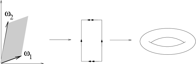
Figure 6: A torus is the quotient of ${\mathbb{C}}$ by a 2-dimensional lattice $\Lambda$.

This second example is actually a prototype for how we will construct Calabi-Yau manifolds. We will embed them in ambient spaces which we know to be complex manifolds and in this way be assured that we inherit a complex structure.

2.2 Equivalences

Given two manifolds $X$ and $Y$, it is important to have a definition which allows us to decide whether they are “different” or “the same”. That is, $X$ and $Y$ might differ only in the particular way they are presented even though fundamentally they are the same manifold. Physically, then, they would be isomorphic and hence we would like to have a framework for classifying the truly distinct possibilities. The notions of homeomorphism, diffeomorphism and biholomorphism provide the mathematics for doing so.

The essential idea is that whether or not $X$ and $Y$ are considered to be “the same” manifold depends upon which of the structures, introduced in the last section, we are considering. Specifically, if $X$ and $Y$ are topological manifolds then we consider them to be the same if they give rise to the same notion of continuity. This is embodied by saying $X$ and $Y$ are homeomorphic if there exists a one-to-one surjective map $\phi:X\rightarrow Y$ (and $\phi^{-1}:Y\rightarrow X$) such that both $\phi$ and $\phi^{-1}$ are continuous (with respect to the topologies on $X$ and $Y$). Such a map $\phi$ allows us to transport the notion of continuity defined by $X$ to that defined by $Y$ and $\phi^{-1}$ does the reverse. Since topological manifolds are characterized by the definition of continuity they provide, $X$ and $Y$ are “the same” — homeomorphic — as topological manifolds. Intuitively, the map $\phi$ allows us to continuously deform $X$ to $Y$.

If we now consider $X$ and $Y$ to be differentiable manifolds, we want to consider them to be equivalent if they not only provide the same notion of continuity, but if they also provide the same notion of differentiability. This is ensured if the maps $\phi$ and $\phi^{-1}$ above are required, in addition, to be differentiable maps. If so, they allow us to freely transport the notion of differentiability defined on $X$ to that on $Y$ and vice versa. If such a $\phi$ exists, $X$ and $Y$ are said to be diffeomorphic.

Finally, if $X$ and $Y$ are complex manifolds, we consider them to be equivalent if there is a map $\phi:X\rightarrow Y$ which in addition to being a diffeomorphism, is also a holomorphic map. That is, when expressed in terms of the complex structures on $X$ and $Y$ respectively, $\phi$ is holomorphic. It is not hard to show that this necessarily implies that $\phi^{-1}$ is holomorphic as well and hence $\phi$ is known as a biholomorphism. Again, such a map allows us to identify the complex structures on $X$ and $Y$ and hence they are isomorphic as complex manifolds.

These definitions do have content in the sense that there are pairs of differentiable manifolds $X$ and $Y$ which are homeomorphic but not diffeomorphic. And, as we shall see, there are complex manifolds $X$ and $Y$ which are diffeomorphic but not biholomorphic. This means that if one simply ignored the fact that $X$ and $Y$ admit local complex coordinates (with holomorphic transition functions), and one only worked in real coordinates, there would be no distinction between $X$ and $Y$. The difference between them only arises from the way in which complex coordinates have been laid down upon them.

Let us see a simple example of this latter phenomenon. Consider the torus $T^{2}$ introduced above as an example of a one-dimensional complex manifold (the superscriipt denotes the real dimension of the torus). To be as concrete as possible, lets consider two choices for the defining lattice $\Lambda$: $(\omega_{1},\omega_{2})=((1,0),(0,1))$ and $(\omega_{1}^{\prime},\omega_{2}^{\prime})=((1,0),(0,2))$. These two tori are drawn in figure 7, where we call the first $X$ and the second $Y$.

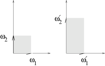
Figure 7: Two diffeomorphic but not biholomorphic tori.

As differentiable manifolds, these two tori are equivalent since the map $\phi$ provides an explicit diffeomorphism:

$$\phi:X\rightarrow Y~{},~{}~{}~{}~{}~{}(y_{1},y_{2})=\phi(x_{1},x_{2})=(x_{1},2x_{2})~{},$$ (2.4)

where $(x_{1},x_{2})$ and $(y_{1},y_{2})$ are local coordinates on $X$ and $Y$. The map $\phi$ clearly meets all of the conditions of a diffeomorphism. However, using local complex coordinates $w=x_{1}+ix_{2}$ and $z=y_{1}+iy_{2}$, we see that

$$(z,\bar{z})=\phi(w,\bar{w})={{3\over 2}}w-{{1\over 2}}\bar{w}$$ (2.5)

and the latter is not a holomorphic function of $w$. Thus, $X$ and $Y$ are diffeomorhpic but not biholomorphic. They are equivalent as differentiable manifolds but not as complex manifolds. In fact, a simple extension of this reasoning shows that for more general choices of $\Lambda$ and $\Lambda^{\prime}$, the tori have the same complex structure if ( but not only if) the ratio $\omega_{2}\over\omega_{1}$ equals $\omega_{2}^{\prime}\over\omega_{1}^{\prime}$. This ratio is usually called $\tau$.

2.3 Tangent Spaces

The tangent space to a manifold $X$ at a point $p$ is the closest flat approximation to $X$ at that point. If the dimension of $X$ is $n$, then the tangent space is an ${\mathbb{R}}^{n}$ which just ‘grazes’ $X$ at $p$, as shown in figure 8. By the familiar definition of tangency from multi-variable calculus, the tangent space at $p$ embodies the “slopes” of $X$ at $p$ — that is, the first order variations along $X$ at $p$. For this reason, a convenient basis for the tangent space of $X$ at $p$ consists of the $n$ linearly independent partial derivative operators:

$$T_{p}X:\Big{\{}{\partial\over\partial x^{1}}\Big{|}_{p},...,{\partial\over\partial x^{n}}\Big{|}_{p}\Big{\}}~{}.$$ (2.6)

A vector $v\in T_{p}X$ can then be expressed as $v=v^{\alpha}{\partial\over\partial x^{\alpha}}|_{p}$. At first sight, it is a bit strange to have partial differential operators as our basis vectors, but a moments thought reveals that this directly captures what a tangent vector really is: a first order motion along $X$ which can be expressed in terms of the translation operators ${\partial\over\partial x^{i}}|_{p}$.

Figure 8: The tangent plane of $X$ at $p$.

Every vector space $V$ has a dual space $V^{\star}$ consisting of real valued linear maps on $V$. Such is the case as well for $V=T_{p}X$ with the dual space being denoted $T^{\star}_{p}X$. A convenient basis for the latter is one which is dual to the basis in (2.6) and is usually denoted by

$$T_{p}^{\star}X:\{dx^{1}|_{p},...,dx^{n}|_{p}\}~{},$$ (2.7)

where, by definition, $dx^{i}:T_{p}X\rightarrow{\mathbb{R}}$ is a linear map with $dx^{i}_{p}({\partial\over\partial x^{j}}|_{p})=\delta^{i}_{j}$. The $dx^{i}$ are called one-forms and we shall often drop the subscript $p$, as the point of reference will be clear from context.

If $X$ is a complex manifold of complex dimension $d=n/2$, there is a notion of the complexified tangent space of $X$, $T_{p}X^{{\mathbb{C}}}$. Concretely, $T_{p}X^{{\mathbb{C}}}$ is the same as the real tangent space $T_{p}X$ except that we allow complex coefficients to be used in the vector space manipulations. This is often denoted by writing $T_{p}X^{{\mathbb{C}}}=T_{p}X\otimes{\mathbb{C}}$. We can still take our basis to be as in (2.6) with an arbitrary vector $v\in T_{p}X^{{\mathbb{C}}}$ being expressed as $v=v^{\alpha}{\partial\over\partial x^{\alpha}}|_{p}$, where the $v^{\alpha}$ can now be complex numbers. In fact, it is convenient to rearrange the basis vectors in (2.6) to more directly reflect the underlying complex structure. Specifically, we take the following linear combinations of basis vectors in (2.6) to be our new basis vectors:

$$T_{p}X^{{\mathbb{C}}}:\Big{\{}\Big{(}{\partial\over\partial x^{1}}+i{\partial\over\partial x^{d+1}}\Big{)}\Big{|}_{p},...,\Big{(}{\partial\over\partial x^{d}}+i{\partial\over\partial x^{2d}}\Big{)}\Big{|}_{p},\Big{(}{\partial\over\partial x^{1}}-i{\partial\over\partial x^{d+1}}\Big{)}\Big{|}_{p},...,\Big{(}{\partial\over\partial x^{d}}-i{\partial\over\partial x^{2d}}\Big{)}\Big{|}_{p}\Big{\}}~{}.$$ (2.8)

In terms of complex coordinates we can write this basis as

$$T_{p}X^{{\mathbb{C}}}:\Big{\{}{\partial\over\partial z^{1}}\Big{|}_{p},...,{\partial\over\partial z^{d}}\Big{|}_{p},{\partial\over\partial{\bar{z}^{1}}}\Big{|}_{p},...,{\partial\over\partial{\bar{z}^{d}}}\Big{|}_{p}\Big{\}}~{}.$$ (2.9)

Notice that from the point of view of real vector spaces, ${\partial\over\partial x^{j}}|_{p}$ and $i{\partial\over\partial x^{j}}|_{p}$ would be considered linearly independent and hence $T_{p}X^{{\mathbb{C}}}$ has real dimension $4d$.

In exact analogy with the real case, we can define the dual to $T_{p}X^{{\mathbb{C}}}$, which we denote by $T_{p}^{\star}X^{{\mathbb{C}}}=T_{p}^{\star}X\otimes{\mathbb{C}}$, with basis

$$T_{p}^{\star}X^{{\mathbb{C}}}:\{dz^{1}|_{p},...,dz^{d}|_{p},d\bar{z}^{1}|_{p},...,d\bar{z}^{d}|_{p}\}~{}.$$ (2.10)

For certain types of complex manifolds $X$ (Calabi-Yau manifolds among these), it is worthwhile to refine the definition of the complexified tangent and cotangent spaces. The refinement we have in mind simply pulls apart the holomorphic and anti-holomorphic directions in each of these two vector spaces. That is, we can write

$$T_{p}X^{{\mathbb{C}}}=T_{p}X^{(1,0)}\oplus T_{p}X^{(0,1)}~{},$$ (2.11)

where $T_{p}X^{(1,0)}$ is the vector space spanned by $\{{\partial\over\partial z^{1}}|_{p},...,{\partial\over\partial z^{d}}|_{p}\}$ and $T_{p}X^{(0,1)}$ is the vector space spanned by $\{{\partial\over\partial\bar{z}^{1}}|_{p},...,{\partial\over\partial\bar{z}^{d}}|_{p}\}$. Similarly, we can write

$$T_{p}^{\star}X^{{\mathbb{C}}}=T_{p}^{\star}X^{(1,0)}\oplus T_{p}^{\star}X^{(0,1)}~{},$$ (2.12)

where $T_{p}^{\star}X^{(1,0)}$ is the vector space spanned by $\{dz^{1}|_{p},...,dz^{d}|_{p}\}$ and $T_{p}^{\star}X^{(0,1)}$ is the vector space spanned by $\{d{\bar{z}^{1}}|_{p},...,d{\bar{z}^{d}}|_{p}\}$. We call $T_{p}X^{(1,0)}$ the holomorphic tangent space; it has complex dimension $d$ and we call $T_{p}^{\star}X^{1,0}$ the holomorphic cotangent space. It also has complex dimension $d$. Their complements are known as the anti-holomorphic tangent and cotangent spaces respectively. The utility of this decomposition depends in part on whether it is respected by parallel translation on $X$; this is a point we shall return to shortly.

2.4 Differential Forms

There is an important generalization of the one-forms we have introduced above. In the context of real manifolds, a one-form is a real valued linear map acting on $T_{p}X$. One generalization of this idea is to consider a $q$-tensor, $\alpha$, which is a real valued multi-linear map from $T_{p}X\times T_{p}X\times...\times T_{p}X$ (with $q$ factors):

$$\alpha(v_{(1)p},...,v_{(q)p})\in{\mathbb{R}}~{}.$$ (2.13)

Multi-linearity here means linear on each factor independently. For our purposes, it proves worthwhile to focus on a more constrained generalization of a one-form called a $q$-form. This is a special type of $q$-tensor which is totally antisymmetric. If $\omega$ is a $q$-form on $X$ at $p$, then

$$\omega(v_{(1)p},...,v_{(q)p})\in{\mathbb{R}}~{},$$ (2.14)

with

$$\alpha(v_{(1)p},v_{(2)p}...,v_{(q)p})=-\alpha(v_{(2)p},v_{(1)p},...,v_{(q)p})$$ (2.15)

and similarly for any other interchange of arguments.

We saw earlier that the $dx^{j}$ form a basis for the the one-forms on $X$ (in a patch with local coordinates given by $(x^{1},...,x^{n})$). A basis for two-tensors can clearly be gotten from considering all $dx^{i}\otimes dx^{j}$, where the notation means that

$$dx^{i}\otimes dx^{j}:T_{p}X\times T_{p}X\rightarrow{\mathbb{R}}$$ (2.16)

in a bilinear fashion according to

$$dx^{i}\otimes dx^{j}({\partial\over\partial x^{k}},{\partial\over\partial x^{l}})=dx^{i}({\partial\over\partial x^{k}})\,dx^{j}({\partial\over\partial x^{l}})=\delta^{i}_{k}\,\delta^{j}_{l}~{}.$$ (2.17)

Now, to get a basis for two-forms, we can simply antisymmetrize the basis for two-tensors by defining

$$dx^{i}\wedge dx^{j}={1\over 2}(dx^{i}\otimes dx^{j}-dx^{j}\otimes dx^{i})~{}.$$ (2.18)

By construction, $dx^{i}\wedge dx^{j}$ satisfies

$$dx^{i}\wedge dx^{j}(v_{(1)},v_{(2)})=-dx^{i}\wedge dx^{j}(v_{(2)},v_{(1)})~{}.$$ (2.19)

It is not hard to show that the $dx^{i}\wedge dx^{j},~{}i<j$ are linearly independent and hence form a basis for two-forms. Any two-form $\omega$, therefore, can be written $\omega=\omega_{ij}dx^{i}\wedge dx^{j}$ for suitable coefficients $\omega_{ij}$. The generalization to a $q$-form is immediate. We construct a basis from all possible

$$dx^{i_{1}}\wedge dx^{i_{2}}\wedge...\wedge dx^{i_{q}}~{},$$ (2.20)

where the latter is defined as

$${{1\over q!}}\sum_{P}{\rm sgn}P\,dx^{i_{P}(1)}\otimes dx^{i_{P}(2)}\otimes...\otimes dx^{i_{P}(q)}~{}.$$ (2.21)

Our notation is that $P$ is a permutation of $1,...,q$ and ${\rm sgn}P$ is $\pm 1$ depending whether the permutation is even or odd. Then, any $q$-form $\omega$ can be written as

$$\omega=\omega_{i_{1}...i_{q}}\,dx^{i_{1}}\wedge dx^{i_{2}}\wedge...\wedge dx^{i_{q}}~{}.$$ (2.22)

The fact that $\omega$ is a totally antisymmetric map is sometimes denoted by $\omega\in\wedge^{q}T^{\star}X$, where $\wedge^{q}$ denotes the $q$-th antisymmetric tensor product.

All of these ideas extend directly to the realm of complex manifolds, together with certain refinements due to the additional structure of having local complex coordinates. If $X$ is a complex manifold of complex dimension $d=n/2$, then we can define a $q$-form as above, except that now we use $\wedge^{q}T^{\star}X^{{\mathbb{C}}}$ instead of $\wedge^{q}T^{\star}X$. As the basis for $T^{\star}X^{{\mathbb{C}}}$ is given in (2.10) we see that by suitable rearrangement of indices we can write a $q$-form $\omega$ as

$$\omega=\omega_{i_{1}...i_{q}}\,dt^{i_{1}}\wedge dt^{i_{2}}\wedge...\wedge dt^{i_{q}}~{},$$ (2.23)

where each $dt^{j}$ is an element of the basis in (2.10). Any summand in (2.23) can be labelled by the number $r$ of holomorphic one-forms it contains and by the number $s=q-r$ of anti-holomorphic one-forms it contains. By suitable rearrangement of indices we can then write

$$\omega=\sum_{r}\,\omega_{i_{1}...i_{r}\bar{\jmath}_{1}...\bar{\jmath}_{q-r}}\,dz^{i_{1}}\wedge dz^{i_{2}}\wedge...\wedge dz^{i_{r}}\wedge d\overline{z}^{\bar{\jmath}_{1}}\wedge d\overline{z}^{\bar{\jmath}_{2}}\wedge...\wedge d\overline{z}^{\bar{\jmath}_{q-r}}~{}.$$ (2.24)

Each summand on the right hand side is said to belong to $\Omega^{r,s}(X)$, the space of antisymmetric tensors with $r$ holomorphic and $s$ anti-holomorphic indices. In this notation, then, $\Omega^{r,s}(X)=\wedge^{r}T^{\star(1,0)}X\otimes\wedge^{s}T^{\star(0,1)}X$.

2.5 Cohomology and Harmonic Analysis — Part I

There is a natural differentiation operation that takes a $q$-form $\omega$ on a differentiable manifold $X$ to a $(q+1)$-form on $X$. That is, there is a map

$$d:\bigwedge^{q}T^{\star}X\rightarrow\bigwedge^{q+1}T^{\star}X~{}.$$ (2.25)

Explicitly, in local coordinates this map $d$, known as exterior differentiation, is given by

$$d:\omega\rightarrow d\omega={\partial\omega_{i_{1}...i_{q}}\over\partial x^{i_{q+1}}}\,dx^{i_{q+1}}\wedge dx^{i_{1}}\wedge dx^{i_{2}}\wedge...\wedge dx^{i_{q}}~{}.$$ (2.26)

By construction, the right hand side is a $(q+1)$-form on $X$. We will return to study the properties of forms and exterior differentiation. First, though, we note that if $X$ is a complex manifold, there is a refinement of exterior differentiation which will prove to be of central concern.

Namely, let $\omega^{r,s}=\omega_{i_{1}...i_{r}\bar{\jmath}_{1}...\bar{\jmath}_{s}}dz^{i_{1}}\wedge...\wedge dz^{i_{r}}\wedge d\bar{z}^{\bar{\jmath}_{1}}\wedge...\wedge d\bar{z}^{\bar{\jmath}_{s}}$ be in $\Omega^{r,s}(X)$. Then, since $\omega^{r,s}$ can certainly be thought of as a real $(r+s)$-form on $X$, $d\omega^{r,s}$ is an $(r+s+1)$-form on $X$. This form may be decomposed using the complex structure of $X$ into an element of $\Omega^{r+1,s}(X)\oplus\Omega^{r,s+1}(X)$. Explicitly,

$$d\omega^{r,s}\!\!\!\! = \!\!\!\!{\partial\omega_{i_{1}...i_{r}\bar{\jmath}_{1}...\bar{\jmath}_{s}}\over\partial z^{i_{r+1}}}dz^{i_{r+1}}\wedge dz^{i_{1}}\wedge dz^{i_{2}}\wedge...\wedge dz^{i_{r}}\wedge d\bar{z}^{\bar{\jmath}_{1}}\wedge d\bar{z}^{\bar{\jmath}_{2}}\wedge...\wedge d\bar{z}^{\bar{\jmath}_{s}}$$

$$+ \!\!\!\!{\partial\omega_{i_{1}...i_{r}\bar{\jmath}_{1}...\bar{\jmath}_{s}}\over\partial\bar{z}^{i_{s+1}}}dz^{i_{1}}\wedge dz^{i_{2}}\wedge...\wedge dz^{i_{r}}\wedge d{\bar{z}^{\bar{\jmath}_{s}+1}}\wedge d{\bar{z}^{\bar{\jmath}_{1}}}\wedge d\bar{z}^{\bar{\jmath}_{2}}\wedge...\wedge d\bar{z}^{\bar{\jmath}_{s}}~{}.$$

This equation is often summarized by writing

$$d\omega^{r,s}=\partial\omega^{r,s}+\bar{\partial}\omega^{r,s}~{},$$ (2.27)

where we are decomposing the real exterior differentiation operator $d$ as $d=\partial+\bar{\partial}$, the latter two being exterior differentiation in the holomorphic and anti-holomorphic directions respectively.

There are many uses of exterior differentiation; we note one here. The antisymmetry involved in exterior differentiation ensures that $d(d\alpha)=0$ for any form $\alpha$. That is, $d^{2}=0$. Now, if it so happens that $\omega$ is a $q$-form for which $d\omega=0$ — such an $\omega$ is called closed — there are then two possibilities. Either $\omega$ is exact which means that it can be written as $d\beta$ for a $(q-1)$-form $\beta$, in which case $d\omega=0$ follows from the stated property of $d^{2}=0$, or $\omega$ cannot be so expressed. Those $\omega$ which are closed but not exact provide non-trivial solutions to the equation $d\omega=0$ which motivates the following defintion.

This $q$-th DeRham cohomology group $H^{q}_{d}(X)$ on a real differentiable manifold $X$ is the quotient space

$$H^{q}_{d}(X,{\mathbb{R}})={{\{\omega|d\omega=0\}\over\{\alpha|\alpha=d\beta\}}}~{},$$ (2.28)

where $\omega$ and $\alpha$ are $q$-forms.

Again, if $X$ is a complex manifold, there is a refinement of DeRham cohomology into Dolbeault cohomology in which rather than using the $d$ operator, we make use of the $\bar{\partial}$ operator. Since $\bar{\partial}^{2}=0$, it makes sense to form the $(r,s)$-th Dolbeault cohomology group on $X$ via

$$H^{r,s}_{\bar{\partial}}(X,{\mathbb{C}})={{\{\omega^{r,s}|\bar{\partial}\omega^{r,s}=0\}\over\{\alpha^{r,s}|\alpha^{r,s}=\bar{\partial}\beta^{r,s-1}\}}}~{}.$$ (2.29)

This could also be formulated using $\partial$.

The cohomology groups of $X$ probe important fundamental information about its geometrical structure, and will play a central role in our physical analysis.

2.6 Metrics: Hermitian and Kähler Manifolds

A metric $g$ on a real differentiable manifold $X$ is a symmetric positive map

$$g:T_{p}X\times T_{p}X\rightarrow{\mathbb{R}}~{}.$$ (2.30)

In local coordinates, $g$ can be written as $g=g_{ij}\,dx^{i}\otimes dx^{j}$ where the coeffecients satisfy $g_{ij}=g_{ji}$. By measuring lengths of tangent vectors according to $g(v_{p},v_{p})$, the metric can be used to measure distances on $X$.

If $X$ is a complex manifold, there is a natural extension of the metric $g$ to a map

$$g:T_{p}X^{{\mathbb{C}}}\times T_{p}X^{{\mathbb{C}}}\rightarrow{\mathbb{C}}$$ (2.31)

defined in the following way. Let $r,s,u,v$ be four vectors in $T_{p}X$. Using them, we can construct, for example, two vectors $w_{(1)}=r+is$ and $w_{(2)}=u+iv$ which lie in $T_{p}X^{{\mathbb{C}}}$. Then, we evaluate $g$ on $w_{(1)}$ and $w_{(2)}$ by linearity:

$$g(w_{(1)},w_{(2)})=g(r+is,u+iv)=g(r,u)-g(s,v)+i\,[g(r,v)+g(s,u)]~{}.$$ (2.32)

We can define components of this extension of the original metric (which we have called by the same symbol) with respect to complex coordinates in the usual way: $g_{ij}=g({{\partial\over\partial z^{i}}},{{\partial\over\partial z^{j}}})$, $g_{i\bar{\jmath}}=g({{\partial\over\partial z^{i}}},{{\partial\over\partial\bar{z}^{\bar{\jmath}}}})$ and so forth. The reality of our original metric $g$ and its symmetry implies that in complex coordinates we have $g_{ij}=g_{ji}$, $g_{i\bar{\jmath}}=g_{\bar{\jmath}i}$ and $\overline{g_{ij}}=g_{\bar{\imath}\bar{\jmath}}$, $\overline{g_{i\bar{\jmath}}}=g_{\bar{\imath}j}$.

So far our discussion is completely general. We started with a metric tensor on $X$ viewed as a real differentiable manifold and noted that it can be directly extended to act on the complexified tangent space of $X$ when the latter is a complex manifold. Now we consider two additional restrictions that prove to be quite useful.

The first is the notion of a hermitian metric on a complex manifold $X$. In local coordinates, a metric $g$ is Hermitian if $g_{ij}=g_{\bar{i}\bar{j}}=0$. In this case, only the mixed type components of $g$ are nonzero and hence it can be written as

$$g=g_{i\bar{\jmath}}\,dz^{i}\otimes d{\bar{z}^{\bar{\jmath}}}+g_{\bar{\imath}j}\,d{\bar{z}^{\bar{\imath}}}\otimes dz^{j}~{}.$$ (2.33)

With a little bit of algebra one can work out the constraint this implies for the original metric written in real coordinates. (Abstractly, for those who are a bit more familiar with these ideas, if ${\cal J}$ is a complex structure acting on the real tangent space $T_{p}X$, i.e. ${\cal J}:T_{p}X\rightarrow T_{p}X$ with ${\cal J}^{2}=-I$, then the hermiticity condition on $g$ is $g({\cal J}v_{(1)},{\cal J}v_{(2)})=g(v_{(1)},v_{(2)})$.)

The second is the notion of kählerity, which will define the third term in the definition of a Calabi-Yau manifold. Given a hermitian metric $g$ on $X$, we can build a form in $\Omega^{1,1}(X)$ — that is, a form of type $(1,1)$ in the following way:

$$J=ig_{i\bar{\jmath}}\,dz^{i}\otimes d{\bar{z}^{\bar{\jmath}}}-ig_{\bar{\jmath}i}\,d{\bar{z}^{\bar{\jmath}}}\otimes dz^{i}~{}.$$ (2.34)

By the symmetry of $g$, we can write this as

$$J=ig_{i\bar{\jmath}}\,dz^{i}\wedge d{\bar{z}^{j}}~{}.$$ (2.35)

Now, if $J$ is closed, that is, if $dJ=0$, then $J$ is called a Kähler form and $X$ is called a Kähler manifold. At first sight, this kählerity condition might not seem too restrictive. However, it leads to remarkable simplifications in the resulting differential geometry on $X$, as we indicate in the next section.

2.7 Kähler Differential Geometry

In local coordinates, the fact that $dJ=0$ for a Kähler manifold implies

$$dJ=(\partial+\bar{\partial})ig_{i\bar{\jmath}}\,dz^{i}\wedge d\bar{z}^{\bar{\jmath}}=0~{}.$$ (2.36)

This implies that

$${{\partial g_{i\bar{\jmath}}\over\partial z^{l}}}={{\partial g_{l\bar{\jmath}}\over\partial z^{i}}}$$ (2.37)

and similary with $z$ and $\bar{z}$ interchanged. From this we see that locally we can express $g_{i\bar{\jmath}}$ as

$$g_{i\bar{\jmath}}={\partial^{2}K\over\partial z^{i}\partial\bar{z}^{\bar{\jmath}}}~{}.$$ (2.38)

That is, $J=i\partial\bar{\partial}K$, where $K$ is a locally defined function in the patch whose local coordinates we are using, which is known as the Kähler potential.

Given a metric on $X$, we can calculate the Levi-Civita connection as in standard general relativity from the formula

$$\Gamma^{i}_{jk}={{1\over 2}}g^{il}({{\partial g_{lk}\over\partial x^{j}}}+{{\partial g_{lj}\over\partial x^{k}}}-{{\partial g_{jk}\over\partial x^{l}}})~{}.$$ (2.39)

Now, if $J$ on $X$ is a Kähler form, the conditions (2.37) imply that there are numerous cancellations in (2.39). In fact, the only nonzero Christoffel symbols in complex coordinates are those of the form $\Gamma^{l}_{jk}$ and $\Gamma^{\bar{l}}_{\bar{\jmath}\bar{k}}$, with all indices holomorphic or anti-holomorphic. Specifically,

$$\Gamma^{l}_{jk}=g^{l\bar{s}}\,{{\partial g_{k\bar{s}}\over\partial z^{j}}}$$ (2.40)

and

$$\Gamma^{\bar{l}}_{\bar{\jmath}\bar{k}}=g^{\bar{l}s}\,{{\partial g_{\bar{k}s}\over\partial{\bar{z}^{\bar{\jmath}}}}}~{}.$$ (2.41)

The curvature tensor also greatly simplifies. The only non-zero components of the Riemann tensor, when written in complex coordinates, have the form $R_{i\bar{\jmath}k\bar{l}}$ (up to index permutations consistent with symmetries of the curvature tensor). And we have

$$R_{i\bar{\jmath}k\bar{l}}=g_{i\bar{s}}\,{{\partial\Gamma^{\bar{s}}_{\bar{\jmath}\bar{l}}\over\partial z^{k}}}~{},$$ (2.42)

as well as the Ricci tensor

$$R_{\bar{\imath}j}=R^{\bar{k}}_{~{}\bar{\imath}\bar{k}j}=-{{\partial\Gamma^{\bar{k}}_{\bar{\imath}\bar{k}}\over\partial z^{j}}}~{}.$$ (2.43)

2.8 Holonomy

Using the above results, we can now describe the final element in the definition of a Calabi-Yau manifold. First, let $X$ be a real differentiable manifold of real dimension $n$, and let $v\in T_{p}X$. Assuming that $X$ is equipped with a metric $g$ and the associated Levi-Civita connection $\Gamma$, we can imagine parallel transporting $v$ along a curve $C$ in $X$ which begins and ends at $p$. After the journey around the curve, the vector $v$ will generally not return to its original orientation in $T_{p}X$. Rather, if $X$ is not flat, $v$ will return to $p$ pointing in another direction, say $v^{\prime}$. (Since we are using the Levi-Civita connection for parallel transport, the length of $v$ will not change during this process.) If $X$ is orientable, the vectors $v$ and $v^{\prime}$ will be related by an $SO(n)$ transformation $A_{C}$, where the subscript reminds us of the curve we have moved around. That is

$$v^{\prime}=A_{C}v~{}.$$ (2.44)

Now consider all possible closed curves in $X$ which pass through $p$, and repeat the above procedure. This will yield a collection of $SO(n)$ matrices $A_{C_{1}},A_{C_{2}},A_{C_{3}},...$, one for each curve. Notice that if we traverse a curve $C$ which is the curve $C_{i}$ followed by the curve $C_{j}$, the associated matrix will be $A_{C_{j}}A_{C_{i}}$ and that if we traverse the curve $C_{j}$ in reverse, the associated matrix will be $A_{C_{j}}^{-1}$. Thus, the collection of matrices generated in this manner form a group — namely, some subgroup of $SO(n)$. Let us now take this one step further by following the same procedure at all points $p$ on $X$. Similar reasoning to that just used ensures that this collection of matrices also forms a group. This group describing how vectors change upon parallel translation around loops on $X$ is called the holonomy of $X$.

For a “generic” (orientable) differentiable manifold $X$, the holonomy group will fill out all of $SO(n)$, but when $X$ meets certain other requirements, the holonomy group can be a proper subgroup. The simplest example of this is when $X$ is flat. In this case, the orientation of parallel transported vectors does not change and hence the holonomy group consists solely of the identity element. In between these two extremes — all of $SO(n)$ and the identity — a number of other things can happen. We will be interested in two of these.

First, if $X$ is a complex Kähler manifold, we have seen above a number of simplifications which occur in the differential geometry associated to $X$. In particular, the Levi-Civita connection, as seen in (2.40) and (2.41), only has nonzero components for indices of the same type. As the connection controls parallel transport, this implies that if $v$ is expressed in complex coordinates as

$$v=v^{j}{{\partial\over\partial z^{j}}}+v^{\bar{\jmath}}{\partial\over\partial\bar{z}^{\bar{\jmath}}}~{},$$ (2.45)

then the holomorphic components $v^{j}$ and anti-holomorphic components $v^{\bar{\jmath}}$ do not mix together. In other words, the decomposition at a point $p$ of $T_{p}X^{{\mathbb{C}}}=T_{p}^{(1,0)}X\oplus T_{p}^{(0,1)}X$ is unaffected by parallel translation away from $p$. The individual factors in the direct sum do not mix.

In terms of the holonomy group, this implies that the holonomy matrices can consistently be written in terms of their action on the holomorphic or anti-holomorphic basis elements and hence lie in a $U(d)$ subgroup of $SO(n)$ (where, as before, $d=n/2$).

The second special case are those complex Kähler manifolds whose holonomy group is even further restricted to lie in $SU(d)$. Although equally consistent as string compactifications, we will typically not discuss $X$ whose holonomy is a proper subgroup of $SU(d)$. Hence, we shall take Calabi-Yau to mean holonomy which fills out $SU(d)$. In essence, as we shall discuss shortly, having holonomy $SU(d)$ means that the $U(1)$ part of the Levi-Civita connection $\Gamma$ vanishes. This can be phrased as a topological restriction on $X$ which will greatly aid in the construction of examples.

2.9 Cohomology, Harmonic Analysis — Part II

We discussed previously the operation of exterior differentiation $d$ which takes a differential $p$-form to a differential $(p+1)$-form. If the manifold $X$ on which these forms are defined has a Riemannian metric, then the operation $d$ has an adjoint $d^{\dagger}$, which maps $p$-forms to $(p-1)$-forms, defined in the following way:

$$d^{\dagger}:\omega\rightarrow d^{\dagger}\omega=-{1\over(p-1)!}\,\omega^{\mu}_{~{}\mu_{1}\dots\mu_{p-1};\mu}\,dx^{\mu_{1}}\wedge\dots\wedge dx^{\mu_{p-1}}~{},$$ (2.46)

where $\omega^{\mu}_{~{}\nu\dots;\rho}$ denotes the covariant derivative of $\omega^{\mu}_{~{}\nu\dots}~{}.$

To understand the meaning of this operation in greater detail, it is necessary to introduce the notion of the Hodge star operation $\star$, which is important in its own right. This operator maps a $p$-form on a $n$-dimensional differentiable manifold with metric $g$ to an $(n-p)$-form. Explicitly,

$$\omega\rightarrow\star\omega={1\over(n-p)!p!}\,\epsilon_{i_{1},...,i_{n}}\,\sqrt{|{\rm det}g|}\,g^{i_{1}j_{1}}...g^{i_{p}j_{p}}\,\omega_{j_{1}...j_{p}}\,dx^{i_{p+1}}\wedge...\wedge dx^{i_{n}}~{}.$$ (2.47)

This map has the virtue of being bijective and coordinate independent.

Notice now that the composition $\star d\star$ maps a $p$-form first to an $(n-p)$-form, then to a $(n-p+1)$-form and finally to a $(p-1)$-form. In fact,

$$d^{\dagger}=(-1)^{np+n+1}\star d\star~{}.$$ (2.48)

From a more abstract point of view, the Hodge star operator gives us an inner product on $p$-forms via

$$\langle\omega,\omega^{\prime}\rangle=\int_{X}\omega\wedge\star\omega^{\prime}~{}.$$ (2.49)

We can then define the adjoint of $d$ from the requirment that if $\beta$ is a $(p-1)$-form and $\omega$ is a $p$-form, then

$$\langle\omega,d\beta\rangle=\langle d^{\dagger}\omega,\beta\rangle~{}.$$ (2.50)

When expressed in local coordinates, we obtain (2.46).

There are numerous uses of $d$ and $d^{\dagger}$ in both mathematics and physics. Here we focus on one — the Hodge decomposition theorem — which states that any $p$-form on $X$ can be uniquely written as

$$\omega=d\beta+d^{\dagger}\gamma+\omega^{\prime}~{},$$ (2.51)

where $\beta$ is a $(p-1)$-form, $\gamma$ is a $(p+1)$-form, and $\omega^{\prime}$ is a harmonic $p$-form. By definition, a harmonic form is one that is annihilated by $\Delta=d^{\dagger}d+dd^{\dagger}$, which is the Laplacian acting on $p$-forms. It is easy to check by writing $\Delta$ in local coordinates, that it is the curved space generalization of the ordinary Laplacian on ${\mathbb{R}}^{n}$.

In particular, if $\omega$ is closed then it is not hard to show that $\gamma$ vanishes and hence we can write

$$\omega=d\beta+\omega^{\prime}~{}.$$ (2.52)

From our earlier discussion of cohomology, we now recognize $\omega-d\beta$ as an element of $H^{p}(X,{\mathbb{R}})$ and hence we learn that there is a unique harmonic $p$-form representative in each cohomology class of $H^{p}(X,{\mathbb{R}})$.

As in the previous sections, if $X$ is a complex manifold and $\omega^{r,s}$ is an $(r,s)$-form, the complex Hodge decomposition allows us to write

$$\omega^{r,s}=\overline{\partial}\alpha^{r,s-1}+\overline{\partial}^{\dagger}\beta^{r,s+1}+\omega^{\prime r,s}~{},$$ (2.53)

where $\omega^{\prime r,s}$ is harmonic with respect to the Laplacian $\Delta_{\bar{\partial}}=\overline{\partial}^{\dagger}\overline{\partial}+\overline{\partial}\overline{\partial}^{\dagger}$.

As in the real case, if $\omega^{r,s}$ is $\overline{\partial}$ closed, then this decomposition gives us a unique $\Delta_{\bar{\partial}}$ harmonic representative for each class in $H^{r,s}_{\bar{\partial}}(X,{\mathbb{C}})$.

In the special case in which $X$ is a Kähler manifold, it is straightforward to show that all of the Laplacians built from $d$, $\overline{\partial}$ and $\partial$, namely $\Delta$, $\Delta_{\overline{\partial}}$ and $\Delta_{\partial}$ are related by

$$\Delta=2\Delta_{\overline{\partial}}=2\Delta_{\partial}~{}.$$ (2.54)

In this case, then, the harmonic forms with respect to each operator are the same.

We define $h^{r,s}_{X}$ to be the (complex) dimension of $H^{r,s}_{\bar{\partial}}(X,{\mathbb{C}})$ which is the same as the dimension of the vector space of harmonic $(r,s)$-forms on $X$. The Hodge star operator, with the obvious extension into the complex realm, ensures

$$h^{r,s}_{X}=h^{m-r,m-s}_{X}~{}.$$ (2.55)

Using complex conjugation and Kählerity, we also have

$$h^{r,s}_{X}=h^{s,r}_{X}~{}.$$ (2.56)

Kählerity also ensures the following relation between $d$ and $\overline{\partial}$ cohomology:

$$H^{p}_{d}(X)=\bigoplus_{r+s=p}\,H_{\overline{\partial}}^{r,s}(X).$$ (2.57)

2.10 Examples of Kähler Manifolds

The simplest example of a Kähler manifold is ${\mathbb{C}}^{m}$. We can write a Kähler form associated to the usual Euclidean metric written in complex coordinates $g=\sum_{j}dz^{j}\otimes d{\overline{z}}^{j}$ as $J={{i\over 2}}\sum_{j}dz^{j}\wedge d{\overline{z}}^{j}$. Clearly $J$ is closed.

The next simplest examples of Kähler manifolds are Riemann surfaces. These are orientable complex manifolds of complex dimension 1. They are Kähler since every two-form is closed (as the real dimension being two cannot support forms of higher degree).

Of most use in our subsequent discussions, are the examples of ordinary and weighted complex projective spaces. Let us define these.

The ordinary complex projective $n$-space, ${\mathbb{C}}P^{n}$, is defined by introducing $n+1$ homogeneous complex coordinates $z_{1},...,z_{n+1}$ not all of them simultaneously zero with an equivalence relation stating that points labelled by $(z_{1},...,z_{n+1})$ are identified with points labelled by $(\lambda z_{1},...,\lambda z_{n+1})$ for any complex number $\lambda$. In reality, the $z_{i}$ are therefore not local coordinates in the technical sense. Rather, in the $j$-th patch, defined by $z^{j}\neq 0$, we can choose $\lambda=1/z^{j}$ and use local coordinates

$$(\xi_{(j)}^{1},\dots,\xi_{(j)}^{n})=({{z_{1}\over z_{j}}},...,{{z_{j-1}\over z_{j}}},{{z_{j+1}\over z_{j}}},\dots,{{z_{n+1}\over z_{j}}})~{}.$$

We can see that ${\mathbb{C}}P^{n}$ is Kähler by defining $K_{j}$ in the $j$-th patch to be $K_{j}=\sum|{{z^{i}\over z_{j}}}|^{2}$. Then $J=\partial\overline{\partial}K_{j}$ is a globally defined closed 2-form class on $X$. To see this, since we defined $J$ patch by patch, one must only check that the differences in patch overlaps are exact. The metric associated to $J$ is called the Fubini-Study metric.

For later use we point out that by suitable choice of $|\lambda|$, we can always choose our representatives from the equivalence class of homogeneous coordinates to satisfy

$$\sum_{i}|z_{i}|^{2}=r$$ (2.58)

for some arbitrarily chosen positive real number $r$. This “fixes” part of the ${\mathbb{C}}^{*}$ equivalence relation defining the projective space. The rest — associated with the phase of $\lambda$ — is implemented by identifying

$$(z_{1},...,z_{n+1})\sim(e^{i\theta}z_{1},...,e^{i\theta}z_{n+1}).$$ (2.59)

The weighted projective space $W{\mathbb{C}}P^{n}(\omega_{1}$, $\omega_{2}$, $...$, $\omega_{n+1})$ is a simple generalization of ordinary projective space in which the homogeneous coordinate identification is

$$(z_{1},...,z_{n+1})\sim(\lambda^{\omega_{1}}z_{1},...,\lambda^{\omega_{n+1}}z_{n+1})~{}.$$ (2.60)

It is again not hard to show that this space is Kähler. One complication is that $W{\mathbb{C}}P^{n}(\omega_{1},...,\omega_{n+1})$ is not generally smooth because non-trivial fixed points under the coordinate identification lead to singularities. Specifically, if the weights $(\omega_{1},...,\omega_{n+1})$ are not all relatively prime, then there will be non-trivial values of $\lambda$ so that $\lambda^{\omega_{i}}=\lambda^{\omega_{j}}=1$ for some $i\neq j$. By setting to zero all of the homogeneous coordinates whose weights do not satisfy this equation, we will find a subspace of the weighted projective space which is singular due to its being a fixed point set of the coordinate identification.

In the rest of the lectures, we will be interested in compact Kähler manifolds constructed as subspaces of larger complex manifolds. We thus explain some notions and results in this direction.

An analytic submanifold $N$ of the complex manifold $M$ is defined by a set of analytic equations

$$N=\{p\in M~{}:~{}f^{\alpha}(p)=0,~{}\alpha=1,\dots,m\leq n\}~{},$$ (2.61)

such that

$${\rm rank}[{\partial f^{\alpha}\over\partial z^{j}}\Big{|}_{p}]$$ (2.62)

where $z^{j},~{}j=1,\dots,n$ are the coordinates on $M$, is independent of the point $p\in M$ and equals $m$. When $f^{\alpha}$ are polynomials, we call $N$ an algebraic variety in $M$.

Then by letting

$$w^{\alpha}(p) \equiv f^{\alpha}(p)~{},~{}~{}~{}~{}~{}\alpha=1,\dots,m~{},$$ (2.63)

$$w^{i}(p) \equiv z^{i}(p)~{},~{}~{}~{}~{}~{}i=m+1,\dots,n~{},$$ (2.64)

we have a system of local coordinates such that $N$ is defined by

$$w^{1}(p)=w^{2}(p)=\dots=w^{m}(p)=0~{}.$$

Then $\zeta^{i}(p)=w^{i+m}(p),~{}i=1,\dots,n-m$ are the local coordinates of $N$; therefore, the submanifold has (complex) dimension $n-m$. (This construction of local coordinates will be explained in the example below).

Now, let $M={\mathbb{C}}^{n}$. Under what conditions is $N$ a compact (analytic) submanifold? To answer this question, we recall the maximum modulus theorem from complex analysis. According to this theorem, an analytic function on a domain $D\subset{\mathbb{C}}$ cannot have an extremum on $D$ unless it is a constant. This theorem can be extended to the case of ${\mathbb{C}}^{n}$.

If $N\subset{\mathbb{C}}^{n}$ is a compact submanifold of ${\mathbb{C}}^{n}$, the functions $f^{\alpha}(\zeta)$ are analytic functions of $\zeta$ on $M$ and since $N$ is compact each $f^{i}$ much be constant. We thus arrive at the conclusion that any compact submanifold of ${\mathbb{C}}^{n}$ has to be a point!

With the result of the last pragraph at hand, we are led to examine the construction of compact submanifolds within other complex manifolds. A natural next choice is ${\mathbb{C}}P^{n}$. In fact, ${\mathbb{C}}P^{n}$ is compact and all its complex submanifolds are compact. There is a famous theorem due to Chow:

Theorem 1 (Chow)

Any submanifold of ${\mathbb{C}}P^{n}$ can be realized as the zero locus of a finite number of homogeneous polynomial equations.

A well studied example of the above discussion, that will show up in many places in the present lectures, is the set of points in ${\mathbb{C}}P^{4}$ given by the locus of zeros of the equation

$$\sum_{i=1}^{5}\,(z_{i})^{5}=0~{}.$$ (2.65)

Let us denote it by $P$ and explain how one places local coordinates upon it. Using the patches $U_{j}=\{z\in{\mathbb{C}}^{5}-{0},z_{j}\neq 0\}$ and the corresponding coordinates $\xi^{i}_{(j)},~{}j=1,2,3,4$ for ${\mathbb{C}}P^{4}$ defined above, the equation (2.65) can be rewritten in the form:

$$1+\sum_{i=1}^{4}\,(\xi_{(j)}^{i})^{5}=0~{},$$ (2.66)

on the patch $U_{j}$.

We now concentrate on the patch $U_{1}$ of ${\mathbb{C}}P^{4}$. Here, we make the following holomorphic change of coordinates

$$\eta^{1} = 1+\sum_{i=1}^{4}\,(\xi_{(1)}^{i})^{5}~{},$$

$$\eta^{2} = \xi_{(1)}^{2}~{},$$

$$\eta^{3} = \xi_{(1)}^{3}~{},$$

$$\eta^{4} = \xi_{(1)}^{4}~{}.$$

The new variables will be good coordinates if the Jacobian

$${\partial(\eta)\over\partial(\xi)}=5\,(\xi_{(1)}^{1})^{4}=5\,\left({z_{2}\over z_{1}}\right)^{4}$$ (2.67)

does not vanish. Therefore, as long as $z_{2}\neq 0$, the part of $P$ found in $U_{1}$ is given by $\eta^{1}=0$. We have thus constructed a patch $V_{1}=P\cap U_{1}$ (actually is $P\cap U_{1}\cap U_{2}$ since $z_{2}\neq 0$)

$$V_{1}=\{(\eta^{1},\eta^{2},\eta^{3},\eta^{4})\in{\mathbb{C}}^{4}~{},~{}\eta^{1}=0\}$$

on $P$ and a local coordinate system

$$\zeta^{1}_{(1)}=\eta^{2}~{},~{}~{}~{}\zeta^{2}_{(1)}=\eta^{3}~{},~{}~{}~{}\zeta^{3}_{(1)}=\eta^{4}~{}.$$

When $z_{2}=0$, the transformation $\xi\rightarrow\eta$ is not well defined; in this case we introduce another transformation:

$$\eta^{1} = \xi_{(1)}^{2}~{},$$

$$\eta^{2} = 1+\sum_{i=1}^{4}\,(\xi_{(1)}^{i})^{5}~{},$$

$$\eta^{3} = \xi_{(1)}^{3}~{},$$

$$\eta^{4} = \xi_{(1)}^{4}~{}.$$

This transformation is well defined if $z_{3}\neq 0$. Continuing in this manner, an atlas for $P$ can be constructed.

2.11 Calabi-Yau Manifolds

We have now defined all of the mathematical ingredients to understand and study Calabi-Yau manifolds. Just to formalize things we write

Definition 1

A Calabi-Yau manifold is a compact, complex, Kähler manifold which has $SU(d)$ holonomy.

For the most part we shall study the case of $d=3$. An equivalent statement is that a Calabi-Yau manifold admits a Ricci-flat metric:

$$R_{i\bar{\jmath}}=-{{\partial\over\partial{\overline{z}^{\bar{\jmath}}}}}\Gamma_{ik}^{k}=0~{}.$$

It is not hard to show that the vanishing of the $U(1)$ part of the connection, effectively its trace, which ensures that the holonomy lies in $SU(d)$ is tantamount to having a Ricci-flat metric. We will generally take Calabi-Yau to mean holonomy being precisely $SU(d)$ as mentioned in the definition.

An important theorem, both from the abstract and practical perspectives, is that due to Yau who proved Calabi’s conjecture that a complex Kähler manifold of vanishing first Chern class admits a Ricci-flat metric. We will not cover Chern classes in these notes in any detail; for this the reader can consult, for instance, [69]. Briefly, though, the Chern classes of $X$ probe basic topological properties of $X$. Specifically, the $k$-th Chern class $c_{k}(X)$ is an element of $H^{k}_{d}(X)$ defined from the expansion

$$c(X)=1+\sum_{j}c_{j}(X)=\det(1+{\cal R})=1+{\rm tr}{\cal R}+{\rm tr}({\cal R}\wedge{\cal R}-2({\rm tr}{\cal R})^{2})+...~{},$$ (2.68)

where ${\cal R}$ is the matrix valued curvature 2-form

$${\cal R}=R^{k}_{~{}li\bar{\jmath}}\,dz^{i}\wedge d\bar{z}^{\bar{\jmath}}~{}.$$

We should point out that the curvature tensor $R$ is really being thought of as the curvature tensor of the tangent bundle $T_{X}$ of $X$, with the matrix indices being those in the fiber direction. Thus, often $c(X)$ is also written as $c(T_{X})$.

Rather remarkably, although constructed from the local curvature tensor, the Chern classes only depend on far more crude topological properties of $X$. We see directly that if $X$ has vanishing Ricci tensor, then the first Chern class, being the trace of the curvature 2-form, vanishes. Yau’s theorem goes in the other direction and shows that if the first Chern class vanishes (as a cohomology class in $H^{2}_{d}(X)$) then $X$ admits a Ricci-flat metric. More precisely,

Theorem 2 (Yau)

If X is a complex Kähler manifold with vanishing first Chern class and with Kähler form $J$, then there exists a unique Ricci-flat metric on $X$ whose Kähler from $J^{\prime}$ is in the same cohomology class as $J$.

The utility of this theorem is that it is generally quite hard to directly determine whether or not $X$ admits a Ricci-flat metric $g$. In fact, no explicit Ricci-flat metrics are known on any Calabi- Yau manifolds. On the other hand, it is a simple matter to compute the first Chern class of $X$, and, in particular, to find examples with vanishing first Chern class. Yau’s theorem then ensures the existence of a Ricci-flat metric.

In our subsequent discussions, we will need to know various things regarding the cohomology of Calabi-Yau manifolds. There are a number of simplifications which occur relative to the general Kähler manifold. In particular, since the holonomy is $SU(d)$, it can be shown that $h^{0,s}=h^{s,0}=0$ for $1<s<d$ and that $h^{0,d}=h^{d,0}=1$. The latter is a holomorphic, nowhere vanishing differential form of type $(d,0)$ on the Calabi-Yau, usually referred to as $\Omega$. Using the fact that the space $X$ is connected we also have $h^{0,0}=1$. We therefore have the following form for the Hodge numbers (arranged in the so-called Hodge diamond) for $d=1,2,3$:

				$h^{0,0}$								1
$d=1$			$h^{1,0}$		$h^{0,1}$			=			1		1
				$h^{1,1}$								1
				$h^{0,0}$								1
			$h^{1,0}$		$h^{0,1}$						0		0
$d=2$		$h^{2,0}$		$h^{1,1}$		$h^{0,2}$		=		1		20		1
			$h^{2,1}$		$h^{1,2}$						0		0
				$h^{2,2}$								1
				$h^{0,0}$								1
			$h^{1,0}$		$h^{0,1}$						0		0
		$h^{2,0}$		$h^{1,1}$		$h^{0,2}$				0		$h^{1,1}$		0
$d=3$	$h^{3,0}$		$h^{2,1}$		$h^{1,2}$		$h^{0,3}$	=	1		$h^{2,1}$		$h^{2,1}$		1
		$h^{3,1}$		$h^{2,2}$		$h^{1,3}$				0		$h^{1,1}$		0
			$h^{3,2}$		$h^{2,3}$						0		0
				$h^{3,3}$								1

Notice that in the two-dimensional case we have explicitly filled in $h^{1,1}=20$. We will derive this shortly. The key distinction, relative to the three-dimensional case and higher is that there is a unique two-dimensional Calabi-Yau manifold. In the case of complex dimension three, there are numerous possibilities for the Hodge numbers.

To illustrate these ideas as concretely as possible, we now consider a Calabi-Yau manifold of complex dimension 3 which, in fact, we have already encountered in (2.65): the quintic hypersurface in complex projective four-space ${\mathbb{C}}P^{4}$ with homogeneous coordinates $(z_{1},...,z_{5})$ given by the locus $P(z_{1},...,z_{5})=0$. In order to understand why this is a Calabi-Yau manifold, lets first keep the degree of $P$ unspecified. We see that $P$ must be homogeneous of some fixed degree $t$ in order that $P(\lambda z_{1},...,\lambda z_{5})$ also vanishes, ensuring that $P$ is well defined on ${\mathbb{C}}P^{4}$. The locus $X$ given by $P=0$ is Kähler, inheriting these properties from ${\mathbb{C}}P^{4}$. As we now discuss, $t$ determines the value of the first Chern class of the locus $\{P=0\}$ in ${\mathbb{C}}P^{4}$.

We do not have time nor space to fill in all the details of this calculation, but we will give the essential ideas. More details can be found, for instance, in [71]. First, we need to understand how to calculate the Chern classes of ${\mathbb{C}}P^{4}$ itself. The basic ingredient is something called the splitting principle. This is the statement that upon adding a trivial line bundle ${\cal O}$ to the tangent bundle of ${\mathbb{C}}P^{4}$ (which has no bearing on Chern classes), we obtain a bundle $T{\mathbb{C}}P^{4}\oplus{\cal O}$ whose curvature 2-form, at least as far as calculating Chern classes goes, can be diagonalized to the $5\times 5$ matrix diag$(J,...,J)$, where $J$ is the Kähler form on ${\mathbb{C}}P^{4}$. From (2.68) we learn that

$$c({\mathbb{C}}P^{4})=(1+J)^{5}~{},$$ (2.69)

where the righthand side is subject to $J^{5}=0$ as ${\mathbb{C}}P^{4}$ is four-dimensional. In particular, note that $c_{1}({\mathbb{C}}P^{4})=5J$.

Now, to calculate the Chern classes of $X=\{P=0\}$ in ${\mathbb{C}}P^{4}$ we note that the tangent bundle $T{\mathbb{C}}P^{4}$ of ${\mathbb{C}}P^{4}$ when restricted to $\{P=0\}$ gives

$$T{\mathbb{C}}P^{4}|_{P=0}=TX\oplus NX~{},$$ (2.70)

where $TX$ and $NX$ are the tangent bundles of $X$ and the normal bundle of $X$ inside of ${\mathbb{C}}P^{4}$ respectively. From the basic definitions, we have

$$c(T{\mathbb{C}}P^{4}|_{P=0})=c(T_{P})\wedge c(NX)~{}.$$ (2.71)

Formally, we can solve for $c(T_{P})$ and write

$$c(TX)={{c(T{\mathbb{C}}P^{4}|_{P=0})\over c(NX)}}~{}.$$ (2.72)

Now, the normal bundle $NX$ is a line bundle over $\{P=0\}$ and it can be shown that it has Chern form $(1+tJ)$. The right-hand-side of (2.72) is then interpreted as a formal power series in $J$. So, we find

$$c(TX)={{(1+J)^{5}\over(1+tJ)}}=1+(5-t)J+\cdots~{}.$$ (2.73)

From this we see that $\{P=0\}$ has vanishing first Chern class if it is a homogeneous polynomial of degree $t=5$. Thus, a quintic hypersurface in ${\mathbb{C}}P^{4}$ is a Calabi-Yau manifold with complex dimension 3.

We can briefly carry on this discussion in two ways. First, the Euler characteristic of $X$ comes from $\int_{X}c_{3}(X)$. By expanding (2.73) to third order, we see that $c_{3}=-40J^{3}$. As $J^{3}$ integrates to $5$ (a fact that is most easily derived by counting the number of points of intersection of three hyperplanes and the quintic — the homological dual of the integral), we see that the quintic has Euler number $-200$. Second, we can equally well carry out this discussion, say, for a hypersurface in ${\mathbb{C}}P^{3}$. Following the same reasoning as above, we see that it will have vanishing first Chern class if it is given by the vanishing locus of a homogeneous degree $4$ polynomial. In this case, the second Chern class is $6J^{2}$ and hence we find Euler number $24$. This is the unique two-dimensional Calabi-Yau space mentioned above. It is known as $K3$ and is the subject of Aspinwall’s lectures in this volume.

There are many generalizations of the construction presented here. One can look at intersections of numerous constraints in higher dimensional projective and weighted projective space, and products thereof. Thousands of examples have been constructed in this manner.

2.12 Moduli Spaces

In the last section we constructed the simplest example of a Calabi-Yau manifold with three complex dimensions. For most of what follows we will stick to the three-dimensional case. In constructing the quintic we specified, in fact, very little information about its detailed structure. After all, we only determined that it is given by the vanishing locus of a quintic polynomial, but we did not specify anything about the detailed form of this polynomial. Furthermore, although we mentioned that the quintic is Kähler by virtue of its being a submanifold of ${\mathbb{C}}P^{4}$, we did not actually specify the Kähler class chosen. What these facts indicate is that the Calabi-Yau manifold we have constructed is actually part of a continuous family of Calabi-Yau’s, each differing from the others by the particular choices made for these data: the precise form of the defining equation and also the precise form of the Kähler class. This is a general feature of Calabi-Yau manifolds: they typically come in multidimensional families. In this section we briefly discuss this point.

If $X$ is Calabi-Yau, then $X$ admits a metric $g$ such that $R_{i\bar{\jmath}}(g)=0$. Now, given such a $g$, can we continuously perturb to a new metric $g+\delta g$ such that the Ricci tensor still vanishes? This is a question studied at length in, for example, [24], and the result is as follows. There are two basic types of perturbations $\delta g$ that we can consider: those with pure and those with mixed type indices:

$$\delta g=\delta g_{ij}\,dz^{i}dz^{j}+\delta g_{i\bar{\jmath}}\,dz^{i}d\bar{z}^{\bar{\jmath}}+{\rm\ \ c.c.}~{}.$$ (2.74)

As $g$ is a Hermitian metric, the perturbations with mixed type indices preserve the original index structure of $g$ while those of pure type do not. We will discuss the meaning of this in a moment. Plugging these perturbations of the metric into the curvature tensor and demanding preservation of Ricci-flatness imposes severe restrictions on $\delta g$. In particular, it turns out that $\delta g_{i\bar{\jmath}}\,dz^{i}\wedge d{\bar{z}^{\bar{\jmath}}}$ must be harmonic and hence is uniquely associated to an element of $H^{1,1}_{\bar{\partial}}(X)$. Using the holomorphic three-form $\Omega$, it can also be shown that $\Omega_{ijk}\,g^{k\bar{k}}\delta_{\bar{k}\bar{l}}dz^{i}\wedge dz^{j}\wedge d{\bar{z}}^{\bar{l}}$ is an element of $H^{2,1}_{\bar{\partial}}(X)$. Any two representatives in the same cohomology class yield metric perturbations that can be undone by coordinate redefinitions. Hence, the cohomology classes capture the non-trivial Ricci-flat metric deformations.

These two cohomology groups are therefore associated with the space of deformations of an initial Ricci-flat metric on $X$ to a nearby Ricci-flat metric. In fact, we can be a bit more precise. Deformations to the metric with pure type indices yield a metric $g+\delta g$ which is no longer Hermitian. However, by a suitable change of variables, this new metric can be put back into Hermitian form — with only mixed type indices. This change of variables, however, is necessarily not holomorphic as holomorphic coordinate changes cannot affect the index structure of a tensor. What this means is that the new metric is Hermitian with respect to a different complex structure on $X$ — a new set of complex coordinates which are not holomorphic functions of the original coordinates. Those deformations of the metric of pure type which are associated to elements of $H^{2,1}_{\bar{\partial}}(X)$ therefore correspond to deformations of the complex structure of $X$.

Deformations of mixed type are more easily interpreted: they simply correspond to deformations of the Kähler class $J$ of $X$ to a new element of $H^{1,1}_{\bar{\partial}}(X)$.

We can make contact with the discussion at the beginning of this subsection by noting — as discussed in detail in [24] — that deformations of the complex structure of $X$ correspond to changes in the defining polynomial(s) $P$, preserving the requisite degree of homogeneity requirement(s). We refer the reader to [24] for details but the idea is clear: one can define three local complex coordinates on the Calabi-Yau by taking the defining equation in a given patch and solving for some of the variables. The form of the defining equation(s) clearly affects this choice and hence plays a central role in determining the complex structure. Since changes to the form of the defining equation(s) (preserving its degree and homogeneity properties) and elements of $H^{2,1}_{\bar{\partial}}(X)$ are associated with deformations of the complex structure of $X$, there is a one-to-one map between them. Additionally harmonic $(1,1)$-forms are associated to deformations of the Kähler class of the Calabi-Yau. The parameter space of those Calabi-Yau manifolds continuously connected to some initial one $X$ thereby consists of the possible choices of complex and Kähler structures on the underlying differentiable manifold.

For the quintic hypersurface, it turns out that $h^{2,1}=101$ and $h^{1,1}=1$. As $(1,1)$-forms are naturally real, this gives us a moduli space of real dimension $2\cdot 101+1=203$. It is not hard to derive these numbers: there are $126$ distinct monomials in five variables giving us $126$ adjustable coefficients in the defining equation of the quintic. Twenty-five of these can be set to zero by $GL(5,{\mathbb{C}})$ coordinate transformations, leaving us with $101$ complex structure degrees of freedom. Now, the famous index theorem tells us that

$$\chi(X)=\sum_{r,s}\,(-1)^{r+s}h^{r,s}~{}.$$ (2.75)

Using our earlier calculation that the Euler number of the quintic is $-200$, and our present calculation that $h^{2,1}=101$, we can deduce $h^{1,1}=1$. This is nothing but the statement that the quintic hypersurface inherits its single Kähler degree of freedom from the ambient ${\mathbb{C}}P^{4}$ in which it is embedded.

For the case of $K3$, the fact that the Euler number is $24$ and that the general constraints on Hodge numbers determine all but $h^{1,1}$, (2.75) then gives:

$$\chi(K3)=24=1+1+1+1+h^{1,1}$$ (2.76)

thereby yielding $h^{1,1}=20$ as given earlier.

There is one other aspect of Calabi-Yau moduli space which will come in handy later on. First, it can be shown that both the complex structure and Kähler structure moduli spaces are complex Kähler manifolds in their own right. A very nice discussion of this can be found in [28]. Explicitly, the Kähler potential on the complex structure moduli space turns out to be $-\ln(i\int_{M}\Omega\wedge\bar{\Omega})$, while that for the Kähler moduli space is $\int_{M}J\wedge J\wedge J$ (for a three-fold). The latter, we shall see, suffers quantum corrections in string theory. Even beyond being Kähler manifolds, these parameter spaces turn out to be special Kähler manifolds which means that there is a holomorphic function — called the prepotential — which determines the Kähler potential (hence the prefix pre). Explicitly, if we call the prepotential ${\cal F}(z)$, then the Kähler potential of a special Kähler manifold is determined by

$$K=i\,\left(\bar{w}^{j}{\partial{\cal F}\over\partial w^{j}}-w^{j}{\partial\overline{\cal F}\over\partial\bar{w}^{j}}\right)~{}.$$ (2.77)

In our later discussions, we shall see that this highly restrictive structure is quite powerful.

2.13 Important Invariants

We close our discussion of Calabi-Yau three-folds by noting two important trilinear functions on their cohomology groups. The first is known as the triple intersection form. It takes three elements of $H^{1,1}_{\bar{\partial}}(X)$ and produces a real number:

$$I^{1,1}:H^{1,1}_{\bar{\partial}}(X)\times H^{1,1}_{\bar{\partial}}(X)\times H^{1,1}_{\bar{\partial}}(X)\rightarrow{\mathbb{R}}~{},$$ (2.78)

via

$$I^{1,1}(A,B,C)=\int_{X}A\wedge B\wedge C~{}.$$ (2.79)

It is called the triple intersection form because it can be equally well phrased in terms of homology in which case the integral just counts the common points of intersection of the three four-cycles, dual to these three two-forms. This integral is a topological invariant of $X$. The homological description makes this most evident as the number of points of intersection will not change under smooth deformation.

The second invariant is as follows:

$$I^{2,1}:H^{2,1}_{\bar{\partial}}(X)\times H^{2,1}_{\bar{\partial}}(X)\times H^{2,1}_{\bar{\partial}}(X)\rightarrow{\mathbb{C}}~{},$$ (2.80)

with

$$I^{2,1}(A,B,C)=\int_{x}\Omega_{ljk}\widetilde{A}^{l}\wedge\widetilde{B}^{j}\wedge\widetilde{C}^{k}\wedge\Omega~{},$$ (2.81)

where

$$\widetilde{A}^{l}\otimes{{\partial\over\partial z^{l}}}=\Omega^{lij}\,A_{ij\bar{k}}\,d\overline{z}^{\bar{k}}\otimes{{\partial\over\partial z^{l}}}~{}.$$ (2.82)

This integral is a pseudo-topological invariant in that it does depend on the complex structure of $X$.

A point worth mentioning isi that in this expression, $\widetilde{A}$, $\widetilde{B}$, $\widetilde{C}$ are actually elements of $H^{1}_{\overline{\partial}}(X,T^{(1,0)})$, holomorphic tangent bundle-valued cohomology on $X$. That is, we have described differential forms as being expressed as in (2.22) with the coefficients $\omega_{i_{1}...i_{q}}$ being numbers. In fact, there is a powerful generalization in which the coeffecients take on other kinds of values beyond numbers. For instance, the coefficients at some point $p$ on $X$ can be elements of the vector space $V_{p}$ which is the fiber at $p$ of a vector bundle $V$ on $X$. Taking $V$ to be a trivial line bundle, we recover the usual notion of differential forms. This is but the simplest choice for $V$; other, nontrivial choices can be quite important. What we see above is that by considering differential $(0,1)$-forms whose coefficients lie in the holomorphic tangent bundle of $X$, we are studying a structure that happens to be isomorphic to the space of $(2,1)$-forms. Contraction with the holomorphic three-form $\Omega$ provides the explicit map, as we see in (2.82). Along these lines, we can also mention that harmonic $(0,1)$-forms taking values in $(T^{(1,0)})^{\star}$ (which we shall often write as $T^{\star}$ for short) — $H^{1}_{\overline{\partial}}(X,T^{\star})$ — are manifestly the same as $(1,1)$-forms. The $T^{\star}$ “coefficients” can equally well be thought of as $(1,0)$-forms with numerical coefficients, yielding the $(1,1)$-form interpretation. Following the same line of reasoning, $(r,s)$ cohomology classes can be expressed as $(0,r)$-forms taking values in $\wedge^{r}T^{\star}$, $H_{\overline{\partial}}^{0,s}(X,\wedge^{r}T^{\star})$. More details on bundle-valued cohomology can be found in [69].

We will see both of these invariants arising in our studies of the physics associated with these manifolds in string theory.

In the next section we change gears completely and turn to quantum field theory, in particular, supersymmetric two-dimensional quantum field theory which respects the superconformal algebra. After a number of twists and turns, our quantum field theory discussion will take us back to the Calabi-Yau manifolds which have been the subject of this section.

3 The N = 2 Superconformal Algebra

In this section, we assume the reader has some working familiarity with the basics of string theory and with conformal field theory. If not, a good reference to study first is [57] as well as [93, 84]. Additionally, good references for the material in this section are [82], the review articles of [109, 55, 100] and references therein.

3.1 The Algebra

It has long been known that the perturbative consistency of string theory demands that we describe its ground states in terms of two-dimensional conformal field theories of particular central charge (depending on the local symmetry algebra of the particular string being studied). For superstrings, this central charge must be fifteen. A typical setting for studying superstring theory is to realize a central charge of fifteen via $M_{4}\times\{{\rm an}~{}N=2,~{}c=9$ superconformal field theory$\}$, where by $M_{4}$ we mean Minkowski space — or more precisely, the $c=6$ superconformal field theory of four free bosons and their superpartners. Actually, this formulation would yield a theory whose Hilbert space is larger than that of the string; rather, we should work in light cone gauge in which a total central charge of twelve is realized by the above construction with $M_{4}$ replaced by the $c=3$ free conformal theory of two free (transverse) bosons and their superpartners. As discussed, the restriction to $N=2$ theories is not fundamentally required but it does give rise to a number of important properties such as perturbative stability, space-time supersymmetry and enhanced analytic control. For these reasons, we shall focus exclusively on $N=2$, $c=9$ superconformal theories.

To begin our quantitative study of these theories, let us first write down the superconformal algebra. As with more familiar algebras based on compact Lie groups, the superconformal algebra can be expressed in terms of the (anti)commutators of its generators. Unlike the case of a compact Lie algebra, though, there are an infinite number of generators in this case. It is especially convenient to write the algebra in terms of the operator products of its generators. This contains the same information as the (anti)commutators of the modes of the generators, but for completeness we will write both.

Let us start in the more familiar setting of the $(N=0)$ conformal algebra. For a given conformal theory, this algebra is generated by the energy-momentum tensor $T(z)$ whose operator product with itself takes the following form

$$T(z)T(w)={c/2\over(z-w)^{4}}+{2\,T(w)\over(z-w)^{2}}+{\partial_{w}T(w)\over z-w}+\cdots~{},$$

where $c$ is the central charge of the theory. To write this in terms of commutators, we define the modes $L_{n}$ of $T(z)$ according to

$$T(z)=\sum_{n}\,L_{n}\,z^{-n-2}~{}.$$ (3.1)

Then, the operator product expansion above implies

$$[L_{n},L_{m}] = (n-m)\,L_{n+m}+{c\over 12}\,n(n^{2}-1)\,\delta_{m+n,0}~{}.$$ (3.2)

To extend this algebra to the $N=1$ superconformal algebra, we include an additional generator $G(z)$ which is the (worldsheet) superpartner of the energy-momentum tensor $T(z)$ and has conformal weight $3/2$. The operator product of $T$ with itself is unchanged and the algebra is thus determined by the operator product expansion above and the following two equations:

$$T(z)G(w) = {3/2\over(z-w)^{2}}\,G(w)+{\partial_{w}G(w)\over z-w}+\cdots~{},$$ (3.3)

$$G(z)G(w) = {2\,c/3\over(z-w)^{3}}+{2\,T(w)\over z-w}+\cdots~{}.$$ (3.4)

As discussed, our main interest is in the $N=2$ superconformal algebra. We get this by including two weight $3/2$ supercurrents $G^{1}(z)$ and $G^{2}(z)$. The operator product of $T(z)$ with itself is unchanged, the operator product of $T(z)$ with each of $G^{1}(w)$ and $G^{2}(w)$ is as in (2.3). The new product involves the two supercurrents and takes the form

$$G^{1}(z)G^{2}(w) = {{2\,c/3\over(z-w)^{3}}}+{2\,T(w)\over z-w}+i\,\left({2\,J(w)\over(z-w)^{2}}+{\partial_{w}J(w)\over z-w}\right)+\cdots~{}.$$ (3.5)

Notice that on the right hand side yet another field $J$ has appeared. It has conformal weight one and is a $U(1)$ current. Thus, the structure of the $N=2$ algebra demands that in addition to $T$, $G^{1}$ and $G^{2}$ we must introduce $J$. The additional operator products which determine the $N=2$ algebra are as follows:

$$T(z)J(w) = {{J(w)\over(z-w)^{2}}}+{\partial_{w}J(w)\over z-w}+\cdots~{},$$ (3.6)

$$J(z)G^{1}(w) = {i\,G^{2}(w)\over z-w}+\cdots~{},$$ (3.7)

$$J(z)G^{2}(w) = {-i\,G^{1}(w)\over z-w}+\cdots~{},$$ (3.8)

$$J(z)J(w) = {{c/3\over(z-w)^{2}}}+\cdots~{}.$$ (3.9)

The first of these just implies that $J$ is a primary field of weight one, and the second and third just give the charges of the supercurrents under this $U(1)$ charge. It proves worthwhile to diagonalize the action of $J$ on the supercurrents by introducing

$$G^{\pm}(z)={{1\over\sqrt{2}}}(G^{1}(z)\pm iG^{2}(z))~{}.$$

Then (3.7) and (3.8) become

$$J(z)G^{\pm}(w)=\pm\,{G^{\pm}(w)\over z-w}+\cdots~{}.$$ (3.10)

The complete list of the operator products, therefore, which determine the $N=2$ algebra are as follows:

$$T(z)T(w) = {c/2\over(z-w)^{4}}+{2\,T(w)\over(z-w)^{2}}+{\partial_{w}T(w)\over z-w}+\cdots~{},$$

$$T(z)G^{\pm}(w) = {3/2\over(z-w)^{2}}\,G^{\pm}(w)+{\partial_{w}G^{\pm}(w)\over z-w}+\cdots~{},$$

$$T(z)J(w) = {J(w)\over(z-w)^{2}}+{\partial_{w}J(w)\over z-w}+\cdots~{},$$

$$G^{+}(z)G^{-}(w) = {2\,c/3\over(z-w)^{3}}+{2J(w)\over(z-w)^{2}}+{2T(w)+\partial_{w}J(w)\over z-w}+\cdots~{},$$

$$J(z)G^{\pm}(w) = \pm\,{G^{\pm}(w)\over z-w}+\cdots~{},$$

$$J(z)J(w) = {c/3\over(z-w)^{2}}+\cdots~{}.$$

We can again re-express this data in terms of modes by writing, in addition to (3.1),

$$J(z) = \sum_{n}\,J_{n}\,z^{-n-1}~{},$$ (3.11)

$$G^{\pm}(z) = \sum_{n}\,G^{\pm}_{n\pm a}\,z^{-(n\pm a)-3/2}~{}.$$ (3.12)

Notice that in the latter expression we have a parameter $a$ in the mode expansion which lies in the range $0\leq a<1$. This parameter controls the boundary conditions on the fermionic currents. We see this directly by allowing $z\rightarrow e^{2\pi i}\,z$ as then

$$G^{\pm}(e^{2\pi i}z)=-e^{\mp 2\pi ia}\,G^{\pm}(z)~{}.$$ (3.13)

For our purposes, we shall always choose either integral or half-integral values for $a$ corresponding to anti-periodic or periodic boundary conditions. The former are usually called Ramond boundary conditions and the latter Neveu-Schwarz boundary conditions.

In terms of these modes, the $N=2$ superconformal algebra takes the form:

$$\left[L_{m},L_{n}\right] = (m-n)L_{m+n}+{c\over 12}\,m(m^{2}-1)\,\delta_{m+n,0}~{},$$

$$\left[J_{m},J_{n}\right] = {c\over 3}m\,\delta_{m+n,0}~{},$$

$$\left[L_{n},J_{m}\right] = -m\,J_{m+n}~{},$$

$$\left[L_{n},G^{\pm}_{m\pm a}\right] = \left({n\over 2}-(m\pm a)\right)\,G^{\pm}_{m+n\pm a}~{},$$

$$\left[J_{n},G^{\pm}_{m\pm a}\right] = \pm\,G^{\pm}_{m+n\pm a}~{},$$

$$\left\{G^{+}_{n+a},G^{-}_{m-a}\right\} = 2\,L_{m+n}+(n-m+2a)\,J_{n+m}+{c\over 3}\left((n+a)^{2}-{1\over 4}\right)\delta_{m+n,0}~{}.$$

On first contact, the above algebra may appear to be an impenetrable list of commutation and anti-commutation relations. However, we shall shortly see that by carefully studying this algebra we can learn much about theories which respect it.

3.2 Representation Theory of the N = 2 Superconformal Algebra

As with any algebra, understanding the physical properties of the $N=2$ superconformal algebra requires an understanding of its representation theory. Thankfully, the unitary irreducible representations of this algebra can be built up in a systematic manner using the notion of highest weight states. That is, just as in the more familiar case of a compact Lie algebra such as ${\mathfrak{s}u}\,(2)$, we can build up representations by dividing the generators of the algebra into “creation” and “annihilation” operators (raising and lowering operators), finding “ground states” which are killed by all of the annihilation operators (these are the so-called highest weight states) and then building up the representation by repeatedly applying all of the creation operators to this state.

Let us first review how this is done in the ordinary $N=0$ case as it is a simple matter to extend this to the $N=2$ case. The commutation relations (3.2) imply that we can view the $L_{n}$ for $n$ positive as annihilation operators. To see this, note that we can use the eigenvalues of $L_{0}$ to label states in a representation. Consider, then, a state $|s\rangle$ such that $L_{0}|s\rangle=s|s\rangle$. Notice that the state $|s^{\prime}\rangle=L_{m}|s\rangle$ is such that $L_{0}|s^{\prime}\rangle=(s-m)|s^{\prime}\rangle$. Thus, the $L_{m}$ with $m$ positive lower the $L_{0}$ eigenvalue of a state. Assuming that this eigenvalue is bounded below (which is reasonable as $L_{0}$ is essentially the left moving part of the Hamiltonian), we expect to reach a state $|\phi\rangle$ satisfying $L_{0}|\phi\rangle=h_{\phi}|\phi\rangle$ for some eigenvalue $h_{\phi}$ and such that $L_{m}|\phi\rangle=0$ for all $m>0$. Such a state $|\phi\rangle$ is known as a highest weight state (although it might more naturally be called a lowest weight state). We can then build a representation of the conformal algebra by acting on $|\phi\rangle$ with all of the creation operators, i.e. by considering all $\prod L_{-n_{j}}|\phi\rangle$. Let us note that from the operator product viewpoint, we can think of the state $|\phi\rangle$ as being built from the action of a field $\phi(z)$ according to $|\phi\rangle=\phi(0)|0\rangle$. The constraint that $|\phi\rangle$ be a highest weight state is equivalent to $\phi(z)$ satisfying

$$T(z)\phi(w)={{h_{\phi}\over(z-w)^{2}}}+{{\partial_{w}\phi(w)\over z-w}}+\cdots~{}.$$ (3.14)

By a similar procedure, we can build up highest weight representations of the $N=2$ superconformal algebra. The main difference is that instead of just having the modes $L_{n}$ we also have the modes $J_{m}$ and $G^{\pm}_{r}$. Thus, we also must divide these other kinds of modes into creation and annihilation operators. By reasoning as above, we can again think of all modes with positive indices as annihilation operators as they lower the value of the $L_{0}$ eigenvalue of a state. Since it is again reasonable to take these eigenvalues to be bounded from below, we seek highest weight states $|\phi\rangle$ satisfying $L_{n}|\phi\rangle=0$, $G^{\pm}_{r}|\phi\rangle=0$ and $J_{m}|\phi\rangle=0$ for $n,r,m$ positive. If we are in the NS sector, then the only zero index modes are $L_{0}$ and $J_{0}$ whose eigenvalues we can use to label states: $L_{0}|\phi\rangle=h_{\phi}|\phi\rangle$ and $J_{0}|\phi\rangle=Q_{\phi}|\phi\rangle$. Given such a state $|\phi\rangle$ we can build up a representation by acting with all combinations of the creation operators, that is, with modes having negative mode numbers. If we are in the R sector then we also have to contend with $G^{\pm}_{0}$ modes. If a state $|\phi\rangle$ in the Ramond sector of the theory is annihilated by both $G^{\pm}_{0}$, then we say it is in the Ramond ground state. Let us again point out that a highest weight state $|\phi\rangle$ as discussed here is created by a “superconformal primary field” $\phi$ according to $|\phi\rangle=\phi(0)|0\rangle$ where $\phi$ satisfies

$$T(z)\phi(w) = {{h_{\phi}\over(z-w)^{2}}}+{{\partial_{w}\phi(w)\over z-w}}\cdots~{},$$ (3.15)

$$J(z)\phi(w) = {{Q_{\phi}\over z-w}}\,\phi(w)+\cdots~{},$$ (3.16)

$$G^{\pm}(z)\phi(w) = {{\widetilde{\phi}^{\pm}(w)\over z-w}}+\cdots={{(G^{\pm}_{-1/2}\phi)(w)\over z-w}}+\cdots~{}.$$ (3.17)

In the latter expression $\widetilde{\phi}^{\pm}(w)=(G^{\pm}_{-1/2}\phi)(w)$ are the “superpartners” of $\phi(w)$.

3.3 Chiral Primary Fields

For a number of reasons which will become clear in the sequel, it proves worthwhile to further constrain the notion of a primary field in an $N=2$ theory to a subset known as chiral primary fields. Simply put, a chiral primary field is a primary field $\phi$ that creates a state $|\phi\rangle$ which is annihilated by the operator $G^{+}_{-1/2}$, that is

$$G^{+}_{-1/2}|\phi\rangle=0~{}.$$ (3.18)

In the operator product language, this implies that

$$G^{+}(z)\phi(w)={\rm reg}~{},$$ (3.19)

that is, there is no singularity in the product. We can similarly define the notion of an antichiral primary field by demanding the corresponding highest weight state to be killed by $G^{-}_{-1/2}$, translating into

$$G^{-}(z)\phi(w)={\rm reg}~{}.$$ (3.20)

Furthermore, let us note that in all of our discussion we have suppressed the anti-holomorphic side of things. We can similarly define the notions of chiral and antichiral primary by replacing $G^{\pm}$ with $\overline{G}^{\pm}$. More precisely, then, we have primary fields which are chiral in the holomorphic sense and chiral in the anti-holomorphic sense, denoted $(c,c)$; primary fields which are antichiral in the holomorphic sense and chiral in the anti-holomorphic sense denoted $(a,c)$ and their complex conjugates $(a,a)$ and $(c,a)$.

To gain some initial understanding of why this notion of (anti)chiral primary fields is of interest, we now establish two important properties of these fields. First, there are a finite number of them in any non-degenerate $N=2$ conformal field theory and they close upon themselves in a non-singular operator algebra.

Establishing these results will require nothing more than a repeated application of the $N=2$ superconformal algebra. To begin, consider the anticommutator

$$\{G^{-}_{1/2},G^{+}_{-1/2}\}=2L_{0}-J_{0}$$ (3.21)

sandwiched between a chiral primary field $|\phi\rangle$:

$$\langle\phi|\{G^{-}_{1/2},G^{+}_{-1/2}\}|\phi\rangle=\langle\phi|2L_{0}-J_{0}|\phi\rangle~{}.$$ (3.22)

Since $|\phi\rangle$ is assumed chiral primary, the left hand side vanishes and hence we learn that

$$h_{\phi}={Q_{\phi}\over 2}$$

for a chiral primary field. Furthermore, note that the left hand side of (3.22) is always non-negative since $(G^{+}_{-1/2})^{\dagger}=G^{-}_{1/2}$. Thus, we learn that for any state $|\psi\rangle$, $h_{\psi}\geq Q_{\psi}/2$ and equality occurs precisely when $\psi$ is chiral primary. With this simple result in hand, let us now consider the operator product of two chiral primary fields $\phi$ and $\chi$. By dimensional analysis we can write

$$\phi(z)\chi(w)=\sum_{i}\,(z-w)^{h_{\psi_{i}}-h_{\phi}-h_{\chi}}\,\psi_{i}(w)~{},$$ (3.23)

where the $\psi_{i}$ are fields of weight $h_{\psi_{i}}$. Now, we just learned that for any field $\psi$ we have $h_{\psi}\geq Q_{\psi}/2$ with equality holding for chiral primary fields such as $\phi$ and $\chi$. Thus, since $U(1)$ charges add upon operator product, we have $Q_{\psi}=Q_{\phi}+Q_{\chi}$ and hence $h_{\psi_{i}}\geq h_{\phi}+h_{\chi}$. From this and (3.23) we see that there are no singular terms in the operator product of two chiral primary fields. Furthermore, as $z\rightarrow w$ the only terms which survive on the right hand side of (3.23) are those for which $\psi$ is itself chiral primary. Thus, the chiral primary fields yield a non-singular and closed ring under the operation of operator product.

We can go a bit further by exploiting the anticommutator

$$\{G^{-}_{3/2},G^{+}_{-3/2}\}=2L_{0}-3J_{0}+{2\over 3}\,c~{}.$$ (3.24)

From this we see, by sandwiching it between a chiral primary field, that the conformal weight of any chiral primary field is bounded above by $c/6$. Thus, for a non-degenerate theory we see that we have a finite number of chiral primary fields. This finiteness characteristic together with the simple ring structure just discussed and, furthermore, the fact that much of the conformal field theory is encoded in properties of the chiral primary fields accounts for their great utility in studying $N=2$ conformal theories.

As we mentioned before, in our discussion we have actually neglected three quarters of the story: we have focused on chiral primary fields in the holomorphic sector and found a natural ring structure. In fact the analysis clearly extends to antichiral fields and to fields in the anti-holomorphic sector and hence we have four rings: the $(c,c),(a,c),(a,a)$ and $(c,a)$ rings. The latter two are complex conjugates of the first two. In terms of charge eigenvalues, an antichiral primary field has $h_{\psi}=-Q_{\psi}/2$.

3.4 Spectral Flow and the U(1) Projection

We have seen that there is a free parameter, called “$a$” in the $N=2$ superconformal algebra. In this section, we discuss the mathematical and physical significance of this parameter.

We have seen in equation (2.12) that the mode numbers of the supercurrents $G^{\pm}$ are written in the form $m\pm a$ with $m$ an integer and $a\in[0,1)$. Mathematically, the value of $a$, as we have seen, specifies the boundary conditions on the supercurrents. When $a$ is $0$ (or, equivalently, an integer), $G^{\pm}$ are anti-periodic giving us the Ramond sector; when $a={{1\over 2}}$ (or, equivalently, half integral) $G^{\pm}$ are periodic giving us the Neveu-Schwarz sector.

At first glance, every choice of $a$ determines a different algebra with (slightly) different commutation relations. In fact, however, all of the algebras parameterized by different values of $a$ are isomorphic.

To see this, it proves convenient to introduce slightly different notation. Let us write

$$G^{+}_{m+a}=G^{+}_{m+{1\over 2}+\eta}~{},~{}~{}~{}~{}~{}G^{-}_{m-a}=G^{+}_{m-{1\over 2}-\eta}~{},$$

i.e. we are setting

$$a\equiv\eta+{{1\over 2}}~{}.$$ (3.25)

It also proves worthwhile to note that the commutator $[L_{n},G^{\pm}_{m\pm a}]$ can be written

$$[L_{n},G^{\pm}_{s}]=({{n\over 2}}-s)G^{\pm}_{n+s}$$

for any relevant choice of $s$ (integral or half-integral).

With these notational conventions, let us now define:

$$L^{\prime}_{n} \equiv L_{n}+\eta J_{n}+{c\over 6}\,\eta^{2}\,\delta_{n,0}~{},$$

$$J^{\prime}_{n} \equiv J_{n}+{c\over 3}\,\eta\,\delta_{n,0}~{},$$ (3.26)

$$G^{\prime\pm}_{r} \equiv G^{\pm}_{r\pm\eta}~{}.$$

Notice that the primed objects are simply particular linear combinations of the $N=2$ generators for a particular choice of $\eta$. Therefore, the algebra generated by the primed objects is isomorphic to that generated by the unprimed objects, and the latter is the $N=2$ algebra for a given value of $\eta$. We claim that the algebra generated by the former, i.e. the primed generators, is precisely that of the $N=2$ algebra for $\eta=0$. If this is true, we would therefore have succeeded in showing that the algebras for any choice of $\eta$ are all isomorphic.

Showing that the primed objects generate the $N=2$ algebra for $\eta=0$ can be accomplished by brute force calculation. We will do two steps and leave the others for the reader.

Consider

$$[L^{\prime}_{n},L^{\prime}_{m}]=[L_{n}+\eta J_{n}+{\eta^{2}\over 6}c\,\delta_{n,0}~{},~{}L_{m}+\eta J_{m}+{\eta^{2}\over 6}\,c\,\delta_{m,0}]~{}.$$ (3.27)

By using the $N=2$ commutation relations, this equals

$$[L^{\prime}_{n},L^{\prime}_{m}]=(n-m)\,L_{m+n}+\eta\,(n-m)\,J_{n+m}+{c\over 12}\,n(n^{2}-1)\,\delta_{m+n,0}+{\eta^{2}\over 3}\,c\,n\,\delta_{m+n,0}~{}.$$ (3.28)

Collecting terms, we have

$$[L^{\prime}_{n},L^{\prime}_{m}]=(n-m)(L_{n+m}+\eta J_{n+m}+{\eta^{2}\over 6}\,c\,\delta_{m+n,0})+{c\over 12}\,n\,(n^{2}-1)\,\delta_{m+n,0}~{}.$$ (3.29)

This we see is just

$$[L^{\prime}_{n},L^{\prime}_{m}]=(n-m)\,L^{\prime}_{m+n}+{c\over 12}\,n(n^{2}-1)\,\delta_{n+m,0}$$ (3.30)

and hence the $L_{n}^{\prime}$ commute in the correct way to generate the first relation of the $N=2$ superconformal algebra.

Of particular interest is what occurs when we consider $[L^{\prime}_{n},G^{\prime\pm}_{r}]$. Again, by explicit calculation we find

$$[L^{\prime}_{n},G^{\prime\pm}_{r}]=({n\over 2}-r)\,G^{\pm}_{r+n\pm\eta}=({n\over 2}-r)\,G^{\prime\pm}_{r+n}~{}.$$ (3.31)

Notice that the latter is the appropriate commutation relation for the $N=2$ superconformal algebra with $\eta=0$. In fact, carrying on in this way one finds that all of the (anti)commutation relations of the $N=2$ superconformal algebra with $\eta=0$ are satisfied by the primed generators. Thus, the unprimed generators which naively yield a family of different algebras labeled by $\eta$, in fact yield algebras isomorphic to each other and to the $N=2$ superconformal algebra with $\eta=0$. Hence, we see that although $\eta$ determines different boundary conditions on the supercurrents, the resulting algebras are all isomorphic.

Now, let us try to take this one step further. Since the algebras for arbitrary choices of $\eta$ are isomorphic, and we have the explicit isomorphism in hand, we should be able to extend this isomorphism to representations of the algebra as well. Namely, given an (infinite) collection of states $|f\rangle$ that provide a representation of the $N=2$ superconformal algebra with, say, $\eta=0$, we should be able to construct an (isomorphic) collection of states $|f_{\eta}\rangle$ that constitute a representation of the $N=2$ algebra for non-zero $\eta$. In the language of linear algebra, let $U_{\eta}$ be the unitary map, which on the level of operators satisfies

$$L^{\prime}_{n} = U_{\eta}L_{n}U_{\eta}^{-1}~{},$$

$$J^{\prime}_{n} = U_{\eta}J_{n}U_{\eta}^{-1}~{},$$

and similarly for the other generators. Then, at the level of states in the representation of the algebra,

$$|f_{\eta}\rangle=U_{\eta}\,|f\rangle~{}.$$ (3.32)

Such a map is commonly referred to as spectral flow by an amount $\eta$.

Our goal, here, is to explicitly understand how this map $U_{\eta}$ acts on states. From (3.26) above, we can immediately learn some simple properties of this action. Namely, what is the new conformal weight $h_{\eta}$ and the new $U(1)$ charge $q_{\eta}$ of the new state $|f_{\eta}\rangle$? This is easy to work out. Let $h_{\eta}$ and $q_{\eta}$ be defined with respect to the $\eta=0$ generators since it is with respect to the action of these generators on the original state $|f\rangle$ that we wish to compare. Namely,

$$L_{0}|f_{\eta}\rangle = h_{\eta}|f_{\eta}\rangle~{},$$

$$J_{0}|f_{\eta}\rangle = q_{\eta}|f_{\eta}\rangle~{}.$$

Now, to determine $h_{\eta}$ and $q_{\eta}$ we note that

$$L_{0}^{\prime}|f_{\eta}\rangle = U_{\eta}L_{0}U_{\eta}^{-1}U_{\eta}|f\rangle$$

$$= h|f_{\eta}\rangle~{},$$

and

$$J_{0}^{\prime}|f_{\eta}\rangle = U_{\eta}J_{0}U_{\eta}^{-1}U_{\eta}|f\rangle$$

$$= q|f_{\eta}\rangle~{},$$

where $h$ and $q$ are the conformal weight and $U(1)$ charge of $|f\rangle$. Now, using the explicit isomorphism of (3.26), we also have

$$L_{0}^{\prime}|f_{\eta}\rangle=(h_{\eta}+\eta\,q_{\eta}+{\eta^{2}\over 6}\,c)\,|f_{\eta}\rangle~{},$$ (3.33)

and

$$J_{0}^{\prime}|f_{\eta}\rangle=(q_{\eta}+{\eta\over 3}\,c)|f_{\eta}\rangle~{}.$$ (3.34)

Solving for $h_{\eta}$ and $q_{\eta}$ we have

$$\begin{array}[]{l}h_{\eta}=h-\eta\,q+{c\over 6}\,\eta^{2}~{},\\ q_{\eta}=q-{c\over 3}\eta~{}.\end{array}$$ (3.35)

There is a subtle point to this discussion which we should emphasize. In general, when we have an isomorphism between two algebras, as above, it would not even make sense to act with the original generators (the unprimed generators) on the new representation (the $|f_{\eta}\rangle$). However, in this particular case, changing the value of $\eta$ does not have any effect on the $L_{n}$ or $J_{n}$ generators and hence it does make sense to have them acting on both the original and the new representation. Connected with this, however, let us also note that changing the value of $\eta$ does directly effect the modes of the supercurrents. For them, therefore, it only makes sense to have the non-zero $\eta$ modes of $G^{\pm}$ acting on the $|f_{\eta}\rangle$. A good way to think about this is to note that, in general, a state $|s\rangle$ is said to lie in the $\eta$-twisted sector if the corresponding operator $s(z)$ which creates the state from the vacuum has an operator product expansion with $G^{\pm}(w)$ involving terms of the form $(w-z)^{\rm integer\pm\eta}$. Having an operator product expansion of this form implies that we must impose $\eta$-twisted boundary conditions on the $G^{\pm}$, as in (3.13), in order to have an overall single-valued operator product between $s$ and $G^{\pm}$. Conversely, given a set of states on which the $\eta$-twisted modes of $G^{\pm}$ act in a single value manner, we say that these states are in the $\eta$-twisted sector. Thus, the states $|f_{\eta}\rangle$, that we have been discussing, lie in the $\eta$-twisted sector.

Can we be more explicit about the relationship between the states $|f\rangle$ and $|f_{\eta}\rangle$? The answer to this is yes, and now let us see this.

To do so, let us first note that the $U(1)$ current in the $N=2$ superconformal algebra can be bosonized and written in the form

$$J(z)=i{\sqrt{{c\over 3}}}\,\partial_{z}\phi~{},$$ (3.36)

where $\phi$ is a free scalar boson. Then, any field $f$ which creates the state $|f\rangle$ with $U(1)$ charge $q$ can be written as

$$f=\hat{f}\,e^{iq{\sqrt{{3\over c}}}\phi}~{},$$ (3.37)

where $\hat{f}$ is a neutral field. One immediately checks that the operator product of (3.37) with (3.36) does imply that (3.37) has charge $q$. To go the other way and prove that any state of charge $q$ can be so written requires a bit more work that we shall not cover here.

Now, consider a field $f$ of charge $q$ which creates the state $|f\rangle$ in the $\eta=0$ sector. The claim is that the field $f_{\eta}$ which creates the state $|f_{\eta}\rangle$ in the $\eta$-twisted sector can be explicitly written as

$$f_{\eta}(z)=\hat{f}(z)\,e^{i\sqrt{3\over c}(q-{c\over 3}\eta)\phi}~{}.$$ (3.38)

Let’s see if this checks with our previous analysis. First, let us examine the conformal weight and $U(1)$ charge of such a state. By construction,

$$q_{f_{\eta}}=q_{f}-{c\over 3}\,\eta~{}.$$ (3.39)

By direct calculation we also see that

$$h_{f}=h_{\hat{f}}+{1\over 2}\,\left(q\sqrt{{3\over c}}\right)^{2}$$ (3.40)

and

$$h_{f_{\eta}}=h_{\hat{f}}+{1\over 2}\,\left(q\sqrt{{3\over c}}-\eta\sqrt{{c\over 3}}\right)^{2}~{}.$$ (3.41)

In these expressions, to avoid confusion, we have subscripted the eigenvalues in an obvious manner. We see that these relations are precisely those found earlier (3.35).

Furthermore, we claim that $f_{\eta}$ so defined, does create states in the $\eta$-twisted sector. To see this, let us write

$$G^{\pm}(z)=\hat{G}^{\pm}(z)\,e^{\pm i{\sqrt{{3\over c}}}\phi(z)}$$ (3.42)

and then use this form to calculate the operator product $G^{\pm}(z)f_{\eta}(w)$. From the operator product of the bosonic exponentials, we see that we pick up a factor involving $(z-w)^{\pm\eta}$, with factors coming from the other terms being single-valued. Thus, this fits in precisely with our definition of being in the $\eta$-twisted sector.

Hence, the field $f_{\eta}$ that we have constructed does indeed create a state $|f_{\eta}\rangle$ in the $\eta$-twisted sector with the correct conformal weight and $U(1)$ charge to be identified with the state $U_{\eta}|f\rangle$. From the form of (3.38) we can read off, therefore, that

$$U_{\eta}=e^{-i{\sqrt{{c\over 3}}}\eta\phi}~{}.$$ (3.43)

Spectral flow, therefore, is accomplished by shifting the bosonic exponential.

There are a number of reasons why spectral flow plays an important role in $N=2$ theories. Amongst these, probably the most important is that the GSO projection and modular invariance, as is well known, requires that we include both the Neveu-Schwarz sector ($\eta=0$) and the Ramond sector ($\eta=1/2$) in the Hilbert space of our theory. We see now that given one of these, we can determine the other by the operation of spectral flow by $1/2$ unit. Now, as the NS sector gives rise to space-time bosons and the R sector gives rise to space-time fermions, we see that spectral flow has a space-time interpretation as the supersymmetry operator. We see, quite directly therefore, the relationship between $N=2$ supersymmetry and space-time supersymmetry as the two are linked by the operation of spectral flow by $1/2$ unit. We note that the image of a chiral primary state under spectral flow by $1/2$ unit yields a state that is annihilated by $G^{\pm}_{0}$ — that is, a Ramond ground state. If we flow by another half unit we get an antichiral primary field.

In fact, we can take this discussion one step further. Since we have naturally been led to build a space-time supersymmetry operator from $U_{\eta}$ for $\eta=1/2$, we expect to only have a well defined theory if $U_{1/2}$ is (at worst) semi-local with respect to all states in theory. That is, the supersymmetry operator should create a square root branch cut on the world sheet thereby exchanging space-time bosons and fermions. Now, from (3.37) we see that an arbitrary field $f$ will have such an operator product expansion with $U_{1/2}$ if its $U(1)$ charge $q$ is an odd integer. Thus, our discussion appears to lead us to the conclusion that space-time supersymmetry will ensue if we project our theory, (in the sense of conformal field theory quotients) onto one with odd integral $U(1)$ charges. In fact this is true, as has been established by more careful investigations [47, 103, 15]. One important point not to overlook is that this restriction on $U(1)$ charges is on the whole theory including the internal and the four-dimensional part. The total central charge, in light cone gauge (so that we do not need to discuss the effects of ghosts) is $12$. Hence, when we spectral flow by $\eta=1/2$ the charge of, say, a NS state is shifted by $c/6=2$. Thus, if the original state has odd integral charge, so does its image in the R sector. Furthermore, let us note that this projection onto odd integral $U(1)$ charge can be thought of as occurring in two steps. First, we can project onto integral $U(1)$ charges. Then we can perform what amounts to a generalized GSO projection onto odd integral charges. In much of the following, we will only explicitly be concerned with the first of these projections and we will not write down the second step of the GSO projection. To actually carry out this projection amounts to orbifolding the given $N=2$ theory by the operator $e^{2\pi iJ_{0}}$ (and by $e^{2\pi i\bar{J}_{0}}$) [108].

In fact, we will be studying theories in which the left and right moving charges differ by an integer and hence it suffices to quotient by either of these. As shown in [108] together with [47, 103, 15] if the central charge is a multiple of three, such a projection (followed the GSO projection) does indeed yield the desired space-time supersymmetric theory.

To summarize this section, we note that the $N=2$ superconformal algebra is really a family of algebras labeled by a parameter $\eta$ which determines the boundary conditions on the supercurrents $G^{\pm}(z)$. For $\eta\neq 0$ we say that we are working in the $\eta$-twisted $N=2$ superconformal algebra. All of these algebras are actually isomorphic to one another, by an explicit isomorphism given above. Since they are isomorphic, we can map a representation of the algebra for some chosen value of $\eta$ (say $\eta=0$) to another representation of the algebra for a different value of $\eta$. The latter representation is said to lie in the $\eta$-twisted sector. We have explicitly seen that the latter map is simply multiplication (in the sense of operator product) by $e^{-i{\sqrt{{c\over 3}}}\eta\phi}$ where $J(z)=i{\sqrt{{c\over 3}}}\partial\phi$. The new states are only local with respect to the $\eta$-twisted $N=2$ superconformal algebra generators, i.e. $L_{n}$, $J_{n}$ and $G^{\pm}_{r\pm\eta}$. Hence, these states do indeed lie in the $\eta$-twisted sector. For the special case of $\eta=1/2$ we see that spectral flow takes us from NS states to R states and hence has the earmark of a space-time supersymmetry operator. By suitably restricting the $U(1)$ charges of states in the theory (in the precise manner described above and henceforth called the $U(1)$ projection), this observation can be borne out and hence one has a well defined procedure for building space-time supersymmetric theories from such $N=2$ superconformal models.

3.5 Four Examples

In this section we would like to make the previous abstract discussion more concrete by introducing four examples of theories which possess $N=2$ superconformal symmetry. Each of these theories plays an important role in our discussion and hence are interesting in their own right.

Example 1: Free Field Theory

The simplest example we can write down is that of free field theory. So, consider a free two dimensional theory of a single complex boson $X=X^{1}+iX^{2}$ and a free complex fermion $\Psi=\Psi^{1}+i\Psi^{2}$. As $\Psi$ is meant to be the superpartner of $X$ and we are familiar that the equations of motion for $X$ show that it splits into the sum of a left moving (holomorphic) and right moving (anti-holomorphic) part, we can more precisely introduce a left moving complex fermion $\psi(z)$ (with complex conjugate $\psi^{*}(z)$, and a right moving fermion $\lambda(\overline{z})$ (with complex conjugate $\lambda^{*}(\overline{z})$. The action for this theory can be written in the familiar form (focusing just on the holomorphic part)

$$S=\int d^{2}z\,(\partial X\overline{\partial}X^{*}+\psi^{*}\overline{\partial}\psi+\psi\overline{\partial}\psi^{*}+\lambda^{*}\partial\lambda+\lambda\partial\lambda^{*})~{}.$$ (3.44)

Our claim is that this theory has $N=2$ superconformal symmetry. In fact, more precisely, it has this symmetry in both the holomorphic and anti-holomorphic sectors and hence has what is usually denoted $(2,2)$ worldsheet supersymmetry. Their are many ways to see this, the most direct of which is to construct the generators of the $N=2$ algebra directly from the fields defining the theory. Thus, the reader is urged to check that

$$T(z) = -\partial X\partial X^{*}+{{1\over 2}}\psi^{*}\partial\psi+{{1\over 2}}\psi\partial\psi^{*}~{},$$ (3.45)

$$G^{+}(z) = {{1\over 2}}\psi^{*}\partial X~{},$$ (3.46)

$$G^{-}(z) = {{1\over 2}}\psi\partial X^{*}~{},$$ (3.47)

$$J(z) = {{1\over 4}}\psi^{*}\psi$$ (3.48)

do in fact have the correct $N=2$ superconformal operator products given earlier.

This theory has central charge 3 (in both the holomorphic and the anti-holomorphic sectors) coming from two bosonic degrees of freedom ($c=2$) and two fermionic degrees of freedom ($c=1$). Let us explicitly work out the various chiral rings. As discussed, quite generally, a field satisfying $h=\pm Q/2$ is a chiral or antichiral primary. Notice that the fields $\psi,\psi^{*},\lambda$ and $\lambda^{*}$ all satisfy this relation (on both the holomorphic and anti-holomorphic sides). Furthermore, appropriate products such as $\psi\lambda$ which has $(h,\overline{h})=(1/2,1/2)$ and $(Q,\overline{Q})=(1,1)$ satisfies $h=Q/2$,$\overline{h}=\overline{Q}/2$ and hence is also a (chiral, chiral)$=(c,c)$ ring field. Bearing in mind that no (chiral, chiral) field has conformal weights $(h,\overline{h})$ greater than $(c/6,\overline{c}/6)$ (where $c$ here is the central charge, equal to three in this case), we see that we have exhausted fully the $(\rm chiral,\rm chiral)$ ring. Hence the (chiral,chiral) in this example consists of $\{1,\psi,\lambda,\psi\lambda\}$. Similarly the $({\rm antichiral,chiral})=(a,c)$ ring consists of $\{1,\psi^{*},\lambda,\psi^{*}\lambda\}$, and the other two rings are gotten from these by complex conjugation.

Although a very simple theory, this example does play a key role in string theory. Namely, we build string theory with four extended dimensions, as discussed, by the construction $M_{4}\times\{c=9,N=2$ conformal theory$\}$ where $M_{4}$ really refers to a $c=6$, $N=2$ free superconformal theory (free because of the restriction to flat space-time). In light cone gauge, the latter becomes a $c=3$, $N=2$ free theory — that is, the theory just constructed. Hence, our example corresponds to the extended part of space-time in string theory.

Example 2: Non-linear Sigma Models

Our second example is that of an $N=2$ superconformal non-linear sigma model. In reality, this is nothing but a simple, yet rich, generalization of the previous free field theory example. Namely, we include more bosonic fields, more fermionic fields (the partners to the bosons) and we no longer require the theory to be free. Rather, we imagine that the bosons are coordinates on a “target space” which might be a curved Riemannian manifold $M$ with non-trivial metric. (In the previous case, one can think of $X$ as a coordinate on the flat manifold ${\mathbb{C}}^{1}$ with trivial Euclidean metric.) The fermions can then be viewed as sections of the (pullback) of the tangent bundle of the target space. Concretely, we can write the action for such a theory as

$$S={1\over 4\pi\alpha^{\prime}}\int_{\Sigma}\,d^{2}z\,\Bigg{[}{1\over 2}g_{\mu\nu}(X)\partial_{z}X^{\mu}\partial_{\overline{z}}X^{\nu}+g_{\mu\nu}\,(\psi^{\mu}D_{\overline{z}}\psi^{\nu}+\lambda^{\mu}D_{z}\lambda^{\nu})+{1\over 4}R_{\mu\nu\rho\sigma}\psi^{\mu}\psi^{\nu}\lambda^{\rho}\lambda^{\sigma}\Bigg{]}~{}.~{}~{}$$ (3.49)

where $g_{\mu\nu}$ is the metric on the target manifold and $R_{\mu\nu\rho\sigma}$ is its Riemann tensor. (We note that we have not explicitly written the term involving the antisymmetric tensor field.) We now set about to determine under what conditions this theory has $(2,2)$ superconformal symmetry. Let us begin with $(2,2)$ supersymmetry. In general, this theory does not possess this symmetry, but as shown in [119] if the target manifold is a complex Kähler manifold then it does. The easiest way to see this is to note that the action (3.49) can be explicitly written in a superspace formalism. As this is discussed in the lectures in [40], we will not bother to do this here in detail but simply write the $N=2$ superspace version of (3.49):

$$S={1\over 4\pi^{2}\alpha^{\prime}}\int\,d^{2}zd^{4}\theta\,K(X^{i},X^{\overline{\jmath}})~{},$$ (3.50)

where the $X^{i}$ are chiral superfields whose lowest components are the bosonic coordinates above and

$$g_{i\overline{\jmath}}={{2i\over\pi}}{{\partial^{2}K\over\partial X^{i}\partial X^{\overline{\jmath}}}}~{}.$$

What about conformal invariance? In general the action (3.49) is not conformally invariant. A direct way to see this is to calculate the $\beta$ function for the metric $g$ viewing it as a coupling “constant” in this two-dimensional theory. The well known result (ignoring the dilaton and antisymmetric tensor fields) is that the $\beta$ function, to lowest order, is proportional to the Ricci tensor of the target manifold. Thus, we can achieve conformal invariance by choosing our target manifold to have a metric with vanishing Ricci tensor. This is a highly restrictive constraint. Our conclusion is that $(2,2)$ superconformal symmetry implies that the target manifold must be complex, Kähler and admit a metric of vanishing Ricci tensor. These conditions should ring a bell: they are the defining properties of Calabi-Yau manifolds as discussed in the first chapter. Thus, a non-linear sigma model with a Calabi-Yau target space gives us another method of building $(2,2)$ superconformal field theories.

How do we construct the $(c,c)$ and $(a,c)$ fields in these theories? The answer to this is quite beautiful and goes back to the work of Witten in his paper [111]. As we will now discuss, these fields are closely associated with the cohomology groups on the target Calabi-Yau space.

To understand this result, we will approach it in the manner employed in [111] taking into account that our target space is a complex Kähler manifold. As emphasized by Witten [111], states which have non-zero momentum in such a theory necessarily have non-zero energy. Thus, in our effort to understand the zero-energy modes — that is, Ramond ground states from which we can get the $(c,c)$ and $(a,c)$ rings by spectral flow — we should restrict attention to zero momentum modes. The latter modes are those which have no spatial dependence on the worldsheet. Hence, even before we quantize the theory, we can simply drop the spatial dependence of the fields in the action, thereby effectively reducing our model to supersymmetric quantum mechanics on a Kähler manifold.

To analyze this theory, first note that the Majorana-Weyl fermions in our action, restricted to their constant mode components (assuming that the fermions are periodic, i.e. in the Ramond sector in the common string parlance) satisfy:

$$\{\psi^{i},\psi^{j}\}=\{\psi^{\overline{\imath}},\psi^{\overline{\jmath}}\}=0~{};~{}~{}~{}~{}~{}\{\psi^{i},\psi^{\overline{\jmath}}\}=g^{i\overline{\jmath}}~{},$$ (3.51)

and similarly for the $\lambda$ fermions. We see, therefore, that the Kähler structure supplies us with a natural polarization that allows us to think of, say, the $\psi^{\overline{j}}$ as creation operators and the $\psi^{j}$ as destruction operators. For ease of present notation, we will take the opposite convention for the $\lambda$ fermions. Namely, we will take $\lambda^{j}$ to be creation operators and $\lambda^{\overline{\jmath}}$ to be destruction operators. We will come back to this point shortly.

Consider now the world sheet supersymmetry operator $Q$. More precisely, since we have $(2,2)$ world sheet supersymmetry, there are two left moving and two right moving supersymmetry operators $Q_{L,1}$, $Q_{L,2}$, $Q_{R,1}$, $Q_{R,2}$. We will focus on the left moving operators for most of our discussion. In terms of fields, we have to lowest order,

$$Q_{L,1}=g_{\mu\overline{\nu}}\,\psi^{\mu}\partial_{z}X^{\overline{\nu}}~{},~{}~{}~{}~{}~{}Q_{L,2}=g_{\overline{\mu}\nu}\,\psi^{\overline{\mu}}\partial_{z}X^{\nu}~{}.$$ (3.52)

In the $N=2$ language we have developed, these two operators arise from taking the contour integral of the worldsheet supercurrents $G^{+}(z)$ and $G^{-}(z)$ and hence we write $Q_{L,1}=G_{0}^{+}$ and $Q_{R,1}=G_{0}^{-}$. Also, $\partial_{z}X^{\overline{\nu}}$ is $\pi^{\overline{\nu}}$, the momentum conjugate to $X^{\overline{\nu}}$, and hence can be thought of as the functional derivative ${{\delta\over\delta X^{\overline{\nu}}}}$. When restricted to the zero mode sector this becomes the ordinary (covariant) derivative, $\cal D_{\overline{\nu}}$ with respect to $X^{\overline{\nu}}$. Thus, in this zero mode approximation we have

$$G_{0}^{-}=\psi^{\overline{\nu}}{\cal D}_{\overline{\nu}}~{},~{}~{}~{}~{}~{}G_{0}^{+}=\psi^{\nu}{\cal D}_{\nu}~{}.$$ (3.53)

Now, carrying on with our interpretation of the Fermi zero modes in terms of creation and annihilation operators, let us choose a Fock vacuum $|0\rangle$ for our zero mode sector of the Hilbert space of states such that

$$\psi^{i}|0\rangle=\lambda^{\overline{\imath}}|0\rangle=0~{}.$$ (3.54)

Then, a general state can be written

$$|\Phi\rangle=\sum_{r,s}b_{i_{1}...i_{r}\overline{\jmath}_{1}...\overline{\jmath}_{s}}\lambda^{i_{1}}...\lambda^{i_{r}}\psi^{\overline{\jmath}_{1}}\dots\psi^{\overline{\jmath}_{s}}|0\rangle~{},$$ (3.55)

where we also sum over all repeated indices. Let us focus our attention on the building blocks of such states, namely those with fixed values of the integers $r$ and $s$. Such a state has $U(1)_{\rm L}\times U(1)_{\rm R}$ charges $(-r,s)$.

Because of the anti-commutation properties of these Fermi operators, this state is completely antisymmetric under interchange of any two holomorphic, or any two anti-holomorphic indices. Therefore, we see that the space of such states is isomorphic to the space of $(r,s)$-forms on $M$. Now, as in previous sections, let us demand that this state be annihilated by the two supercharges, i.e. by $G_{0}^{-}$ and $G_{0}^{+}$. Such a state, as we have described, will lie in the Ramond ground state and hence will be related to $(c,c)$ and $(a,c)$ fields by appropriate spectral flow. From (3.53) (and using the anti-commutation relations of the Fermi fields) we see that the former, acting on such states, is isomorphic to the operator $\overline{\partial}$ acting on the corresponding differential form, and the latter, acting on such states, is isormorphic to the operator $\overline{\partial}^{\dagger}$ acting on the corresponding differential form. Thus, demanding these operators annihilate the state is mathematically equivalent to finding harmonic $(r,s)$-forms on $M$. Therefore, we have explicitly shown that the Ramond ground states in such theories are in one to one correspondence with the elements of cohomology on $M$.

We have not yet completed our analysis, as the reader may have noted, because of the arbitrary choice made in (3.54). Namely, which operators are going to be interpreted in terms of creation vs. destruction operators. When deciding, say, between $\psi^{i}$ and $\psi^{\overline{\imath}}$, either choice is equivalent; it is just a matter of convention. However, after making such a conventional choice, the distinction between $\lambda^{i}$ and $\lambda^{\overline{\imath}}$ is now one of content. Thus, in addition to (3.54), we should also consider

$$\psi^{i}|0\rangle=\lambda^{i}|0\rangle=0~{}.$$ (3.56)

Then, we consider states of the form

$$|\Phi\rangle=\sum_{r,s}\,b^{i_{1}...i_{r}}_{\overline{\jmath}_{1}...\overline{\jmath}_{s}}\,\lambda_{i_{1}}\dots\lambda_{i_{r}}\,\psi^{\overline{\jmath}_{1}}\dots\psi^{\overline{\jmath}_{s}}|0\rangle~{},$$ (3.57)

where $\lambda_{i}=g_{i\overline{\jmath}}\lambda^{\overline{\jmath}}.$ These states have $U(1)_{L}\times U(1)_{R}$ charges $(r,s)$. The same analysis as before shows these states to be in one to one correspondence with $(0,s)$ forms taking values in $\wedge^{r}T$ where $T$ is the holomorphic tangent bundle of $M$. (We note that earlier we wrote this as $TM^{(1,0)}$; for ease of notation we shall henceforth not explicitly write the manifold $M$.) Now, applying the conditions that the supercharges annihilate such a state shows it to be harmonic, that is, a member of the Dolbeault cohomology group $H_{\overline{\partial}}^{0,s}(M,\wedge^{r}T)$. To make the notation symmetric, the $(r,s)$-forms we previously found can be thought of as lying in the cohomology group $H_{\overline{\partial}}^{0,s}(M,\wedge^{r}T^{\star})$, where $T^{\star}$ is the holomorphic cotangent bundle.

In our subsequent discussion of these models, we shall be focusing our attention on certain subsets of the $(c,c)$ and $(a,c)$ rings. More specifically, we shall be looking at elements whose left and right charges have equal absolute values. The reader should check that the $(c,c)$ states of this form arise, after spectral flow, from $H_{\overline{\partial}}^{0,p}(M,\wedge^{p}T)$ and the $(a,c)$ states similarly arise from $H_{\overline{\partial}}^{0,p}(M,\wedge^{p}T^{\star})$, for $p=0,1,2,3$.

Let us also note that any element in $H_{\overline{\partial}}^{0,s}$ $(M,\wedge^{r}T)$ can be associated with a harmonic $(3-r,s)$-form on $M$ via contraction with the holomorphic $(3,0)$-form $\Omega$ which all Calabi-Yau manifolds have by virtue of the triviality of the canonical bundle.

An important and interesting question is to not only address the geometrical realization of the (anti)chiral primary fields, as we have done, but also to understand the geometrical interpretation of the ring structure amongst these fields. We will not discuss this now, but will return to it later.

Example 3: Landau-Ginzburg Models

Landau-Ginzburg effective field theories have played a prominent role in many areas of physics. Using some simple reasoning, we shall shortly see that they can be put to great use in the present setting. First, let us see how one can use Landau-Ginzburg theory to construct $N=2$ superconformally invariant field theories.

Our basic ingredient is a field theoretic realization of the chiral and antichiral representations of the $N=2$ superconformal algebra. Towards this end, we introduce differential operator realizations of the $N=2$ supersymmetry generators $G^{\pm}_{-1/2}$ and $\overline{G}^{\pm}_{-1/2}$. We do this in a standard superspace formalism via

$${\cal D}_{\pm}={{\partial\over\partial\theta^{\pm}}}+\theta^{\mp}{{\partial\over\partial z}}$$ (3.58)

and similarly for its complex conjugate. In this representation, a chiral superfield $\Phi=\Phi(z,\overline{z},$ $\theta^{\pm}$, $\overline{\theta}^{\pm})$ is one that satisfies

$${\cal D}_{+}\Phi=\overline{\cal D}_{+}\Phi=0~{}.$$ (3.59)

In terms of fields of this type, we can build an $N=2$ supersymmetric quantum field theory by taking an action of the form

$$S = \int d^{2}zd^{4}\theta\,K(\Phi_{1},\overline{\Phi}_{1},...,\Phi_{n},\overline{\Phi}_{n})+\Big{(}\int d^{2}zd^{2}\theta\,W(\Phi_{1},...,\Phi_{n})+{\rm h.c.}\Big{)}~{}.$$ (3.60)

In analogy with Landau-Ginzburg effective scalar field theories, we can refer to a theory of this form as an $N=2$ supersymmetric Landau-Ginzburg theory.

In order to generate a conformally invariant theory, we can follow renormalization group ideas and allow the theory to evolve by the renormalization group equations, hopefully encountering an infrared fixed point. The fixed point theory does not further evolve with changes in scale and hence is our desired conformally invariant theory. Of course, one needs to prove that there is a fixed point under such a renormalization group flow; this is a hard issue to address as it really is a non-perturbative question. We will simply assume that there is a fixed point and deduce the consequences. We will find that the delicate consistency and far reaching nature of these ensuing consequences, lends strong support for the veracity of our initial assumption.

An important property of the renormalization group flow, which can be established at least at the level of perturbation theory, is that the superpotential is not renormalized under such renormalization group flows. On the other hand, the kinetic term in (3.60) in general undergoes substantial renormalization along the flow towards the conformally invariant fixed point. Given this state of affairs, we see that we can label various renormalization group trajectories by the superpotential of the corresponding model. In this way, for instance, we can gain headway on the classification of $N=2$ conformally invariant theories as we have identified a simple renormalization group invariant describing models of this type.

How do we generate the $(c,c)$ and $(a,c)$ fields in such a theory? As shown in [82], the $(c,c)$ ring is obtained from the Jacobian ring

$${{\mathbb{C}}[\Phi_{1},...,\Phi_{n}]\over\partial_{\Phi_{j}}W(\Phi_{1},...,\Phi_{n})}~{}.$$

Concretely, this is all polynomials in the chiral fields modulo relations of the form $\partial_{\Phi_{j}}W=0$. For instance, if we have a theory with a single field $\Phi$ appearing in $W$ to the $n$-th power, the $(c,c)$ ring has elements $\{1,\Phi,\Phi^{2},...,\Phi^{n-2}\}$. In [82] it is also shown that the $(a,c)$ ring in such theories is trivial, consisting only of the identity element. Later, we shall discuss orbifolds of these theories for which both the $(c,c)$ and $(a,c)$ rings are non-trivial.

Example 4: Minimal Models

In the context of non-supersymmetric ($N=0$) conformal field theory, it is well known that the necessary conditions for unitary highest weight representations of the Virasoro algebra constrain the values of the central charge and the conformal weights of the primary fields of the theory as follows:

$$c\geq 1~{},~{}~{}~{}h\geq 0~{},$$ (3.61)

or

$$c = 1-{{6\over m(m+1)}}~{},$$ (3.62)

$$h_{p,q}(m) = {{[(m+1)p-mq]^{2}-1\over 4m(m+1)}}~{},$$ (3.63)

where

$$1\leq p\leq m-1~{},~{}~{}~{}1\leq q\leq p~{},~{}~{}~{}m\geq 3~{}.$$ (3.64)

In the latter case, these conditions are sufficient as well as necessary and the corresponding theories, labeled by the value of $m$, are called minimal models. Notice that there are a finite number of primary fields; this is in contrast to the fact that for $c>1$ we necessarily have an infinite number of primary fields. This fact, in conjunction with the conformal Ward identities, allows for the complete and explicit solution of these theories. That is, we can explicitly calculate correlation functions in these theories.

For the supersymmetric cases, the situation is quite similar. For either $N=1$ or $N=2$ we again have an infinite sequence of unitary theories, labeled by a positive integer $m$, which have a finite number of primary fields (with respect to the extended chiral algebra which includes the supercurrents). These theories are also called minimal models. For $N=1$, the minimal models have

$$c={3\over 2}\,\left(1-{8\over(m+2)(m+4)}\right)~{},$$ (3.65)

while for $N=2$, they have central charge

$$c={3m\over m+2}~{}.$$ (3.66)

We will return to a discussion of the $N=2$ minimal models later in these lectures.

4 Families of N = 2 Theories

4.1 Marginal Operators

In two dimensional field theory, an operator of conformal weight $(h,\bar{h})$ is said to be irrelevant if $h+\bar{h}>2$, relevant if $h+\bar{h}<2$ and marginal if $h+\bar{h}=2$. This terminology arises from studying what happens if we deform a given original theory by such operators, and then allow the renormalization group to act on the theory, driving it towards the infrared. If the operator has $h+\bar{h}>2$, it will have no effect on the theory at its infrared fixed point — the RG drives its coefficient to zero. It is like adding a nonrenormalizable higher dimension term in four dimensions. Such operators, by dimensional analysis, are suppressed by some energy scale $E_{0}$ and hence at low $E$ (the infrared limit) they are suppressed. If $h+\bar{h}<2$, such an operator, via the above reasoning can be dominant and have a significant effect on the properties of the theory in the infrared limit — in fact, they can make the theory trivial in the infrared limit.

Of most interest to our present study are operators with $h+\bar{h}=2$, and in particular, we will study spinless operators with $h=\bar{h}=1$. These operators can deform a given conformal field theory to a “nearby conformal field theory” of the same central charge and thereby generate a family of conformal field theories all continuously related to one another.

The simplest example of this is the case of $N=0,~{}c=1$ conformal field theory which can be realized, say, by a free boson on a circle of radius $R_{0}$:

$$S_{R_{0}}=\int d^{2}z\,\partial X\bar{\partial}X$$

with $X\sim X+2\pi R_{0}.$ Now, consider the (1,1) operator ${\cal{O}}=\partial X\bar{\partial}X$. We can deform $S_{R_{0}}$ by this operator:

$$S_{R_{0}}\rightarrow S_{R}=S_{R_{0}}+\epsilon\int d^{2}z\,{\cal{O}}(z,\bar{z})~{}.$$ (4.1)

This is just

$$S_{R}=(1+\epsilon)\,\int d^{2}z\,\partial X\bar{\partial}X~{}.$$ (4.2)

Now, letting $\widetilde{X}=\sqrt{1+\epsilon}X$ this becomes

$$S_{R}=\int d^{2}z\,\partial\widetilde{X}\bar{\partial}\widetilde{X}~{},$$ (4.3)

with $\widetilde{X}\sim\widetilde{X}+2\pi{R_{0}}(\sqrt{1+\epsilon})$. So, the marginal operator ${\cal{O}}=\partial X\bar{\partial}X$ has the effect of changing the radius of the target space circle. The family of conformal field theories thereby generated consists of $c=1$ conformal field theories of a free boson on a circle with arbitrary radius $R$. In fact, it can be shown that theories with radius $R$ and $1/R$ are isomorphic [58] so need only consider $R>1$.) The moduli space of such theories is seen in figure 9.

Figure 9: The moduli space of conformal theory on a circle.

Actually, one should note that in an arbitrary conformal field theory not all (1,1) operators can be used to deform the theory in the manner described. Rather, some (1,1) operators cease to be (1,1) operators after perturbation of the original theory. Such operators can therefore not be used to move around the moduli space as they spoil the conformal symmetry. The collection of operators which continue to be (1,1) after perturbation by any other (in the collection) are said to be truly marginal and it is these operators upon which we focus our attention.

By the superconformal Ward Identities [42, 41] it can be shown that among these operators in the theories we study are:

1. Let $\phi\in(c,c)$ ring with $h=\bar{h}=1/2$, $Q=\bar{Q}=1$. Then define $\hat{\phi}$ by

   $$\hat{\phi}(w,\bar{w})\equiv\oint\,dz\,G^{-}(z)\phi(w,\bar{w})~{}.$$ (4.4)

   $\hat{\phi}$ has $h=1/2+1/2=1$, $\bar{h}=1/2$; $Q=0$ and $\bar{Q}=1.$ Then let

   $$\Phi_{(1,1)}(w,\bar{w})\equiv\oint d\bar{z}\,\bar{G}^{-}(\bar{z})\hat{\phi}(w,\bar{w})~{}.$$ (4.5)

   $\Phi_{(1,1)}$ has $h=\bar{h}=1$, $Q=\bar{Q}=0$ and is a truly marginal operator.

2. Let $\phi\in(a,c)$ ring with $h=\bar{h}=1/2$ and $Q=-\bar{Q}=1$. Following the above, let

   $$\hat{\phi}(w,\bar{w})\equiv\oint\,dz\,{\overline{G}}^{-}(\bar{z})\phi(w,\bar{w})~{},$$ (4.6)

   and

   $$\Phi_{(-1,1)}\equiv\oint\,dz\,G^{+}(z)\hat{\phi}(w,\bar{w})=(G^{+}_{-1/2}{\overline{G}}^{-}_{-1/2}\phi)(w,\bar{w})~{}.$$ (4.7)

   $\Phi_{(-1,1)}$ has $h=\bar{h}=1$, $Q=\overline{Q}=0$ and it is a truly marginal operator.

We will focus on these truly marginal operators $\Phi_{(1,1)}$, $\Phi_{(-1,1)}$ and their (lower component) superpartners in the $(c,c)$ and $(a,c)$ rings.

4.2 Moduli Spaces

In analogy with our drawing in figure 9 for the one-dimensional moduli space for a free boson on a circle, with the radius of this circle being parameterized by the moduli space variable $R$, we can draw the multi-dimensional moduli space for a continuously connected family of $N=2$ superconformal field theories, schematically, as in 10.

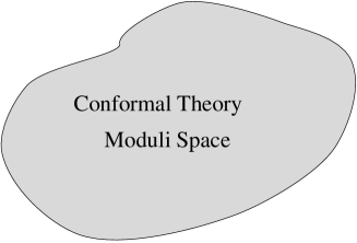
Figure 10: Schematic drawing of the Moduli Space of an $N=2$ theory.

Each point in this moduli space corresponds to one $N=2$ superconformal theory. We can deform any given theory into another by using the truly marginal operators. It can be shown that, at least locally, the conformal field theory Zamolodchikov metric on this moduli space is block diagonal between the $\Phi_{(1,1)}$-type and $\Phi_{(-1,1)}$-type marginal operators and hence we can think of moduli space as being a metric product (at least locally) of the schematic form shown in figure 11.

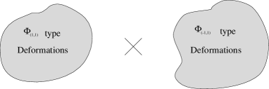
Figure 11: The two sectors of an $N=2$ moduli space.

One of our main goals is to fully understand this picture in detail, especially when we are starting from an initial theory realized as an $N=2$ superconformal sigma model on some Calabi-Yau space. So, to begin imagine we build an $N=2$ superconformal field theory as a non-linear sigma model on a Calabi-Yau target space $M$. Can we give a geometrical interpretation to the two types of marginal operators (that we expect to exist if $c>3$ so $h_{\rm{max}}=c/6>1/2$)?

The answer to this question comes immediately from the association between $(c,c)$ and $(a,c)$ fields and harmonic differential forms. That is, we already described the way in which $(c,c)$ fields with $(h=1/2,\overline{h}=1/2)$ correspond to harmonic $(2,1)$-forms and how $(a,c)$ fields with $(h=1/2,\overline{h}=1/2)$ correspond to harmonic $(1,1)$-forms. This essentially establishes the geomtrically meaning of the abstract conformal field theory operators, when the latter is constructed as a nonlinear sigma model. To see this in a bit more detail, let us look at the corresponding $\Phi_{(-1,1)}$ marginal operator. To lowest order, the $(a,c)$ field can be written as $b_{i\bar{\jmath}}\lambda^{i}\psi^{\bar{\jmath}}$ with $b_{i\bar{\jmath}}$ being a harmonic $(1,1)$-form on $M$. Using the map between $(a,c)$ fields and marginal operators given above, we map this to $G^{+}_{-1/2}\bar{G}^{-}_{-1/2}$ $(b_{i\bar{\jmath}}\lambda^{i}\psi^{\bar{\jmath}})$. To lowest order again, this is $b_{i\bar{\jmath}}\partial X^{i}\bar{\partial}X^{\bar{\jmath}}$. This operator, as in the case of the circle, deforms the “size” of $M$, i.e., the Kähler form $ig_{i\bar{\jmath}}dX^{i}\wedge dX^{\bar{\jmath}}$ on $M$. Hence, these conformal field theory marginal operators correspond to geometrical deformations of the Kähler structure on the Calabi-Yau manifold. Similarly, the $\Phi_{(1,1)}$, which give pure-index type metric perturbations, deform the “shape” of $M$ — i.e., the complex structure of $M$. The notion of deforming the complex structure and Kähler structure of a Calabi-Yau manifold, while still preserving the Calabi-Yau conditions, thus has a direct conformal field theory manifestation in terms of deformation by truly marginal operators.

For those readers less comfortable with the mathematics of such deformations, the following figure illustrates their effect in the case of a one-dimensional Calabi-Yau manifold, namely the torus. The original torus is drawn with a solid line and its deformed versions are drawn with dotted lines. A Kähler deformation leaves the shape (the angle between the cycles) fixed, but changes the volume. A complex structure deformation leaves the volume fixed, but changes the shape.

Figure 12: Kähler and Complex structure deformations of a torus.

We have thus found that corresponding to the two types of operators that can deform our $N=2$ superconformal theory to a nearby theory, there are two geometrical operations that deform a Calabi-Yau manifold to a nearby manifold, without spoiling the Calabi-Yau conditions. This gives the geometrical interpretation of figure 10 in the form given by figure 13.

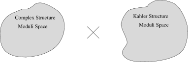
Figure 13: Geometrical interpretation of the conformal field theory moduli space.

This is the geometrical interpretation of $N=2$ superconformal field theory moduli space that was subscribed to for some time.

We will return to this picture repeatedly and see that the geometrical counterpart to the conformal field theory moduli space is deficient in a number of ways. In other words, figure 13 is quite incomplete as it presently stands. Eradicating these deficiencies will lead us to a number of remarkable mathematical and physical features.

As a presage to that discussion, let us note one fact: The distinction between the $\Phi_{(1,1)}$ and $\Phi_{(-1,1)}$ type marginal operators, at the level of conformal field theory is rather trivial, being just the sign of a $U(1)$ charge. The distinction between their geometrical counterparts — harmonic (1,1)-forms and harmonic (2,1)-forms — is comparatively dramatic. These two types of forms are mathematically quite different. This is a strange asymmetry to which we shall return.

5 Interrelations Between Various N = 2 Superconformal Theories

At the end of section 3 we described three general ways of constructing $N=2$ superconformal field theories: non-linear sigma models, Landau-Ginzburg theories and minimal models. Our goal now is to try to understand the relationship between these theories. We will proceed by finding pairwise connections.

5.1 Landau-Ginzburg Theories and Minimal Models

Consider a Landau-Ginzburg theory with a single chiral superfield $\Psi$:

$$S=\int d^{2}zd^{4}\theta\,K(\Psi,\bar{\Psi})+\left(\int d^{2}zd^{2}\theta\,W(\Psi)+c.c.\right)~{}.$$

Take $W(\Psi)=\Psi^{P+2}$. In [82] the authors calculate the central charge $c_{P}$ of this Landau-Ginzburg theory at its infrared fixed point to be

$$c_{P}=6\left({1\over 2}-{1\over P+2}\right)={3P\over P+2}~{}.$$

Recall that the unitary $c<3,~{}N=2$ superconformal theories are the minimal models. Thus, we learn that a Landau-Ginzburg theory of this particular form is, at its conformally invariant infrared fixed point (assuming such a point exists) the $P$-th minimal model, $MM_{P}$. (In fact, to be a bit more precise, it is the $P$-th minimal model with the so called A-modular invariant.) For more information supporting this statement of equivalence and emphasis on subtleties which arise, the reader should consult [112]. Thus, the Landau-Ginzburg theories with the simplest possible superpotential gives the Lagrangian realization of the minimal models.

5.2 Minimal Models And Calabi-Yau Manifolds: A Conjectured Correspondence

Conformally invariant non-linear sigma models with Calabi-Yau target spaces have central charge $c=3d$, where $d$ is the complex dimension of the Calabi-Yau space. As we have discussed, the $MM_{P}$ have central charges $c={{3P\over P+2}}<3$. Thus, for $d>1$ it would not seem that there could be any connection between these types of conformal theories. However, given a collection of $r$ conformal theories with central charges $c_{i},~{}i=1,...,r$, one can build a new conformal field theory — the tensor product theory — with central charge $c=\sum_{i=1}^{r}c_{i}$. The Hilbert space of this theory is the tensor product of the Hilbert spaces of the constituent models and the energy-momentum tensor takes the form

$$T=\sum_{i=1}^{r}\,1\otimes\cdots\otimes 1\otimes T_{i}\otimes 1\otimes\cdots\otimes 1~{}.$$ (5.1)

In fact, since the operation of orbifolding by a finite discrete group does not change the central charge of a conformal theory, a quotient of the above tensor product will also have central charge $c=\sum_{i=1}^{r}c_{i}$. Applying this to the minimal models, we see that if we choose a collection of integers $P_{i},i=1,...,r$ such that

$$\sum_{i=1}^{r}{{3P_{i}\over P_{i}+2}}=3\,d~{},$$

then the tensor product of these conformal theories and orbifolds thereof will have central charge $3d$. In principle, then, there might be some relationship between the $MM_{P}$ combined in this manner with Calabi-Yau sigma models.

The first evidence that there is such a relationship was found by Gepner [53, 54]. As we discussed, it has long been known that a string theory of the form we are studying, $M_{4}\times\{{\rm an}\ N=2,~{}c=9\ {\rm superconformal\ field\ theory\ }\}$, has space-time supersymmetry if and only if the superconformal theory has odd integral $U(1)_{L}$ and $U(1)_{R}$ charge eigenvalues. Following this lead, Gepner considered a tensor product of minimal models with $\sum_{i=1}^{r}{{3P_{i}\over P_{i}+2}}=9$ orbifolded onto a spectrum with odd integral $U(1)$ charges. That is, he considered $[MM_{P_{1}}\times\cdots\times MM_{P_{r}}]|_{\rm U(1)\ projected}$, which we denote by $(P_{1},...,P_{r})$. Gepner then compared the symmetries and massless space-time spectra of a particular case $(P_{1},P_{2},P_{3},P_{4},P_{5})$ $=$ $(3,3,3,3,3)$ with that of the best studied Calabi-Yau sigma model with $c=9$ given by the vanishing locus of $z_{1}^{5}+z_{2}^{5}+...+z_{5}^{5}$ in ${\mathbb{C}}P^{4}$. He found these data to be essentially identical (up to some additional massless particles in the minimal model formulation which were expected to generically become massive under small perturbations). It was further shown in [41] that the Yukawa couplings (whose form we will discuss) as computed in the minimal model formulation and in the Calabi-Yau formulation for this and a couple of other examples also agreed. These results gave additional support to Gepner’s conjecture that the minimal model construction yields conformal theories interpretable as non-linear sigma models on particular Calabi-Yau manifolds. Again, this is quite surprising as the minimal model formulation does not appear to have any geometrical content.

This conjecture was initially put on firmer foundation in the works of [63, 85, 86] and more thoroughly [113]. Each of these gives a procedure for identifying which Calabi-Yau manifold should correspond to a given minimal model construction; the paper of [63] gives a heuristic path integral argument establishing a direct link between the two types of constructions and [113] provides a rigorous argument uncovering a rich phase structure (also found in [4]).

We now briefly review these arguments establishing a link between (orbifolds of) tensor product minimal model constructions and Calabi-Yau sigma models.

5.3 Arguments Establishing Minimal-Model/Calabi-Yau Correspondence

Each of the papers [63, 85, 86, 113] makes use of the accepted isomorphism between the minimal model theory at level $P$ and the Landau-Ginzburg theory of a single chiral superfield $X$ with superpotential $W=X^{P+2}$, described above. In particular, since Hamiltonians (and hence Lagrangians) of tensor product theories add, we immediately learn from our previous discussion that $\otimes_{j=1}^{r}MM_{j}$ is isomorphic to the conformally invariant Landau-Ginzburg model with action

$$S=\int d^{2}zd^{4}\theta\,\sum_{j=1}^{r}K_{j}(X_{j},\overline{X}_{j})+\left(\int d^{2}zd^{2}\theta\,\sum_{j=1}^{r}X_{j}^{P_{j}+2}+h.c.\right)~{}.$$ (5.2)

We reemphasize that the explicit form of the kinetic terms consistent with conformal invariance can not generally be written down, but should be thought of as being determined by the fixed points of a renormalization group flow.

We now specialize to the case of $r=d+2$. A simple but crucial point [63] to note is that the minimal model condition of

$$\sum_{j=1}^{d+2}{{3P_{j}\over P_{j}+2}}=3d$$

implies that $D$, the least common multiple of the $P_{j}+2$, satisfies

$$D=\sum_{j=1}^{d+2}{{D\over P_{j}+2}}~{}.$$

This implies that if we interpret the superpotential $W$ in (5.2) to be an equation

$$\sum_{j=1}^{d+2}\,X_{j}^{P_{j}+2}=0$$

in the weighted projective space $W{\mathbb{C}}P^{d+1}(D\omega_{1}\cdots D\omega_{d+2})$ (although nothing justifies this interpretation as yet), with

$$\omega_{i}\equiv{{1\over P_{i}+2}}~{},$$

then it is well defined (homogeneous of degree $D$) and its locus satisfies the condition that $D$ equals the sum of the weights of the projective space. Using our earlier discussion of classical geometry, we can see that this ensures that the resulting space is Calabi-Yau. To see this, we note that the weighted projective space generalization of (2.69) is

$$c(W{\mathbb{C}}P^{4}(w_{1},w_{2},w_{3},w_{4},w_{5}))=\prod_{i=1}^{5}\,(1+w_{i}J)~{}.$$ (5.3)

Then, the generalization of (2.73) is

$$c(TW)={{\prod(1+w_{i}J)\over(1+DJ)}}=1+(\sum w_{i}-D)J+\cdots~{}.$$ (5.4)

Vanishing of the first Chern class thus requires the degree $D$ to be the sum of the weights $w_{i}$ of the weighted projective space. At the moment, though, nothing in our discussion justifies ascribing such an interpretation to $W$. Following [63] we can, however, give at least a heuristic justification.

We consider (5.2) and note that since the Kähler potential is irrelevant we may choose it at will, and in particular we may choose it very small. To a first approximation, in fact, we may ignore it. The path integral representing the partition function of the theory now becomes

$$\int\left[{\cal D}X_{1}\right]\ldots\left[{\cal D}X_{r}\right]\,e^{i\int\,d^{2}\!zd^{2}\!\theta\,(W(X_{1},\ldots,X_{r})+{\rm c.c.})}~{}.$$ (5.5)

In a patch of field space in which $X_{1}\neq 0$, we can rewrite the path integral (5.5) in terms of new variables

$$\xi_{1}^{\omega_{1}}=X_{1}~{};~{}~{}~{}~{}~{}\xi_{i}={X_{i}\over\xi_{1}^{\omega_{i}}}~{}.$$ (5.6)

Since

$$W(X_{1},\ldots,X_{r})\equiv W^{\prime}(\xi_{1},\ldots,\xi_{r})=\xi_{1}\,W^{\prime}(1,\xi_{2},\ldots,\xi_{r})~{},$$ (5.7)

(5.5) becomes

$$\int\left[{\cal D}\xi_{1}\right]\ldots\left[{\cal D}\xi_{r}\right]\,J\,e^{i\int d^{2}\!zd^{2}\!\theta\,\xi_{1}(W^{\prime}(1,\xi_{2},\ldots,\xi_{r})+{\rm c.c.})}~{},$$ (5.8)

where $J$ is the Jacobian for the change of variables, and is given by

$$J=\xi_{1}^{\nu}~{},~{}~{}~{}~{}~{}\nu=1-\sum_{i=1}^{r}\omega_{i}~{}.$$ (5.9)

If $\nu=0$, then $J$ is a constant, and the integration over $\xi_{1}$ in (5.8) yields a delta function $\delta(W^{\prime}(1,\xi_{2},\ldots,\xi_{r}))$, constraining the remaining fields to lie on the manifold $W=0$. Proceeding in like fashion with the other fields, we can cover field space with patches, in each of which we obtain a similar result. We note, though, that the change of variables we have used to simplify the path integral is not one-to-one. In fact, upon inspection we see that $\xi_{i}$ are invariant under the transformation

$$X_{i}\rightarrow e^{2\pi i\omega_{i}}\,X_{i}~{}.$$ (5.10)

The $X_{i}$ are thus naturally interpreted as homogeneous coordinates on $W{\mathbb{C}}P^{4}($ $D\omega_{1}$, $\cdots$, $D\omega_{d+2})$. However, because of this invariance, the model we have shown to be equivalent to propagation on the manifold $W=0$ in this projective space is not the theory (5.2) but rather the quotient of this by the transformation (5.10). Since the charge of $X_{i}$ is $\omega_{i}$, this is precisely the quotient by $g_{0}=e^{2\pi iJ_{0}}$ required to obtain a consistent (space-time supersymmetric) string vacuum [53, 54, 108], as we discussed in section 3. Many properties of the resulting model may be extracted from the superpotential alone, as discussed in [82]. An important role in this equivalence was played by the fact that the Jacobian for the transformation to homogeneous coordinates was constant. For $r=5$ this is simply the condition that the central charge $c=9$. And, as we have seen, this is precisely the condition that the hypersurface $W=0$ have vanishing first Chern class [63].

There are a few relevant remarks we should make.

1. The connection between Landau-Ginzburg theory and Calabi-Yau sigma models has been most easily achieved by first deforming away from the conformally invariant theories (by manipulating the Kähler form), finding an isomorphism and then allowing the renormalization group to appropriately adjust kinetic terms to reestablish conformal invariance. Nothing in our argument assures that the resulting kinetic term in the Calabi-Yau sigma model will be sufficiently “large” to ensure that sigma model perturbation theory will be valid. Hence, such a Calabi-Yau sigma model would only truly be defined via analytic continuation. This is precisely what happens in the more rigorous approach to relating Landau-Ginzburg theories to Calabi-Yau sigma models discussed in the next section.

2. We have made a number of specializations in our discussions. First, we have focused attention on the case of $r$, the number of minimal models, being equal to $d+2$. Second, we have restricted attention to the A-invariants. Although we shall not discuss it in detail here, both of those specializations can be substantially relaxed.

3. Although compelling, the argument of [63] has some obvious deficiencies. Paramount amongst these is the manipulation of the kinetic energy terms in the Landau-Ginzburg action. As shown in the appendix of [63] one can work with a more conventional kinetic term, although the argument does become a bit cumbersome and delicate.

Finally, we note that subsequent to the above arguments, Witten reexamined this correspondence and found a more robust and satisfying argument which also points out a number of important subtleties. We now briefly review this approach. Our discussion will be limited to the simplest possible case of a Calabi-Yau hypersurface with $h^{1,1}=1$, i.e. the quintic hypersurface. More general complete intersections are treated in [113] and from the viewpoint of toric geometry in [5].

Witten begins with neither the Calabi-Yau sigma model nor the Landau-Ginsburg model. Rather, he starts with an $N=2$ supersymmetric gauge theory (called the “linear sigma model”) with gauge group $U(1)$ and action

$$S=S_{\rm kinetic}+S_{W}+S_{\rm gauge}+S_{\rm FI-D\ term}~{},$$ (5.11)

where the only terms whose precise form we need to explicitly write are $S_{W}$ and $S_{\rm FI-D\ term}$. In particular,

$$S_{W}=\int d^{2}zd^{2}\theta\,W(P,S_{1},...,S_{5})~{},$$ (5.12)

where $W$ is the superpotential of the theory, $P,S_{1},...,S_{5}$ are chiral superfields whose $U(1)$ charges are $-5,1,...,1$ respectively, and $W$ takes the $U(1)$ invariant form

$$W=P\,G(S_{1},...,S_{5})~{}.$$ (5.13)

$G$ is a homogeneous transverse quintic in the $S_{i}$. $S_{\rm FI-D\ term}$ is the supersymmetric Fayet-Iliopoulos $D$-term. The important point for our present discussion is that the bosonic potential of the theory takes the form

$$U=|G(s_{i})|^{2}+|p|^{2}\sum_{i}\left|{\partial G\over\partial s_{i}}\right|^{2}+{1\over 2e^{2}}\,D^{2}+2|\sigma|^{2}\,\left(\sum_{i}\,|s_{i}|^{2}+25|p|^{2}\right)~{},$$ (5.14)

with

$$D=-e^{2}\,\left(\sum_{i}\,|s_{i}|^{2}-5|p|^{2}-r\right)~{}.$$ (5.15)

In this expression lower case letters represent scalar components of the corresponding capital letter superfields and $\sigma$ is a scalar field coming from the twisted chiral multiplet whose presence is quite important but shall not play a central role in our discussion.

Our goal is to study the classical ground states of this theory for various choices of the parameter $r$. It turns out that there are two qualitatively different answers depending upon the sign of $r$. Let us study the two possibilities in turn.

First, let us take $r>0$. Minimizing the $D$-term in $U$ then implies that not all $s_{i}$ can vanish. Assuming $G$ to be a transverse quintic polynomial then implies that not all $|{{\partial G\over\partial s_{i}}}|$ vanish and hence minimizing $U$ forces $p=0$. Furthermore, with at least one $s_{i}$ non-zero we learn that $\sigma=0$ and finally, minimizing $U$ further implies $G=0$ and

$$\sum_{i}\,|s_{i}|^{2}=r~{}.$$ (5.16)

We are not quite done in our identification of the ground state because not all such configurations are distinct due to the gauge symmetry of the model. Rather, we have the $U(1)$ identifications

$$(s_{1},...,s_{5})\sim(e^{i\theta}s_{1},...,e^{i\theta}s_{5})~{}.$$ (5.17)

How can we picture the meaning of the conditions we have found? At first sight, the fields $s_{1},...,s_{5}$ live in ${\mathbb{C}}^{5}$. The combined constraints (5.16) and (5.17), however, take us from ${\mathbb{C}}^{5}$ to ${\mathbb{C}}P^{4}$. This is nothing but the statements from classical geometry embodied in (2.58) and (2.59). By way of review, note that the equivalence relation of projective space $(z_{1},...,z_{5})\sim\lambda(z_{1},...,z_{5})$ can be used to pick out one representative of each class. We can do this by enforcing conditions on the coordinates which uniquely pick out a value of $\lambda$ for a given choice of initial coordinates $(z_{1},...,z_{5})$. Notice that (5.16) and (5.17) do precisely this and hence allow us to interpret the $s_{i}$ as living in ${\mathbb{C}}P^{4}$. Thus, the other condition of $G=0$ yields the vanishing of a quintic polynomial in ${\mathbb{C}}P^{4}$ — the familiar quintic Calabi-Yau hypersurface. Thus, for $r>0$ the fields are constrained to lie on this Calabi-Yau manifold and hence our original $U(1)$ gauge theory reduces to this Calabi-Yau sigma model. We note, as discussed in [113] that the original Lagrangian has other fields not present in the Calabi-Yau sigma model whose masses are determined by the value of $r$. Thus, for $r>>0$, these fields play no role and hence in this limit we actually are recovering the Calabi-Yau manifold not only as the ground state, but also as governing the effective quantum field theory. In the infrared limit any non-zero mass field drops out and hence in the conformal limit we as well regain the conformally invariant non-linear sigma model.

Let us also note that $r$ determines the “size” of the Calabi-Yau manifold from (5.16). In this sense, the variable $r$ can be thought of as determining the Kähler modulus of the theory. We hasten to add, though, that as we let the theory flow to the infrared and simultaneously integrate out the massive degrees of freedom, the value of $r$ will change à la the Wilson renormalization group. Hence, the actual value of the Kähler modulus at the infrared fixed point will in general be determined by $r$ but will not be equal to it. The parameter $r$ is often called the “algebraic” coordinate on the moduli space. It is the natural variable for the linear sigma model. The value of the Kähler modulus $\widetilde{r}$ at the infrared fixed point is often called the “sigma-model” coordinate as it is the natural variable from the latter point of view. For more discussion on these points see [113, 6].

Having discussed the case of $r>0$, let us move on to the case of $r<0$. Reasoning exactly as we did above, we find that all of the $s_{i}$ must vanish, $p$ is constrained to be ${\sqrt{{-r\over 5}}}$, and there is an unbroken ${\mathbb{Z}}_{5}$ symmetry group (because $p$ has charge 5). Hence, unlike the case $r>0$, the vacuum state is not an extended space, but rather is unique: geometrically it is a point. Furthermore, from the form of the potential, the $s_{i}$ are massless fluctuations about this vacuum state. The configuration space, therefore is ${\mathbb{C}}^{5}/{\mathbb{Z}}_{5}$. Now, from our earlier discussion, this is an orbifold of a Landau-Ginzburg theory since the latter can be described as a theory with a unique vacuum state with some number of massless fields. The ${\mathbb{Z}}_{5}$ identifications coming from the unbroken gauge group gives rise to the stated orbifolding. We note that this ${\mathbb{Z}}_{5}$ action is in fact nothing but the action of $e^{2\pi iJ_{0}}$ and hence constitutes the required $U(1)$ projection that we have discussed earlier. It plays exactly the same role as the required identifications, from the non-linear change of variable, in the path integral argument given previously.

Thus, by varying the parameter $r$ in (5.11), it has been shown [113] that we interpolate between a linear sigma model on a Calabi-Yau space and a Landau-Ginzburg orbifold. By allowing the renormalization group to act, we thereby interpolate between the conformally invariant limits of these two types of theories. We might re-emphasize here the important point that the reason we should take $|r|$ to be large in each regime is to suppress the massive excitations which would cause the theory obtained to differ from a non-linear sigma model or a Landau-Ginzburg model. After we flow to an infrared fixed point by the renormalization group, though, any initial non-zero mass, no matter how small, becomes effectively infinite. Thus, so long as we ultimately flow to an infrared fixed point, the size of $|r|$ can be arbitrarily small.

As we mentioned, from (5.15), we see that the actual value of $r$, for $r$ positive, sets the overall size of the ambient projective space — i.e. $r$ determines its Kähler form; by restriction to the Calabi-Yau hypersurface $r$ determines its Kähler form as well. For $r$ negative, its actual value sets the expectation of twist fields in the Landau-Ginzburg theory [113]. Hence, in the language of section 3, $r$ may be thought of as a Kähler moduli space parameter and the moduli space (for this simple discussion) consisting of ${\mathbb{R}}$ divided into two regions $r>0$ and $r<0$. Physically, the former region has a point (the “deep interior point”) with $r$ being infinite corresponding to an infinite volume Calabi-Yau space. The latter region of $r<0$ contains its own deep interior point of $r$ being negative infinity which we have identified as the Landau-Ginzburg orbifold point. (It is at this point, for example, that the theory has an enhanced quantum symmetry [108, 113].) We call the first region of the moduli space the Calabi-Yau sigma model region and the second region the Landau-Ginzburg orbifold region.

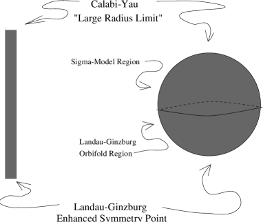
Figure 14: The Kähler moduli space for the example discussed.

The left hand side of figure 14 shows the $r$ moduli space. It is just the real line. Now, as is well known, string theory instructs us to complexify the variable $r$ by combining it with an antisymmetric tensor field $r\rightarrow t=b+ir$. A special feature of $b$ is that shifts of its value by an integer, in the domain of large $r$, do not affect the theory, and hence the natural complex variable to use is $w=e^{2\pi i(b+ir)}$. In this way we can map the sigma model region of the moduli space to the upper hemisphere of a sphere. One can give similar arguments for the Landau-Ginzburg region [4, 113, 7] and in this way obtain a natural compactification of the complexified moduli space, as shown in the right hand side of figure 14. We see that this moduli space consists of two regions or “phases” and it can be shown that there is no obstruction to smoothly varying the complex parameter $t$ to move from one phase to the other.

Points in the first region correspond to Calabi-Yau sigma models with Kähler class determined by the precise location of the point; points in the second region correspond to Landau-Ginzburg orbifolds with value of the twist field being determined by the location of the point. As we try to move from the first region to the second (or vice versa) conformal perturbation theory about the deep interior point in region one (or region two, going in the other direction) breaks down. In the sigma model region this is merely the statement that if the Calabi-Yau gets too small, the expansion parameter $(\alpha^{\prime})^{2}/r$ gets big and perturbation theory will be invalid. However, using the results of [4] and [113] we know that the conformal theories corresponding to almost all points in the moduli space are perfectly well defined, even if a perturbative understanding of them breaks down, and hence we can smoothly continue our journey along such a path in the moduli space. As a matter of convention, if a theory can be described via conformal perturbation theory around one of our deep interior points, then we categorize it as belonging to the same type of theory as this deep interior point. This justifies the names we have given to the two regions above: points within the region in the $r>0$ sector of figure 13 are called Calabi-Yau sigma models while those in a similar region in the other sector are called Landau-Ginzburg orbifold theories. An important point is that if we allow for analytic continuation, then we can make sense of a perturbative expansion about the deep interior point of the $r>0$ sector for essentially any point in the moduli space, even with $r<0$. Thus, in this sense, we can even think of the deep interior point in the Landau-Ginzburg orbifold sector as being (the analytic continuation of a) Calabi-Yau sigma model with a particular (identifiable) Kähler class. In terms of the parameter $r$, we see that this special choice seems to require a negative Kähler class, or more precisely, an analytic continuation to a negative Kähler class. We should note, though, that in [6] it was shown that the physics of the situation implies that physical radii $\widetilde{r}$ (and their analytic continuations) which arise from integrating out massive modes in the linear sigma model, are non-trivial functions of the $r$ parameter which appear to always be non-negative. Thus, in this sense, one can interpret the result of [113] to say that a Landau-Ginzburg orbifold conformal model (of the type considered here) is equivalent to the analytic continuation of a conformally invariant non-linear sigma model on a Calabi-Yau space to a particular (and identifiable [108, 113, 6]) “small and positive” value of the Kähler class.

Pictorially, the situation we are describing is illustrated by figures 15 and 16 where we show the one-parameter moduli space of the quintic hypersurface in algebraic and then in non-linear sigma model variables. Details can be found in [6, 30].

Figure 15: A slice of the linear sigma model moduli space.

Figure 16: A slice of the non-linear sigma model moduli space.

We see, therefore, that this relatively rigorous argument lays out quite clearly the relationship between Calabi-Yau  conformal field theories and conformally invariant Landau-Ginzburg orbifold theories. We first pass to non-conformal members in the same universality class as these theories, which we see to be different “phases” of the same overarching theory (5.11) related by different values for the parameter $r$ (more precisely, $t$). As we pass to the conformally invariant limit, the parameter $r$ turns into the Kähler modulus, $\widetilde{r}$. When $\widetilde{r}$ is sufficiently large, nonlinear sigma model perturbation theory converges, and we have a direct geometrical interpretation of a string moving through an ambient spacetime. If $\widetilde{r}$ is not in this range of convergence, the resulting model, at first sight, loses a geometrical interpretation. However, the results of [6] indicate that even these regions have a geometric interpretation, so long as we appropriately analytically continue from the large radius geometric region. In this way, for instance, we see above that the Landau-Ginsburg point in the quintic moduli space can be interpreted as a nonlinear sigma model with real Kähler class ${4\over 5}\,\sin^{3}({2\pi\over 5})>0$ (see [30] for details of the derivation of this value). This is beyond the range of non-linear sigma model perturbation theory, but can be fully analysed via analytic continuation.

In our discussion of [113] we have limited our attention to theories with one Kähler modulus, and hence one $r$ parameter. For Calabi-Yau manifolds with an $h^{1,1}$ dimensional Kähler moduli space, there will be $h^{1,1}$ $r$ parameters, $r_{1},...,r_{h^{1,1}}$. The moduli space will again naturally divide itself into phase regions, however the structure will typically be far richer than the two phase regions found in the one-dimensional setting. We can again describe theories in each region in terms of the most natural interpretation of their corresponding deep interior point. There will typically be a Landau-Ginzburg orbifold region, numerous smooth Calabi-Yau regions (with the various Calabi-Yau spaces being birationally equivalent but possibly topologically distinct), Calabi-Yau orbifold regions and regions consisting of hybrids of these. Again, the work of [6] indicates that all of these regions — in the conformally invariant limit — have the property that they can be thought of as a nonlinear sigma model on a Calabi-Yau target space with a sensible Kähler modulus. By sensible we mean that it is non-negative with respect to at least one Calabi-Yau topology. We will discuss some of this in later sections; for further details the reader should see [113, 4, 6].

6 Mirror Manifolds

In our discussion to this point, we have seen that there are certain abstract properties of $(2,2)$ superconformal theories that can be realized by a variety of field theoretic constructions. For instance, there is a nice correspondence between geometrical constructs in the non-linear sigma model formulation and their abstract conformal field theoretic counterparts. Furthermore, in general there are two types of marginal operators in an abstract $c=9,\ (2,2)$ superconformal theory and that these correspond to the two geometrical ways of deforming a Calabi-Yau manifold without spoiling the Calabi-Yau conditions.

We note, however, that there is an uncomfortable asymmetry between the abstract conformal field theory description and the geometrical realization. Namely, the two kinds of conformal field theory marginal operators differ only in a rather trivial way: the conventional sign of a $U(1)$ charge. On the other hand, their geometrical counterparts differ far more significantly: the cohomology groups $H^{1}(M,T)$ and $H^{1}(M,T^{\star})$ (that is, $(d-1,1)$-forms, after contracting with $\Omega$ and $(1,1)$-forms) are vastly different mathematical objects. It is surprising that such a pronounced geometrical distinction finds such a trivial conformal field theory manifestation. This led the authors of [42] and [82] to speculate on a possible resolution: if for each Calabi-Yau manifold $M$ there was a second Calabi-Yau $\widetilde{M}$ corresponding to the same conformal field theory but with the association of $H^{1}(\widetilde{M},T)$ and $H^{1}(\widetilde{M},T^{\star})$ to conformal field theory marginal operators reversed relative to that of $M$, the asymmetry would be resolved. Each conformal field theory marginal operator would then be interpretable geometrically either as a Kähler or as a complex structure deformation, provided one chooses the Calabi-Yau manifold realization judiciously.

Although an interesting idea, at the time of these speculations there was no evidence for the existence of such pairs of Calabi-Yau manifolds corresponding to the same conformal field theory. Subsequently, two simultaneous independent developments changed this. In [27] the authors generated, via computer, numerous Calabi-Yau manifolds embedded in weighted projective four-dimensional space. The data so generated consisted almost completely of pairs of manifolds $(M,\widetilde{M})$ satisfying

$$\begin{array}[]{c}\dim H^{1}(M,T)=\dim H^{1}(\widetilde{M},T^{\star})~{},\\ \dim H^{1}(M,T^{\star})=\dim H^{1}(\widetilde{M},T)~{}.\end{array}$$ (6.1)

This, of course, is a necessary condition for $M$ and $\widetilde{M}$ to be identified with the same conformal field theory as above, however it is far from sufficient. Two quantum field theories can have sectors with the same number of fields, but yet be otherwise completely unrelated. In [64], on the other hand, an explicit construction of pairs of Calabi-Yau manifolds $M$ and $\widetilde{M}$ satisfying (6.1) and corresponding to the same conformal field theory was given. Using the fact that $H^{1}(M,T)\cong H^{1,1}(M)$ and $H^{1}(M,T^{\star})\cong H^{d-1,1}(M)$, one can phrase (6.1) as

$$\begin{array}[]{c}h^{1,1}(M)=h^{d-1,1}(\widetilde{M})~{},\\ h^{d-1,1}(M)=h^{1,1}(\widetilde{M})~{},\end{array}$$ (6.2)

where $h^{i,j}(M)=\dim H^{i,j}(M)$. In particular, this implies that the Hodge diamond for $\widetilde{M}$ is a mirror reflection through a diagonal axis of the Hodge diamond for $M$. For this reason, we chose [64] the term mirror manifolds for such pairs $(M,\widetilde{M})$. The construction of [64], therefore, established conclusively that mirror manifolds exist. As of this writing, this is the only established construction of mirror manifolds and hence shall be the focus of the present section. There have been a number of other conjectured constructions of mirror manifolds from both physicists and mathematicians (including the work of [27] alluded to above) and these are discussed in the review paper of Berglund and Katz [20]. Recently, Strominger, Yau and Zaslow [107] have proposed that mirror symmetry can be thought of as T-duality on toroidal fibers of particular Calabi-Yau spaces.

6.1 Strategy of the construction

Before discussing the details of the mirror manifold construction of [64], we now briefly describe the general strategy of our approach. Let ${\cal C}$ be a conformal field theory associated with a Calabi-Yau manifold $M$. ${\cal C}$ may be thought of as the non-linear sigma model with $M$ as a target space or, somewhat more generally, ${\cal C}$ may be thought of as the equivalence class of conformal theories (regardless of the details of their particular construction) which are isomorphic to this non-linear sigma model. There are many operations one can perform upon ${\cal C}$ to generate a new conformal theory ${\cal C^{\prime}}$ (or a new equivalence class ${\cal C^{\prime}}$ of conformal theories). For instance, earlier we discussed the operations of deformation by truly marginal operators which yield a new conformal theory from some chosen initial conformal model. In general, not all operations which take one conformal theory to another have a geometrical interpretation. In such a case, the resulting theory ${\cal C^{\prime}}$ may no longer be associated with a Calabi-Yau manifold. In other words, in the equivalence class ${\cal C^{\prime}}$, there need not be a conformal theory constructed from a non-linear sigma model. As our interest here is in the geometrical interpretation of conformal field theories, we will henceforth restrict our attention to operations $\Gamma$ taking ${\cal C}$ $\rightarrow$ ${\cal C^{\prime}}$ which have a functorial geometric realization. In plain language, we focus on $\Gamma$ such that if the non-linear sigma model on $M$ is in the class ${\cal C}$, then the non-linear sigma model on $\Gamma(M)=\widetilde{M}$ is in the class $\Gamma($${\cal C}$$)=$ ${\cal C^{\prime}}$.

Amongst the operations $\Gamma$ which have this property is the operation of taking the quotient of ${\cal C}$ by a discrete symmetry group $G$, so long as $G$ has a geometrical interpretation as a holomorphic isometry preserving the holomorphic $(d,0)$ form on the associated Calabi-Yau space. In common parlance this is referred to as orbifolding [43, 44] by $G$. Equivalently, this operation amounts to gauging the discrete group $G$ as we shall discuss later. From the geometrical viewpoint, orbifolding by the group $G$ has the effect of yielding a new space $\Gamma(M)=M/G$ which is characterized by the identification of all points $x,y$ in $M$ which are related by

$$x=g(y)~{}{\rm with}~{}g\in G~{}.$$ (6.3)

If there are points $x$ in $M$ such that $x=g(x)$, then $x$ is called a fixed point and $M/G$ (usually) acquires a singularity at $x$.

Now, let us imagine that we can find an operation $\Gamma$ which has a geometric realization and such that:

1. $\Gamma({\cal C})\ {\rm is\ isomorphic\ to}\ {\cal C}.$ This would imply that the non-linear sigma models on $M$ and $\Gamma(M)$ are isomorphic as conformal field theories. Such distinct spaces $M$ and $\Gamma(M)$ which nonetheless give rise to the same conformal field theory are known as classically string equivalent [65].

2. The explicit map realizing the isomorphism between ${\cal C}$ and $\Gamma({\cal C})$ is changing the sign of the right moving $U(1)_{R}$ charge of each operator in ${\cal C}$.

3. The map between operators in the conformal field theory and geometrical constructs in the associated Calabi-Yau space (as discussed in section 3) is independent of $\Gamma$.

We claim that if such an operation $\Gamma$ meeting conditions (1)-(3) can be found, then $M$ and $\Gamma(M)=\widetilde{M}$ would constitute a mirror pair of Calabi-Yau spaces.

To see why, let us consider ${\cal C}$ and $M$ as described with the property, say, that marginal operators with $U(1)_{L}\times U(1)_{R}$ charges $(-1,1)$ are associated with the cohomology group $H^{1,1}(M)$ and marginal operators with charges $(1,1)$ are associated with the cohomology group $H^{d-1,1}(M)$. Now, let us apply $\Gamma$. By property $(1)$, $\Gamma$ has a geometrical interpretation and hence we can construct a new Calabi-Yau space $\Gamma(M)=\widetilde{M}$ corresponding to the conformal theory $\Gamma({\cal C})$. By property $(3)$, the cohomology groups $H^{1,1}(\widetilde{M})$ and $H^{d-1,1}(\widetilde{M})$ correspond to the marginal operators in $\Gamma({\cal C})$ with $U(1)_{L}\times U(1)_{R}$ charges $(-1,1)$ and $(1,1)$ respectively. By property $(2)$, we see therefore that the cohomology groups $H^{1,1}(\widetilde{M})$ and $H^{d-1,1}(\widetilde{M})$ are associated with marginal operators in ${\cal C}$ with $U(1)_{L}\times U(1)_{R}$ charges $(1,1)$ and $(-1,1)$ respectively. Hence, $M$ and $\widetilde{M}$ are string equivalent (they correspond to isomorphic conformal field theories) and they satisfy (6.2). This means that they constitute a mirror pair. In the following sections we shall show that a suitable operation $\Gamma$ can in fact be constructed. Before doing so, however, we should emphasize one subtle point. As we have discussed, the $N=2$ superconformal field theories we study are often part of continuous families of theories. We let ${\cal F}(\cal C)$ denote the family of theories which are all related to ${\cal C}$ via deformation by truly marginal operators. Now, note that if we can find an operation $\Gamma$ meeting conditions $(1)-(3)$ for any theory ${\cal C}^{\prime}\subset$ ${\cal F}(\cal C)$, then such an operation exists for all other theories in ${\cal F}(\cal C)$. The reason for this is as follows. Let ${\cal C}^{\prime}$ and ${\cal C}$ both belong to ${\cal F}(\cal C)$ and be related via

$${\cal C}^{\prime}={\cal U}({\cal{C}})~{},$$ (6.4)

where ${\cal U}$ denotes the appropriate marginal operator deformation. Now, if $\Gamma$ is the operation meeting conditions (1)$-$(3) for ${\cal C}^{\prime}$, then the operation

$${\widetilde{\cal U}}^{-1}\circ\Gamma\circ{\cal U}$$ (6.5)

meets conditions $(1)-(3)$ when acting on ${\cal C}$. By definition, ${\widetilde{\cal U}}^{-1}$ is the inverse deformation of ${\cal U}$ composed with explicitly changing the sign of all $U(1)_{R}$ eigenvalues. Thus, so long as we can find an operation $\Gamma$ meeting $(1)-(3)$ for one theory in ${\cal F}(\cal C)$, we are assured of such an operation for every theory in the family. We note, further, that oftentimes only some subset of all of the theories in ${\cal F}(\cal C)$ will have a natural geometric interpretation in terms of a Calabi-Yau sigma model. The meaning of conditions (1) and $(3)$ for these theories is that when a candidate operation $\Gamma$ is transported via (6.5) to theories in ${\cal F}(\cal C)$ with a non-linear sigma model interpretation (assuming such points exist in the family), then conditions (1) and $(3)$ are met there.

6.2 Minimal Models and their Automorphisms

As discussed in the last section, an important ingredient in the construction of mirror manifolds is an understanding of the minimal model conformal field theories. We now turn to a more detailed discussion of these models.

The superconformal primary fields of the $P$-th minimal model are labeled by six integers, $l,m,s,\bar{l},\bar{m},\bar{s}$ and are typically written $\Phi_{s,\bar{s}}^{l,m,\bar{l},\bar{m}}(z,\bar{z})$. The meaning of these indices is made clear by recalling that the $N=2$ $P$-th minimal model is isomorphic to the coset of an $SU(2)$ WZW model at level $P$ by a $U(1)$ subgroup together with a free boson. That is,

$$MM_{P}={{SU(2)_{P}\over U(1)}}\times{\rm free~{}boson}~{}.$$ (6.6)

In other words, we remove a free boson at one radius by dividing out the $U(1)$ and we put a free boson back at a different radius. Now, primary fields of an $SU(2)$ WZW model are labeled, in part, by their usual $SU(2)$ angular momentum quantum numbers $l,m$ with $|m|\leq l$; this is the meaning of the indices $l,m$ (and $\bar{l},\bar{m}$ ) in $\Phi_{s,\bar{s}}^{l,m,\bar{l},\bar{m}}(z,\bar{z})$, and these indices satisfy the same inequality. In fact, to avoid dealing with half-integral values of spin, $l$ and $m$ are defined to be twice their $SU(2)$ counterparts and hence $m$ can range from $-l$ to $l$ in steps of two. With this convention, the value of $l$ can range up to $P$. The index $s$ arises as a convenient bookkeeping device. Namely, it proves convenient to split the Verma module built upon a given superconformal primary field into those states which differ from the primary field by the action of an even versus an odd number of supercurrents $G^{\pm}$. In the NS sector, we take the value of $s$ to be zero or two; the former referring to states which differ from the highest weight state by the action of an even number of supercurrents (therefore including the bona fide original primary field) and the latter referring to states obtained by the action of an odd number of supercurrents. In the R sector, we define $s$ to be one or three with these values playing an analogous role (we can equivalently replace three by $-1$ since this index is only defined modulo four). The index $s$ is referred to as the ‘fermion’ number.

More concretely, if we temporarily ignore the $s$ index and all of the anti-holomorphic dependence, superconformal primary fields in the NS sector can be labeled $\Phi_{l,m}$ with conformal weights

$$h={{l(l+2)\over 4(P+2)}}-{{m^{2}\over 4(P+2)}}$$

and $U(1)$ charge

$$Q={{m\over P+2}}$$

(and similarly for the suppressed anti-holomorphic sector). The chiral primary fields, i.e. those for which $G^{+}_{-1/2}$ also annihilates the corresponding state, have $m=l$ and the antichiral primary fields ($G^{-}_{-1/2}$ annihilates the corresponding state) have $m=-l$. In the Ramond sector, our primary fields can be written as $\Psi^{\pm}_{l,m}$ where $\pm$ refers to whether the state is annihilated by $G_{0}^{+}$ or by $G_{0}^{-}$. Then, the conformal weights of such states are

$$h={{l(l+2)\over 4(P+2)}}-{{(m\pm 1)^{2}\over 4(P+2)}}+{{1\over 8}}$$

and their $U(1)$ charges are

$$Q={{m\pm 1\over P+2}}\pm{{1\over 2}}~{}.$$

Ramond states annihilated by both operators $G_{0}^{\pm}$ form the Ramond ground states and have

$$h={P\over 8(P+2)}~{}.$$

The Ramond ground states are $\Psi^{+}_{l,l}$ and $\Psi^{-}_{l,-l}$. Now let us reintroduce the $s$ index. We define $\Phi^{l,m}_{s}$ to be:

$$\Phi_{l,m}~{},\quad {\rm for} ~{}s=0~{},$$

$$\Psi_{l,m}^{+}~{},\quad {\rm for} ~{}s=1~{},$$

$$\Psi_{l,m}^{-}~{},\quad {\rm for} ~{}s=-1~{},$$

$$G^{\pm}\Phi_{l,m}~{},\quad {\rm for} ~{}s=2~{},$$

and the index $s$ is defined modulo four, so this is a complete list. Now, the last definition might seem ambiguous, but in fact we will only use this notation to describe the Verma module (modulo fermion number as discussed) ${\cal H}^{l,m}_{s}$ to which these states belong and both $G^{\pm}\Phi_{l,m}$ lie in the same Verma module (and have the same fermion number mod 2).

Now, given such a field $\Phi_{s}^{l,m}(z,\bar{z})$, we consider the character $\chi^{l,m}_{s}$ defined by

$$\hbox{$\chi^{l}_{m,s}$}(\tau,z,u)\equiv\hbox{$\>e^{-2\pi iu}\>$}\,\hbox{{\bigrm Tr}\kern-10.50005pt\lower 9.04166pt\hbox{$\scriptstyle{\cal H}^{l}_{m,s}$}}\,\!\!\!\!\!\!\!~{}\left[\hbox{$\>e^{2\pi izJ_{0}}\>$}\hbox{$\>e^{2\pi i\tau(L_{0}-c/24)}\>$}\right]~{}.$$ (6.7)

We re-emphasize that the trace is taken over a projection ${\cal H}^{l}_{m,s}$ to definite fermion number (mod 2) of a highest weight representation of the (right-moving) $N=2$ algebra with highest weight vector $\Phi^{l;\overline{l}}_{q,s;\overline{q},\overline{s}}(0)$, with fermion number 1 assigned to the superpartners $G^{\pm}$ of the energy-momentum tensor, as discussed in the last paragraph.

Our goal is to put together such chiral characters in a modular invariant way to construct a consistent partition function. To do so, we must first understand how the characters transform under modular transformations. This was worked out in [53, 54] and the results are:

$$\hbox{$\chi^{l}_{q,s}$}(\tau+1) = e^{\pi i{l(l+2)\over 2(P+2)}}\,e^{\pi i\left(-{q^{2}\over 2(P+2)}+{s^{2}\over 4}\right)}\,\hbox{$\chi^{l}_{q,s}$}(\tau)~{},$$ (6.8)

$$\hbox{$\chi^{l}_{q,s}$}(-1/\tau) = {1\over\sqrt{2}(P+2)}\,\sum_{l^{\prime}+q^{\prime}+s^{\prime}=0\,{\rm mod}\,2}\sin\left[\pi{(l+1)(l^{\prime}+1)\over P+2}\right]\,e^{\pi i\left({qq^{\prime}\over P+2}-{ss^{\prime}\over 2}\right)}\,\hbox{$\chi^{l^{\prime}}_{q^{\prime},s^{\prime}}$}(\tau)~{}.~{}~{}$$ (6.9)

An important observation is that the modular transformation properties factor into three pieces, each of which only acts on precisely one of the three indices labeling the characters. In fact, this is the real motivation for introducing the auxiliary $s$ index in the first place. We recognize that the index $l$ transforms under the representation of the modular group carried by level $P$ affine $SU(2)$ characters, while the indices $m$ and $s$ transform under the representations carried by level $-(P+2)$ and level $2$ theta functions respectively. We can, therefore, construct modular invariant combinations of these characters by combining known modular invariants for these three types of objects. Up to discrete quotients, the general modular invariant combination takes the form:

$$Z={1\over 2}\!\!\!\!\!\!\!\sum_{{\scriptstyle l,\overline{l},m,s}\atop{\scriptstyle l+m+s=0\,{\rm mod}\,2}}\!\!\!\!\!\!\!\!\!\!\!A_{l,\overline{l}}~{}\hbox{$\chi^{l}_{m,s}$}\,\hbox{$\chi^{\overline{l}\,*}_{m,s}$}~{},$$ (6.10)

where $A_{l,\overline{l}}$ is any one of the $ADE$ classified affine modular invariants at level $P+2$. (The factor of $1\over 2$ reflects the identifications on the fields discussed in, for example, [53, 54].)

We would now like to note the following important facts for the minimal model conformal theories.

1. $MM_{P}$ is invariant under a ${\mathbb{Z}}_{2}\times{\mathbb{Z}}_{P+2}\times{\overline{{\mathbb{Z}}}}_{2}\times{\overline{{\mathbb{Z}}}}_{P+2}$ discrete symmetry group.

2. The orbifold ${{MM_{P}\over{\mathbb{Z}}_{P+2}}}$ of $MM_{P}$ with respect to the diagonal group ${\mathbb{Z}}_{2}\times{\mathbb{Z}}_{P+2}$ is a new conformal theory ${\widetilde{MM_{P}}}$ which is isomorphic to $MM_{P}$. The map from ${\widetilde{MM_{P}}}$ to $MM_{P}$ is: change the sign of the $U(1)_{R}$ eigenvalue associated with each field.

These facts were first noted in [56] and, in reality, go back to [118]. In the latter paper, the authors realized the $MM_{P}$ as a combination of level $P$ parafermions and a free boson. The level $P$ parafermions have a ${\mathbb{Z}}_{P}$ discrete symmetry the action of which via orbifolding is to produce an isomorphic theory. When combined with the free boson, this ${\mathbb{Z}}_{P}$ is promoted to ${\mathbb{Z}}_{P+2}$; the action of orbifolding by the latter is again to produce an isomorphic theory. For $P=2$, the parafermion system is an ordinary fermion and the isomorphism of this theory with a ${\mathbb{Z}}_{2}$ orbifold of itself is nothing other than familiar order-disorder duality in the Ising model. Hence one can think of property (2) above as a generalization of this well known duality.

Explicitly, the discrete symmetry action can be written as

$$g_{q}\cdot\Phi^{l;\overline{l}}_{q,s;\overline{q},\overline{s}} = e^{2\pi i{q\over P+2}}\,\Phi^{l;\overline{l}}_{q,s;\overline{q},\overline{s}}~{},$$ (6.11)

$$g_{s}\cdot\Phi^{l;\overline{l}}_{q,s;\overline{q},\overline{s}} = e^{2\pi i{s\over 2}}\,\Phi^{l;\overline{l}}_{q,s;\overline{q},\overline{s}}\>~{}.$$ (6.12)

The second of these is a ${\mathbb{Z}}_{2}$ symmetry which such theories also respect. In essence it is charge conjugation.

As property (2) is of central importance, let us look at it more closely. We can establish property $(2)$ in two ways. The first is via direct calculation and the second is via manipulation of a path integral representation of these theories. We will go through the first approach.

6.3 Direct Calculation

Let us define $Z$ by (6.10). More generally, we define $Z[x,y]$ to be a twisted counterpart to the theory described by (6.10), where the boundary conditions of all fields are twisted by the operator $e^{2\pi i(J_{0}+\overline{J}_{0})x}$ in the time direction and by $e^{2\pi i(J_{0}+\overline{J}_{0})y}$ in the space direction. For fields with these boundary conditions, the partition function $Z[x,y]$ can be shown to be given by

$$Z[x,y]=\!\!\!\!\!\!\!\sum_{{\scriptstyle l,\overline{l},m,s}\atop{\scriptstyle l+m+s=0\,{\rm mod}\,2}}\!\!\!\!\!\!\!\!\!\!e^{-2\pi ix{m+\overline{m}\over 2(P+2)}}\,A_{l,\overline{l}}\,\hbox{$\chi^{l}_{m,s}$}\,\hbox{$\chi^{\overline{l}\,*}_{m-2y,s}$}~{}.$$ (6.13)

How does one get this result? The simplest way is to directly write down $Z[x,0]$ — this is easy since it simply involves inserting a factor depending on the charge of each highest weight state into (6.10). Then, by successive modular transformations, using (6.8) and (6.9), we can derive (6.13). In what follows, we shall drop explicit reference to the sums over $\scriptstyle l,s$ as they are not involved in any non-trivial way.

We now create a new theory from (6.10) by taking the quotient, in the sense of conformal theory, of (6.10) by the left-right symmetric ${\mathbb{Z}}_{P+2}$ symmetry group. By standard results in conformal field theory,

$$Z_{\rm new}={1\over P+2}\,\sum_{x,y=0,...,P+1}\,Z[x,y]~{}.$$ (6.14)

Using our results from above,

$$Z_{\rm new}={1\over P+2}\,\sum_{x,y,m}e^{-2\pi ix{(m+\widetilde{m})\over 2(P+2)}}\,\hbox{$\chi^{l}_{m,s}$}\,\hbox{$\chi^{\overline{l}\,*}_{\widetilde{m},s}$}~{},$$ (6.15)

where $\widetilde{m}=m-2y$. Now, performing the sum on $m$ we learn $2m-2y=0\,{\rm mod}~{}(2(P+2))$ to get a non-zero contribution. Hence, $\widetilde{m}=-m\,{\rm mod}~{}(2(P+2))$. By the symmetries above we can thus write

$$Z_{\rm new} = {1\over P+2}\,\sum_{y,m}\,\hbox{$\chi^{l}_{m,s}$}\,\hbox{$\chi^{\overline{l}\,*}_{-m,s}$}$$ (6.16)

$$= \sum_{m}\hbox{$\chi^{l}_{m,s}$}\,\hbox{$\chi^{\overline{l}\,*}_{-m,s}$}~{}.$$

Now, to actually divide by $e^{2\pi i(J_{0}+\overline{J}_{0})y}$, as noted, we need to include the $s$ dependence of the charge as well. This amounts to dividing by the ${\mathbb{Z}}_{2}$ action given earlier; the calculation is essentially identical to that given and yields the final result

$$Z_{\rm new}=\sum_{m}\hbox{$\chi^{l}_{m,s}$}\,\hbox{$\chi^{\overline{l}\,*}_{-m,-s}$}~{}.$$ (6.17)

Now, let us examine this new theory. Notice that it differs from the original theory (6.10) only in that the $U(1)$ charges in the anti-holomorphic sector all have opposite sign to those in (6.10). But the overall sign of this charge is simply a matter of convention. That is, when we built the invariant (6.10), we could equally well have written

$$Z={1\over 2}\!\!\!\!\!\sum_{{\scriptstyle l,\overline{l},m,s}\atop{\scriptstyle l+m+s=0\,{\rm mod}\,2}}\!\!\!\!\!\!\!\!\!A_{l,\overline{l}}\,\,\hbox{$\chi^{l}_{m,s}$}\,\hbox{$\chi^{\overline{l}\,*}_{-m,-s}$}$$ (6.18)

and gotten an isomorphic theory (with the explicit isomorphism mapping a field in the theory based on (6.10) to the field in (6.18) with opposite sign of right-moving $U(1)$ charge.

Thus we conclude that $Z_{\rm new}$ is not a new theory, after all. It is, in fact, isomorphic to the original minimal model theory $MM_{P}$ represented by the partition function $Z$ that we began with. Notice that this is true regardless of which of the $ADE$ invariants we use in constructing $Z$.

Having established that orbifolding $MM_{P}$ by its ${\mathbb{Z}}_{P+2}$ discrete symmetry group yields an isomorphic theory with the isomorphism simply being a change in the sign of all $U(1)_{R}$ eigenvalues, we see that we are part way along the path of realizing the strategy for constructing mirror manifolds described previously. We now extend this result to products of minimal models and hence to the Calabi-Yau spaces that we can associate to them.

6.4 Constructing Mirror Manifolds

In this subsection we will combine some of the results of the preceding two sections to realize the strategy, outlined previously, for the construction of mirror manifolds.

We have seen that the $N=2$ minimal models admit an operation, orbifolding, which produces an isomorphic conformal theory related to the original by a change in the sign of all $U(1)_{R}$ eigenvalues. We have also seen that there is an intimate connection between minimal models and Calabi-Yau sigma models. The point of this section is to show that through the minimal-model/Calabi-Yau connection, we can transport the orbifolding operation on individual minimal models to an operation $\Gamma$ meeting the three conditions discussed in section 6.1 and thereby yield a construction of mirror manifolds. We should emphasize at the outset of our discussion that we will be making use of the comment made at the end of section 6.1 regarding the fact that we need only demonstrate the existence of a suitable operation $\Gamma$ at one point in the moduli space of theories $\cal F(\cal C)$ related to $\cal C$ by truly marginal deformation to ensure that such an operation exists at all points. Furthermore, we can even work at a point in the moduli space whose natural interpretation is not in terms of a Calabi-Yau sigma model (such as a Landau-Ginzburg orbifold region). The meaning of conditions (1)-(3) of section 6.1 in this setting, as discussed, is that when transported à la (6.5) to a Calabi-Yau sigma model region in the moduli space, the resulting operation satisfies conditions (1)-(3).

We will focus our detailed remarks on moduli spaces which contain a smooth Calabi-Yau region corresponding to a complex $d$-dimensional Calabi-Yau hypersurface of Fermat type in weighted projective space. Such moduli spaces, as we have seen, also contain a region corresponding to one of the $c=3d$ minimal model constructions discussed in section 5.3 represented most conveniently as a Landau-Ginzburg orbifold theory. As we shall mention at the end, the analysis directly extends to any Calabi-Yau theory whose moduli space contains a minimal model region.

Following our remarks above, our explicit analysis will take place at the deep interior point of the Landau-Ginzburg orbifold region in the Kähler moduli space and at the Fermat point in the complex structure moduli space. In other words, our calculations will take place at the conformal field theory corresponding to the minimal model construction. We will see that we can construct a suitable operation $\Gamma$ at this point, and by transporting it to the smooth Calabi-Yau region in the moduli space construct a mirror to the original manifold. (We should note that we could also interpret the minimal model point as the analytic continuation of a Calabi-Yau sigma model, as discussed above and then our explicit analysis constructs the analytic continuation of a sigma model on the mirror Calabi-Yau space.)

Consider, then, the tensor product of $s$ minimal model theories orbifolded onto integral $U(1)$ charges, $(P_{1},...,P_{s})$, with

$$\sum_{j=1}^{s}{{3P_{j}\over P_{j}+2}}=3d~{}.$$

We recall our notation:

$$(P_{1},...,P_{s})=[MM_{P_{1}}\otimes...\otimes MM_{P_{s}}]|_{U(1)\ \rm projected}~{}.$$ (6.19)

By the result of section 6.3, we can write

$$(P_{1},...,P_{s})\equiv\left[{MM_{P_{1}}\over{\mathbb{Z}}_{P_{1}+2}}\otimes...\otimes{MM_{P_{s}}\over{\mathbb{Z}}_{P_{s}+2}}\right]\Bigg{|}_{U(1)\ \rm projected}~{},$$ (6.20)

with the explicit isomorphism being the changing of the sign of all $U(1)_{R}$ eigenvalues. Now, we claim:

$$\left[{MM_{P_{1}}\over{\mathbb{Z}}_{P_{1}+2}}\otimes...\otimes{MM_{P_{s}}\over{\mathbb{Z}}_{P_{s}+2}}\right]\Bigg{|}_{U(1)~{}\rm projected}={{[MM_{P_{1}}\otimes...\otimes MM_{P_{s}}]|_{U(1)\ \rm projected}}\over G}$$ (6.21)

where $G$ is the maximal subgroup of ${\mathbb{Z}}_{P_{1}+2}\times...\times{\mathbb{Z}}_{P_{s}+2}$ by which one can orbifold and preserve the integrality of the $U(1)$ charges of the theory. In particular, the action of $G$ is

$$(\Phi_{1},...,\Phi_{s})\rightarrow(e^{2\pi i{n_{1}\over q_{1}}}\,\Phi_{1},...,e^{2\pi i{n_{s}\over q_{s}}}\,\Phi_{s})~{},$$ (6.22)

for arbitrary integers $(n_{1},...,n_{s})$ such that $\sum_{j=1}^{s}n_{j}/q_{j}$ is an integer.

Establishing this claim requires a calculation that can be found in [64, 66]. For our discussion here we simply note that it is a familiar fact in conformal field theory that successive quotients of a theory can undo each other if the subsequent quotients are quantum versions of the previous one. All we have here is an example of this phenomenon. The $U(1)$ projection has the effect of undoing those quotients of the theory that do not respect (6.22).

Thus, we have shown that

$$(P_{1},...,P_{s})\equiv{(P_{1},...,P_{s})\over G}~{},$$ (6.23)

with the isomorphism between the two theories being a reversal in the sign of all $U(1)_{R}$ eigenvalues of the fields in the left hand side relative to the right hand side.

Since this operation of orbifolding is independent of the Kähler modulus of the theory, it is trivial to transport it to a smooth Calabi-Yau region. The action on the Calabi-Yau manifold $M$,

$$z_{1}^{P_{1}+2}+\dots+z_{P_{s}}^{P_{s}+2}=0~{},$$ (6.24)

in the weighted projective space $W{\mathbb{C}}P^{s-1}({D\over P_{1}+2},...,{D\over P_{s}+2})$ with arbitrary Kähler form is given by

$$(z_{1},...,z_{s})\rightarrow(e^{2\pi i{n_{1}\over q_{1}}}\,z_{1},...,e^{2\pi i{n_{s}\over q_{s}}}\,z_{s})~{},$$ (6.25)

for arbitrary integers $(n_{1},...,n_{s})$ such that $\sum_{j=1}^{s}n_{j}/q_{j}$ is an integer. This condition, which defines $G$, is interpretable in the Calabi-Yau region as the condition of preserving the holomorphic $d$-form $\Omega$ on $M$.

Now, this operation of orbifolding by $G$ meets conditions $(1)$ and $(2)$ of section 6.1: since it is true at the minimal model point it is true everywhere in the moduli space, as discussed. This operation also meets condition (3) as can most quickly be seen in the following way: consider a conformal field $\Lambda$ associated with a geometrical harmonic form $a_{\Lambda}$, such that $\Lambda$ and hence $a_{\Lambda}$ are invariant under the action of $G$ (there always will be at least one such field: the restriction of the Kähler class of the ambient projective space to $M$). Then, in the theory based on $M/G$, $\Lambda$ and $a_{\Lambda}$ again correspond. This implies that if marginal operators of charges $(1,1)$ and $(1,-1)$ are associated to elements of $H^{1}(M,T^{\star})$ and $H^{1}(M,T)$ respectively (or vice versa), then the same association holds in the theory based on $M/G$. Namely, marginal operators of charges $(-1,1)$ and $(1,1)$ are associated to elements of $H^{1}(M/G,T^{\star})$ and $H^{1}(M/G,T)$ respectively (or vice versa). This is so because the association of conformal fields to geometrical cohomology can only take two possible forms (as explicitly noted). One established association of a conformal field and a geometrical harmonic form distinguishes between these two possibilities. Since we have shown that in both $M$ and $M/G$ we have at least one identical association, we are done. Hence, our operation meets condition $(3)$ as well.

Thus, we have shown that the Calabi-Yau hypersurface $M$ given by (6.24) (for arbitrary choice of Kähler form) has mirror given by $M/G$. Let us note that following our discussion of the phase structure of the moduli space of these theories, it is more appropriate to say the following. Let $M$ be a Calabi-Yau manifold. It belongs to a moduli space of conformal theories. Consider $M/G$. It is a Calabi-Yau space (it is not smooth) which also belongs to a family of conformal theories. We have shown that for each point in the first moduli space there is a corresponding point in the second moduli space giving rise to an isomorphic theory. Thus, mirror symmetry is more precisely a statement of pairs of families of conformal theories.

6.5 Examples

In this section we give a few examples which illustrate the construction of the last section. The following two tables show mirror pairs of theories constructed via the orbifolding operation above. The column ‘symmetries’ denotes the group action by which we quotient. For instance, in the first table, $[0,0,0,1,4]$ indicates that we take the quotient by the ${\mathbb{Z}}_{5}$ action

$$(z_{1},z_{2},z_{3},z_{4},z_{5})\rightarrow(z_{1},z_{2},z_{3},\alpha z_{4},\alpha^{4}z_{5})~{},$$ (6.26)

where $\alpha$ is a fifth root of unity. Mirror pairs reside in symmetric positions in the tables with respect to the horizontal axis through the center.

Table 1: Orbifolds of the theory $(P_{1},P_{2},P_{3},P_{4},P_{5})=(3,3,3,3,3)$.

    Theory Symmetries $$h^{2,1} h^{1,1} \chi -200 -88 -40 (3,3,3,3,3) -8 z_{1}^{5}+\cdots+z_{5}^{5}=0 {\mathbb{C}}P^{4}$$     101 1       [0,0,0,1,4] 49 5       [0,1,2,3,4] 21 1       [0,1,1,4,4] [0,1,2,3,4] 21 17       or [0,1,1,4,4] 17 21 8       [0,1,3,1,0] [0,1,1,0,3] 1 21 40       in [0,1,4,0,0] [0,3,0,1,1] 5 49 88     [0,1,2,3,4] [0,1,1,4,4] 1 101 200 [0,0,0,1,4]    

Table 2: Orbifolds of theory $(P_{1},P_{2},P_{3},P_{4})=(3,8,8,8)$.

    Theory Symmetries $$h^{2,1} h^{1,1} \chi -288 -192 -72 -48 (3,8,8,8) -48 -24 z_{1}^{5}+z_{2}^{10}+\cdots+z_{4}^{10}+z_{5}^{2}=0 W{\mathbb{C}}P^{4}(2,1,1,1,5)$$     145 1       [0,0,5,5] 99 3       [0,2,2,6] 47 11       [0,0,1,9] 39 15       [0,0,2,8] 37 13       or [0,1,2,7] 29 17       [0,5,4,1] 17 29 24       in [0,8,1,1] 15 39 48       [0,5,5,0] [0,8,1,1] 13 37 48       [0,5,5,0] [0,1,9,0] 11 47 72       [0,0,1,9] [0,8,0,2] 3 99 192       [0,0,1,9] [0,1,1,8] 1 145 288    

6.6 Implications

Having reviewed the initial speculations and subsequent work which established the existence of mirror symmetry, we would now like to turn to a discussion of the implications of this phenomenon, as well as some important work applying mirror symmetry to interesting and explicit examples.

The general lesson learned from mirror manifolds is that there is a duality in Calabi-Yau moduli space since we have two distinct geometrical descriptions of a single physical situation. Moreover, perturbation theory in each model is governed by the respective Kähler parameters as the coupling expansion is in terms of $\alpha^{\prime}/R^{2}$ (where, more precisely, $R^{2}$ denotes the area of rational curves as measured by the relevant Kähler form.) We have seen, though, that Kähler parameters of one Calabi-Yau determine complex structure parameters of the other, and vice versa. Thus, if the Kähler parameters of one Calabi-Yau are “small” thereby making perturbation theory suspect, its complex structure can be adjusted so that the Kähler structure of its mirror will be nice and “big”, thereby ensuring the efficacy of perturbation theory. In other words, mirror symmetry gives rise to a strong/weak sigma-model coupling duality. We will exploit this in an important physical context in the next chapter. For now, we would like to briefly indicate one other specific implication of mirror symmetry.

Let $M$ and $\widetilde{M}$ be mirror Calabi-Yau manifolds each corresponding to the conformal field theory ${\cal C}$. Consider a (non-vanishing) three-point function of conformal field theory operators corresponding to $(2,1)$-forms on $M$. We will not explicitly do the calculation here, but as shown in [104] (and rederived in [41] in a slightly different way) this correlation function is given by the simple integral on $M$ (2.80)

$$\int_{M}\Omega^{abc}\,\widetilde{b}^{(i)}_{a}\wedge\widetilde{b}^{(j)}_{b}\wedge\widetilde{b}^{(k)}_{c}\wedge\Omega~{},$$ (6.27)

where, as explained earlier, the $\widetilde{b}^{(i)}_{a}$ are $(2,1)$-forms (expressed as elements of $H^{1}(M,T)$ with their subscripts being tangent space indices). Due to the non-renormalization theorem proved in [41], we know that this expression (6.27) is the exact conformal field theory result. By mirror symmetry, these same conformal field theory operators correspond to particular and identifiable $(1,1)$-forms on the mirror $\widetilde{M}$, which we can label $b^{(i)}$. Mathematically, due to the absence of a non-renormalization theorem, the expression for such a coupling in terms of geometric quantities on $\widetilde{M}$ is comparatively complicated:

$$\int_{{\widetilde{M}}}b^{(1)}\wedge b^{(2)}\wedge b^{(3)}+\sum_{m,\{u\}}\hbox{$\>e^{-\int_{{\mathbb{C}}P^{1}}u_{m}^{*}(J)}\>$}\left(\int_{{\mathbb{C}}P^{1}}u^{*}(b^{(1)})\int_{{\mathbb{C}}P^{1}}u^{*}(b^{(2)})\int_{{\mathbb{C}}P^{1}}u^{*}(b^{(3)})\right)~{},$$ (6.28)

where (as derived in [105, 38, 39, 30, 31, 9]) the $b_{(i)}$ are elements of $H^{1}(\widetilde{M},T^{\star})$, $\{u\}$ is the set of holomorphic maps to rational curves on $\widetilde{M}$, $u:{\mathbb{C}}P^{1}\rightarrow\Gamma$ (with $\Gamma$ such a holomorphic curve), $\pi_{m}$ is an $m$-fold cover ${\mathbb{C}}P^{1}\rightarrow{\mathbb{C}}P^{1}$ and $u_{m}=u\circ\pi_{m}$. $J$ refers to the Kähler form on $\widetilde{M}$. The infinite series of corrections in this expression arise from string world sheet configurations that wrap around rational curves (essentially two-spheres) embedded in $\widetilde{M}$. Just like instantons in the more familiar setting of gauge theories, these string configurations are topologically nontrivial and contribute nonperturbative corrections to correlation functions. These corrections are an explicit examples of how ‘stringy’ geometry differs from ordinary classical geometry. The first term in this correlation function is a familiar mathematical construct — the intersection form of $\widetilde{M}$. The infinite series of instanton corrections move us away from classical geometry; they are stringy in origin as they arise because the extended nature of the string allows it to encircle homologically nontrivial cycles as it moves.

Now, since both (6.27) and (6.28) correspond to the same conformal field theory correlation function, they must be equal; hence we have [64]

$$\int_{{M}}\Omega^{abc}\widetilde{b}^{(i)}_{a}\wedge\widetilde{b}^{(j)}_{b}\wedge\widetilde{b}^{(k)}_{c}\wedge\Omega\!\!\!\! = \!\!\!\!\int_{{\widetilde{M}}}b^{(i)}\wedge b^{(j)}\wedge b^{(k)}$$

$$+ \!\!\!\!\sum_{m,\{u\}}\,\hbox{$\>e^{\int_{{\mathbb{C}}P^{1}}u_{m}^{*}(J)}\>$}\left(\int_{{\mathbb{C}}P^{1}}u^{*}(b^{(i)})\right)\left(\int_{{\mathbb{C}}P^{1}}u^{*}(b^{(j)})\right)\left(\int_{{\mathbb{C}}P^{1}}u^{*}(b^{(k)})\right)~{}.$$

Notice the crucial role played by the underlying conformal field theory in deriving this equation. If we simply had two manifolds whose Hodge numbers were interchanged we could not, of course, make any such statement. This result [64] is rather surprising and clearly very powerful. We have related expressions on a priori unrelated manifolds which probe rather intimately the structure of each. Furthermore, the left hand side of (6.6) is directly calculable while the right hand side requires, among other things, knowledge of the rational curves of every degree on the space.

The equality (6.6) is another striking example of quantum geometry. First, as mentioned, the coupling (6.28) has as its leading term a familiar expression from classical geometry. However, there are corrections arising from the extended nature of the string as this allows for homotopically non-trivial field configurations sensitive to the rational curves on the manifold. Second, the fact that the resulting expression is equal to (6.27) on a different space is a hallmark feature of quantum geometry: the distinctions of classical geometry ‘smear’ and can be erased in the quantum setting. We emphasize that every correlation function in the underlying conformal theory now has two geometrical interpretations. The equality (6.6) is but one such example. In principle, we could write down scores of others.

Since written, (6.6) has been verified in several illuminating examples [87, 48, 78, 83, 18, 29, 74] pioneered by the papers [30, 31]. These authors showed that one could use (6.6) to determine the number of rational curves of arbitrary degree on $\widetilde{M}$, a question of mathematical interest that was previously unsolved. This brought to the forefront the tremendous calculation power of mirror symmetry. In the next section we shall see an impressive physical consequence of string theory that mirror symmetry allows us to establish.

7 Space-Time Topology Change — The Mild Case

This section is based in part on [11].

7.1 Basic Ideas

The essential lesson of general relativity is that the geometrical structure of space-time is governed by dynamical variables. That is, the metric changes in time according to the Einstein equations. In the usual formulations of general relativity, the space-time metric is defined on a space of fixed topological type — the “size” and “shape” of the space can smoothly change, but the underlying topology does not. A natural question to ask is whether this formulation is too restrictive; might the topology of space itself be a dynamical variable and hence possibly change in time? This issue has long been speculated upon. Heuristically, one suspects that topology might be able to change by means of the violent curvature fluctuations which would be expected in any quantum theory of gravity. Just as the fluctuations of the magnetic field in a box of size $L$ are on the order of $(\hbar c)^{1/2}/L^{2}$, those of the curvature of the gravitational field are on the order of $({\hbar G\over c^{3}})^{1/2}/L^{3}$. Thus, on extremely small scales, say $L\sim L_{\rm Planck}$, huge curvature fluctuations are unsuppressed. One can imagine that such curvature fluctuations could “tear” the fabric of space resulting in a change of topology. The expected discontinuities in physical observables accompanying the discontinuous operation of a change in topology would be hidden, one hopes, behind the smoothing effects of quantum uncertainty. Of course, without a true theory of quantum gravity, one cannot make quantitative sense of such hypothesized processes.

With the advent of string theory, we are led to ask whether any new quantitative light is shed on the issue of topology change. A number of works have addressed aspects of this question, and in this and the next section, we shall review the results in three of them [113, 4, 67]. In the first two of these papers, the first definitive evidence that there are physically smooth processes in string theory which result in a change in the topology of space-time was given. These processes occur at string tree level and hence are essentially classical phenomena. Their unusual character therefore arises from the extended nature of the string. The type of topology change in these works is relatively mild in that the Hodge numbers of the Calabi-Yau stay fixed while only more subtle invariants (such as the cubic intersection form) change. In [67], on the other hand, quantum effects are taken into account — in fact, non-perturbative effects having to do with solitonic degrees of freedom. In this more robust setting, it is shown that there are physical processes that result in rather drastic topology changing transitions — transitions which change even the Hodge numbers of the Calabi-Yau compactification. Here we discuss the case of mild topology change and later return to the more drastic case.

7.2 Mild Topology Change

In this subsection we focus on the results of [113, 4]. We will see the first evidence of physically smooth topology changing processes in string theory. Furthermore, as phenomena in string theory, these processes are not at all exotic. Rather, they correspond to the most basic kind of operation arising in conformal field theory: deformation by a truly marginal operator. From a space-time point of view, this corresponds to a slow variation in the vacuum expectation value of a scalar field which has an exactly flat potential. It is crucial to emphasize, as remarked above, that these physically smooth topology changing processes occur even at the level of classical string theory. It is not, as had been suspected from point particle intuition, that quantum effects give rise to topology change, but, rather, it is the extended structure of the string which bears responsibility for this effect.

We can immediately summarize here the essential content of [113] and [4]. From the viewpoint of classical general relativity or the classical non-linear sigma model, we know that there are constraints on the metric tensor which appears in the action. Namely, since the metric is used to measure lengths, areas, volumes, etc., it must satisfy a set of positivity conditions. For instance, if we have a non-linear sigma model on a Kähler target space $M$ with metric $g_{\mu\overline{\nu}}$, we can write the Kähler form of the metric as $J=ig_{\mu\overline{\nu}}dX^{\mu}\wedge dX^{\overline{\nu}}$. The latter must satisfy

$$\int_{M_{r}}J^{r}>0~{},$$ (7.1)

where $M_{r}$ is an $r$-dimensional (complex) submanifold of $M$ and $J^{r}$ represents the $r$-fold wedge product of $J$ with itself. The set of real closed $2$-forms which satisfy (7.1) is a subset of $H^{2}(X,{\mathbb{R}})$ known as the Kähler cone and is schematically depicted in figure 17. This figure should be thought of as a more precise version of the drawing of the Kähler moduli space in figure 13, in which we did not pay attention to details such as positivity. Such Kähler forms manifestly span a cone because if $J$ satisfies (7.1), then so does $sJ$ for any positive real $s$.

Figure 17: A Kähler cone.

The burden of [113] and [4] is that, in string theory, (7.1) can be relaxed and still result in perfectly well behaved physics. As discussed, the Kähler form of a target Calabi-Yau space is one of the moduli fields of the associated conformal field theory. Investigation of the conformal field theory moduli space reveals that the corresponding geometrical description necessarily involves configurations in which the (supposed) Kähler form lies outside of the Kähler cone of the particular Calabi-Yau being studied. In fact, any and all choices of an element of $H^{2}(X,{\mathbb{R}})$ give rise to well defined conformal field theories. In [113, 4] it was shown that some of these configurations can be interpreted as non-linear sigma models on Calabi-Yau manifolds of topological type distinct from the original. With respect to this Calabi-Yau of new topology, the Kähler modulus satisfies (7.1) and hence may be thought of as residing in a new Kähler cone which shares a common wall with the original (figure 18). Furthermore, there is no physical obstruction to continuously deforming the underlying conformal field theory so that its geometrical description passes from one Kähler cone to another and hence results in a change in topology of the target space — i.e. of space itself.

Figure 18: Adjoining Kähler cones.

Philosophically, this result is providing us with another important way in which classical geometry fails to capture qualitative properties of string physics. A change in topology is, by its basic mathematical definition, a process which is not smooth. However, quantum geometry, the proper geometry for describing string physics, allows for topology change in a perfectly smooth manner.

To understand this result, we need to gain a deeper understanding of moduli spaces than has been presented to this point. Hence, in the next subsection we will give a discussion of moduli spaces of both conformal theories and Calabi-Yau manifolds in order to fill in a bit more detail required for the discussion of topology change. We will see that this discussion raises an interesting puzzle whose resolution, as we will discuss directly, leads to the necessity of physically smooth topology changing processes. We shall then go on to verify the abstract discussion of the preceding sections in an explicit example which provides a highly sensitive confirming test of the picture we present.

7.3 Moduli Spaces

Quite generally, as discussed previously, the conformal field theories we study here come in continuously connected families related via deformations by truly marginal operators. When an $N$=2 conformal theory arises from a non-linear sigma model with a Calabi-Yau target space, the marginal operators have geometrical counterparts. The two types of marginal operators correspond to the two types of deformations of the Calabi-Yau space which preserve the Calabi-Yau condition (of Ricci flatness). As our analysis will involve a close study of these moduli spaces, let us now describe each in a bit more detail.

7.3.1 Kähler Moduli Space

Given a Kähler metric $g_{\mu\overline{\nu}}$, we can construct the Kähler form $J=ig_{\mu\overline{\nu}}dX^{\mu}\wedge dX^{\overline{\nu}}$. As discussed earlier, the set of allowed $J$’s forms a cone known as the Kähler cone of $M$. One additional important fact is that string theory instructs us to work not just with $J$ but also with $B=B_{\mu\overline{\nu}}$ the antisymmetric tensor field. The latter, which is a closed two-form, combines with $J$ in the form $B+iJ$ to yield the highest component of a complex chiral multiplet we shall call $K$. $K$ can therefore be thought of as a complexified Kähler form. The precise way in which $B$ enters the conformal field theory is such that if $B$ is replaced by $B+Q$, with $Q\in H^{2}(M,{\mathbb{Z}})$, then the resulting physical model does not change. Thus, a convenient way to parameterize the space of allowed and physically distinct $K$’s is to introduce

$$w_{l}=e^{2\pi i(B_{l}+iJ_{l})}~{},$$ (7.2)

where we have expressed

$$B+iJ=\sum_{l}\,(B_{l}+iJ_{l})\,e^{l}~{},$$ (7.3)

with the $e^{l}$ forming an integral basis for $H^{2}(M,{\mathbb{Z}})$. The $w_{l}$ have the invariance of the antisymmetric tensor field under integral shifts built in; the constraint that $J$ lie in the Kähler cone bounds the norm of the $w_{l}$. Thus, the Kähler cone and space of allowed and distinct $w_{l}$ are schematically shown in figures 17 and 19. Notice that any choice of complexified Kähler form in the interior of figure 19 is physically admissible. Choices of $K$ which correspond to points on the walls in figure 19 (or 17) correspond to metrics on $M$ which fail to meet (7.1) and hence are degenerate in some manner.

Figure 19: Domain of $w_{l}$’s.

7.3.2 Complex Structure Moduli Space

All of the Calabi-Yau spaces we shall concern ourselves with here are given by the vanishing locus of homogeneous polynomial constraints in some projective space (or possibly a weighted projective space and products thereof). For ease of discussion, and in preparation for an explicit example we will examine shortly, let us assume we are dealing with a Calabi-Yau manifold given by the vanishing locus of a homogeneous polynomial $P$ of degree $d$ in weighted projective four-dimensional space $W{\mathbb{C}}P^{4}(k_{1},k_{2},k_{3},k_{4},k_{5})$. The Calabi-Yau condition translates into the requirement that $d=\sum_{i}k_{i}$. Let us call the homogeneous weighted projective space coordinates $(z_{1},\ldots,z_{5})$ and write down the most general form for $P$:

$$P=\sum_{i_{1},i_{2},i_{3},i_{4},i_{5}}\,a_{i_{1}i_{2}i_{3}i_{4}i_{5}}\,z_{1}^{i_{1}}\,z_{2}^{i_{2}}\,z_{3}^{i_{3}}\,z_{4}^{i_{4}}\,z_{5}^{i_{5}}~{},$$ (7.4)

where $\sum_{j}k_{j}\,i_{j}=d$. Different choices for the constants $a_{i_{1}i_{2}\ldots i_{5}}$ correspond to different choices for the complex structure of the underlying Calabi-Yau manifold. There are two important points worthy of emphasis in this regard. First, not all choices of the $a_{i_{1}i_{2}\ldots i_{5}}$ give rise to distinct complex structures. For instance, distinct choices of the $a_{i_{1}i_{2}\ldots i_{5}}$ which can be related by a rescaling of the $z_{j}$ of the form $z_{j}\rightarrow\lambda_{j}z_{j}$ with $\lambda_{j}\in{\mathbb{C}}^{*}$ manifestly correspond to the same complex structure (as they differ only by a trivial coordinate transformation). The most general situation would require that we consider $a_{i_{1}i_{2}\ldots i_{5}}$’s related by general linear transformations on the $z_{j}$’s. Second, not all choices of $a_{i_{1}i_{2}\ldots i_{5}}$ give rise to smooth Calabi-Yau manifolds. Specifically, if the $a_{i_{1}i_{2}\ldots i_{5}}$ are such that $P$ and $\partial P\over\partial z_{j}$ have a common zero (for all $j$), then the space given by the vanishing locus of $P$ is not smooth. One can understand this by noting that the derivatives of $P$ fill at the tangent space directions; if they simultaneously vanish on $P$ than the tangent space has collapsed in some manner. The set of all choices of the coefficients $a_{i_{1}i_{2}\ldots i_{5}}$ which correspond to such singular spaces comprise the discriminant locus of the family of Calabi-Yau spaces associated with $P$. The precise equation of the discriminant locus is generally quite complicated; however, the only fact we need is that it forms a complex codimension one subspace of the complex structure moduli space. From the viewpoint of conformal field theory, the non-linear sigma model associated to points on the discriminant locus appears to be ill defined. For example, the chiral ring becomes infinite dimensional. Later, we shall take up the interesting and important question of whether there might be some way of making sense of such theories. For the present purposes, though, all we need to know is that at worst the space of badly behaved physical models is complex codimension one in the complex structure moduli space. We illustrate the form of the complex structure moduli space in figure 20.

Figure 20: The moduli space of complex structures.

7.4 Implications of Mirror Manifolds: Revisited

Locally the moduli space of Calabi-Yau deformations is a product space of the complex and Kähler deformations (in fact, up to subtleties which will not be relevant here, we can think of the moduli space as a global product). Thus, we expect, as in figure 13,

$${\cal M}_{\rm CFT} \equiv {\cal M}_{complex~{}structure}\times{\cal M}_{K\ddot{a}hler~{}structure}~{},$$ (7.5)

with ${\cal M}_{(\ldots)}$ denoting the moduli space of $(\ldots)$. Pictorially, we can paraphrase this by saying that the conformal field theory moduli space is expected to be the product of figure 19 and figure 20, which is a more accurate version of figure 13.

This, in fact, is the picture which had emerged from much work over a number of years and was generally accepted. The advent of mirror symmetry, however, raised a serious puzzle related to this description. Let $M$ and $\widetilde{M}$ be a mirror pair of Calabi-Yau spaces. As we discussed before, such a pair corresponds to isomorphic conformal theories with the explicit isomorphism being a change in sign of, say, the right moving $U(1)$ charge. From our description of the moduli space, it then follows that the moduli space of Kähler structures on $M$ should be isomorphic to the moduli space of complex structures on $\widetilde{M}$ and vice versa. That is, both $M$ and $\widetilde{M}$ correspond to the same family of conformal theories and hence yield the same moduli space on the left hand side of (7.5). Therefore, the right hand side of (7.5) must also be the same for both $M$ and $\widetilde{M}$. The explicit isomorphism of mirror symmetry shows this to be true with the two factors on the right hand side of (7.5) being interchanged for $M$ relative to $\widetilde{M}$.

The isomorphism of the Kähler moduli space of one Calabi-Yau and the complex structure of its mirror is a statement which appears to be in direct conflict with the form of figure 19 and that of figure 20. Namely, the former is a bounded domain while the latter is a quasi-projective variety. More concretely, the subspace of theories which appear possibly to be badly behaved are the boundary points in figure 19 (where the metric on the associated Calabi-Yau fails to meet (7.1)) and the points on the discriminant locus in figure 20. The former are real codimension 1 while the latter are real codimension 2. Therefore, how can these two spaces be isomorphic as implied by mirror symmetry?

7.5 Flop Transitions

As the puzzle raised in the last section was phrased in terms of those points in the moduli space which have the potential to correspond to badly behaved theories, it proves worthwhile to study the nature of such points in more detail. We will first do this from the point of view of the Kähler moduli space of $M$.

Consider a path in the Kähler moduli space which begins deep in the interior and moves towards and finally reaches a boundary wall as illustrated in figure 21. More specifically, we follow a path in which the area of a ${\mathbb{C}}P^{1}$ (a rational curve) on $M$ is continuously shrunk down to zero, attaining the latter value on the wall itself. The question we ask ourselves is: does this choice for the Kähler form on $M$ yield an ill defined conformal theory and furthermore, what would happen if we try to extend our path beyond the wall where it appears that the area of the rational curve would become negative? (We note the linguistically awkward phrase “area of a curve” arises since we are dealing with complex curves which therefore are real dimension two.)

Figure 21: A path to the wall.

As a prelude to answering this physical question, we note that precisely this operation is well known and thoroughly studied from the viewpoint of mathematics. Namely, in algebraic geometry there is an operation called a flop in which the area of a rational curve is shrunk down to zero (blown down) and then expanded back to positive volume (blown up) in a “transverse” direction. Typically (although not always), this operation results in a change of the topology of the space in which the curve is embedded. Thus, when we say that the blown up curve has positive volume we mean positive with respect to the Kähler metric on the new ambient space. That is, the flop operation involves first following a path like that in figure 21 which blows the curve down, and then continuing through the wall (as in figure 22) by blowing the curve up to positive volume on a new Calabi-Yau space. The latter space, $M^{\prime}$ also has a Kähler cone whose complexification in the exponentiated $w_{l}$ coordinates is another bounded domain. Thus, the operation of the flop corresponds to a path in moduli space beginning in the Kähler cone of $M$, passing through one of its walls and landing in the adjoining Kähler cone of $M^{\prime}$. Although $M$ and $M^{\prime}$ can be topologically distinct, their Hodge numbers are the same; they differ in more subtle topological invariants such as the intersection form governing the classical homology ring. Mathematically, they are said to be topologically distinct but in the same birational equivalence class.

Figure 22: A topology changing path.

The mathematical formulation of what it means to pass to a wall in the Kähler moduli space has led us to a more detailed framework for studying the corresponding description in conformal field theory. We see that from the mathematical point of view, distinct Kähler moduli spaces naturally adjoin along common walls (see figure 23). We can rephrase our initial motivating question of two paragraphs ago as: does the operation of flopping a rational curve (and thereby changing the topology of the Calabi-Yau under study) have a physical manifestation? That is, does a path such as that in figure 22 correspond to a family of well behaved conformal theories?

Figure 23: Adjoining Kähler moduli spaces.

This is a hard question to answer directly because our main tool for analyzing non-linear sigma models is perturbation theory. The expansion parameters of such perturbative studies are of the form $\alpha^{\prime}/R^{2}$, where $R$ refers to the set of Kähler moduli on the target manifold or, more precisely, $\alpha^{\prime}/\int_{\Sigma}u^{*}(K)$. Now, when we approach or reach a wall in the Kähler moduli space, at least one such moduli field $R$ is going to zero, namely the one which sets the size of the blown down rational curve. Hence, we are in the realm of a strongly coupled sigma model; perturbation theory breaks down and we are hard pressed to answer directly whether the associated conformal theory makes non-perturbative sense.

This situation — one in which we require a non-perturbative understanding of observables on $M$ — is tailor-made for an analysis based upon mirror symmetry. Perturbation theory breaks down on $M$ because of the degenerate (or nearly degenerate) choice of its Kähler structure. Note that all of our discussion could be carried through for any convenient (smooth) choice of its complex structure. Via mirror symmetry, this implies that the relevant analysis for answering the question raised two paragraphs ago should be carried out on $\widetilde{M}$ for a particular form of the complex structure (namely, that which is mirror to the degenerate Kähler structure on $M$) but for any convenient choice of the Kähler structure. The latter, though, determines the applicability of sigma model perturbation theory on $\widetilde{M}$. Thus, we can choose this Kähler structure to be arbitrarily “large” (that is, distant from any walls in the Kähler cone) and hence arrange things so that we can completely trust perturbative reasoning. In other words, by using mirror symmetry we have rephrased the difficult and necessarily non-perturbative question of whether conformal field theory continues to make sense for degenerating Kähler structures in terms of a purely perturbative question on the mirror manifold.

This latter perturbative question is one which is easy to answer and, in fact, we have already done so in our discussion of the complex structure moduli space. For large values of the Kähler structure (again, this simply means that we are far from the walls of the Kähler cone), the only choices of the complex structure which yield (possibly) badly behaved conformal theories are those which lie on the discriminant locus. As noted earlier, the discriminant locus is complex codimension one in the moduli space (real codimension two). Thus, the complex structure moduli space is, in particular, path connected. Any two points can be joined by a path which only passes through well behaved theories; in fact, the generic path in the complex structure moduli space has the latter property. This is the answer to our question. By mirror symmetry, this conclusion must hold for a generic path in Kähler moduli space and hence it would seem that a topology changing path such as that of figure 22 (by a suitable small jiggle of the path, at worst) is a physically well behaved process. Even though the metric degenerates, the physics of string theory continues to make sense. We are already familiar from the foundational work on orbifolds [43, 44] that degenerate metrics can lead to sensible string physics. Now we see that physically sensible degenerations of other types (associated to flops) can alter the topology of the universe. In fact, the operation being described — deformation by a truly marginal operator — is amongst the most basic and common physical processes in conformal field theory.

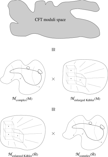
Figure 24: The conformal field theory moduli space.

To summarize the picture of moduli space which has emerged from this discussion, we refer to figure 24. This is the picture which replaces the old and incomplete version of figure 13. The conformal field theory moduli space is geometrically interpretable in terms of the product of a complex structure moduli space and an enlarged Kähler moduli space ${\cal M}_{\rm enlarged~{}K\ddot{a}hler}$. The latter contains numerous complexified Kähler cones of birationally equivalent yet topologically distinct Calabi-Yau manifolds adjoined along common walls. There are two such geometric interpretations, via mirror symmetry, with the roles of complex structure and Kähler structure being interchanged. This is also indicated in figure 24.

We should stress that from an abstract point of view this is a very satisfying picture. As we will discuss more fully in section 10, the augmentation of the Kähler moduli space in the manner presented (and, more precisely, as we will generalize shortly), gives it a mathematical structure which is identical to that of the complex structure moduli space of its mirror. In the important case of Calabi-Yau manifolds which are toric hypersurfaces, both of these moduli spaces are realized as identical compact toric varieties. (The mathematics of toric geometry will be discussed in section 9.) Hence, the picture presented resolves the previous troubling asymmetry between the structure of these two spaces which are predicted to be isomorphic by mirror symmetry.

Although compelling, we have not proven that the picture we are presenting is correct. We have found a natural mathematical structure in algebraic geometry which, if realized by the physics of conformal field theory, resolves some thorny issues in mirror symmetry. We have not established, as yet, whether conformal field theory makes use of this natural mathematical structure. If conformal field theory does avail itself of this structure, though, there is a very precise and concrete conclusion we can draw: every point in the (partially) enlarged Kähler moduli space of $M$ must correspond under mirror symmetry to some point in the complex structure moduli space of $\widetilde{M}$. This implies, of course, that any and all observables calculated in the theories associated to these corresponding points must be identically equal. Let us concentrate on the three-point functions we introduced earlier in (6.6). As we discussed, if we choose a point in the Kähler moduli space for which the instanton corrections are suppressed, the correlation function approaches the topological intersection form on the Calabi-Yau manifold. For ease of calculation, we shall study the correlation functions of (6.28) in this limit. Unlike the analysis of [10], there is not a single unique “large radius” point of the sort we are looking for. Rather, every cell in the (partially) enlarged moduli space supplies us with one such point. Since these cells are the complexified Kähler cones of topologically distinct spaces, the intersection forms associated with these large radius points are different. If the moduli space picture we are presenting in figure 24 is correct, then there must be points in the complex structure moduli space of the mirror whose correlation functions exactly reproduce each and every one of these intersection forms. This is a sharp statement whose veracity would provide a strong verification of the picture presented in figure 24. In the next section we carry out this verification in a particular example.

7.6 An Example

In this section, we briefly carry out the abstract program discussed in the last few sections in a specific example. We will see that the delicate predictions just discussed can be explicitly verified. The mathematics of toric geometry is required to carry out the details of this calculation. As toric geometry can be a bit technical, we shall not discuss it until section 9. Therefore, in this section we shall outline the calculation; some more details will then be given in section 10.3.

We focus on the Calabi-Yau manifold $M$ given by the vanishing locus of a degree $18$ homogeneous polynomial in the weighted projective space $W{\mathbb{C}}P^{4}(6,6$, $3,2,1)$ and its mirror $\widetilde{M}$. For the former we can take the polynomial constraint to be

$$z_{0}^{3}+z_{1}^{3}+z_{2}^{6}+z_{3}^{9}+z_{4}^{18}+a_{0}z_{0}z_{1}z_{2}z_{3}z_{4}=0~{},$$ (7.6)

where the $z_{i}$ are the homogeneous weighted space coordinates and $a_{0}$ is a large and positive constant (whose value, in fact, is inconsequential to the calculations which follow). The mirror to this family of Calabi-Yau spaces is constructed via the method discussed, by taking an orbifold of $M$ by the maximal scaling symmetry group ${\mathbb{Z}}_{3}\times{\mathbb{Z}}_{3}\times{\mathbb{Z}}_{3}$.

A study of the Kähler structure of $M$ reveals that there are five cells in its (partially) enlarged Kähler moduli space, each corresponding to a sigma model on a smooth topologically distinct Calabi-Yau manifold. In each of these cells there is a large radius point for which instanton corrections are suppressed and hence the correlation functions of (6.28) are just the intersection numbers of the respective Calabi-Yau manifolds. These can be calculated for each of the five birationally equivalent, yet topologically distinct, Calabi-Yau spaces and we record the results in table 3. To avoid having to deal with issues associated with normalizing fields in the subsequent discussion, in table 3. we have chosen to list the results in terms of ratios of correlation functions for which such normalizations are irrelevant. (The $D_{i}$ and $H$ are divisors on $M$, corresponding to elements in $H^{1}(M,T^{\star})$ by Poincaré duality.)

Table 3: Ratios of intersection numbers.

   Resolution  $$\Delta_{1} \Delta_{2} \Delta_{3} \Delta_{4} \Delta_{5} {(D_{1}^{3})(D_{4}^{3})\over(D_{1}^{2}D_{4})(D_{1}D_{4}^{2})} -7 0/0 0/0 \infty 9 {(D_{2}^{2}D_{4})(D_{3}^{2}D_{4})\over(D_{2}D_{3}D_{4})(D_{2}D_{3}D_{4})} 2 4 0 0/0 0/0 {(D_{2}D_{3}D_{4})(HD_{2}^{2})\over(D_{2}^{2}D_{4})(HD_{2}D_{3})} 1 1 1 0 0/0 {(D_{2}D_{3}D_{4})(HD_{1}^{2})\over(D_{1}^{2}D_{4})(HD_{2}D_{3})} 2 1 \infty 0/0 0$$                                                                    

Following the discussion of the last section, the goal now is to find five limit points in the complex structure moduli space of $\widetilde{M}$ such that appropriate ratios of correlation functions yield the same results as in table 3. To do so, we note that the most general complex structure on $\widetilde{M}$ can be written

$$W=z_{0}^{3}+z_{1}^{3}+z_{2}^{6}+z_{3}^{9}+z_{4}^{18}+a_{0}\,z_{0}z_{1}z_{2}z_{3}z_{4}+a_{1}z_{2}^{3}z_{4}^{9}+a_{2}z_{3}^{6}z_{4}^{6}+a_{3}\,z_{3}^{3}z_{4}^{12}+a_{4}\,z_{2}^{3}z_{3}^{3}z_{4}^{3}=0~{}.~{}~{}~{}$$ (7.7)

We will describe these limit points by parameterizing the complex structure as $a_{i}=s^{r_{i}}$ for real parameters $s$ and $r_{i}$ and we send $s$ to infinity, the mirror operation of going to large volume. The limit points are therefore distinguished by the rates at which the $a_{i}$ approach infinity. The task, therefore, is to find appropriate values for the $r_{i}$, if they exist, such that we obtain mirrors to the five large radius Calabi-Yau spaces of the last paragraph. The technique we use to do this is to describe both the complex structure moduli space of $\widetilde{M}$ and the enlarged Kähler moduli space of $M$ in terms of toric geometry. This description, as we shall see, makes it manifest that these two moduli spaces are isomorphic. For the present purpose we note that a direct outcome of this analysis — to be covered in section 10.3 — is a prediction for five choices of the vector $(r_{0},\ldots,r_{4})$ which should yield the desired mirrors. As we have discussed, a sensitive test of these predictions is to calculate the mirror of the ratios of correlation functions in table 3 (using (6.27) and the method of [24]) for each of these complex structure limits and see if we get the same answers. This has been done and the results are shown in tables 4 and 5. Note that in the limit $s$ goes to infinity we get precisely the same results. (The $\varphi_{i}$ are elements of $H^{1}(\widetilde{M},T)$.)

Table 4: Asymptotic ratios of 3-point functions.

Resolution	$\Delta_{1}$	$\Delta_{2}$	$\Delta_{3}$
Direction	$({11\over 9},1,{4\over 3},{5\over 3},{5\over 3})$	$({7\over 6},{1\over 2},1,1,{5\over 2})$	$({3\over 2},{1\over 2},2,3,{3\over 2})$
${\langle\varphi_{1}^{3}\rangle\langle\varphi_{4}^{3}\rangle\over\langle\varphi_{1}^{2}\varphi_{4}\rangle\langle\varphi_{1}\varphi_{4}^{2}\rangle}$	$-7-181s^{-1}+\dots$
${\langle\varphi_{2}^{2}\varphi_{4}\rangle\langle\varphi_{3}^{2}\varphi_{4}\rangle\over\langle\varphi_{2}\varphi_{3}\varphi_{4}\rangle\langle\varphi_{2}\varphi_{3}\varphi_{4}\rangle}$	$2-5s^{-1}+\dots$	$4-22s^{-1}+\dots$	$0+2s^{-1}+\dots$
${\langle\varphi_{2}\varphi_{3}\varphi_{4}\rangle\langle\varphi_{0}\varphi_{2}^{2}\rangle\over\langle\varphi_{2}^{2}\varphi_{4}\rangle\langle\varphi_{0}\varphi_{2}\varphi_{3}\rangle}$	$1+{1\over 2}s^{-1}+\dots$	$1+{3\over 2}s^{-2}+\dots$	$1+4s^{-1}+\dots$
${\langle\varphi_{2}\varphi_{3}\varphi_{4}\rangle\langle\varphi_{0}\varphi_{1}^{2}\rangle\over\langle\varphi_{1}^{2}\varphi_{4}\rangle\langle\varphi_{0}\varphi_{2}\varphi_{3}\rangle}$	$2+27s^{-1}+\dots$	$1-{1\over 2}s^{-1}+\dots$	$-2s-33+\dots$

Table 5: Asymptotic ratios of 3-point functions.

Resolution	$\Delta_{4}$	$\Delta_{5}$
Direction	$({13\over 9},2,{5\over 3},{4\over 3},{4\over 3})$	$({11\over 6},{7\over 2},1,1,{3\over 2})$
${\langle\varphi_{1}^{3}\rangle\langle\varphi_{4}^{3}\rangle\over\langle\varphi_{1}^{2}\varphi_{4}\rangle\langle\varphi_{1}\varphi_{4}^{2}\rangle}$	$-{2\over 5}s^{2}-{129\over 250}s+\dots$	$9+289s^{-1}+\dots$
${\langle\varphi_{2}^{2}\varphi_{4}\rangle\langle\varphi_{3}^{2}\varphi_{4}\rangle\over\langle\varphi_{2}\varphi_{3}\varphi_{4}\rangle\langle\varphi_{2}\varphi_{3}\varphi_{4}\rangle}$
${\langle\varphi_{2}\varphi_{3}\varphi_{4}\rangle\langle\varphi_{0}\varphi_{2}^{2}\rangle\over\langle\varphi_{2}^{2}\varphi_{4}\rangle\langle\varphi_{0}\varphi_{2}\varphi_{3}\rangle}$	$0-2s^{-1}+\dots$
${\langle\varphi_{2}\varphi_{3}\varphi_{4}\rangle\langle\varphi_{0}\varphi_{1}^{2}\rangle\over\langle\varphi_{1}^{2}\varphi_{4}\rangle\langle\varphi_{0}\varphi_{2}\varphi_{3}\rangle}$		$0-2s^{-1}+\dots$

This, in conjunction with the abstract and general isomorphism we find between the complex structure moduli space of a Calabi-Yau and the enlarged Kähler moduli space of its mirror, provides us with strong evidence that our understanding of Calabi-Yau conformal field theory moduli space is correct. In particular, as our earlier discussion has emphasized, this implies that the basic operation of deformation by a truly marginal operator (from a space-time point of view, this corresponds to a slow variation in the vacuum expectation value of a scalar field with an exactly flat potential) can result in a change in the topology of the Calabi-Yau target space. This discontinuous mathematical change, however, is perfectly smooth from the point of view of physics. In fact, using mirror symmetry, such an evolution can be reinterpreted as a smooth, topology preserving, change in the “shape” (complex structure) of the mirror space.

There are two important points we need to mention. First, for ease of discussion, we have focused on the case in which the only deformations are those associated with the Kähler structure of $M$ and, correspondingly, only the complex structure of $\widetilde{M}$. This may have given the incorrect impression that the topology changing transitions under study can always be reinterpreted in a topology preserving manner in the mirror description. The generic situation, however, is one in which the complex structure and the Kähler structure of $M$ and $\widetilde{M}$ both change. Again, from a space-time point of view, this simply corresponds to a slow variation of the expectation values of a set of scalar fields with flat potentials. Under such circumstances, topology change can occur in both the original and the mirror description. Our reasoning will ensure that such changes are physically smooth. Clearly there is no interpretation — on the original or on the mirror manifold — which can avoid the topology changing character of the processes.

Second, we have used the terms “enlarged” and “partially enlarged” in our discussion of the Kähler moduli space. We now briefly indicate the distinction. The central result of this discussion is that the proper geometric interpretation of conformal field theory moduli space requires that we augment the previously held notion of a single complexified Kähler cone associated with a single topological type of Calabi-Yau space. In the previous sections, we have focused on part of the requisite augmentation: we need to include the complexified Kähler cones of Calabi-Yau spaces related to the original by flops of rational curves (of course, it is arbitrary as to which Calabi-Yau we call the original). These Kähler cones adjoin each other along common walls. The space so created is the partially enlarged Kähler moduli space. It turns out, though, that conformal field theory moduli space requires that even more regions be added. We saw evidence of this in section 5.3. Equivalently, the partially enlarged Kähler moduli space is only a subregion of the moduli space which is mirror to the complex structure moduli space of the mirror Calabi-Yau manifold. The extra regions which need to be added arise directly from the toric geometric description and were first identified in the two dimensional supersymmetric gauge theory approach of [113], as discussed in section 5.3. These regions correspond to the moduli spaces of conformal theories on orbifolds of the original smooth Calabi-Yau, Landau-Ginzburg orbifolds, gauged Landau-Ginzburg theories and hybrids of the above. The union of all of these regions (which also join along common walls) constitutes the enlarged Kähler moduli space. In section 5.3, the examples we studied only had a single Calabi-Yau region and a single Landau-Ginzburg region. More complicated examples with larger $h^{1,1}$ have richer phase structures. For instance, in the example studied in section 7.6, we found that there were five regions in the partially enlarged Kähler moduli space. The enlarged Kähler moduli space, as it turns out, has $100$ regions. One of these is a Landau-Ginzburg orbifold region, $27$ of these are sigma models on Calabi-Yau orbifolds, and $67$ of these are hybrid theories consisting of Landau-Ginzburg models fibered over various compact spaces. It is worthwhile emphasizing that in contrast with previously held notions, orbifold theories are not simply boundary points in the moduli space of smooth Calabi-Yau sigma models but, rather, they have their own regions in the enlarged Kähler moduli space and hence are more on an equal footing with the smooth examples.

8 Space-Time Topology Change — The Drastic Case

In this section we discuss the results of [67] in which physically smooth transitions between Calabi-Yau manifolds with different Hodge numbers was established. Contrary to the above analysis, non-peturbative effects play a crucial role.

8.1 Basic Ideas

A particularly useful way of summarizing the discussion of the last section is as follows: classical reasoning suggests that our physical models will be badly behaved if the complex structure is chosen to lie on the discriminant locus or if the Kähler class is chosen to lie on a wall of the classical Kähler moduli space. The fully quantum corrected conformal field theory corresponding to such points (yielding genus zero string theory), though, proves to be generically non-singular on walls in the Kähler moduli space. The pronounced distinction between the classical and stringy conclusions arises because such points are strongly coupled theories (as the coupling parameter $\alpha^{\prime}/R^{2}$ gets big as we shrink down $R$ — the radius of an $S^{2}$). Analyzing such strongly coupled theories directly is hard; however, by mirror symmetry we know they are equivalent to weakly coupled field theories on the mirror Calabi-Yau space where we can directly show them to be well behaved.

So much for the generic point on a wall in the Kähler parameter space: classically they look singular but in fact they are well defined. What about choosing the complex structure to lie on the discriminant locus (which by mirror symmetry corresponds to a non-generic point on a wall in the Kähler parameter space of the mirror)? Might it be that these theories are well behaved too? At first sight the answer seems to be “no”. By taking the Kähler class to be deep inside a smooth phase (i.e. a smooth large radius Calabi-Yau background), we trust perturbation theory and can directly compute conformal field theory correlation functions. Some of them diverge as we approach the discriminant locus. This establishes that the conformal field theory is badly behaved. It is, however, important to distinguish between conformal field theory and string theory. Conformal field theory is best thought of as the effective description of string degrees of freedom which are light in the $g_{s}\rightarrow 0$ limit, with $g_{s}$ being the string coupling constant. This includes all of the familiar perturbative string states, but effectively integrates out non-perturbative states whose most direct description is in terms of solitons in the low energy effective string action. As discussed in [95] a powerful microscopic way of describing these states is in in terms of Dirichlet-branes. For the most part of our discussion, the details of such a description will not be essential.

We are thus faced with the moduli space for an effective string description that contains points where physics appears to be singular. A close analog of this situation plays a central role in the celebrated work of Seiberg and Witten [102], where it is argued that the apparent singularity is due to the appearance of new massless non-perturbative degrees of freedom at those singular moduli space points. A natural guess in the present setting, then, is that the apparent singularity encountered on the discriminant locus is due to previously massive non-perturbative string states becoming massless. This solution was proposed by Strominger and we review its success in the next section.

8.2 Strominger’s Resolution of the Conifold Singularity

To quantitatively understand the proposed resolution of conifold singularities, we must introduce coordinates on the complex structure moduli space. A convenient way to do this — described in some detail in [28] — is to introduce a symplectic homology basis of $H^{3}(M,{\mathbb{Z}})$. This means that we find three-cycle representatives in $H^{3}(M,{\mathbb{Z}})$. denoted by $\{A_{I},B^{J}\}$, where $I,J=0,...,h^{2,1}(M)$ such that

$$A_{I}\cap B^{J}=\delta_{I}^{J}~{},~{}~{}~{}A_{I}\cap A_{J}=B^{I}\cap B^{J}=0~{}.$$

As we wander around the complex structure moduli space, the holomorphic three-form will vary, and we can use this variation as a means of establishing local coordinates. To do so, we let

$$z^{J}\equiv\int_{B^{J}}\Omega~{},$$ (8.8)

and

$$G_{I}=\int_{A^{I}}\Omega~{},$$ (8.9)

where $\Omega$, as usual, is the holomorphically varying three-form on the family of Calabi-Yau spaces being studied. It is well known that the $z^{J}$ provide a good set of local projective coordinates on the moduli space of complex structures and that the $G_{I}$ can be expressed as functions of the $z^{J}$.

In terms of these coordinates, a conifold point in the moduli space can roughly be thought of as a point where some $z^{J}$’s vanishes (we will be more precise on this in the next section). The corresponding $B^{J}$ is called a vanishing cycle as the period of $\Omega$ over it goes to zero. Intuitively, this homology cycle is collapsing as we approach the point $z^{J}=0$ in the moduli space. For our purposes, there is one main implication of the vanishing of, say, $z^{J}$, that we should discuss: the metric on the moduli space is singular at such a point. The easiest way to see this is to make use of the fact that the moduli space geometry of Calabi-Yau manifolds is highly constrained. Not only is the complex structure moduli space (and the Kähler moduli space as well) a Kähler manifold in its own right, it is actually a special Kähler manifold. We recall from section 2.12 that special Kähler manifolds have the property that there is a holomorphic potential $\cal F$ for the Kähler potential, called the prepotential. Letting $G_{J}=\partial{\cal F}/\partial z^{J}$, the Kähler potential on the on the complex structure moduli space can be written

$$K=-\ln(i\,{\overline{z}}^{I}\,G_{I}-i\,z^{I}\,{\overline{G}}_{I})~{}.$$ (8.10)

If we knew the explicit form for $G_{J}(z)$, we would thus be able to calculate the local form of the metric near the conifold point. Considerations of monodromy are sufficient to do this: as we will discuss in greater generality below, if we follow a path in the moduli space that encircles $z^{J}=0$, the period $G_{J}$ is not single-valued but rather undergoes a non-trivial monodromy transformation

$$G_{J}\rightarrow G_{J}+z^{J}~{}.$$ (8.11)

Near $z^{J}=0$, we can therefore write

$$G_{J}(z^{J})={1\over 2\pi i}\,z^{J}\ln z^{J}+\hbox{\rm single-valued}~{}.$$ (8.12)

Using this form one can directly compute that the metric $g_{J\overline{J}}$ has a curvature singularity at $z^{J}=0$.

The reason that the singularity of the metric on the moduli space is an important fact is due to its appearance in the Lagrangian for the four-dimensional effective description of the moduli for a string model built on such a Calabi-Yau. Namely, the (space-time) non-linear sigma model Lagrangian for the complex structure moduli $\phi^{K}$ is of the form

$$\int\,d^{4}x\,g_{I\overline{J}}\,\nabla\phi^{I}\,\nabla\phi^{\overline{J}}~{}.$$

Hence, when the metric on the moduli space degenerates, so apparently does our physical description.

This circumstance — a moduli space of theories containing points at which physical singularities appear to develop — is one that has been discussed extensively in recent work of Seiberg and Witten [102]. The natural explanation advanced for the physical origin of the singularities encountered is that states which are massive at generic points in the moduli space become massless at the singular points. As the Lagrangian description is that of an effective field theory in which massive degrees of freedom have been integrated out, if a previously massive degree of freedom becomes massless, then we will be incorrectly integrating out a massless mode and hence expect a singularity to develop. In the case studied in [102], the states that became massless were BPS saturated magnetic monopoles or dyons. Strominger proposed that in compactified type IIB string theory there are analogous electrically or magnetically charged black hole states that become massless at conifold points. The easiest way to understand these states is to recall that, in ten-dimensional type IIB string theory, there are $3+1$ dimensional extremally charged extended soliton solutions with a horizon: so-called black three-branes [72]. These solitons carry Ramond-Ramond charge that can be detected by integrating the five-form field strength over a surrounding Gaussian five-cycle $\Sigma_{5}$:

$$Q_{\Sigma_{5}}=\int_{\Sigma_{5}}F^{(5)}~{}.$$

Now, our real interest is in how this soliton appears after compactification to four dimensions via a Calabi-Yau three-fold. Upon such compactification, the three spatial dimensions of the black soliton can wrap around non-trivial three-cycles on the Calabi-Yau and hence appear to a four-dimensional observer as black hole states. More precisely, they yield an $N=2$ hypermultiplet of states. The effective electric and magnetic charges of the black hole state are then obtained by integrating $F^{(5)}$ over $A_{I}\times S^{2}$ and $B^{J}\times S^{2}$. Explicitly, making the natural assumption of charge quantization, we can write

$$\int_{A_{I}\times S^{2}}F^{(5)}=g_{5}\,n_{I}~{},~{}~{}~{}~{}~{}\int_{B^{J}\times S^{2}}F^{(5)}=g_{5}\,m^{J}~{},$$ (8.13)

where $g_{5}$ is the five-form coupling and $n_{I}$, $m_{J}$ are some integers. Of prime importance is the fact that these are BPS saturated states and hence are subject to the mass relation [32]

$$M=g_{5}\,e^{K/2}\,|m^{I}\,G_{I}-n_{I}\,z^{I}|~{}.$$ (8.14)

Let us consider the case in which $n_{I}$ = $\delta_{IJ}$ and $m^{I}=0$, for all $I$ with $J$ fixed. In the conifold limit for which $z^{J}$ goes to zero, we see that the mass of the corresponding electrically charged black hole vanishes. Hence, it is no longer consistent to exclude such states from direct representation in the Wilsonian effective field theory action describing the low energy string dynamics.

The claim is that the singularity encountered above is due precisely to such exclusion. Curing the singularity should therefore be achieved by a simple procedure: include the black hole hypermultiplet in the low energy effective action. There is a simple check to test the validity of this claim. Namely, if we incorrectly integrate out the black hole hypermultiplet from the Wilsonian action, we should recover the singularity discussed above. This is not hard to do. The structure of $N=2$ space-time supersymmetry implies that the effective Lagrangian is governed by a geometrical framework which is identical to that governing Calabi-Yau moduli space. Namely, we can introduce holomorphic projective coordinates $z^{J}$ on the moduli space of the physical model; the model is determined by knowledge of the holomorphic functions $G^{\rm phys}_{I}(z)$ which are in turn determined by a holomorphic prepotential ${\cal F}^{\rm phys}$. The superscript “phys” is meant to distinguish these objects from their geometric counterparts, although we show momentarily see that they are identical. The Lagrangian for an $N=2$ space-time theory can be written in a manifestly supersymmetric form as

$${\cal L}={1\over 8\pi}\,\,{\rm Im}\left[\int d^{2}\theta\,\tau_{IJ}\,W^{I\alpha}W^{J}_{\alpha}+\dots\right]~{},$$ (8.15)

where

$$\tau_{IJ}=\partial_{I}G^{\rm phys}_{J}~{}.$$

and $W^{I}$ are certain superfields. Therefore, the coupling constant for the $J$-th $U(1)$ is given by

$$\tau_{JJ}=\partial_{J}G^{\rm phys}_{J}~{}.$$

We can turn the latter statement around by noting that knowledge of the coupling constant effectively allows us to determine $G_{J}$. We can determine the behaviour of the coupling by a simple one-loop Feynman diagram, which again by $N=2$ is all we need consider. Integrating out a black hole hypermultiplet in a neighborhood of the $z^{J}=0$ conifold point yields the standard logarithmic contribution to the running coupling $\tau_{JJ}$ and hence we can write

$$\tau_{JJ}={{1\over 2\pi i}}\ln z^{J}+\hbox{\rm single-valued}~{}.$$ (8.16)

From this we determine, by integration, that

$$G^{\rm phys}_{J}={{1\over 2\pi i}}z^{J}\ln z^{J}+\hbox{\rm single-valued}~{}.$$ (8.17)

We note that this is precisely the same form as we found for $G_{J}$ earlier via mathematical monodromy considerations. Now, by special geometry, everything about the mathematics and physics of the system follows from knowledge of the $G_{J}$. The Kähler potential and hence metric on the moduli space are determined by (2.77). For our purposes, therefore, the singularity encountered previously (by determining the metric on the moduli space from the $G_{J}$), has been precisely reproduced by incorrectly integrating out the massless soliton state. This justifies the claim, therefore, that we have identified the physical origin of the singularity and also that by including the black hole field in the Wilsonian action (and therefore not making the mistake of integrating them out when they are light), we cure the singularity.

8.3 Conifold Transitions and Topology Change

In the previous section, we have seen how the singularity that arises when an $S^{3}$ collapses to a point is associated with the appearance of new massless states in the physical spectrum. By including these new massless states in the physical model, the singularity is cured. In this section, we consider a simple generalization of this discussion which leads to dramatic new physical consequences [67]. Concretely, we consider a less generic degeneration in which:

1. More than one, say $P$, three-cycles degenerate.

2. These $P$ three-cycles are not homologically independent but rather satisfy $R$ homology relations.

As we will now discuss, this generalization implies that:

1. The bosonic potential for the scalar fields in the hypermultiplets that become massless at the degeneration has $R$ flat directions.

2. Moving along such flat directions takes us to another branch of type II string moduli space, corresponding to string propagation on a topologically distinct Calabi-Yau manifold. If the original Calabi-Yau has Hodge numbers $h^{1,1}$ and $h^{2,1}$ then the new Calabi-Yau has Hodge numbers $h^{1,1}+R$ and $h^{2,1}-P+R$.

In order to understand this result, there are a couple of useful pieces of background information we should review. First, let us discuss a bit more precisely the mathematical singularities we are considering [81]. As we have discussed, the discriminant locus denotes those points in the complex structure moduli space of a Calabi-Yau where the space fails to be a complex manifold. We focus on cases in which the degenerations occur at some number of isolated points on the Calabi-Yau. In particular, we consider singularities that are known as “ordinary double points”. These are singular points which can locally be expressed in the form

$$\sum_{i=1}^{4}w_{i}^{2}=0$$ (8.18)

in ${\mathbb{C}}^{4}$. This local representation is a cone with singular point at the apex, namely the origin. To identify the base of the cone we intersect it with a seven-sphere in ${\mathbb{R}}^{8}$,

$$\sum_{i=1}^{4}|w_{i}|^{2}=r^{2}~{}.$$

Introducing the complex vector $\vec{w}=\vec{x}+i\vec{y}=(w_{1},w_{2},w_{3},w_{4})$ the equation of the intersection can be expressed as

$$\vec{x}\cdot\vec{x}={r^{2}\over 2}~{},~{}~{}~{}~{}~{}\vec{y}\cdot\vec{y}={r^{2}\over 2}~{},~{}~{}~{}~{}~{}\vec{x}\cdot\vec{y}=0~{}.$$

The first of these is an $S^{3}$, the latter two equations give an $S^{2}$ fibered over the $S^{3}$. As there are no non-trivial such fibrations, the base of the cone is $S^{2}\times S^{3}$. Calabi-Yau spaces which have such isolated ordinary double point singularities are known as conifolds and the corresponding point in the moduli space of the Calabi-Yau is known as a conifold point. The ordinary double point singularity is also referred to as a node. In figure 25 we illustrate a neighbourhood of a node.

Figure 25: The neighbourhood around a node.

Having described the singularity in this way we immediately discern two distinct ways of resolving it: either we can replace the apex of the cone with an $S^{3}$, known as a deformation of the singularity, or we can replace the apex with an $S^{2}$, known as a small resolution of the singularity. These two possibilities are illustrated in figure 26. The deformation simply undoes the degeneration by re-inflating the shrunken $S^{3}$ to positive size. The small resolution, on the other hand, has a more pronounced effect: it repairs the singularity in a manner that changes the topology of the original Calabi-Yau. After all, replacing an $S^{3}$ with an $S^{2}$ is a fairly radical transformation. We shall find the physical interpretation of these two ways of resolving conifold singularities.

Figure 26: The two possible resolutions of a node.

A second piece of background information is a mathematical fact due to Lefshetz concerning monodromy. Namely, if $\gamma^{a}$ for $a=1,...,k$ are $k$ vanishing three-cycles at a conifold point in the moduli space, then another three-cycle $\delta$ undergoes monodromy

$$\delta\rightarrow\delta+\sum_{a=1}^{k}\,(\delta\cap\gamma^{a})\,\gamma^{a}$$ (8.19)

upon transport around this point in the moduli space.

With this background, we can now proceed to discuss the result quoted at the beginning of this section. We will do so in the context of a particularly instructive example, although it will be clear that the results are general. We begin with the quintic hypersurface in ${\mathbb{C}}P^{4}$, which is we have seen to have Hodge numbers $h^{2,1}=101$ and $h^{1,1}=1$. We then move to a conifold point by deforming the complex structure to the equation

$$x_{1}\,g(x)+x_{2}\,h(x)=0~{},$$ (8.20)

where $x$ denotes the five homogeneous ${\mathbb{C}}P^{4}$ coordinates $(x_{1},...,x_{5})$ and $g$ and $h$ are both generic quartics. We note that (8.20) and its derivative vanish at the sixteen points

$$x_{1}=x_{2}=g(x)=h(x)=0~{}.$$ (8.21)

It is straightforward to check, by examining the second derivative matrix, that for generic $g$ and $h$ these are sixteen ordinary double points. And, of primary importance to our present discussion, the sixteen singular points lie on the ${\mathbb{C}}P^{2}$ contained in ${\mathbb{C}}P^{4}$ given by $x_{1}=x_{2}=0$. This implies that the sixteen vanishing cycles $\gamma^{a},a=1,...,16$ that degenerate to the double points satisfy the non-trivial homology relation [35]

$$\sum_{a=1}^{16}\,\gamma^{a}=0~{}.$$ (8.22)

We are thus in the desired situation. To proceed with the physical analysis, we follow two steps. First, we check that inclusion of the appropriate massless hypermultiplets cures the singularity, as it did in the simpler case studied in [106]. Second, we analyze the physical implication of the existence of a non-trivial homology relation.

i) Singularity resolution:

We introduce a symplectic homology basis $\{A_{I},B^{J}\}$, with $I,J=1,...,204$. By suitable change of basis we can take our sixteen vanishing cycles $\gamma^{a}$ $(a=1,...,16)$ to be $B^{1},...,B^{15}$ and $-\sum_{a=1}^{15}B^{a}$. As usual, we define

$$z^{I}=\int_{B^{I}}\Omega~{},~{}~{}~{}~{}~{}G_{J}=\int_{A_{J}}\Omega~{}.$$

Now, for any cycle $\delta$ we have, as discussed before, the monodromy

$$\delta\rightarrow\delta+\sum_{a=1}^{16}\,(\delta\cap\gamma^{a})\,\gamma^{a}~{}.$$

From this we learn that the local form of the period over $\delta$ is given by

$$\int_{\delta}\Omega={1\over 2\pi i}\,\sum_{a=1}^{16}(\delta\cap\gamma^{a})\,(\int_{\gamma^{a}}\Omega)\,(\ln\int_{\gamma^{a}}\Omega)+\hbox{\rm single-valued}~{}.$$ (8.23)

Specializing this general expression to $\delta=A_{J}$, we therefore see

$$G_{J}={1\over 2\pi i}\,z^{J}\ln z^{J}+{1\over 2\pi i}\,(\sum_{I=1}^{15}z^{I})\,(\ln\sum_{I=1}^{15}z^{I})+\hbox{\rm single-valued}~{}.$$ (8.24)

By special geometry, this latter expression determines the properties of the singularity associated with the conifold degeneration being studied. Thus, the question we now seek to answer is: if we incorrectly integrate out the black hole states which become massless at this conifold point, do we reproduce the form (8.24)?

To address this issue we must identify the precise number and charges of the states that are becoming massless at the degeneration point. As discussed in [106], the counting of black hole states is a delicate issue for which there is as yet no rigorous algorithm. In [106], one homology class in $H^{3}$ degenerated at the conifold singularity and it was hypothesized that this implies one fundamental black hole state — the one of minimal charge — needs to be included in the Wilsonian action. In the present example, though, we have sixteen three cycles in fifteen homology classes in $H^{3}$ degenerating. In [67] it was argued that this should imply sixteen fundamental black hole fields need to be included in the Wilsonian action. Physically speaking, the black three-brane can wrap around any of the sixteen degenerating three-cycles, which at large overall radius of the Calabi-Yau would be widely separated. It thus seems sensible that even though there are only fifteen homology classes degenerating, we actually get sixteen massless black hole states. Subsequent analyses by [19, 94] have shown that one expects a massless hypermultiplet for each supersymmetric three-cycle in a given degenerating homology class. It can be a subtle undertaking to find all such supersymmetric cycles, but the physical reasoning given above for the example at hand is quite convincing, so we will pursue the implications of having sixteen new massless hypermultiplets.

The charges of these states are easy to derive. If we let $H^{a}$ be the black hole hypermultiplet associated with the vanishing cycle $\gamma^{a}$ then the charge of $H^{a}$ under the $I$-th $U(1)$ is given by

$$Q^{a}_{I}=A_{I}\cap\gamma^{a}~{},$$

where we write $F^{(5)}$ as the self-dual part of $\sum_{I}\alpha^{I}F_{I}^{(2)}$, with $\alpha^{I}$ dual to $A_{I}$. We immediately learn from this that the black holes states have charges

$$Q^{a}_{I}=\delta^{a}_{I}~{},~{}~{}~{}1\leq a\leq 15\quad\hbox{ \rm and }\quad Q^{16}_{I}=-1,~{}~{}~{}1\leq I\leq 15~{},$$ (8.25)

with all other charges zero. This is enough data to determine the running of the gauge couplings:

$$\tau_{IJ}={{1\over 2\pi i}}\sum_{a=1}^{16}\,Q^{a}_{I}\,Q^{a}_{J}\,\ln m^{a}~{},$$ (8.26)

where the mass $m^{a}$ of $H^{a}$ is proportional to $\sum_{I}Q^{a}_{I}z^{I}.$ Using the above charges we therefore have

$$\tau_{IJ}={1\over 2\pi i}\delta_{IJ}\,\ln z^{J}+{{1\over 2\pi i}}\,\ln\sum_{k=1}^{15}z^{k}+\hbox{\rm single-valued}~{}.$$ (8.27)

Integrating we find therefore

$$G_{J}^{\rm phys}={{1\over 2\pi i}}z^{J}\,\ln z^{J}+{{1\over 2\pi i}}(\sum_{k=1}^{15}z^{k})\,(\ln\sum_{k=1}^{15}z^{k})+\hbox{\rm single-valued}~{}.$$ (8.28)

We note that this matches (8.24) and hence we have shown that inclusion of the sixteen black hole soliton states which become massless cures the singularity.

Having shown that a slight variant on Strominger’s original proposal is able to cure the singularity found in this more complicated situation, we now come to the main point of the discussion:

ii) What is the physical significance of non-trivial homology relations between vanishing cycles?

To address this question we consider the scalar potential governing the black hole hypermultiplets. It can be written as [110]:

$$V=\sum\,E^{I}_{\alpha\beta}\,E^{\alpha\beta}_{I}~{},$$ (8.29)

where

$$E^{I}_{\alpha\beta}=\sum_{a=1}^{16}\,Q^{I}_{a}\,\epsilon_{\alpha\gamma}h^{*(a)}_{\gamma}\,h^{(a)}_{\beta}-(\alpha\leftrightarrow\beta)~{},$$ (8.30)

in which the indices satisfy $I=1,...,15,~{}\alpha,\beta,\gamma=1,2$. The fields $h^{(a)}_{1}$ and $h^{(a)}_{2}$ are the two complex scalar fields in the hypermultiplet $H^{a}$.

We consider the possible flat directions which this potential admits. The most obvious flat directions are those for which $\langle h^{(a)}_{\beta}\rangle=0$ with non-zero values for the scalar fields in the vector multiplets. Physically, moving along such flat directions takes us back to the Coulomb phase in which the black hole states are massive. Mathematically, moving along such flat directions,

$${1\over 2\pi i}\,(\sum_{k=1}^{15}z^{k})\,\ln\sum_{k=1}^{15}z^{k}$$ (8.31)

gives positive volume back to the degenerated $S^{3}$’s and hence resolves the singularity by deformation.

The non-trivial homology relation implies that there is another flat direction. Since $Q^{I}_{a}=A_{I}\cap\gamma^{a}$, we see that the homology relation $\sum_{a=1}^{16}\gamma^{a}=0$ implies $\sum_{a}Q^{I}_{a}=0$, for all $I$. This then implies that we have another flat direction of the form $\langle h^{(a)}_{\beta}\rangle=v^{\beta}$ for all $a$ with $v$ constant. In fact, simply counting degrees of freedom shows that this solution is unique up to gauge equivalence. What happens if we move along this flat direction? It is straightforward to see that this takes us to a Higgs branch in which fifteen vector multiplets pair up with fifteen hypermultiplets to become massive. This leaves over one massless hypermultiplet from the original sixteen that become massless at the conifold point. We see therefore that the spectrum of the theory goes from $101$ vector multiplets and $1$ hypermultiplet (ignoring the dilaton and graviphoton) to $101-15=86$ vector multiplets and $1+1=2$ hypermultiplets.

What is the significance of these numbers? Well, it turns out [25, 26] that precisely these Hodge numbers arise from performing the other resolution of the conifold singularity (besides the deformation) — the small resolution described earlier! Hence, we appear to have found the physical mechanism for effecting a small resolution and in this manner changing the topology of the Calabi-Yau background.

Although we have focused on a specific example, it is straightforward to work out what happens in the more general setting of $P$ isolated vanishing cycles satisfying $R$ homology relations. Following our discussion above, we get $P$ black hole hypermultiplets becoming massless with $R$ flat directions in their scalar potential. Performing a generic deformation along these flat directions causes $P-R$ vectors to pair up with the same number of hypermultiplets. Hence the Hodge numbers change according to

$$(h^{2,1},h^{1,1})\rightarrow(h^{2,1}-(P-R),h^{1,1}+R)~{}.$$ (8.32)

The Euler characteristic of the variety thus jumps by $2P$.

So, in answer to the question posed above: homology relations amongst the vanishing cycles give rise to new flat directions in the scalar black hole potential. Moving along such flat directions takes us smoothly to new branches of the type II string theory moduli space. These other branches correspond to string propagation on topologically distinct Calabi-Yau manifolds. We have therefore apparently physically realized the Calabi-Yau conifold transitions discussed some years ago — without a physical mechanism — in insightful papers of Candelas, Green and Hübsch [25, 26]. In the type II string moduli space we thus see that we can smoothly go from one Calabi-Yau manifold to another by varying the expectation values of appropriate scalar fields.

8.4 Black Holes, Elementary Particles and a New Length Scale

There are two other aspects of these topology changing transitions which are worthy of emphasis. First, in the Coulomb phase, the black hole soliton states are massive. At the conifold point they become massless. As we move into the Higgs phase, some number of them are eaten by the Higgs mechanism with the remainder staying massless. Now, with respect to the topology of the new Calabi-Yau in the Higgs phase, these massless degrees of freedom are associated with new elements of $H^{1,1}$. Such states, as is well known, are perturbative string excitations — commonly referred to as elementary “particles”. Thus, a massive black hole sheds its mass, becomes massless and then re-emerges as an elementary particle-like excitation. There is thus no invariant distinction between black hole states and elementary perturbative string states: they smoothly transform into one another through the conifold transitions. This realizes an old suspicion linking black holes and elementary particles in a quite explicit manner.

The second point we wish to emphasize is one made in [101] and discussed in Shenker’s lectures of this school. Let us consider a bit more carefully the origin of the logarithmic running in (8.16). We have a charged black hole hypermultiplet of mass (putting all of the couplings in place):

$$m_{\rm bh}\sim|z|m_{s}/g_{s}~{},$$

where $m_{s}\sim 1/\sqrt{\alpha^{\prime}}$. The one-loop charge screening interaction therefore contributes

$$\int^{\Lambda}{d^{4}k\over(2\pi)^{4}}\,{1\over k^{2}+m_{b}h^{2}}\sim-\ln{\Lambda\over m_{\rm bh}}~{},$$ (8.33)

where $\Lambda$ is the ultraviolet scale above which an effective description in terms of a point-like black hole state is no longer accurate. At first sight, one’s natural guess is that $\Lambda$ should be on the order of $m_{s}$ since above this energy scale we expect the extended nature of the string to have a dominant effect. An examination of (8.33) reveals that this expectation does not appear to be correct. Rather, in order for (8.33) to be $g_{s}$ independent (as it must by the decoupling of vector multiplets and neutral hypermultiplets like the dilaton), we see that $\Lambda\sim m_{s}/g_{s}$, so that (8.33) gives the desired $\ln z$ behavior. In other words, the point-like description of these solitons persists all the way down to length scales of order $g_{s}\sqrt{\alpha^{\prime}}$. For small string coupling, this is much less than the previous conception of the string scale setting a “lower” length limit to physical processes. Study of such non-perturbative string degrees of freedom thus reveals the possibility of a whole new sub-string scale geometrical world — a realm that is presently under instense study.

9 The Basics of Toric Geometry

Toric geometry has played an important role in a number of developments in quantum geometry. Projective and weighted projective spaces are examples of toric varieties and hence a huge number of Calabi-Yau manifolds can be realized as subspaces of toric varieties. As we shall see, the toric structure provides a systematic framework for understanding detailed properties of Calabi-Yau manifolds constructed in this manner. Our goal in this chapter is to give an elementary discussion of toric geometry emphasizing those points most relevant to the present lectures. For more details and proofs the reader should consult [91, 49]. We will then apply this formalism to better understand some of the details of flop transitions discussed earlier as well as to extend and generalize the conifold transitions of the last chapter.

9.1 Intuitive Ideas

Toric geometry describes the structure of a certain class of geometrical spaces in terms of simple combinatorial data. When a space admits a description in terms of toric geometry, many basic and essential characteristics of the space — such as its divisor classes, its intersection form and other aspects of its cohomology — are neatly coded and easily deciphered from analysis of corresponding lattices. We will describe this more formally in the following subsections. Here we outline the basic ideas.

The complex projective space ${\mathbb{C}}P^{n}$ can be expressed as

$${\mathbb{C}}P^{n}={{\mathbb{C}}^{n+1}-\{0,0,...,0\}\over{\mathbb{C}}^{*}}~{},$$ (9.34)

where the ${\mathbb{C}}^{*}$ action by which we quotient is $(z_{1},...,z_{n+1})\rightarrow(\lambda z_{1},...,\lambda z_{n+1})$. A toric variety is a generalization of this in which rather than just removing the origin, we remove a point set $F_{\Delta}$ depending on certain data $\Delta$ and we quotient by a number of ${\mathbb{C}}^{*}$ actions. That is, a toric variety $V$ can be expressed in the form

$$V={{\mathbb{C}}^{m}-F_{\Delta}\over({\mathbb{C}}^{*})^{p}}~{}.$$ (9.35)

As we shall see in the sequel, the action of $({\mathbb{C}}^{*})^{p}$ and the form of $F_{\Delta}$ will be determined in terms of certain simple combinatorial data. In building up to this description, it is worthwile to recall another feature of ${\mathbb{C}}P^{n}$: it contains $({\mathbb{C}}^{*})^{n}$ as a dense open subset and can therefore be thought of as a compactification of $({\mathbb{C}}^{*})^{n}$. To keep a concrete example in mind, ${\mathbb{C}}P^{1}$ is nothing but the sphere $S^{2}$. The latter is a compactification of ${\mathbb{C}}^{*}$ in which we add the points at zero and infinity. These points, in fact, can be thought of as limiting points of the natural action of ${\mathbb{C}}^{*}$ on itself. In general, this gives another way of thinking about toric varieties: partial or complete compactifications of products of ${\mathbb{C}}^{*}$ where the boundary points included are derived from limits of an action of the ${\mathbb{C}}^{*}$ factors on themselves. We will begin with this perspective.

Following the above remarks, a toric variety $V$ over ${\mathbb{C}}$ (one can work over other fields but that shall not concern us here) is a complex geometrical space which contains the algebraic torus

$$T=\underbrace{{\mathbb{C}}^{*}\times\ldots\times{\mathbb{C}}^{*}}_{n}\cong({\mathbb{C}}^{*})^{n}$$

as a dense open subset. Furthermore, there is an action of $T$ on $V$; that is, a map $T\times V\rightarrow V$ which extends the natural action of $T$ on itself. The points in $V-T$ can be regarded as limit points for the action of $T$ on itself; these serve to give a partial compactification of $T$. Thus, $V$ can be thought of as a $({\mathbb{C}}^{*})^{n}$ together with additional limit points which serve to partially (or completely) compactify the space. Different toric varieties, therefore, are distinguished by their different compactifying sets. The latter, in turn, are distinguished by restricting the limits of the allowed action of $T$ and these restrictions can be encoded in a convenient combinatorial structure as we now describe.

In the framework of an action $T\times V\rightarrow V$, we can focus our attention on one-parameter subgroups of the full $T$ action. Basically, we follow all possible holomorphic curves in $T$ as they act on $V$ and ask whether or not the action has a limit point in $V$. As the algebraic torus $T$ is a commutative algebraic group, all of its one-parameter subgroups are labeled by points in a lattice $N\cong{\mathbb{Z}}^{n}$ in the following way. Given $(n_{1},\ldots,n_{n})\in{\mathbb{Z}}^{n}$ and $\lambda\in{\mathbb{C}}^{*}$, we consider the one-parameter group ${\mathbb{C}}^{*}$ acting on $V$ by

$$\lambda\cdot(z_{1},\ldots,z_{n})\rightarrow(\lambda^{n_{1}}z_{1},\ldots,\lambda^{n_{n}}z_{n})~{},$$ (9.36)

where $(z_{1},\ldots,z_{n})$ are local holomorphic coordinates on $V$ (which may be thought of as residing in the open dense $({\mathbb{C}}^{*})^{n}$ subset of $V$). Now, to describe all of $V$ (that is, in addition to $T$) we consider the action of (9.36) in the limit that $\lambda$ approaches zero (and thus moves from ${\mathbb{C}}^{*}$ into ${\mathbb{C}}$). It is these limit points which supply the partial compactifications of $T$ thereby yielding the toric variety $V$. The limit points obtained from the action (9.36) depend upon the explicit vector of exponents $(n_{1},\ldots,n_{n})\in{\mathbb{Z}}^{n}$, but many different exponent vectors can give rise to the same limit point. We obtain different toric varieties by imposing different restrictions on the allowed choices of $(n_{1},\ldots,n_{n})$ and by grouping them together (according to common limit points) in different ways.

We can describe these restrictions and groupings in terms of a “fan” $\Delta$ in $N$ which is a collection of strongly convex rational polyhedral cones $\sigma_{i}$ in the real vector space $N_{{\mathbb{R}}}=N\otimes_{{\mathbb{Z}}}{\mathbb{R}}$. (In simpler language, each $\sigma_{i}$ is a convex cone with apex at the origin spanned by a finite number of vectors which live in the lattice $N$ and such that any angle subtended by these vectors at the apex is less than $180^{\circ}$.) The fan $\Delta$ is a collection of such cones which satisfy the requirement that the face of any cone in $\Delta$ is also in $\Delta$. Now, in constructing $V$, we associate a coordinate patch of $V$ to each large cone $\sigma_{i}$ in $\Delta$, where large refers to a cone spanning an $n$-dimensional subspace of $N$. This patch consists of $({\mathbb{C}}^{*})^{n}$ together with all the limit points of the action (9.36) for $(n_{1},\ldots,n_{n})$ restricted to lie in $\sigma_{i}\cap N$. There is a single point which serves as the common limit point for all one-parameter group actions with vector of exponents $(n_{1},\ldots,n_{n})$ lying in the interior of $\sigma_{i}$; for exponent vectors on the boundary of $\sigma_{i}$, additional families of limit points must be adjoined.

We glue these patches together in a manner dictated by the precise way in which the cones $\sigma_{i}$ adjoin each other in the collection $\Delta$. Basically, the patches are glued together in a manner such that the one-parameter group actions in the two patches agree along the common faces of the two cones in $\Delta$. We will be more precise on this point shortly. The toric variety $V$ is therefore completely determined by the combinatorial data of $\Delta$.

Figure 27: A simple fan.

For a simple illustration of these ideas, consider the two-dimensional example of $\Delta$ shown in 27. As $\Delta$ consists of two large cones, $V$ contains two coordinate patches. The first patch — corresponding to the cone $\sigma_{1}$ — represents $({\mathbb{C}}^{*})^{2}$ together with all limit points of the action

$$\lambda\cdot(z_{1},z_{2})\rightarrow(\lambda^{n_{1}}z_{1},\lambda^{n_{2}}z_{2})~{},$$ (9.37)

with $n_{1}$ and $n_{2}$ non-negative as $\lambda$ goes to zero. We add the single point $(0,0)$ as the limit point when $n_{1}>0$ and $n_{2}>0$; we add points of the form $(z_{1},0)$ as limit points when $n_{1}=0$ and $n_{2}>0$; we finally add the points of the form $(0,z_{2})$ as limit points when $n_{1}>0$ and $n_{2}=0$.

Clearly, this patch corresponds to ${\mathbb{C}}^{2}$. By symmetry, we also associate a ${\mathbb{C}}^{2}$ with the cone $\sigma_{2}$. Now, these two copies of ${\mathbb{C}}^{2}$ are glued together in a manner dictated by the way $\sigma_{1}$ and $\sigma_{2}$ adjoin each other. Explaining this requires that we introduce some more formal machinery to which we now turn.

9.2 The $M$ and $N$ Lattices

In the previous subsection, we have seen how a fan $\Delta$ in $N_{{\mathbb{R}}}$ serves to define a toric variety $V$. The goal of this subsection is to make the connection between lattice data and $V$ more explicit by showing how to derive the transition functions between the patches of $V$. The first part of our presentation will be in the form of an algorithm that answers the question: given the fan $\Delta$ how do we explicitly define coordinate patches and transition functions for the toric variety $V$? We will then briefly describe the mathematics underlying the algorithm.

Towards this end, it proves worthwhile to introduce a second lattice defined as the dual lattice to $N$, $M=\mathop{\rm Hom}(N,{\mathbb{Z}})$, where $\mathop{\rm Hom}$ denotes homomorphism. We denote the dual pairing of $M$ and $N$ by $\langle~{},~{}\rangle$. Corresponding to the fan $\Delta$ in $N_{{\mathbb{R}}}$, we define a collection of dual cones $\check{\sigma}_{i}$ in $M_{{\mathbb{R}}}$ via

$$\check{\sigma}_{i}=\{\raisebox{0.0pt}{{\boldmath$m$\unboldmath}}\in M_{{\mathbb{R}}}:\langle\raisebox{0.0pt}{{\boldmath$m$\unboldmath}},\raisebox{0.0pt}{{\boldmath$n$\unboldmath}}\rangle\geq 0~{},\forall\raisebox{0.0pt}{{\boldmath$n$\unboldmath}}\in\sigma_{i}\}~{}.$$ (9.38)

Now, for each dual cone $\check{\sigma}_{i}$ we choose a finite set of elements $\{\raisebox{0.0pt}{{\boldmath$m$\unboldmath}}_{i,j}\in M,~{}j=1,\dots,r_{i}\}$ such that

$$\check{\sigma}_{i}\cap M={\mathbb{Z}}_{\geq 0}\,\raisebox{0.0pt}{{\boldmath$m$\unboldmath}}_{i,1}+\ldots+{\mathbb{Z}}_{\geq 0}\,\raisebox{0.0pt}{{\boldmath$m$\unboldmath}}_{i,r_{i}}~{}.$$ (9.39)

We then find a finite set of relations

$$\sum_{j=1}^{r_{i}}\,p_{s,j}\,\raisebox{0.0pt}{{\boldmath$m$\unboldmath}}_{i,j}=0~{},$$ (9.40)

with $s=1,\dots,R,$ such that any relation

$$\sum_{j=1}^{r_{i}}\,p_{j}\,\raisebox{0.0pt}{{\boldmath$m$\unboldmath}}_{i,j}=0$$ (9.41)

can be written as a linear combination of the given set with integer coefficients. That is,

$$p_{j}=\sum_{s=1}^{R}\,\mu_{s}\,p_{s,j}~{},$$

for some integers $\mu_{s}$. We associate a coordinate patch $U_{\sigma_{i}}$ to the cone $\sigma_{i}\in\Delta$ by

$$U_{\sigma_{i}}=\{(u_{i,1},\ldots,u_{i,r_{i}})\in{\mathbb{C}}^{r_{i}}\ |\ u_{i,1}{}^{p_{s,1}}u_{i,2}{}^{p_{s,2}}\ldots u_{i,r_{i}}{}^{p_{s,r_{i}}}=1\hbox{ for all }s\}~{},$$ (9.42)

the equations representing constraints on the variables $u_{i,1}$, …, $u_{i,r_{i}}$. We then glue these coordinate patches $U_{\sigma_{i}}$ and $U_{\sigma_{j}}$ together by finding a complete set of relations of the form

$$\sum_{l=1}^{r_{i}}\,q_{l}\,\raisebox{0.0pt}{{\boldmath$m$\unboldmath}}_{i,l}+\sum_{l=1}^{r_{j}}\,q_{l}^{\prime}\,\raisebox{0.0pt}{{\boldmath$m$\unboldmath}}_{j,l}=0~{},$$ (9.43)

where the $q_{l}$ and $q_{l}^{\prime}$ are integers. For each of these relations we impose the coordinate transition relation

$$u_{i,1}{}^{q_{1}}\,u_{i,2}{}^{q_{2}}\ldots u_{i,r_{i}}{}^{q_{r}}\,u_{j,1}{}^{q_{1}^{\prime}}\,u_{j,2}{}^{q_{2}^{\prime}}\ldots u_{j,r_{j}}{}^{q_{r}^{\prime}}=1~{}.$$ (9.44)

This algorithm explicitly shows how the lattice data encodes the defining data for the toric variety $V$.

Before giving a brief description of the mathematical meaning behind this algorithm, we pause to illustrate it in two examples.

Example 1:

Let us return to the fan $\Delta$ given in figure 27. It is straightforward to see that the dual cones, in this case, take precisely the same form as in 27. We have $\raisebox{0.0pt}{{\boldmath$m$\unboldmath}}_{1,1}=(1,0),~{}\raisebox{0.0pt}{{\boldmath$m$\unboldmath}}_{1,2}=(0,1),~{}\raisebox{0.0pt}{{\boldmath$m$\unboldmath}}_{2,1}=(-1,0),~{}\raisebox{0.0pt}{{\boldmath$m$\unboldmath}}_{2,2}=(0,1)$. As the basis vectors within a given patch are linearly independent, each patch consists of a ${\mathbb{C}}^{2}$. To glue these two patches together we follow (9.43) and write the set of relations

$$\raisebox{0.0pt}{{\boldmath$m$\unboldmath}}_{1,1}+\raisebox{0.0pt}{{\boldmath$m$\unboldmath}}_{2,1} = 0~{},$$ (9.45)

$$\raisebox{0.0pt}{{\boldmath$m$\unboldmath}}_{1,2}-\raisebox{0.0pt}{{\boldmath$m$\unboldmath}}_{2,2} = 0~{}.$$ (9.46)

These yield the transition functions

$$u_{1,1}=u_{2,1}^{-1}~{},~{}~{}~{}~{}~{}u_{1,2}=u_{2,2}~{}.$$ (9.47)

These transition functions imply that the corresponding toric variety $V$ is the space ${\mathbb{C}}P^{1}\times{\mathbb{C}}$.

Figure 28: The fan for ${\mathbb{C}}P^{2}$.

Example 2:

Consider the fan $\Delta$ given in figure 28. It is straightforward to determine that the dual cones in $M_{{\mathbb{R}}}$ take the form shown in 29. Following the above procedure we find that the corresponding toric variety $V$ consists of three patches with coordinates related by

$$u_{1,1}=u_{2,1}^{-1}~{},~{}~{}~{}~{}~{}u_{1,2}=u_{2,2}\,u_{2,1}^{-1}~{},$$ (9.48)

and

$$u_{2,2}=u_{3,2}^{-1}~{},~{}~{}~{}~{}~{}u_{2,1}=u_{3,1}\,u_{3,2}^{-1}~{}.$$ (9.49)

These transition functions imply that the toric variety $V$ associated to the fan $\Delta$ in 28 is ${\mathbb{C}}P^{2}$.

Figure 29: The dual cones for ${\mathbb{C}}P^{2}$.

The mathematical machinery behind this association of lattices and complex analytic spaces relies on a shift in perspective regarding what one means by a geometrical space. Algebraic geometers identify geometrical spaces by means of the rings of functions that are well defined on those spaces. To make this concrete we give two illustrative examples. Consider the space ${\mathbb{C}}^{2}$. It is clear that the ring of functions on ${\mathbb{C}}^{2}$ is isomorphic to the polynomial ring ${\mathbb{C}}[x,y]$, where $x$ and $y$ are formal symbols, but may be thought of as coordinate functions on ${\mathbb{C}}^{2}$. By contrast, consider the space $({\mathbb{C}}^{*})^{2}$. Relative to ${\mathbb{C}}^{2}$, we want to eliminate geometrical points either of whose coordinates vanishe. We can do this by augmenting the ring ${\mathbb{C}}[x,y]$ so as to include functions that are not well defined on such geometrical points. Namely, ${\mathbb{C}}[x,y,x^{-1},y^{-1}]$ contains functions only well defined on $({\mathbb{C}}^{*})^{2}$. The ring ${\mathbb{C}}[x,y,x^{-1},y^{-1}]$ can be written more formally as ${\mathbb{C}}[x,y,z,w]/\{zx-1,wy-1\}$ where the denominator denotes modding out by the ideal generated by the listed functions. In a bit more highbrow mathematical language, one says

$${\mathbb{C}}^{2}\cong\mathop{\rm Spec}{\mathbb{C}}[x,y]~{},$$ (9.50)

and

$$({\mathbb{C}}^{*})^{2}\cong\mathop{\rm Spec}{{\mathbb{C}}[x,y,z,w]\over\{zx-1,wy-1\}}~{},$$ (9.51)

where the term “$\mathop{\rm Spec}$” may intuitively be thought of as “the minimal space of points where the following function ring is well defined”.

With this terminology, the coordinate patch $U_{\sigma_{i}}$ corresponding to the cone $\sigma_{i}$ in a fan $\Delta$ is given by

$$U_{\sigma_{i}}\cong\mathop{\rm Spec}{\mathbb{C}}[\check{\sigma}_{i}\cap M]~{},$$ (9.52)

where by $\check{\sigma}_{i}\cap M$ we refer to the monomials in local coordinates that are naturally assigned to lattice points in $M$ by virtue of its being the dual space to $N$. Explicitly, a lattice point $(m_{1},\ldots,m_{n})$ in $M$ corresponds to the monomial $z_{1}^{m_{1}}z_{2}^{m_{2}}\ldots z_{n}^{m_{n}}$. The latter is sometimes referred to as group character of the algebraic group action given by $T$.

Within a given patch, $\mathop{\rm Spec}{\mathbb{C}}[\check{\sigma}_{i}\cap M]$ is a polynomial ring generated by the monomials associated to the lattice points in $\check{\sigma}_{i}$. By the map given in the previous paragraph between lattice points and monomials, we see that linear relations between lattice points translate into multiplicative relations between monomials. These relations are precisely those given in (9.40).

Between patches, if $\sigma_{i}$ and $\sigma_{j}$ share a face, say $\tau$, then ${\mathbb{C}}[\check{\sigma}_{i}\cap M]$ and ${\mathbb{C}}[\check{\sigma}_{j}\cap M]$ are both subalgebras of ${\mathbb{C}}[\check{\tau}\cap M]$. This provides a means of identifying elements of ${\mathbb{C}}[\check{\sigma}_{i}\cap M]$ and elements of ${\mathbb{C}}[\check{\sigma}_{j}\cap M]$ which translates into a map between $\mathop{\rm Spec}{\mathbb{C}}[\check{\sigma}_{i}\cap M]$ and $\mathop{\rm Spec}{\mathbb{C}}[\check{\sigma}_{j}\cap M]$. This map is precisely that given in (9.44).

9.3 Singularities and their Resolution

In general, a toric variety $V$ need not be a smooth space. One advantage of the toric description is that a simple analysis of the lattice data associated with $V$ allows us to identify singular points. Furthermore, simple modifications of the lattice data allow us to construct from $V$ a toric variety $\widetilde{V}$ in which all of the singular points are repaired. We now briefly describe these ideas.

The essential result we need is as follows:

Theorem 3

Let $V$ be a toric variety associated to a fan $\Delta$ in $N$. $V$ is smooth if for each cone $\sigma$ in the fan we can find an integral basis $\{\raisebox{0.0pt}{{\boldmath$n$\unboldmath}}_{1},\ldots,\raisebox{0.0pt}{{\boldmath$n$\unboldmath}}_{n}\}$ of $N$ and an integer $r\leq n$ such that $\sigma={\mathbb{R}}_{\geq 0}\,\raisebox{0.0pt}{{\boldmath$n$\unboldmath}}_{1}+\ldots+{\mathbb{R}}_{\geq 0}\,\raisebox{0.0pt}{{\boldmath$n$\unboldmath}}_{r}$.

For a proof of this statement the reader should consult, for example, [91] or [49]. The basic idea behind the result is as follows. If $V$ satisfies the criterion in the proposition, then the dual cone $\check{\sigma}$ to $\sigma$ can be expressed as

$$\check{\sigma}=\sum_{i=1}^{r}{\mathbb{R}}_{\geq 0}\,\raisebox{0.0pt}{{\boldmath$m$\unboldmath}}_{i}+\sum_{i=r+1}^{n}{\mathbb{R}}\,\raisebox{0.0pt}{{\boldmath$m$\unboldmath}}_{i}~{},$$ (9.53)

where $\{\raisebox{0.0pt}{{\boldmath$m$\unboldmath}}_{1},\ldots,\raisebox{0.0pt}{{\boldmath$m$\unboldmath}}_{n}\}$ is the dual basis to $\{\raisebox{0.0pt}{{\boldmath$n$\unboldmath}}_{1},\ldots,\raisebox{0.0pt}{{\boldmath$n$\unboldmath}}_{n}\}$. We can therefore write

$$\check{\sigma}\cap M=\sum_{i=1}^{r}{\mathbb{Z}}_{\geq 0}\,\raisebox{0.0pt}{{\boldmath$m$\unboldmath}}_{i}+\sum_{i=r+1}^{n}{\mathbb{Z}}_{\geq 0}\,\raisebox{0.0pt}{{\boldmath$m$\unboldmath}}_{i}+\sum_{i=r+1}^{n}{\mathbb{Z}}_{\geq 0}\,(-\raisebox{0.0pt}{{\boldmath$m$\unboldmath}}_{i})~{}.$$ (9.54)

From our prescription of subsection 9.2, this patch is therefore isomorphic to

$$\mathop{\rm Spec}{{{\mathbb{C}}[x_{1},\ldots,x_{r},y_{r+1},\ldots,y_{n}]}\over\{x_{i}y_{i}-1,~{}i=1,\dots,n\}}~{}.$$ (9.55)

In plain language, this is simply ${\mathbb{C}}^{r}\times({\mathbb{C}}^{*})^{n-r}$, which is certainly non-singular. The key to this patch being smooth is that $\sigma$ is $r$-dimensional and it is spanned by $r$ linearly independent lattice vectors in $N$. This implies, via the above reasoning, that there are no “extra” constraints on the monomials associated with basis vectors in the patch (see (9.42)), hence leaving a smooth space.

Of particular interest are toric varieties $V$ whose fan $\Delta$ is simplicial. This means that each cone $\sigma$ in the fan can be written in the form $\sigma={\mathbb{R}}_{\geq 0}\,\raisebox{0.0pt}{{\boldmath$n$\unboldmath}}_{1}+\ldots+{\mathbb{R}}_{\geq 0}\,\raisebox{0.0pt}{{\boldmath$n$\unboldmath}}_{r}$ for some linearly independent vectors $\raisebox{0.0pt}{{\boldmath$n$\unboldmath}}_{1},\dots,\raisebox{0.0pt}{{\boldmath$n$\unboldmath}}_{r}\in N$. (Such a cone is itself called simplicial.) When $r=n$, we define a “volume” for simplicial cones as follows: choose each $n_{j}$ to be the first non-zero lattice point on the ray ${\mathbb{R}}_{\geq 0}\,n_{j}$ and define $\mathop{\rm vol}(\sigma)$ to be the volume of the polyhedron with vertices $O,\raisebox{0.0pt}{{\boldmath$n$\unboldmath}}_{1},\dots,\raisebox{0.0pt}{{\boldmath$n$\unboldmath}}_{n}$. (We normalize our volumes so that the unit simplex in ${\mathbb{R}}^{n}$ (with respect to the lattice $N$) has volume 1. Then the volume of $\sigma$ coincides with the index $[N:N_{\sigma}]$, where $N_{\sigma}$ is the lattice generated by $\raisebox{0.0pt}{{\boldmath$n$\unboldmath}}_{1},\dots,\raisebox{0.0pt}{{\boldmath$n$\unboldmath}}_{n}$.) Note that the coordinate chart $U_{\sigma}$ associated to a simplicial cone $\sigma$ of dimension $n$ is smooth at the origin precisely when $\mathop{\rm vol}(\sigma)=1$.

Figure 30: The fan for ${\mathbb{C}}/{\mathbb{Z}}_{2}$.

To illustrate this idea, we consider the fan $\Delta$ of figure 30 which gives rise to a singular variety. This fan has one big (simplicial) cone of volume 2 generated by $v_{1}=(0,1)=\raisebox{0.0pt}{{\boldmath$n$\unboldmath}}_{1}$ and $v_{2}=(2,1)=\raisebox{0.0pt}{{\boldmath$n$\unboldmath}}_{1}+2\,\raisebox{0.0pt}{{\boldmath$n$\unboldmath}}_{2}$. The dual cone $\check{\sigma}$ is generated by $w_{1}=(2,-1)=2\,\raisebox{0.0pt}{{\boldmath$m$\unboldmath}}_{1}-\raisebox{0.0pt}{{\boldmath$m$\unboldmath}}_{2}$ and $w_{2}=(0,1)=\raisebox{0.0pt}{{\boldmath$m$\unboldmath}}_{2}$. In these expressions, $\raisebox{0.0pt}{{\boldmath$n$\unboldmath}}_{i}$ and $\raisebox{0.0pt}{{\boldmath$m$\unboldmath}}_{j}$ are the standard basis vectors. It is clear that this toric variety is not smooth since it does not meet the conditions of the proposition. More explicitly, following (9.42), we see that $\check{\sigma}\cap M={\mathbb{Z}}_{\geq 0}\,(2\,\raisebox{0.0pt}{{\boldmath$m$\unboldmath}}_{1}-\raisebox{0.0pt}{{\boldmath$m$\unboldmath}}_{2})+{\mathbb{Z}}_{\geq 0}\,\raisebox{0.0pt}{{\boldmath$m$\unboldmath}}_{2}+{\mathbb{Z}}_{\geq 0}\,\raisebox{0.0pt}{{\boldmath$m$\unboldmath}}_{1}$ and hence

$$V=\mathop{\rm Spec}{{\mathbb{C}}[x,y,z]\over\{z^{2}-xy=0\}}~{}.$$

In plain language, $V$ is the vanishing locus of $z^{2}-xy$ in ${\mathbb{C}}^{3}$. This is singular at the origin, as is easily seen by the transversality test. Alternatively, a simple change of variables; $z=u_{1}u_{2}$, $x=u_{1}^{2},y=u_{2}^{2}$, reveals that $V$ is in fact ${\mathbb{C}}^{2}/{\mathbb{Z}}_{2}$ (with ${\mathbb{Z}}_{2}$ generated by the action $(u_{1},u_{2})\rightarrow(-u_{1},-u_{2})$) which is singular at the origin as this is a fixed point. Notice that the key point leading to this singularity is the fact that we require three lattice vectors to span the two-dimensional sublattice $\check{\sigma}\cap M$.

The proposition and this discussion suggest a procedure to follow in order to modify any such $V$ so as to repair singularities which it might have. Namely, we construct a new fan $\widetilde{\Delta}$ from the original fan $\Delta$ by subdividing: first subdividing all cones into simplicial ones and then subdividing the cones $\sigma_{i}$ of volume greater than 1 until the stipulations of the non-singularity proposition are met. The new fan $\widetilde{\Delta}$ will then be the toric data for a non-singular resolution of the original toric variety $V$. This procedure is called blowing-up. We illustrate it with our previous example of $V={\mathbb{C}}^{2}/{\mathbb{Z}}_{2}$. Consider constructing $\widetilde{\Delta}$ by subdividing the cone in $\Delta$ into two pieces by a ray passing through the point $(1,1)$. It is then straightforward to see that each cone in $\widetilde{\Delta}$ meets the smoothness criterion. By following the procedure of subsection 9.2 one can derive the transition functions on $\widetilde{V}$ and find that it is the total space of the line bundle ${\cal O}(-2)$ over ${\mathbb{C}}P^{1}$ (which is smooth). This is the well known blow-up of the quotient singularity ${\mathbb{C}}^{2}/{\mathbb{Z}}_{2}$.

If the volume of a cone as defined above behaved the way one might hope, i.e. whenever dividing a cone of volume $v$ into other cones, one produced new cones whose volumes summed to $v$, then subdivision would clearly be a finite process. Unfortunately this is not the case and in general one can continue dividing any cone for as long as one has the patience. This corresponds to the fact that one can blow up any point on a manifold to obtain another manifold. In our case, however, we will utilize the fact that string theory demands that the canonical bundle of a target space is trivial, that is, we must have vanishing first Chern class. The Calabi-Yau manifold will not be the toric variety itself (as we will see), but we do require that any resolution of singularities adds nothing new to the canonical class of $V$. This will restrict the allowed blow-ups rather severely.

In order to have a resolution which adds nothing new to the canonical class, the singularities must be what are called canonical Gorenstein singularities [98]. A characterization of which toric singularities have this property was given by Danilov and Reid. To state it, consider a cone $\sigma$ from our fan $\Delta$ and examine the one-dimensional edges of $\sigma$. As we move away from $O$ along any of these edges we eventually reach a point in $N$. In this way, we associate a collection of points $\SS\subset N$ with $\sigma$. (These points will lie in the boundary of a polyhedron $P^{\circ}$ which we will discuss in more detail in subsection 9.5.) The fact we require is given in the following definition.

Definition 2

The singularities of the affine toric variety $U_{\sigma}$ are canonical Gorenstein singularities if all the points in $\SS$ lie in an affine hyperplane $H$ in $N_{{\mathbb{R}}}$ of the form

$$H=\{\raisebox{0.0pt}{{\boldmath$x$\unboldmath}}\in N_{{\mathbb{R}}}\ |\ \langle\raisebox{0.0pt}{{\boldmath$m$\unboldmath}},\raisebox{0.0pt}{{\boldmath$x$\unboldmath}}\rangle=1\}~{},$$ (9.56)

for some $\raisebox{0.0pt}{{\boldmath$m$\unboldmath}}\in M$ and if there are no lattice points $\raisebox{0.0pt}{{\boldmath$x$\unboldmath}}\in{\sigma\cap N}$ with $0<\langle\raisebox{0.0pt}{{\boldmath$m$\unboldmath}},\raisebox{0.0pt}{{\boldmath$x$\unboldmath}}\rangle<1.$

Furthermore, in order to avoid adding anything new to the canonical class, we must choose all one-dimensional cones used in subdividing $\sigma$ from among rays of the form ${\mathbb{R}}_{\geq 0}\,\raisebox{0.0pt}{{\boldmath$x$\unboldmath}}$ where $\raisebox{0.0pt}{{\boldmath$x$\unboldmath}}\in\sigma\cap N$ lies on the hyperplane $H$ (i.e., $\langle\raisebox{0.0pt}{{\boldmath$m$\unboldmath}},\raisebox{0.0pt}{{\boldmath$x$\unboldmath}}\rangle=1$).

If we have a big simplicial cone, then the $n$ points in $N_{{\mathbb{R}}}$ associated to the one-dimensional subcones of this cone always define an affine hyperplane in $N_{{\mathbb{R}}}$. If we assume the singularity is canonical and Gorenstein, then this hyperplane is one integral unit away from the origin and volumes can be conveniently calculated on it. In particular, if the volume of the big cone is greater than $1$, then this hyperplane will intersect more points in $\sigma\cap N$. These additional points define the one-dimensional cones that can be used for further subdivisions of the cone that do not affect the canonical class. Since volumes are calculated in the hyperplane $H$, the volume property behaves well under such resolutions, i.e., the sum of the volumes of the new cones is equal to the volume of the original cone that was subdivided.

In some cases, there will not be enough of these additional points to complete subdivide into cones of volume $1$. However, in the cases of primary interest to the present lectures (in which $V$ is a four-dimensional toric variety which contains three-dimensional Calabi-Yau varieties as hypersurfaces), we can achieve a partial resolution of singularities which leaves only isolated singularities on $V$. Happily, the Calabi-Yau hypersurfaces will avoid those isolated singularities, so their singularities are completely resolved by this process.

For simplicity of exposition, we shall henceforth assume that our toric varieties $V$ have the following property: if we partially resolve by means of a subdivision which makes all cones simplicial and divides simplicial cones into cones of volume $1$, adding nothing new to the canonical class, then we obtain a smooth variety. This property holds for the example considered in section 7.6, which we shall return to shortly. We will point out from time to time the modifications which must be made when this property is not satisfied; a systematic exposition of the general case is given in [3].

An important point for our study is the fact that, in general, there is no unique way to construct $\widetilde{\Delta}$ from the original fan $\Delta$. On the contrary, there are often numerous ways of subdividing the cones in $\Delta$ so as to conform to the volume $1$ and canonical class conditions. Thus, there are numerous smooth varieties that can arise from different ways of resolving the singularities on the original singular space. These varieties are birationally equivalent but will, in general, be topologically distinct. For three-dimensional Calabi-Yau varieties such topologically distinct resolutions can always be related by a sequence of flops [79]. For the simplest kind of flops, a small neighbourhood of the ${\mathbb{C}}P^{1}$ being flopped is isomorphic to an open subset of a three-dimensional toric variety and that flop can be given a toric description as follows. To a three-dimensional toric variety we associate a fan in ${\mathbb{R}}^{3}$. If this variety is smooth we can intersect the fan with an $S^{2}$ enclosing the origin to obtain a triangulation of $S^{2}$ or part of $S^{2}$. (Different smooth models will correspond to different triangulations of $S^{2}$.) We show a portion of two such triangulations in figure 31. In this figure, one sees that if two neighbouring triangles form a convex quadrilateral, then this quadrilateral can be triangulated the other way around to give a different triangulation. Any two triangulations can be related by a sequence of such transformations. When translated into toric geometry, the reconfiguration of the fan shown in figure 31 is precisely a flop, as we discuss in the next section.

Figure 31: A flop in toric geometry.

9.4 Compactness and Intersections

Another feature of the toric variety $V$ which can be directly determined from the data in $\Delta$ is whether or not it is compact. Quite simply, $V$ is compact if $\Delta$ covers all of ${\mathbb{R}}^{n}$. For a more precise statement and proof the reader is referred to [91]. This condition on $\Delta$ is intuitively clear. Recall that we have associated points in $N$ with one-parameter group actions on $V$. Those points in $N$ which also lie in $\Delta$ are special in that the limit points of the corresponding group actions are part of $V$. Now, if every point in $N$ lies in $\Delta$, then the limit points of all one-parameter group actions are part of $V$. In other words, $V$ contains all of its limit points — it is compact. The examples we have given illustrate this point. Only the fan of figure 29 covers all of $N$ and hence only its corresponding toric variety ${\mathbb{C}}P^{2}$ is compact. Note that a compact toric variety cannot be a Calabi-Yau manifold. This does not stop toric geometry being useful in the construction of Calabi-Yau manifolds however, as we shall see.

This picture of complete fans corresponding to compact varieties can be extended to analyze parts of the fan and gives one a good idea of how to interpret a fan just by looking at it. If we consider an $r$-dimensional cone $\sigma$ in the interior of a fan, then there is a $(n-r)$-dimensional complete fan surrounding this cone (in the normal direction). Thus we can identify an $(n-r)$-dimensional compact toric subvariety $V^{\sigma}\subset V$ associated to $\sigma$. For example, each one-dimensional cone in $\Delta$ is associated to a codimension one holomorphically embedded subspace of $V$, i.e., a divisor.

We can take this picture further. Suppose an $r$-dimensional cone $\sigma_{r}$ is part of an $s$-dimensional cone $\sigma_{s}$, where $s>r$. When we interpret these cones as determining subvarieties of $V$, we see that $V^{\sigma_{s}}\subset V^{\sigma_{r}}\subset V$. Now suppose we take two cones $\sigma_{1}$ and $\sigma_{2}$ and find a maximal cone $\sigma_{1,2}$ such that $\sigma_{1}$ and $\sigma_{2}$ are both contained in $\sigma_{1,2}$. The toric interpretation tells us that

$$V^{\sigma_{1,2}}\cong V^{\sigma_{1}}\cap V^{\sigma_{2}}~{}.$$ (9.57)

If no such $\sigma_{1,2}$ exists, then $V^{\sigma_{1}}$ and $V^{\sigma_{2}}$ do not intersect. If we take $n$ one-dimensional cones $\sigma_{i}$ that form the one-dimensional edges of a big cone, then the divisors $V_{\sigma_{i}}$ intersect at a point.

Thus we see that the fan $\Delta$ contains information about the intersection form of the divisors within $V$. Actually, the fan $\Delta$ contains also the information to determine self-intersections and thus all the intersection numbers are determined by $\Delta$.

Referring back to figure 31 we can describe a flop in the language of toric geometry. To perform the transformation in figure 31, we first remove the diagonal bold line the in middle of the diagram. This line is the base of a two-dimensional cone (which thus has codimension one). The only one-dimensional compact toric variety is ${\mathbb{C}}P^{1}$, so this line we have removed represented a rational curve. After removing this line, we are left with a square-based cone in the fan which is not simplicial, so the resulting toric variety is singular. We then add the diagonal line in the other direction to resolve this singularity thus adding in a new rational curve. This is precisely a flop — we blew down one rational curve to obtain a singular space and then blew it up with another rational curve to resolve the singularity.

9.5 Hypersurfaces in Toric Varieties

Our interest is not with toric varieties, per se, but rather with Calabi-Yau spaces. The preceding discussion is useful in this domain because a large class of Calabi-Yau spaces can be realized as hypersurfaces in toric varieties. The toric varieties of greatest relevance here are weighted projective spaces. We have seen how ordinary projective spaces (in particular ${\mathbb{C}}P^{2}$) are toric varieties and the same is true for weighted projective spaces.

To illustrate this point, let us construct the weighted projective space $W{\mathbb{C}}P^{2}(3,2,1)$. As in the case of ${\mathbb{C}}P^{2}$, there are three patches for this space. The explicit transition functions between these patches are:

$$u_{1,1}=u_{2,1}^{-1}~{},\quad u_{1,2}^{3}=u_{2,2}u_{2,1}^{-2}$$ (9.58)

and

$$u_{2,2}=u_{3,2}^{-1}~{},\quad u_{2,1}^{2}=u_{3,1}^{3}u_{3,2}^{-1}~{}.$$ (9.59)

Figure 32: The fan for $W{\mathbb{C}}P^{2}(3,2,1)$.

Consider the fan $\Delta$ of figure 32. By following the procedure of subsection 9.2, one can directly determine that this fan yields the same set of transition functions. Notice that $W{\mathbb{C}}P^{2}(3,2,1)$ is not smooth, by the considerations of subsection 9.2. This is as expected since the equivalence relation of (2.60) has non-trivial fixed points. All higher dimensional weighted projective spaces can be constructed in the same basic way.

Now, how do we represent a hypersurface in such a toric variety? In our discussion we shall follow [16]. A hypersurface is given by a homogeneous polynomial of degree $d$ in the homogeneous weighted projective space coordinates. Recall that points in the $M$ lattice correspond to monomials in the local coordinates associated to the particular patch in which the point resides. Consider first the subspace of $M$ in which all lattice coordinates are positive. We specify the family of degree $d$ hypersurfaces by drawing a polyhedron $P$ defined as the minimal convex polyhedron that surrounds all lattice points corresponding to (the local representation of) monomials of degree $d$. By sliding this polyhedron along the coordinate axes of $M$ such that one vertex of $M$ is placed at the origin, we get the representation of these monomials in the other weighted projective space patches — a different patch for each vertex. To specify a particular hypersurface (i.e. a particular degree $d$ equation), one would need to give more data than is encoded in this lattice formalism — the values of the coefficients of each degree $d$ monomial in the defining equation of the hypersurface would have to be specified. However, the toric framework is particularly well suited to studying the whole family of such hypersurfaces.

As a simple example of this, consider the cubic hypersurface in ${\mathbb{C}}P^{2}$ which has homogeneous coordinates $[z_{1},z_{2},z_{3}]$. In local coordinates, say $x=z_{1}/z_{3}$ and $y=z_{2}/z_{3}$ (the patch in which $z_{3}\neq 0$) the homogeneous cubic monomials are $1,x,y,x^{2},y^{2},xy,x^{3},y^{3},x^{2}y,xy^{2}$. (One multiplies each of these by suitable powers of $z_{3}$ to make them homogeneous of degree three.) These monomials all reside in the polyhedral region of $M$ as shown in figure 33.

Figure 33: The polyhedron of monomials.

As shown in [16], there is a simple condition on $P$ to ensure that the resulting hypersurface is Calabi-Yau. This condition consists of two parts. First, $P$ must contain precisely one interior point. Second, if we call this interior point $\raisebox{0.0pt}{{\boldmath$m$\unboldmath}}_{0}$ then it must be the case that $P$ is reflexive with respect to $M$ and $\raisebox{0.0pt}{{\boldmath$m$\unboldmath}}_{0}$. This means the following.

Definition 3

Given $P\subset M_{{\mathbb{R}}}$ we can construct the polar polyhedron $P^{\circ}\subset N_{{\mathbb{R}}}$ as

$$P^{\circ}=\{(x_{1},\ldots,x_{n})\in N_{{\mathbb{R}}};\quad\sum_{i=1}^{n}x_{i}y_{i}\geq-1\hbox{ for all }(y_{1},\ldots,y_{n})\in P\}~{},$$ (9.60)

where we have shifted the position of $P$ in $M$ so that $\raisebox{0.0pt}{{\boldmath$m$\unboldmath}}_{0}$ has coordinates $(0,\ldots,0)$. If the vertices of $P^{\circ}$ lie in $N$ then $P$ is called reflexive.

The origin $O$ of $N$ will then be the unique element of $N$ in the interior of $P^{\circ}$. For the example at hand, the polar polyhedron is easily computed to have vertices $(1,0),$ $(0,1),$ $(-1,-1)$ and we draw this dual polyhedron in figure 34.

Figure 34: The dual of the polyhedron $P$.

Also note that given a reflexive $P^{\circ}\subset N_{{\mathbb{R}}}$, we can construct $\Delta$ by building the fan comprising the cones over the faces, edges and vertices of $P^{\circ}$ based on $O$. In general, such a fan may contain cones of volume greater than 1. However, all the other points in $P^{\circ}\cap N$, except $O$, are on faces and edges of $P^{\circ}$ and can thus be used to resolve the singularities of $V$ without affecting the canonical class. The exceptional divisors introduced into $V$ by this resolution of singularities can intersect the hypersurface to produce exceptional divisors in the Calabi-Yau manifold. (However, this does not necessarily happen in all cases. If we consider a point in the interior of a codimension one face of $P^{\circ}$ then the exceptional divisor induced in $V$ would not intersect the hypersurface and therefore would give no contribution to the Calabi-Yau manifold.)

To finish specifying $\Delta$ we must say which sets of the one-dimensional cones are to be used as the set of edges of a larger cone. Phrased in terms of the relevant lattice points in $P^{\circ}\cap N$, what we need to specify is a triangulation of $P^{\circ}$, with vertices in $P^{\circ}\cap N$, each simplex of which includes $O$. Replacing each simplex with the corresponding cone whose vertex lies at $O$, we produce the fan $\Delta$. Conversely, if we are given $\Delta$ then intersecting the cones of $\Delta$ with the polyhedron $P^{\circ}$ produces a triangulation of $P^{\circ}$.

9.6 Kähler and Complex Structure Moduli

Having seen how Calabi-Yau hypersurfaces in a weighted projective space are described in the language of toric geometry we now indicate how the complex structure and Kähler structure moduli on these spaces are represented.

In general, not all such moduli have a representation in toric geometry. Let’s begin with complex structure moduli. As discussed in subsection 4.2, such moduli are associated to elements in $H^{d-1,1}(X)$, where $X$ is the Calabi-Yau space, and under favorable circumstances [61] some of these can be represented by monomial perturbations of the same degree of homogeneity as $X$. By our discussion of the previous subsection, these are the lattice points contained within $P$. Thus, those complex structure deformations with a monomial representation have a direct realization in the toric description of $X$.

The other set of moduli are associated with the Kähler structure of $X$. Note that an arbitrary element of $H^{1,1}(X)$ can, by Poincaré duality, be represented as a $(2d-2)$-cycle in $H_{2d-2}(X)$. As explained in subsection 9.4 and above, divisors in $X$ are given by some of the one-dimensional cones in $\Delta$ which, in turn, correspond to points in $P^{\circ}\cap N$. To be more precise, by this method, every point in $P^{\circ}\cap N$ except $O$ and points in codimension one faces of $P^{\circ}$ gives a (not necessarily distinct) class in $H_{2d-2}(X)$.

Unfortunately, it does not follow that $H_{2d-2}(X)$ is generated by such points in $P^{\circ}$. In general an exceptional divisor in $V$ may intersect $X$ in several isolated regions. This leads to many classes in $H_{2d-2}(X)$ being identified with the same point in $P^{\circ}$. If we define the Kähler form on $X$ in terms of the cohomology of $V$, we thus restrict to only part of the moduli space of Kähler forms on $X$. We will do this in the next subsection and study Kähler forms directly on $V$; these always induce Kähler forms on $X$, and will produce only part of the Kähler moduli space of $X$. As we will see however, restricting to this part of the moduli space will not cause any problems for our analysis of the mirror property.

9.7 Holomorphic Quotients

There are two other related ways of building a toric variety $V$ from a fan $\Delta$, in addition to the method we have discussed to this point. For a more detailed discussion of the approach of this subsection, the reader is referred to [37].

As we discussed in section 9.1, an $n$-dimensional toric variety $V$ can be realized as

$${{{\mathbb{C}}}^{n+h^{1,1}(V)}-F_{\Delta}\over({\mathbb{C}}^{*})^{h^{1,1}(V)}}~{},$$ (9.61)

where $F_{\Delta}$ is a subspace of ${{\mathbb{C}}}^{n+h^{1,1}(V)}$ determined by $\Delta$. One might wonder why the particular form in (9.61) arises. We shall explain this shortly, however, we note that first, being a toric variety, $V$ contains a $({\mathbb{C}}^{*})^{n}$ as a dense open set (as in (9.61)) and second, without removing $F_{\Delta}$ the quotient is badly behaved (for example it may not be Hausdorff). For a clear discussion of the latter issue we refer the reader to pages 190–193 of [113]. This is called a holomorphic quotient. Alternatively, the quotient in (9.61) can be carried out in two stages: thinking of each ${\mathbb{C}}^{*}$ as ${\mathbb{R}}_{+}\times U(1)$, we can first quotient by ${\mathbb{R}}_{+}$ and then by $U(1)$. The first step is accomplished by introducing a ‘moment map’ $\mu:{{\mathbb{C}}}^{n+h^{1,1}(V)}\rightarrow{{\mathbb{R}}}^{h^{1,1}(V)}$ and restricting to one of its level sets. The second step is then directly accomplished by taking the quotient by the remaining $(S^{1})^{h^{1,1}(V)}$. (There is a way to determine which fan $\Delta$ corresponds to each specified value of the moment map — see for example [13].) This latter construction is referred to as taking the symplectic quotient. The reader should pause and return to the discussion of the linear sigma model in section 5.3. The imposition of the D-term constraints is nothing but restricting to a level set of a particular moment map, after which we further quotient by $U(1)$. In other words, the linear sigma model is a physical realization of a particular class of symplectic quotients.

The groups $({\mathbb{C}}^{*})^{k}$ by which we take quotients are often constructed out of a lattice of rank $k$. If $L$ is such a lattice, we let $L_{{\mathbb{C}}}$ be the complex vector space constructed from $L$ by allowing complex coefficients. The quotient space $L_{{\mathbb{C}}}/L$ is then an algebraic group isomorphic to $({\mathbb{C}}^{*})^{k}$. A convenient way to implement the quotient by $L$ is to exponentiate vectors componentwise (after multiplying by $2\pi i$). For this reason, we adopt the notation $\exp(2\pi i\,L_{{\mathbb{C}}})$ to indicate this group $L_{{\mathbb{C}}}/L$.

Let us consider the holomorphic quotient in greater detail. To do so we need to introduce a number of definitions. Let ${{\cal A}}$ be the set of points in $P^{\circ}\cap N$. We assume henceforth that ${{\cal A}}$ contains no point which lies in the interior of a codimension one face of $P^{\circ}$. (The more general case is treated in [3].) Denote by $r$ the number of points in ${{\cal A}}$. Let ${\Xi}$ be the set ${{\cal A}}$ with $O$ removed which is isomorphic to the set of one-dimensional cones in the fully resolved fan $\Delta$. To every point $\rho\in{\Xi}$ associate a formal variable $x_{\rho}$. Let ${\mathbb{C}}^{{\Xi}}\equiv\mathop{\rm Spec}{\mathbb{C}}[x_{\rho},\rho\in{{\Xi}}]$. ${\mathbb{C}}^{{\Xi}}$ is simply ${\mathbb{C}}^{r-1}$. Let us define the polynomial ideal $B_{0}$ to be generated by $\{x^{\sigma},\sigma\hbox{ a cone in }P^{\circ}\}$, with $x^{\sigma}$ defined as $\prod_{\rho\notin\sigma}x_{\rho}$. Let us introduce the lattice $A_{n-1}(V)$ of divisors modulo linear equivalence on $V$. (On a smooth toric variety, linear equivalence is the same thing as homological equivalence. See, for example, [49], p.64, for a fuller explanation.) This group may also be considered as $H_{2d-2}(V,{\mathbb{Z}})$, if $V$ is compact and smooth, which we will assume for the rest of this section. Finally, define

$$G\equiv\mathop{\rm Hom}(A_{n-1}(V),{\mathbb{C}}^{*})\cong\exp(2\pi i\,A_{n-1}(V)^{\vee})\cong({\mathbb{C}}^{*})^{h^{1,1}(V)}~{},$$ (9.62)

where $A_{n-1}(V)^{\vee}$ denotes the dual lattice of $A_{n-1}(V)$. Then, it can be shown that $V$ can be realized as the holomorphic quotient

$$V\cong{{\mathbb{C}}^{{\Xi}}-F_{\Delta}\over G}~{},$$ (9.63)

where $F_{\Delta}$ is the vanishing locus of the elements in the ideal $B_{0}$.

To give an idea of where this representation of $V$ comes from, consider the exact sequence

$$0\longrightarrow M\longrightarrow{\mathbb{Z}}^{{\Xi}}\longrightarrow A_{n-1}(V)\longrightarrow 0~{},$$ (9.64)

where ${\mathbb{Z}}^{{\Xi}}$ is the free group over ${\mathbb{Z}}$ generated by the points (i.e. toric divisors) in ${\Xi}$. To see why this is exact, we explicitly consider the maps involved. Elements in ${\mathbb{Z}}^{{\Xi}}$ may be associated with integer valued functions defined on the points in ${\Xi}$. Any such function $f$ is given by its value on the $r-1$ points in ${\Xi}$. The map from ${\mathbb{Z}}^{{\Xi}}\rightarrow A_{n-1}(V)$ consists of

$$f\mapsto\sum_{\rho\in{\Xi}}f(\rho)D_{\rho}~{},$$ (9.65)

where $D_{\rho}$ is the divisor class in $V$ associated to the point $\rho$ in $\Delta$. Clearly, every toric divisor can be so written. It is known [49] that the toric divisors generate all of $A_{n-1}(V)$ and hence this map is surjective.

Any element $\raisebox{0.0pt}{{\boldmath$m$\unboldmath}}\in M$ is taken into ${\mathbb{Z}}^{{\Xi}}$ by the mapping

$$\raisebox{0.0pt}{{\boldmath$m$\unboldmath}}\mapsto\langle\cdot,\raisebox{0.0pt}{{\boldmath$m$\unboldmath}}\rangle~{}.$$ (9.66)

This map is injective as any two linear functions which agree on ${\Xi}$ agree on $N$ (by our assumption that the points of ${\Xi}$ span $N$). $M$ is the kernel of the second map because the points $\raisebox{0.0pt}{{\boldmath$m$\unboldmath}}\in M$ correspond to global meromorphic functions (by their group characters, i.e. monomials as discussed in subsection 9.2 and hence give rise to divisors linearly equivalent to 0.

Taking the exponential of the dual of (9.64) we have

$$1\longrightarrow({\mathbb{C}}^{*})^{h^{1,1}(V)}\longrightarrow({\mathbb{C}}^{*})^{{\Xi}}\longrightarrow\exp(2\pi i\,N_{{\mathbb{C}}})\longrightarrow 1.$$ (9.67)

Notice that $\exp(2\pi i\,N_{{\mathbb{C}}})=N_{{\mathbb{C}}}/N$ is the algebraic torus $T$ from which $V$ is obtained by partial compactification. We have now seen that $T$ arises as a holomorphic quotient of

$$({\mathbb{C}}^{*})^{{\Xi}}$$ (9.68)

by

$$({\mathbb{C}}^{*})^{h^{1,1}(V)}~{}.$$ (9.69)

To represent $V$ in a similar manner, we therefore need to partially compactify this quotient. The data for so doing, of course, is contained in the fan $\Delta$ (just as it was in our earlier approach to building $V$). As shown in [37], the precise way in which this partial compactification is realized in the present setting is to use $\Delta$ to replace (9.68) by the numerator on the right hand side of (9.63).

9.8 Toric Geometry of the Partially and Fully Enlarged Kähler Moduli Space

The orientation of our discussion of toric geometry to this point has been to describe the structure of certain Calabi-Yau hypersurfaces. It turns out that the moduli spaces of these Calabi-Yau hypersurfaces are themselves realizable as toric varieties. Hence, we can make use of the machinery we have outlined to not only describe the target spaces of our non-linear $\sigma$-model conformal theories but also their associated moduli spaces.

In this subsection, we shall outline how the partially and fully enlarged Kähler moduli space is realized as a toric variety and in the next subsection we will do the same for the complex structure moduli space.

First we require a definition for the partially enlarged moduli space. The region of moduli space we are first interested in is the region where one approaches a large radius limit. Let us therefore partially compactify our moduli space of complexified Kähler forms by adding points corresponding to large radius limits.

In the discussion above, we showed how a toric variety could be associated to a fan $\Delta$. If the moduli space of the toric variety is also a toric variety itself, then we can describe it in terms of another fan (in a different space). This is called the secondary fan and will be denoted $\Sigma$. $\Sigma$ is a complete fan and thus describes a compact moduli space. At first we will not study the full fan $\Sigma$ but rather the fan $\Sigma^{\prime}\subset\Sigma$, the partial secondary fan. We describe this fan in detail below. This fan will specify our partially enlarged moduli space which we will, from now on, denote by ${\cal M}_{\Sigma^{\prime}}$.

Recall the exact sequence we had for the group $A_{n-1}(V)$ of divisors on $V$ modulo linear equivalence:

$$0\longrightarrow M\longrightarrow{\mathbb{Z}}^{{\Xi}}\longrightarrow A_{n-1}(V)\longrightarrow 0~{}.$$ (9.70)

By taking the dual and exponentiating we obtained (9.67) and thus realized $V$ as a holomorphic quotient. Suppose we repeat this process with (9.70) except this time we do not take the dual. This will lead to an expression of our toric variety, ${\cal M}_{\Sigma^{\prime}}$, as a compactification of $({\mathbb{C}}^{*})^{\Xi}/({\mathbb{C}}^{*})^{n}\cong({\mathbb{C}}^{*})^{h^{1,1}(V)}$. This is just the right form for a moduli space of “complexified Kähler forms” as discussed earlier in subsection 7.3.1.

To actually specify the compactification of the above dense open subset of ${\cal M}_{\Sigma^{\prime}}$, we recall our discussion of subsection 9.2. There we indicated that compactifications in toric geometry are specified by following particular families of one-parameter paths out towards infinity. The limit points of such paths become part of the compactifying set. The families of paths to be followed are specified by cones in the associated fan, as we have discussed. This formalism presents us with a tailor-made structure for compactifying the (partially) enlarged Kähler moduli space: take the cones in the associated fan $\Sigma^{\prime}$ to be the Kähler cone of $V$ adjoined with the Kähler cones of its neighbours related by flops. The interior of each such cone, now interpreted as a component of $\Sigma^{\prime}$, gives rise to one point in the compactification of the partially enlarged Kähler moduli space. This point is clearly the infinite radius limit of the Calabi-Yau space corresponding to the chosen Kähler cone. These are the marked points in figure 23.

The final point of discussion, therefore, is the construction of the Kähler cone of $V$ and its flopped neighbours. Now, in most common situations, these various birational models will all arise as different desingularizations of a single underlying singular variety $V_{s}$. As discussed in subsection 9.3, these desingularizations can be associated with different fans, $\Delta$, and are all related by flops of rational curves. Furthermore, from subsection 9.5, the construction of $\Delta$ amounts to a triangulation of $P^{\circ}$ with vertices lying in the set ${\Xi}$. Thus, we expect that the cones in $\Sigma^{\prime}$ will be in some kind of correspondence with the triangulations based in ${\Xi}$. We will now describe the precise construction of $\Sigma^{\prime}$.

To understand the construction of the partial secondary fan, we will need one technical result which we now state without proof after some preliminary definitions. (The proofs can be found in [91, 49] for the smooth case, and in [3] for the singular case.) We can consider the intersection of the fan $\Delta$ with $P^{\circ}$ to determine a triangulation of $P^{\circ}$ with vertices taken from the set of points $P^{\circ}\cap N$. We recall that this is a special kind of triangulation (this point will be important a little later). That is, there is a point $O$ in the interior of $P$ which is a vertex of every simplex in the triangulation. For each $n$-dimensional simplex $\beta$ in $\Delta$, we define a real linear function by specifying its value at each of the $n$ vertices of $\beta$ except for $O$. The linear function vanishes at $O$. Let us denote by $\psi_{\beta}$ such a function defined on $\beta\in\Delta$. We can extend $\psi_{\beta}$ by linearity to a smooth function on all of $N_{{\mathbb{R}}}$ which we shall denote by the same symbol. Now, we can also define a continuous (but generally not smooth) function $\psi_{\Delta}:N_{{\mathbb{R}}}\rightarrow{\mathbb{R}}$ simply by assigning a real number to each point in $\Delta\cap N$ except $O$ and within each cone over a simplex $\beta$ defining the value of $\psi_{\Delta}$ to be $\psi_{\beta}$ extended beyond $P$ by linearity. In general, this construction will yield “corners” in $\psi_{\Delta}$ at the boundaries between cones.

We say that $\psi_{\Delta}$ is convex if the following inequality holds:

$$\psi_{\beta}(p)\geq\psi_{\Delta}(p)~{},$$ (9.71)

for all points $p\in N_{{\mathbb{R}}}$. Similarly, $\psi_{\Delta}$ is strictly convex if the equality is true only for points within the cone containing $\beta$. The theorem alluded to above which we shall need states that

$$\hbox{Space of K\"{a}hler forms on $V_{\Delta}$}\cong{\hbox{Space of strictly convex $\psi_{\Delta}$}\over\hbox{Space of smooth $\psi_{\Delta}$}}~{}.$$ (9.72)

When $V_{\Delta}$ is singular, we must interpret the “Kähler forms” in this theorem in an orbifold sense [3].

This theorem can also be used to determine whether $V_{\Delta}$ is Kähler or not. If $V_{\Delta}$ is not Kähler then its Kähler cone will be empty. Thus

$$\hbox{$V_{\Delta}$ is K\"{a}hler}\Leftrightarrow\hbox{$\Delta$ admits a strictly convex $\psi_{\Delta}$}~{}.$$ (9.73)

Such a fan is called regular.

Given $\Delta$, then, we can in principle determine the structure of the Kähler cone $\xi_{\Delta}$ associated to this particular desingularization. Now consider two smooth toric varieties $X_{\Delta_{1}}$ and $X_{\Delta_{2}}$ which are obtained from two different fans $\Delta_{1}$ and $\Delta_{2}$ whose intersections with $P^{\circ}$ give triangulations based on the same set ${\Xi}$. This will give two cones $\xi_{\Delta_{1}}$ and $\xi_{\Delta_{2}}$ within the space $A_{n-1}(V)_{\mathbb{R}}$. A function which is strictly convex over $\Delta_{1}$ cannot be strictly convex over $\Delta_{2}$ and so $\xi_{\Delta_{1}}$ and $\xi_{\Delta_{2}}$ can only intersect at their boundaries. Thus, the Kähler cones of different birational models fill out different regions of $A_{n-1}(V)_{\mathbb{R}}$ [92]. We can define the partial secondary fan $\Sigma^{\prime}$ to consist of all such cones $\xi_{\Delta}$ together with all of their faces.

If we take $X_{\Delta_{1}}$ and $X_{\Delta_{2}}$ to be related by a flop, then $\xi_{\Delta_{1}}$ and $\xi_{\Delta_{2}}$ touch each other on a codimension 1 wall. One can persuade oneself of this fact by carefully studying figure 35. The base of the polytope in each case in this figure is a section of the fan and the value of $\psi_{\Delta}$ is mapped out over this base. The condition that $\psi_{\Delta}$ is convex is simply the statement that the resultant surface is convex in the usual sense. One can move through the space $A_{n-1}(V)_{\mathbb{R}}$ by varying the heights of the solid dots above the base. Note that the flop transition can be achieved by changing the value of $\psi_{\Delta}$ at just one of the points in ${\Xi}$. (One can mod out by smooth affine functions by fixing the solid dots at the edge of the base to be at height zero.)

Figure 35: A flop in terms of the function $\psi_{\Delta}$.

This shows that the smooth resolutions of $V_{s}$ correspond to cones in $A_{n-1}(V)_{\mathbb{R}}$ touching each other along codimension 1 walls if they are related by flops. We now want to explicitly find these cones. In practice, the authors of [92, 22] have given a simple algorithm for carrying out the procedure described below.

Define an $n\times(r-1)$ matrix $A$ whose columns are the coordinates of the elements of ${\Xi}$ in $N$. Define an integer matrix $B$ as a matrix whose columns span the kernel of $A$. We will denote the row vectors of $B$ as $b_{i}$, $i=1\ldots r-1$. These vectors are vectors in the lattice $A_{n-1}(V)$.

Each big cone $\sigma\in\Delta$ is specified by its one-dimensional subcones and thus $n$ elements of ${\Xi}$, say $\rho_{i}$, $i\in I$. We can then specify a big cone $\xi_{\sigma}$ in $A_{n-1}(V)_{\mathbb{R}}$ as the cone which has one-dimensional edges given by $\{b_{j}\}$, where $j$ runs over the complement of the set $I$. We then describe the cone $\xi_{\Delta}$ associated to $\Delta$ as

$$\xi_{\Delta}=\bigcap\limits_{\sigma\in\Delta}\xi_{\sigma}~{}.$$ (9.74)

The cones $\xi_{\Delta}$ for different resolutions of singularities fit together to form a fan — the partial secondary fan. As its name suggests, this fan is not complete and thus does not yield a compact moduli space. This is the algorithm necessary to fill in the details of the calculation of section 7.6, as we shall shortly see.

All cones in the secondary fan for the partially enlarged Kähler moduli space are geometric in origin, by construction. Namely, each is a Kähler cone on a particular Calabi-Yau manifold. These distinct cones can be thought of as different “phases” of the model, all differing by flops of rational curves. One might, at first glance, think that this enlargement is the end of the story as far as distinct points in the moduli space. However, let us think back to our discussion of Witten’s linear sigma model in section 5.3. There, we found that a simple model — the quintic hypersurface — has a Kähler parameter space with two phases. One is the usual geometric Kähler moduli space, which we associated to the region of positive $r$. The other, which is connected to this region, is associated with a Landau-Ginzburg model. In this example, then, the moduli space has two phases but only one has a familiar geometric interpretation.

In fact, there is a geometric structure that can naturally be given to this example. The field that we called $P$ in section 5.3 has charge $-5$, while the coordinate fields have charge $1$. This means, by definition, that $P$ can be thought of as a section of the line bundle ${\cal O}(-5)$ over the toric base ${\mathbb{C}}P^{4}$. (For a discussion of such bundles the reader can consult [60].) As is well known, this bundle is a blow-up of the singular space ${\mathbb{C}}^{5}/{\mathbb{Z}}_{5}$. The two, therefore, are birational to one another, since they only differ in a codimension one neighborhood of the origin. Notice that ${\mathbb{C}}^{5}/{\mathbb{Z}}_{5}$ is the configuration space of the Landau-Ginzburg orbifold which constitutes the $r<0$ phase: we have five fluctuating fields with a ${\mathbb{Z}}_{5}$ orbifold identification. In other words, Witten’s linear sigma model construction is telling us that we should not only allow a given model to undergo birational transformations associated with the compact toric variety in which it is embedded (which in the case of ${\mathbb{C}}P^{4}$ would yield just one phase) but, rather, also allow for birational transformations involving a particular bundle over this toric variety.

More precisely, notice that anomaly cancellation requires that the sum of the charges of the fields in the linear sigma model vanishes. Geometrically, this is interpretable as the first Chern class of the total space (base and line bundle) being equal to zero. As we have discussed in 9.4, a non-compact toric variety of dimension $n$ (such as a bundle over a compact base) is associated with a fan that does not fill all of ${\mathbb{R}}^{n}$. Furthermore, vanishing first Chern class requires the toric data for such a variety to lie in a hyperplane. Thus, the toric varieties which we are led to study have toric data points of this sort. Given the toric data for a compact toric variety, how can we produce such a data set? It is simple: take the $n$-dimensional polar polyhedron $P^{\circ}$ and embed it as a polyhedron lying on a hyperplane in one dimension higher. A simple way to do this is simply to add an $(n+1)$-st coordinate to each point in $P^{\circ}$ which has value $1$. For example, consider the polar polyhedron for ${\mathbb{C}}P^{2}$ in figure 34. We can lift this to three dimensions in the manner indicated, yielding the pyramid shaped figure 36.

Figure 36: The polyhedron $P^{\circ}$ embeded in one dimension higher.

If we now consider this toric variety which lies in one dimension higher, we note that there are two classes of triangulations of its points: those for which every cone has the “old” $n$-dimensional origin (the point now with coordinates (0,0,…,0,1)) as a vertex, and those triangulations which do not. (Notice that triangulations in this one dimension higher space now all involve the “new” origin $(0,0,...,0)$. ) The first class of triangulations are in one-to-one correspondence with those of the original $n$-dimensional geometry. The others are genuinely new. Let us continue with our example in ${\mathbb{C}}P^{2}$ to understand what they are. The triangulation of figure 37 is the toric data for the line bundle ${\cal O}(-3)$ over ${\mathbb{C}}P^{2}$. To see this, note that by virtue of the form of the base of the pyramid, we directly see that the total toric variety contains ${\mathbb{C}}P^{2}$.

Figure 37: The triangulation with base points $(1,0,1),$ $(0,1,1),$ $(-1,-1,1),$ $(0,0,1)$.

Now, since the toric data does not fill out ${\mathbb{R}}^{3}$ we know that the space is non-compact, and furthermore, since the points all lie on a hyperplane we know this non-compact space has vanishing first Chern class. From our discussion in section 2 we know that the Chern classes of ${\mathbb{C}}P^{2}$ come from expanding $(1+J)^{3}$, and hence it has first Chern class $3J$. To cancel this, we need to use the line bundle ${\cal O}(-3)$. If we consider the other kind of triangulation in which we do not use $(0,0,1)$ as in figure 38, we see that there is only one cone with volume three. This means the space is singular and, in fact, by following our discussion in 9.3 it is not hard to see that the space is ${\mathbb{C}}^{3}/{\mathbb{Z}}_{3}$. Thus, by passing to this one dimension higher toric variety, we are able to clearly see the birational transition between these two spaces.

Figure 38: The triangulation which does not use the point $(0,0,1)$.

It is straightforward to see that if we perform exactly the same analysis in five dimensions instead of three we will interpolate from ${\cal O}(-5)$ over ${\mathbb{C}}P^{4}$ to ${\mathbb{C}}^{5}/{\mathbb{Z}}_{5}$, exactly reproducing the phases analysis of the linear sigma model. Thus, the story which emerges from this discussion is the following:

1. To construct the partially enlarged Kähler moduli space, we follow the algorithmic procedure for producing the secondary fan given above, working with the toric data for the compact toric variety in which our Calabi-Yau is embedded.

2. To construct the fully enlarged Kähler moduli space, we follow the algorithmic procedure for producing the secondary fan working with the toric data for the total space of a line bundle over the above compact toric variety, which is a non-compact manifold with vanishing first Chern class. A simple way to get this toric data is to embed the compact toric data in a hyperplane in one higher dimension, as discussed. The new triangulations associated with passing to one dimension higher correspond to physical models whose interpretation generally is not in terms of a Calabi-Yau sigma model. The Landau-Ginzburg example encountered above is one such possibility and there are others as discussed in [113, 4].

We note that our discussion has focused on Calabi-Yau hypersurfaces in toric varieties, but can easily be extended to more general circumstances. The interested reader can consult [33] and references therein for details.

9.9 Toric Geometry of the Complex Structure Moduli Space

Let us consider the moduli space of complex structures on a hypersurface within a weighted projective space. We will use the $n+1$ homogeneous coordinates $[z_{0},\ldots,z_{n}]$. If we write down the most general form of the equation defining the hypersurface (i.e. include all terms compatible with the weight of each coordinate) we obtain something like

$$p=a_{0}\,z_{0}z_{1}\ldots z_{n}+\ldots+a_{s}\,z_{0}^{p_{0}}+a_{s+1}\,z_{1}^{p_{1}}+\ldots+a_{d}\,z_{d}^{n_{d}}+\ldots+a_{i}\,z_{1}^{n^{i}_{1}}z_{2}^{n^{i}_{2}}+\ldots=0~{}.$$ (9.75)

Let $k$ be the number of terms in this polynomial. As we vary the complex coefficients $a_{i}$ we may or may not vary the complex structure of the hypersurface. Some of the variations in $a_{i}$ give nothing more than reparametrizations of the hypersurface and so cannot affect the complex structure. (Moreover, sometimes not all of the possible deformations of complex structure can be achieved by deformations of the above type. This always happens for K3 surfaces for example and can happen in complex dimension 3 if the algebraic variety has not been embedded in a large enough ambient space [61].) A simple reparametrization of the hypersurface is given by the $({\mathbb{C}}^{*})^{n+1}$ action

$$({\mathbb{C}}^{*})^{n+1}:(z_{0},z_{1},\ldots,z_{n})\mapsto(\alpha_{0}z_{0},\alpha_{1}z_{1},\ldots,\alpha_{n}z_{n}),\quad\alpha_{i}\in{\mathbb{C}}^{*}~{}.$$ (9.76)

We will consider the case where the only local deformations of the polynomial (9.75) which fail to give a deformation of complex structure are deformations which amount to a reparametrization of the form (9.76). One should note that this is quite a strong requirement and excludes, for example, the quintic hypersurface in ${\mathbb{C}}P^{4}$ which has a group of reparametrizations isomorphic to $GL(5,{\mathbb{C}})$ rather than $({\mathbb{C}}^{*})^{5}$. Also, if some of the deformations of complex structure are obstructed in the sense of [61], (as indeed will happen in our example), then we only recover a lower dimensional subspace of the moduli space.

If we first assume that none of the $a_{i}$’s vanish, then we describe an open subset ${\cal M}_{0}$ of our moduli space of the form $({\mathbb{C}}^{*})^{k}/({\mathbb{C}}^{*})^{n+1}\cong({\mathbb{C}}^{*})^{k-n-1}$. By allowing some of the $a_{i}$’s to vanish we can (partially) compactify this space. It would thus appear that our moduli space is a toric variety.

In direct correspondence with the partially enlarged and fully enlarged Kähler moduli spaces of the last section, we note that if we impose the condition

$$a_{0}=1~{},$$ (9.77)

we get the partial complex structure moduli space. This constraint reduces the $({\mathbb{C}}^{*})^{n+1}$ invariance to $({\mathbb{C}}^{*})^{n}$; we have used the other ${\mathbb{C}}^{*}$ to rescale the entire equation, in setting $a_{0}=1$. Now as explained earlier, each monomial in (9.76) is represented by a point in $P$ in the lattice $M$. The condition that all reparametrizations are given by (9.76) may be stated in the form that there are no points from $P\cap M$ in the interior of codimension one faces on $P$. It can be seen that the $({\mathbb{C}}^{*})^{n}$ action on any monomial is given by the coordinates of this point in $M$. This gives rise to the following exact sequence

$$1\longrightarrow\exp(2\pi i\,N_{{\mathbb{C}}})\longrightarrow({\mathbb{C}}^{*})^{k-1}\longrightarrow{\cal M}_{0}\longrightarrow 1$$ (9.78)

which gives another description of ${\cal M}_{0}$. The $({\mathbb{C}}^{*})^{k-1}$ is the space of polynomials with non-zero coefficients and ${\cal M}_{0}$ is the resultant open subset of the moduli space in which no coefficient vanishes. This open set can then be compactified by adding suitable regions derived from places where some of the coefficients vanish. Thus, we have again arrived at something resembling a toric variety.

The full complex structure moduli space is obtained by relaxing the constraint (9.77), thereby obtaining a toric variety of one higher dimension.

How does one explicitly realize the full complex structure moduli space as a toric variety? In our discussion of the partially enlarged Kähler moduli space, we began with a natural interpretation of cones (Kähler cones of flopped models) and then augmented this with other “cones” associated to other physical models which are connected with these geometrical sigma models. How can we introduce a cone-like structure for the complex structure moduli space in order to build a secondary fan for it? The answer arises from the work of [51, 52] and is described in some detail in [6]. Briefly put, the discriminant locus of the hypersurface corresponding to $p=0$ is some complicated expression in terms of its defining coefficients. As we let the magnitude of these coefficients run to infinity in a generic manner, typically one term in the descriminant polynomial will dominate over all others. However, if we let the coefficients run to infinity in a different direction, another term may dominate. In this way, we can partition a real section of the complex structure moduli space into cones which are distinguished by the particular monomial in the descriminant polynomial which dominates when a ray in that cone is followed out to infinity. These cones form the secondary fan for the complex structure moduli space. It can be shown that the algorithm for explicitly generating these cones is precisely the same as for the fully enlarged Kähler moduli space discussed in the last section. The only difference is that we make use of the fan obtained from the cones over the faces of $P$ instead of $P^{\circ}$. Different triangulations of this fan once again translate into different cones in the secondary fan. Unlike the case of the enlarged Kähler moduli space in which (some of) these cones correspond to birationally equivalent but topological different manifolds, the different cones in the complex structure moduli space have a far less dramatic interpretation: as above, they are simply regions in which different monomials in the discriminant polynomial are dominant.

10 Applications of Toric Geometry

In this section we shall make use of the toric formalism to better understand various details of mirror symmetry and spacetime topology change. An important question, and one which has not been fully settled as of this writing, concerns how sensitively our conclusions depend upon our working with Calabi-Yau’s embedded in toric varieties. That is, which properties of quantum geometry that we have discussed in previous sections and continue to study here are truly intrinsic to Calabi-Yau string theory, and which reflect special properties of Calabi-Yau’s in toric varieties? We do not have a full answer to this question, and it is one that should be borne in the back of one’s mind when considering this material.

10.1 Mirror Manifolds and Toric Geometry

In the previous section we have given some background on how one realizes certain families of Calabi-Yau spaces in the formalism of toric geometry. As is clear from that discussion, many of the detailed properties and desired manipulations of these spaces are conveniently encoded in combinatorial lattice data. We now describe how aspects of mirror symmetry can also be formulated using toric methods.

It was originally discovered by S.-S. Roan [99] that the mirror manifold construction discussed in section 6 has a simple and natural description in toric geometry. Roan found that when the orbifolding occurring in [64] was described in toric terms, it led to an identification between the $N$ lattice of $X$ and the $M$ lattice of its mirror $Y$. From this, he could show mathematically that the Hodge numbers of the pairs constructed in [64] satisfy the appropriate equalities. The results of Roan, therefore, indicate that toric methods provide the correct mathematical language to discuss mirror symmetry.

After Roan’s work, Batyrev [16], Batyrev and Borisov [17] and others (see [20]) have further pursued the application of toric methods to mirror symmetry and successfully generalized Roan’s results. The essential idea is based on the fact that for a Calabi-Yau hypersurface in a toric variety the polyhedron $P$ in the $M$ lattice contains the data associated with the complex structure deformations and the polar polyhedron $P^{\circ}$ in the $N$ lattice contains data associated with the Kähler structure. Since mirror symmetry interchanges these data it is natural to suspect that if $X$ and $Y$ are a mirror pair, and if each has a realization as a toric hypersurface, then the polyhedron $P$ associated to $X$, say $P_{X}$, and its polar $P^{\circ}_{X}$ should be isomorphic to $P^{\circ}_{Y}$ and $P_{Y}$, respectively. In fact, Batyrev has shown that for any Calabi-Yau hypersurface $X$ in a toric variety described by the polyhedra $P$ and $P^{\circ}$ in $M$ and $N$ respectively, if we construct a new hypersurface $Y$ by interchanging the roles of $P$ and $P^{\circ}$ then the result is also Calabi-Yau and furthermore has Hodge numbers consistent with $Y$ being the mirror of $X$. This result of Batyrev agrees with that of Roan in the special case of quotients of Fermat-type hypersurfaces in which $X$ and $Y$ are related by orbifolding, but goes well beyond this class of examples. It must be borne in mind, though, that true mirror symmetry involves much more than these equalities between Hodge numbers. While it seems quite certain that the new pairs constructed by these toric means are mirrors, establishing this would require showing that both members of a proposed pair correspond to isomorphic conformal theories. Progress in this direction has been made in [89], but a complete argument has yet to be found. We therefore confine our attention to the use of toric methods for those examples in which the latter conformal field theory requirement has been established — namely those of [64].

10.2 Complex Structure vs. Kähler Moduli Space

In section 9.6, we saw how the complex structure and Kähler structure moduli spaces can be built as toric varieties by constructing their respective secondary fans. Now, if mirror symmetry implies that $P_{X}$ of $X$ is to be identified with $P_{Y}^{\circ}$ of its mirror $Y$ (and vice versa), we immediately conclude that the full complex structure moduli space of $X$ is isomorphic to the fully enlarged Kähler moduli space of $Y$ and vice versa. Very simply, the secondary fans are constructed with these toric data sets (and their triangulations) as input. The identification between $P_{X}$ and $P_{Y}^{\circ}$ implies that the inputs are identified and hence the secondary fan outputs are identified as well.

In other words, we now see the resolution to the problem raised in section 7.4. Namely, although a single Kähler cone of Calabi-Yau $Y$ is not isomorphic to the complex structure moduli space of its mirror $X$, if we pass to the fully enlarged Kähler moduli space of of $Y$ then this is isomorphic to the (full) complex structure moduli space of $X$, and vice versa. (The partially enlarged Kähler moduli space of $Y$ is similarly isomorphic to the partial complex structure moduli space of $X$.)

Beyond this important abstract conclusion, describing the complex and Kähler moduli spaces in terms of toric varieties gives a simple way of establishing explicit maps between them. Recall that this was necessary, for instance, to carry out the explicit check on the physical need to introduce the other phases in the enlarged Kähler moduli space. In the next section we briefly make use of this toric formalism to fill in the details of that calculation by explicitly carrying out the procedure of section 9.8.

10.3 An Example

10.3.1 Asymptotic Mirror Symmetry and The Monomial-Divisor Mirror Map

Given a specific manifold $X$ (which we shall take to be the Calabi-Yau studied in section 7.6) at some large radius limit our aim is to determine precisely which “large complex structure limit” its mirror partner $Y$ has attained. This can be achieved if we can find the mirror map between the complexified Kähler moduli space of $X$ and the moduli space of complex structures of $Y$. We have already seen in the preceding sections that in the cases we are considering, both these spaces are isomorphic to toric varieties which are (compactifications of) $({\mathbb{C}}^{*})^{\Xi}/({\mathbb{C}}^{*})^{n}$.

In the case of the moduli space of complexified Kähler forms on $X$, ${\Xi}$ represented the set of toric divisors on $X$. The $({\mathbb{C}}^{*})^{n}$ action represents linear equivalence and is determined by the arrangement of the points corresponding to ${\Xi}$ in the lattice $N$. In the case of the moduli space of complex structures on $Y$, using the results of subsections 10.1, ${\Xi}$ now represents the set of monomials in the defining equation for $Y$ (with the exception of the $a_{0}$ term) and the $({\mathbb{C}}^{*})^{n}$ action represents reparametrizations determined by the arrangement of the points of ${\Xi}$ in the lattice $N$.

We have thus arrived at a natural proposal for the mirror map, namely to simply identify the divisors of $X$ given by ${\Xi}\subset N$ with the monomials of $Y$ also given by ${\Xi}\subset N$. The induced map between the moduli spaces is called the monomial-divisor map and it is unique up to symmetries of the point set ${\Xi}\subset N$. It turns out that although this proposal for a mirror map has the correct asymptotic behavior near the large radius limit points, it differs from the actual mirror map away from large radius limits. This is a point which has been studied in some detail and the reader can consult [6] for details. As our only concern for the calculation carried out in this section is with large radius limits, we may take this naïve identification of the two moduli spaces as an approximation of the true mirror map which is adequate for our purposes. For a more mathematical discussion of these points see [3].

In order to determine the large radius limits of $X$, we now consider compactifications of $({\mathbb{C}}^{*})^{\Xi}/({\mathbb{C}}^{*})^{n}$. In terms of the Kähler form $J$ on $X$, we are studying a limit in which $e^{2\pi i(B+iJ)}\rightarrow 0$ by taking $J\rightarrow\infty$ inside the Kähler cone $\xi_{X}$ of $X$. In the language of toric geometry, this point added to the moduli space is given by the cone $\xi_{X}\subset A_{n-1}(V)_{\mathbb{R}}$. In this way we determine a compactification of the space of complexified Kähler forms on $X$ which includes all large radius limits. It is the toric variety given by the Kähler cone of $X$ and its neighbours with respect to the lattice $A_{n-1}(V)$.

A large radius limit of $X$ can now be translated into a large complex structure limit of $Y$. The fact that $J$ remains within $\xi_{X}$ dictates the relative growth of the coefficients $a_{i}$ of the monomials as they are taken to $\infty$ (or 0). Any path in the moduli space with the property that the coefficients of the corresponding family of hypersurfaces obey these growth properties will approach the large complex structure limit point specified by $\xi_{X}$. We will now demonstrate how this can be done explicitly by an example.

10.3.2 A Calculation

In section 7.5, we showed the result of such an identification for the case of a hypersurface $X_{s}$ in $V\cong W{\mathbb{C}}P^{4}(6,6,3,2,1)$ given by

$$f=z_{0}^{3}+z_{1}^{3}+z_{2}^{6}+z_{3}^{9}+z_{4}^{18}=0$$

and its mirror. In particular, we showed that correlation functions calculated in corresponding limits are in fact equal, thus providing strong support for the picture presented. Although we shall not have time nor space to discuss how the correlation functions themselves are calculated (see [4] and references therein for details on this aspect), we would like to show how corresponding limit points are explicitly found. As we will only consider geometric phases, we shall only work with the partially enlarged Kähler moduli space.

As in section 7.6, let $X_{s}$ be a hypersurface in $V\cong W{\mathbb{C}}P^{4}(6,6,3,2,1)$ given by

$$f=z_{0}^{3}+z_{1}^{3}+z_{2}^{6}+z_{3}^{9}+z_{4}^{18}=0~{}.$$ (10.1)

The reason we choose to work with $X_{s}$ and its mirror is that we require an example sufficiently complicated to exhibit flops. This is true for $X_{s}$. In particular, $X_{s}$ has two curves of ${\mathbb{Z}}_{2}$ and ${\mathbb{Z}}_{3}$ singularities respectively (from the weighted projective space identifications) and these intersect at three points which locally have the form of ${\mathbb{Z}}_{6}$ singularities. These singularities are the same as the singularities studied in [2]. Any blow-up of these singularities to give a smooth $X$ gives an exceptional divisor with 6 irreducible components, thus $h^{1,1}(X)=7$. When one resolves the singularities in $W{\mathbb{C}}P^{4}(6,6,3,2,1)$ one only obtains an exceptional set with 4 components. One of these components intersects $X$ in regions around the 3 former ${\mathbb{Z}}_{6}$ quotient singularities. Thus 3 elements of $H^{2}(X)$ are being produced by a single element of $H^{2}(V)$.

In terms of Kähler form moduli space one can picture this as follows. Each of the three ${\mathbb{Z}}_{6}$ quotient singularities contributes a component of the exceptional divisor. As far as the Kähler cone of $X$ is concerned the volume of these three divisors can be varied independently. If we wish to describe the Kähler form on $X$ in terms of a Kähler form on $V$ however, these three volumes had better be the same since they all come from one class in $H^{2}(V)$. Thus we are restricting to the part of the moduli space of Kähler forms on $X$ where these three volumes are equal. An important point to notice is that even though we are ignoring some directions in moduli space, we can still get to a large radius limit where all components of the exceptional divisor in $X$ are large.

The toric variety $W{\mathbb{C}}P^{4}(6,6,3,2,1)$ is given by complete fan around $O$ whose one dimensional cones pass through the points

$$\alpha_{5} = (1,0,0,0)~{},$$

$$\alpha_{6} = (0,1,0,0)~{},$$

$$\alpha_{7} = (0,0,1,0)~{},$$ (10.2)

$$\alpha_{8} = (0,0,0,1)~{},$$

$$\alpha_{9} = (-6,-6,-3,-2)~{}.$$

This data uniquely specifies the fan in this case. (The reason for the curious numbering scheme will become apparent.) This fan is comprised of five big cones most of which have volume greater than $1$. For example, the cone subtended by $\{\alpha_{5},\alpha_{7},\alpha_{8},\alpha_{9}\}$ has volume 6. The sum of the volumes of these 5 cones is 18 and thus we need to subdivide these 5 cones into 18 cones to obtain a smooth Calabi-Yau hypersurface. The extra points on the boundary of $P^{\circ}$ which are available to help us do this are

$$\alpha_{1} = (-3,-3,-1,-1)~{},$$

$$\alpha_{2} = (-2,-2,-1,0)~{},$$

$$\alpha_{3} = (-4,-4,-2,-1)~{},$$

$$\alpha_{4} = (-1,-1,0,0)~{}.$$

Note that, as required, none of these points lies in the interior of a codimension one face of $P^{\circ}$. Any complete fan $\Delta$ of simplicial cones having all of the lines through $\{\alpha_{1},\ldots,\alpha_{9}\}$ as its set of one-dimensional cones will consist of 18 big cones and specify a smooth Calabi-Yau hypersurface, but the data $\{\alpha_{1},\ldots,\alpha_{9}\}$ does not uniquely specify this fan.

A little work shows that there are 5 possible fans consistent with this data, all of which are regular. That is, all 5 possible toric resolutions of $W{\mathbb{C}}P^{4}(6,6,3,2,1)$ are Kähler. We can uniquely specify the fan $\Delta$ just by specifying the resulting triangulation of the face $\{\alpha_{7},\alpha_{8},\alpha_{9}\}$. The possibilities are shown in figure 39 and in figure 40 the three-dimensional simplices are shown for the resolution $\Delta_{1}$.

Figure 39: The five smooth models.

Figure 40: The tetrahedra in resolution $\Delta_{1}$.

To obtain $Y$ as a mirror of $X$, we divide $X$ by the largest phase symmetry consistent with the trivial canonical bundle condition, as discussed in section 6.4. This is given by the following generators:

$$[z_{0},z_{1},z_{2},z_{3},z_{4}] \rightarrow [\omega z_{0},z_{1},z_{2},z_{3},\omega^{2}z_{4}]~{},$$

$$[z_{0},z_{1},z_{2},z_{3},z_{4}] \rightarrow [z_{0},\omega z_{1},z_{2},z_{3},\omega^{2}z_{4}]~{},$$ (10.3)

$$[z_{0},z_{1},z_{2},z_{3},z_{4}] \rightarrow [z_{0},z_{1},\omega z_{2},z_{3},\omega^{2}z_{4}]~{},$$

where $\omega=\exp(2\pi i/3)$. This produces a whole host of quotient singularities but since we are only concerned with the complex structure of $Y$ we can ignore this fact.

In light of the results of [113] and the discussion in section 5.3, we should actually be more careful in our use of language here. To be more precise, given the Landau-Ginzburg model $X_{\rm LG}$ whose superpotential is specified in (10.1), we can construct another Landau-Ginzburg theory $Y_{\rm LG}$ as the orbifold of $X_{\rm LG}$ by the group generated by (10.3) and having the same superpotential (10.1). $Y_{\rm LG}$ is the mirror of $X_{\rm LG}$. Using our discussion of section 6, we know that the smooth Calabi-Yau manifolds occupy a different region of the same moduli space as the Landau-Ginzburg theory. Thus if we deform both of our mirror pair $X_{\rm LG}$ and $Y_{\rm LG}$, then we can obtain two smooth mirror manifolds $X$ and $Y$. If we wanted to compare all correlation functions of the conformal field theories of $X$ and $Y$ then we would have to do this. All we are going to do in this section however is to compare information concerning the Kähler sector of $X$ with the complex structure sector of $Y$. Information concerned with the complex structure of $Y$ as a smooth manifold is isomorphic to that of $Y_{\rm LG}$. Thus, there is no real need to deform $Y_{\rm LG}$ into a smooth Calabi-Yau manifold. In figure 41, we show very roughly the slice in which we do the calculation in this section. Note that this figure is very oversimplified since the moduli space typically splits into many more regions and indeed the whole point of this calculation is to show that the area concerned spans more than one region.

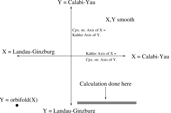
Figure 41: Area of Kähler sector of $X$ and $Y$ where we perform calculation.

The most general deformation of (10.1) consistent with this $({\mathbb{Z}}_{3})^{3}$ symmetry group is

$$W = a_{0}z_{0}z_{1}z_{2}z_{3}z_{4}+a_{1}z_{2}^{3}z_{4}^{9}+a_{2}z_{3}^{6}z_{4}^{6}+a_{3}z_{3}^{3}z_{4}^{12}+a_{4}z_{2}^{3}z_{3}^{3}z_{4}^{3}$$ (10.4)

$$+a_{5}z_{0}^{3}+a_{6}z_{1}^{3}+a_{7}z_{2}^{6}+a_{8}z_{3}^{9}+a_{9}z_{4}^{18}=0~{}.$$

One can show that $h^{2,1}(Y)=7$. The group of reparametrizations of (10.4) is indeed $({\mathbb{C}}^{*})^{5}$ as required which shows that we obtain 5 deformations of complex structure induced by deformations of (10.4). Note that for both $X$ and $Y$ we had 7 deformations of which only 5 will be analyzed via toric geometry. It is no coincidence that these numbers match — it follows from the monomial-divisor mirror map.

10.4 The Moduli Spaces

Let us now build the cones in $A_{n-1}(V)_{\mathbb{R}}$ to form the partial secondary fan. The method was outlined in subsection 9.8. Again, we shall only carry this out for the partially enlarged moduli space, although it is not much harder to do the fully enlarged case. We first build the $4\times 9$ matrix $A$ with columns $\alpha_{1},\ldots,\alpha_{9}$. From this we build the $9\times 5$ matrix $B$ whose columns span the kernel of $A$. The rows of $B$ give vectors in $A_{n-1}(V)_{\mathbb{R}}$. Note that a change of basis of the kernel of $A$ thus corresponds to a linear transformation on $A_{n-1}(V)_{\mathbb{R}}$. In order for us to translate the coordinates in $A_{n-1}(V)_{\mathbb{R}}$ into data concerning the coefficients $a_{i}$ in the complex structure of $Y$ we need to chose a specific basis in $A_{n-1}(V)_{\mathbb{R}}$.

We have already fixed $a_{0}=1$. We still have a $({\mathbb{C}}^{*})^{4}$ action on the other $a_{1},\ldots,a_{9}$ by which can fix 4 of these coefficients equal to one. Let us choose $a_{5}=a_{6}=a_{7}=a_{8}=1$ and denote the matrix that corresponds to this choice as $B_{1}$. Our 5 degrees of freedom are given by $\{a_{1},a_{2},a_{3},a_{4},a_{9}\}$. We want that a point with coordinates $(b_{1},b_{2},b_{3},b_{4},b_{5})$ in $A_{n-1}(V)_{\mathbb{R}}$ corresponds to $\{a_{1}=e^{2\pi i(c_{1}+ib_{1})},a_{2}=e^{2\pi i(c_{2}+ib_{2})},\ldots,a_{9}=e^{2\pi i(c_{5}+ib_{5})}\}$ for some value of the $B$-field $(c_{1},\ldots,c_{5})$. This means our matrix $B_{1}$ should be of the form

$$B_{1}=\left(\matrix{1&0&0&0&0\cr 0&1&0&0&0\cr 0&0&1&0&0\cr 0&0&0&1&0\cr B_{5,1}&B_{5,2}&B_{5,3}&B_{5,4}&B_{5,5}\cr B_{6,1}&B_{6,2}&B_{6,3}&B_{6,4}&B_{6,5}\cr B_{7,1}&B_{7,2}&B_{7,3}&B_{7,4}&B_{7,5}\cr B_{8,1}&B_{8,2}&B_{8,3}&B_{8,4}&B_{8,5}\cr 0&0&0&0&1\cr}\right).$$

$B_{1}$ is now completely determined by the condition that its columns span the kernel of $A$.

For the actual calculation below, we use a slightly different set of coordinates, choosing $\{a_{0},a_{1},a_{2},a_{3},a_{4}\}$ as the 5 degrees of freedom and setting $a_{5}=a_{6}=a_{7}=a_{8}=a_{9}=1$. (We do this to express (10.4) in the form: “Fermat + perturbation”, in order to more easily apply the calculational techniques of [10].) The new basis can be obtained from $B_{1}$ by using a ${\mathbb{C}}^{*}$ action $\lambda:z_{4}\rightarrow\lambda z_{4}$. We obtain the following matrix:

$$B=\left(\matrix{0&1&0&0&0\cr 0&0&1&0&0\cr 0&0&0&1&0\cr 0&0&0&0&1\cr\vphantom{\displaystyle\sum}-{\scriptstyle 1\over 3}&0&0&0&0\cr\vphantom{\displaystyle\sum}-{\scriptstyle 1\over 3}&0&0&0&0\cr\vphantom{\displaystyle\sum}-{\scriptstyle 1\over 6}&-{\scriptstyle 1\over 2}&0&0&-{\scriptstyle 1\over 2}\cr\vphantom{\displaystyle\sum}-{\scriptstyle 1\over 9}&0&-{\scriptstyle 2\over 3}&-{\scriptstyle 1\over 3}&-{\scriptstyle 1\over 3}\cr\vphantom{\displaystyle\sum}-{\scriptstyle 1\over 18}&-{\scriptstyle 1\over 2}&-{\scriptstyle 1\over 3}&-{\scriptstyle 2\over 3}&-{\scriptstyle 1\over 6}\cr}\right).$$

For each of the resolutions $\Delta_{1},\ldots,\Delta_{5}$ we can now construct the corresponding cone in $\Sigma^{\prime}$ following the method in subsection 9.8 using the $B$ matrix above. These five cones are shown schematically in figure 42 and the explicit coordinates in table 6.

Figure 42: The partial secondary fan.

Table 6: Generators for first cone.

 

 $$v_{1}$$  

 

   

 

   

 

   

 

   

 

Table 7: Generators for all cones.

   Resolution  Generators      $$\Delta_{1} v_{1} v_{2} v_{3} v_{4} v_{5} \Delta_{2} v_{1} v_{1}-v_{2}+v_{3}+v_{4} v_{3} v_{4} v_{5} \Delta_{3} v_{1} v_{2} v_{2}-v_{3}+v_{4} v_{4} v_{5} \Delta_{4} v_{1} v_{2} v_{3} v_{2}+v_{3}-v_{4}+v_{5} v_{5} \Delta_{5} v_{1} v_{2} v_{3} v_{2}+v_{3}-v_{4}+v_{5} v_{1} v_{2} v_{3}+(v_{2}+v_{3}-v_{4}+v_{5})-v_{5}$$  , , , ,      , , , ,      , , , ,      , , , ,      , , , ,  , ,  

Note that as expected the fan we generate, $\Sigma^{\prime}$, is not a complete fan and does not therefore correspond to a compact Kähler moduli space. This is a reflection of our working only with the partially enlarged moduli space — the geometrical models only fill out part of the full moduli space.

We now wish to translate this moduli space of Kähler forms into the equivalent structure in the moduli space of complex structures on $Y$. The way that we picked the basis in the $B$ matrix in this section tells us exactly how to proceed. For a point $(u_{0},u_{1},\ldots,u_{4})$ in $A_{n-1}(V)_{{\mathbb{R}}}$ we define

$$w_{k}=e^{2\pi i(c_{k}+iu_{k})}~{},$$ (10.5)

for any real $c_{k}$. This is then mapped to (10.4) by

$$a_{i} = w_{i}^{-1},\quad i=0,\ldots,4~{},$$ (10.6)

$$a_{i} = 1,\quad i=5,\ldots,9~{}.$$ (10.7)

This map explicitly tells us how to approach infinity in the complex structure moduli space of $Y$ to arrive at the putative mirror of a given large radius point in $X$. The five directions so generated are precisely those used in the calculation of section 7.6. As we showed in that section, ratios of correlation functions agree exactly in corresponding limits.

Although we will not discuss it in these lectures, we note for completeness that the fully enlarged Kähler moduli space of $X$ has 95 other regions in addition to these five geometric ones. One of these is a Landau-Ginzburg region, 27 are singular Calabi-Yau regions (strings propogating on Calabi-Yau’s with orbifold singularities) and 67 are regions which are “hybrids” of these others. As yet, no one has studied this hybrid models in any significant detail.

11 The Web of Connected Calabi-Yau Manifolds

In section 8, we have seen that type II string theory provides us with a mechanism for physically realizing topology changing transitions through conifold degenerations. This naturally raises two related questions:

1. Are all Calabi-Yau manifolds interconnected through a web of such transitions?

2. Are there other kinds of singularities, besides the ordinary double points discussed above, which might have qualitatively different physics and which might also have an important role in extending the Calabi-Yau web?

In this section we discuss some work presented in [34] which is relevant to these two questions. Related work can be found in [14, 45, 90] and references therein. The background we have developed in toric geometry plays a central role.

11.1 Extending the Mathematical Web of Calabi-Yau Manifolds

In an important series of papers [25, 26], it was argued some time ago that all Calabi-Yau manifolds realized as complete intersections in products of (ordinary) projective spaces are mathematically connected through conifold degenerations. As we mentioned above, although an intriguing prospect, it previously seemed that string theory did not avail itself of these topology changing transitions — as discussed, perturbative string theory is inconsistent at conifold points. The recent work described above shows that inclusion of non-perturbative effects cures the physical inconsistencies, at least in type II string theory, and hence the physical theory does allow such topology changing transitions to occur.

Since the time of [25, 26], the class of well studied Calabi-Yau manifolds has grown. Initially inspired by work of Gepner [53], the class of hypersurfaces in weighted projective four-dimensional spaces has received a significant amount of attention [68, 86, 27]. It was shown in [77, 80] that there are 7555 Calabi-Yau spaces of this sort. Inspired by mirror symmetry, another class of Calabi-Yau spaces (containing these 7555 hypersurfaces) that have been under detailed study are complete intersections in toric varieties [4, 113]. Understanding the structure of the moduli space of type II vacua requires that we determine if all of these Calabi-Yau spaces are interconnected through a web of topology changing transitions.

In the following we will describe a systematic procedure for finding transitions between Calabi-Yau manifolds realized as complete intersections in toric varieties. The method is elementary although at the present time there aren’t any general results on its range of applicability. Rather, the usefulness of this method becomes apparent by directly applying it to a subclass of the Calabi-Yau spaces realized in this manner. For instance, using the approach discussed below, all 7555 Calabi-Yau hypersurfaces in weighted projective four-dimensional space are mathematically connected to the web. We say mathematically because the transitions this procedure yields are not all of the conifold sort. Rather, there are Calabi-Yau spaces connected through more complicated singularities than the ordinary double points used in [67], as described in section 8. For example, some of these singularities are such that electrically and magnetically charged black hole states become simultaneously massless giving us an analog of the phenomenon discussed in [1]. Arguing for physical transitions through these theories requires more care than those involving conifold points. Whereas the term conifold transition refers to Calabi-Yau spaces linked through conifold degenerations, the term extremal transitions [88] refers to analogous links through any of the singularities at finite distance encountered on the discriminant locus. At present there is only a fully satisfying physical understanding of the conifold subclass of extremal transitions.

The procedure described below is relevant for Calabi-Yau spaces embedded in toric varieties and this was another motivation for the material in section 9.

To keep the discussion here concise, we shall focus on the case of hypersurfaces in weighted projective four-dimensional spaces, although we shall briefly mention some generalization at the end of this section. As discussed in [16] and reviewed in section 9, the data describing such Calabi-Yau manifolds is:

1. A lattice $N\simeq{\mathbb{Z}}^{4}$ and its real extension $N_{{\mathbb{R}}}=N\otimes_{{\mathbb{Z}}}{\mathbb{R}}$.

2. A lattice $M={\rm Hom}(N,{\mathbb{Z}})$ and its real extension $M_{\mathbb{R}}=M\otimes_{\mathbb{Z}}{\mathbb{R}}$.

3. A reflexive polyhedron $P\subset M_{\mathbb{R}}$.

4. The dual (or polar) polyhedron $P^{\circ}\subset N_{\mathbb{R}}$.

Now, given the above sort of toric data for two different families of Calabi-Yau spaces in two different weighted projective four-dimensional spaces, how might we perform a transition from one to the other? Well, given the polyhedra $(P,P^{\circ})$ for one Calabi-Yau and $(Q,Q^{\circ})$ for the other, one has the natural manipulations of set theory to relate them: namely, the operations of taking intersections and unions. Consider then, for instance, forming new toric data by taking the intersection

$$R={\rm convex~{}hull}\Big{(}(P\cap M)\cap(Q\cap M)\Big{)}~{}.$$

Further assume that $R$ (and its dual $R^{\circ}$) are reflexive polyhedra so that the singularities encountered are at finite distance in the moduli space [70]. How are the three Calabi-Yau spaces $X,Y,Z$ associated to $(P,P^{\circ})$, $(Q,Q^{\circ})$ and $(R,R^{\circ})$ respectively, related? As discussed in section 9, the toric data contained in the polyhedron in $M_{\mathbb{R}}$ is well known to describe the complex structure deformations of the associated Calabi-Yau realized via monomial deformations of its defining equation. Concretely, the lattice points in $P\cap M$ are in one-to-one correspondence with monomials in the defining equation of $X$, and similarly for $Y$ and $Z$. Thus, in going from $X$ to $Z$ we have specialized the complex structure by restricting ourselves to a subset of the monomial deformations. This is reminiscent of the example studied earlier, in which we specialized the complex structure of the quintic from its original $101$-dimensional moduli space to an $86$-dimensional subspace. This is not the end of the story. Clearly the dual $R^{\circ}$ contains $P^{\circ}$. As discussed earlier, the toric data contained in the polar polyhedron describes the Kähler structure deformations of the associated Calabi-Yau. Concretely, lattice points in $P^{\circ}\cap N$ correspond to toric divisors which are dual to elements in in $H^{2}(X,{\mathbb{Z}})$. Thus, in passing from $X$ to $Z$ we have also added toric divisors, i.e. we have performed a blow-up. This again is reminiscent of the example studied earlier: after specializing the complex structure we performed a small resolution. All of the discussion we have just had relating $X$ to $Z$ can be similarly applied to relate $Y$ to $Z$. Hence, by using the toric data associated to $X$ and to $Y$ to construct the toric data of $Z$, we have found that $Z$ provides a new Calabi-Yau that both $X$ and $Y$ are linked to in the web.

Of course, the key assumption in the above discussion is that $(R,R^{\circ})$ provides us with toric data for a Calabi-Yau, i.e. they are reflexive polyhedra. At present, there isn’t a general method for picking $(P,P^{\circ})$ and $(Q,Q^{\circ})$ such that this is necessarily the case. In fact, the toric data for a given Calabi-Yau is not unique but, for instance, depends on certain coordinate choices. Thus the reflexivity of $(R,R^{\circ})$ or lack thereof depends sensitively on the coordinate choices used in representing $(P,P^{\circ})$ and $(Q,Q^{\circ})$. Hence, a more appropriate question is whether there exists suitable representations of $(P,P^{\circ})$ and $(Q,Q^{\circ})$ such that $(R,R^{\circ})$ is reflexive. In [34], an exhaustive search was carried out in the following manner. The toric data $(P,P^{\circ})$ and $(Q,Q^{\circ})$, was arbitrarily chosen from the set of 7555 hypersurfaces. A variety of coordinate representations for each (related by $SL(5,{\mathbb{Z}})$ transformations and coordinate permutations) were considered and directly checked to see if $(R,R^{\circ})$ obtained from their intersection is reflexive. When such an $(R,R^{\circ})$ is reflexive, we learn that $X$ and $Y$ are (mathematically) connected through the Calabi-Yau $Z$. We note that, in general, $Z$ is not associated to a Calabi-Yau hypersurface in a weighted projective space — but rather a Calabi-Yau embedded in a more general toric variety.

In this manner, by direct computer search, it was checked that all 7555 hypersurfaces in weighted projective four-dimensional space are linked (and through the process described we have actually linked them up to numerous other Calabi-Yau spaces — the $Z$-type Calabi-Yau spaces above). The main physical question, then, is what is the nature of the singularities encountered when we specialize the complex structure in the manner dictated by the intersection of $P$ and $Q$. Analysis of the simplest examples shows that one often encounters singularities which are qualitatively different from the well understood case of several ordinary double points studied in [67], considered previously.

To illustrate this point, and the discussion of this section more generally, let us consider two explicit examples.

11.2 Two Examples

Example 1:

Let us take $X$ to be the family of quintic Calabi-Yau hypersurfaces in ${\mathbb{C}}P^{4}$ and $Y$ to be the family of Calabi-Yau hypersurfaces of degree 6 in $W{\mathbb{C}}P^{4}(1,1,1,1,2)$. The Hodge numbers of $X$ are $(h^{2,1}_{X},h^{1,1}_{X})=(101,1)$ and those of $Y$ are $(h^{2,1}_{Y},h^{1,1}_{Y})=(103,1)$. Following the procedure described above and using the discussion of chapter 9 $P^{\circ}\cap N$ is given by

$$\matrix{(1&0&0&0)~{},\cr(0&1&0&0)~{},\cr(0&0&1&0)~{},\cr(0&0&0&1)~{},\cr(-1&-1&-1&-1)~{},\cr}$$ (11.8)

and $Q^{\circ}\cap N$ by

$$\matrix{(1&0&0&0)~{},\cr(0&1&0&0)~{},\cr(0&0&1&0)~{},\cr(0&0&0&1)~{},\cr(-1&-1&-1&-2)~{},\cr}$$ (11.9)

From these polyhedra we find that the toric data for family $Z$, $R^{\circ}$, is the convex hull of

$$\matrix{(1&0&0&0)~{},\cr(0&1&0&0)~{},\cr(0&0&1&0)~{},\cr(0&0&0&1)~{},\cr(-1&-1&-1&-1)~{},\cr(-1&-1&-1&-2)~{}.\cr}$$ (11.10)

Note that for ease of presentation we are taking unions of data in $N$ space which is dual to taking intersections in $M$ space, discussed above. Consider first the transition from $Y$ to $Z$. One can show that the singular subfamily obtained by specializing the complex structure of $Y$, in the manner discussed above, consists of Calabi-Yau spaces which generically have 20 ordinary double points all lying on a single ${\mathbb{C}}P^{2}$ and hence obeying one non-trivial homology relation. This, therefore, is another example of the conifold transitions described in section 8. Thus, we can pass from $Y$ to $Z$ in the manner discussed and the Hodge numbers change to $(h^{2,1}_{Z},h^{1,1}_{Z})=(103-20+1,1+1)=(84,2)$. The relation between $X$ and $Z$, though, is more subtle. In specializing the complex structure of $X$ dictated by the toric manipulation, we find a singular family of Calabi-Yau spaces, each generically having one singular point. The local description of this singularity, however, is not an ordinary double point, but rather takes the form

$$x^{2}+y^{4}+z^{4}+w^{4}=0~{}.$$ (11.11)

This singularity is characterized by Milnor number $27$ which means that there are $27$ homologically independent $S^{3}$’s, simultaneously vanishing at the singular point. Thus, the singularity encountered is quite unlike the case of ordinary double points.

Using standard methods of singularity theory [50], one can show that the intersection matix of these $S^{3}$’s is non-trivial and has rank 20. Mathematically, it is straightforward to show that the transition from $X$ to $Z$ through such a degeneration causes the Hodge numbers to make the appropriate change.

Physically, in contrast to the previous cases, not only are $A$-type cycles shrinking down, but some dual $B$-type cycles are shrinking down as well. From this we see a phenomenon akin to that studied in [1]: we appear to have electrically and magnetically charged states simultaneously becoming massless. It is such degenerations that require more care in establishing the existence of physical transitions. This also raises the interesting question of whether the web of Calabi-Yau spaces requires such transitions for its connectivity, or if by following suitable paths conifold transitions would suffice.

Example 2:

We take $X$ to be the family of quintic Calabi-Yau hypersurfaces in ${\mathbb{C}}P^{4}$ and we take $Y$ to be the family of Calabi-Yau hypersurfaces of degree 8 in $W{\mathbb{C}}P^{4}(1,1,1,1,4)$. As in the previous example, the transition from $Y$ to $Z$ just involves ordinary double points, so the discussion of [67] suffices. However, in passing from $X$ to $Z$ we encounter another type of singularity, known as a triple point. Namely, the generic Calabi-Yau in the subfamily of $X$ obtained by specialization of the complex structure contains a single singular point whose local description is

$$x^{3}+y^{3}+z^{3}+w^{3}=0~{}.$$ (11.12)

The Milnor number for this singularity is equal to 16, and thus in this example we have 16 vanishing three-cycles (homological to $S^{3}$’s) simultaneously shrinking to one point. The intersection matrix in this case has rank 10 and we thus again are dealing with a physical situation with massless electrically and magnetically charged particles.

11.3 Remarks

For ease, in our discussion above, we have focused on hypersurfaces in weighted projective four-dimensional space (which naturally led to hypersurfaces in more general toric varieties). We can carry out the same program on codimension $d$ Calabi-Yau spaces. For these it is best to use the full reflexive Gorenstein cone associated with the Calabi-Yau, but basically the idea is the same. For instance, the union of the Gorenstein toric fan (in the N lattice) for $W{\mathbb{C}}P^{5}(3,3,2,2,1,1)$ $(5,7)$ and $W{\mathbb{C}}P^{5}(3,3,2,2,2,1)$ $(5,8)$ is Gorenstein with index 2. Hence, these codimension two Calabi-Yau spaces are linked through such transitions.

In this manner links have been established between numerous Calabi-Yau spaces of codimension two and between Calabi-Yau spaces of codimension three. Furthermore, as in each of these classes it is not hard to construct Calabi-Yau spaces with simple toric representations of various codimension (toric representations, of course, are not unique), we can link together the webs of different codimension as well. For instance, the quintic hypersurface, which is a member of the 7555 hypersurface web, is also linked to the web of complete intersections in products of ordinary projective spaces. Hence, all such Calabi-Yau spaces are so linked.

We therefore do not know the full answer to the two questions that motivated the discussion of this chapter, but some insight has been gained into each.

11.4 Summary

We can summarize the major developments described in these lectures by the following two figures. In part (a) figure 43, we see the abstract form of a connected component of the moduli space of an $N=2$, $c=9$ conformal field theory, and its geometrical interpretation in terms of the complexified Kähler cone and the complex structure moduli space of the associated Calabi-Yau manifold. This is the picture which was accepted for some time.

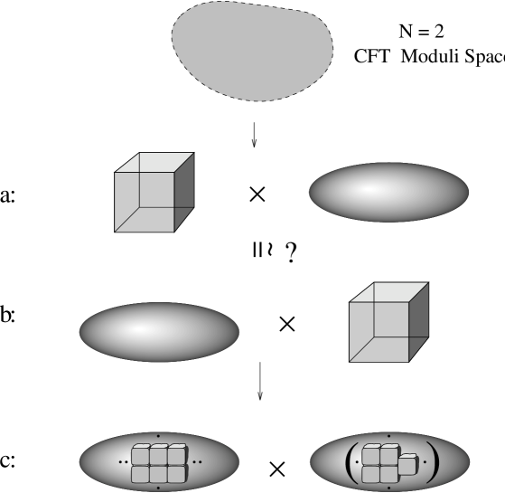
Figure 43: Models of the moduli space

When mirror symmetry was found, a new piece of this picture became apparent — given in part (b) of figure 43 — in which the abstract moduli space is also interpretable in terms of the complex structure and complexified Kähler structure of the mirror to the original Calabi-Yau. This, as we have discussed raised a puzzle since figures (a) and (b) in figure 43, which are supposed to be the geometrical incarnation of one and the same conformal field theory moduli space, are not isomorphic. The resolution, as we have discussed, is to enlarge the complexified Kähler moduli space in both figures (a) and (b) so that each now takes the form given in part (c) of figure 43. That is, the left hand side of part (a) is augmented to the left hand side of part (c), which is now isomorphic to the left hand side of part (b). Similarly for the right hand sides. We put parantheses around one part of the figure to note that in either geometrical interpretation ( (a) or (b) ) the phase structure has a natural physical interpretation on one side of the story — the Kähler sector. The physical interpretation of these phases, as we discussed at the end of section 5 is deepened by the work of [6] in which evidence is presented that each phase which appears to lack a direct geometric interpretation actually does have one so long as we analytically continue from an appropriate large radius Calabi-Yau region.

The non-perturbative results of this section build on this picture even further. In particular, we now see that the moduli space of non-perturbative string theory has a geometric interpretation that is far more rich than one would expect from perturbative considerations. It appears that all of these distinct connected components of conformal field theory moduli space join together into a single component of type II string theory moduli space. This is heuristically sketched in figure 44, which is the picture that has finally emerged.

Figure 44: The structure of the moduli space as has emerged from these lectures.

12 Conclusions

In these lectures, we have sought to give the reader some understanding of the emerging field of quantum geometry. The basic philosophy we have followed is to allow the physics of $N=2$ space-time supersymmetric string theory to be our guide towards the correct geometrical framework for describing string theory. We have seen that this analysis has naturally led us to some unexpected consequences. Foremost amongst these is the realization that one underlying string model may, in fact, have two distinct non-linear sigma model realizations — that is, with two distinct target spaces. When the explicit isomorphism between these two realizations involves flipping the sign of one of the $U(1)$ charges in the $N=2$ superconformal algebra, we call the two target spaces mirror manifolds. From the viewpoint of classical geometry, these two manifolds are distinct objects; for instance, they are topologically distinct. From the viewpoint of quantum geometry, as we have discussed, they are identical. This is a prime example of how classical and quantum geometry differ.

This distinction between classical and quantum geometry is dramatically augmented by the realization that topology change — an operation which by fundamental definition in classical geometry is discontinuous — can be perfectly continuous and smooth in the quantum geometry of string theory. We have seen this in the context of mild topology changing flop transitions which occur even at the level of classical perturbative string theory, and, strikingly, through the drastic topology changing conifold transitions. These, as we have seen, require non-perturbative string effects in an essential way.

We began these lectures by emphasizing that string duality does not respect the decomposition of perturbative/non-perturbative effects — in fact, that is the source of its tremendous power. In the case at hand, for instance, string duality allows certain conifold transitions in type II string theory to be mapped to heterotic transitions on $K3\times T^{2}$ as shown by [76] and as reviewed by Aspinwall in this volume. Remarkably, in the heterotic language, the transitions are perturbative in nature.

Clearly, string theory is really forcing us to broaden our understanding of the way in which geometrical data determines observable physics. One can’t help feeling that we are only catching glimpses of the proverbial iceberg’s tip — understanding the mathematics and physics underlying string duality is certain to expose it further and deeply affect our conceptions of this remarkable unified theory.

References

- [1] P. Argyres and M. Douglas, Nucl. Phys. B448 (1995) 93.
- [2] P. S. Aspinwall, Commun. Math. Phys. 128 (1990) 593.
- [3] P. S. Aspinwall, B. R. Greene and D. R. Morrison, Internat. Math. Res. Notices (1993) 319.
- [4] P. S. Aspinwall, B. R. Greene and D. R. Morrison, Nucl. Phys. B416 (1994) 414.
- [5] P. S. Aspinwall and B. R. Greene, Nucl. Phys. B437 (1995) 205.
- [6] P. S. Aspinwall, B. R. Greene and D. R. Morrison, Nucl. Phys. B420 (1994) 184.
- [7] P. S. Aspinwall, “The Moduli Space of Superconformal Field Theories” in Proceedings of Trieste Summer School, Trieste 1994.
- [8] P. S. Aspinwall and D. R. Morrison, “String Theory on K3 Surfaces” in Essays in Mirror Manifolds II, International Press 1995.
- [9] P. S. Aspinwall and D. R. Morrison, Commun. Math. Phys. 151 (1993) 245.
- [10] P. S. Aspinwall, C. A. Lütken, and G. G. Ross, Phys. Lett. B241 (1990) 373.
- [11] P. S. Aspinwall, B. R. Greene and D. R. Morrison, “Space-Time Topology Change: The Physics of Calabi-Yau Moduli Space” in Proceedings of Strings ‘93 Conference, Berkeley 1993.
- [12] P. S. Aspinwall and C. A. Lütken, Nucl. Phys. B355 (1991) 482.
- [13] M. Audin, “The Topology of Torus Actions on Symplectic Manifolds”, Progress in Math., vol. 93, Birkhäuser, 1991.
- [14] A. C. Avram, P. Candelas, D. Jancic and M. Mandelberg, Nucl. Phys. B465 (1996) 458.
- [15] T. Banks, L. Dixon, D. Friedan and E. Martinec, Nucl. Phys. B299 (1988) 613.
- [16] V. Batyrev, J. Alg. Geom. 3 (1994) 493.
- [17] V. Batyrev and L. A. Borisov, “On Calabi-Yau Complete Intersections in Toric Varieties”, alg-geom/9412017.
- [18] V. Batyrev and D. van Straten, “Generalized Hypergeometric Functions and Rational Curves on Calabi-Yau Complete Intersections in Toric Varieties”, Essen preprint, 1993.
- [19] K. Becker, M. Becker and A. Strominger, Nucl.Phys. B456 (1995) 130.
- [20] P. Berglund and S. Katz, “Mirror Symmetry Constructions: A Review” in Essays in Mirror Manifolds II, International Press 1995.
- [21] M. Bershadsky, V. Sadov and C. Vafa, Nucl. Phys. B463 (1996) 398.
- [22] L.J. Billera, P. Filliman, and B. Sturmfels, Adv. Math. 83 (1990) 155.
- [23] L. A. Borisov, “Towards the Mirror Symmetry for Calabi-Yau Complete Intersections in Gorenstein Toric Fano Varieties”, alg-geom/9310001.
- [24] P. Candelas, Nucl. Phys. B298 (1988) 458.
- [25] P. Candelas, P. S. Green and T. Hübsch, Phys. Rev. Lett. 62 (1989) 1956;
- [26] P. Candelas, P. S. Green, and T. Hübsch, Nucl. Phys. B330 (1990) 49.
- [27] P. Candelas, M. Lynker and R. Schimmrigk, Nucl. Phys. B341 (1990) 383.
- [28] P. Candelas and X. de la Ossa, Nucl. Phys. B355 (1991) 455.
- [29] P. Candelas, X. de la Ossa, A. Font, S. Katz and D.R. Morrison, “Mirror Symmetry for Two Parameter Models: I”, CERN preprint CERN-TH.6884/93.
- [30] P. Candelas, X. C. de la Ossa, P. S. Green, and L. Parkes, Phys. Lett. B258 (1991) 118.
- [31] P. Candelas, X. C. de la Ossa, P. S. Green, and L. Parkes, Nucl. Phys. B359 (1991) 21.
- [32] A. Ceresole, R. D’ Auria, S. Ferrara and A. Van Proeyen, Nucl. Phys. B444 (1995) 92.
- [33] T. Chiang and B. Greene, “Phases of mirror symmetry”, hep-th/9509049.
- [34] T. Chiang, B. Greene, M. Gross and Y. Kanter, “Black Hole Condensation and the Web of Calabi-Yau Manifolds” in Proceedings of Trieste Duality Conference, Trieste 1995.
- [35] H. Clemens, Adv. Math. 47 (1983) 107.
- [36] S. Coleman, QFT lectures (unpublished).
- [37] D.A. Cox, “The Homogeneous Coordinate Ring of a Toric Variety”, Amherst preprint, 1992.
- [38] M. Dine, N. Seiberg, X.-G. Wen, and E. Witten, Nucl. Phys. B278 (1987) 769.
- [39] M. Dine, N. Seiberg, X.-G. Wen, and E. Witten, Nucl. Phys. B289 (1987) 319.
- [40] J. Distler, “Notes on -models” in Proceedings of Trieste Spring School, World Scientific 1992.
- [41] J. Distler and B. Greene, Nucl. Phys. B309 (1988) 295.
- [42] L. Dixon, “Some World Sheet Properties of Superstring Compactifications, on Orbifolds and Otherwise” in Superstrings, Unified Theories and Cosmology 1987, G. Furlan et al., eds., World Scientific 1988.
- [43] L. Dixon, J. Harvey, C. Vafa and E. Witten, Nucl. Phys. B261 (1985) 678.
- [44] L. Dixon, J. Harvey, C. Vafa and E. Witten, Nucl. Phys. B274 (1986) 285.
- [45] M. R. Douglas, S. Katz and C. Vafa, “Small Instantons, Del Pezzo Surfaces and Type I Prime Theory”, hep-th/9609071.
- [46] C. J. Efthimiou and B. R. Greene, Geometrical Concepts in Physics (in preparation).
- [47] D. Friedan, A. Kent, S. Shenker and E. Witten, unpublished.
- [48] A. Font, Nucl. Phys. B 391 (1993) 358.
- [49] W. Fulton, Introduction to Toric Varieties, Ann. Math. Studies, vol. 131, Princeton University Press 1993.
- [50] A. M. Gabrielov, Functional Anal. Appl. 7(3) 18.
- [51] I. M. Gel’fand, M. M. Kapranov and A. V. Zelevinsky, Func. Anal. Appl. 28 (1989) 12.
- [52] I. M. Gel’fand, M. M. Kapranov and A. V. Zelevinsky, Adv. Math. 84 (1990) 255.
- [53] D. Gepner, Phys. Lett. B199 (1987) 380.
- [54] D. Gepner, Nucl. Phys. B296 (1987) 380.
- [55] D. Gepner, in Proceedings of Trieste Spring School, World Scientific 1989.
- [56] D. Gepner and Z. Qiu, Nucl. Phys. B285 [FS19](1987) 423.
- [57] P. Ginsparg, “Applied Conformal Field Theory”, in Proceedings of Les Houches summer school, North Holland 1989.
- [58] A. Giveon, M. Porrati and E. Rabinovici, Phys. Rep. 244 (1994) 77.
- [59] M. Green and J. Schwarz, Phys. Lett. B149 (1984) 117.
- [60] P. Green and T. Hübsch, Commun. Math. Physics 101 (1985) 341.
- [61] P. Green and T. Hübsch, Commun. Math. Phys. 113 (1987) 505.
- [62] Essays on Mirror Manifolds II, B.R. Greene and S-T. Yau, ed., International Press 1996.
- [63] B. R. Greene, C. Vafa and N. Warner, Nucl. Phys. B324 (1989) 371.
- [64] B. R. Greene and R. Plesser, Nucl. Phys. B338 (1990) 15.
- [65] B. R. Greene and R. Plesser, “An Introduction to Mirror Manifolds” in Essays in Mirror Manifolds, International Press 1991.
- [66] B. R. Greene, in Essays in Mirror Manifolds II, International Press 1996.
- [67] B. R. Greene, D. R. Morrison and A. Strominger, Nucl. Phys. B451 (1995) 109.
- [68] B. R. Greene, C. Vafa, and N. P. Warner, Nucl. Phys. B324 (1989) 371.
- [69] P. Griffiths and J. Harris, Principles of Algebraic Geometry, John Wiley & Sons 1994.
- [70] Y. Hayakawa, “Degeneration of Calabi-Yau Manifold with Weil-Petersson Metric”, alg-geom/9507016.
- [71] T. Hübsch, Calabi-Yau Manifolds, A Bestiary for Physicists, World Scientific 1992.
- [72] G. Horowitz and A. Strominger, Nucl. Phys. B360 (1991) 197.
- [73] S. Hosono, A. Klemm and S. Theisen, “Lectures on Mirror Symmetry” in Integrable Models and Strings, A. Alekseev, A. Hietamäki, K. Huitu, A. Morozov and A. Niemi, eds.
- [74] S. Hosono, A. Klemm, S. Theisen and S.-T. Yau, “Mirror Symmetry, Mirror Map and Applications to Calabi-Yau Hypersurfaces”, Harvard preprint HUTMP-93/0801.
- [75] C. M. Hull and P. K. Townsend Nucl.Phys. B438 (1995) 109.
- [76] S. Kachru and C. Vafa, Nucl. Phys. B450 (1995) 69.
- [77] A. Klemm and R. Schimmrigk, Nucl. Phys B411 (1994) 559.
- [78] A. Klemm and S. Theisen, Nucl. Phys. B 389 (1993) 153.
- [79] J. Kollár, Nagoya Math. J. 113 (1989) 15.
- [80] M. Kreuzer and H. Skarke, Nucl. Phys. B388 (1992) 113.
- [81] S. Lefschetz, “L’ Analysis Situs et la Géométrie Algébraique,” Gautier-Villars, Paris, 1924; reprinted in Selected Papers, Chelsea, New York, 1971, p. 283-439, for an extremely clear discussion oriented for physicists see [25, 26].
- [82] W. Lerche, C. Vafa and N. Warner, Nucl. Phys. B324 (1989) 427.
- [83] A. Libgober and J. Teitelbaum, Int. Math. Res. Notices (1993) 15.
- [84] J. Lykken, “Introduction to Supersymmetry” in this volume.
- [85] E. Martinec, Phys. Lett. 217 (1989) 431.
- [86] E. Martinec, “Criticality, Catastrophes and Compactifications” in V.G. Knizhnik Memorial Volume, L. Brink, et al., eds., World Scientific 1990.
- [87] D.R. Morrison, in Essays on Mirror Manifolds, S.-T. Yau, ed., International Press 1991.
- [88] D. R. Morrison, “Through the Looking Glass”, Lecture at CIRM Conference, Trento (June, 1994), to appear.
- [89] D. R. Morrison and R. Plesser, “Towards Mirror Symmetry as Duality for Two-Dimensional Abelian Gauge Theories” in STRINGS 95: Future Perspectives, Los Angeles 1995.
- [90] D. R. Morrison and N. Seiberg, “Extremal Transitions and Five-Dimensional Supersymmetric Field Theories”, hep-th/9609070.
- [91] T. Oda, Convex Bodies and Algebraic Geometry, Springer-Verlag, 1988.
- [92] T. Oda and H.S. Park, Tôhoku Math. J. 43 (1991) 375.
- [93] H. Ooguri, “Lectures on Perturbative String Theories” in this volume.
- [94] H. Ooguri, Y. Oz and Z. Yin, Nucl. Phys. B477 (1996) 407.
- [95] J. Polchinski, “Lectures on D-Branes” in this volume.
- [96] J. Polchinski, Phys. Rev. Lett. 75 (1995) 4724.
- [97] J. Polchinski and E. Witten, Nucl. Phys. B460 (1996) 525.
- [98] M. Reid, in Journées de géometrie algébrique d’ Angers (A. Beauville, ed.), Sijthoff & Noordhoff, 1980, p. 273.
- [99] S.-S. Roan, Int. J. Math. 1 (1990) 211.
- [100] J. Schwarz, Banff Summer Inst., 1988:55-123 (QCD161:B23:1988).
- [101] S. Shenker, “Another Length in String Theory?”, hep-th/9509132.
- [102] N. Seiberg and E. Witten, Nucl. Phys. B426 19.
- [103] A. Sen, Nucl. Phys. B278 (1987) 423.
- [104] A. Strominger and E. Witten, Commun. Math. Phys. 101 (1985) 341.
- [105] A. Strominger, Phys. Rev. Lett. 55 (1985) 2547.
- [106] A. Strominger, Nucl. Phys. B451 (1995) 96.
- [107] A. Strominger, S.-T. Yau and E. Zaslow, Nucl. Phys. B479 (1996) 243.
- [108] C. Vafa, Mod. Phys. Lett. A4 (1989) 1169.
- [109] N. P. Warner, “Lectures on Superconformal Theories and Singularity Theory” in Proceedings of Trieste Spring School, World Scientific 1989.
- [110] P. West, Introduction to Supersymmetry and Supergravity, 2nd edition, World Scientific 1990.
- [111] E. Witten, Nucl. Phys. B188 (1982) 513.
- [112] E. Witten, Int. J. Mod. Phys. A9 (1994) 4783.
- [113] E. Witten, Nucl. Phys. B403 (1993) 159.
- [114] E. Witten, Nucl. Phys. B443 (1995) 85.
- [115] E. Witten, “Some Comments on String Dynamics” in STRINGS 95: Future Perspectives in String Theory, Los Angeles 1995.
- [116] E. Witten, Nucl. Phys. B460 (1996) 335.
- [117] S.-T. Yau, ed., Essays on Mirror Manifolds I, International Press 1996.
- [118] A. B. Zamolodchikov and V. A. Fateev, Sov. Phys. JETP 63 (1986) 91.
- [119] B. Zumino, Phys. Lett. B87 (1979) 203.