LBNL-039423, UCB-PTH-97/09

hep-th/9702154

Branes and Mirror Symmetry in $N=2$ Supersymmetric Gauge Theories in Three Dimensions
Jan de Boer, Kentaro Hori, Yaron Oz and Zheng Yin

Department of Physics, University of California at Berkeley
366 Le Conte Hall, Berkeley, CA 94720-7300, U.S.A.
and
Theoretical Physics Group, Mail Stop 50A–5101
Ernest Orlando Lawrence Berkeley National Laboratory, Berkeley, CA 94720, U.S.A.

We use brane configurations and $SL(2,{\bf Z})$ symmetry of the type IIB string to construct mirror $N=2$ supersymmetric gauge theories in three dimensions. The mirror map exchanges Higgs and Coulomb branches, Fayet-Iliopoulos and mass parameters and $U(1)_{R}$ symmetries. Some quantities that are determined at the quantum level in one theory are determined at the classical level of the mirror. One such example is the complex structure of the Coulomb branch of one theory, which is determined quantum mechanically. It is mapped to the complex structure of the Higgs branch of the mirror theory, which is determined classically. We study the generation of $N=2$ superpotentials by open D-string instantons in the brane configurations.

1 Introduction

Recently brane configurations that preserve $\frac{1}{8}$ of space-time supersymmetry of type II string theory have been used to study $N=1$ duality in four dimensions [2]. Similar configurations can be used, upon T-dualizing one of the coordinates, to study $N=2$ supersymmetric gauge theories in three dimensions. In [3, 4, 5, 6, 7] a mirror symmetry between $N=4$ gauge theories in three dimensions has been studied. In this paper we will study a similar mirror symmetry between $N=2$ gauge theories in three dimensions.

The $N=2$ supersymmetry algebra in three dimensions is only invariant under one $U(1)_{R}$ symmetry. Therefore, a priori there is no notion of mirror symmetry which, as in $N=2$ in two dimensions and $N=4$ in three dimensions, exchanges two commuting R-symmetries acting differently on the supercharges. However, there are theories having extra global symmetries commuting with the supercharges. If we combine the $U(1)_{R}$ symmetry with these global symmetries, we may be able to have two $U(1)_{R}$ symmetries which act differently on the moduli space of vacua, and we can introduce a notion of mirror symmetry under which these two $U(1)_{R}$’s are exchanged. One purpose of this paper is to realize this by the use of the brane configuration of [2] and application of type IIB $SL(2,{\bf Z})$ duality following [6].

The $N=2$ gauge theories can be constructed as the dimensional reduction of $N=1$ gauge theories in four dimensions. The bosonic part of the $N=2$ vector multiplet contains the three dimensional gauge field $A_{\mu}$ and a real scalar $\varphi$ which corresponds to the $A_{4}$ component of the four dimensional gauge field. The action contains the term ${\rm Tr}[A_{\mu},A_{\nu}]^{2}$ and the term ${\rm Tr}[A_{\mu},\varphi]^{2}$. Thus, the low energy effective theory is described by the abelian theory in which $\varphi$ and $A_{\mu}$ belong to a common Cartan sub-algebra of the gauge group. In three dimensions the photon $A_{\mu}$ is dual to a scalar field $\sigma$. The vacuum expectation values of the scalars $\varphi$ and $\sigma$ parameterize the Coulomb branch of the theory. The Coulomb branch has real dimension $2r$ where $r$ is the rank of the gauge group. Due to $N=2$ supersymmetry it is a Kähler manifold of complex dimension $r$. Note that this differs from $N=1$ theories in four dimensions where there are no scalars in the vector multiplet and therefore there is no Coulomb branch. Matter fields are in the $N=2$ chiral multiplet. The scalar fields in the multiplet parameterize the Higgs branch, which is determined by the D- and F-term equations. By $N=2$ supersymmetry, it is also a Kähler manifold.

In addition to the R-symmetry, the system possesses flavor symmetries depending on the matter content. Also, there are global symmetries corresponding to the shifts of $\sigma$ by a constant. In non-abelian gauge theories, some of these symmetries can be broken by instanton configuration, but some combinations remain exact (although they might be spontaneously broken [8]). Taking suitable combinations of $U(1)_{R}$ and other global symmetries, we can get two $U(1)$ R-symmetries with respect to which we can divide the moduli space into two parts. The two parts will still be called the Coulomb and the Higgs branch, and in a pair of mirror symmetric gauge theories it is these two parts that are exchanged. The mass parameters that exist already in four dimensions are complex and charged with respect to a $U(1)_{R}$ symmetry, while the FI parameters are real and do not carry a $U(1)_{R}$ charge. Therefore, unlike the $N=4$ case we should not expect a naive exchange of these parameters. Indeed, as we will see there are many more parameters so that a precise map between the parameters of the mirror theories is possible.

In $N=2$ supersymmetric non-abelian gauge theory in three dimensions, a superpotential may be generated both for the Higgs and the Coulomb branches by instantons which in three dimensions are BPS monopoles. We will study this from the viewpoint of string theory by considering open D-string instantons.

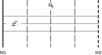
Figure 1: Brane configuration for an $N=2$ $U(N_{c})$ gauge theory with $N_{f}$ flavors in three dimensions.

We will mainly consider two brane setups in type IIB string theory for studying the $N=2$ theories. The first configuration is depicted in figure 1. It consists of one NS 5-brane whose worldvolume has the coordinates $(x^{0}x^{1}x^{2}x^{3}x^{4}x^{5})$, one NS^′ 5-brane whose worldvolume has the coordinates $(x^{0}x^{1}x^{2}x^{3}x^{8}x^{9})$, $N_{c}$ D3 branes stretching between them in the $x^{6}$ direction with worldvolume $(x^{0}x^{1}x^{2}x^{6})$ and $N_{f}$ D5 branes with worldvolume $(x^{0}x^{1}x^{2}x^{7}x^{8}x^{9})$. This configuration preserves $\frac{1}{8}$ of the $32$ space-time supersymmetries. We consider the supersymmetric gauge theory obtained as the long distance limit of the worldvolume dynamics of the D3 brane. This is an $N=2$ supersymmetric gauge theory with $U(N_{c})$ gauge group and $N_{f}$ pairs of chiral multiplets in the (anti-)fundamental of the gauge group.

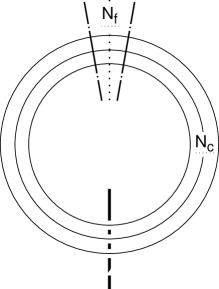
Figure 2: Brane configuration for an $N=2$ $U(N_{c})$ gauge theory with $N_{f}$ flavors and three adjoints in three dimensions.

The second configuration is depicted in figure 2. It consists of an NS 5-brane whose worldvolume has the coordinates $(x^{0}x^{1}x^{2}x^{3}x^{8}x^{9})$, $N_{c}$ D3 branes stretching in the $x^{6}$ direction with worldvolume $(x^{0}x^{1}x^{2}x^{6})$, and $N_{f}$ D5 branes with worldvolume at coordinates $(x^{0}x^{1}x^{2}x^{7}x^{8}x^{9})$. The $x^{6}$ coordinate is compactified on a circle. This configuration also preserves $\frac{1}{8}$ of the $32$ space-time supersymmetries. We consider the supersymmetric gauge theory on the worldvolume of the D3 brane with coordinates $(x^{0}x^{1}x^{2})$. This is an $N=2$ supersymmetric gauge theory with $U(N_{c})$ gauge group, $N_{f}$ pairs of chiral multiplets in the (anti-)fundamental representation of the gauge group and three chiral multiplets in the adjoint representation. The two extra pairs of massless chiral multiplets in the adjoint representation arise from the compactification of the $x^{6}$ coordinate on a circle. The field content falls into representations of $N=4$ supersymmetry. However half of this supersymmetry is broken by the superpotential.

2 Mirror Symmetry in Abelian $N=2$ Theories

2.1 A-Model

Consider the brane configuration of figure 1 with one D3 brane ($N_{c}=1$ case). In the long distance limit, the worldvolume of the D3 brane describes an $N=2$ $U(1)$ gauge theory with $N_{f}$ pairs of chiral multiplets of charges $+1,-1$. The brane configuration is invariant under rotations in the $(x^{4},x^{5})$ and $(x^{8},x^{9})$ directions and these correspond to the global symmetries $U(1)_{4,5}$ and $U(1)_{8,9}$ of the three dimensional gauge theory.

The light fields on the D3 brane worldvolume are:

$\bullet$ An open string ending on the D3 brane yields an $N=8$ $U(1)$ vector multiplet. Only one of the seven scalars of the multiplet remains after imposing the boundary condition at the NS and NS^′ ends. Therefore only an $N=2$ $U(1)$ vector multiplet remains. The value $x^{3}({\rm D3})$ (the $x^{3}$-coordinate of the D3 brane) corresponds to the scalar field $\varphi$ in the vector multiplet. The vector $A_{0,1,2}$ is dual to the scalar field $\sigma$. These scalars are singlets under both $U(1)$’s. The fermions carry charge $\pm 1$ under both $U(1)_{4,5}$ and $U(1)_{8,9}$ .

$\bullet$ Open strings ending on the D3 brane and the $i$-th D5 brane yield chiral multiplets $Q_{i}$ and $\widetilde{Q}_{i}$ of opposite charges $+1$ and $-1$. The scalar components are singlet under $U(1)_{4,5}$ but carry charge $+1$ of $U(1)_{8,9}$. The fermions carry charge $-1$ of $U(1)_{4,5}$ and are singlets under $U(1)_{8,9}$.

The positions of NS, NS^′ and the D5 brane correspond to parameters of the three dimensional field theory.

$\bullet$ The difference $x^{7}({\rm NS})-x^{7}({\rm NS}^{\prime})$ of the positions of the NS and ${\rm NS}^{\prime}$ 5-branes in the $x^{7}$ direction is the Fayet-Iliopoulos parameter $\zeta^{\bf r}$ of the $U(1)$ gauge theory. It is invariant under the global $U(1)$ symmetries.

$\bullet$ The position $x^{3}({\rm D}5_{i})$ of the $i$-th D5 brane in the $x^{3}$ direction is the real mass parameter $m^{\bf r}_{i}$ of the $i$-th quark. A real mass can be considered as a scalar component of $N=2$ vector multiplet of the flavor symmetry group $U(N_{f})$. It is invariant under the global $U(1)$ symmetries. Note that the center of mass $\sum_{i=1}^{N_{f}}m_{i}^{\bf r}$ can be absorbed by a shift of $\varphi$ and is not a physical parameter.

$\bullet$ The position $x^{4,5}({\rm D}5_{i})$ of the $i$-th D5 brane in the $x^{4},x^{5}$ is the complex mass parameter $m_{i}$ of the $i$-th quark which is present already in the four dimensional $N=1$ theory. Since it transforms in the vector representation of $SO(2)_{4,5}$ it carries charge $2$ of $U(1)_{4,5}$ and is singlet under $U(1)_{8,9}$.

To summarize, we list the fields and parameters of the gauge theory with their transformation properties under the global symmetry group $U(1)_{4,5}\times U(1)_{8,9}$. Note that both $U(1)$’s can be considered as R-symmetry groups acting on a chiral superfield $\Phi(\theta)$ as $\Phi(\theta)\rightarrow{\rm e}^{Q_{\Phi}i\alpha}\Phi({\rm e}^{-i\alpha}\theta)$.

$$\begin{array}[]{cccl}&U(1)_{4,5}&U(1)_{8,9}&\\ \varphi,\sigma&0&0&\\ Q_{i}&0&1&\,\,i=1,\ldots,N_{f}\\ \widetilde{Q}_{i}&0&1&\,\,i=1,\ldots,N_{f}\\ \zeta^{\bf r}&0&0&\\ m_{i}^{\bf r}&0&0&\,\,i=1,\ldots,N_{f}\\ m_{i}&2&0&\,\,i=1,\ldots,N_{f}\end{array}$$ (2.1)

The theory has the tree level superpotential

$$W=\sum_{i=1}^{N_{f}}m_{i}\widetilde{Q}_{i}Q_{i}.$$ (2.2)

Note that $U(1)_{45}$ is broken explicitly by the complex mass parameter.

As we mentioned in the introduction there is another global $U(1)$ symmetry acting only on $\sigma$:

$$\sigma\longmapsto\sigma\,+\,\,{\rm constant}.$$ (2.3)

The flavor symmetry group $SU(N_{f})\times SU(N_{f})$ is broken to $U(1)^{N_{f}-1}\times U(1)^{N_{f}-1}$ by the diagonal mass matrix. Some of these symmetries are invisible in the brane configuration. Notice that the (independent) flavor symmetry group is not $U(N_{f})\times U(N_{f})$, because the central $U(1)^{2}$ are already present in the theory as the $U(1)$ gauge symmetry and the axial part of $U(1)_{4,5}\times U(1)_{8,9}$.

In the abelian gauge theory in three dimensions, there are neither perturbative nor non-perturbative effects that break any of these $2N_{f}+1$ $U(1)$ global symmetries. These are exact symmetries of the quantum theory, although spontaneous symmetry breaking is possible [8].

2.2 B-Model

Let us now perform an $SL(2,{\bf Z})$ transformation on the above configuration. Before the application of it, we move the NS 5-brane to the right in the $x^{6}$ direction, crossing one D5 brane. After an $SL(2,{\bf Z})$ transformation we end up with the configuration of figure 3.

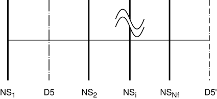
Figure 3: $SL(2,Z)$ of the brane configuration of $N=2$ $U(1)$ gauge theory with $N_{f}$ flavours.

The light fields on the D3 brane worldvolume are :

$\bullet$ An open string ending on the D3 brane stretched between the ${\rm NS}_{i}$ and ${\rm NS}_{i+1}$ 5-branes yields an $N=4$ $U(1)$ vector multiplet, consisting of an $N=2$ $U(1)$ vector multiplet $W_{i}$ and a neutral chiral multiplet $\Phi_{i}$. The value $x^{7}(D3)$ and vector field $A_{0,1,2}$ corresponds to the scalars $\varphi_{i}$, $\sigma_{i}$ of $W_{i}$ while the values $x^{8,9}(D3)$ combine into the complex scalar of $\Phi_{i}$.

$\bullet$ An open string ending on the D3 brane stretched between the ${\rm NS}_{N_{f}}$ and ${\rm D}^{\prime}$ 5-branes yields an $N=2$ neutral chiral multiplet $M$. The values $x^{8,9}(D3)$ correspond to the complex scalar component of $M$.

$\bullet$ Open strings ending on the D5 brane and the D3 brane which is stretched between the ${\rm NS}_{1}$ and ${\rm NS}_{2}$ 5-branes yield an $N=4$ hypermultiplet $Q$, $\widetilde{Q}$ charged under the first $U(1)_{1}$ of the $N=4$ vector multiplet $(W_{1},\Phi_{1})$. The hypermultiplet is coupled in an $N=4$ supersymmetric way, i.e. with a nonzero superpotential involving $Q,\widetilde{Q},\Phi_{1}$ from the $N=2$ point of view.

$\bullet$ Open strings ending on the D3 branes in the $i$-th and $i+1$-th interval yield an $N=4$ hypermultiplet charged as $(+1,-1)$ under the $i$-th and $i+1$-th gauge group $U(1)_{i}\times U(1)_{i+1}$. For $i=1,\ldots,N_{f}-2$, we denote it by $b_{i,i+1}$, $b_{i+1,i}$ and for $i=N_{f}-1$, we denote it by $\widetilde{q}$, $q$.

The $N=2$ chiral multiplet $M$ (“meson”) can be interpreted as a remnant of an $N=4$ vector multiplet of the $U(1)$ flavor group rotating $q$, $\widetilde{q}$, and there is a term $M\widetilde{q}q$ in the superpotential. Thus we have an $N=4$ supersymmetric $U(1)^{N_{f}-1}$ gauge theory broken to $N=2$ via coupling to a neutral $N=2$ chiral multiplet by superpotential. This is illustrated in figure 4.

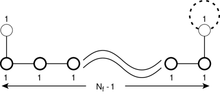
Figure 4: Quiver like diagram for the B-model. The dashed circle correspond to the meson.

The positions of NS D and D^′ 5-branes are parameters of the field theory.

$\bullet$ The difference $x^{3,4,5}({\rm NS}_{i})-x^{3,4,5}({\rm NS}_{i+1})$ of positions of the $i$-th and $i+1$-th NS 5-branes in the $x^{3}x^{4}x^{5}$ is the Fayet-Iliopoulos parameter $\zeta^{3,4,5}_{i}$ of the $N=4$ vector multiplet $(W_{i},\Phi_{i})$. We denote $\zeta^{3}_{i}=\zeta^{\bf r}_{i}$ and $\zeta^{4,5}_{i}=\zeta_{i}$.

$\bullet$ If the difference $x^{4,5}({\rm NS}_{N_{f}})-x^{4,5}({\rm D}^{\prime}5)$ is non-zero, there cannot be a D3 brane stretched in the interval ${\rm NS}_{N_{f}}$-${\rm D}^{\prime}5$. Since the meson $M$ created by the D3 brane is a remnant of the $N=4$ flavor $U(1)$ vector multiplet, the difference is an analog of the Fayet-Iliopoulos parameter $\zeta_{M}$ which enters in the superpotential as $\zeta_{M}M$.

$\bullet$ The difference $x^{7}({\rm D}5)-x^{7}({\rm D}^{\prime}5)$ forbids a Higgs branch corresponding to a D3 brane stretched between the D and ${\rm D}^{\prime}$ 5-branes, and it can be interpreted as the real bare mass $m_{q}^{\bf r}$ of the quark $q,\widetilde{q}$. Note that other mass parameters can be absorbed by the shift of $\varphi_{i}$, $\Phi_{i}$ and $M$.

To summarize, we list the fields and the parameters of the gauge theory. Notice that the number of parameters is $3N_{f}$, the same as in the A-model. As in the previous case, we can read the R-charges of the two $U(1)$ symmetry groups from the brane configuration.

$$\begin{array}[]{cccl}&U(1)_{4,5}&U(1)_{8,9}&\\ \varphi_{i},\sigma_{i}&0&0&\,\,i=1,\ldots,N_{f}-1\\ \Phi_{i}&0&2&\,\,i=1,\ldots,N_{f}-1\\ M&0&2&\\ Q,\widetilde{Q}&1&0&\\ b_{i,i+1},b_{i+1,i}&1&0&\,\,i=1,\ldots,N_{f}-2\\ q,\widetilde{q}&1&0&\\ \zeta^{\bf r}_{i},\zeta_{i}&0\oplus 2&0\oplus 0&\,\,i=1,\ldots,N_{f}-1\\ \zeta_{M}&2&0&\\ m_{q}^{\bf r}&0&0&\end{array}$$ (2.4)

The theory possesses the tree level superpotential

$$W=W_{N=4}+M\widetilde{q}q-\zeta_{M}M,$$ (2.5)

where $W_{N=4}$ is the superpotential of the $N=4$ sector

$$W_{N=4}=\sum_{i=1}^{N_{f}-1}\Phi_{i}\Bigl{(}b_{i,i-1}b_{i-1,i}-b_{i,i+1}b_{i+1,i}-\zeta_{i}\Bigr{)}$$ (2.6)

in which we denoted $Q,\widetilde{Q}=b_{1,0},b_{0,1}$ and $q,\widetilde{q}=b_{N_{f},N_{f}-1},b_{N_{f}-1,N_{f}}$. In addition to $U(1)_{4,5}\times U(1)_{8,9}$, we have global symmetry group $U(1)^{N_{f}}$ acting as $(q,\widetilde{q})\mapsto({\rm e}^{i\beta_{0}}q,{\rm e}^{-i\beta_{0}}\widetilde{q})$; $\sigma_{i}\mapsto\sigma_{i}+\beta_{i}$; ($i=1,\ldots,N_{f}-1$). These $N_{f}+2$ global $U(1)$ symmetries are exact in the quantum theory, although they might be spontaneously broken. Note that we seem to be missing global $U(1)^{N_{f}-1}$ compared with the A-model. This is a symmetry that arises quantum mechanically and is not manifest in the classical Lagrangian. A similar phenomenon has been found and explained in [3] for $N=4$ supersymmetric theories.

2.3 Verification Of The Mirror Symmetry

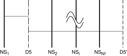
Figure 5: The Higgs branch of the B-model.

There are two phases in brane configurations corresponding to both of the A and B models. In the configuration of A-model, one phase corresponds to the D3 brane ending on NS and NS^′ 5-branes and moving in the $x^{3}$ direction (Coulomb branch), while in the second phase it is broken into $N_{f}+1$ pieces by letting the D3 branes end on D5 branes and the pieces move in the $(x^{7}),x^{8},x^{9}$ directions (Higgs branch). In the configuration of B-model, in the first phase the $N_{f}+1$ pieces of D3 branes end on NS and NS or NS and D^′ 5-branes and move in $(x^{7}),x^{8},x^{9}$ directions (Coulomb branch), while in the second phase the D3 brane is broken into two at the D5 brane and one of them moves in the $x^{3}$ direction ending on D and D^′ 5-branes as in figure 5 (Higgs branch). In the next subsection we will see that this distinction of branches is natural from the viewpoint of the action of the $U(1)$ R-symmetries.

In $N=2$ supersymmetric field theory in three dimensions, there are no loop corrections to the F-term by the perturbative non-renormalization theorem [8]. Moreover, in abelian gauge theory, we expect no non-perturbative effect, and thus there is no dynamical generation of a superpotential in these models. However, there are loop corrections to the D-term, and thus we can at most compare the complex structure of the moduli spaces of vacua. The complex structure of Higgs branch is determined at the classical level, and is expected to be unchanged by quantum corrections. However, the Coulomb branch is obtained after a duality transformation, and the global structure may be changed in the dual variables. Nevertheless, we expect that, like in the $N=4$ case [10], the global and complex structure can be determined by looking at the behavior at infinity of the moduli space, and that a one-loop analysis is sufficient to determine them. It turns out that the one loop Coulomb branch does have a natural complex structure, and as in the case of Higgs branch it will not be further corrected. Thus, we compare the complex structure of one loop corrected Coulomb branch of the A-model and the classical Higgs branch of the B-model.

2.3.1 ${\cal M}_{C}(\mbox{A-Model})={\cal M}_{H}(\mbox{B-Model})$

A Coulomb branch of the A-model is possible only when the FI parameter $\zeta^{\bf r}$ vanishes, while a Higgs branch of the B-model is possible only when the real bare mass $m_{q}^{\bf r}$ is zero. Therefore, we can identify $\zeta^{\bf r}=m_{q}^{\bf r}$.

We first consider the one loop metric of the Coulomb branch of the A-model. Now it is useful to consider the model — $N=2$ supersymmetric QED with $N_{f}$ electrons — as “embedded” in the corresponding $N=4$ model whose mass 3-vector $\vec{m}_{i}$ is given by $(m_{i}^{\bf r},m_{i})$. The only difference in the one loop computation of the Coulomb branch metric is that the $N=4$ vector multiplet contains a neutral chiral multiplet $\Phi$ which provides the center of complex bare mass of the electrons. Thus, the one loop metric of the $N=2$ Coulomb branch is given by the one loop metric of the $N=4$ Coulomb branch restricted to the hyperplane $\Phi=m_{\rm c}:=\sum_{i}m_{i}/N_{f}$. In [4], the one loop metric on the $N=4$ Coulomb branch has been computed. In the limit where the bare coupling $1/e^{2}\rightarrow 0$, it is the ALE space of $A_{N_{f}-1}$ type whose $\zeta$ parameters are given by $\vec{m}_{i}-\vec{m}_{i-1}$ ($i=1,\ldots,N_{f}$; $\vec{m}_{0}:=\vec{m}_{N_{f}-1}$). Thus, the Coulomb branch of the A-model is given by

$$\Bigl{\{}\,\,\Phi=m_{\rm c}\,\,\Bigr{\}}\subset\mbox{ALE}_{A_{N_{f}-1}}\bigl{(}\,\vec{m}_{i}-\vec{m}_{i-1}\,\bigr{)}.$$ (2.7)

The limit $1/e^{2}\rightarrow 0$ was also taken while studying the mirror symmetry in $N=4$ theories and corresponds to taking the IR limit.

It is also useful to note that the $N=4$ sector of the B-model is the one first considered in [3] as the mirror of $N=4$ QED with $N_{f}$ electrons. Since the model is obtained by coupling it to the $N=2$ meson sector via the superpotential (2.6), the only difference in the Higgs branch is that there is an extra constraint $\partial W/\partial M=0$. The $N=4$ Higgs branch is again the ALE space whose $\zeta$ parameters are given by $\vec{\zeta}_{i}=\zeta_{i}^{3,4,5}$ ($i=0,1,\ldots,N_{f}-1$; $\vec{\zeta}_{0}:=-\sum_{i}\vec{\zeta}_{i}$). Thus, the $N=2$ Higgs branch is given by

$$\Bigl{\{}\,\,\widetilde{q}q=\zeta_{M}\,\,\Bigr{\}}\subset\mbox{ALE}_{A_{N_{f}-1}}\bigl{(}\,\,\vec{\zeta}_{i}\,\,\bigr{)}.$$ (2.8)

That these two have the same complex structure under a certain relation of $\vec{m}_{i}$ and $\vec{\zeta}_{i}$, $\zeta_{M}$ can be seen by looking at the one loop computation given in Section 4 of [4]. In fact, they are the same submanifold of the same hyper-Kähler manifold whose defining equation is holomorphic with respect to one distinguished complex structure. To illustrate this, let us consider the case in which all the bare masses are the same ($m_{i}=m_{\rm c}$) in the A-model and all the FI parameters are vanishing ($\vec{\zeta}_{i}=0$) in the B-model. In this case, both ALE spaces coincide with the orbifold ${\bf C}^{2}/{\bf Z}_{N_{f}}$. Let $(z_{1},z_{2})$ be the coordinates of ${\bf C}^{2}$ on which ${\bf Z}_{N_{f}}$ acts by $(z_{1},z_{2})\mapsto({\rm e}^{2\pi il/N_{f}}z_{1},{\rm e}^{-2\pi il/N_{f}}z_{2})$. In the A-model, $\varphi$, $\sigma$, $\Phi$ are expressed in terms of $z_{1},z_{2}$ by $\varphi=|z_{1}|^{2}-|z_{2}|^{2}$, $\sigma=2{\rm arg}(z_{1})$, and $\Phi=z_{1}z_{2}$. By introducing the ${\bf Z}_{N_{f}}$ invariant coordinates, $x=z_{1}^{N_{f}}$, $y=z_{2}^{N_{f}}$ the Coulomb branch of the A-model is described by

$$xy=m_{\rm c}^{N_{f}}\,.$$ (2.9)

The Higgs branch of the B-model is determined in this case by the equations $|b_{i,i+1}|=|\widetilde{Q}|=|\widetilde{q}|$, $|b_{i+1,i}|=|Q|=|q|$, $b_{i,i+1}b_{i+1,i}=\widetilde{Q}Q=\widetilde{q}q$, and $\widetilde{q}q=\zeta_{M}$ modulo gauge transformations. Using gauge invariant coordinates $x=Qq\prod_{i=1}^{N_{f}-2}b_{i+1,i}$, $y=\widetilde{Q}\widetilde{q}\prod_{i=1}^{N_{f}-2}b_{i,i+1}$, it is expressed as

$$xy=\zeta_{M}^{N_{f}},$$ (2.10)

which is the same as (2.9) if we identify $m_{\rm c}=\zeta_{M}$.

2.3.2 ${\cal M}_{H}(\mbox{A-Model})={\cal M}_{C}(\mbox{B-Model})$

When we turn off all the mass parameters of the A-model and set the vev of the scalars in the vector multiplet to zero, we get a Higgs branch of maximal dimension in which $Q_{i}$ and $\widetilde{Q}_{i}$ are turned on. The classical D-term equation is given by

$$\sum_{i=1}^{N_{f}}|Q_{i}|^{2}-\sum_{i=1}^{N_{f}}|\widetilde{Q}_{i}|^{2}=\zeta^{\bf r}.$$ (2.11)

The Higgs branch is obtained as the $U(1)$ quotient of the set of solutions. This is the standard Kähler quotient of $({\bf C}\oplus{\bf C}^{\vee})^{\oplus N_{f}}$ by the $U(1)$ action. As a complex manifold, it is obtained as the quotient of $({\bf C}\oplus{\bf C}^{\vee})^{\oplus N_{f}}$ by the ${\bf C}^{\times}$ action, in which we throw away some “bad orbits” depending on the value of $\zeta^{\bf r}$. (A good explanation can be found in [11].) For $\zeta^{\bf r}\neq 0$, it is isomorphic to the total space of the direct sum of $N_{f}$ tautological bundles ${\cal O}(-1)^{\oplus N_{f}}$ over ${\bf C}{\bf P}^{N_{f}-1}$. For $\zeta^{\bf r}=0$, it is a singular space which is described by the quadratic relations $x_{i,k}x_{j,l}=x_{i,l}x_{j,k}$ where $x_{i,j}$ are the gauge invariant coordinates $x_{i,j}=Q_{i}\widetilde{Q}_{j}$.

For the B-model, when we turn off all the FI parameters and set the vev of $Q,\widetilde{Q},b_{i,i\pm 1},q,\widetilde{q}$ to zero, we obtain a Coulomb branch parameterized by $\varphi_{i},\sigma_{i},\Phi_{i},M$. Recall that the $N=4$ sector of the model is the model considered in [3] as a mirror of $N=4$ QED with $N_{f}$ electrons. Note that the meson $M$ provides the complex part of the mass $\vec{m}=(m_{q}^{\bf r},M)$ of the field $q,\widetilde{q}$. As computed in [4], the one loop corrected Coulomb branch of the $N=4$ model is the same as the classical Higgs branch of its mirror, $N=4$ QED with $N_{f}$ electrons, with its FI parameter given by $\vec{m}$. It is the set of $U(1)$ orbits of $(Q_{i},\widetilde{Q}_{i})$ satisfying

$$\sum_{i=1}^{N_{f}}|Q_{i}|^{2}-\sum_{i=1}^{N_{f}}|\widetilde{Q}_{i}|^{2}=m_{q}^{\bf r},$$ (2.12)

$$\sum_{i=1}^{N_{f}}\widetilde{Q}_{i}Q_{i}=M.$$ (2.13)

In the $N=2$ Coulomb branch $M$ is free to vary. This means that the second equation does not restrict the vev of $\widetilde{Q}_{i},Q_{i}$, and the Coulomb branch of the B-model is the same as the Higgs branch of the A-model, provided $\zeta^{\bf r}=m_{q}^{\bf r}$.

2.3.3 The Action of $U(1)$ R-Symmetry Groups

Recall that we have two $U(1)$ R-symmetries $U(1)_{4,5}$ and $U(1)_{8,9}$ coming from the invariance of the brane configuration. In this subsection, we shall see that these two $U(1)$’s, modified by combination with other global symmetries, act on Coulomb or Higgs branches, one group on one branch, the other on the other, and that these actions are interchanged under mirror symmetry.

In the A-model, we define $U(1)_{H}=U(1)_{8,9}$ and $U(1)_{C}$ as the diagonal subgroup of the product of $U(1)_{4,5}$ and the global $U(1)$ acting as shifts of $\sigma$. $U(1)_{C}$ acts on the coordinates and parameters of the Coulomb branch as $\sigma\mapsto\sigma+2\alpha$, $m_{i}\mapsto{\rm e}^{2i\alpha}m_{i}$, and $U(1)_{H}$ acts on the Higgs branch as $Q_{i},\widetilde{Q}_{i}\mapsto{\rm e}^{i\alpha}Q_{i},{\rm e}^{i\alpha}\widetilde{Q}_{i}$.

In the B-model, we define $U(1)_{H}=U(1)_{4,5}$ and $U(1)_{C}$ as the diagonal of the product of $U(1)_{8,9}$ and the global $U(1)$ acting as shifts of $\sigma_{i}$. $U(1)_{C}$ acts on the Coulomb branch as $\sigma_{i}\mapsto\sigma_{i}+2\alpha$, $(\Phi_{i},M)\mapsto({\rm e}^{2i\alpha}\Phi_{i},{\rm e}^{2i\alpha}M)$, while $U(1)_{H}$ acts on the Higgs branch as multiplication by ${\rm e}^{i\alpha}$ on $Q,\widetilde{Q},b_{i,i\pm 1},q,\widetilde{q}$ and multiplication by ${\rm e}^{2i\alpha}$ on $\zeta_{i},\zeta_{M}$.

To see that $U(1)_{C}$ and $U(1)_{H}$ of the A-model is mapped to $U(1)_{H}$ and $U(1)_{C}$ of the B-model, we recall the transformation mapping two $SU(2)$ doublet ${\bf 2}\times{\bf 2}$ to ${\bf 1}\oplus{\bf 3}$, which was used in the comparison of the Coulomb and Higgs branches of the $N=4$ mirror theories[4].

Let $(z_{1},\overline{z_{2}})$ be the coordinates of the $SU(2)$ doublets. In terms of the quaternion coordinate ${\bf q}=z_{1}+z_{2}j$, the $SU(2)$ action is the left multiplication by unit quaternions $Sp(1)\subset{\bf H}^{\times}$. We define $\sigma$ and $\vec{\varphi}=(\varphi^{1},\varphi^{2},\varphi^{3})$ by ${\bf q}=a{\rm e}^{i\sigma/2}$; $\overline{a}=-a$, and ${\bf q}i\overline{\bf q}=\varphi^{1}i+\varphi^{2}j+\varphi^{3}k$. Under an $SU(2)$ rotation, $\vec{\varphi}$ transforms as a vector ${\bf 3}$. With respect to the $U(1)$ subgroup $\{{\rm e}^{i\alpha}\}\subset Sp(1)$, $z_{1},z_{2}$ transform as ${\rm e}^{i\alpha}z_{1},{\rm e}^{i\alpha}z_{2}$, while $\sigma$, $\varphi^{1}=|z_{1}|^{2}-|z_{2}|^{2}$, and $\Phi:=\varphi^{2}+i\varphi^{3}=-2iz_{1}z_{2}$ transform as $\sigma\mapsto\sigma+2\alpha$, $\varphi^{1}\mapsto\varphi^{1}$ and $\Phi\mapsto{\rm e}^{2i\alpha}\Phi$.

We now observe that these transformations are indeed mapped into each other under the identification of the Coulomb branch of the A-model with the Higgs branch of the B-model, and vice versa.

3 Mirror Symmetry in Non-Abelian $N=2$ Theories

3.1 A-Model

Consider the brane configuration of figure 1 with $N_{c}$ D3 branes. In the long distance limit, the worldvolume of the D3 brane describes an $N=2$ $U(N_{c})$ gauge theory with $N_{f}$ pairs of chiral multiplets. As discussed in the previous section the brane configuration is invariant under rotation in the $(x^{4},x^{5})$ and $(x^{8},x^{9})$ directions and these correspond to global symmetries $U(1)_{4,5}$ and $U(1)_{8,9}$ of the three dimensional gauge theory.

As in the previous section we read from the brane configuration the fields and parameters of the gauge theory on the worldvolume of the D3 brane, and their transformation properties under the global symmetry group $U(1)_{4,5}\times U(1)_{8,9}$. This is summarized in the following.

$$\begin{array}[]{cccl}&U(1)_{4,5}&U(1)_{8,9}&\\ \varphi_{a},\sigma_{a}&0&0&\,\,a=1,\ldots,N_{c}\\ Q_{i}&0&1&\,\,i=1,\ldots,N_{f}\\ \widetilde{Q}_{i}&0&1&\,\,i=1,\ldots,N_{f}\\ \zeta^{\bf r}&0&0&\\ m_{i}^{\bf r}&0&0&\,\,i=1,\ldots,N_{f}\\ m_{i}&2&0&\,\,i=1,\ldots,N_{f}\end{array}$$ (3.1)

3.2 B-Model

Let us now perform an $SL(2,{\bf Z})$ transformation on the above configuration. Before the application of it, we move the NS 5-brane to the right in the $x^{6}$ direction, crossing $N_{c}$ D5 branes. We end up with the configuration of figure 6.

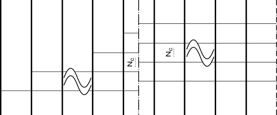
Figure 6: Brane configuration of the B-model.

The gauge group of the B-model is $U(N_{c})^{N_{f}-N_{c}}\prod_{i=1}^{N_{c}-1}U(i)$. For $N_{c}=1$ it reduces to the abelian duality of the previous section with gauge group $U(1)^{N_{f}-1}$.

Again we summarize the fields and parameters of the gauge theory on the worldvolume of the D3 brane, and their transformation properties under the global symmetry groups.

$$\begin{array}[]{cccl}&U(1)_{4,5}&U(1)_{8,9}&\\ \varphi_{i},\sigma_{i}&0&0&\,\,i=1,\ldots,N_{f}-1\\ \Phi_{i}&0&2&\,\,i=1,\ldots,N_{f}-1\\ M_{\alpha}&0&2&\,\,\alpha=1,\ldots,N_{c}\\ Q,\widetilde{Q}&1&0&\\ b_{i,i+1},b_{i+1,i}&1&0&\,\,i=1,\ldots,N_{f}-1\\ q_{\alpha},\widetilde{q}_{\alpha}&1&0&\,\,\alpha=1,\ldots,N_{c}\\ \zeta^{\bf r}_{i},\zeta_{i}&0\oplus 2&0\oplus 0&\,\,i=1,\ldots,N_{f}-1\\ \zeta_{M}&2&0&\\ m_{q}^{\bf r}&0&0&\end{array}$$ (3.2)

We follow the notations of the abelian case. The only difference is that now the fields carry also gauge indices of the corresponding gauge group which we abbreviated.

The $N=2$ meson $M$ couples to $q$, $\widetilde{q}$ by the term $\sum M_{\alpha}\widetilde{q}_{\alpha}q_{\alpha}$ in the superpotential. The B-model is an $N=4$ supersymmetric $U(N_{c})^{N_{f}-N_{c}}\prod_{i=1}^{N_{c}-1}U(i)$ gauge theory broken to $N=2$ by coupling to the $N=2$ sector via the superpotential, as in figure 7.

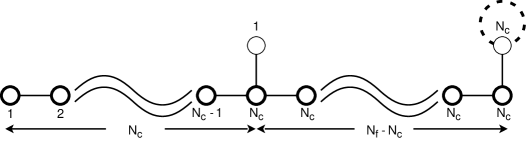
Figure 7: Quiver like diagram for the B-model.

As in the Abelian case we expect that the mirror map exchanges an appropriately defined Higgs and Coulomb branches. However, since in the non-Abelian theories we expect in general that superpotentials will be generated, the analysis of the previous section has to be modified. The full details of these modifications remain to be uncovered.

The $SL(2,Z)$ transformation suggests that the mirror map exchanges the FI and mass parameters of the A-model with the mass and FI parameters of the B-model

$$\zeta^{\bf r}=m_{q}^{\bf r},~{}~{}~{}~{}~{}m_{i}^{\bf r}-m_{i-1}^{\bf r}=\zeta_{i}^{\bf r},~{}~{}~{}~{}~{}i=1,...,N_{f}-1,$$ (3.3)

$$m_{c}=\zeta_{M},~{}~{}~{}~{}~{}m_{i}-m_{i-1}=\zeta_{i},~{}~{}~{}~{}~{}i=1,...,N_{f}-1,$$ (3.4)

where $m_{c}$ is the average of the complex mass parameters of the A-model.

4 Breaking $N=4$ by a superpotential

Mirror symmetry in three-dimensional $N=4$ gauge theories have been studied in [4, 7] based on quiver diagrams. In this section we study mirror $N=2$ gauge theories which are obtained from these $N=4$ by breaking half of the supersymmetry due to a vanishing superpotential.

4.1 A-Model

Consider the brane configuration in figure 2, with one NS 5-brane with coordinates $(x^{0}x^{1}x^{2}x^{3}x^{8}x^{9})$, $N_{f}$ Dirichlet 5-branes with coordinates $(x^{0}x^{1}x^{2}x^{3}x^{4}x^{5})$ and $N_{c}$ Dirichlet 3-branes with coordinates $(x^{0}x^{1}x^{2}x^{3})$. The coordinate $x^{3}$ is compactified on a circle. In the long distance limit, worldvolume theory of the D3 branes is that of $N=2$ supersymmetric theory with $U(N_{c})$ gauge group, $N_{f}$ pairs of chiral multiplets in the fundamental and the dual representations, and three massless chiral multiplets in the adjoint representation. Two extra adjoint chiral multiplets arise from the compactification of the coordinate $x^{3}$ on a circle. They will be denoted by $A,\widetilde{A}$. The $N=4$ supersymmetry is broken to $N=2$ since the superpotential vanishes. In order to see that the Yukawa coupling in the $N=4$ superpotential vanishes we list, as before, the fields, parameters and charges.

$$\begin{array}[]{cccl}&U(1)_{4,5}&U(1)_{8,9}&\\ \varphi,\sigma&0&0&\\ \Phi&0&2&\\ Q_{i},\widetilde{Q}_{i}&0&1&\,\,i=1,\ldots,N_{f}\\ A,\widetilde{A}&1&0&\\ m_{i}^{\bf r}&0&0&\,\,i=1,\ldots,N_{f}\\ m_{i}&2&0&\,\,i=1,\ldots,N_{f}\end{array}$$ (4.1)

Indeed the Yukawa coupling term $\widetilde{Q}\Phi Q$ does not carry the correct $U(1)$ charges and therefore is absent in the superpotential, thus breaking the $N=4$ supersymmetry to $N=2$. Since we have only one NS 5-brane, the FI parameters associated with the $U(1)$ factor in the gauge group vanishes. Note also that there are really only $N_{f}-1$ mass parameters, since one linear combination can be shifted by shifting $\varphi,\Phi$. The mass of the adjoint chiral multiplets is zero by construction.

4.2 B-Model

Performing an $SL(2,Z)$ on the configuration of figure 2 we get the configuration of figure 8.

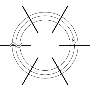
Figure 8: Brane configuration of the B-model obtained by $SL(2,Z)$ transformation of figure 2.

The list of the fields, parameters and charges reads now

$$\begin{array}[]{cccl}&U(1)_{4,5}&U(1)_{8,9}&\\ \varphi_{i},\sigma_{i}&0&0&\,\,i=1,\ldots,N_{f}\\ \Phi_{i}&0&2&\,\,i=1,\ldots,N_{f}\\ Q,\widetilde{Q}&0&1&\\ b_{i,i+1},b_{i+1,i}&1&0&\,\,i=1,\ldots,N_{f}\\ \zeta^{\bf r}_{i},\zeta_{i}&0\oplus 2&0\oplus 0&\,\,i=1,\ldots,N_{f}-1\\ \end{array}$$ (4.2)

where by $b_{N_{f},N_{f}+1}$ we mean $b_{N_{f},1}$. There are no mass parameters in the B-model since they can all be set to zero by shifting $\varphi_{i},\Phi_{i}$. Note also that there are only $N_{f}-1$ FI parameters since the sum of them vanishes $\sum_{i=1}^{N_{f}}\zeta^{\bf r}_{i}=\sum_{i=1}^{N_{f}}\zeta_{i}=0$. This corresponds to the fact that the mass of the adjoint chiral multiplets in the A-model is zero. The B-model has a tree level superpotential containing terms $b\Phi b$ and terms $Q\tilde{Q}bb$. In addition, there will in general be nonperturbative corrections to the superpotential. The precise form of these corrections is not known, and this obstructs a more detailed check of the mirror symmetry.

According to the $SL(2,Z)$ duality, the mirror map between the mass parameters of the A-model and the FI parameters of the B-model takes the form

$$m_{i}-m_{i-1}=\zeta_{i},~{}~{}~{}~{}~{}m_{i}^{\bf r}-m_{i-1}^{\bf r}=\zeta^{\bf r}_{i}~{}~{}~{}~{}~{}~{}~{}~{}~{}~{}i=1,...,N_{f}-1.$$ (4.3)

The above construction of mirror pairs generalizes in a straightforward way to all the mirror quiver diagrams of $N=4$ gauge theories that were discussed in [7].

5 Comments on $N=2$ Theories

5.1 Duality in Three Dimensions

In [2] a duality between $U(N_{c})$ and $U(N_{f}-N_{c})$ $N=1$ gauge theories in four dimensions has been studied. Upon T-duality in $x^{3}$, the same brane configurations can be used to study a similar duality in three dimensions. As an example, consider the brane configuration in figure 1 with one D3 brane and two D5 branes. It describes in the coordinates $(x^{0}x^{1}x^{2})$ $N=2$ $U(1)$ gauge theory with two pairs of chiral multiplets in the fundamental representation. Moving the NS 5-brane through the D5 branes using [6] and around the NS^′ 5-brane we get the configuration of figure 9, which describes a $U(1)$ gauge theory with two pairs of chiral multiplets in the fundamental and the dual representations $(q^{i},\tilde{q}_{\tilde{i}})$ , a meson $M_{i}^{\tilde{i}}$ and a superpotential $W=M_{i}^{\tilde{i}}q^{i}\tilde{q}_{\tilde{i}}$.

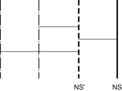
Figure 9: Brane configuration for an $N=2$ $U(1)$ gauge theory with two flavours, a meson and a superpotential.

The complex dimension of the Higgs branch of the theory we ended with is four while that of the original theory is three. The $U(1)$ gauge theories in three dimensions do not have monopoles and therefore there are no instanton corrections. Also we do not expect any strong dynamics that will generate a superpotential [12]. It is easy to see that a non perturbative generation of a superpotential is also forbidden by the $U(1)$ symmetries (3.1). Therefore, the classical counting of the dimensions of the Higgs branches is valid quantum mechanically. This suggests that the duality between $N=1$ $U(N_{c})$ and $U(N_{f}-N_{c})$ gauge theories in four dimensions [2] is not valid in three dimensions.

5.2 Superpotentials and Open D-String Instantons

It has been argued that nonperturbative dynamics of supersymmetric gauge theories in three dimensions is controlled by instantons [12]. In this section we will study instantons from string theory viewpoint and analyze their contribution to the superpotential. In three dimensions the instanton carries a magnetic charge. The magnetic charge is mediated by the scalar dual to the photon $\sigma$ [13]. The instantons from the string theory viewpoint are the D-strings that end on the D3 branes[6, 7]. The boundary of a D-string is the worldline of a magnetic monopole in the D3 brane [14]. To break half of the supersymmetry, it must be holomorphically embedded [15], which in this case means being flat and orthogonally intersecting other branes. To qualify as an instanton configuration for the effective three dimensional theory, the D-string worldvolume must be Euclidean and compact. Therefore it must be bounded on all sides.

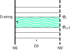
Figure 10: Open D-string instanton generation of a superpotential.

One such instanton is illustrated in figure 10, a D-string stretched (shaded region) between parallel pairs of D3 and NS 5-branes. They are the $SL(2,Z)$ dual of the open string instantons of [16, 15]. Here we consider a generic point in the Coulomb branch of the moduli space, so the $U(N_{c})$ gauge group on the D3 worldvolume is broken to its maximal Abelian subgroup. The $\varphi$’s are the VEV’s of the expectation values of the scalars in the vector multiplets. They also parameterize the positions of the D3 branes in the $x^{3}$ direction. We use the convention that $\varphi_{i}>\varphi_{i+1}$. A monopole of charge $(n_{1},n_{2}-n_{1},n_{3}-n_{2}\dots,n_{N_{c}-1}-n_{N_{c}-2},-n_{N_{c}-1})$ with respect to the unbroken $U(1)$’s can be thought of as a multi-monopole solution made up of $n_{i}$ fundamental monopoles of the i-th type. The latter have charges $1$ and $-1$ with respect to the i-th and (i+1)-th $U(1)$ respectively and 0 for the rest [17]. This has a straightforward interpretation in string theory. The i-th fundamental open D-string instanton is represented by the shaded area in figure 10. More general instanton configuration are just combination of this type.

The instanton contributions to the path integral take the form of $K^{\prime}e^{-S_{0}-i\sigma}$ [13], where $K^{\prime}$ is a factor that includes the one loop determinant and $S_{0}$ is the classical action for the instanton background $S_{0}\sim-\frac{\varphi}{e^{2}}$. $\sigma$ is the dual to the photon of the unbroken $U(1)$. It emerges from field theory after summing the instantons in the dilute instanton gas approximation [13, 8]. It is also expected by holomorphy arguments. All these have a counterpart in string theory language.

Naturally, instanton corrections in string theory come in the form of

$$Ke^{-S_{\rm{D-string}}}$$ (5.1)

where K is a factor that includes the one-loop determinant of the massive fields on the D-string worldsheet, and $S_{\rm{D-string}}$ is the D-string worldsheet action. This action contains two pieces:

$$S_{0}=S_{\rm Nambu-Goto}+i\int_{\rm boundary}\tilde{A}\cdot dX,$$ (5.2)

The Nambu-Goto action simply yields the area of the Euclidean D-string divided by the tension of the D-string [7]. Thus

$$S_{Nambu-Goto}={\mbox{area}}\times{\rm{tension}}=\frac{[(\varphi_{i}-\varphi_{i+1})\alpha^{\prime}]\times[g_{\rm st}/{e^{2}}]}{g_{st}\alpha^{\prime}}=\frac{\varphi_{i}-\varphi_{i+1}}{e^{2}}\mskip 6.0mu,$$ (5.3)

where we used the relation between the three dimensional gauge coupling $e$, the string coupling $g_{\rm st}$ and the distance $r$ between the NS 5-branes in the $x^{6}$ direction: $\frac{1}{e^{2}}=\frac{r}{g_{\rm st}}$.

In addition, there is the contribution from the boundary of the D-string. It couples to the electric and magnetic gauge potential on the D5 and D3 branes with coupling constants $g$ of the respective theories. The former is not dynamical but the latter is important. Denote the magnetic and electric gauge potentials and field strengths by tilded and untilded symbols respectively, then

$$\epsilon_{ijk}F_{ij}=g_{\rm st}\tilde{F}_{k6}=g_{\rm st}(\partial_{k}\tilde{A}_{6}-\partial_{6}\tilde{A}_{k}),$$ (5.4)

where $i,j,k$ take value among $0,1,2$. Applying $SL(2,Z)$ to the discussion in [6], one deduces that when a D3 brane ends on two NS 5-branes, the magnetic gauge field vanishes in the effective three dimensional theory but $\tilde{A}_{6}$ survives. Equation (5.4) now reads

$$\epsilon_{ijk}F_{ij}=g_{\rm st}\partial_{k}\tilde{A}_{6}.$$ (5.5)

Thus $g_{\rm st}\tilde{A}_{6}=e^{2}\sigma$ is the dual of the photon. The contribution of the second term in (5.4) is now

$$\int_{boundary}\tilde{A}\cdot dX={\sigma_{i}-\sigma_{i+1}}$$ (5.6)

Therefore the correction from such an instanton is proportional to

$$e^{-((\varphi_{i}-\varphi_{i+1})/e^{2}+i(\sigma_{i}-\sigma_{i+1}))}=e^{(Z_{i+1}-Z_{i})},\;\;\;\;\;\;Z_{i}\equiv\frac{\varphi_{i}}{e^{2}}+i\sigma_{i},$$ (5.7)

in agreement with field theoretic expectation. Note that $S_{Nambu-Goto}$ is insensitive to the orientation of the D-string but the $i\sigma$ term is. For anti-(D-string)instanton it changes sign so an anti-instanton correction is anti-holomorphic. Note also that the factor $K$ cannot have any dependence on the fields $Z$.

The instantons, being BPS objects, break one half of the N=2 supersymmetry. This is consistent with the stringy interpretation as the D-string configuration in figure 10 breaks by a further half the supersymmetry preserved by the the NS5-D3-NS^′5 configuration. This yields two zero modes. By the Callias index theorem [9, 17] the index of the Dirac operator for the gauginos is precisely two only for the fundamental monopoles considered above. Since we have only two fermionic zero modes the instantons correct the superpotential. Thus, only the fundamental monopoles contribute to the superpotential:

$$W_{dyn}=K\sum_{i=1}^{N_{c}-1}e^{Z_{i+1}-Z_{i}}\mskip 6.0mu.$$ (5.8)

This result has been derived in [18] by considering M-theory on a Calabi-Yau 4-fold.

The above procedure can be applied to gauge theories that include matter. In such cases we get extra fermionic zero modes, which in the string theory framework arise from the D5 branes intersecting the D-string worldsheet at a point.

References

- [1]
- [2] S. Elitzur, A. Giveon and D. Kutasov, “Branes and N=1 Duality in String Theory”, hep-th/9702014.
- [3] K. Intriligator and N. Seiberg, “Mirror Symmetry in Three Dimensional Gauge Theories,” hep-th 9607207.
- [4] J. de Boer, K. Hori, H. Ooguri and Y. Oz, “Mirror Symmetry in Three-Dimensional Gauge Theories, Quivers and D-branes,” hep-th 9611063.
- [5] M. Porrati and A. Zaffaroni, “M-Theory Origin of Mirror Symmetry in Three-Dimensional Gauge Theories,” hep-th 9611201.
- [6] A. Hanany and E. Witten, “Type IIB Superstrings, BPS Monopoles, And Three-Dimensional Gauge Dynamics”, hep-th/9611230.
- [7] J. de Boer, K. Hori, H. Ooguri, Y. Oz and Z. Yin, “Mirror Symmetry in Three-Dimensional Gauge Theories, and D-brane Moduli Space,” hep-th 9612131.
- [8] I. Affleck, J. Harvey and E. Witten, “Instantons and (Super-) symmetry Breaking in (2+1) Dimensions”, Nucl. Phys. B206 (1982) 413.
- [9] C.J. Callias, “Index Theorems on Open Spaces,” Commun. Math. Phys. 62 (1978) 213.
- [10] N. Seiberg and E. Witten, “Gauge Dynamics And Compactification To Three Dimensions”, hep-th/9607163.
- [11] E. Witten, “Phases Of Theories In Two Dimensions,” Nucl. Phys. B403 (1993) 159.
- [12] E. Witten, “Non-Perturbative Superpotentials in String Theory,” hep-th 9604030.
- [13] A.M. Polyakov, “Quark Confinement and Topology of Gauge Theories,” Nucl. Phys. B120 (1977) 429.
- [14] M. R. Douglas and M. Li, “D-Brane Realization of Super Yang-Mills Theory in Four Dimensions,” hepth 9604041.
- [15] H. Ooguri, Y. Oz and Z. Yin “D-branes on Calabi-Yau Spaces and Their Mirrors,” hep-th 9606112.
- [16] A. Strominger, S. T. Yau and E. Zaslow, “Mirror Symmetry is T-Duality,” hep-th 9606040.
- [17] E. Weinberg, “Fundamental Monopoles and Multi-Monopole Solutions for Arbitrary Simple Gauge Groups”, Nucl. Phys. B167 (1980) 500.
- [18] S. Katz and C. Vafa, “Geometric Engineering of N=1 Quantum Field Theories,” hep-th 9611090