Bose-Einstein condensation as symmetry breaking in compact curved spacetimes

Abstract

We examine Bose-Einstein condensation as a form of symmetry breaking in the specific model of the Einstein static universe. We show that symmetry breaking never occurs in the sense that the chemical potential $\mu$ never reaches its critical value. This leads us to some statements about spaces of finite volume in general. In an appendix we clarify the relationship between the standard statistical mechanical approaches and the field theory method using zeta functions.

I Introduction

Bose-Einstein condensation (BEC) for non-relativistic spin-0 particles is standard textbook material [1, 2, 3]. In the infinite volume limit, there is a critical temperature at which a phase transition occurs. For a real system, such as liquid helium, the effects of interactions may be important.(See [4] for a recent review.) The study of Bose-Einstein condensation for relativistic bosons is more recent. In particular, Refs.[5, 6, 7] applied the methods of relativistic quantum field theory at finite temperature and density to study BEC. The phase transition, which occurs at high temperatures, can be interpreted as spontaneous symmetry breaking. Subsequent work [8, 9] extended the analysis to self-interactions in scalar field theory.

The generalization from flat Minkowski spacetime to curved spacetime has also been considered. The non-relativistic Bose gas in the Einstein static universe was given by Al’taie [10]. The extension to relativistic scalar fields was given for conformal coupling in Ref.[11] and for minimal coupling in Ref.[12]. The higher dimensional version of the Einstein static universe was studied by Shiraishi [13]. More recently, the case of hyperbolic universes [14] and the Taub universe [15] have received attention. Anti-de Sitter space was studied in Ref.[16] where some of the issues of our paper where considered from a different viewpoint.

One advantage of dealing with specific spacetimes of the type mentioned above is that the eigenvalues of the Laplacian are known, and as a consequence the partition function and the thermodynamic potential can be obtained in closed form. Another approach to studying BEC is to try to keep the spacetime fairly general, and to calculate the thermodynamic potential only in the high temperature limit. This has been done by a variety of people [17, 18, 19, 20, 21, 22, 23]. In particular the symmetry breaking interpretation of BEC was given in Refs. [22, 23]. The effects of interactions have been given recently [24].

The purpose of the present paper is to re-examine BEC in the case where the spatial manifold is compact. We will be particularly concerned with the Einstein static universe for which the spatial manifold is $S^{3}$. Because the volume is finite the general theory presented in Refs. [22, 23] must be modified since the results tacitly assumed the infinite volume limit. Although the thermodynamics of finite volume systems has been well studied in classical nonrelativistic statistical mechanics [25, 26, 27, 28, 29, 30, 31, 32, 33], there appears to be some confusion in the literature in the context of relativistic field theory, particularly in the calculation of critical temperatures. After a brief review of the general theory presented in Refs.[22, 23], we will specialize to the Einstein static universe. The generalised $\zeta$ -function [34] will be evaluated for this spacetime and used to obtain the effective action for a complex scalar field with a finite charge. Expressions for the pressure and charge are obtained. We then present a detailed analysis of whether BEC and symmetry breaking occur, and conclude that they cannot, in contrast to the expectations of Refs.[22, 23]. The reason for the difference is linked to the fact that the spatial manifold has a finite volume, and we present a discussion of this important point. In appendix A we show how the generalised $\zeta$ -function can be used to relate the thermodynamic potential directly to the effective action. In appendix B we present a short discussion of how the analysis proceeds for the anisotropic spacetime obtained by identification of antipodal points on $S^{3}$.

II The Effective Action and BEC

We will consider a complex scalar field defined on a $(D+1)$-dimensional spacetime manifold $M\simeq R\times\Sigma$ where $\Sigma$ is a compact Riemannian manifold of dimension $D$. After a Wick rotation to imaginary time the configuration space action is

$$\tilde{S}[\varphi] = \int_{0}^{\beta}dt\int_{\Sigma}d\sigma_{x}\biggl{\{}\frac{1}{2}(\dot{\varphi}_{1}-i\mu\varphi_{2})^{2}+\frac{1}{2}(\dot{\varphi}_{2}+i\mu\varphi_{1})^{2}$$ (2)

$$+\frac{1}{2}|\nabla\varphi_{1}|^{2}+\frac{1}{2}|\nabla\varphi_{2}|^{2}+\frac{1}{2}(m^{2}+\xi R)(\varphi_{1}^{2}+\varphi_{2}^{2})\biggr{\}}.$$

(Here $|\nabla\varphi_{1}|^{2}=g^{ij}\partial_{i}\varphi_{1}\partial_{j}\varphi_{1}$ with $g_{ij}$ the Reimannian metric on $\Sigma$. $d\sigma_{x}$ is the invariant volume element on $\Sigma$.) This may be found as described by Kapusta [7] in flat spacetime starting with the phase space path integral and incorporating the conserved charge using a Lagrange multiplier $\mu$. The partition function may be expressed as a path integral over all fields periodic in time with period $\beta=T^{-1}$ where $T$ is the temperature.

It is straightforward to compute the effective action using the background field method [35]. If we take the background field to be $\bar{\varphi}_{1}(x)=\bar{\varphi}(x)$, $\bar{\varphi}_{2}(x)=0$, then the effective action is

$$\Gamma[\bar{\varphi}]=\tilde{S}[\bar{\varphi}]+\frac{1}{2}\ln\det\{l^{2}\tilde{S}_{,ij}[\varphi]\}$$ (3)

using condensed notation [35]. $l$ is a unit of length introduced to keep the argument of the logarithm dimensionless.

Let $\{\varphi_{N}(x)\}$ be a complete set of solutions to

$$[-\nabla^{2}+\xi R]\varphi_{N}(x)=\sigma_{N}\varphi_{N}(x)$$ (4)

normalized by

$$\int_{\Sigma}d\sigma_{x}\varphi_{N}(x)\varphi_{N^{\prime}}(x)=\delta_{NN^{\prime}}$$ (5)

If we define a generalized $\zeta$-function by

$$\zeta_{\cal D}(s)=\sum_{j=-\infty}^{\infty}\sum_{N}\left[\left({2\pi j\over\beta}+i\mu\right)^{2}+\sigma_{N}+m^{2}\right]^{-s},$$ (6)

then it can be shown that [23]

$$\Gamma[\bar{\varphi}]=\tilde{S}[\bar{\varphi}]-\zeta_{\cal D}^{\prime}(0)+\zeta_{\cal D}(0)\ln l^{2}.$$ (7)

In order for the sum in (6) to be well defined, $\mu$ must be restricted by $\sigma_{0}+m^{2}-\mu^{2}>0$, where $\sigma_{0}$ is the smallest eigenvalue of the set.

The background scalar field must satisfy

$${\delta\Gamma[\bar{\varphi}]\over\delta\bar{\varphi}(x)}=0.$$ (8)

The differentiation is to be computed with $\mu$, $T$, $V$, $g_{ij}$ all held fixed. This is equivalent to minimizing the Helmholtz free energy with $Q$, rather than $\mu$, held fixed [36]. Because $\zeta_{\cal D}$ has no explicit dependence on $\bar{\varphi}$, using (7) in (8) gives

$$-\nabla^{2}\bar{\varphi}+\left(m^{2}-\mu^{2}+\xi R\right)\bar{\varphi}=0.$$ (9)

We can expand $\bar{\varphi}$ in terms of the $\varphi_{N}$ , which satisfy (4,5) :

$$\bar{\varphi}(x)=\sum_{N}C_{N}\varphi_{N}(x).$$ (10)

where the expansion coefficients $C_{N}$ are to be determined. Use of (10) in (9) leads to

$$(\sigma_{N}+m^{2}-\mu^{2})C_{N}=0.$$ (11)

If $\mu^{2}<\sigma_{0}+m^{2}$ then the only possible solution to (11) is $C_{N}=0$ for all $N$. This leads to $\bar{\varphi}(x)=0$ as the ground state and no symmetry breaking. If, however, it is possible for $\mu$ to reach the critical value $\mu_{c}$ defined by

$$\mu_{c}^{2}=\sigma_{0}+m^{2}$$ (12)

then $C_{0}$ in (11) is undetermined. In this case the ground state in (10) is

$$\bar{\varphi}(x)=C_{0}\varphi_{0}(x),$$ (13)

and there is symmetry breaking.

In order to find the relation with BEC, consider the charge which is given by ( in units with $e=1$)

$$Q=-\frac{1}{\beta}{\partial\Gamma\over\partial\mu}.$$ (14)

From (7) it is clear that we can write

$$Q=Q_{0}+Q_{1}$$ (15)

where

$$Q_{0}=\mu\int_{\Sigma}d\sigma_{x}\bar{\varphi}^{2}(x),$$ (16)

$$Q_{1}=\frac{\partial}{\partial\mu}\{\zeta_{\cal D}^{\prime}(0)-\zeta_{\cal D}(0)\ln l^{2}\}.$$ (17)

Use of the high temperature expansions in Ref.[23] shows that for T large enough, it is always possible to have $\mu<\mu_{c}$ and $\bar{\varphi}=0$. In this case $Q_{0}=0$. When the temperature drops, $\mu$ increases. If it is possible for $\mu$ to reach the value $\mu_{c}$ defined in (12), $\bar{\varphi}\neq 0$ and $Q_{0}\neq 0$. The value of $T$ at which $\mu=\mu_{c}$ is defined to be the critical temperature $T_{c}$. It was shown in Ref.[23] that

$$T_{c}\approx\left({3Q\over\mu_{c}V}\right)^{1\over 2}$$ (18)

exactly as in flat spacetime [6, 7] (allowing for a different value of $\mu_{c}$). For $T<T_{c}$, we have

$$Q_{0}=Q\left[1-\left({T\over T_{c}}\right)^{2}\right],$$ (19)

$$C_{0}=\left({V\over 3}\right)^{1\over 2}\left(T_{c}^{2}-T^{2}\right)^{1\over 2}.$$ (20)

These results assume that it is possible for $\mu$ to reach the critical value $\mu_{c}$ at a finite temperature. However without a detailed analysis it is difficult to see if this is possible. For example, in the non-relativistic case, when $\Sigma$ is a flat $2$ - dimensional space, $\mu$ never reaches $\mu_{c}$ and therefore there is no BEC. ( See Ref.[37] for example.) Another case where $\mu$ never reaches $\mu_{c}$ is for $\Sigma$ a flat $3$ - dimensional space with an externally applied constant magnetic field [38]. More generally, if $\Sigma$ has a finite volume extreme care must be used. In the past, compact spaces have been analyzed using high temperature expansions. A proper analysis of BEC may require temperatures outside the range where the high temperature expansion is valid. Use of the high temperature expansion may give misleading results as we show later. A recent discussion of the existence of BEC using generalised $\zeta$ -functions has recently been given [47].

III The Einstein Universe

At this point it is instructive to consider a specific example. One space which has received considerable attention in the past is the Einstein static universe, ie $\Sigma=S^{3}$ which has radius $a$, with scalar curvature $R=6a^{-2}$. We will take $U_{1}=\xi R$, where $\xi$ must satisfy the condition $\xi>\frac{1}{6}(1-a^{2}m^{2})$ but is otherwise arbitrary. High temperature expansions for the case $\xi=0$ where first obtained by Parker and Zhang [12], whilest the case $\xi=\frac{1}{6}$ has been studied by Singh and Pathria [11]. Previously the critical temperature has been calculated to be

$$T_{c}=\left[{3q\over m}\right]^{1\over 2}\left[1+{6\xi\over m^{2}a^{2}}\right]^{-{1\over 4}}$$ (21)

(see [23] and [12] for the case $\xi=0$). $q=Q/V=Q/2\pi^{2}a^{3}$ is the charge density.

It is well known [39, 40, 41] that the eigenvalues of $-\nabla^{2}$ on $S^{3}$ are $-N(N+2)a^{-2}$, with a degeneracy of $(N+1)^{2}$, ($N=0,1,2,\ldots$). Hence $\sigma_{N}=[N(N+2)+6\xi]/a^{2}$ and our generalised zeta function is

$$\zeta_{\cal D}(s)=\sum_{j=-\infty}^{\infty}\sum_{N=0}^{\infty}{(N+1)^{2}\over[({2\pi\over\beta}j+i\mu)^{2}+{N(N+2)+6\xi\over a^{2}}+m^{2}]^{s}}$$ (22)

A slight simplification in the form of (22) is obtained by completing the square in $N$ in the denominator and then relabelling the sum, $n=N+1$. Thus we consider the analytic continuation of

$$\zeta(s)=\sum_{j=-\infty}^{\infty}\sum_{n=1}^{\infty}{n^{2}\over[(aj+ib)^{2}+\alpha n^{2}+c]^{s}},$$ (23)

where $a=2\pi/\beta$, $b=\mu$, $\alpha=1/a^{2}$ and $c=m^{2}+(6\xi-1)/a^{2}$. The techniques which we shall use are based on those of Elizalde [43, 44, 45].

We start by making use of the identity

$$a^{-s}=\frac{1}{\Gamma(s)}\int_{0}^{\infty}dt\ t^{s-1}\exp(-at),$$ (24)

and, expanding out the $(aj+ib)^{2}$ to get

$$\zeta(s)={1\over\Gamma(s)}\int_{0}^{\infty}dt\ t^{s-1}\sum_{n=1}^{\infty}n^{2}\exp(-\alpha n^{2}t)\\ \sum_{j=-\infty}^{\infty}\exp(-aj^{2}t-2iajbt-ct+b^{2}t).$$ (25)

(We shall justify interchanging the sums with integrals shortly). Now, following the notation of Whittaker and Watson [42] for theta functions,

$$\sum_{j=-\infty}^{\infty}e^{-aj^{2}t-2ajbti} = 1+2\sum_{j=1}^{\infty}e^{-a^{2}j^{2}t}\cos(2abjt)$$ (26)

$$= \theta_{3}\left(abt\left|i{a^{2}t\over\pi}\right.\right)$$ (27)

where $\theta_{3}(z|\tau)$ is defined as ($q=e^{\pi i\tau}$)

$$\theta_{3}(z|\tau)=\theta_{3}(z,q)=1+2\sum_{n=1}^{\infty}q^{n^{2}}\cos 2nz.$$ (28)

One immediately notes that

$$\sum_{n=1}^{\infty}n^{2}e^{-\alpha n^{2}t}=-{\partial\over\partial(\alpha t)}\theta_{3}\left(0\left|i{\alpha t\over\pi}\right.\right).$$ (29)

An important property of the theta functions is that they are uniformly convergent for ${\cal I}m\ \tau>0$, as is their derivative. Thus the integrand in (25) is the product of a number multiplied by two uniformly convergent sums. This justifies our previous manipulations.

We are now in a position to rewrite our zeta function in terms of theta functions,

$$\zeta(s)=\frac{1}{\Gamma(s)}\int_{0}^{\infty}dt\ t^{s-1}e^{-(c-b^{2})t}\left(-{\partial\over\partial(\alpha t)}\theta_{3}\left(0\left|i{\alpha t\over\pi}\right.\right)\right)\theta_{3}\left(abt\left|i{a^{2}t\over\pi}\right.\right)$$ (30)

Of course, although apparently much simpler, the integral as it stands could only be performed numerically since there is no representation for the theta function, other than in terms of the infinite sum above. However progress can be made by making use of Jacobi’s imaginary transformation for theta functions:

$$\theta_{3}(z|\tau)=(-i\tau)^{-{1\over 2}}\exp\left({z^{2}\over\pi i\tau}\right)\theta_{3}\left({z\over\tau}\left|-{1\over\tau}\right.\right).$$ (31)

Applying this to the second theta function gives us

$$\zeta(s)={1\over\Gamma(s)}{\pi^{1\over 2}\over a}\int_{0}^{\infty}dt\,t^{s-{3\over 2}}e^{-ct}\sum_{n=1}^{\infty}n^{2}e^{-\alpha n^{2}t}\\ \left(1+2\sum_{j=1}^{\infty}e^{-{j^{2}\pi^{2}\over a^{2}t}}\cosh(2j{b\over a}\pi)\right).$$ (32)

We now split this expression into the sum of two terms as follows:

$$\zeta(s)=I_{1}+I_{2},$$ (33)

where

$$I_{1}=\frac{1}{\Gamma(s)}\frac{\pi^{1\over 2}}{a}\int_{0}^{\infty}dt\ t^{s-{3\over 2}}e^{-ct}\sum_{n=1}^{\infty}n^{2}e^{-\alpha n^{2}t}$$ (35)

and

$$I_{2}={2\pi^{1\over 2}\over a\Gamma(s)}\sum_{n=1}^{\infty}n^{2}\sum_{j=1}^{\infty}\cosh\left({2\pi jb\over a}\right)\int_{0}^{\infty}dt\ t^{s-{3\over 2}}\exp\Bigl{[}-(c+\alpha n^{2})\,t-\frac{j^{2}\pi^{2}}{a^{2}t}\Bigr{]}$$ (36)

If we now differentiate (31) w.r.t $\alpha t$ , we obtain the useful identity

$$\sum_{n=1}^{\infty}n^{2}e^{-\alpha n^{2}t}={\pi^{1\over 2}\over 4(\alpha t)^{3\over 2}}+{\pi^{1\over 2}\over 2(\alpha t)^{3\over 2}}\sum_{n=1}^{\infty}\exp\Bigl{(}{n^{2}\pi^{2}\over\alpha t}\Bigr{)}-\left({\pi\over\alpha t}\right)^{5\over 2}\sum_{n=1}^{\infty}n^{2}\exp\Bigl{(}{n^{2}\pi^{2}\over\alpha t}\Bigr{)}$$ (37)

which, together with a standard integral representaion for the modified Bessel function [46]

$$K_{-\mu}(z)=\frac{1}{2}\left({2\over z}\right)^{\mu}\int_{0}^{\infty}dt\,t^{\mu-1}\exp\left(-t-{z^{2}\over 4t}\right),$$ (38)

gives us

$$I_{1}={\pi c^{2-s}\over 4(s-1)(s-2)a\alpha^{3\over 2}}+{(2c)^{2-s}\pi\over a\alpha^{3\over 2}\Gamma(s)}\sum_{n=1}^{\infty}\frac{1}{X_{n}^{2-s}}\{K_{-s+2}(X_{n})-X_{n}K_{-s+3}(X_{n})\}\ ,$$ (39)

where

$$X_{n}={2n\pi c^{1\over 2}\over\alpha^{1\over 2}}.$$ (40)

Similarly,

$$I_{2}={2\pi^{1\over 2}\over a\Gamma(s)}\sum_{j=1}^{\infty}\cosh\left({2\pi jb\over a}\right)\sum_{n=1}^{\infty}2n^{2}(c+\alpha n^{2})^{-s+{1\over 2}}\left[{j\pi(c+\alpha n^{2})^{1\over 2}\over a}\right]^{s-{1\over 2}}K_{-s+{1\over 2}}(Z_{jn})\ ,$$ (41)

where

$$Z_{jn}=2\pi j{(c+\alpha n^{2})^{1\over 2}\over a}.$$ (42)

(Note that we have not used equation (37) here). It can be shown that the sums in $I_{1}$ and $I_{2}$ are uniformly convergent for all $s$ (this is because $K_{\mu}(z)$ falls off exponentially for large $z$, and $K_{\mu}=K_{-\mu}$). Thus we finally obtain the expansion

$$\zeta(s)={\pi c^{2-s}\over 4(s-1)(s-2)a\alpha^{3\over 2}}+{(2c)^{2-s}\pi\over a\alpha^{3\over 2}\Gamma(s)}\sum_{n=1}^{\infty}\frac{1}{X_{n}^{2-s}}\{K_{-s+2}(X_{n})-X_{n}K_{-s+3}(X_{n} )\}\$$ (43)

$$+{2\pi^{1\over 2}\over a\Gamma(s)}\sum_{j=1}^{\infty}\cosh\left({2\pi jb\over a}\right)\sum_{n=1}^{\infty}2n^{2}(c+\alpha n^{2})^{-s+{1\over 2}}\left[{j\pi(c+\alpha n^{2})^{1\over 2}\over a}\right]^{s-{1\over 2}}$$ (44)

$$\times\,K_{-s+{1\over 2}}(Z_{jn})\ .$$ (45)

Now, for our application, we are only interested in $\zeta(0)$ and $\zeta^{\prime}(0)$. At first sight it looks like our effective action will be extremely complicated, however

$$\frac{1}{\Gamma(s)}\sim s+\gamma s^{2}+O\bigl{(}s^{3}\bigr{)},\quad\hbox{as $s\to 0$,}$$ (46)

and so we are only left with the first term in $\zeta(0)$. Similarly, when we differentiate with respect to $s$ and then evaluate at $s=0$ , the result is to differentiate the first term and then simply to remove the gamma functions from all subsequent terms. Furthermore, using [46]

$$K_{1\over 2}(z)=\left({\pi\over 2z}\right)^{1\over 2}e^{-z}$$ (47)

the double sum term in $\zeta^{\prime}(0)$ becomes

$$2\sum_{j=1}^{\infty}{\cosh\left({2\pi jb\over a}\right)\over j}\sum_{n=1}^{\infty}n^{2}\exp\left\{-{2\pi j(c+\alpha n^{2})^{1\over 2}\over a}\right\} = \sum_{n=1}^{\infty}n^{2}\sum_{j=1}^{\infty}{e^{-j\omega_{n+}}+e^{-j\omega_{n-}}\over j}$$ (49)

$$= -\sum_{n=1}^{\infty}n^{2}\left\{\ln\left(1-e^{-\omega_{n+}}\right)\right.$$ (51)

$$\ \ \ \ \ \ \ \ \ \ \ \ \ +\left.\ln\left(1-e^{-\omega_{n-}}\right)\right\}$$

where

$$\omega_{n\pm}=\frac{2\pi}{a}\bigl{(}c+\alpha n^{2}\bigr{)}\pm{2\pi b\over a}$$ (52)

which is the usual statistical mechanical contribution. (See appendix A).

Putting all of the above together, and rewriting the effective action in terms of the physical variables, we obtain

$$\Gamma= \tilde{S}[\bar{\varphi}]+\frac{1}{16}\beta a^{3}c^{2}\ln(l^{2}c)-\frac{3}{32}\beta a^{3}c^{2}$$ (55)

$$-2\beta a^{3}c^{2}\sum_{n=1}^{\infty}\frac{1}{\bigl{(}2\pi nac^{1\over 2}\bigr{)}^{2}}\left\{K_{2}\bigl{(}2\pi nac^{1\over 2}\bigr{)}-2\pi nac^{1\over 2}K_{3}\bigl{(}2\pi nac^{1\over 2}\bigr{)}\right\}$$

$$+\sum_{n=1}^{\infty}n^{2}\ln\left[\left(1-e^{-\beta(\omega_{n}+\mu)}\right)\left(1-e^{-\beta(\omega_{n}-\mu)}\right)\right]$$

where $\omega_{n}=\bigl{(}(n/a)^{2}+c\bigr{)}^{1\over 2}$ , $c=m^{2}+(6\xi-1)/a^{2}$ and we expect $\tilde{S}[\bar{\varphi}]$ to be zero for $T>T_{c}$.

In the above we have been exclusively concerned with the temperature zeta function. Originally it was hoped that by concentrating on the full sum one may be able to find some simplification which would not be apparent if the sum was separated into its zero temperature and finite temperature contributions. One approach would be try to simplify the sum over $n$ by using (37) in (36). Making liberal use of the summation formulas in the appendix of reference [11] one finally obtains

$$\Gamma=\tilde{S}[\bar{\varphi}]+\frac{a^{3}\beta}{16}c^{2}\ln(l^{2}c)-\frac{3a^{3}c^{2}\beta}{32}$$ (58)

$$\mbox{}+\frac{2\pi a^{3}c}{\beta}\sum_{j=1}^{\infty}\frac{\cosh(\beta\mu j)}{j^{2}}K_{2}\bigl{(}\beta c^{1\over 2}j\bigr{)}$$

$$\mbox{}+\frac{1}{4\pi^{2}}\sum_{l=-\infty}^{\infty}\left\{-\frac{A^{2}}{a}\ln(1-y)+\frac{2A}{a^{2}}g_{2}(y)+\frac{2}{a^{3}}g_{3}(y)\right\}$$

where

$$A=2\pi\left[c-\bigl{(}\mu+i\frac{2\pi l}{\beta}\bigr{)}^{2}\right]^{1\over 2},$$ (59)

$$y=\exp(-aA)$$ (60)

and the $g_{n}(y)$ are the generalised Bose-Einstein integrals, defined by

$$g_{n}(y) = \frac{1}{\Gamma(n)}\int_{0}^{\infty}{x^{n-1}\,dx\over y^{-1}e^{x}-1}$$ (61)

$$= \sum_{l=1}^{\infty}{y^{l}\over l^{n}}$$ (62)

(see [2] appendix D for a discussion of the properties of these functions). Differentiating with respect to $\mu$ gives a conserved charge of

$$Q=\frac{2\pi a^{3}c}{\beta}\sum_{j=1}^{\infty}\frac{\sinh(\beta\mu j)}{j}K_{2}(\beta c^{1\over 2}j)-2a^{3}\sum_{l=-\infty}^{\infty}\frac{\bigl{[}c-(\mu+i\frac{2\pi l}{\beta})^{2}\bigr{]}^{1\over 2}}{e^{-aA}-1}$$ (63)

in agreement with [11], where they used the Poisson-Summation formula to derive this result. Examination of this result shows that it is convergent for $\mu^{2}<c$; however (55) is convergent in the larger range $\mu^{2}<c+1/a^{2}$. The reason for this discrepancy is most easily understood by consideration of the statistical mechanical term in (55). We can then see how the use of the Poisson-Summation formula results in a shortened convergence regime.

The Poisson-Summation formula essentially replaces the original sum with a new sum over the Fourier modes of the original. For an even summand it becomes:

$$\sum_{n=1}^{\infty}f(n)=\frac{1}{2}\sum_{q=-\infty}^{\infty}\int_{-\infty}^{\infty}f(n)e^{2\pi iqn}\,dn.$$ (64)

In our case,

$$f(n)=n^{2}\ln\left[\left(1-\exp-\frac{2\pi}{a}[(c+\alpha n^{2})^{\frac{1}{2}}-b]\right)\left(1-\exp-\frac{2\pi}{a}[(c+\alpha n^{2})^{\frac{1}{2}}+b]\right)\right]$$ (65)

The analytic structure of $f(n)$ in the complex plane is shown in Fig. 1. There are isolated essential singularities at $n=\pm[b^{2}-c/\alpha]^{1\over 2}$, and a branch cut between $\pm i(c/\alpha)^{1\over 2}$. When $b^{2}<c$ the singularities lie on the imaginary axis and hence play no role; however for $b^{2}>c$ the singular points are real and tend to 1 as $b^{2}\to c+\alpha^{2}$ at which point the original sum diverges. Use of the Poisson-Summation formula implicitly assumes that $f(n)$ is analytic so that its Fourier integral decomposition exists and hence cannot be used for $b^{2}>c$. Similarly, the approach above also implicitly assumes that the function is analytic along the real line in the evaluation of the Bessel function integrals. In performing the analytic continuations one should be careful to ensure that the domain of convergence of the final result is the same as that of the original zeta function.

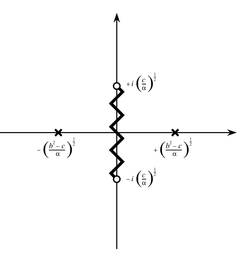
FIG. 1.: Analytic structure of $f(n)$ in the complex $n$ plane, showing the position of branch cuts and singularities for the case $b^{2}>c$.

Returning now to the full result of equation (55) we can now proceed to write down the thermodynamic potentials. Remembering that $\Gamma=-q=-\beta PV$, and using the volume of $S^{3}$, $V=2\pi^{2}a^{3}$, we can immediately write down the pressure (for $T>T_{c}$)

$$P= - \frac{1}{32\pi^{2}}c^{2}\ln(l^{2}c)+\frac{3c^{2}}{64\pi^{2}}$$ (66)

$$+ \frac{c^{2}}{\pi^{2}}\sum_{n=1}^{\infty}\frac{1}{\bigl{(}2\pi nac^{1\over 2}\bigr{)}^{2}}\left\{K_{2}\bigl{(}2\pi nac^{1\over 2}\bigr{)}-2\pi nac^{1\over 2}K_{3}\bigl{(}2\pi nac^{1\over 2}\bigr{)}\right\}$$ (67)

$$- \frac{1}{2\pi^{2}a^{3}\beta}\sum_{n=1}^{\infty}n^{2}\ln\left[\left(1-e^{-\beta(\omega_{n}+\mu)}\right)\left(1-e^{-\beta(\omega_{n}-\mu)}\right)\right].$$ (68)

The first few terms in the pressure are essentially unobservable renormalisation constants (since one can only really measure differences in pressure), and the last term is the term that one would predict from normal statistical mechanics. The Bessel function term, however, is observable since it varies with volume; it is a contribution to the pressure due to the Casimir effect. Notice (as one would expect) that it is independent of both the temperature and chemical potential - its origin is in the vacuum, not the finite temperature and chemical potential effects. Also, because of the asymptotic form of the Bessel functions, this term tends towards zero as the volume (and therefore $a$) tends to infinity; it will not survive the infinite volume limit.

Equation (68) on its own does not completely determine the pressure: $\mu$ is unknown. To rectify this, we must now consider the vacuum expectation value of the charge. Above the critical temperature it is given by (14)

$$Q = \sum_{n=1}^{\infty}{n^{2}\over e^{\beta(\omega_{n}+\mu)}-1}+\sum_{n=1}^{\infty}{n^{2}\over e^{\beta(\omega_{n}-\mu)}-1}$$ (69)

$$= \sum_{n=1}^{\infty}{2n^{2}\sinh(\beta\mu)e^{\beta\omega_{n}}\over\bigl{(}e^{\beta(\omega_{n}+\mu)}-1\bigr{)}\bigl{(}e^{\beta(\omega_{n}-\mu)}-1\bigr{)}}$$ (70)

The charge $Q$ is made up from two parts: one contribution from particles (chemical potential $\mu$), and a contribution from antiparticles (chemical potential $-\mu$). Its high temperature behaviour is examined in [12]. The low temperature behaviour ($\beta\to\infty$) would be trivial to calculate, except that a priori one can not be sure that (70) still holds.

If one plots (70) as a function of $\mu$ one obtains a graph similar to Fig. 2 .The charge diverges whenever $\mu$ tends to one of the $\omega_{n}$, and it is multivalued, being divided up into intervals by these values. Now from (70) $\mu$ and its’ derivatives are well defined within each of these intervals (since the sums are absolutely convergent) hence $\mu$ is a continuous function of $T$ in these regions. Furthermore, within each of these regions $Q$ takes on all values; hence after choosing one of these regions one can never evolve out of it by a change of $Q$ or $T$. Since a change of $Q\to-Q$ (i.e swapping particles with antiparticles) must cause $\mu\to-\mu$ only the first region is physical.

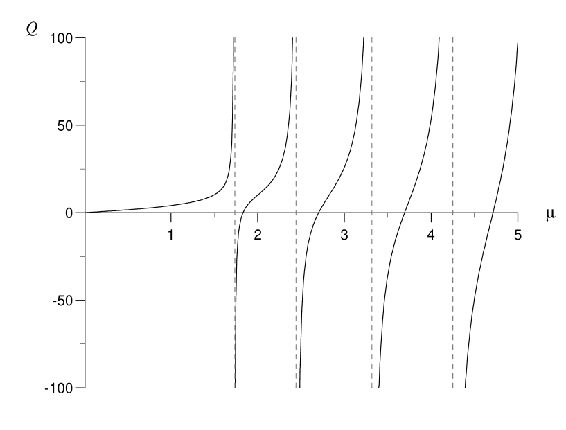
FIG. 2.: Plot of charge $Q$ against $\mu$.

Although we cannot solve for $\mu$ analytically, in the case of the Einstein Universe we have done so numerically. The results are shown in Fig. 3 (which uses the charge density $\rho=Q/V$ rather than $Q$. From the figure, one can see that in fact there is no critical temperature: $\mu$ tends towards its critical value, only reaching it at $T=0$. This is most marked in the case $a=0.25$. When the volume becomes large, the curve for $\mu$ starts to look more like the scenario given above and $\mu$ tends asymptotically to its critical value (but it still does not reach it until $T=0$). This means that the $\tilde{S}[\bar{\varphi}]$ term in $\Gamma$ is always zero : there is no symmetry breaking on the Einstein universe and hence BEC does not occur.

FIG. 3.: Plots of $\mu$ against Temperature. Curves have $m^{2}=2$ and $\xi=1/6$. The dotted line corresponds to $a=0.25$, the dashed line is $a=1.0$ and the solid line is $a=20$.

IV Finite Volume Spaces

In the previous section we examined numerically the Einstein static universe and showed that the critical temperature is zero, in contrast to calculations based on high temperature expansions (which implicitly assume that there is a non zero critical temperature!). We now wish to consider the generic case of a compact spatial manifold.

Usually in statistical mechanics, we are interested in the limit as both the volume and the number of particles tends to infinity. It is then meaningless to talk about $Q$, because if we imagine starting off at some low temperature with no anti-particles the charge will also become infinite. Thus we now restrict our attention to $\rho=Q/V$. For a general finite volume space, this will be given by (see appendix.A or [6])

$$\rho={2\sinh(\beta\mu)\over V}\sum_{n=1}^{\infty}{n^{2}e^{\beta\omega_{n}}\over\bigl{(}e^{\beta(\omega_{n}+\mu)}-1\bigr{)}\bigl{(}e^{\beta(\omega_{n}-\mu)}-1\bigr{)}}$$ (71)

where the $\omega_{n}$ satisfy $0<\omega_{1}<\omega_{2}\leq\omega_{3}\leq\ldots$   but are otherwise arbitrary.

The form of $\rho$ vs $\mu$ must be similar to fig.1: $\rho\to\infty$ whenever $\mu\to\omega_{n}$ and by similar arguments to those in section III $\mu$ lies in the region $|\mu|<\omega_{1}$ (the summand behaves like $\exp-\beta\omega_{n}$ as $\omega_{n}$ becomes large - which we expect to happen as $n\to\infty$ - therefore the sum is absolutely convergent). Thus we separate off the ground state contribution from $\rho$:

$$\rho={2\sinh(\beta\mu)e^{\beta\omega_{1}}\over\bigl{(}e^{\beta(\omega_{1}+\mu)}-1\bigr{)}\bigl{(}e^{\beta(\omega_{1}-\mu)}-1\bigr{)}}+\rho_{e}(\beta,\mu).$$ (72)

and we consider the situation when $\mu$ is close to its critical value. We will define $\mu=\omega_{1}-\delta$, $\delta<<1$. $\rho_{e}(\beta,\mu)$ can be interpreted as the charge density in excited states.

Here (72) is to be considered as an equation in the unknown $\mu$; $\rho$ is a measurable quantity which here we consider as fixed. Furthermore, all the equations which were used to derive (72) are well defined at every point except the critical value (ie are well defined for all $\delta\not=0$); thus no matter how close to the critical point we are, we must always be able to solve for $\mu$. But this is just the statement that the limit of the r.h.s of (72) exists as $\delta\to 0$ and is equal to $\rho$. Now $\rho_{e}(\beta_{c},\mu)$ tends to some limit, $\rho_{el}$ say, as $\delta\to 0$.(This must be true because the only divergent part is in the ground state; the sum in $\rho_{e}$ is absolutely convergent and therefore must sum to some value at $\mu=\omega_{1}$). Let us call the ground state contribution in (72) $\rho_{g}(\beta,\mu)$ and let us also define the constant $\rho_{l}=\rho-\rho_{el}$.

Assume that we have a critical point, ie a point where $\mu\to\omega_{1}$ as $\beta\to\beta_{c}$. Thus we must have that

$$\rho_{g}(\beta,\omega_{1}-\delta)\to\rho_{l}\quad\hbox{as $\delta\to 0$.}$$ (73)

But by expanding $\rho_{g}$ in terms of $\delta$, it is easy to show that

$$\rho_{g}\sim\frac{1}{\beta\delta V}+O\left(\frac{1}{V}\right)\quad\hbox{as $\delta\to 0$}$$ (74)

The only way that we can get a finite limit for $\rho$ as $\delta\to 0$ (and $\beta\to\beta_{c}$) is if $\beta V=O(1/\delta)$ as $\delta\to 0$.

For a finite volume space we must have $\beta=O(1/\delta)$ as $\delta\to 0$; thus $\beta\to 0$ as $\mu\to\omega_{1}$ and the critical temperature is zero. Since for all finite $\beta$, $\mu\not=\omega_{1}$ this also means that there can be no symmetry breaking in such spaces. However, as we saw in the Einstein universe, if the volume is large we expect that $\mu$ can be quite close to its critical value for some finite temperature; thus there will be a large number of particles in the ground state and the physics will look similar to the infinite volume physics. In this situation the temperature at which we expect some degree of condensation is at a critical temperature obtained by taking the infinite volume limit. Alternatively one can try to define the onset of condensation by looking for the maximum of the specific heat since this is the property which is usually searched for experimentally.

V Conclusion

We examined the Einstein static universe numerically, and showed that the critical temperature defined by $\mu\to\omega_{1}$ is zero in contrary to previous calculations. These gave the wrong result because they were based on high temperature expansions. We then generalized our result to arbitrary curved spaces of finite volume and showed that there is no symmetry breaking on these spaces at finite temperature and density.

A Non interacting scalar field at finite temperature

In this appendix we wish to show in detail how the generalised zeta function techniques reproduce the earlier results of [6]. Taking the field theory of section. II we define $\{\varphi_{n}\}$ s.t.

$$\bigl{(}-\nabla^{2}+m^{2}+U_{1}(x)\bigr{)}\varphi_{n}=\varepsilon^{2}_{n}\varphi_{n}.$$ (A1)

If we let $a=2\pi/\beta$ then

$$\zeta_{\cal G}(s)=\sum_{n}\sum_{j=-\infty}^{\infty}\left[(aj+i\mu)^{2}+\varepsilon^{2}\right]^{-s}$$ (A2)

where the sum over $n$ in (A2) is over all the eigenvalues of (A1). Using (24) and the Jacobi identity we obtain

$$\zeta_{\cal G}(s)=\frac{\pi^{1\over 2}}{a\Gamma(s)}\int_{0}^{\infty}dt\ t^{s-{3\over 2}}\left(\sum_{n}\exp(-\varepsilon^{2}_{n}t)\right)\left(1+2\sum_{j=1}^{\infty}\exp\left(-{j^{2}\pi^{2}\over a^{2}t}\right)\cosh\left({2\pi j\mu\over a}\right)\right)$$ (A3)

The integral in (A3) naturally splits up into two parts. In the second part, the integral is easily done using the Bessel function integral (by a change of variable $t\to\varepsilon_{n}^{2}t$):

$$\frac{2\pi^{1\over 2}}{a\Gamma(s)}\sum_{n}\sum_{j=1}^{\infty}\int_{0}^{\infty}\! dt t^{s-{3\over 2}}\exp\left(-\varepsilon_{n}^{2}t-{j^{2}\pi^{2}\over a^{2}t}\right)\cosh\left({2\pi j\mu\over a}\right)$$ (A4)

$$= \frac{4\pi^{1\over 2}}{a\Gamma(s)}\sum_{n}\sum_{j=1}^{\infty}\cosh\left({2\pi j\mu\over a}\right)\left({\pi j\over a}\right)^{s-{1\over 2}}\varepsilon_{n}^{{1\over 2}-s}K_{-s+{1\over 2}}\left({2\pi j\varepsilon_{n}\over a}\right).$$ (A5)

Differentiating this, then evaluating at $s=0$ we obtain (remembering (46) )

$$\frac{4\pi^{1\over 2}}{a}\sum_{n}\sum_{j=1}^{\infty}\cosh\left({2\pi j\mu\over a}\right)\left({a\over\pi j}\right)^{1\over 2} \!\!\!\!\!\!\varepsilon_{n}^{1\over 2}K_{1\over 2}\left({2\pi j\varepsilon_{n}\over a}\right)$$ (A6)

$$= 2\sum_{n}\sum_{j=1}^{\infty}\frac{1}{j}\cosh\left({2\pi j\mu\over a}\right)\exp\left(-{2\pi j\varepsilon_{n}\over a}\right)$$ (A7)

$$= -\sum_{n}\left\{\ln\bigl{(}1-e^{-\beta(\varepsilon_{n}+\mu)}\bigr{)}+\ln\bigl{(}1-e^{-\beta(\varepsilon_{n}+\mu)}\bigr{)}\right\}$$ (A8)

where we have used the fact that $\beta=2\pi/a$ and $\ln(1-x)=-\sum_{n=1}^{\infty}x^{n}$.

The first integral in (A3) is

$$\frac{\pi^{1\over 2}}{a\Gamma(s)}\sum_{n}\int_{0}^{\infty}dt\ t^{s-{3\over 2}}\exp\bigl{(}-\varepsilon_{n}^{2}t\bigr{)} = \frac{\pi^{1\over 2}}{a}\frac{\Gamma(s-{1\over 2})}{\Gamma(s)}\sum_{n}\frac{1}{\varepsilon_{n}^{2s-1}}$$ (A9)

$$= \frac{\pi^{1\over 2}}{a}\frac{\Gamma(s-{1\over 2})}{\Gamma(s)}\zeta_{\varepsilon_{n}^{2}}(s-1/2)$$ (A10)

We expect $\zeta_{\varepsilon_{n}^{2}}(s-1/2)$ to be an analytic function of $s$ except for a few simple poles. This implies that it has a well defined Laurent expansion about $s=0$, which we will write as

$$\zeta_{\varepsilon_{n}^{2}}\sim\frac{A_{-1}}{2s}+A_{0}+2A_{1}s+O(s^{2}).$$ (A11)

Note that $A_{-1}$ is the residue of the generalised zeta function, using as the eigenvalues $\varepsilon_{n}^{2}$, at the point $s=1/2$. This expansion, together with (46), immediately gives

$$\left.\pi^{1\over 2}\frac{\Gamma(s-{1\over 2})}{\Gamma(s)}\zeta_{\varepsilon_{n}}(s-1/2)\right|_{s=0}=\pi^{1\over 2}\Gamma\left(-{1\over 2}\right)A_{-1}=-2\pi A_{-1}.$$ (A12)

Also

$$\left[\pi^{1\over 2}\frac{\Gamma\left(s-{1\over 2}\right)}{\Gamma(s)}\zeta_{\varepsilon_{n}}(s-1/2)\right]^{\prime} \sim \pi^{1\over 2}\Gamma\left(s-{1\over 2}\right)\psi\left(s-{1\over 2}\right)A_{-1}$$ (A14)

$$+\ \pi^{1\over 2}\Gamma(s-{1\over 2})(A_{0}+\gamma)+O(s)\quad\hbox{as $s\to 0$,}$$

where $\psi(z)=\Gamma^{\prime}(z)/\Gamma(z)$.Making use of $\psi(-1/2)=-\gamma+2(1-\ln 2)$ and then substituting in (7) (remembering that the $\tilde{S}[\bar{\varphi}]$ term never appears - see section IV) gives

$$\Gamma=\beta A_{-1}\ln l^{2} + \beta\{(2-2\ln 2-\gamma)A_{-1}+A_{0}+\gamma\}$$ (A15)

$$+ \sum_{n}\ln\left[\left(1-e^{-\beta(\varepsilon_{n}+\mu)}\right)\left(1-e^{-\beta(\varepsilon_{n}-\mu)}\right)\right].$$ (A16)

By comparison with the result of Haber and Weldon [6], or from examination of (A1), we note that the ${\varepsilon}$ are the energy eigenvalues and identify

$$\sum_{n}\varepsilon_{n}=A_{-1}\ln l^{2}+\{(2-2\ln 2-\gamma)A_{-1}+A_{0}+\gamma\}$$ (A17)

which is essentially the (regularized) Casimir energy.

Now , because $\varepsilon_{n}^{2}=\sigma_{n}+m^{2}$,

$$\zeta_{\varepsilon_{n}} = \frac{1}{\Gamma(s)}\int_{0}^{\infty}dt\ t^{s-1}e^{-t(\sigma_{n}+m^{2})}$$ (A18)

$$= \frac{1}{\Gamma(s)}\int_{0}^{\infty}dt\ t^{s-1}e^{-m^{2}t}\Theta(t).$$ (A19)

It may be noted that $\Theta(t)$ is tr$\ \exp[-t(-\nabla^{2}+U_{1})]$ which has a known asymptotic expansion as $t\to 0$ namely,

$$\Theta(t)\simeq(4\pi t)^{-D/2}\sum_{k=0,1/2,1,\ldots}^{\infty}t^{k}\theta_{k}.$$ (A20)

The $\theta_{k}$ are the same coefficients that are used in [23], and depend only on the geometry and the conditions on the fields at the boundaries of $\Sigma$. (Typically they involve products of the curvature invariants and the masses of the fields on $\Sigma$.) $D$ is the dimension of $\Sigma$ and this is the only place in which it enters explicitly. Use of this expansion in (A19) together with expanding the $\exp(-m^{2}t)$ allows one to find

$$A_{-1}=\left\{{4\pi^{-D/2}\sum_{l=0}^{D/2}(-1)^{D/2-l}\theta_{1/2+l}\,m^{D-2l}\hbox{ for D even}\atop 4\pi^{-D/2}\sum_{l=0}^{(D+1)/2}(-1)^{(D+1)/2-l}\theta_{l}\,m^{D+1-2l}\hbox{ for D odd}}\right.$$ (A21)

Thus the residue of $\zeta_{\varepsilon_{n}}(0)$ exists and can be written down in general. As claimed earlier, one can see that it depends only on the geometry of the space. Unfortunately the authors are aware of no similar method for calculating $A_{0}$ in general, and one is reduced to working out the analytic continuation of $\zeta_{\varepsilon_{n}}$ case by case. However, since the statistical mechanical contribution can be written down explicitly, one only needs to focus on the zero temperature zeta functions.

B Antipodal Identification

A simple modification of the Einstein static universe is to identify antipodal points on $S^{3}$. Two cases are possible: periodic identification and antiperiodic identification of the fields. In the case of periodic identification, all the odd modes of $-\nabla^{2}$ must vanish. Thus the generalised zeta function in this case is

$$\zeta_{\lambda_{j,N}}=\sum_{j=-\infty}^{\infty}\sum_{N=0}^{\infty}{(2N+2)^{2}\over\left[\left({2\pi j\over\beta}+i\mu\right)^{2}+{(2N+1)(2N+3)\over a^{2}}+{6\xi\over a^{2}}+m^{2}\right]^{s}}.$$ (B1)

At first sight, it appears that we shall have to repeat the entire calculation for the zeta function above. However if one makes the change of variable, $n=N+1$, and notes that $(2N+1)(2N+3)=(2n-1)(2n+1)=4n^{2}-1$, we can rewrite (B1) as

$$\zeta_{\lambda_{j,n}} = \sum_{j=-\infty}^{\infty}\sum_{n=1}^{\infty}{4n^{2}\over\left[\left({2\pi j\over\beta}+i\mu\right)^{2}+{4n^{2}-1\over a^{2}}+{6\xi\over a^{2}}+m^{2}\right]^{s}}$$ (B2)

$$= 4\times\sum_{j=-\infty}^{\infty}\sum_{n=1}^{\infty}{n^{2}\over\left[(aj+ib)^{2}+\alpha n^{2}+c\right]^{s}},$$ (B3)

where $a=2\pi/\beta$, $\alpha=4/a^{2}$, $b=\mu$ and $c=(6\xi-1)/a^{2}$. This is the zeta function that we had before, and

$$\Gamma_{e}= \frac{1}{32}\beta a^{3}c^{2}\ln(l^{2}c)-\frac{3}{64}\beta a^{3}c^{2}$$ (B6)

$$-\beta a^{3}c^{2}\sum_{n=1}^{\infty}\frac{1}{\bigl{(}\pi nac^{1\over 2}\bigr{)}^{2}}\left\{K_{2}\bigl{(}\pi nac^{1\over 2}\bigr{)}-\pi nac^{1\over 2}K_{3}\bigl{(}\pi nac^{1\over 2}\bigr{)}\right\}$$

$$+4\sum_{n=1}^{\infty}n^{2}\ln\left[\left(1-e^{-\beta(\omega_{n}+\mu)}\right)\left(1-e^{-\beta(\omega_{n}-\mu)}\right)\right]$$

$\omega_{n}=\bigl{(}(2n/a)^{2}+c\bigr{)}$ and $c$ is as before. The factor of four in $\zeta$ appears simply because the space has half the volume that it had originally .As the volume becomes large we expect the log term in $\Gamma$ to also be directly proportional to the volume, which explains the four here (as the sum tends to an integral, the measure will give a term proportional to $a^{3}$. But in (B6) $a\to a/2$ compared to our original effective action, leaving us with an overall factor of two). The spacetime gives us an effective thermodynamic mass, $c$, identical to the value on $S^{3}$, however the detailed dependence of the sums at small volume is now radically different.

Because the expression (23) is an absolutely convergent double sum for all points at which it is defined, we can write

$$\zeta_{odd}=\zeta_{S^{3}}-\zeta_{even}$$ (B7)

which will be true even after analytic continuation.

Previously, it has been remarked that there would be many interesting properties of this space associated with the possibility of have a $x$ dependent charge density. However, this charge density appeared through the $\tilde{S}[\bar{\varphi}]$ term which we have seen will be absent.

REFERENCES

[1]L.D. Landau and E. M. Lifshitz, Statistical Physics.
(Pergammon,
London, 1969).
[2] R. K. Pathria, Statiscal Mechanics. (Pergammon,
London,
1972).