IASSNS-HEP-95/97

hep-th/9602045

(to appear in Physics Reports)

September 1996

String Theory and the Path to Unification:
A Review of Recent Developments
Keith R. Dienes
School of Natural Sciences, Institute for Advanced Study
Olden Lane, Princeton, N.J. 08540 USA

This is a pedagogical review article surveying the various approaches towards understanding gauge coupling unification within string theory. As is well known, one of the major problems confronting string phenomenology has been an apparent discrepancy between the scale of gauge coupling unification predicted within string theory, and the unification scale expected within the framework of the Minimal Supersymmetric Standard Model (MSSM). In this article, I provide an overview of the different approaches that have been taken in recent years towards reconciling these two scales, and outline some of the major recent developments in each. These approaches include string GUT models; higher affine levels and non-standard hypercharge normalizations; heavy string threshold corrections; light supersymmetric thresholds; effects from intermediate-scale gauge and matter structure beyond the MSSM; strings without supersymmetry; and strings at strong coupling.

1 Introduction

As is well-known, string theories achieve remarkable success in answering some of the most vexing problems of theoretical high-energy physics. With string theory, we now have for the first time a consistent theoretical framework which is finite and which simultaneously incorporates both quantum gravity and chiral supersymmetric gauge theories in a natural fashion. An important goal, therefore, is to determine the extent to which this framework is capable of describing other more phenomenological features of the low-energy world.

In this review article, I shall focus on one such feature: the unification of gauge couplings. There are various reasons why this is a particularly compelling feature to study. On the one hand, the unification of gauge couplings — like the appearance of gravity or of gauge symmetry in the first place — is a feature intrinsic to string theory, one whose appearance has basic, model-independent origins. On the other hand, viewing the situation from an experimental perspective, the unification of the gauge couplings is arguably the highest-energy phenomenon that any extrapolation from low-energy data can uncover; in this sense it sits at what is believed to be the frontier between our low-energy $SU(3)\times SU(2)\times U(1)$ world, and whatever may lie beyond. Thus, the unification of gauge couplings provides a fertile meeting-ground where string theory can be tested against the results of low-energy experimentation.

At first glance, string theory appears to fail this test: it predicts, a priori, a unification of gauge couplings at a scale $M_{\rm string}\approx 5\times 10^{17}$ GeV, approximately a factor of 20 higher than the expected scale $M_{\rm MSSM}\approx 2\times 10^{16}$ GeV obtained through extrapolations from low-energy data within the framework of the Minimal Supersymmetric Standard Model (MSSM). While this may seem to be a small difference in an absolute sense (amounting to only 10% of the logarithms of these mass scales), this discrepancy nevertheless translates into predictions for the low-energy gauge couplings that differ by many standard deviations from their experimentally observed values. This is therefore a major problem for string phenomenology.

Fortunately, there are various effects which may modify these naive predictions, and thereby reconcile these two unification scales. These include: the appearance of a possible grand-unified (GUT) symmetry at the intermediate scale $M_{\rm MSSM}$ (which would then unify with gravity and any other “hidden-sector” gauge symmetries at $M_{\rm string}$); the possibility that the MSSM gauge group is realized in string theory through non-standard higher-level affine gauge symmetries and/or exotic hypercharge normalizations (which would alter the boundary conditions of the gauge couplings at unification); possible large “heavy string threshold corrections” (which would effectively lower the predicted value of $M_{\rm string}$); possible effects due to light SUSY thresholds (arising from the breaking of supersymmetry at a relatively low energy scale); and the appearance of extra matter beyond the MSSM (as often arises in realistic string models). There even exist unification scenarios based on strings without spacetime supersymmetry, and on strings at strong coupling. It is presently unknown, however, which of these scenarios (or which combination of scenarios) can successfully explain the apparent discrepancy between $M_{\rm MSSM}$ and $M_{\rm string}$ in string theory. In other words, it is not known which “path to unification”, if any, string theory ultimately chooses.

In this article, I shall summarize the basic status of each of these possibilities, and outline some of the recent developments in each of these areas. As we shall see, some of these paths are quite feasible, and can actually reconcile string-scale unification with low-energy data. Others, by contrast, are tied to more subtle issues in string theory, and await further insight.

It is precisely for such reasons that this review has been written. Given the recent experimental results confirming gauge coupling unification within the MSSM, there is now considerable interest among low-energy phenomenologists in the potential that gauge coupling unification holds for uncovering and probing new physics at very high energy scales. It is therefore particularly important at this time to survey the possibilities for new physics that are suggested by string theory. But there are also string-based reasons why a current review should be particularly useful. Over the past decade, string model-building and string phenomenology have matured to the point that specific phenomenological issues such as gauge coupling unification can now be meaningfully and quantitatively addressed. Moreover, as we shall see, the past several years have witnessed an explosion in the development of different string-based unification scenarios, with ideas and results coming from many different directions. Indeed, each of these various “paths to unification” has now been investigated in considerable detail, and the relevant issues that are raised within each scenario have now been systematically explored. This review should therefore serve not only to organize and summarize the accomplishments achieved within each of these “paths to unification”, but also to point the way towards understanding how, through gauge coupling unification, the predictions of string theory may eventually have a direct bearing on low-energy physics.

This article is organized as follows. In Sect. 2, I review the basic problem of gauge coupling unification, and highlight some of the differences that exist between gauge coupling unification in field theory and in string theory. In Sect. 3, I then provide an outline of the various approaches that have been proposed for understanding gauge coupling unification in string theory. The seven sections which follow (Sects. 4 through 10) then discuss each of these approaches in turn, and survey their relevant issues, problems, and current status. In particular, Sect. 4 focuses on string GUT models; Sect. 5 deals with non-standard affine levels and hypercharge normalizations; Sect. 6 discusses heavy string threshold corrections; Sect. 7 analyzes light SUSY thresholds and intermediate-scale gauge structure; Sect. 8 considers extra matter beyond the MSSM; Sect. 9 introduces gauge coupling unification via strings without spacetime supersymmetry; and Sect. 10 outlines a proposal based on strings at strong coupling. Finally, in Sect. 11, I conclude with a brief summary and suggestions for further research.

Disclaimers

This review article is aimed at discussing recent progress in one specific area: the unification of gauge couplings within string theory. As such, this review does not attempt to cover the vast literature of field-theoretic unification models, nor (at the other end) does it attempt to discuss general aspects of string model-building or string phenomenology. For reviews of the former subject, the reader should consult Ref. [1]; likewise, for recent reviews of the latter subject, the reader is urged to consult Refs. [2, 3]. Although certain portions of this review are based upon research [4, 5, 6, 7] that I have performed in joint collaborations, I have nevertheless attempted to place these results in context by surveying related recent works by other authors as well. My hope is therefore that this article presents a fairly complete survey of the issues surrounding gauge coupling unification in string theory, including most lines of development that have been advanced through the present time (September 1996). Finally, since my goal has been to present a pedagogical and (hopefully) non-technical introduction to recent progress in this field, I have avoided the detailed mathematics that is involved in any particular approach. Therefore, for further details — or for applications to related issues beyond the scope of this review — the reader should consult the relevant references.

2 Background

2.1 The problem of gauge coupling unification

Figure 1: One-loop evolution of the gauge couplings within the (non-supersymmetric) Standard Model. Here $\alpha_{1}\equiv(5/3)\alpha_{Y}$, where $\alpha_{Y}$ is the hypercharge coupling in the conventional normalization. The relative width of each line reflects current experimental uncertainties.

Figure 2: One-loop evolution of the gauge couplings within the Minimal Supersymmetric Standard Model (MSSM), assuming supersymmetric thresholds at the $Z$ scale. As in Fig. 2, $\alpha_{1}\equiv(5/3)\alpha_{Y}$, where $\alpha_{Y}$ is the hypercharge coupling in the conventional normalization. The relative width of each line reflects current experimental uncertainties.

The Standard Model of particle physics is by now extremely well-established, and accounts for virtually all presently available experimental data. Moreover, one particular extension of the Standard Model, namely the Minimal Supersymmetric Standard Model (MSSM) [8], successfully incorporates the Standard Model within the framework of a supersymmetric theory, thereby improving the finiteness properties of the theory and providing, for example, an elegant solution to the technical gauge hierarchy problem.

This introduction of $N=1$ supersymmetry, however, also has another profound effect: it brings about a unification of the gauge couplings, as illustrated in Figs. 2 and 2. This unification can be seen as follows. At the $Z$ scale $M_{Z}\approx 91.16$ GeV, the experimentally accepted values for the hypercharge, electroweak, and strong gauge couplings are respectively given (within the $\overline{\rm MS}$ renormalization group scheme) as [9]

$$\alpha_{Y}^{-1}(M_{Z})|_{\overline{\rm MS}} \equiv 98.29\pm 0.13$$

$$\alpha_{2}^{-1}(M_{Z})|_{\overline{\rm MS}} \equiv 29.61\pm 0.13$$

$$\alpha_{3}^{-1}(M_{Z})|_{\overline{\rm MS}} \equiv 8.3\pm 0.5~{}$$ (2.1)

where $\alpha_{i}\equiv g_{i}^{2}/(4\pi)$ for $i=Y,2,3$. In Eq. (2.1) we have assumed the conventional hypercharge normalization in which the Standard Model right-handed singlet electron state $e_{R}$ has unit hypercharge. We then extrapolate these couplings to higher energy scales $\mu$ via the standard one-loop renormalization group equations (RGE’s) of the form

$$\alpha_{i}^{-1}(\mu)~{}=~{}\alpha_{i}^{-1}(M_{Z})~{}-~{}{b_{i}\over 4\pi}\,\ln\,{\mu^{2}\over M_{Z}^{2}}~{}.$$ (2.2)

Note that the one-loop beta-function coefficients $b_{i}$ that govern this logarithmic running depend on the matter content of the theory. It is therefore here that the introduction of $N=1$ supersymmetry plays a role (i.e., by introducing superpartner states and an extra Higgs doublet into the theory). Specifically, one finds that these coefficients take the values

$$(b_{Y},b_{2},b_{3})~{}=~{}\cases{~{}(7,-3,-7)&within the Standard Model\cr~{}(11,1,-3)&within the MSSM.\cr}$$ (2.3)

Using the beta-function coefficients $b_{i}$ of the Standard Model and extrapolating the low-energy couplings upwards according to Eq. (2.2), one then finds that the three gauge couplings fail to meet at any scale. This is illustrated in Fig. 2. By contrast, performing this extrapolation within the MSSM, one discovers [1] an apparent unification of gauge couplings of the form

$${5\over 3}\,\alpha_{Y}(M_{\rm MSSM})~{}=~{}\alpha_{2}(M_{\rm MSSM})~{}=~{}\alpha_{3}(M_{\rm MSSM})~{}\approx~{}{1\over 25}~{}$$ (2.4)

at the scale

$$M_{\rm MSSM}~{}\approx~{}2\,\times\,10^{16}~{}{\rm GeV}~{}.$$ (2.5)

This situation is shown in Fig. 2. The fact that the gauge couplings unify within the MSSM is usually interpreted as evidence not only for $N=1$ supersymmetry, but also for the existence of a single large grand-unified gauge group $G_{\rm GUT}$ which breaks to $SU(3)\times SU(2)\times U(1)_{Y}$ at the MSSM scale $M_{\rm MSSM}$. Indeed, with this interpretation, even the factor of $5/3$ appearing in Eq. (2.4) has a natural explanation, for it essentially represents the group-theoretic factor by which the conventional hypercharge generator must be rescaled in order to be unified along with the $SU(2)$ and $SU(3)$ generators within a single non-abelian group $G_{\rm GUT}$ such as $SU(5)$, $SO(10)$, or $E_{6}$.

Thus, the popular field-theoretic scenario that is currently envisioned is as follows. At high energies far above $M_{\rm MSSM}$, we have $N=1$ supersymmetry and some grand-unified group $G_{\rm GUT}$, with all matter falling into supersymmetric representations of this group. Then, at the MSSM scale, this group is presumed to break directly to $SU(3)\times SU(2)\times U(1)_{Y}$, and any extra states that do not appear within the MSSM will have masses near $M_{\rm MSSM}$ and thus not affect the running of gauge couplings below this scale. The MSSM itself is then presumed to govern physics all the way down to the scale $M_{\rm SUSY}$ at which SUSY-breaking occurs, and then finally, below $M_{\rm SUSY}$, we expect to see merely the Standard-Model gauge group and spectrum. The scale $M_{\rm SUSY}$ is set, of course, with two considerations in mind: it must be sufficiently high to explain why the lightest superparticles have not yet been observed, and it must be sufficiently low that the gauge hierarchy is protected. This in turn constrains various measures of SUSY-breaking, such as the value of the mass supertrace ${\rm Str}(M^{2})$.

On the face of it, this is a fairly compelling picture. There are, however, a number of outstanding problems that are not addressed within this scenario. First, the unification scale $M_{\rm MSSM}$ is quite close to the Planck scale $M_{\rm Planck}=\sqrt{1/G_{N}}\approx 10^{19}$ GeV, yet gravity is not incorporated into this picture. Second, one would hope to explain the spectrum of the Standard Model and the MSSM, in particular the values of the many arbitrary free parameters which describe the fermion masses and couplings. Indeed, one might even seek an explanation of more basic parameters such as the number of generations or even the choice of gauge group. Third, if we truly expect some sort of GUT theory above $M_{\rm MSSM}$, we face the problem of the proton lifetime; stabilizing the proton requires a successful doublet-triplet splitting mechanism. Finally, we may even ask why we should expect a GUT theory at all. After all, the appearance of a grand-unified theory is essentially a theoretical prejudice, and is not required in any way for the theoretical consistency of the model. In other words, the unification of gauge couplings may just be a happy accident.

2.2 String theory vs. field theory

String theory, however, has the potential to address all of these shortcomings. First, it naturally incorporates quantum gravity, in the sense that a spin-two massless particle (the graviton) always appears in the string spectrum. Second, $N=1$ supersymmetric field theories with non-abelian gauge groups and chiral matter naturally appear as the low-energy limits of a certain phenomenologically appealing class of string theories (the heterotic strings) [11]. Third, such string theories may in principle provide a uniform framework for understanding all of the features of low-energy phenomenology, such as the appearance of three generations, the fermion mass matrices, and even a doublet-triplet splitting mechanism [12]. Indeed, string theories ultimately contain no free parameters!

But most importantly for the purposes of this article, string theories also imply a natural unification of the couplings. Indeed, regardless of the particular string model in question and independently of whether there exists any unifying GUT gauge symmetry in the model, it turns out that the gauge and gravitational couplings in heterotic string theory always automatically unify at tree-level to form one dimensionless coupling constant $g_{\rm string}$ [13]:

$$8\pi{G_{N}\over\alpha^{\prime}}~{}=~{}g_{i}^{2}\,k_{i}~{}=~{}g_{\rm string}^{2}~{}.$$ (2.6)

This unification relation holds because the gravitational and gauge interactions all arise from the same underlying sectors in the heterotic string, and can therefore be related to each other. Here $G_{N}$ is the gravitational coupling (Newton’s constant); $\alpha^{\prime}$ is the Regge slope (which sets the mass scale for excitations of the string); $g_{i}$ is the gauge coupling for each gauge group factor $G_{i}$; and $k_{i}$, which appears as the corresponding normalization factor for the gauge coupling $g_{i}$, is the so-called affine level (also often called the Kač-Moody level) at which the group factor $G_{i}$ is realized.

These affine levels have a simple origin in string theory, and can be understood as follows. In (classical) heterotic string theory, all gauge symmetries are ultimately realized in the form of worldsheet affine Lie algebras with central extensions [14]. Explicitly, this means that if one computes the operator product expansions (OPE’s) between the worldsheet currents $J^{a}(z)$ corresponding to any non-abelian group factor $G_{i}$ appearing in a given string model, one obtains a result of the form

$$J^{a}(z)J^{b}(w)~{}\sim~{}{if^{abc}\over z-w}\,J^{c}(w)~{}+~{}k\,{\vec{\alpha}_{h}^{2}\over 2}\,{\delta^{ab}\over(z-w)^{2}}~{}+~{}...$$ (2.7)

Here $f^{abc}$ are the structure constants of the Lie algebra, and $\vec{\alpha}_{h}^{2}$ is the squared length of the longest root $\vec{\alpha}_{h}$. While the first term in Eq. (2.7) has the expected form of the usual Lie algebra, the second term (the so-called “central extension”) appears as double-pole Schwinger contact term. As indicated in Eq. (2.7), the “level” $k$ is then defined as the coefficient of this double-pole term, and the gauge symmetry is said to have been “realized at level $k$”. (The specific definition of $k$ in the case of abelian groups will be presented in Sect. 5.1.) Current-algebra relations of the form in Eq. (2.7) are those of so-called affine Lie algebras, which are also often called Kač-Moody algebras in the physics literature. Such algebras were first discovered by mathematicians in Ref. [15], and later independently by physicists in Ref. [16]. The affine levels $k$ that concern us here were first discovered in Ref. [16]. Note that the length $\vec{\alpha}_{h}^{2}$ is inserted into the definition in Eq. (2.7) so that the level $k$ is invariant under trivial rescalings of the currents $J^{a}(z)$. For non-abelian gauge groups, it turns out that the levels $k$ are restricted to be positive integers, while for $U(1)$ gauge groups they can take arbitrary model-dependent values.

We see, then, that string theory appears to give us precisely the features we want, with a prediction for the unification of the couplings in Eq. (2.6) that is strikingly reminiscent of the “observed” MSSM unification in Eq. (2.4). There are, however, some crucial differences between the unification of gauge couplings in field theory and in string theory. First, string theory, unlike field theory, is intrinsically a finite theory; thus when we talk of a running of the gauge couplings in string theory, we are implicitly calculating within the framework of the low-energy effective field theory which is derived from only the massless (i.e., observable) states of the full string spectrum. Second, again in contrast to field theory, in string theory all couplings are actually dynamical variables whose values are fixed by the expectation values of certain moduli fields. For example, the string coupling $g_{\rm string}$ is related at tree-level to the VEV of a certain modulus, the dilaton $\phi$, via a relation of the form $g_{\rm string}\sim e^{-\langle\phi\rangle}$ [17]. These moduli fields — which are massless gauge-neutral Lorentz-scalar fields — essentially parametrize an entire space of possible ground states (or “vacua”) of the string, and have an effective potential which is classically flat and which remains flat to all orders in perturbation theory. For this reason one does not know, a priori, the value of the string coupling $g_{\rm string}$ at unification, much less the true string ground state from which to perform our calculations in the first place.

A third distinguishing feature between field-theoretic and string-theoretic unification concerns the presence of the affine levels $k_{i}$ in the unification relation (2.6). It is clear from Eqs. (2.6) and (2.7) that these factors essentially appear as normalizations for the gauge couplings $g_{i}$ (or equivalently for the gauge symmetry currents $J_{a}$), and indeed such normalizations are familiar from ordinary field-theoretic GUT scenarios such as those based on $SU(5)$ or $SO(10)$ embeddings in which the hypercharge generator $Y$ must be rescaled by a factor $k_{Y}=5/3$ in order to be unified within the larger GUT symmetry group. The new feature from string theory, however, is that such normalizations $k_{i}$ now also appear for the non-abelian gauge factors as well. We shall see, however, that the most-easily constructed string models have $k_{i}=1$ for the non-abelian gauge factors.

But once again, for the purposes of this article, the most important difference between gauge coupling unification in field theory and string theory is the scale of the unification. As we have already discussed, in field theory this scale is determined via an extrapolation of the measured low-energy couplings within the framework of the MSSM, ultimately yielding $M_{\rm MSSM}\equiv 2\times 10^{16}$ GeV. This number, deduced on the basis of experimental measurement of the low-energy couplings, appears without theoretical justification. In string theory, by contrast, the scale of unification $M_{\rm string}$ is fixed by the intrinsic scale of the theory itself. Since string theory is a theory of quantum gravity, its natural scale $M_{\rm string}$ is ultimately related to the Planck scale

$$M_{\rm Planck}~{}=~{}\sqrt{1/G_{N}}~{}\approx~{}1.22\times 10^{19}~{}{\rm GeV}~{},$$ (2.8)

and is given by

$$M_{\rm string}~{}=~{}g_{\rm string}\,M_{\rm Planck}~{}\sim~{}\sqrt{1/\alpha^{\prime}}$$ (2.9)

where $g_{\rm string}$ is the string coupling. For realistic string models, the string coupling $g_{\rm string}$ should be of order one at unification; this is not only necessary for rough agreement with experiment at low energies, but also guarantees that the effective four-dimensional field theory will be weakly coupled [18], making a perturbative analysis appropriate. At tree-level, therefore, $M_{\rm string}$ is the scale at which the unification in Eq. (2.6) is expected to take place. One-loop string effects have the potential to lower this scale somewhat, however, and indeed one finds [19] that in the $\overline{\rm DR}$ renormalization scheme, the scale of string unification is shifted down to

$$M_{\rm string} = {e^{(1-\gamma)/2}\,3^{-3/4}\over 4\pi}\,g_{\rm string}\,M_{\rm Planck}$$ (2.10)

$$\approx g_{\rm string}\,\times\,5.27\,\times\,10^{17}~{}~{}{\rm GeV}~{}$$

where $\gamma\approx 0.577$ is the Euler constant. Thus, assuming that $g_{\rm string}\sim{\cal O}(1)$ at unification, we have

$$M_{\rm string}~{}\approx~{}5\,\times\,10^{17}~{}~{}{\rm GeV}~{}.$$ (2.11)

We thus see that a factor of approximately 20 or 25 separates the predicted string unification scale from the MSSM unification scale. Equivalently, the logarithms of these scales (which are arguably the true measure of this discrepancy) differ by about 10% of their absolute values.

Figure 3: The fundamental problem of gauge coupling unification within string theory: the scale $M_{1}\equiv M_{\rm MSSM}\approx 2\times 10^{16}$ GeV at which the gauge couplings are expected to unify within the MSSM is significantly below the scale $M_{2}\equiv M_{\rm string}\approx 5\times 10^{17}$ GeV at which string theory predicts their unification with each other and with the gravitational coupling (Newton constant) $G_{N}$.

This situation is sketched in Fig. 3, where we compare the lower scale $M_{1}\equiv M_{\rm MSSM}$ at which the extrapolated gauge couplings unify with the higher scale $M_{2}\equiv M_{\rm string}$ at which string theory predicts their unification with each other and with the gravitational coupling $G_{N}$. There are several important comments to make regarding this figure. First, since $G_{N}$ has mass dimension $-2$, its running is dominated by classical effects which are stronger than the purely quantum-mechanical running experienced by the dimensionless gauge couplings $\alpha_{i}$. In order to see this explicitly, let us first recall that the dimensionless gauge couplings experience a scale dependence of the form $\alpha_{i}^{-1}(\mu)\sim\mu^{f_{i}}\tilde{\alpha}_{i}^{-1}$ where $\tilde{\alpha}_{i}$ are fixed numbers describing the strength of the gauge couplings, and where the functions $f_{i}$ (which are similar to anomalous dimensions) describe the quantum-mechanical scale-dependence of the gauge couplings. It is, of course, the scale-dependent quantities $\alpha_{i}^{-1}(\mu)$ that we have been considering all along, and we see that if we relate $\alpha_{i}^{-1}(\mu)$ to $\alpha_{i}^{-1}(M_{Z})$ by expanding $f_{i}$ to first order in the gauge couplings via $f_{i}=b_{i}\alpha_{i}(M_{Z})/2\pi+...$, we reproduce the one-loop renormalization group equations given in Eq. (2.2). The situation for the gravitational coupling is similar. We first define an analogous dimensionless gravitational coupling $G_{N}^{-1}(\mu)\sim\mu^{-2+f_{G}}\tilde{G}_{N}^{-1}$ where $\tilde{G}_{N}$ is the usual fixed dimensionful gravitational coupling (Newton constant), and where the two terms in the exponent $-2+f_{G}$ respectively represent the classical and quantum-mechanical contributions to the running. It is appropriate to consider this dimensionless gravitational coupling $G_{N}^{-1}(\mu)$ rather than $\tilde{G}_{N}^{-1}$ since it is $G_{N}^{-1}(\mu)$ which represents the effective strength of the gravitational interaction at the scale $\mu$. Since $f_{G}$ is proportional to $G_{N}$ and is therefore exceedingly small at energies below the Planck scale, we can disregard $f_{G}$ entirely and concentrate on the classical contribution. This yields the power-law scale dependence $G_{N}^{-1}(\mu)/G_{N}^{-1}(M_{Z})=(M_{Z}/\mu)^{2}$, which gives rise to an exponential curve when sketched relative to a logarithmic mass scale as in Fig. 3. In this context, it is also interesting to note that any possible unification of gauge and gravitational couplings must necessarily take the form $G_{N}(\mu)=\alpha_{i}(\mu)$ (where we are neglecting overall numerical factors), since only couplings of similar mass dimensionalities can be equated. Upon comparison with the string-theoretic tree-level unification prediction in Eq. (2.6), we then immediately find that such a unification is possible only when $\mu\sim 1/\sqrt{\alpha^{\prime}}\sim M_{\rm string}$. Thus, because string theory essentially relates a dimensionless gauge coupling to a dimensionful gravitational coupling, it has the property that the unification relation itself predicts the unification scale. Of course, the result $\mu\sim M_{\rm string}$ is merely the tree-level result, while the one-loop corrected unification scale is given in Eq. (2.10). Finally, also note that for illustrative purposes we have greatly exaggerated the difference between $M_{\rm MSSM}$ and $M_{\rm string}$ in this sketch.

Figure 4: Dependence on the string scale: the predicted value of the low-energy electroweak mixing angle $\sin^{2}\theta_{W}(M_{Z})$, assuming unification at $M_{\rm string}$. Results for both one-loop and two-loop running are plotted.

Figure 5: Dependence on the string scale: the predicted value of the low-energy coupling $\alpha_{\rm strong}(M_{Z})$, assuming unification at $M_{\rm string}$. Results for both one-loop and two-loop running are plotted.

One may argue that this discrepancy between the two unification scales is not a major problem, since it is only a 10% effect in terms of their logarithms. More generally, one may also argue that it is improper to worry about a discrepancy between scales of unification, since such scales are dependent upon the particular renormalization scheme employed, and hence have no physical significance. Both of these observations are of course true, but the gauge couplings themselves are physical quantities, and this discrepancy between $M_{\rm string}$ and $M_{\rm MSSM}$ implies that the hypothesis of string-scale unification yields incorrect values for low-energy couplings. In other words, if we take the predictions of string theory seriously and assume that the gauge couplings unify at $M_{\rm string}$ rather than at $M_{\rm MSSM}$, we find that a straightforward extrapolation down to low energies does not reproduce the correct values for these couplings at the $Z$ scale.

In order to appreciate the seriousness of this problem, recall that the experimentally measured values for these couplings at the $Z$ scale $M_{Z}\approx 91$ GeV in the $\overline{\rm MS}$ renormalization scheme were given in Eq. (2.1). Because the value of the electromagnetic coupling $\alpha_{\rm e.m.}(M_{Z})=1/127.9$ is known with great precision and is trivially related to the electroweak couplings $(\alpha_{Y},\alpha_{2})$ via the electroweak mixing angle

$$\alpha_{Y}^{-1} = \alpha_{\rm e.m.}^{-1}\,\cos^{2}\theta_{W}$$

$$\alpha_{2}^{-1} = \alpha_{\rm e.m.}^{-1}\,\sin^{2}\theta_{W}~{},$$ (2.12)

it is traditional to take $\alpha_{\rm e.m.}(M_{Z})$ as a fixed input parameter and quote the values of $(g_{Y},g_{2})$ in terms of the single electroweak mixing angle $\sin^{2}\theta_{W}$. Indeed, using Eq. (2.1), we then obtain the low-energy coupling parameters

$$\sin^{2}\theta_{W}(M_{Z})|_{\overline{\rm MS}} = 0.2315\pm 0.001~{}$$

$$\alpha_{3}(M_{Z})|_{\overline{\rm MS}} = 0.120\pm 0.010~{},$$ (2.13)

and we shall see later that conversion from the $\overline{\rm MS}$ scheme to the $\overline{\rm DR}$ scheme makes only a very small correction. By contrast, in Figs. 5 and 5 we have plotted the values of the same low-energy coupling parameters that one would obtain by assuming unification at different hypothetical values of $M_{\rm string}$, and then running down to low energies according to both one-loop and two-loop analyses within the MSSM. It is clear that for $M_{\rm string}$ taking the value indicated in Eq. (2.11), the predicted values of $\sin^{2}\theta_{W}(M_{Z})$ and $\alpha_{3}(M_{Z})$ deviate by many standard deviations from those that are measured. Thus, what may have seemed to be a minor discrepancy between two unification scales becomes in fact a major problem for string phenomenology.

3 Possible Paths to String-Scale Unification

Faced with this situation, a number of possible “paths” towards reconciliation have been proposed. We shall here summarize the basic features of each path, and devote the following sections to more detailed examinations of the issues involved in each.

3.1 Overview of possible paths

• String GUT models:  Perhaps the most obvious path towards reconciling the scale of string unification $M_{\rm string}$ with the apparent unification scale $M_{\rm MSSM}$ is through the assumption of an intermediate-scale unifying gauge group $G$, so that $SU(3)\times SU(2)\times U(1)_{Y}\subset G$. In this scenario, the gauge couplings would still unify at the intermediate scale $M_{\rm MSSM}$ to form the coupling $g_{G}$ of the intermediate group $G$, but then $g_{G}$ would run up to the string scale $M_{\rm string}$ where it would then unify, as required, with the gauge couplings of any other (“hidden”) string gauge groups and with the gravitational coupling. As far as string theory is concerned, this basic path to unification has two possible sub-paths, depending on whether the GUT group $G$ is simple [as in $SU(5)$ or $SO(10)$], or non-simple [as in the Pati-Salam unification scenario with $G=SO(6)\times SO(4)$, or the flipped $SU(5)$ scenario with $G=SU(5)\times U(1)$]. We shall refer to the first path as the “strict GUT” path, and the second as merely involving “intermediate-scale gauge structure”. As we shall see, these two sub-paths have drastically different stringy consequences and realizations.

• Non-standard affine levels and hypercharge normalizations:  A second possible path to unification retains the MSSM gauge structure all the way up to the string scale, and instead exploits the fact that in string theory, the hypercharge normalization $k_{Y}$ need not have the standard value $k_{Y}=5/3$ that it has in those GUT scenarios which make use of $SU(5)$ or $SO(10)$ embeddings. Indeed, in string theory, the value that $k_{Y}$ may take is a priori arbitrary. Likewise, in all generality, the affine levels $(k_{2},k_{3})$ that describe the non-abelian group factors $SU(2)$ and $SU(3)$ of the MSSM may also differ from their “usual” value $k_{2}=k_{3}=1$, and therefore it is possible that by building string models which realize appropriately chosen non-standard values of $(k_{Y},k_{2},k_{3})$, one can alter the running of the corresponding couplings in such a way as to realize gauge coupling unification at $M_{\rm string}$ while simultaneously obtaining the proper values of the low-energy parameters $\alpha_{\rm strong}$ and $\sin^{2}\theta_{W}$. Thus, this possibility would represent a purely string-theoretic effect. As we shall discuss, however, it remains an open question whether realistic string models with the required values of $(k_{Y},k_{2},k_{3})$ can be constructed.

• Heavy string threshold corrections:  The next three possible paths to string-scale unification all involve adding various “correction terms” to the renormalization group equations (RGE’s) of the MSSM. For example, the next possible path we shall discuss involves the so-called heavy string threshold corrections which represent the contributions from the infinite towers of massive (i.e., Planck-scale) string states that are otherwise neglected in an analysis of the purely low-energy massless string spectrum. Strictly speaking, such corrections must be included in any string-theoretic analysis, and it is possible that these corrections may be sufficiently large to reconcile string-scale unification with the observed low-energy couplings. Thus, like the non-standard affine levels and hypercharge normalizations, this too represents a purely stringy effect that would not arise in ordinary field-theoretic scenarios.

• Light SUSY thresholds:  A fourth possible path to unification involves the corrections due to light SUSY-breaking thresholds near the electroweak scale. While the plot in Fig. 2 assumes that the superpartners of the MSSM states all have equal masses at $M_{Z}$, it is expected that realistic SUSY-breaking mechanisms will yield a somewhat different sparticle spectroscopy. The light SUSY-breaking thresholds are the corrections that would be needed in order to account for this, and are typically analyzed in purely field-theoretic terms.

• Extra non-MSSM matter:  A fifth possible path towards reconciling the string unification scale with the MSSM unification scale involves the corrections due to possible extra exotic matter beyond the MSSM. Although introducing such additional matter is completely ad hoc from the field-theoretic point of view, such matter appears naturally in many realistic string models, and is in fact required for their self-consistency. Such matter also has the potential to significantly alter the naive string predictions of the low-energy couplings, and its effects must therefore be included.

• Strings without supersymmetry:  Another possible path towards unification, one which is highly unconventional and which lies outside the paradigm of the MSSM, involves strings without supersymmetry — i.e., strings which are non-supersymmetric at the Planck scale. Such string models therefore seek to reproduce the Standard Model, rather than the MSSM, at low energies. As a result of the freedom to adjust the hypercharge normalization that exists within the string framework, it turns out that gauge coupling unification can still be achieved in such models, even without invoking supersymmetry. Moreover, the scale of gauge coupling unification in this scenario surprisingly turns out to be somewhat closer to the string scale than it is within the MSSM.

• Strings at strong coupling:  Finally, there also exists another possible path to unification which — unlike those above — is intrinsically non-perturbative, and which makes use of some special features of the strong-coupling behavior of strings in ten dimensions.

   

   

   

Figure 6: Various paths to unification, as discussed in the text. Each path provides a different solution to the fundamental problem posed in Fig. 3.

The above “paths to unification” are clearly very different from each other, and thus imply different resolutions to the fundamental problem posed in Fig. 3. In Fig. 6, we have sketched some of these different resolutions; we remind the reader that once again these sketches are greatly exaggerated and are meant only to illustrate the basic scenarios. First, in Fig. 6(a), we illustrate the standard GUT resolution in which the three low-energy couplings emerge at $M_{1}\equiv M_{\rm MSSM}$ from a common GUT coupling which in turn unifies with the gravitational coupling at $M_{2}\equiv M_{\rm string}$. In Fig. 6(b), by contrast, we illustrate the approach based on modifications of the levels $k_{i}$. [Recall that in all of these sketches we are actually plotting not $\alpha_{i}^{-1}$ but $(k_{i}\alpha_{i})^{-1}$.] It is already clear from this sketch that successful string-scale unification generally requires decreasing $k_{Y}$ and increasing $k_{3}$; for convenience we have held $k_{2}$ constant in this plot. Next, in Fig. 6(c), we sketch the scenario based on heavy string threshold corrections. In this scenario, the exact tree-level unification relation (2.6) at $M_{\rm string}$ is corrected by fixed thresholds $\Delta_{i}$ which must have specific sizes and signs if they are to consistent with the observed gauge coupling unification at $M_{\rm MSSM}$. For example, it is already clear that we would require $\Delta_{1}-\Delta_{2}$ to be negative and $\Delta_{3}-\Delta_{2}$ to be positive.

The remaining sketches show the influence of possible non-trivial physics at intermediate scales $M_{i}$ between $M_{Z}$ and $M_{\rm MSSM}$. In Fig. 6(d), for example, we illustrate a scenario based on possible intermediate-scale gauge structure [such as, e.g., $SO(6)\times SO(4)$]. In such scenarios, the low-energy gauge couplings emerge only at the intermediate scale $M_{i}$ at which the larger gauge symmetry is broken, and the $U(1)$ gauge coupling generally experiences a discontinuity. Likewise, in Figs. 6(e) and 6(f), we show the effects of extra matter beyond the MSSM. In Fig. 6(e), we illustrate the effects of potential extra color triplets and electroweak doublets appearing at intermediate scales $M_{i}$ and $M^{\prime}_{i}$ respectively; for simplicity we have assumed that these extra states have vanishing hypercharge. It is clear that the effect of such extra matter states is essentially that of a corrective lens which “refocuses” the running of the gauge couplings so that they meet at $M_{\rm string}$ rather than at $M_{\rm MSSM}$. (Light SUSY thresholds also have a similar effect.) In Fig. 6(f), by contrast, we show the effect of extra matter in complete GUT multiplets. While such multiplets do not affect the unification scale to one-loop order, we have sketched a scenario in which they raise the unified coupling to such an extent that two-loop effects may become significant and then refocus the unification scale up to the string scale.

It is also possible to sketch the two remaining “paths to unification” that we have mentioned above. In particular, the scenario based upon strings without supersymmetry will be illustrated in Sect. 9 (see Fig. 15 for a precise plot), while the scenario based upon string non-perturbative effects is much more subtle, and essentially weakens the string unification predictions in such a way that the unification scale for the gauge couplings need no longer coincide with the string scale derived from the gravitational coupling. Thus, in this scenario, the original mismatch illustrated in Fig. 3 would continue to apply, but would no longer be viewed as problematic.

3.2 Choosing between the paths: General remarks

Given these many potential “paths to unification”, we are then left with one over-riding question: Which path to string-scale gauge coupling unification does string theory actually take? Or equivalently, we may ask: To what extent can realistic string models be constructed which exploit each of these possibilities?

These questions are far more subtle in string theory than they would be in ordinary field theory. Indeed, in field theory, it would not seem to be too difficult to construct models which exploit the GUT mechanism, or which introduce extra matter beyond the MSSM. In string theory, however, the situation is far more complicated because these different paths are often related to each other in deep ways that are not always immediately apparent. For example, as we shall see, any consistent realization of a “strict GUT” string model requires that the GUT gauge symmetry $G$ be realized with an affine level $k_{G}>1$. Likewise, the presence of non-standard hypercharges $k_{Y}$ in string theory can be shown to imply the existence of certain classes of exotic non-MSSM matter with fractional electric charge. Thus, the different “paths to unification” as we have outlined them are not independent of each other, and we expect that various combinations of all of these effects will play a role in different types of string models.

It is important to understand why such such unexpected connections arise in string theory, and why such seemingly disparate features such as affine levels, extra non-MSSM matter, and GUT gauge groups are all ultimately tied together. These connections essentially occur because the fundamental object in string theory is the string itself. Each of the different worldsheet modes of excitation of the string corresponds to a different particle in spacetime. Thus, in string theory, four-dimensional spacetime physics is ultimately the consequence of two-dimensional worldsheet physics. This means that the four-dimensional particle spectra, gauge symmetries, couplings, etc., that we obtain in a given string model are all ultimately determined and constrained by worldsheet symmetries.

There are numerous well-known examples of this interplay between worldsheet and spacetime physics, examples in which a given worldsheet symmetry has profound effects in spacetime. For example, worldsheet conformal invariance sets the spacetime Hagedorn temperature of the theory (with ensuing consequences in string thermodynamics), and establishes a critical spacetime dimension which is, in general, greater than four. It is this which necessitates a compactification to four dimensions, leading to an infinite moduli space of possible phenomenologically distinct string ground states. Likewise, worldsheet supersymmetry also has profound effects in spacetime: it introduces spacetime fermions into the string spectrum, lowers the critical spacetime dimension from 26 to 10, and sets an upper limit of 22 on the rank of the corresponding gauge group in a classical heterotic string. Even more profound are the effects of worldsheet modular invariance (or one-loop conformal anomaly cancellation): in certain settings this removes the tachyon from the spacetime string spectrum, introduces spacetime supersymmetry, and guarantees the ultraviolet finiteness of string one- and multi-loop amplitudes. Indeed, modular invariance is also responsible for the appearance of so-called GSO projections which remove certain states from all mass levels of the string spectrum, and likewise requires the introduction of corresponding new sectors which add new states to the string spectrum. All of this happens simultaneously in a tightly constrained manner, and one finds that it is generally difficult to alter the properties of one sector of a given string model without seriously disturbing the features of another sector.

An important goal for string phenomenologists, then, is the development of a dictionary, or table of relations, between worldsheet physics and spacetime physics. In this way we hope to ultimately learn what “patterns” of spacetime physics are allowed or consistent with an underlying string theory. More specifically, as far as unification is concerned, we wish to determine which of the possible paths to unification are mutually consistent and can be realized in actual realistic string models.

In the rest of this article, therefore, we shall outline the current status and recent developments for each of these possible paths to unification. In other words, we shall be exploring the extent to which the various unification mechanisms we have outlined can be made consistent with the worldsheet symmetries (such as conformal invariance, modular invariance, and worldsheet supersymmetry) that underlie string theory.

4 Path #1: String GUT models

In this approach, we ask the question: Can one realize the “strict GUT” scenario consistently in string theory? In other words, can we build a consistent and phenomenologically realistic string model which realizes, say, a unified $SU(5)$ or $SO(10)$ gauge symmetry at the string scale, along with the appropriate matter content necessary for yielding three complete MSSM representations, the appropriate electroweak Higgs representations, as well as the GUT Higgs needed to break the GUT gauge symmetry group down to $SU(3)\times SU(2)\times U(1)_{Y}$ at some lower scale? As we shall see, obtaining the required gauge group is fairly easy. By contrast, obtaining the required matter representations turns out to be much more difficult.

Why is this so hard? The short answer is that there naively seems to be a clash between the three properties that we demand of our string theory: unitarity of the underlying worldsheet conformal field theory, existence of the required GUT Higgs in the massless spacetime spectrum, and the existence of only three chiral generations. The first two properties together imply that we need to realize our GUT symmetry group $G$ with an affine level $k_{G}\geq 2$. This in turn has historically rendered the construction of corresponding three-generation string GUT models difficult [20, 21, 22, 23, 24, 25] (though not impossible). In this section, we shall briefly sketch the basic arguments and current status of the string GUT approach.

4.1 Why higher levels are needed

We begin by discussing why grand-unified gauge groups in string theory must be realized at higher affine levels.

Recall that in heterotic string theory, all gauge symmetries are ultimately realized in the form of worldsheet affine Lie algebras, with currents $J^{a}(z)$ satisfying operator product expansions of the form given in Eq. (2.7). However, given a gauge group $G$, the corresponding level $k_{G}$ is not arbitrary, for there are two constraints that must be satisfied. First, if $G$ is non-abelian (which is the case that we will be discussing here), we must have $k_{G}\in\mathchoice{\hbox{\cmss Z\kern-3.99994ptZ}}{\hbox{\cmss Z\kern-3.99994ptZ}}{\lower 0.9pt\hbox{\cmsss Z\kern-2.79996ptZ}}{\lower 1.2pt\hbox{\cmsss Z\kern-2.79996ptZ}}^{+}$. This restriction permits the algebra to have unitary representations, as required for a consistent string model. Second, in order to satisfy the heterotic-string conformal anomaly constraints, we must also have $c(G_{k_{G}})\leq 22$ where $c(G_{k_{G}})$ is the contribution to the conformal anomaly arising from the gauge group factor $G_{k_{G}}$. This central charge contribution is defined as

$$c(G_{k_{G}})~{}=~{}{k_{G}~{}{\rm dim}\/\,G\over k_{G}+\tilde{h}_{G}}~{}$$ (4.1)

where $\tilde{h}_{G}$ is the dual Coxeter number of $G$. If this constraint is not satisfied, then worldsheet conformal invariance cannot be maintained at the quantum-mechanical level, and the string model will again be inconsistent.

Given a level $k_{G}$ satisfying these two constraints, there are then two further constraints that govern which corresponding representations of $G$ can potentially appear in the massless (i.e., observable) string spectrum. Specifically, one finds [14] that the only unitary representations $R$ of $G$ which can potentially be massless are those for which

$$0~{}\leq\sum_{i=1}^{{\rm rank}(G)}a_{i}^{(R)}\,m_{i}~{}\leq~{}k_{G}~{}$$ (4.2)

and

$$h_{R}~{}\equiv~{}{C_{G}^{(R)}/\vec{\alpha}_{h}^{2}\over k_{G}+\tilde{h}_{G}}~{}\leq~{}1~{}.$$ (4.3)

Here $a_{i}^{(R)}$ are the Dynkin labels of the highest weight of the representation $R$; $m_{i}$ are the so-called “comarks” (or “dual Coxeter labels”) corresponding to each simple root $\vec{\alpha}_{i}$ of $G$; $C_{G}^{(R)}$ is the eigenvalue of the quadratic Casimir acting on the representation $R$; and $\vec{\alpha}_{h}$ is the longest root of $G$. The condition in Eq. (4.2) guarantees that the representation $R$ will be unitary, while the condition in Eq. (4.3) reflects the requirement that the representation should be potentially massless. This latter requirement arises because the conformal dimension $h_{R}$ of a given state describes its spacetime mass (in Planck-mass units), and is related to the number of underlying string excitations needed to produce it. Since the vacuum energy of the gauge sector of the heterotic string is $-1$, only those states with $h_{R}\leq 1$ have the potential to appear in the massless spectrum. Of course, states with $h_{R}<1$ must carry additional quantum numbers beyond those of $G$ in order to satisfy the full masslessness condition $h^{(\rm total)}=1$.

	$SU(2)$	$SU(3)$	$SU(4)$	$SU(5)$	$SU(6)$	$SO(10)$	$E_{6}$
				($k_{\rm max}=55$)	($k_{\rm max}=10$)	($k_{\rm max}=7$)	($k_{\rm max}=4$)
$k=1$	$c=1:$ (2, 1/4)	$c=2:$ (3, 1/3)	$c=3:$ (4, 3/8) (6, 1/2)	$c=4:$ (5, 2/5) (10, 3/5)	$c=5:$ (6, 5/12) (15, 2/3) (20, 3/4)	$c=5:$ (10, 1/2) (16, 5/8)	$c=6:$ (27, 2/3)
$k=2$	$c=3/2:$ (2, 3/16) (3, 1/2)	$c=16/5:$ (3, 4/15) (6, 2/3) (8, 3/5)	$c=5:$ (4, 5/16) (6, 5/12) (10, 3/4) (15, 2/3) (20, 13/16) (20′, 1)	$c=48/7:$ (5, 12/35) (10, 18/35) (15, 4/5) (24, 5/7) (40, 33/35) (45, 32/35)	$c=35/4:$ (6, 35/96) (15, 7/12) (20, 21/32) (21, 5/6) (35, 3/4) (84, 95/96)	$c=9:$ (10, 9/20) (16, 9/16) (45, 4/5) (54, 1)	$c=78/7:$ (27, 13/21) (78, 6/7)
$k=3$	$c=9/5:$ (2, 3/20) (3, 2/5) (4, 3/4)	$c=4:$ (3, 2/9) (6, 5/9) (8, 1/2) (10, 1) (15, 8/9)	$c=45/7:$ (4, 15/56) (6, 5/14) (10, 9/14) (15, 4/7) (20, 39/56) (20′, 6/7) (36, 55/56)	$c=9:$ (5, 3/10) (10, 9/20) (15, 7/10) (24, 5/8) (40, 33/40) (45, 4/5) (75, 1)	$c=35/3:$ (6, 35/108) (15, 14/27) (20, 7/12) (21, 20/27) (35, 2/3) (70, 11/12) (84, 95/108) (105, 26/27)	$c=135/11:$ (10, 9/22) (16, 45/88) (45, 8/11) (54, 10/11) (120, 21/22) (144, 85/88)	$c=78/5:$ (27, 26/45) (78, 4/5)
$k=4$	$c=2:$ (2, 1/8) (3, 1/3) (4, 5/8) (5, 1)	$c=32/7:$ (3, 4/21) (6, 10/21) (8, 3/7) (10, 6/7) (15, 16/21)	$c=15/2:$ (4, 15/64) (6, 5/16) (10, 9/16) (15, 1/2) (20, 39/64) (20′, 3/4) (20′′, 63/64) (36, 55/64) (45, 1) (64, 15/16)	$c=32/3:$ (5, 4/15) (10, 2/5) (15, 28/45) (24, 5/9) (40, 11/15) (45, 32/45) (50, 14/15) (70, 14/15) (75, 8/9)	$c=14:$ (6, 7/24) (15, 7/15) (20, 21/40) (21, 2/3) (35, 3/5) (70, 33/40) (84, 19/24) (105, 13/15) (120, 119/120) (189, 1)	$c=15:$ (10, 3/8) (16, 15/32) (45, 2/3) (54, 5/6) (120, 7/8) (144, 85/96) (210, 1)	$c=39/2:$ (27, 13/24) (78, 3/4)

Table 1: Unitary, potentially massless representations for various gauge groups and levels. Each representation $R$ is listed as $({\bf n},h_{R})$ where n is its dimension and $h_{R}$ its conformal dimension. For each group, the maximum string-allowed level $k_{\rm max}$ is determined by requiring that its central charge not exceed 22.

The representations that survive these constraints are listed in Table 1 for the groups $SU(2)$, $SU(3)$, $SU(4)$, $SU(5)$, $SU(6)$, $SO(10)$, and $E_{6}$. Each entry is listed in the form $({\bf{n}},h_{R})$ where ${\bf{n}}$ is the dimensionality of the representation and $h_{R}$ is its conformal dimension. Note that in this table, we have not listed singlet representations [for which the corresponding entry is (1,0) for all groups and levels]. We have also omitted the complex-conjugate representations. It is immediately apparent from this table that while the fundamental representations of each group always appear for all levels $k\geq 1$, the adjoint representations do not appear until levels $k\geq 2$. This is a crucial observation, since the GUT Higgs field that is typically required in order to break a grand-unified group such as $SU(5)$ or $SO(10)$ down to the MSSM gauge group $SU(3)\times SU(2)\times U(1)_{Y}$ must transform in the adjoint of the unified group. Thus, we see that the dual requirements of a unitary worldsheet theory and a potentially massless adjoint Higgs representation force any string GUT group $G$ to be realized at a level $k_{G}\geq 2$.

4.2 Why higher levels are harder

This, it turns out, is a profound requirement, and completely alters the methods needed to construct such models. We shall now explain why subtleties arise, and how they are ultimately resolved.

4.2.1 The subtleties

In order to fully appreciate the subtleties that enter the construction of string models with higher-level gauge symmetries, let us first recall the simplest string constructions — those based on free worldsheet bosons or fermions. These constructions are called free-field constructions, and encompass all of the string constructions (such as the free-fermionic, lattice, or orbifold constructions) which have formed the basis of string GUT model-building attempts in recent years. In a four-dimensional heterotic string, the conformal anomaly on the left-moving side can be saturated by having $22$ internal bosons $\Phi^{I}$ ($I=1,...,22$), or equivalently $22$ complex fermions $\psi^{I}$. If we treat these bosons or fermions indistinguishably, this generates an internal symmetry group $SO(44)$, and we can obtain other internal symmetry groups by distinguishing between these different worldsheet fields (e.g., by giving different toroidal boundary conditions to different fermions $\psi^{I}$). Such internal symmetry groups are then interpreted as the gauge symmetry groups of the effective low-energy theory.

In general, the spacetime gauge bosons of such symmetry groups fall into two classes: those of the form $\psi^{\mu}|0\rangle_{R}\otimes i\partial\phi^{I}|0\rangle_{L}$ give rise to the 22 Cartan generators of the gauge symmetry, while those of the form $\psi^{\mu}|0\rangle_{R}\otimes e^{i\alpha\phi^{I}}e^{i\beta\phi^{J}}|0\rangle_{L}$ with $\alpha^{2}+\beta^{2}=2$ give rise to the non-Cartan generators. Equivalently, in the language of complex fermions, both classes of gauge bosons take the simple form $\psi^{\mu}|0\rangle_{R}\otimes\overline{\psi}^{I}\psi^{J}|0\rangle_{L}$: if $I=J$ (so that one left-moving fermionic excitation is the antiparticle of the other), we obtain the Cartan gauge-boson states, whereas if $I\not=J$ we obtain the non-Cartan states. Taken together, the Cartan and non-Cartan states fill out the adjoint representation of some Lie group. The important point to notice here, however, is the fact that in the fermionic formulation, two fermionic excitations are required on the left-moving side (or equivalently, we must have $\alpha^{2}+\beta^{2}=2$ in the bosonic formulation). Indeed, not only is this required in order to produce the two-index tensor representation that contains the adjoint representation (as is particularly evident in the fermionic construction), but precisely this many excitations are also necessary in order for the resulting gauge-boson state to be massless. This is evident from the fact that the conformal dimension of the state $e^{i\alpha\phi^{I}}e^{i\beta\phi^{J}}|0\rangle_{L}$ is given by $h=(\alpha^{2}+\beta^{2})/2$. We must have $h=1$ for a massless gauge boson.

The next step is to consider the corresponding charge lattice, which can be constructed as follows. Each of the left-moving worldsheet bosons $\phi^{I}$ has, associated with it, a left-moving current $J_{I}\equiv i\partial\phi_{I}$ (or, in a fermionic formulation, a current $J_{I}\equiv\overline{\psi}_{I}\psi_{I}$). The eigenvalue $Q_{I}$ of this current when acting on a given state yields the charge of that state. Thus, we see that the complete left-moving charge of a given state is a 22-dimensional vector ${\bf Q}$, and the charges of the above gauge-boson states together comprise the root system of a rank-22 gauge group (which can be simple or non-simple). However, the properties of this gauge group are highly constrained. For example, the fact that we require two fundamental excitations in order to produce the gauge-boson state (or equivalently that we must have $\alpha^{2}+\beta^{2}=2$ in a bosonic formulation) implies that each non-zero root must have (length)${}^{2}=2$. Indeed, $h={\bf Q}^{2}/2$. Thus, we see that we can obtain only simply-laced gauge groups in such constructions! Moreover, it turns out that in such constructions, the GSO projections only have the power to project a given non-Cartan root into or out of the spectrum. Thus, while we are free to potentially alter the particular gauge group in question via GSO projections, we cannot go beyond the set of rank-22 simply-laced gauge groups.

As the final step, let us now consider the affine level at which such groups are ultimately realized. Indeed, this is another property of the gauge group that cannot be altered in such constructions. As we saw in Eq. (2.7), the affine level $k$ is defined through the OPE’s of the currents $J_{a}$. However, with fixed normalizations for the currents $J_{a}$ and structure constants $f^{abc}$, we see from Eq. (2.7) that

$$k_{G}\cdot|\vec{\alpha}_{h}|^{2}~{}=~{}{\rm constant}~{}=~{}2~{}.$$ (4.4)

Thus, with roots of (length)${}^{2}=2$, we see that our gauge symmetries are realized at level $k_{G}=1$. Indeed, if we wish to realize our gauge group at a higher level (e.g., $k_{G}=2$), then we must somehow devise a special mechanism for obtaining roots of smaller length (e.g., length $=1$). However, as discussed above, this would naively appear to conflict with the masslessness requirement. Thus, at first glance, it would seem to be impossible to realize higher-level gauge symmetries within free-field string models.

4.2.2 The resolution

Fortunately, however, there do exist various methods which are capable of yielding higher-level gauge symmetries within free-field string constructions. Indeed, although these methods are fairly complicated, they share certain simple underlying features. We shall now describe, in the language of the above discussion, the underlying mechanism which enables such symmetries to be realized. The approach we shall follow is discussed more fully in Ref. [7].

As we have seen, the fundamental problem that we face is that we need to realize our gauge-boson string states as massless states, but with smaller corresponding charge vectors (roots). To do this, let us for the moment imagine that we could somehow project these roots onto a certain hyperplane in the 22-dimensional charge space, and consider only the surviving components of these roots. Clearly, thanks to this projection, the “effective length” of our roots would be shortened. Indeed, if we cleverly choose the orientation of this hyperplane of projection, we can imagine that our shortened, projected roots could either

• combine with other longer, unprojected roots (i.e., roots which originally lay in the projection hyperplane) to fill out the root system of a non-simply laced gauge group; or

• combine with other similarly shortened roots to fill out the root system of a higher-level gauge symmetry.

Thus, such a projection would be exactly what is required.

The question then arises, however: how can we achieve or interpret such a hyperplane projection in charge space? Clearly, such a projection would imply that one or more dimensions of the charge lattice should no longer be “counted” towards building the gauge group, or equivalently that one or more of the gauge quantum numbers should be lost. Indeed, such a projection would entail a loss of rank (commonly called “rank-cutting”), which corresponds to a loss of Cartan generators. Thus, we see that we can achieve the required projection if and only if we can somehow construct a special GSO projection which, unlike those described above, is capable of projecting out a Cartan root!

What kinds of string constructions can give rise to such unusual GSO projections? Clearly, as we indicated, such GSO projections cannot arise in the simplest free-field constructions based on free bosons or complex fermions. Instead, we require highly “twisted” orbifolds (typically asymmetric, non-abelian orbifolds [26, 27, 28, 29]), or equivalently constructions based on so-called “necessarily real fermions” [30, 31]. The technology for constructing such string theories is continually being developed and refined [20, 21, 22, 23, 29]. The basic point, however, is that such “dimensional truncations” of the charge lattice are the common underlying feature in all free-field constructions of higher-level string models. Moreover, we also see from this point of view that such higher-level gauge symmetries go hand-in-hand with rank cutting and the appearance of non-simply laced gauge groups.

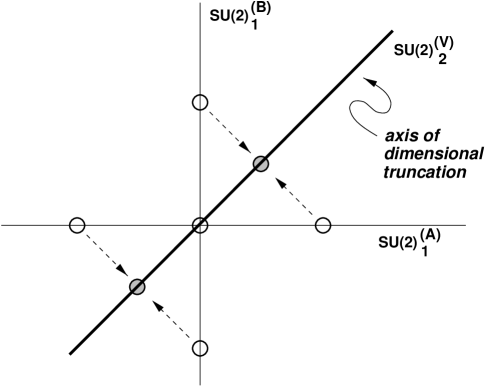
Figure 7: The root system of $SU(2)_{1}^{(A)}\times SU(2)_{1}^{(B)}$ (denoted by open circles), and its dimensional truncation onto the diagonal subgroup $SU(2)_{2}^{(V)}$ (with new non-zero roots denoted by shaded circles).

As an example of how such “dimensional truncations” work, let us consider the well-known method of achieving a level-two affine Lie algebra which consists of tensoring together two copies of any group $G$ at level one, and then modding out by the symmetry interchanging the two group factors. This leaves behind the diagonal subgroup $G$ at level two. This construction is well-known in the case $G=E_{8}$, where it serves as the underlying mechanism responsible for the non-supersymmetric (level-two) single-$E_{8}$ string model in ten dimensions [32]. For simplicity, let us analyze this construction for the case $G=SU(2)$. If we start with an $SU(2)_{1}^{(A)}\times SU(2)_{1}^{(B)}$ gauge symmetry, as illustrated in Fig. 7, then modding out by their interchange symmetry [i.e., constructing the diagonal subgroup $SU(2)^{(V)}$] corresponds to projecting or dimensionally truncating the roots onto the diagonal axis corresponding to the diagonal Cartan generator $J_{z}^{(V)}=J_{z}^{(A)}+J_{z}^{(B)}$. As we can see from Fig. 7, this reproduces the $SU(2)$ root system, but scaled so that roots which formerly had length $\sqrt{2}$ now have length $1$. Thus we have realized $SU(2)$ at level two as the diagonal survivor of this dimensional-truncation procedure. Indeed, it is clear that this diagram generalizes to any groups $G_{1}^{(A)}\times G_{1}^{(B)}$, since the roots of the two level-one root systems are always orthogonal to each other, and hence project onto the diagonal axes with a reduction in length by a factor $\cos\,45^{\circ}=1/\sqrt{2}$. Moreover, we see that this also generalizes to any number of identical group factors tensored together, $G_{1}^{(1)}\times G_{1}^{(2)}\times...G_{1}^{(n)}$, leaving behind the completely diagonal subgroup $G$ at level $n$. More sophisticated examples of such dimensional truncations, along with descriptions of their basic properties and uses, can be found in Ref. [7].

4.3 Current status and recent developments

Thus far we have described, in a model-independent way, the basic ingredients that go into the realization of higher-level gauge symmetries in string theory. However, the construction of an actual satisfactory string GUT model is a far more difficult affair. In particular, while the methods for realizing the special GSO projections that effect rank-cutting are now well-understood, it is still necessary to reconcile these special projections with the “ordinary” GSO projections that yield, for example, (1) three and only three massless chiral generations; (2) no extra exotic chiral matter; and (3) the proper Higgs content and couplings (e.g., in order to avoid proton decay). Indeed, in string GUT models (just as in ordinary field-theoretic GUT models), the problem of proton decay is a vital issue.

Until recently, it appeared that such a reconciliation might not be possible. In particular, despite various early attempts [20, 21], no three-generation models with higher-level GUT symmetries had been constructed, and it might have seemed that the requirement of three generations might, by itself, be in fundamental conflict with the requirement of higher-level gauge groups. However, it has recently been shown that this is not the case for a variety of GUT gauge groups and levels. A summary of those groups and levels for which consistent three-generation string GUT models have been constructed appears in Table 2. In particular, level-two $SU(5)$ models were obtained in Ref. [22] using a symmetric orbifold construction and in Ref. [23] using the free-fermionic construction [30, 31]. By contrast, level-three $SU(5)$, $SO(10)$, and $E_{6}$ models were obtained in Refs. [24, 25] using an asymmetric orbifold construction developed in Ref. [29]. All of these models realize their higher-level gauge symmetries via the diagonal embeddings discussed above, and contain extra matter (beyond the three massless generations and adjoint Higgs representations) in their massless spectra.

  $k=2$   $k=3$   $k=4$ $SU(5)$ $\surd$ $\surd\surd$ ? $SO(10)$ ? $\surd\surd$ ? $E_{6}$ ? $\surd\surd$ ?

Table 2: Progress in the construction of three-generation higher-level string GUT models. A single check ($\surd$) indicates the construction of three-generation string models with extra chiral matter in the massless spectrum, whereas a double check ($\surd\surd$) signifies the construction of three-generation string models with extra non-chiral (vector-like) matter in the massless spectrum. No three-generation models have been constructed without additional chiral or vector-like matter. Question marks indicate that no three-generation models have yet been constructed.

The existence of these three-generation models clearly demonstrates that such string GUT models are possible. Unfortunately, it is not yet clear whether such models are entirely “realistic”, for the other problems listed above tend to remain unresolved for the string GUT models. For example, the three-generation level-two $SU(5)$ models constructed in Refs. [22, 23] all contain extra chiral ${\bf{15}}$ representations of $SU(5)$, which would give rise to extra color sextets after GUT symmetry breaking. Indeed, because these states are chiral, they remain light and are thus phenomenologically unacceptable. Likewise, the three-generation level-three models, although promising, have yet to be examined in detail, and in particular it remains to examine their superpotentials and Higgs couplings to see if realistic low-energy phenomenologies are possible and if any undesirable extra vector-like matter can be made superheavy. However, the pace of recent progress in both the free-fermionic and orbifold constructions — along with the recent construction of three-generation higher-level string models — suggests that the problems faced in this approach are now simply those of constructing realistic models, and are not fundamental. Further advances in model construction are therefore likely.

There have also been recent developments in understanding general properties of such higher-level string GUT models. All of the above string models that have been constructed use the so-called “diagonal construction” in which the level-$k$ GUT gauge group $G$ is realized as the diagonal subgroup within a $k$-fold tensor-product of group $G$ at level one:

$$G_{k}~{}\subset~{}G~{}\times~{}G~{}\times~{}...~{}\times~{}G~{}.$$ (4.5)

Such diagonal embeddings were described in Sect. 4.2.2, and were illustrated in Fig. 7 for the case of $SU(2)_{2}$. Unfortunately, however, the diagonal construction is a very expensive and inefficient way of realizing such higher-level gauge groups, for it requires that one first build a string model with the larger gauge group $G\times G\times...\times G$, and then subsequently break to the diagonal subgroup. Indeed, because of its larger rank, this tensor-product group typically occupies many more dimensions of the charge lattice than would be required for only the higher-level subgroup; it also requires greater central charge than the higher-level subgroup itself would require. Thus, such diagonal realizations of higher-level gauge symmetries come with extra hidden “costs” beyond those due to the higher-level gauge symmetries themselves, and imply that such string models will have smaller hidden-sector gauge symmetries than would otherwise be possible. This in turn means that one has less flexibility for controlling or arranging many other desired phenomenological features of a given string model. It would therefore be useful to have a general method of surveying whether the diagonal embeddings in Eq. (4.5) are the only embeddings that can be employed for realizing higher-level GUT gauge symmetries in free-field string constructions, or whether other more efficient embeddings are possible.

$G^{\prime}_{k}$ $\subset$ $G$ $\Delta c$ $\Delta r$ $\xi$ $SU(5)_{2}$ Diagonal only $8/7$ 4 $SU(5)_{3}$ $SU(10)_{1}$ $0$ 5 $+3$ $SU(5)_{4}$ $SU(15)_{1}$ $10/3$ 10 $+2$ $SU(5)_{4}$ $SU(16)_{1}$ $13/3$ 11 $+1$ $SU(6)_{2}$ Diagonal only $5/4$ 5 $SU(6)_{3}$ Diagonal only $10/3$ 10 $SU(6)_{4}$ $SU(15)_{1}$ $0$ 9 $+6$ $SO(10)_{2}$ $SU(10)_{1}$ $0$ 4 $+1$ $SO(10)_{3}$ Diagonal only $30/11$ 10 $SO(10)_{4}$ $SU(16)_{1}$ $0$ 10 $+5$ $SO(10)_{4}$ $[SU(10)_{1}]^{2}$ $3$ 13 $+2$ $SO(10)_{4}$ $SU(10)_{1}\times[SO(10)_{1}]^{2}$ $4$ 14 $+1$ $SO(10)_{k>4}$ Impossible $(E_{6})_{2}$ Diagonal only $6/7$ 6 $(E_{6})_{3}$ Diagonal only $12/5$ 12 $(E_{6})_{k>3}$ Impossible

Table 3: The complete list of all possible non-diagonal free-field string embeddings that can give rise to $SU(5)_{k}$, $SU(6)_{k}$, $SO(10)_{k}$, and $(E_{6})_{k}$ at levels $2\leq k\leq 4$. Here $\Delta r$ and $\Delta c$ are the extra rank and central charge required for each embedding, and $\xi$ is the “savings” in these quantities relative to the corresponding diagonal embedding.

Such a general survey has recently been completed [7]. By studying the dimensional truncations that are necessary in order to achieve higher-level gauge symmetries, it has been shown [7] that each such truncation corresponds uniquely to a so-called “irregular” embedding in group theory. Given this information, it has now been possible to classify all possible ways of realizing higher-level gauge symmetries in free-field string theories [7], and a complete list of all embeddings for the GUT groups $SU(5)$, $SU(6)$, $SO(10)$, and $E_{6}$ for levels $k=2,3,4$ is given in Table 3. For each such embedding $G^{\prime}_{k}\subset G$, we have also listed the extra ranks and central charges that are required for its realization,

$$\Delta r = {\rm rank}\,G~{}-~{}{\rm rank}\,G^{\prime}$$

$$\Delta c = c(G)~{}-~{}c(G^{\prime}_{k})~{},$$ (4.6)

where the central charges are computed according to Eq. (4.1). Note that in many cases, the only possible higher-level embeddings are in fact the diagonal embeddings. However, it is evident from Table 3 that there also exist many new classes of embeddings which might form the basis for new types of string GUT model constructions. In particular, some of these new embeddings require less rank and central charge for their realization than the diagonal embeddings, and are therefore significantly more efficient. For such embeddings, we have defined the quantity $\xi$ which appears in Table 3 in such a way as to measure this improved efficiency in central charge and rank relative to the diagonal embedding:

$$\xi~{}\equiv~{}k~{}c(G^{\prime}_{1})~{}-~{}c(G)~{}=~{}k\,({\rm rank}\,G^{\prime})~{}-~{}{\rm rank}\,G~{}.$$ (4.7)

Thus, embeddings with $\xi>0$ are always more efficient than their diagonal counterparts.

This complete classification of higher-level GUT embeddings has also made it possible to obtain new restrictions on the possibilities for potentially viable string GUT models. Certain phenomenological characteristics of string GUT models are, of course, immediately obvious from Table 1 directly. For example, since the ${\bf 54}$ representation of $SO(10)$ at level two already saturates the $h_{R}=1$ masslessness constraint, this representation cannot carry any additional quantum numbers under any gauge symmetries beyond $SO(10)$ in such models. This in turn restricts its allowed couplings [22], essentially ruling out couplings of the forms $X\cdot{\bf 54}\cdot{\bf 54}$ or $X\cdot{\bf 54}\cdot{\bf 54^{\prime}}$ where $X$ is any chiral field which transforms as a singlet under $SO(10)$. Likewise, again following similar sorts of arguments, it has been shown [22] that all superpotential terms in string GUT models must have dimension $\geq 4$. In other words, explicit mass terms (which would have dimension two) are ruled out. Other phenomenological consequences of the results in Table 1, especially as they restrict the possibilities for hidden-sector phenomenology, can be found in Ref. [33]. Indeed, such string GUT “selection rules” are completely general, and apply to all string constructions.

However, given the recent classification of GUT embeddings in Table 3, it is now possible to go beyond these sorts of constraints in the case of string models using free-field constructions. For example, it has been shown in Ref. [7] that $SO(10)$ can never be realized at levels exceeding four in free-field string constructions; this result clearly goes beyond the simple central-charge constraint (which would have permitted realizations up to $k=7$), and thereby implies, for instance, that it is impossible to realize the useful 126 representation within such $SO(10)$ string GUT models. A more detailed study [34] shows, in fact, that in free-field heterotic $SO(10)$ string models using diagonal embeddings, all representations larger than the 16 must always transform as singlets under all gauge symmetries beyond $SO(10)$; moreover, such constructions can never give rise to the ${\bf 120}$ or ${\bf 144}$ representations of $SO(10)$. These results hold regardless of the affine level at which $SO(10)$ is realized (i.e., despite the general results of Table 1), and essentially reflect the additional costs that are involved when realizing higher-level gauge symmetries through diagonal embeddings in free-field string constructions [7, 34]. Indeed, the only known exception to these rules takes place in a phenomenologically unrealistic non-chiral string model (see, e.g., Appendix B of Ref. [25]). Likewise, a similar analysis [34] for $E_{6}$ shows that $E_{6}$ can never be realized beyond level three in free-field constructions (even though the central-charge constraint would have permitted level four); moreover, one finds that the adjoint ${\bf 78}$ representation must always transform as a singlet under all gauge symmetries beyond $E_{6}$. Taken together, then, these results thus severely limit the types of phenomenologically realistic field-theoretic $SO(10)$ and $E_{6}$ models that can be obtained using such string constructions. These issues are discussed more fully in Ref. [34].

Of course, there are various ways around these difficulties. One method is to employ the non-diagonal embeddings listed in Table 3; at present, these new embeddings have not been explored in the literature, but it has been shown that they may have improved phenomenological prospects [7, 34]. Another method is to adopt a string construction which is not based on free worldsheet fields. Such constructions include, for example, those based on tensor products of Wess-Zumino-Witten models [35], such as Gepner or Kazama-Suzuki models. These constructions are quite difficult to implement in practice, however, and thus have not been investigated for phenomenological purposes.

4.4 String GUT models without higher levels?

The complicated issues that arise when constructing higher-level string GUT models should not be taken to indicate that the GUT idea cannot be made to work in a simple manner in string theory. Indeed, even if no completely realistic higher-level string GUT models are ultimately constructed, there exists an entirely different approach which, although technically not a “string GUT”, is equally compelling. These are the so-called $G\times G$ models, which have been examined in both string-theoretic [21, 22, 36, 37] and field-theoretic [38] contexts. The basic idea is as follows. We have seen in Fig. 7 that one can realize a gauge symmetry group $G$ at level $k_{G}=2$ by starting with a gauge symmetry $G\times G$ realized at level one, and then modding out by the $\mathchoice{\hbox{\cmss Z\kern-3.99994ptZ}}{\hbox{\cmss Z\kern-3.99994ptZ}}{\lower 0.9pt\hbox{\cmsss Z\kern-2.79996ptZ}}{\lower 1.2pt\hbox{\cmsss Z\kern-2.79996ptZ}}_{2}$ symmetry that interchanges the two group factors. Indeed, this is just the diagonal construction. In the string GUT models that we have been discussing up to this point, this final step (the $\mathchoice{\hbox{\cmss Z\kern-3.99994ptZ}}{\hbox{\cmss Z\kern-3.99994ptZ}}{\lower 0.9pt\hbox{\cmsss Z\kern-2.79996ptZ}}{\lower 1.2pt\hbox{\cmsss Z\kern-2.79996ptZ}}_{2}$ modding) is done within the string construction itself, so that at the Planck scale, the string gauge symmetry group is $G$ at level $k=2$. However, an alternative possibility is simply to construct a string model with the level-one gauge symmetry $G\times G$, and then do the final breaking to the diagonal subgroup $G$ in the effective field theory at some lower scale below the Planck scale. It turns out that all that is required for this breaking is a Higgs in the fundamental representation of $G\times G$, and after the breaking one effectively obtains the adjoint Higgs required for further breaking to the MSSM gauge group:

$$SU(5): ({\bf{5}},\overline{{\bf{5}}})~{}\to~{}{\bf{24}}~{}+~{}{\bf{1}}~{}$$

$$SU(6): ({\bf{6}},\overline{{\bf{6}}})~{}\to~{}{\bf{35}}~{}+~{}{\bf{1}}~{}$$

$$SO(10): ({\bf{10}},{\bf{10}})~{}\to~{}{\bf{45}}~{}+~{}{\bf{54}}~{}+~{}{\bf{1}}~{}.$$ (4.8)

Thus, simply by utilizing the fundamental representations available at level one at the string scale, one can nevertheless produce effective adjoint representations at lower scales. String models utilizing this mechanism have been investigated by several authors [21, 22, 36, 37], and have met with roughly the same level of success as achieved in the level-two constructions. In particular, three-generation $G\times G$ string models have been constructed for the case of $G=SU(5)$, and in fact one such model [37] apparently contains no extra chiral matter in its massless spectrum. Note that while this mechanism works in principle for $SU(5)$, $SU(6)$, and $SO(10)$, it cannot be used for $E_{6}$ since the necessary initial representation $({\bf{27}},\overline{{\bf{27}}})$ would have $h>1$ and thus could not appear in the massless spectrum.

We see, then, that the $G\times G$ models clearly represent an alternative scenario which, although not a strict “string GUT”, could still resolve the gauge coupling unification problem in the GUT manner, with a unification of MSSM couplings at $M_{\rm MSSM}$, followed by the running of a single GUT coupling between $M_{\rm MSSM}$ and $M_{\rm string}$. An interesting fact which has recently been pointed out [39], however, is that such $G\times G$ models typically give rise to moduli which transform in the adjoint of the final gauge group $G$. As shown in Refs. [39, 40] for the case of color octet moduli and electroweak triplet moduli with vanishing hypercharge, such extra adjoint states have the potential to alter the running of the gauge couplings in such a way as to fix the original discrepancy between $M_{\rm MSSM}$ and $M_{\rm string}$ which motivated the consideration of the GUT in the first place. Of course, it is not known a priori whether these states will actually have the masses required to resolve this discrepancy. In any case, the phenomenological problems that afflict the higher-level string models using diagonal embeddings become even more severe for these level-one $G\times G$ models, and thus must still be addressed.

Finally, we mention that the subtleties with higher levels can also be avoided by employing a GUT scenario that does not require an adjoint Higgs for breaking to the MSSM gauge group. An example of such a GUT scenario is flipped $SU(5)$ [41], in which the required gauge symmetry is $G=SU(5)\times U(1)$ and the matter embedding within $G$ is “flipped” relative to that of ordinary $SU(5)$. Another example is the Pati-Salam unification scenario [42], for which $G=SO(6)\times SO(4)$. These field-theoretic unification scenarios have been realized within consistent three-generation string models [43, 44], and will be discussed at various points in Sects. 6–8. Furthermore, even within the level-one “strict GUT” scenarios, it may be possible to overcome the absence of adjoint Higgs representations by utilizing the string states with fractional electric charge that often appear in such string models [45, 46]. As recently suggested in Ref. [47], such states can in principle serve as “preons” which may bind together under the influence of hidden-sector gauge interactions in order to form effective adjoint Higgs representations. We shall discuss the appearance of fractionally charged string states in Sect. 5.4.

Thus, we see that although the string GUT approach to understanding gauge coupling unification is quite subtle and complicated, there has been substantial progress in recent years both in understanding the general properties of such theories as well as in the construction of realistic three-generation string GUT models.

5 Path #2: Unification via Non-Standard Levels $(k_{Y},k_{2},k_{3})$

The second possible path to string-scale unification preserves the MSSM gauge structure between the string scale and the $Z$ scale, and instead attempts to reconcile the discrepancy between the MSSM unification scale and the string scale by adjusting the values of the string affine levels $(k_{Y},k_{2},k_{3})$. The MSSM unification scale, of course, is determined under the assumption that $(k_{Y},k_{2},k_{3})$ have their usual MSSM values $(5/3,1,1)$ respectively. However, in string theory the possibility exists for the MSSM gauge structure to be realized with different values of $(k_{Y},k_{2},k_{3})$, thereby altering, as in Eq. (2.6), the predicted boundary conditions for gauge couplings at unification. The possibility of adjusting these parameters (especially $k_{Y}$) was first proposed in Ref. [48], and has been considered more recently in Refs. [49, 6, 23, 50].

5.1 What is $k_{Y}$?

Before discussing whether such realizations are possible, we first discuss the definition of $k_{Y}$. As we explained in Sect. 4, $k_{2}$ and $k_{3}$ are the affine levels of the $SU(2)$ and $SU(3)$ factors of the MSSM gauge group, and these levels are defined through the relation (2.7). The hypercharge group factor $U(1)_{Y}$, by contrast, is abelian, and thus there are no corresponding structure constants $f^{abc}$ or non-zero roots $\vec{\alpha}_{h}$ through which to fix the magnitudes of the terms in the hypercharge current-current OPE. In other words, there is no way in which a unique normalization for the hypercharge current $J_{Y}$ can be chosen, and consequently there is no intrinsic definition of $k_{Y}$ which follows uniquely from the algebra of hypercharge currents. Thus, the definition of $k_{Y}$ requires a convention.

In order to fix a convention, we examine something physical, namely scattering amplitudes. The following argument originates in Ref. [13], and details for the case of abelian groups can be found in Refs. [51, 6]. For a non-abelian group, the gauge bosons experience not only couplings to gravity (through vertices of the form $WWg$ where $W$ is a non-abelian gauge boson and $g$ is a graviton), but also trilinear self-couplings (through vertices of the form $WWW$). It then turns out that $k_{G}$ is essentially the ratio of these vertices. Indeed, the $WWg$ vertex factor is derived from the double pole term in Eq. (2.7), whereas the $WWW$ vertex factor is derived from the single pole term in Eq. (2.7). For an abelian group, however, we have only vertices of the form $YYg$. We nevertheless define a normalization $k_{Y}$ for the $U(1)_{Y}$ current $J_{Y}$ in such a way that it has the same coupling to gravity as a non-abelian current. As shown in Ref. [13], this is tantamount to requiring that $J_{Y}$ have a normalization giving rise to the OPE

$$J_{Y}(z)\,J_{Y}(w)~{}=~{}{1\over(z-w)^{2}}~{}+~{}{\rm regular}~{}.$$ (5.1)

Given this normalization, we then compute the ratio of the corresponding coupling $g_{Y}$ with the gravitational coupling, and find

$$8\pi\,{G_{N}\over\alpha^{\prime}}~{}=~{}2\,g_{Y}^{2}~{}.$$ (5.2)

Thus, in analogy with Eq. (2.6), we define $k_{Y}=2$ for an abelian current normalized according to Eq. (5.1).

Given these results, it is then straightforward to determine the value of $k_{Y}$ corresponding to any $U(1)$ current: we simply determine the coefficient of the double-pole term in the corresponding current-current OPE,

$$J_{Y}(z)\,J_{Y}(w)~{}=~{}{k_{Y}/2\over(z-w)^{2}}~{}+~{}{\rm regular}~{}.$$ (5.3)

Defining $k_{Y}$ in this way then insures that the tree-level coupling constant relation (2.6) holds for abelian group factors as well:

$$8\pi\,{G_{N}\over\alpha^{\prime}}~{}=~{}k_{Y}\,g_{Y}^{2}~{}.$$ (5.4)

Thus, in this manner, an invariant meaning can be given to the “affine level” $k_{Y}$ of any abelian group factor $U(1)_{Y}$.

In practice, in a given string model, the $U(1)$ hypercharge current $J_{Y}$ will typically be realized as a linear combination of the elementary $U(1)$ currents $J_{i}$ ($i=1,...,22$) which comprise the Cartan subalgebra of the gauge group of the model:

$$J_{Y}~{}=~{}\sum_{i}\,a_{i}\,J_{i}~{}.$$ (5.5)

Here $a_{i}$ are coefficients which represent the embedding of the hypercharge current $J_{Y}$ into the charge lattice of the model. Since each of these individual Cartan currents is normalized according to Eq. (5.1), we then find that

$$J_{Y}(z)\,J_{Y}(w)~{}=~{}{\sum_{i}{a_{i}}^{2}\over(z-w)^{2}}~{}+~{}{\rm regular}~{}.$$ (5.6)

Thus, for the current (5.5), we have

$$k_{Y}~{}=~{}2\,\sum_{i}\,{a_{i}}^{2}~{}.$$ (5.7)

The value of $k_{Y}$ is therefore completely determined by the particular hypercharge embedding $\{a_{i}\}$, and is a model-dependent quantity which depends on the way in which the hypercharge current is realized in a particular string construction.

5.2 Phenomenologically preferred values of $(k_{Y},k_{2},k_{3})$

Given these definitions of the levels for the abelian and non-abelian group factors, we must now determine the phenomenologically preferred values of $(k_{Y},k_{2},k_{3})$ which would reconcile string unification with the experimentally observed values [9] of the low-energy couplings given in Eq. (2.13).

The analysis is straightforward, and details can be found in Ref. [6]. We begin with the one-loop renormalization group equations (RGE’s) for the gauge couplings in the effective low-energy theory:

$${{16\pi^{2}}\over{g_{i}^{2}(M_{Z})}}~{}=~{}k_{i}\,{{16\pi^{2}}\over{g_{\rm string}^{2}}}~{}+~{}b_{i}\,\ln{M^{2}_{\rm string}\over{M_{Z}}^{2}}~{}+~{}\Delta_{i}^{\rm(total)}~{}.$$ (5.8)

Here $b_{i}$ are the one-loop beta-function coefficients, and we keep the affine levels $(k_{Y},k_{2},k_{3})$ arbitrary. In Eq. (5.8), the quantities $\Delta_{i}^{\rm(total)}$ represent the combined corrections from various string-theoretic and field-theoretic effects such as heavy string threshold corrections, light SUSY thresholds, intermediate gauge structure, and extra string-predicted matter beyond the MSSM. These corrections are all highly model-dependent, as they are strongly influenced by the particular string model or compactification under study. For the purposes of the present analysis, we shall ignore all of these corrections, for our goal in this section is to determine the extent to which a suitable foundation for string-scale gauge coupling unification can be established by choosing appropriate values for $(k_{Y},k_{2},k_{3})$, without resorting to large corrections from these other sources. (The effects of these other sources will be discussed in the following sections.) There are, however, some important corrections that are model-independent: these include the corrections that arise from two-loop effects, the effects of minimal Yukawa couplings, and the effects of renormalization-group scheme conversion (from the $\overline{\rm DR}$-scheme used in calculating $M_{\rm string}$ to the $\overline{\rm MS}$-scheme used in extracting the values of the low-energy gauge couplings from experiment). It turns out that these latter effects are quite sizable, and must be included.

Figure 8: Dependence of the unification scale $M_{\rm string}$ on the chosen value of $r\equiv k_{Y}/k_{2}$. The different curves correspond to different values of $\sin^{2}\theta_{W}(M_{Z})$ within its experimental limits, with the lower curve arising for greater values.

Figure 9: Parameter space of allowed values of $r^{\prime}\equiv k_{3}/k_{2}$ and $r\equiv k_{Y}/k_{2}$ that are consistent with the experimentally observed low-energy couplings. The different curves correspond to different values of the couplings within their experimental uncertainties, with the higher curves arising for smaller values of $\sin^{2}\theta_{W}(M_{Z})$ and $\alpha_{\rm strong}(M_{Z})$, and the lower curves arising for greater values. Different points on any single curve in this plot correspond to different unification scales.

Given the one-loop RGE’s (5.8), we then eliminate the direct dependence on the unknown string coupling $g_{\rm string}$ by solving these equations simultaneously in order to determine the dependence of the low-energy couplings on the affine levels $(k_{Y},k_{2},k_{3})$. If we define the ratios of the levels

$$r~{}\equiv~{}{k_{Y}\over k_{2}}~{}~{}~{}~{}~{}~{}~{}{\rm and}~{}~{}~{}~{}~{}~{}~{}r^{\prime}~{}\equiv~{}{k_{3}\over k_{2}}~{},$$ (5.9)

we then find that the low-energy couplings $\sin^{2}\theta_{W}$ and $\alpha_{\rm strong}$ at the $Z$ scale are given in terms of these ratios as

$$\sin^{2}\theta_{W}(M_{Z}) = {1\over{1+r}}\,\left[1~{}-~{}\left(b_{Y}-{r}\,b_{2}\right)\,{a\over 2\pi}\,\ln{M_{\rm string}\over M_{Z}}\right]~{}+~{}\Delta^{(\rm sin)}$$

$$\alpha_{\rm strong}^{-1}(M_{Z}) = {r^{\prime}\over 1+r}\,\left[{1\over a}~{}-~{}\left(b_{Y}+b_{2}-{1+r\over r^{\prime}}\,b_{3}\right)\,{1\over 2\pi}\,\,\ln{M_{\rm string}\over M_{Z}}\right]~{}+~{}\Delta^{(\alpha)}~{}.~{}~{}~{}~{}~{}~{}$$ (5.10)

Here $a\equiv\alpha_{\rm e.m.}(M_{Z})$ is the electromagnetic coupling at the $Z$ scale, and the correction terms in these equations are

$$\Delta^{\rm(sin)} = -\,{1\over 1+r}\,{a\over 4\pi}\,(\Delta_{Y}-r\,\Delta_{2})$$

$$\Delta^{(\alpha)} = -\,{r^{\prime}\over 1+r}\,{1\over 4\pi}\,\left(\Delta_{Y}+\Delta_{2}-{1+r\over r^{\prime}}\,\Delta_{3}\right)~{}$$ (5.11)

where $(\Delta_{Y},\Delta_{2},\Delta_{3})$ are the combined two-loop, Yukawa, and scheme-conversion corrections to the individual couplings $(g_{Y},g_{2},g_{3})$ in Eq. (5.8). It can be shown [6] that these corrections $\Delta_{Y,2,3}$ are approximately independent of the affine levels $k_{i}$. Thus, from Eqs. (5.10) and (5.11), we see that the magnitude of $\sin^{2}\theta_{W}$ depends on only the single ratio $r$, while the magnitude of $\alpha_{\rm strong}$ depends on only the single ratio $r^{\prime}/(1+r)$. These observations imply that the value of $k_{Y}/k_{2}$ can be determined purely by the value of the coupling $\sin^{2}\theta_{W}$ at the $Z$ scale, while the value of $k_{3}/k_{2}$ can then be adjusted in order to maintain an acceptable value for $\alpha_{\rm strong}$ at the $Z$ scale.

It is straightforward to evaluate these constraints on $(r,r^{\prime})$. For the MSSM with three generations and two Higgs representations, we have $(b_{Y},b_{2},b_{3})=(11,1,-3)$; we likewise take as fixed input parameters [52] the $Z$ mass $M_{Z}\equiv 91.161\pm 0.031$ GeV and the electromagnetic coupling at the $Z$-scale $a^{-1}\equiv\alpha_{\rm e.m.}(M_{Z})^{-1}=127.9\pm 0.1$. Given the experimentally measured low-energy couplings listed in Eq. (2.13) and the calculated values of the combined two-loop, Yukawa, and scheme-conversion corrections [6]

$$\Delta_{Y}~{}\approx~{}11.6~{},~{}~{}~{}~{}~{}~{}\Delta_{2}~{}\approx~{}13.0~{},~{}~{}~{}~{}~{}~{}\Delta_{3}~{}\approx~{}7.0~{},$$ (5.12)

we can now determine which values of $(r,r^{\prime})$ yield a successful unification. The results [6] are shown in Figs. 9 and 9. In Fig. 9, we show the dependence of the scale of unification on the choice of the ratio $r$; as expected, we find that $r=5/3$ leads to a unification scale approximately at $M_{\rm MSSM}\approx 2\times 10^{16}$ GeV, while unification at the desired string scale $M_{\rm string}\approx 5\times 10^{17}$ GeV occurs only for smaller values of $r$, typically $r\approx 1.5$. Note that this curve relies on only the low-energy input from $a\equiv\alpha_{\rm e.m.}(M_{Z})$ and $\sin^{2}\theta_{W}(M_{Z})$. In Fig. 9, by contrast, we see how the value of $r^{\prime}$ must then be correspondingly adjusted in order to maintain an experimentally acceptable value for $\alpha_{\rm strong}(M_{Z})$. Thus, Fig. 9 summarizes those combinations of $(r,r^{\prime})$ which are consistent with the phenomenologically acceptable values for each of the three low-energy couplings. It is clear from this figure that decreases in $r$ must generally be accompanied by increases in $r^{\prime}$ in order to obtain acceptable low-energy couplings; moreover, only the approximate region $1.5\leq r\leq 1.8$ is capable of yielding $r^{\prime}\approx 1$. This is an important constraint, for the non-abelian affine levels $k_{2}$ and $k_{3}$ are restricted to be integers, and thus arbitrary non-integer values of $r^{\prime}$ could generally be approximated only with extremely high levels $k_{2},k_{3}\gg 1$.

The analysis thus far has only constrained the values of the ratios of the levels $(k_{Y},k_{2},k_{3})$, for the renormalization group equations (5.10) give us no constraints concerning the absolute sizes of the affine levels. Fortunately, however, there is one additional constraint which must be imposed in order to reflect the intrinsically stringy nature of the unification. In field theory, there are ordinarily two independent parameters associated with unification: the value of the coupling at the unification scale, and the unification scale itself. In string theory, by contrast, these two parameters are tied together via Eq. (2.10). Thus, in string theory it is actually not sufficient to determine the ratios $k_{Y}/k_{2}$ and $k_{3}/k_{2}$ by merely demanding that they agree with low-energy data. Rather, we must also demand that if our low-energy couplings are run up to the unification point in a manner corresponding to certain values of the levels $(k_{Y},k_{2},k_{3})$, then the value of the predicted coupling $g_{\rm string}$ at the unification scale must be in agreement with that unification scale. If this final constraint is not met, we have not achieved a truly “stringy” unification.

This constraint may be imposed as follows [6]. We can choose one of our three couplings at low energy (the electromagnetic coupling, for example), and allow it to run upwards in energy until its value as a function of the mass scale coincides with the mass scale itself as in Eq. (2.10). This then yields the following transcendental self-consistency equation [6] which constrains the allowed values of the coupling (or equivalently, the unification scale) as a function of the affine levels that govern the running:

$${1\over\alpha_{\rm str}}~{}=~{}{1\over k_{Y}+k_{2}}\,\left[{1\over a}~{}-~{}{b_{Y}+b_{2}\over 2\pi}\,\ln\,{\sqrt{4\pi\alpha_{\rm str}}\,(5.27\times 10^{17}\,{\rm GeV})\over M_{Z}\,({\rm GeV})}\right]~{}+~{}\Delta^{(\rm trans)}~{}.~{}~{}~{}~{}~{}$$ (5.13)

Here $\alpha_{\rm str}\equiv g_{\rm string}^{2}/(4\pi)$, and the combined two-loop, Yukawa, and scheme-conversion correction $\Delta^{(\rm trans)}$ is given in terms of the individual corresponding $\Delta_{i}$ in Eq. (5.8) by

$$\Delta^{(\rm trans)}~{}=~{}-\,{\Delta_{Y}+\Delta_{2}\over k_{Y}+k_{2}}~{}.$$ (5.14)

The important thing to notice about this self-consistency constraint is that it depends on the absolute values of the affine levels, and not only on their ratios. Thus, by combining this constraint with our previous experimental constraints, we can fix not only the ratios $k_{Y}/k_{2}$ and $k_{3}/k_{2}$ of the affine levels, but also their absolute values.

Figure 10: Numerical solutions to the transcendental equation (5.13) for different values of $k_{Y}+k_{2}$, with the two-loop, Yukawa, and scheme-conversion corrections included (upper curve), and omitted (lower curve).

Figure 11: Dependence of $k_{2}$ on $r\equiv k_{Y}/k_{2}$. In this plot, the different curves correspond to different values of $\sin^{2}\theta_{W}(M_{Z})$, with the lower/left curves arising for greater values.

These final results are shown in Figs. 11 and 11. In Fig. 11, we display the numerical solutions to the transcendental self-consistency equation (5.13), plotting $g_{\rm string}\equiv\sqrt{4\pi\alpha_{\rm str}}$ as a function of $k_{Y}+k_{2}$, both with and without the two-loop, Yukawa, and scheme-conversion corrections. As we can see, the effect of the corrections (5.14) is quite significant. For $k_{Y}+k_{2}=5/3+1=8/3$, we find, as expected, that $0.7\leq g_{\rm string}\leq 1.0$, while for higher values of $k_{Y}+k_{2}$, the required string coupling increases significantly. Finally, combining this result with Fig. 9, we obtain Fig. 11: this strong dependence between $r\equiv k_{Y}/k_{2}$ and $k_{2}$ arises because the choice of a particular value of $r\equiv k_{Y}/k_{2}$ not only sets a particular unification scale, but with that choice of scale comes a certain scale for the string coupling via Eq. (2.11), and this in turn requires, via Eq. (5.13), a certain absolute magnitude for the affine levels. This combined dependence is clearly quite dramatic. In particular, we see from this figure that values of $r$ in the range $1.45\leq r\leq 1.5$ are consistent with relatively small affine levels $k_{2,3}=1,2$, but that for smaller values of $r$, the required affine levels increase dramatically. Of course, the precise placement of the curves in this plot depends quite strongly on the exact value of $\sin^{2}\theta_{W}(M_{Z})$ (as shown), as well as on the various threshold corrections we have been neglecting. Indeed, although we expect these curves to remain essentially independent of these corrections above $r\approx 1.45$, we see that the region $r<1.45$ depends exponentially on the precise corrections. Thus, the lower-$r$ regions of these curves are best interpreted as qualitative only. Nevertheless, the general shapes of these curves, evidently requiring extremely large changes in the absolute values of $k_{2}$ and $k_{3}$ for seemingly modest shifts in the ratio $r\equiv k_{Y}/k_{2}$, are striking and should provide extremely strong constraints on realistic string model-building.

It is clear, then, that only certain tightly-constrained values $(k_{Y},k_{2},k_{3})$ are phenomenologically allowed if we are to achieve string-scale unification with only the MSSM spectrum, and without resorting to large corrections from heavy string thresholds or extra non-MSSM matter. Indeed, from Figs. 9 and 11, we see that the best phenomenologically allowed regions of $(k_{Y},k_{2},k_{3})$ exist in a narrow band stretching through different values of $r$ in the range $1.4\leq r\leq 1.5$. For example, at the lower end of this band ($r\approx 1.4$) we have values such as $(k_{Y},k_{2},k_{3})\approx(21,15,17)$, whereas at intermediate regions of the band ($r\approx 1.42$) we have values such as $(k_{Y},k_{2},k_{3})\approx(14.2,10,11)$, and at higher regions ($r\approx 1.5$) we have $(k_{Y},k_{2},k_{3})\approx(1.5,1,1)$ or $(3,2,2)$.

Of course, strictly speaking, the smaller values of $r\approx 1.4$ are phenomenologically preferred, since they require the larger absolute values of $(k_{2},k_{3})$ which in turn enable us to more precisely approximate the required corresponding values of $r^{\prime}$ shown in Fig. 9. However, for the purposes of string model-building, it turns out that smaller values for the non-abelian affine levels, such as $k_{2},k_{3}=1~{}{\rm or}~{}2$, are strongly preferred on practical grounds. Indeed, not only does it grow increasingly difficult to build string models with higher values of $(k_{2},k_{3})$, but unwanted $SU(3)$ and $SU(2)$ representations of increasing dimensionality begin to appear in the massless spectrum as these non-abelian levels are increased. We have seen both of these features in Sect. 4. Thus, for the purposes of string model-building, the preferred regions of parameter space are actually in the higher-$r$ region, with $r\approx 1.5$ and with $k_{2}=k_{3}=1$ or $2$. One would then hope that relatively small corrections from other sources such heavy string thresholds would increase the effective value of $r^{\prime}$ from $r^{\prime}=1$ to $r^{\prime}\approx 1.05-1.1$. Furthermore, in this higher-$r$ region, such corrections are not expected to have a major effect on the validity of the curves in Fig 11.

Thus, in this “path to unification”, one attempts to realize string models or embeddings with affine levels in the range

$${\rm preferred~{}values}:~{}~{}~{}~{}~{}~{}~{}\cases{k_{2}~{}=~{}k_{3}~{}=~{}1~{}~{}{\rm or}~{}~{}2&{}\cr r~{}\equiv~{}k_{Y}/k_{2}~{}\approx~{}1.45-1.5~{}&~{}.\cr}$$ (5.15)

5.3 Hypercharge embeddings with $k_{Y}/k_{2}<5/3$ ?

Given the preferred affine levels in Eq. (5.15), the next question is to ask whether such levels (or combinations of levels) can be realized in string theory. What are the constraints that govern which combinations of $(k_{Y},k_{2},k_{3})$ are mutually realizable in self-consistent realistic string models?

Certain constraints are rather simple to formulate. For example, as we have already mentioned, worldsheet symmetries alone (namely, unitarity of the worldsheet conformal field theory) dictate that for non-abelian groups $G$, the corresponding affine levels $k_{G}$ are restricted to be integers. Thus $k_{2},k_{3}\in\mathchoice{\hbox{\cmss Z\kern-3.99994ptZ}}{\hbox{\cmss Z\kern-3.99994ptZ}}{\lower 0.9pt\hbox{\cmsss Z\kern-2.79996ptZ}}{\lower 1.2pt\hbox{\cmsss Z\kern-2.79996ptZ}}$. By contrast, $k_{Y}$ is the normalization of the abelian group factor $U(1)_{Y}$, and thus the value of $k_{Y}$ is arbitrary (as far as the worldsheet theory is concerned). Nevertheless, there are also spacetime phenomenological constraints that also come into play. For example, it is straightforward to show [46] that any phenomenologically consistent string model containing the MSSM right-handed electron singlet state $e_{R}$ must have $k_{Y}\geq 1$. This constraint essentially arises because the right-handed electron is a color- and electroweak-singlet in the MSSM. This implies that the sole contribution to the conformal dimension of this state from the Standard Model gauge group factors is solely that from its weak hypercharge $Y_{e_{R}}$. This state must also be massless, however. From Eq. (4.3), we then find

$${{\left(Y_{e_{R}}\right)}^{2}\over k_{Y}}~{}\leq~{}1~{},$$ (5.16)

and since $Y_{e_{R}}=1$ in the appropriate normalizations, we find $k_{Y}\geq 1$. Indeed, given all of the MSSM representations, it turns out that this is the strongest constraint that can be obtained in this manner.

The question then arises as to whether other phenomenological constraints can also be imposed on the value of $k_{Y}$. A general expectation might be that $k_{Y}=5/3$ is the minimal value allowed, simply because the standard $SO(10)$ embedding is an extremely economical way to embed all three generations with universal weak hypercharge assignment. Indeed, all of the realistic level-one string models constructed to date have $k_{Y}\geq 5/3$, and most trivial extensions of the $SO(10)$ embedding tend to increase the value of $k_{Y}$. Indeed, various initial searches for string models realizing $k_{Y}<5/3$ had been unsuccessful [49]. However, the possibility remains that there might exist special, isolated string models or constructions which manage to circumvent this bound, and populate the range $1\leq k_{Y}<5/3$. Thus, it is an important question to determine what values of $k_{Y}$ are allowed in string theory, and to determine whether the desired values $k_{Y}\leq 5/3$ (or, more generally, $k_{Y}/k_{2}\leq 5/3$) are even possible.

As we discussed at the beginning of this section, the “level” $k_{Y}$ corresponding to any abelian group factor is defined through the relation (5.3). Given a particular hypercharge embedding as in Eq. (5.5), the value of $k_{Y}$ is determined by Eq. (5.7). Of course, the particular hypercharge embedding that arises in a given string model is fixed in turn by the embeddings of the corresponding MSSM representations. Specifically, as we discussed in Sect. 4, corresponding to each MSSM state $s\in\{Q_{L},u_{R},d_{R},L_{L},e_{R},H^{+},H^{-}\}$ there exists a charge vector ${\bf Q}^{(s)}$, and we must carefully choose the coefficients $a_{i}$ in such a way that the quantity $\sum_{i}a_{i}Q_{i}^{(s)}$ reproduces the correct MSSM hypercharge assignment $Y^{(s)}$ for each state. This is a strong constraint, and it is not always possible to find such solutions in a given string model.

As a first step, therefore, we seek to determine whether there exist consistent MSSM embeddings that permit hypercharge solutions with $k_{Y}<5/3$. If so, we then seek to know whether such embeddings can be realized in consistent and realistic string models.

5.3.1 “Minimal” hypercharge embeddings

We first concentrate on recent results concerning the so-called “minimal” embeddings, since most realistic string models constructed to date employ such embeddings. By a “minimal” embedding, we refer to a hypercharge embedding in which the coefficients $a_{i}$ vanish for all of the lattice directions except those corresponding to the non-abelian MSSM gauge group factors $SU(3)_{C}\times SU(2)_{W}$. In most standard level-one string constructions, the color $SU(3)_{C}$ group factor is embedded within the first three lattice components ($i=1,2,3$), and the electroweak $SU(2)_{W}$ group factor is embedded within the next two components ($i=4,5$). Thus, in such cases, minimal hypercharge embeddings are those for which $a_{i}=0$ for $i\geq 6$.

Due to their tightly constrained nature, such minimal embeddings are particularly straightforward to analyze, and one can systematically attempt to construct MSSM embeddings (i.e., charge vectors ${\bf Q}$ for each of the MSSM representations plus Higgs representations) in such a way that they permit a consistent hypercharge assignment with $k_{Y}<5/3$. Of course, these MSSM embeddings are subject to a variety of constraints [6]. First, each MSSM charge vector must have the correct form corresponding to its representation under $SU(3)_{C}\times SU(2)_{L}$. Second, the length of each such charge vector is constrained by the appropriate masslessness condition. Third, each representation must have a charge vector which allows it to be realized as a chiral state; indeed, some charge vectors can be shown to correspond to non-chiral states only, with their chiral conjugates always present in the model. Another potential constraint that one may choose to impose is that these MSSM charge vectors should be consistent with having the required mass terms arise at the cubic level of the superpotential. Finally, one may also impose a moding constraint on the charge vectors; such a constraint generally reflects a particular set of allowed boundary conditions in a fermionic string construction, or equivalently a certain $\mathchoice{\hbox{\cmss Z\kern-3.99994ptZ}}{\hbox{\cmss Z\kern-3.99994ptZ}}{\lower 0.9pt\hbox{\cmsss Z\kern-2.79996ptZ}}{\lower 1.2pt\hbox{\cmsss Z\kern-2.79996ptZ}}_{N}$ twist in a bosonic formulation.

By analyzing all possible minimal embeddings, various results have recently been obtained. First, it has been shown that for a large class of realistic string models, one must always have [6]

$$k_{Y}~{}=~{}5/3\,,~{}11/3\,,~{}{\rm or}~{}14/3~{}.$$ (5.17)

This class includes all level-one string models with minimal embeddings in which the MSSM matter arises in sectors with $\mathchoice{\hbox{\cmss Z\kern-3.99994ptZ}}{\hbox{\cmss Z\kern-3.99994ptZ}}{\lower 0.9pt\hbox{\cmsss Z\kern-2.79996ptZ}}{\lower 1.2pt\hbox{\cmsss Z\kern-2.79996ptZ}}/2$ modings. Thus, for such models, we must always have $k_{Y}\geq 5/3$.

By contrast, it has also been shown that it is possible to circumvent this result by considering minimal embeddings beyond this class (i.e., embeddings with higher affine levels for the non-abelian MSSM group factors and/or higher modings for the MSSM matter). Indeed, although almost all of the consistent hypercharge embeddings beyond this class have $k_{Y}/k_{2}\geq 5/3$, it has been found [6] that there do exist several isolated embeddings which have $k_{Y}<5/3$. For example, given the level-one $SU(3)_{C}\times SU(2)_{L}$ embedding which is typically employed in the so-called “NAHE” models [53], the following MSSM matter embedding

$$Q_{L}:~{}~{} ~{}~{}~{}~{}~{}{\bf Q}=(-1/2,-1/2,1/2,0,1)$$

$$u_{R}:~{}~{} ~{}~{}~{}~{}~{}{\bf Q}=(1/4,1/4,-3/4,-3/4,-3/4)$$

$$d_{R}:~{}~{} ~{}~{}~{}~{}~{}{\bf Q}=(3/4,3/4,-1/4,-1/4,-1/4)$$

$$L_{L}:~{}~{} ~{}~{}~{}~{}~{}{\bf Q}=(-1/4,-1/4,-1/4,-3/4,1/4)$$

$$e_{R}:~{}~{} ~{}~{}~{}~{}~{}{\bf Q}=(1/2,1/2,1/2,1/2,1/2)$$

$$H^{+}:~{}~{} ~{}~{}~{}~{}~{}{\bf Q}=(1/4,1/4,1/4,3/4,-1/4)$$

$$H^{-}:~{}~{} ~{}~{}~{}~{}~{}{\bf Q}=(-1/4,-1/4,-1/4,-3/4,1/4)~{}$$ (5.18)

has a consistent hypercharge solution

$$Y~{}=~{}{5\over 12}\,(Q_{1}+Q_{2}+Q_{3})~{}+~{}{3\over 8}\,(Q_{4}+Q_{5})~{}.$$ (5.19)

This embedding, which satisfies all of the above-mentioned constraints including the cubic-level mass-term constraint, corresponds to $k_{Y}=77/48$, which is less than $5/3$. Clearly, this embedding makes use of $\mathchoice{\hbox{\cmss Z\kern-3.99994ptZ}}{\hbox{\cmss Z\kern-3.99994ptZ}}{\lower 0.9pt\hbox{\cmsss Z\kern-2.79996ptZ}}{\lower 1.2pt\hbox{\cmsss Z\kern-2.79996ptZ}}/4$ modings. Likewise, there also exist $k_{Y}/k_{2}<5/3$ embeddings which rely on having $k_{2}>1$ [6]. Unfortunately, it is not yet known whether such embeddings can be realized in actual string models. Thus, it is not known whether such embeddings are consistent with other desirable phenomenological properties such as $N=1$ spacetime SUSY, three and only three chiral generations, anomaly cancellation, and no unacceptable exotic matter.

5.3.2 “Extended” hypercharge embeddings

An alternative recent approach is to examine the so-called “extended” hypercharge embeddings [54, 23] in which the hypercharge current involves Cartan generators beyond those employed in realizing the non-abelian MSSM group factors. Because the structure of such embeddings is significantly less constrained than those of the minimal embeddings, they cannot be analyzed in a similar constructive manner. Nevertheless, by adequately sampling the space of string models (e.g., by computer), it is possible to find models that employ such extended hypercharge embeddings [23]. Moreover, it has recently been found that some of these models exhibit hypercharge embeddings with $k_{Y}<5/3$ along with $N=1$ spacetime SUSY, three complete chiral generations, and $U(1)$ anomaly cancellation. This, then, confirms the existence of string models with $k_{Y}<5/3$. In fact, several of these models also exhibit continuously variable values of $k_{Y}$; this surprising flexibility results from the freedom to continuously deform the particle identification in these models, ultimately providing a one-parameter family of possible charge assignments and corresponding values of $k_{Y}$ within a single model. Unfortunately, all of these models turn out to contain fractionally charged states that could survive in their light spectra. Whether such states may be removed without destroying these features or increasing $k_{Y}$ remains an open question.

5.4 Avoiding fractionally charged states

The appearance of color-neutral string states carrying fractional electric charge is a well-known problem in string theory [45], and is one of the problems that must be faced in any attempt to build a realistic string model. Such states represent a problem because of the strong constraints that stem from the failure of numerous experimental searches for such fractionally charged particles [55]. Unfortunately, the problem of color-neutral fractionally charged states in string theory becomes even more severe when attempting to build string models with non-standard values of $(k_{Y},k_{2},k_{3})$, for there exists a deep relation [46] between the values of these levels and the types of fractionally charged states that can appear in the corresponding string model. We shall now discuss this relation and some recent developments concerning its implications for gauge coupling unification.

The basic idea behind this relation can be found in Ref. [46], which in turn rests upon ideas developed in Refs. [56, 57]. Let us begin by supposing that our string model is based upon a rational worldsheet conformal field theory, and is to contain only those states which (after forming color-neutral bound states) carry integer electric charge. Given this requirement, it is possible to construct a certain current $\hat{J}$ in the worldsheet conformal field theory which satisfies two properties. First, $\hat{J}$ must be a simple current, meaning that it must have a one-term fusion rule with all other primary fields $\phi$ in the theory:

$$\hat{J}~{}\times~{}\phi~{}=~{}\phi^{\prime}~{}.$$ (5.20)

Second, $\hat{J}$ must be local with respect to all other primary fields $\phi$ which appear in the theory, so that the $\hat{J}\phi$ OPE takes the form

$$\hat{J}(z)\phi(w)~{}\sim~{}{\phi^{\prime}(w)\over(z-w)^{\alpha}}~{}+~{}...~{}$$ (5.21)

where the exponent $\alpha\equiv h(\hat{J})+h(\phi)-h(\phi^{\prime})$ is always an integer. Since this exponent can ultimately be related to the electric charge of the state created by $\phi$, it is the assumption of charge integrality for all of the string states which allows us to construct a current $\hat{J}$ for which Eq. (5.21) is always satisfied. Given any current $\hat{J}$ meeting these two conditions, it can then be shown that such a current must be a field which is also present in the theory. However, if this current is to be present in the theory, modular invariance then requires that its conformal dimension be an integer. Since the conformal dimension of $\hat{J}$ depends on the affine levels $(k_{Y},k_{2},k_{3})$, we thereby obtain a constraint on these levels. In other words, we thereby determine which combinations of affine levels are consistent with modular invariance and integrally charged states.

The result one finds [46] by carrying out this procedure is relatively simple: string models can be modular invariant and free of color-neutral fractionally charged states if and only if

$${k_{3}\over 3}~{}+~{}{k_{2}\over 4}~{}+~{}{k_{Y}\over 4}~{}\equiv~{}0~{}~{}~{}~{}~{}~{}({\rm mod}~{}1)~{}.$$ (5.22)

It is easy to see, then, that for $k_{2}=k_{3}=1$, the minimum allowed value of $k_{Y}$ is indeed $k_{Y}=5/3$. Thus, for level-one string models with only integer-charged states, we have

$$k_{Y}~{}\geq~{}5/3~{}.$$ (5.23)

We also obtain the same result for level-two models. Recall from Eq. (5.15) that gauge coupling unification requires $k_{2}=k_{3}$. Taking $k_{2}=k_{3}=2$ in Eq. (5.22) shows that $k_{Y}\geq 10/3$, so that once again $k_{Y}/k_{2}\geq 5/3$.

In general, though, string models do contain color-neutral fractionally charged states. In fact, as also shown in Ref. [46], it is impossible to have a level-one $SU(3)\times SU(2)\times U(1)_{Y}$ string model with $k_{Y}=5/3$ without having such fractionally charged states in the corresponding spectrum, for any GSO projections that would remove all of the fractionally charged states in such cases would also simultaneously promote the $SU(3)\times SU(2)\times U(1)_{Y}$ gauge symmetry to level-one $SU(5)$. How then can we reconcile our desire to have string models with $k_{Y}<5/3$ while simultaneously avoiding fractionally charged states?

One possibility is that such states can appear provided that they are confined under the influence of an additional confining “hypercolor” gauge interaction coming from a hidden sector beyond the MSSM. Indeed, heterotic string models typically have large (rank $\leq 18$) hidden-sector gauge groups $G$, and thus it is conceivable that although fractionally charged states may appear if $k_{Y}<5/3$, such states may fall into the particular representations of $G$ that permit them to be confined by $G$ into bound states with integral electric charge. However, it is first necessary to generalize the condition (5.22) to such cases, and to determine if there actually exist such confining scenarios which permit solutions with $k_{Y}\leq 5/3$. While various generalizations of Eq. (5.22) have been obtained [33, 58] for the specific binding scenarios and hypercolor groups available in certain string models with $k_{Y}\geq 5/3$, we here require a more general analysis which is capable of surveying all values of $k_{Y}$ and all possible binding groups $G$.

Such an analysis has recently been performed [6], and the results are as follows. For $k_{2}=k_{3}=1$, it is found that there are only sixteen possible choices of simple hypercolor groups $G$ and corresponding values of $k_{Y}<5/3$ for which all fractionally charged states can potentially be confined. Those with values of $k_{Y}$ in the phenomenologically interesting range $1.4\leq k_{Y}\leq 1.5$ are as follows:

    $$G$$    

(5.24)

The subscript on the hypercolor group $G$ indicates its level. For $k_{2}=k_{3}=2$, by contrast, there are more solutions. Those permitting values of $k_{Y}$ in the range $1.4\leq k_{Y}/k_{2}\leq 1.5$ are listed below:

    $$G$$              

17/12 17/12

3/2 73/51

13/9 17/12

22/15 17/12

49/33

(5.25)

Thus, for $k_{2}=k_{3}=2$, we see that relatively small hypercolor groups can now confine the fractionally charged states that arise for $1.4\leq k_{Y}/k_{2}\leq 1.5$. In particular, $SU(4)_{3}$, $SU(6)_{5}$, and $SU(9)_{1}$ are the most likely candidates for realization in consistent higher-level string models.

There are also other possible ways of avoiding fractionally charged states. Since the charge-integrality constraints we have discussed apply to all string states, such constraints might be evaded if we require that only the massless states be integrally charged. Another possibility would be to impose the even weaker requirement that only those massless states which are chiral must be integrally charged; after all, vector-like states which are fractionally charged and massless at tree level can acquire potentially large masses at higher loops (e.g., via the shift of the moduli which is generally required in order to break pseudo-anomalous $U(1)$ gauge symmetries and restore spacetime supersymmetry [59]). Indeed, such vacuum shifts along flat directions have the potential to make various fractionally charged states superheavy [60, 61], and the mechanism by which this occurs will be discussed in more detail in Sect. 8.2. Such scenarios, however, are highly model-dependent, and thus cannot be readily incorporated into this sort of general analysis. They therefore must be analyzed in a model-by-model fashion.

6 Path #3: Heavy String Threshold Corrections

We now turn to the paths that involve adding “correction terms” to the MSSM RGE’s. These corrections include those that arise from heavy string thresholds, light SUSY thresholds, possible intermediate-scale gauge structure, and possible intermediate-scale matter beyond the MSSM. In all of these scenarios, therefore, we essentially preserve the MSSM gauge structure with the standard MSSM levels $(k_{Y},k_{2},k_{3})=(5/3,1,1)$, and instead seek to determine whether the correction terms $\Delta_{i}$ that such effects generate can be sufficient to resolve the discrepancy between the naive MSSM unification scale and the unification scale expected within string theory. These correction terms $\Delta_{i}$ influence the running of the gauge couplings as indicated in Eq. (5.8). In this section we shall concentrate on the corrections that arise from the heavy string thresholds, and defer our discussion of the remaining correction terms to Sects. 7 and 8.

6.1 Calculating heavy string threshold corrections

The so-called “heavy string threshold corrections” are the one-loop corrections from the infinite towers of massive string states that are otherwise ignored in studies of the low-energy spectrum. Thus, these corrections represent a purely “stringy” effect. Although these states have Planck-scale masses, there are infinitely many of them, and thus the combined contributions $\tilde{\Delta}_{i}$ from such heavy string modes have the potential to be quite sizable. Since these corrections depend on the precise distributions of states at all mass levels of the string, they depend crucially on the particular choice of string vacuum. Thus, these corrections are generally moduli-dependent.

In general, for a given string vacuum and gauge group $G$, the corresponding threshold corrections $\tilde{\Delta}_{G}$ are determined to one-loop order by calculating the one-loop renormalization of the gauge couplings in the presence of a background gauge field. The threshold correction $\tilde{\Delta}_{G}$ is then deduced by comparing the coefficients of the gauge field-strength terms ${1\over 4}F^{a}_{\mu\nu}F_{a}^{\mu\nu}$ in the bare and one-loop effective Lagrangians. As illustrated in Fig. 12, this renormalization calculation is essentially analogous to the standard field-theoretic one-loop vacuum polarization calculation, except that in string theory the full calculation involves evaluating the two-dimensional (worldsheet) correlation function $\langle F^{a}_{\mu\nu}F_{a}^{\mu\nu}\rangle$ on the torus. This procedure generalizes the field-theoretic vacuum polarization calculation in such a way that the full gravitational back-reactions of string theory are automatically incorporated.

Figure 12: Calculation of the running of gauge couplings in field theory and string theory. In field theory, the background-field method involves evaluating the one-loop vacuum polarization diagram shown at left. In string theory, this polarization diagram generalizes to become the torus diagram shown at right. However, the complete calculation in string theory (including gravitational back-reactions) requires the calculation of the full correlation function $\langle F^{a}_{\mu\nu}F_{a}^{\mu\nu}\rangle$ evaluated on the torus in the presence of a suitable regulator.

This calculation was originally performed by considering a string propagating in a non-trivial gauge-field background that obeys the classical string equations of motion and thereby preserves worldsheet conformal invariance [19]; an alternative approach uses the background-field method in which the gauge field is treated as a classical background in which the string propagates, and is quantized accordingly [62]. Both calculations yield similar results, however, and it is found that $\tilde{\Delta}_{G}$ splits into two pieces of the form

$$\tilde{\Delta}_{G}~{}=~{}k_{G}\,Y~{}+~{}\Delta_{G}~{}.$$ (6.1)

Here $k_{G}$ is the affine level of the gauge group $G$; $Y$ is a certain quantity [63, 64, 65, 66] which is independent of the gauge group in question; and the remaining term $\Delta_{G}$ has a highly non-trivial dependence on the gauge group. In general, $Y$ receives the contributions arising from gravitational back-reactions of background gauge fields and universal oscillator excitations (and is expected to be relatively small [64]), while $\Delta_{G}$ receives contributions from massive compactification modes. Indeed, as we shall see, $\Delta_{G}$ simply tallies the contributions of all of the massive string states as they propagate around the one-loop torus diagram, and thus represents the generalization of the field-theoretic diagram as illustrated in Fig. 12. The importance of such contributions to the running of the effective low-energy couplings was pointed out early on (for example, in Ref. [67]), even before the formalism for calculating these string corrections was developed.

The decomposition in Eq. (6.1) is particularly useful because the term $k_{G}Y$ can simply be absorbed into a redefinition of the string coupling at unification:

$${1\over g_{\rm string}^{2}}~{}\to~{}{1\over g_{\rm string}^{2}}+{Y\over 16\pi^{2}}~{}.$$ (6.2)

This is convenient, for a proper calculation of $Y$ is fairly complicated and depends on having a suitable prescription for handling infrared divergences in string theory. We shall discuss this issue in Sect. 6.2. Moreover, for phenomenological purposes, we are often interested in only the relative running of the gauge couplings between different gauge group factors. If these different gauge groups are realized with equal affine levels, then the relative thresholds $\tilde{\Delta}_{G}-\tilde{\Delta}_{G^{\prime}}$ will be independent of $Y$. Recall from Eq. (5.15), for example, that equal affine levels are precisely what are required for the non-abelian group factors of the MSSM in order to achieve unification. We shall therefore defer a discussion of $Y$ to Sect. 6.2, and instead focus on the remaining term $\Delta_{G}$ in Eq. (6.1), which is found (in the $\overline{\rm DR}$ renormalization group scheme) to be given by [19]:

$$\Delta_{G}~{}\equiv~{}\int_{\cal F}{d^{2}\tau\over({\rm Im}\,\tau)^{2}}\,\biggl{[}B_{G}(\tau)~{}-~{}({\rm Im}\,\tau)\,b_{G}\biggr{]}~{}.$$ (6.3)

Here $b_{G}$ is the one-loop beta-function coefficient for the group $G$ (as determined in the effective theory by considering only the massless modes of the string), and $\tau$ is the toroidal complex modular parameter whose integration over the modular group fundamental domain ${\cal F}$ represents the summation over all conformally-inequivalent toroidal geometries. $B_{G}(\tau)$ is the so-called modified partition function.

This modified partition function $B_{G}(\tau)$ is defined as follows. Recall that the ordinary string one-loop partition function $Z(\tau)$ is defined as

$$Z(\tau)~{}\equiv~{}\sum_{\alpha}\,(-1)^{F}\,{\rm Tr}_{\alpha}\,\overline{q}^{\overline{H}_{\alpha}}\,q^{H_{\alpha}}~{}.$$ (6.4)

Here $\alpha$ labels the different sectors of the theory; $F$ is the spacetime fermion number; ${\rm Tr}_{\alpha}$ indicates a trace over all of the states in the Fock space of each sector $\alpha$; $q\equiv\exp(2\pi i\tau)$; and $(H_{\alpha},\overline{H}_{\alpha})$ respectively represent the left- and right-moving worldsheet Hamiltonians in sector $\alpha$. Thus, the partition function $Z(\tau)$ essentially counts the numbers of states (weighted by $+1$ for bosons, $-1$ for fermions) at all mass levels in the theory. Of course, for consistent string theories, the partition function $Z(\tau)$ must be modular invariant. This means that $Z(\tau)$ satisfies the equations

$$Z(\tau)~{}=~{}Z(\tau+1)~{}=~{}Z(-1/\tau)~{}.$$ (6.5)

The modified partitions $B_{G}(\tau)$ are defined in a similar manner, and differ from the ordinary partition function $Z(\tau)$ only through the insertion of a special operator into the trace:

$$B_{G}(\tau)~{}\equiv~{}\sum_{\alpha}(-1)^{F}\,{\rm Tr}_{\alpha}~{}{\cal Q}_{G}~{}\overline{q}^{\overline{H}_{\alpha}}\,q^{H_{\alpha}}~{}$$ (6.6)

where the inserted operator is

$${\cal Q}_{G}~{}\equiv~{}({\rm Im}\,\tau)^{2}~{}\left({1\over 12}-\overline{Q_{H}}^{2}\right)\,{Q_{G}}^{2}~{}.$$ (6.7)

Here $\overline{Q_{H}}$ is the (right-moving) spacetime helicity operator, and $Q_{G}$ is the so-called “gauge charge operator” for the group $G$ (defined as the sum of the squares of the charges in the Cartan subalgebra of $G$). Thus, whereas the ordinary partition function $Z(\tau)$ tallies the numbers of states, the modified partition functions $B_{G}(\tau)$ tally their spin states and charges under the appropriate gauge groups $G$. This is precisely what is required in order to determine the correction to the running of the gauge couplings as in Eq. (6.3). In this context, recall that in field theory, the one-loop $\beta$-function coefficient can be written as $b_{G}={\rm Tr}\,[(-1)^{F}(1/12-h^{2})Q_{G}^{2}]$ where $h$ is the helicity operator (with $h=0$ for scalars, $\pm 1/2$ for fermions, and $\pm 1$ for vectors). Likewise, in Eq. (6.7), $\overline{Q_{H}}$ is the analogous helicity operator for string states of arbitrarily high spin. Furthermore, note that because the traces in Eq. (6.6) include not only the massive states but also the massless states, the contribution of the latter must be explicitly subtracted in order to determine the threshold corrections. This is the origin of the term $-({\rm Im}\,\tau)b_{G}$ in the integrand of Eq. (6.3). Finally, we remark that in string theories with spacetime supersymmetry, we can omit the factor of $1/12$ in Eq. (6.7) since its contribution is proportional to the supertrace ${\rm Tr}\,(-1)^{F}=0$.

Unfortunately, one consequence of the insertion of the charge operator ${\cal Q}_{G}$ into the trace is to destroy the modular invariance of the original expression. This is most easily seen as follows. If $Q_{I}$ is the individual charge operator that corresponds to the left-moving elementary $U(1)$ current $\hat{J}_{I}$ ($I=1,...,22$), then the gauge charge operator ${Q_{G}}^{2}$ in Eq. (6.7) will typically be a linear combination of products of the form $Q_{I}Q_{J}$. Let us now consider the contribution to the trace in Eq. (6.4) that comes from a particular lattice direction $I$ before these charge operators are introduced. If $H_{I}\equiv Q_{I}^{2}/2$ is the Hamiltonian corresponding to the $I^{\rm th}$ lattice direction, then this contribution to the total trace will take the simple form

$$f_{I}(\tau)~{}\equiv~{}{\rm Tr}\,(-1)^{F}\,q^{H_{I}}~{}.$$ (6.8)

Of course, such traces $f_{I}(\tau)$ are modular functions (such as theta-functions), and transform covariantly under the modular group. However, if we now consider the effect of inserting the gauge charge operators into the trace, we easily find that

$${\rm Tr}\,(-1)^{F}\,Q_{I}^{2}\,q^{H_{I}}~{}=~{}{1\over i\pi}\,{d\over d\tau}~{}f_{I}(\tau)~{}.$$ (6.9)

In other words, the square of each individual gauge charge operator $Q_{I}$, when inserted into a trace, has a natural representation as a $\tau$-derivative on that trace:

$$Q_{I}^{2}~{}\Longleftrightarrow~{}{1\over i\pi}\,{d\over d\tau}~{}.$$ (6.10)

The same result, complex-conjugated, also holds for the right-moving helicity charge operator $\overline{Q_{H}}^{2}$.

Unfortunately, such $\tau$-derivatives are not covariant with respect to the modular group. Indeed, for modular functions of modular weight $k$, the full covariant $\tau$-derivative would be

$$D~{}\equiv~{}{d\over d\tau}~{}-~{}{ik\over 2\,({\rm Im}\,\tau)}~{}.$$ (6.11)

Thus, the charge-inserted traces in Eq. (6.9) are not modular covariant, and therefore the quantities $\Delta_{G}$ as defined in Eq. (6.3) are also not modular invariant. This indicates, a priori, that the definition of the threshold corrections $\Delta_{G}$ is inconsistent or at best incomplete.

6.2 Regulating the infrared

One possible solution to this problem, of course, is that modular invariance might be restored if one considers not just the partial threshold correction $\Delta_{G}$, but rather the full result $\tilde{\Delta}_{G}$ which also includes the universal contribution $k_{G}Y$. Indeed, strictly speaking, it is only the full string threshold correction $\tilde{\Delta}_{G}$ which should be modular invariant. However, as we mentioned above, a proper calculation of $Y$ is a fairly complicated matter due to the presence of infrared divergences, and historically this was not part of the original calculation [19] that evaluated $\Delta_{G}$. In this section, we shall therefore briefly discuss some recent developments concerning the calculation of $Y$ and the regulation of infrared divergences.

In order to understand the problem of infrared divergences in string theory, let us first recall that since string theory currently exists in only a first-quantized formulation, string calculations must be performed on-shell. In particular, in order to calculate quantities such as heavy string threshold corrections, we require an on-shell method of computing the coefficients of the gauge field-strength kinetic terms in the bare and one-loop string effective Lagrangians. As we discussed at the beginning of Sect. 6.1, such a calculation is typically performed via the background field method. However, unlike the case in field theory, the analogous calculation in string theory is plagued by infrared divergences. Such infrared divergences arise due to the contributions of on-shell massless particles.

Therefore, in order to rigorously perform such a calculation in string theory, we require a method of regulating this infrared behavior. In particular, one would like a regulator with a number of special properties [65]. First, it should be applicable to any four-dimensional string model with arbitrary particle content. Second, it should effectively introduce a mass gap into the string spectrum, so as to consistently lift the massless string states. Third, we wish to be able to remove this regulator smoothly, and fourth, we would like this regulator to preserve modular invariance. Finally, there are also more technical requirements we may wish to impose on a suitable regulator. For example, we would a priori like our regulator to break as few spacetime supersymmetries as possible, and moreover to ensure that the vertex operators for spacetime fields are well-defined on the worldsheet. We would also like such a string regulator to permit an unambiguous identification between the results of the string theory calculation and those in the effective field theory.

Remarkably, there exist several regulators satisfying all of these properties [68]. Such regulators consist of replacing the conformal field theory (CFT) of the flat four-dimensional spacetime with that of an $N=4$ superconformal field theory. This essentially corresponds to turning on the background fields that are associated with the universal four-dimensional gravitational background fields — the metric $g_{\mu\nu}$, the anti-symmetric tensor $B_{\mu\nu}$, and the dilaton $\phi$. In general, several choices for this $N=4$ CFT are possible, and one choice in particular, namely $U(1)_{Q}\times SU(2)_{k}$, has been investigated in detail [65]. Here $Q$ corresponds to an introduced background charge, and is related to the level $k\in 2\mathchoice{\hbox{\cmss Z\kern-3.99994ptZ}}{\hbox{\cmss Z\kern-3.99994ptZ}}{\lower 0.9pt\hbox{\cmsss Z\kern-2.79996ptZ}}{\lower 1.2pt\hbox{\cmsss Z\kern-2.79996ptZ}}$ of the $SU(2)$ factor via $Q\equiv\sqrt{2/(k+2)}$. This particular replacement therefore corresponds to replacing the flat four-dimensional spacetime with a four-dimensional manifold of the form ${\rm I\kern-1.79993ptR}\times S^{3}$ in which the three coordinates of the sphere are described by an $SU(2)_{k}$ Wess-Zumino-Witten model, and the background charge describes its overall scale factor. Such a choice then not only introduces a mass gap $\mu^{2}=(k+2)^{-1}M^{2}_{\rm string}$ into the string spectrum, but also preserves, as required, the spacetime supersymmetry of $N=1$ string models. Moreover, this choice also permits exact solutions to be obtained (to all orders in $\alpha^{\prime}$) for background gauge and gravitational fields.

Given this regulator, the calculation of the threshold corrections then proceeds as before: one turns on the required background gauge fields, and calculates the complete threshold corrections to the gauge couplings by computing the bare and one-loop regulated effective Lagrangians. Indeed, in the presence of the regulator, such a calculation can be performed completely without dropping any universal pieces. Thus, such a calculation in some sense goes beyond the “field-theoretic” computations originally performed in Ref. [19].

The details of this calculation, as well as the final expressions for the full threshold corrections $\tilde{\Delta}_{G}$, can be found in Ref. [65]. As expected, these results generalize the simple expression (6.3) in a fairly complicated way. But certain features of the new expressions are noteworthy. First, because the calculation throughout has been performed in the presence of a regulator, the results that are obtained intrinsically include the gauge-independent term $k_{G}Y$ in Eq. (6.1). In so doing, they also include contributions from additional gravitational interactions such as, e.g., dilaton tadpoles. Such additional contributions were missed in the calculations of Ref. [19] which focussed on only the non-universal contributions $\Delta_{G}$, but are generically present in the full expressions and must be included. Second, as required, it has been explicitly shown that the final results are indeed independent of the specific regulator chosen. Most importantly for our purposes, however, is the observation that the inclusion of these extra interactions (i.e., the inclusion of the back-reaction from the curved gravitational background) renders the resulting expressions manifestly modular invariant. Indeed, these extra back-reactions encoded within the universal term $k_{G}Y$ have the net effect of restoring the second term in the covariant derivative in Eq. (6.11). Thus, we see that the use of a carefully chosen spacetime regulator enables modular-invariant results to be obtained.

To date, there have been several threshold-correction calculations that have been performed using this regulator. In Ref. [66], for example, the universal moduli-dependent string threshold corrections $Y$ in Eq. (6.1) were evaluated for a certain class of $N=1$ orbifold models. Moreover, in Refs. [69, 70], the full moduli-dependent threshold corrections were calculated for various classes of four-dimensional string models with $N=2$ and $N=1$ spacetime supersymmetry. In cases where we are only interested in relative threshold corrections, however, it is sufficient for practical purposes to continue to use the partial expressions (6.3).

6.3 Required sizes of threshold corrections

In general, it is hoped that the threshold corrections $\Delta_{G}$ will be large enough to account for the discrepancy between the predicted string unification scale and the extrapolated MSSM unification scale. It is straightforward to determine how large the threshold corrections must be in order to accomplish this. Since the threshold corrections $\Delta_{G}$ contribute to the running of the gauge couplings as in Eq. (5.8), their ultimate contributions to the low-energy couplings $\alpha_{\rm strong}$ and $\sin^{2}\theta_{W}$ are given in Eq. (5.11) where now $(\Delta_{Y},\Delta_{2},\Delta_{3})$ represent the corrections for the MSSM gauge factors that come from the heavy string thresholds. If we choose a “proper” normalization for the hypercharge generator $Y$ via

$$\hat{Y}~{}\equiv~{}{1\over\sqrt{k_{Y}}}\,Y~{},$$ (6.12)

then $\Delta_{Y}=k_{Y}\Delta_{\hat{Y}}$ and consequently for string models with equal non-abelian levels $k_{2}=k_{3}=1$, the corrections (5.11) take the form

$$\Delta^{\rm(sin)} = -\,{k_{Y}\over 1+k_{Y}}\,{a\over 4\pi}\,(\Delta_{\hat{Y}}-\Delta_{2})$$

$$\Delta^{(\alpha)} = -\,{1\over 1+k_{Y}}\,{1\over 4\pi}\,\left[k_{Y}(\Delta_{\hat{Y}}-\Delta_{3})+(\Delta_{2}-\Delta_{3})\right]~{}.$$ (6.13)

Thus, as predicted, only the differences of threshold corrections are necessary in order to predict the low-energy couplings. It is for this reason that a computation of the gauge-independent term $Y$ in Eq. (6.1) is unnecessary for this analysis.

Given these corrections, it is simplest to discuss their effects in terms of an effective unification scale. We have already seen in Figs. 5 and 5 that changes in the values of the low-energy couplings can be attributed to changes in the effective unification scale $M_{\rm string}$. Thus the heavy string threshold corrections $\Delta^{(\sin)}$ and $\Delta^{(\alpha)}$, which shift the values of the low-energy couplings, equivalently imply a change in the unification scale from its original value $M_{\rm string}$ to some effective value $M_{\rm string}^{\rm(eff)}$. Given the one-loop RGE’s (5.10), we can easily determine the values of $M_{\rm string}^{\rm(eff)}$ for our two low-energy couplings, obtaining

$${\rm for}~{}\sin^{2}\theta_{W}: M_{\rm string}^{\rm(eff)}~{}=~{}M_{\rm string}\,\exp\left[{1\over 2}~{}{(\Delta_{\hat{Y}}-\Delta_{2})\over(b_{\hat{Y}}-b_{2})}\right]$$

$${\rm for}~{}\alpha_{\rm strong}: M_{\rm string}^{\rm(eff)}~{}=~{}M_{\rm string}\,\exp\left[{1\over 2}~{}{k_{Y}(\Delta_{\hat{Y}}-\Delta_{3})+(\Delta_{2}-\Delta_{3})\over k_{Y}(b_{\hat{Y}}-b_{3})+(b_{2}-b_{3})}\right]~{}~{}~{}~{}~{}~{}~{}~{}$$ (6.14)

where of course $b_{\hat{Y}}\equiv b_{Y}/k_{Y}$. Thus, we see that the effective scales $M_{\rm string}^{\rm(eff)}$ are decreased only if the terms within the exponentials are negative. Moreover, we see that unification of the couplings is preserved if the two effective scales are equal to each other, which occurs if and only if

$$\Delta_{i}-\Delta_{j}~{}{\buildrel?\over{=}}~{}\Delta\,(b_{i}-b_{j})~{}$$ (6.15)

for all gauge group factors $G_{i}$ and $G_{j}$, with some constant $\Delta$. Thus, if Eq. (6.15) is found to hold, the gauge couplings will all meet at $M_{\rm string}^{\rm(eff)}$ rather than at $M_{\rm string}$.

Since we know that an extrapolation of the experimentally observed low-energy couplings causes them to meet at the scale $M_{\rm MSSM}$, we see that the relation (6.15) is our first condition for successful gauge coupling unification via threshold corrections. Indeed, this condition is also easy to obtain graphically via the sketch in Fig. 6(c). The required value of the proportionality constant $\Delta$ in Eq. (6.15) is then determined by adjusting $M_{\rm string}^{\rm(eff)}$ to coincide with $M_{\rm MSSM}$. Numerically, this yields

$$\Delta^{\rm(required)}~{}=~{}2\,\ln{M_{\rm MSSM}\over M_{\rm string}}~{}\approx~{}-6.0\pm 0.6~{}$$ (6.16)

where the uncertainties reflect our ignorance concerning not only the precise value of $M_{\rm MSSM}$ (which depends on the value of the low-energy coupling $\alpha_{\rm strong}$), but also the precise value of the string coupling $g_{\rm string}$ at unification (which in turn determines $M_{\rm string}$). Nevertheless, using the central value $\Delta\approx-6$ and given the one-loop beta-function coefficients $(b_{\hat{Y}},b_{2},b_{3})=(33/5,1,-3)$, we find that we therefore require the approximate relative corrections

$$\Delta_{\hat{Y}}-\Delta_{2}~{}\approx~{}-34~{},~{}~{}~{}~{}~{}~{}~{}\Delta_{\hat{Y}}-\Delta_{3}~{}\approx~{}-58~{},~{}~{}~{}~{}~{}~{}~{}\Delta_{2}-\Delta_{3}~{}\approx~{}-24~{}.$$ (6.17)

If we also include the effects of the two-loop, Yukawa, and scheme-conversion corrections (which arise even if we assume our string theory to contain only the standard MSSM gauge and matter structure with the standard affine levels), we find, using Eq. (5.12), that the above required relative threshold corrections (6.17) are modified to

$$\Delta_{\hat{Y}}-\Delta_{2}~{}\approx~{}-28~{},~{}~{}~{}~{}~{}~{}~{}\Delta_{\hat{Y}}-\Delta_{3}~{}\approx~{}-58~{},~{}~{}~{}~{}~{}~{}~{}\Delta_{2}-\Delta_{3}~{}\approx~{}-30~{}.$$ (6.18)

It is clear, given these results, that the required sizes for the threshold corrections (or at least for their differences) are quite large, typically of order $\Delta_{G}\sim{\cal O}(10^{1}-10^{2})$. The question then arises as to whether such large threshold corrections can actually be obtained in string theory, particularly in realistic four-dimensional string models.

6.4 Sizes of threshold corrections: Moduli dependence

One model-independent way of estimating the sizes of the threshold corrections $\Delta_{G}$ is to determine their dependence on the various moduli which parametrize the space of possible string vacua. While at tree level the string gauge couplings depend [17] on only one modulus, namely the dilaton, the quantum threshold corrections at higher orders in the perturbation expansion depend on the precise properties of not only the massless modes but also the entire infinite towers of heavy states, and these in turn generically depend on all of the moduli. Thus, the threshold corrections are generally complicated functions of all of the moduli fields, and consequently the running of the gauge couplings of the four-dimensional group factors in the effective low-energy theory also depends on the expectation values of all of these moduli fields. This important dependence has been studied by several groups [71, 72, 73, 74], and is also crucial for understanding how an effective potential might be generated which selects a preferred string vacuum (thereby lifting the degeneracy of string vacua corresponding to different values of the moduli VEV’s). This generation of an effective potential can also provide a means of dynamical supersymmetry breaking (e.g., through the formation of gaugino condensates). Furthermore, understanding the dependence of the threshold corrections on the moduli fields can yield important insights into the structure and symmetries of the string effective low-energy supergravity Lagrangian [72]. For our purposes, however, it will be sufficient to focus our attention on only those general results which suggest how threshold corrections might become large.

One of the first explicit calculations of the moduli dependence of the threshold corrections was performed in Ref. [71] for a restricted class of $N=1$ string compactifications. The essential idea behind this analysis is as follows. First, it can be shown directly from Eqs. (6.3) and (6.6) that any string sectors with a full $N=4$ spacetime supersymmetry (i.e., any sectors giving rise to states in complete $N=4$ supermultiplets, such as the completely untwisted Neveu-Schwarz sector) make no contributions to the threshold corrections $\Delta_{i}$. Likewise, while $N=1$ sectors may give contributions to the corrections $\Delta_{i}$, these contributions are independent of the moduli. Therefore, in order to calculate the moduli-dependence of the threshold corrections in any supersymmetric string model, it is sufficient to analyze only the contributions from those sectors of the theory that preserve exactly $N=2$ spacetime supersymmetry. In particular, the moduli-dependence of the threshold corrections should be the same for any two string models which share the same $N=2$ sectors.

Given this fact, one may first consider a special set of four-dimensional string models with $N=2$ spacetime supersymmetry: these are the string models which can be realized via toroidal compactifications of six-dimensional string models with $N=1$ spacetime supersymmetry. For such models, the dependence of the threshold corrections on the untwisted moduli can be directly calculated, since the masses of all of the string states can be written as analytic functions of such moduli (note that $N=1$ spacetime supersymmetry guarantees that the charges of such states are independent of all moduli). By directly computing the modified partition function $B_{i}(\tau)$ as a function of the moduli, and by analytically performing the subsequent modular integrations, one then obtains [71]:

$$\Delta_{i}(T_{\ell})~{}=~{}-b_{i}\,\sum_{\ell=1}^{2}\,\ln\biggl{[}({\rm Im}\,T_{\ell})\,|\eta(T_{\ell})|^{4}\biggr{]}~{}+~{}b_{i}\,X$$ (6.19)

where $X$ is a numerical constant. Here $T_{1}$ and $T_{2}$ are respectively the two complex moduli that parametrize the two-dimensional compactification from six dimensions: in terms of the background metric $G_{IJ}$ and antisymmetric tensor $B_{IJ}\equiv b\epsilon_{IJ}$ of the compactification two-torus $T^{2}$, these moduli are $T_{1}\equiv 2(b+i\sqrt{\det\,G})$ and $T_{2}\equiv(G_{12}+i\sqrt{\det\,G})/G_{11}$. The Dedekind $\eta$ function appearing in Eq. (6.19) is defined as

$$\eta(T)~{}\equiv~{}e^{\pi iT/12}\,\prod_{n=1}^{\infty}\,\biggl{(}1-e^{2\pi inT}\biggr{)}~{}.$$ (6.20)

Because of the modular symmetries of the $\eta$ function, the result in Eq. (6.19) is invariant under independent $SL(2,\mathchoice{\hbox{\cmss Z\kern-3.99994ptZ}}{\hbox{\cmss Z\kern-3.99994ptZ}}{\lower 0.9pt\hbox{\cmsss Z\kern-2.79996ptZ}}{\lower 1.2pt\hbox{\cmsss Z\kern-2.79996ptZ}})$ transformations of the complex moduli $T_{1}$ and $T_{2}$, as required by the invariance of the string vacuum under such transformations. Remarkably, the result in Eq. (6.19) also shows that the unification condition (6.15) is always preserved for such $N=2$ string vacua. Thus, in these theories, the threshold corrections can always be absorbed into a redefinition of the unification scale (provided, of course, that gauge coupling unification has already occurred in the absence of threshold corrections, a non-trivial assumption given that these theories have $N=2$, rather than $N=1$, supersymmetry).

The result in Eq. (6.19) applies to only those four-dimensional $N=2$ string models which can be realized as toroidal compactifications of six-dimensional $N=1$ string models. However, by the arguments discussed above, this result can easily be extended to any four-dimensional $N=1$ orbifold string model that contains the same $N=2$ sectors as such an $N=2$ model. This wider class of $N=1$ string models consists of those whose compactification six-tori $T^{6}$ can be decomposed as $T^{6}=T^{4}\otimes T^{2}$ where $T^{2}$ is the compactification two-torus of the corresponding $N=2$ string model. Indeed, for such $N=1$ models, the result in Eq. (6.19) generalizes to [71]

$$\Delta_{i}(T^{a}_{\ell})~{}=~{}\sum_{a}\,-b^{a}_{i}\,c_{a}\,\sum_{\ell}\,\ln\biggl{[}({\rm Im}\,T^{a}_{\ell})\,|\eta(T^{a}_{\ell})|^{4}\biggr{]}~{}+~{}{\rm constant}~{}.$$ (6.21)

Here the constant now also includes the moduli-independent contributions of $N=1$ sectors, and the sum over $a$ reflects the fact that in such an $N=1$ model, the complete set of $N=2$ sectors may be realizable only as a direct sum of those from different $N=2$ theories. The sum over $a$ is thus a sum over all of the different $N=2$ supersymmetry-preserving twists in the theory, and the constants $c_{a}$ which appear in Eq. (6.21) are the ratios of the point group orders, $c_{a}\equiv|G_{a}|/|G|$, where $G$ and $G_{a}$ are respectively the orbifold groups of the original $N=1$ model and its $N=2$ counterparts. The complete sets of moduli $T^{a}_{\ell}$ which contribute to Eq. (6.21) for different orbifold groups depend on the details of the relevant $N=2$ twists, and are tabulated in Ref. [71]. Note that unlike the simpler result in Eq. (6.19), the result in Eq. (6.21) does not generally satisfy the unification condition (6.15), since the beta-function coefficients $b^{a}_{i}$ which appear in this expression are not those of the original $N=1$ string model, but rather those of the corresponding $N=2$ string models.

Given the moduli-dependence indicated in Eq. (6.21), we can now determine for which points in moduli space the threshold corrections $\Delta_{i}$ can be expected to become large. In particular, in the limit that an individual complex modulus $T$ becomes large (i.e., as $T\to i\infty$), we have

$$\ln\biggl{[}({\rm Im}\,T)\,|\eta(T)|^{4}\biggr{]}~{}~{}\sim~{}-{\pi\over 3}\,{\rm Im}\,T~{}.$$ (6.22)

Thus, to lowest order, we obtain [71, 75]

$$\Delta_{i}(T)~{}\sim~{}{\pi\over 3}\,\sum_{a,\ell}\,b^{a}_{i}\,c_{a}~{}{\rm Im}\,T_{\ell}^{a}~{}.$$ (6.23)

Note that this lowest-order result (6.23) is consistent with worldsheet Peccei-Quinn symmetries, under which only the real parts of $T_{\ell}^{a}$ are shifted. For our purposes, however, the lesson from this result is that large threshold corrections can be achieved for large moduli (i.e., for ${\rm Im}\,T\to\infty$), as it is only in this limit that the $\Delta_{i}$ can be made to grow without bound.

While the specific result in Eq. (6.23) is derived only for those four-dimensional $N=1$ supersymmetric models which are $T^{4}\otimes T^{2}$ compactifications, similar results have also been obtained for more general four-dimensional $N=1$ models. They have also been obtained via moduli-dependent threshold calculations [66, 69, 70] based on the full infrared-regulated expressions of Ref. [65]. Indeed, this behavior is fairly generic to string theory, and can be avoided only in special cases of string models without $N=2$ sectors [76] or models [69] in which taking the limit ${\rm Im}\,T\to\infty$ increases the spacetime supersymmetry to $N=4$ (for which the threshold corrections are known to be suppressed). Of course, the generic behavior in Eq. (6.23) can also be understood on the basis of simple physical intuition: as the size of a modulus (e.g., a radius of compactification) is increased, various momentum states become lighter and lighter. Their contributions to the threshold corrections therefore become more substantial, ultimately leading to a decompactification of the theory.

Unfortunately, in realistic string models, the moduli are not expected to be large. Indeed, they are expected to settle at or near the self-dual point, for which $T\sim{\cal O}(1)$ [77]. The question then arises as to whether there might be other ways of obtaining large threshold corrections without having large untwisted moduli. Furthermore, realistic string models are typically not as simple as the restricted class of $N=1$ string models considered above, and usually contain not only untwisted moduli, but also twisted moduli and moduli from Wilson line deformations. For this reason, it is useful to have an argument for the sizes of the string threshold corrections which is independent of a particular string construction or class of compactifications. Indeed, it would be preferable to have an argument which depends on only the modular properties of the threshold correction expressions in Eq. (6.3).

Such an argument has recently been constructed [5], and the essence of this argument is as follows. In order to meaningfully discuss the size of the threshold corrections, we need to have some expectation of the sizes of typical one-loop amplitudes. For this purpose, let us consider possibly the simplest and most similar one-loop amplitude, the (dimensionless) string one-loop cosmological constant, defined as

$$\Lambda~{}\equiv~{}\int_{\cal F}{d^{2}\tau\over({\rm Im}\,\tau)^{2}}\,Z(\tau)~{}.$$ (6.24)

Of course, this quantity is non-zero only in non-supersymmetric string models, so we shall restrict ourselves to consideration of non-supersymmetric string models in what follows. This is sufficient for discussing the approximate sizes of the string threshold corrections $\Delta_{G}$ even in $N=1$ supersymmetric theories, for it has been demonstrated [5] that the presence or absence of $N=1$ spacetime supersymmetry in a given string model does not significantly affect the value of $\Delta_{G}$. Now, for generic non-supersymmetric string models, it has been shown [78] that $\Lambda\sim{\cal O}(10^{1}-10^{2})$. By contrast, the typical sizes of the threshold corrections that are found in $N=0$ and $N=1$ string models are much smaller, typically $\Delta_{G}\sim{\cal O}(1)$. It is this suppression that we would like to explain, especially since the expected unsuppressed values $\Delta_{G}\sim{\cal O}(10^{1}-10^{2})$ are precisely what we would have required in order to achieve string-scale unification. Clearly, comparing Eqs. (6.3) and (6.24), we see that this suppression must arise due to the different integrands, $Z(\tau)$ versus ${\cal B}_{G}(\tau)\equiv\{B_{G}(\tau)-({\rm Im}\,\tau)b_{G}\}$. Let us therefore expand these integrands as double power series in $q\equiv e^{2\pi i\tau}$ and $\overline{q}$:

$$Z(\tau) = ({\rm Im}\,\tau)^{-1}\,\sum_{m,n}\,a_{mn}~{}\overline{q}^{m}\,q^{n}$$

$${\cal B}_{G}(\tau) = ({\rm Im}\,\tau)^{+1}\,\sum_{m,n}\,b^{(G)}_{mn}~{}\overline{q}^{m}\,q^{n}~{}.$$ (6.25)

In these expansions, the summations are over all (physical and unphysical) states in the string spectrum, and the coefficients $a_{mn}$ and $b^{(G)}_{mn}$ respectively represent the total numbers and $G$-charges, weighted by $(-1)^{F}$, of those states in the spectrum with right- and left-moving spacetime (mass)² contributions $(m,n)\equiv(\alpha^{\prime}M_{R}^{2},\alpha^{\prime}M_{L}^{2})$. Recall that string states are unphysical if $m\not=n$ and tachyonic if $m+n<0$; nevertheless all string states potentially contribute to the one-loop amplitudes $\Lambda$ and $\Delta_{G}$.

Given these expansions, we can then immediately identify a variety of sources for the suppression of $\Delta_{G}$ relative to $\Lambda$. Of course, we immediately observe that the two expansions in Eq. (6.25) contain different powers of ${\rm Im}\,\tau$ in the prefactor. However, it turns out that [5] that this is not a major numerical effect, even after $\tau$-integration. Thus, we can ignore this difference, and concentrate on the coefficients $a_{mn}$ and $b_{mn}^{(G)}$. It is here that we can identify three fundamental differences.

In general, the contributions to one-loop amplitudes from string states with mass configurations $(m,n)$ depend on the value of the sum $m+n$, and decrease exponentially with increasing $m+n$. Thus, the largest contributions to these amplitudes come from tachyonic states. Note that even though we exclude theories containing physical tachyons (i.e., states with $m=n<0$), we nevertheless must consider the effects of unphysical tachyons (states with $m\not=n$, $m+n<0$). Indeed, such states are typically present in such string models. Now, while the ordinary partition function $Z(\tau)$ counts such states weighted only by their spacetime fermion numbers, the modified partition functions $B_{G}(\tau)$ count such states multiplied by their gauge charges. Because these states are tachyonic, however, they are typically gauge-neutral, for any excitations that could possibly give a gauge charge to such states would also increase their mass. Thus, even though we have $a_{mn}\not=0$ for such states, we nevertheless find that $b^{(G)}_{mn}=0$. Consequently the unphysical tachyonic states, which typically make large contributions to $\Lambda$, make no contributions to the threshold corrections $\Delta_{G}$.

The second source of suppression has to do with the next-largest contributors, namely the physical massless states with $m=n=0$. While $\Lambda$ clearly receives contributions from massless states, it is evident such states make no contributions to $\Delta_{G}$, for their contributions have been explicitly subtracted away in the definition of ${\cal B}_{G}(\tau)$. Thus, even though $a_{00}\not=0$, we nevertheless always have $b_{00}=0$. Consequently the contributions of the massless states are also completely suppressed.

Finally, we turn to the contributions from the infinite towers of massive physical string states. Remarkably, however, it is straightforward to show [5] that even these contributions are suppressed, for while the numbers of string states typically increase exponentially as a function of mass, with the well-known Hagedorn behavior $a_{nn}\sim e^{C\sqrt{n}}$ for some constant $C>0$, it turns out [79] that the charges of such string states increase only polynomially, with $b^{(G)}_{nn}\sim n^{C^{\prime}}$ for some $C^{\prime}>0$. This suppression essentially arises because the insertion of the charge operator ${\cal Q}_{G}$ into the trace [as indicated in Eqs. (6.6) and (6.7)] has the effect of increasing the modular weight $k$ of the integrand from its ordinary negative value $k=-1$ [for $Z(\tau)$] to the positive value $k=+1$ [for $B_{G}(\tau)$]. Further details can be found in Ref. [5]. Thus, even the contributions of the massive string states are suppressed.

These are clearly simple arguments which are model-independent. Indeed, given this last observation, we now see that the only way to evade such arguments are to somehow start with a smaller “effective” modular weight, or equivalently a larger effective spacetime dimension. However, must this necessarily imply a large internal modulus? In other words, is a large internal modulus the only way to produce a larger effective spacetime dimension or smaller effective modular weight?

We have seen above that for the special compactifications studied in Ref. [71], this is indeed the case: a larger effective modular weight is achieved only via a large internal modulus. These are, however, very special compactifications. Specifically, they are $(2,2)$ compactifications, which means that they preserve $N=2$ worldsheet supersymmetry for both the right-moving and left-moving compactification degrees of freedom. (This is in addition to the extra left-moving degrees of freedom of the heterotic string, which are of course non-supersymmetric in any case.) However, for more general $(2,0)$ compactifications (in which there are many more compactification moduli available, including moduli from Wilson lines), the situation becomes more complicated. The moduli-dependence of the threshold corrections in certain $(2,0)$ compactifications has been recently calculated in Ref. [80], and it is found that the dependence on the moduli takes a form similar to that of Eq. (6.21), except that the $\eta$ functions are replaced by other more general modular functions which mix the various compactification and Wilson-line moduli. This replacement then turns out to imply that for such $(2,0)$ string compactifications, it is effectively a product of moduli that determines the size of threshold corrections. Consequently, barring other cancellations, suitably chosen ${\cal O}(1)$ values for individual moduli have the potential to yield larger threshold corrections [81]. Unfortunately, this interesting mechanism has not yet been realized within the context of realistic three-generation string models.

6.5 Sizes of threshold corrections: Explicit calculations in realistic string models

Another approach towards determining the sizes of the threshold corrections, of course, is to directly calculate them for actual, realistic string models. Whereas the above expectations based on studying the moduli dependence of the threshold corrections can give general insights about how these quantities might become large, it is necessary to study what actually happens within the tight constraints of realistic string models. For example, the mechanisms that give rise to large threshold corrections may not be realizable or mutually consistent with the mechanisms that give rise to other desirable phenomenological features such as the appearance of $N=1$ spacetime supersymmetry or three generations. Many previous calculations of the threshold corrections have been performed for various types of orbifold or free-fermionic models [19, 82, 62, 83, 74], but in most cases such models were typically not phenomenologically realistic. Indeed, the increased complexity of the realistic string models may substantially alter previous expectations. It is therefore necessary to perform a detailed calculation of the threshold corrections within the context of actual realistic string models. Such a calculation has recently been done [4, 5], however, and in the rest of this section we shall discuss the results. Since these calculations are performed at specific points in the string moduli space, the results that are obtained essentially combine the moduli-dependent and moduli-independent contributions into a single number.

6.5.1 The models

For such a detailed calculation, one requires “realistic” string models. In particular, one requires four-dimensional string models which have at least the following properties. First, they should possess $N=1$ spacetime supersymmetry. Second, they should give rise to an appropriate gauge group — e.g., the MSSM gauge group $SU(3)\times SU(2)\times U(1)$, the Pati-Salam gauge group $SO(6)\times SO(4)$, or flipped $SU(5)\times U(1)$. Third, the models should give rise to the proper massless (observable) spectrum — this includes not only three complete chiral MSSM generations with the correct quantum numbers and hypercharges, but also the correct MSSM Higgs scalar representations. Fourth, the models should be anomaly-free, so that all $U(1)_{Y}$ anomalies should be cancelled across the entire massless spectrum. Finally, we may also even wish to demand certain other “realistic” features such as a semi-stable proton, an appropriate fermion mass hierarchy, a heavy top quark, and so forth.

Remarkably, several level-one string models exist in the literature which meet all of these requirements. In particular, these models include the flipped $SU(5)$ model of Ref. [43] (which realizes the flipped $SU(5)$ unification scenario of Ref. [41]); the $SO(6)\times SO(4)$ model of Ref. [44] (which realizes the Pati-Salam unification scenario of Ref. [42]); and various string models [84, 54] in which the Standard-Model gauge group $SU(3)\times SU(2)\times U(1)$ is realized directly at the Planck scale. Similar models can also be found, e.g., in Ref. [85]. As required, all of these models have $N=1$ spacetime supersymmetry and contain exactly three generations in their massless spectra. Moreover, these models also naturally incorporate the fermion mass hierarchy with a heavy top-quark mass [86]. Furthermore, unlike various string GUT models, they also provide a natural mechanism that can yield a semi-stable proton [87]. These models can all be realized in the free-fermionic construction [30, 31], and their phenomenological properties are ultimately a consequence of their common underlying $\mathchoice{\hbox{\cmss Z\kern-3.99994ptZ}}{\hbox{\cmss Z\kern-3.99994ptZ}}{\lower 0.9pt\hbox{\cmsss Z\kern-2.79996ptZ}}{\lower 1.2pt\hbox{\cmsss Z\kern-2.79996ptZ}}_{2}\times\mathchoice{\hbox{\cmss Z\kern-3.99994ptZ}}{\hbox{\cmss Z\kern-3.99994ptZ}}{\lower 0.9pt\hbox{\cmsss Z\kern-2.79996ptZ}}{\lower 1.2pt\hbox{\cmsss Z\kern-2.79996ptZ}}_{2}$ orbifold structure [88]. In the free-fermionic construction, this structure is realized through the so-called “NAHE set” [53] of boundary-condition basis vectors. These models then differ from each other through the addition of Wilson lines (in the orbifold construction), or equivalently through the imposition of additional boundary-condition basis vectors (in the fermionic approach). More complete descriptions of these models can be found in the appropriate references.

6.5.2 Results

Within such realistic string models, the calculation of the threshold corrections (6.3) is highly non-trivial. First, there are a number of analytical subtleties: these models typically contain tens of thousands of sectors, all of whose contributions must be systematically included; one must carefully calculate the appropriate GSO projection phases in each sector in order to verify that the desired spectrum is produced; these models often exhibit so-called “enhanced gauge symmetries” which lead to complicated gauge-group embeddings; and one must find a method of analytically removing the logarithmic divergence due to the massless states prior to integration. Fortunately, there are a number of self-consistency checks [5] that can be performed at various stages of the calculation. Finally, there are also various numerical subtleties, not the least of which concerns the performance of the modular integrations in Eq. (6.3). Details concerning this calculation can be found in Ref. [5].

The results that are found, however, bear out the general expectations based on the moduli-dependence of the threshold corrections. Indeed, not only are the threshold corrections found to be unexpectedly small in these models, but they are also found to have the wrong sign! Thus, in all of these realistic models, the heavy string threshold corrections effectively increase the string unification scale slightly, and thereby exacerbate the disagreement with experiment. For example, in the $SU(3)\times SU(2)\times U(1)$ model of Ref. [84], one finds the relative threshold corrections [4, 5]

$$\Delta_{\hat{Y}}-\Delta_{2}~{}\approx~{}1.61~{},~{}~{}~{}~{}~{}~{}~{}\Delta_{\hat{Y}}-\Delta_{3}~{}\approx~{}5.05~{}.$$ (6.26)

Since this string model has the standard $SO(10)$ embedding, the levels $(k_{Y},k_{2},k_{3})$ have their standard MSSM values $(5/3,1,1)$. Thus, by comparing against the desired results in Eq. (6.18), we see that the magnitudes of these threshold differences are far too small, and that, more importantly, their signs do not agree. Each of the other realistic string models also exhibits this behavior. Moreover, similar results have also been observed in previous calculations based on other less-realistic string models [19, 82, 62]. A recent proposal [89] for fixing the sign of the threshold corrections involves redistributing the three generations between the different $N=2$ sectors that arise in such models; however, this scenario has not yet been realized in any consistent string model, and in any case still requires either large moduli or small hypercharge normalizations $k_{Y}<5/3$ in order to achieve unification.

One objection that might be raised against such threshold calculations is that they ignore the fact that in such $(2,0)$ string models, one combination of the $U(1)$ factors is “pseudo-anomalous”. This $U(1)$ gauge symmetry is “pseudo-anomalous” in the sense that the trace of the corresponding $U(1)$ charge is non-vanishing when evaluated over the massless string states. As we shall discuss in more detail in Sect. 8.2, this non-vanishing trace gives rise to a Fayet-Iliopoulos $D$-term which breaks supersymmetry and destabilizes the vacuum, and this in turn implies that the models must choose non-zero VEV’s for some of the scalar fields (twisted moduli) so as to cancel the anomalous $U(1)$ $D$-term and restore spacetime supersymmetry [59]. Since this corresponds to a shift in the string vacuum, one might ask whether this shift can modify the above calculations of the heavy string thresholds. However, this is not the case, for the contributions to the threshold corrections come from string states weighing $\geq g_{\rm string}M_{\rm Planck}/\sqrt{8\pi}$, whereas any extra masses acquired from shifting the string vacuum are of higher order in $g_{\rm string}$. Hence, these extra masses affect the values of the thresholds only at higher order, and can be ignored in such analyses [82].

Thus, we conclude that within the realistic string models examined thus far, string threshold corrections do not seem able to resolve the discrepancy between the MSSM unification scale and the string unification scale. Indeed, to date, despite various attractive theoretical mechanisms as discussed above, there do not exist any realistic string models in which such mechanisms are realized and in which the threshold corrections are sufficiently large. Nevertheless, the attractiveness of these proposals and the importance of understanding the moduli dependence of threshold corrections show that this “path to unification” merits further examination. Work in this area is continuing.

7 Path #4: Light SUSY Thresholds, Intermediate-Scale Gauge Structure

Heavy string threshold corrections are not the only effects that involve adding “correction terms” to the renormalization group equations of the MSSM. As we discussed at the beginning of Sect. 6, two other possible effects which may also modify the running of the gauge couplings are the effects from light SUSY thresholds and from possible intermediate-scale gauge structure. The effects from light SUSY thresholds are those that arise due to the breaking of spacetime supersymmetry at some intermediate scale. Likewise, the effects from possible intermediate-scale gauge structure arise in situations in which there exists a larger gauge symmetry that breaks at an intermediate scale to the gauge symmetry of the MSSM. Such intermediate-scale gauge symmetry breaking occurs, for example, in the flipped $SU(5)\times U(1)$ string model or in the Pati-Salam $SO(6)\times SO(4)$ string model. Such effects may also arise even in $SU(3)\times SU(2)\times U(1)$ string models due to the breaking of extra custodial symmetries [90]. In both cases, such intermediate-scale gauge structure introduces non-trivial corrections to the running of the gauge couplings.

In this section we shall briefly summarize some recent calculations [5] of these effects as they arise within realistic string models. As we discussed at the beginning of Sect. 6.5, it is important to analyze these effects within actual, realistic string models. In isolation, each of these effects can be made to assume any potential size due to their many adjustable parameters, and hence studying these effects in such abstract settings is not particularly meaningful. Within the tight constraints of realistic string models, however, and with two-loop, Yukawa-coupling, and scheme-conversion effects included, we shall see that the range of possibilities is significantly narrowed and in some cases altogether eliminated.

Unlike the heavy string thresholds, the light SUSY thresholds and intermediate-scale gauge thresholds are calculated and analyzed directly in the low-energy effective field theory derived from a particular string model. Thus, the correction terms $\Delta_{i}$ that they introduce into the renormalization group equations (5.8) have the same form as they would take in an ordinary field-theoretic analysis, and our goal is to determine if, within realistic string models, they can have the sizes that are necessary in order to predict the experimentally observed values of the low-energy couplings. As before, these required sizes are indicated in Eq. (6.18).

7.1 Light SUSY thresholds

It has been assumed thus far that the thresholds for supersymmetric particles are located only at or near $M_{Z}$; this was, for example, the assumption underlying Fig. 2. By contrast, the light SUSY threshold corrections are those corrections that arise from considering the more general situation in which supersymmetric particles have other (intermediate-scale) masses. In the one-loop MSSM renormalization group equations (5.8), the correction terms $\Delta_{i}$ arising from such light SUSY thresholds are given by

$$\Delta_{i}~{}=~{}-\,\sum_{\rm sp}\,b_{i}^{\rm(sp)}\,\ln\,{M_{\rm sp}^{2}\over M_{Z}^{2}}~{},$$ (7.1)

where the summation is over the MSSM sparticle states, with corresponding masses and one-loop beta function coefficients $M_{\rm sp}$ and $b_{i}^{\rm(sp)}$ respectively. This term, when added to the one-loop RGE’s (5.8), essentially subtracts the contributions from the sparticles between $M_{\rm sp}$ and $M_{Z}$ so that below each $M_{\rm sp}$ only the contributions from the non-supersymmetric particles of the Standard Model remain. Retracing the algebraic steps leading from Eq. (5.8) to Eq. (5.11), we then find that in string models with $k_{2}=k_{3}=1$, the light SUSY thresholds (7.1) lead to the following corrections to the low-energy couplings:

$$\Delta^{(\sin)} = {k_{Y}\over 1+k_{Y}}\,{a\over 2\pi}\,\sum_{\rm sp}\,\biggl{[}b_{\hat{Y}}^{\rm(sp)}-b_{2}^{\rm(sp)}\biggr{]}\,\ln\,{M_{\rm sp}\over M_{Z}}$$

$$\Delta^{(\alpha)} = {1\over 2\pi}\,\sum_{\rm sp}\,\left[\,\left(k_{Y}\over 1+k_{Y}\right)\,b_{\hat{Y}}^{\rm(sp)}~{}+~{}\left(1\over 1+k_{Y}\right)\,b_{2}^{\rm(sp)}~{}-~{}b_{3}^{\rm(sp)}\right]\,\ln\,{M_{\rm sp}\over M_{Z}}~{}.~{}~{}~{}~{}$$ (7.2)

In order to evaluate these corrections, the next step is to assign the sparticle masses $M_{\rm sp}$ according to some parametrization. The conventional choice is to assume that the SUSY-breaking occurs via soft SUSY-breaking terms in the MSSM Lagrangian; these masses $M_{\rm sp}$ are then given in terms of the soft SUSY-breaking parameters $m_{0}$, $m_{1/2}$, and $\mu$. At tree level, $m_{0}$ is the mass of all of the scalar superpartners, while $m_{1/2}$ is the mass of the supersymmetric fermions and $\mu$ is the mass of the higgsino. At the one-loop level, however, these masses evolve as follows. Neglecting the contributions from Yukawa couplings and electroweak VEV’s (which in turn implies we are neglecting any non-diagonal supersymmetric scalar mass matrix elements as well as any $D$-term contributions to the sparticle masses), we find that for the supersymmetric fermions (i.e., for the gluino $\tilde{g}$, wino $\tilde{W}$, and higgsino $\tilde{h}$), the corresponding masses are

$$M_{\tilde{g}}={{\alpha_{3}(M_{\tilde{g}})}\over{\alpha_{\rm string}(M_{\rm string})}}\,m_{1/2}~{},~{}~{}~{}~{}~{}M_{\tilde{W}}={{\alpha_{2}(M_{\tilde{W}})}\over{\alpha_{\rm string}(M_{\rm string})}}\,m_{1/2}~{},~{}~{}~{}~{}~{}M_{\tilde{h}}=\mu~{}$$ (7.3)

where we may approximate $\alpha_{3}(M_{\tilde{g}})\approx\alpha_{3}(M_{Z})$ and $\alpha_{2}(M_{\tilde{W}})\approx\alpha_{2}(M_{Z})$ for simplicity. Likewise, for the supersymmetric bosons (i.e., for the scalar superpartners of the Standard Model fermions), the masses are given as

$$M_{\tilde{p}}^{2}~{}=~{}m_{0}^{2}~{}+~{}f_{\tilde{p}}\,m_{1/2}^{2}$$ (7.4)

where the coefficients $f_{\tilde{p}}$ for the different sparticles are given in terms of their hypercharges $Y_{\tilde{p}}$ by

$$f_{\tilde{p}}~{}=~{}\epsilon_{3}\,c_{3}(M_{\tilde{p}})~{}+~{}\epsilon_{2}\,c_{2}(M_{\tilde{p}})~{}+~{}Y^{2}_{\tilde{p}}\,c_{Y}(M_{\tilde{p}})~{}$$ (7.5)

with

$$c_{3}(m_{\tilde{p}}) = -{8\over 9}\,\left[1-(1-3X)^{-2}\right]$$

$$c_{2}(m_{\tilde{p}}) = {3\over 2}\,\left[1-(1+X)^{-2}\right]$$

$$c_{Y}(m_{\tilde{p}}) = {2k_{1}\over 11}\,\left[1-(1+11X/k_{1})^{-2}\right]$$ (7.6)

and

$$X~{}\equiv~{}{1\over 2\pi}\,\alpha_{\rm string}\,\ln{M_{\rm string}\over{M_{\tilde{p}}}}~{}.$$ (7.7)

In Eq. (7.5), $\epsilon_{3}=1$ for color triplets and $=0$ for color singlets; likewise, $\epsilon_{2}=1$ for electroweak doublets and $=0$ for electroweak singlets. As with the gauginos, one may again approximate $M_{Z}$ for $M_{\tilde{p}}$ in Eq. (7.7) if desired. Thus, while the gaugino and supersymmetric fermion masses continue to be equal to $m_{1/2}$ and $m_{0}$ respectively at the string scale $M_{\rm string}$, we see from Eqs. (7.3) and (7.4) that they evolve quite differently below this scale. The beta-function coefficients $b^{\rm(sp)}_{i}$ that govern this running for each of the sparticle representations are standard, and are tabulated for convenience in Ref. [5].

Figure 13: Scatter plot for $\{\sin^{2}\theta_{W}(M_{Z}),\alpha_{3}(M_{Z})\}$ when the SUSY-breaking parameters $\{m_{0},m_{1/2},M_{h},M_{\tilde{h}},M_{\rm string}\}$ are varied as in Eq. (7.8), assuming only the MSSM spectrum between the $Z$ scale and the string scale.

Assuming universal boundary conditions for the soft SUSY-breaking terms (i.e., assuming that $m_{0}$ and $m_{1/2}$ are the same for all sparticles), one can then analyze the possible light SUSY threshold contributions for a wide range of points in the parameter space $\{m_{0},m_{1/2},M_{h},M_{\tilde{h}}\}$, where $M_{h}$ is the mass of the pseudoscalar Higgs. Such an analysis was recently performed in Ref. [5], with the parameters allowed to vary within the following ranges and with the following interval sizes:

Parameter $$X$$

 (GeV) 0 600 200

 (GeV) 50 600 150

 (GeV) 100 500 200

 (GeV) 100 500 200

 (GeV)         

(7.8)

In this analysis, the top-quark mass was taken to be $M_{t}=175$ GeV (with the other quark and lepton masses set to zero). The results for the low-energy couplings $\alpha_{\rm strong}(M_{Z})$ and $\sin^{2}\theta_{W}(M_{Z})$ are shown as a scatter plot in Fig. 13.

It is apparent from Fig. 13 that such light SUSY thresholds are generally insufficient to resolve the discrepancy between $M_{\rm string}$ and $M_{\rm MSSM}$, and that the predicted low-energy couplings continue to disagree with their experimentally measured values. It turns out [5] that this conclusion remains valid even if non-universal boundary conditions are allowed for the soft SUSY-breaking terms (as is expected in string models [91]). Indeed, even if one neglects the sparticles whose contributions to the low-energy couplings push them in the wrong direction, one finds that successful predictions for the low-energy couplings require that the remaining sparticles have masses $\sim 100$ TeV [5]. Such large masses are generally considered to be unnatural, and require fine-tuning. Hence light SUSY thresholds appear incapable of providing sufficiently large correction terms to the one-loop RGE’s of the MSSM.

7.2 Intermediate-scale gauge structure

Another similar possibility is that intermediate-scale gauge structure might provide the corrections that are necessary in order to reconcile the low-energy couplings with string-scale unification. As we stated at the beginning of this section, such intermediate gauge structure can arise in realistic string models either through extended Planck-scale gauge groups which break to that of the MSSM at some intermediate scale (such as occurs in the flipped $SU(5)\times U(1)$ or $SO(6)\times SO(4)$ string models [43, 44]), or through the breaking of certain custodial symmetries (as can occur [90] in particular $SU(3)\times SU(2)\times U(1)$ string models [54]).

Like those of light SUSY thresholds, the effects of intermediate-scale gauge structure are analyzed purely in the low-energy effective field theory, and are parametrized by $M_{I}$, the intermediate mass scale of the gauge symmetry breaking. Of course, any calculation of these effects must also be done in conjunction with the effects from two-loop contributions, Yukawa couplings, and scheme conversion. Unlike the effects of light SUSY thresholds, however, the effects from intermediate-scale gauge structure cannot be analyzed in a model-independent fashion, since they ultimately depend on the intricate details of the particular symmetry breaking scenario. They therefore must be subjected to a detailed model-by-model analysis.

Such an analysis has recently been performed [4, 5] for the class of realistic models discussed in Sect. 6.5.1, and the results are rather surprising. It is found that despite the appearance of an extra adjustable degree of freedom (namely $M_{I}$, the scale of the breaking), such effects cannot resolve the discrepancy. Moreover, in each of the relevant string models examined, it turns out that taking $M_{I}<M_{\rm string}$ only increases the disagreement with the low-energy data! Details concerning this result can be found in Ref. [5]. Thus, at least for this class of models, it does not appear that intermediate-scale gauge structure can be used to reconcile the string predictions with the low-energy couplings.

It is important to note that intermediate-scale gauge structure can nevertheless play a useful role in bringing about string-scale gauge coupling unification if it occurs in conjunction with some of the other features we have discussed. Indeed, such a successful combination of effects was implicitly assumed for the sketch in Fig. 6(d). Moreover, as we shall now discuss, one natural candidate which may serve this purpose (and which generically arises along with intermediate-scale gauge structure) is extra matter beyond the MSSM.

8 Path #5: Extra Matter Beyond the MSSM

The final possibility for reconciling the predicted string and MSSM unification scales via renormalization-group “correction terms” involves the appearance of extra matter beyond the MSSM. While many of the above “paths to unification” assumed only the MSSM spectrum between the $Z$ scale and the string scale, string models often contain additional states beyond those of the MSSM. Indeed, in such cases these states are required for internal consistency, for the string spectrum is tightly constrained by many symmetries — among them modular invariance — and the arbitrary removal of such states would result in worldsheet anomalies. Thus, such “unwanted” states are typically present at the massless level in realistic string spectra, and their effects must be included. Such matter has been considered, for example, in Refs. [92, 43, 54, 4, 5, 50].

8.1 Extra matter in realistic string models

The detailed properties of such extra non-MSSM matter are of course highly model-dependent, but within the class of realistic string models discussed in Sect. 6.5.1, such matter has certain generic properties. First, such matter appears in a majority of these models. Second, it typically appears in vector-like representations; thus such states are non-chiral. Third, because such states are non-chiral, they can be given mass and become superheavy. Finally, in the realistic string models, such matter typically appears in the form of extra color triplets or electroweak doublets with special hypercharge assignments. These representations include $({\bf{3}},{\bf{2}})_{1/6}$, $({\bf{\overline{3}}},{\bf{1}})_{1/3}$, $({\bf{1}},{\bf{2}})_{1/2}$, $({\bf{\overline{3}}},{\bf{1}})_{1/6}$, and $({\bf{1}},{\bf{2}})_{0}$, and have the following beta-function coefficients:

$$({\bf 3},{\bf 2})_{1/6}\,: ~{}~{}~{}~{}~{}~{}~{}(b_{3},b_{2},b_{1})=(1,\,3/2,\,1/10)$$

$$(\overline{{\bf 3}},{\bf 1})_{1/3}\,: ~{}~{}~{}~{}~{}~{}~{}(b_{3},b_{2},b_{1})=(1/2,\,0,\,1/5)$$

$$({\bf 1},{\bf 2})_{1/2}\,: ~{}~{}~{}~{}~{}~{}~{}(b_{3},b_{2},b_{1})=(0,\,1/2,\,3/10)$$

$$(\overline{{\bf 3}},{\bf 1})_{1/6}\,: ~{}~{}~{}~{}~{}~{}~{}(b_{3},b_{2},b_{1})=(1/2,\,0,\,1/20)$$

$$({\bf 1},{\bf 2})_{0}\,: ~{}~{}~{}~{}~{}~{}~{}(b_{3},b_{2},b_{1})=(0,\,1/2,\,0)~{}.$$ (8.1)

While the first three of these representions can clearly be embedded into standard $SU(5)$ or $SO(10)$ representations, it is clear from their hypercharges that the latter two representations cannot be, and are therefore truly exotic. From the point of view of gauge coupling unification, however, these types of extra matter are precisely what are needed, for the representations listed in Eq. (8.1) have small values of $b_{1}$ relative to their values of ($b_{2}$,$b_{3}$), and consequently they have the potential to substantially modify the running of the $SU(2)$ and $SU(3)$ gauge couplings without seriously affecting the $U(1)$ coupling. It is evident from the sketch in Fig. 6(e) that this is precisely what must happen if the scale of gauge coupling unification is to be increased. Thus, while such representations are entirely unexpected from the field-theory point of view, they are precisely what would be needed in order to reconcile the discrepancy between the string and MSSM unification scales.

This is an encouraging observation, but the question then arises: in the realistic string models, do such matter states actually appear with the correct multiplicities and in the appropriate combinations to achieve successful string-scale gauge coupling unification? In other words, do the realistic string models contain the proper combinations of such representations that can reconcile the discrepancy between the string scale and the MSSM unification scale?

To answer such a question is a straightforward exercise, and can be handled in the low-energy effective field theory. The one-loop “correction terms” introduced by such matter are given as

$$\Delta_{i}~{}=~{}+\,\sum_{I}\,b_{i}^{(I)}\,\ln\,{M_{I}^{2}\over M_{Z}^{2}}$$ (8.2)

where the summation is over the extra intermediate-scale matter states with masses $M_{I}$. Thus, comparing this expression with Eq. (7.1), we find the effects of such matter states on the values of the low-energy couplings are given by Eq. (7.2) with the ‘sp’ subscript replaced by ‘$I$’ and with an overall change of sign. Of course, as before, for a rigorous calculation one must also include the effects of two-loop corrections, Yukawa couplings, and scheme conversion. One must also include the effects of light SUSY thresholds as well as the calculated model-dependent heavy string thresholds corrections (see Sects. 6 and 7). One then seeks to determine, given the particular combinations of non-MSSM representations that appear in a particular string model, whether there exists a window in the parameter space $\{M_{I}\}$ of non-MSSM masses for which a successful string-scale unification of the gauge couplings is achieved.

For the realistic free-fermion models of Sect. 6.5.1, the results of such an analysis are as follows [4, 5]. For some of these models (e.g., the model of Ref. [84]), it is found that the required combinations of non-MSSM matter do not appear. This is remarkable, for it indicates that despite the presence of the new intermediate scales $\{M_{I}\}$, successful low-energy predictions are still difficult to obtain. For example, as a general feature, successful gauge coupling unification requires both extra color triplets and electroweak doublets to appear simultaneously, and such representations often do not appear together in these particular models [4, 5].

By contrast, for other realistic string models (e.g., that in Ref. [54]), the required matter appears in precisely the combinations that can do the job. Thus, these models potentially allow successful gauge coupling unification at the string scale — i.e., the correct low-energy couplings can be achieved. In the string model of Ref. [54], for example, there appear two pairs of $({\bf{\overline{3}}},{\bf{1}})_{1/3}$ color triplets, one pair of $({\bf{\overline{3}}},{\bf{1}})_{1/6}$ color triplets, and three pairs of $({\bf{1}},{\bf{2}})_{0}$ electroweak doublets. This particular combination of representations and hypercharge assignments opens up a sizable window in which the low-energy data and string unification can be reconciled: if the triplets all have equal masses in the approximate range $2\times 10^{11}\leq M_{3}\leq 7\times 10^{13}$ GeV, with the doublet masses in the corresponding range $9\times 10^{13}\leq M_{2}\leq 7\times 10^{14}$ GeV, then the discrepancy is removed. This situation is illustrated in Fig. 14, which shows how the predicted low-energy couplings in Fig. 13 are modified when this extra matter is included in the analysis. Details and other scenarios for each of the other realistic string models can be found in Ref. [5].

Figure 14:   Scatter plot of $\{\sin^{2}\theta_{W}(M_{Z}),\alpha_{\rm strong}(M_{Z})\}$ when the SUSY-breaking parameters $\{m_{0},m_{1/2},M_{h},M_{\tilde{h}},M_{\rm string}\}$ are varied as in Eq. (7.8). Region (a) plots the same points as in Fig. 13, which assumes only the MSSM spectrum between the $Z$ scale and the string scale, while region (b) also includes the effects of the string-predicted extra matter discussed in the text.

It is of course no surprise that extra non-MSSM matter at intermediate scales can have such a profound effect on the running of the gauge couplings, or equivalently on the values of low-energy observables. What is perhaps more remarkable, however, is that string theory, which predicts an unexpectedly high unification scale, often also simultaneously predicts precisely the extra exotic matter that is necessary in order to reconcile this higher scale with low-energy data. As we have already discussed, the appearance of such matter is not at all arbitrary, and is required for the internal consistency of the theory. It is therefore encouraging that the states which appear are often exactly the ones that can also reconcile the predicted string scale of unification with the observed low-energy couplings. Indeed, it recently been proposed [93] that such matter may even serve as a potential dark-matter candidate.

Extra matter at intermediate mass scales can also play a useful role in string models for which the Planck-scale gauge group is not that of the MSSM. In such cases, intermediate-scale matter and intermediate-scale gauge structure can together bring about gauge coupling unification at the string scale. For example, as we have already discussed in Sect. 4.4, certain $G\times G$ string models have the feature that they naturally give rise to extra moduli states transforming in the adjoint of the gauge group. If these states have the appropriate mass scales, then they can effectively raise the unification scale to the string scale and thereby render unnecessary the use of a grand-unified group in the first place [39, 40]. Another recent idea employing extra matter states has been proposed [94] for the flipped $SU(5)$ string model. Although the intermediate-scale gauge structure of this model does not permit successful gauge coupling unification by itself (as discussed in Sect. 7), extra non-MSSM matter in the 10 and 4 representations of the hidden gauge groups $SO(10)$ and $SU(4)$ of this model can nevertheless potentially alter the running of the gauge couplings in a manner which enables one to identify the scale of $SU(5)\to SU(3)\times SU(2)$ breaking with $M_{\rm MSSM}$, while identifying the scale of the subsequent unification of $SU(5)$ and $U(1)$ gauge couplings with $M_{\rm string}$. As with the other extra-matter proposals, however, this proposal also requires that the intermediate mass scales take certain special values which are subject to a host of dynamical and (in some cases) non-perturbative effects. Thus, the viability of such schemes awaits a detailed model-by-model analysis.

Finally, we remark that extra states beyond the MSSM may also take the form of gauge bosons from extra $U(1)$ gauge symmetries. Indeed, like the extra matter discussed above, such extra $U(1)$ gauge symmetries are also rather generic in realistic string models, and may also lead to observable experimental consequences (including a change in the unification scale at the two-loop order through kinetic-mixing effects [95]). Various phenomenological implications of such extra $U(1)$ gauge symmetries have recently been discussed in Ref. [96].

8.2 Determining the mass scale of extra matter

Although extra exotic states beyond the MSSM naturally appear in the context of various realistic string models, it is a completely different question to verify that this extra non-MSSM matter actually obtains the required masses in these models. As we have already remarked, such states typically appear in vector-like representations, and thus can become superheavy. The masses that such states will obtain can be determined by analyzing the cubic and higher-order terms in the superpotential. For this reason, the precise values of these masses depends on many factors. These include the particular vacuum shift which is required in order to break the “pseudo-anomalous” $U(1)$ gauge symmetry and restore spacetime supersymmetry [59], as well as the particular subsequent low-energy SUSY-breaking scheme employed.

Determining the masses of such exotic states therefore depends on a detailed analysis of the superpotential, and can be done only model-by-model. In one model, however, it has been estimated [61] that the masses of certain extra triplet states are approximately $M_{3}\approx 10^{11}$ GeV. Similar intermediate mass scales have also been anticipated in, e.g., Ref. [97]. As we have seen, this sort of intermediate scale is just what is required for successful gauge coupling unification at the string scale.

It may seem surprising that string theory can generate such intermediate mass scales that are substantially below the Planck scale. However, such intermediate mass scales can arise in a variety of ways. One way is through the effects that arise when a hidden-sector gauge group becomes strong at some intermediate scale. Another way that has been extensively exploited in the literature is through the vacuum shift which generally arises in such $(2,0)$ models. It is therefore important to understand why this vacuum shift arises, and how it can be used to generate intermediate mass scales.

This vacuum shift arises as follows. As we mentioned above, most $(2,0)$ models have, in addition to their observable- and hidden-sector gauge groups, a “pseudo-anomalous” $U(1)$ gauge symmetry [typically denoted $U(1)_{X}$, with generator $Q_{X}$]. Here the adjective “pseudo-anomalous” simply means that ${\rm Tr}\,Q_{X}\not=0$ where the trace is evaluated over the full string spectrum (or equivalently over only the massless string spectrum, since massive states come in vector-like pairs with opposite values of $Q_{X}$). In field theory, of course, the non-vanishing of this trace implies the existence of a triangle anomaly. In string theory, however, all gauge and gravitational anomalies are automatically cancelled by the Green-Schwarz mechanism [98], and the anomalies associated with having ${\rm Tr}\,Q_{X}\not=0$ are no exception. Indeed, in this case the Green-Schwarz mechanism works by ensuring that the anomalous variation of the field-theoretic $U(1)_{X}$ triangle diagram can be cancelled via a corresponding non-trivial $U(1)_{X}$ transformation of the string axion field. This axion field arises generically in string theory as the pseudo-scalar partner of the dilaton, and couples universally to all gauge groups. However, the existence of such a mechanism implies that anomaly cancellation in string theory does not require cancellation of ${\rm Tr}\,Q_{X}$ by itself, and consequently a given string model can remain non-anomalous even while having ${\rm Tr}\,Q_{X}\not=0$. Indeed, this is the generic case for most realistic $(2,0)$ models.

The danger posed by this situation arises from the fact that such a non-vanishing trace leads to the breaking of spacetime supersymmetry at one-loop order through the appearance of a one-loop Fayet-Iliopoulos $D$-term of the form [59]

$${g_{\rm string}^{2}\,{\rm Tr}\,Q_{X}\over 192\,\pi^{2}}\,M_{\rm Planck}^{2}$$ (8.3)

in the low-energy superpotential. This in turn destabilizes the string ground state by generating a dilaton tadpole at the two-loop level, and signals that the original model cannot be consistent. The solution to this problem, however, is to give non-vanishing vacuum expectation values (VEV’s) to certain scalar fields (twisted moduli) $\phi$ in the string model in such a way that the offending $D$-term in Eq. (8.3) is cancelled and spacetime supersymmetry is restored. In string moduli space, this procedure is equivalent to moving to a nearby point at which the string ground state is stable, and consequently this procedure is referred to as vacuum shifting.

In general, the specific VEV’s that parametrize this vacuum shift can be determined by solving the various $F$- and $D$-term flatness constraints. In a given realistic string model, however, these constraints are typically quite complicated, and it is not always clear that a simultaneous solution to all of the appropriate constraints exists. Of course, the existence of such a solution is a necessary prerequisite for the construction of a “realistic” string model, and such solutions do exist for all of the models we have discussed thus far. In fact, one finds that the required VEV’s are typically small in these models, of the order $\langle\phi\rangle/M_{\rm Planck}\sim{\cal O}(1/10)$. Thus all of these models have stable vacua which are relatively “near” those points at which they were originally constructed. This is fortunate, for it guarantees that many of the phenomenological properties of such models will not depend too crucially on whether they are evaluated in the original vacuum (for which a convenient conformal-field-theory description may exist, simplifying the calculation), or in the shifted, stable vacuum (at which the true model is presumed to sit). For example, heavy string threshold corrections are relatively insensitive to such vacuum shifts, chiefly because vacuum shifting does not significantly affect the masses of those states which were already massive before the shift [82]. This was discussed in Sect. 6.5.2.

Vacuum shifting does have important consequences for the massless states, however. For example, vacuum shifting clearly requires that those scalar fields receiving VEV’s be charged under $U(1)_{X}$. Thus, the act of vacuum shifting breaks $U(1)_{X}$, with the $U(1)_{X}$ gauge boson “eating” the axion to become massive. In fact, since the scalars $\phi$ which are charged under $U(1)_{X}$ are also often charged under other gauge symmetries as well, giving VEV’s to these scalars typically causes further gauge symmetry breaking. For our purposes, however, the most important effect of vacuum shifting is that it can generate effective superpotential mass terms for vector-like states $\Psi$ that would otherwise be massless. Indeed, upon replacing the scalar fields $\phi$ by their VEV’s in the low-energy superpotential, one finds that higher-order non-renormalizable couplings can become lower-order effective mass terms:

$${1\over M_{\rm Planck}^{n-1}}\,\phi^{n}\,\overline{\Psi}\Psi~{}\to~{}{1\over M_{\rm Planck}^{n-1}}\,\langle\phi\rangle^{n}\,\overline{\Psi}\Psi~{}.$$ (8.4)

Given this observation, it is then straightforward to estimate the typical sizes that such mass terms will have. As we stated above, the $D$- and $F$-flatness constraints typically yield VEV’s of the order $\langle\phi\rangle/M_{\rm Planck}\sim{\cal O}(1/10)$. This ratio is ultimately the origin of the intermediate mass scales. Due to various selection rules stemming from hidden string gauge symmetries, effective mass terms for non-MSSM states typically appear in the superpotential only at a high order, e.g., $n\sim 5$ in Eq. (8.4). Consequently, the effective mass terms that are generated after the vacuum shift are schematically of the order $\langle\phi\rangle^{n}/M_{\rm Planck}^{n-1}\sim(1/10)^{n}M_{\rm Planck}$. This then generates the desired intermediate mass scales.

Thus, we see that the intermediate mass scales required for string-scale gauge coupling unification can be generated quite naturally — the only ingredients are a vacuum shift that is relatively small (but still of order one), coupled with hidden-sector symmetries to enforce selection rules at relatively low orders in the superpotential. As we have seen, both of these features arise quite naturally in realistic string models. We nevertheless emphasize that a rigorous calculation of these intermediate mass scales can be quite involved, and must ultimately be done on a model-by-model basis.

8.3 Semi-perturbative unification and dilaton runaway

As we have discussed, the appearance of extra matter beyond the MSSM can have the effect of raising the gauge coupling unification scale. Indeed, we have seen that in the realistic string models, this extra matter typically comes in incomplete $SU(5)$ or $SO(10)$ multiplets [i.e., such matter cannot be assembled into only 5 or 10 representations of $SU(5)$], and it is precisely this feature which enables the introduction of such matter to raise the one-loop unification scale. By contrast, the introduction of complete GUT multiplets cannot raise the one-loop unification scale, and instead only raises the value of the coupling $g_{\rm string}$ at unification.

Despite this fact, it turns out that extra matter in complete multiplets may nevertheless be extremely useful in string theory. Until now, we have had little to say about the value of $g_{\rm string}$, and have simply remarked that its value is fixed by the expectation value of a certain modulus field, the dilaton $\phi$, via a relation of the form $g_{\rm string}\sim e^{-\langle\phi\rangle}$ [17]. It is natural to wonder, therefore, how the vacuum expectation value of the dilaton is fixed. Unfortunately, this question is particularly difficult to answer because of some general results [99] which assert that in supersymmetric string theories, the dilaton has a potential which is classically flat and which remains flat to all orders in perturbation theory. Of course, a dilaton potential can be generated if small non-perturbative effects are included (the common example being gaugino condensation due to unknown hidden-sector dynamics), but it has been shown [99] that all such potentials must nevertheless vanish as $\langle\phi\rangle\to\infty$. Thus, if the string coupling $g_{\rm string}$ is presumed to be very weak (so that the corresponding string theory is perturbative), then the shape of the dilaton potential forces the dilaton vacuum expectation value to increase without bound. This in turn implies that weakly-coupled string theories are not stable, and that they eventually become free theories. This is the so-called dilaton runaway problem.

How then might one stabilize the dilaton in order to avoid this problem? This issue has been discussed in Ref. [100]. One possibility might be that the true value of $g_{\rm string}$ is actually quite large, so that the above predictions at weak coupling might be avoided by unknown strong-coupling effects. Unfortunately, this would mean that one can no longer analyze the string model through perturbation theory, which has been the basis of our analysis of gauge coupling unification. Furthermore, recent results in string duality [101] suggest that various strings at strong coupling are equivalent to other theories at weak coupling, and therefore the original dilaton runaway problem may not be avoided after all, but may instead simply re-emerge in the dual theory.

Thus, the best hope might be that somehow the value of the string coupling $g_{\rm string}$ lies at some intermediate value. This option has been called semi-perturbative unification [103]. Indeed, not only might this scenario avoid the dilaton runaway problem, but it might still permit a perturbative analysis. It may at first seem inconsistent that unknown non-perturbative string effects are being invoked to stabilize the dilaton while perturbation theory is assumed to be valid for analyzing the low-energy effective field theory. However, it has been shown [104] that the strength of non-perturbative effects in string theory typically grows as $\sim\exp(-a/g_{\rm string})$ where $a$ is a constant of order one, whereas in field theory such effects typically grow more slowly, as $\sim\exp(-8\pi^{2}/g_{\rm string}^{2})$. Thus, precisely for such intermediate values of $g_{\rm string}$, it is possible that the dilaton can be stabilized without sacrificing a perturbative treatment of the low-energy effective field theory. By “intermediate” values we refer to couplings which may be as high as $\alpha_{\rm string}\sim 0.3$ or $0.4$. While the usual MSSM value for the unified coupling $g_{\rm string}\sim 0.7$ (or $\alpha_{\rm string}\sim 1/25$) might also be sufficiently strong to enable such string-theoretic effects to stabilize the dilaton in this manner, the above “intermediate” values may be able to do this more effectively.

This, then, provides a string-theoretic motivation for intermediate values of $g_{\rm string}$. Moreover, as we have discussed above, it turns out that such intermediate values of $g_{\rm string}$ can be achieved — without ruining agreement with the measured values of the low-energy couplings — through the introduction of extra non-MSSM matter in complete GUT multiplets. However, there is also one further benefit to having extra matter of this form. We have already remarked that such matter is not capable of increasing the one-loop scale of unification. However, since the gauge coupling unification in this scenario is only semi-perturbative, we have less reason than before to trust that a one-loop analysis is sufficient. Indeed, it is possible that higher-loop effects can raise the unification scale. A detailed analysis of this question has recently been performed [103], and indeed one finds that it is possible to add particular numbers of complete multiplets [e.g., ${\bf{5}}$ or ${\bf{10}}$ representations of $SU(5)$, or ${\bf{16}}$ representations of $SO(10)$] so that the new unification scale approaches the predicted one-loop string scale without destroying the validity of perturbation theory. Such a scenario was sketched in Fig. 6(f). This route to unification is particularly noteworthy, given that the predicted one-loop string scale itself is enhanced due to the increased value of $g_{\rm string}$. Unfortunately, no calculations of the corresponding higher-loop corrections to the predicted string unification scale currently exist.

Thus, semi-perturbative unification achieved through extra matter in complete GUT multiplets is an intriguing field-theoretic scenario whereby the extrapolated unification scale can be raised and the string dilaton runaway problem may be avoided. There are, however, three points that must be stressed. First, it is important to realize that this scenario does not solve the dilaton stabilization problem; it merely evades the dilaton runaway problem. Second, as we have stated above, even the usual MSSM unified coupling $\alpha_{\rm string}\sim 1/25$ is in some sense “intermediate”, since it too permits sufficiently large string-theoretic non-perturbative corrections to potentially stabilize the dilaton. However, such values $\alpha_{\rm string}\sim 1/25$ fail, by themselves, to lead to a raising of the unification scale. Finally, as we have seen at the beginning of this section, even the introduction of extra matter in incomplete multiplets can have the effect of changing the unification coupling while preserving unification and increasing the unification scale; this is precisely what occurs, for example, in the realistic string model underlying Fig. 14. It will nevertheless be interesting to construct realistic string models with extra matter in complete GUT multiplets, in order to test whether the semi-perturbative gauge coupling unification mechanism with $\alpha_{\rm string}\sim 0.3-0.4$ can actually be realized in string theory.

9 Path #6: Strings without Supersymmetry

Another possible scenario for gauge coupling unification — one which is much more unconventional and speculative than any considered thus far — involves string models without spacetime supersymmetry. This remarkable possibility rests upon the little-exploited observation (see Fig. 2) that within the non-supersymmetric Standard Model, the $SU(2)$ and $SU(3)$ gauge couplings already unify at the string scale! Indeed, only the hypercharge coupling fails to unify at the same point. However, the running of the hypercharge coupling depends on the normalization $k_{Y}$ of the hypercharge generator, and while this is taken to be $k_{Y}=5/3$ in the MSSM [regardless of whether any $SU(5)$ GUT theory is envisaged], we have seen in Sect. 5 that in string theory, the normalization $k_{Y}$ has completely different origins, and the choice $k_{Y}=5/3$ is not required or preferred. Thus, simply by adjusting $k_{Y}$, we can achieve a simultaneous unification of all of the gauge couplings, at the string scale, and without supersymmetry.

It is straightforward to calculate the value of $k_{Y}$ that is required in this scenario, and we find that we require $k_{Y}\approx 13/10$. It is important that this value is well within the constraints imposed by string theory (and most importantly, satisfies $k_{Y}\geq 1$, as required for a consistent hypercharge assignment for the right-handed electron). Therefore, instead of the unification relation given in Eq. (2.4), we find that we now have the non-supersymmetric unification relation

$${13\over 10}\,\alpha_{Y}(M_{\rm SM})~{}=~{}\alpha_{2}(M_{\rm SM})~{}=~{}\alpha_{3}(M_{\rm SM})~{}\approx~{}{1\over 45}~{}$$ (9.1)

which holds at the new, higher, “Standard Model unification scale”

$$M_{\rm SM}~{}\approx~{}10^{17}\,{\rm GeV}~{}.$$ (9.2)

The unification of gauge couplings in this scenario is shown in Fig. 15, which should be compared against Fig. 2. Thus, we conclude that spacetime supersymmetry is not required on the basis of gauge coupling unification, provided we normalize the hypercharge generator accordingly.

Figure 15: Gauge coupling unification in the Standard Model can be achieved without supersymmetry for a hypercharge normalization $k_{Y}\approx 13/10$. In this scenario, the unification scale is naturally close to the string scale $\sim{\cal O}(10^{17}~{}{\rm GeV})$.

Note that although this scenario is similar in spirit to that discussed in Sect. 5, the key difference here is that no supersymmetry is required. Thus, the running of the gauge couplings is governed by the beta functions of the Standard Model rather than those of the MSSM, and neither includes the effects of, nor requires the existence of, any MSSM superpartners. Furthermore, the resulting unification automatically occurs at a higher scale $\approx 10^{17}$ GeV than is comfortably achieved in the supersymmetric case with $k_{Y}\approx 1.5$, and may thus be more desirable from a string-theory perspective.

Given that no experimental evidence for spacetime supersymmetry currently exists, this possibility (though highly unorthodox) merits examination. In particular, three groups of serious questions naturally arise:

• Can suitable non-supersymmetric string models even be constructed? In other words, is spacetime supersymmetry required for the self-consistency of the string?

• If we dispense with spacetime supersymmetry, how can we reproduce many of the other phenomenological benefits that supersymmetry provides, such as controlling divergences and providing a technical solution to the gauge hierarchy problem?

• How can we explain the vanishing of the cosmological constant?

To date, there are no satisfactory answers to these questions (indeed, the third question has no resolution even within the MSSM, given the fact that SUSY must be broken somewhere at or above the electroweak scale [105]). There are, however, certain tantalizing hints that if string theory can solve any one of these problems, it may solve them all simultaneously. Furthermore, if this does happen, such a solution might take a form that is completely unexpected from a field-theory point of view.

To see how such a scenario might work, let us begin by discussing the first issue: the construction of suitable non-supersymmetric string models. Most of our experience building string models has focused on string models possessing $N=1$ spacetime supersymmetry. Not only is $N=1$ supersymmetry desired on a phenomenological basis (as a result of gauge coupling unification within the $N=1$ MSSM), but the presence of supersymmetry naturally eliminates certain problems that could otherwise arise in string theory, such as the appearance of tachyons in the string spectrum. One might think, therefore, that it is impossible to construct non-supersymmetric string models which are free of tachyons. Fortunately, it turns out that this is not the case: just as there are millions of $N=1$ supersymmetric string models, there are millions of non-supersymmetric tachyon-free models. Indeed, one must simply choose the GSO projections in such a way as to project such tachyonic states out of the spectrum. Perhaps the most famous example of such a self-consistent string model is the ten-dimensional tachyon-free $SO(16)\times SO(16)$ heterotic string model [106]. There are likewise a plethora of such models in four dimensions [78]. While some of these models can be understood as resulting from supersymmetric models via a form of Scherk-Schwarz SUSY-breaking [107, 76, 69], others bear no relation to supersymmetric models at all.

To build a suitable non-supersymmetric string model, then, we would simply seek to construct a string model whose low-energy spectrum reproduces the Standard Model, rather than the MSSM. Presumably this could be achieved by starting with some of the realistic MSSM-reproducing string models, and then projecting out the superpartners of the massless states. In principle, this could be done either by removing the superpartner sectors from the theory altogether, or by carefully adjusting the GSO projections in such a way that the superpartners of massless states are removed but no tachyons are introduced. The string-predicted tree-level unification of gauge couplings, as given in Eq. (2.6), remains valid even without spacetime supersymmetry.

Thus, at tree level, there does not appear to be any barrier against constructing the desired four-dimensional, non-supersymmetric, realistic, tachyon-free string models. Beyond tree level, however, certain subtle issues arise. In particular, while non-supersymmetric string models are perfectly valid solutions (or classical vacua) of string theory at tree level, they suffer from various instabilities at one loop. Perhaps the most serious of these concerns the dilaton: it turns out that for generic non-supersymmetric string models, the dilaton develops a non-vanishing one-point function. This implies that the dilaton effective potential contains a linear term, which in turn indicates that the non-supersymmetric ground state is not stable. This ground state is then presumed to “flow” to some other point in the string moduli space at which stability is restored.

Is supersymmetry therefore required in order to cancel this dilaton one-point function and provide a stable ground state? The answer to this question is not known. At one-loop order, the dilaton one-point function is proportional [2] to the dimensionless string cosmological constant $\Lambda$ defined in Eq. (6.24). Thus, at one-loop order, the dangerous dilaton one-point function does not arise in string models with $\Lambda=0$. It is interesting that in string theory, the problem of the dilaton is so intimately connected with the problem of the cosmological constant. Of course, models with spacetime supersymmetry have $\Lambda=0$ (to all orders in perturbation theory [109]). However, despite numerous attempts and various proposals [110, 78], it is not known whether there exist four-dimensional non-supersymmetric string models which also have vanishing cosmological constant. Thus, it is not yet known whether there exist any non-supersymmetric string models which are stable beyond tree level.

Let us now turn to the remaining question: without supersymmetry, how might the gauge hierarchy problem be solved? As we shall see, this issue is also tied to the above questions. Let us first recall the situation in field theory. In a supersymmetric field theory, a tree-level gauge hierarchy is stabilized at higher loops because the contributions of bosonic states cancel those of fermionic states level-by-level, at all masses. Thus, the divergences which would otherwise destabilize the gauge hierarchy are absent. This cancellation is often encoded in the cancellation of the mass supertraces

$${{\rm Str}\,}M^{2\beta}~{}\equiv~{}\sum_{\rm states}\,(-1)^{F}\,M^{2\beta}$$ (9.3)

for various $\beta$. For example, ${{\rm Str}\,}M^{4}$ controls the logarithmic divergence in the vacuum energy density, while ${{\rm Str}\,}M^{2}$ and ${{\rm Str}\,}M^{0}\equiv{{\rm Str}\,}{\bf 1}$ respectively control the quadratic and quartic divergences. Of course, at some scale it is necessary to break the supersymmetry, and in field theory this is usually done either softly or spontaneously. One then finds that ${{\rm Str}\,}{\bf 1}$ continues to vanish, while ${{\rm Str}\,}M^{2}$ becomes non-zero. Thus, the quartic divergences are still absent, and the value of ${{\rm Str}\,}M^{2}$ is then constrained so as to preserve the technical solution to the gauge hierarchy problem. In practice, this means that the numerical size of ${{\rm Str}\,}M^{2}$ is bounded by two phenomenological observations: no superpartners have yet been observed (which sets a minimum for ${{\rm Str}\,}M^{2}$), and the Higgs mass should not be too large (which sets a maximum). The important point here, however, is that one achieves a technical resolution of the gauge hierarchy problem in field theory by introducing supersymmetry at some high scale, and then breaking it softly at a much lower scale.

For a non-supersymmetric string model — which by definition has no supersymmetry at any scale — it might seem that such an achievement might be beyond reach. However, it has recently been shown [111] that this is not the case. In particular, if we evaluate the supertraces (as appropriate for string theory) by summing over the contributions of all string states, both massive and massive, in the presence of a suitable regulator,

$${{\rm Str}\,}M^{2\beta}~{}\equiv~{}\lim_{y\to 0}\,\sum_{\rm states}\,(-1)^{F}\,M^{2\beta}\,e^{-yM^{2}}~{},$$ (9.4)

then it turns out that all four-dimensional tachyon-free non-supersymmetric string models automatically satisfy the supertrace relations [111]

$${{\rm Str}\,}{\bf 1}~{}=~{}0~{}~{}~{}~{}~{}~{}{\rm and}~{}~{}~{}~{}~{}~{}{{\rm Str}\,}M^{2}~{}=~{}-{3\over 4\pi^{2}\,\alpha^{\prime}}\,\Lambda~{}.$$ (9.5)

Thus, we see that the required sorts of supertrace relations are automatically satisfied in string theory, even without supersymmetry appearing at any scale! Moreover, it has been found [79, 111] these stringy supertrace relations (9.5) do not hold multiplet-by-multiplet (as they do in field theory), but instead hold as the result of delicate cancellations at all mass levels throughout the entire string spectrum. Indeed, the spectrum of a typical non-supersymmetric string model need not exhibit any (broken) multiplet structure at all, and in particular need not contain (at any mass level) the superpartners of low-energy states. Nevertheless, the numbers of bosonic and fermionic states at all string mass levels always miraculously adjust themselves in such a way that a given surplus of bosonic states at any one level is delicately balanced by surpluses of fermionic states at other levels and the supertrace relations (9.5) are maintained.

Figure 16: Alternating boson/fermion surpluses in the $D=10$ non-supersymmetric tachyon-free $SO(16)\times SO(16)$ heterotic string. For each mass level in this model (either integer or half-integer in Planck-mass units), we plot $\pm\log_{10}(|B_{M}-F_{M}|)$ where $B_{M}$ and $F_{M}$ are respectively the corresponding numbers of spacetime bosonic and fermionic states. The overall sign is chosen positive if $B_{M}>F_{M}$, and negative otherwise. The points are connected in order to stress the alternating, oscillatory behavior of the boson and fermion surpluses throughout the string spectrum. These oscillations insure that ${{\rm Str}\,}M^{0}={{\rm Str}\,}M^{2}={{\rm Str}\,}M^{4}={{\rm Str}\,}M^{6}=0$ in this model, even though there is no spacetime supersymmetry.

Such a delicate balancing of boson/fermion surpluses has been called a “misaligned supersymmetry” [79], and is illustrated in Fig. 16 for the case of the non-supersymmetric ten-dimensional $SO(16)\times SO(16)$ string [106]. In this particular string, one has a surplus of 2112 fermionic states at the massless level, and these are balanced by a surplus of 147,456 bosonic states at the first excited level, which in turn are balanced a surplus of 4,713,984 fermionic states at the next excited level, and so forth. Indeed, as a general property, one finds that such bosonic and fermionic surpluses typically alternate as the mass is increased [79]. Moreover, for non-supersymmetric strings in ten dimensions, one also finds [111] that the four-dimensional results (9.5) are generalized in such a way that not only does ${{\rm Str}\,}{\bf 1}$ vanish, but in fact ${{\rm Str}\,}M^{2}$, ${{\rm Str}\,}M^{4}$, and ${{\rm Str}\,}M^{6}$ all vanish as well!  It is indeed remarkable that such conditions can be satisfied in string theory, especially given the infinite towers of states whose degeneracies increase exponentially as a function of mass.

This, then, may be an alternative solution to the gauge hierarchy problem, a novel way in which string theory manages to maintain finite amplitudes and constrain the corresponding mass supertraces, even without supersymmetry or TeV-scale superpartners. Indeed, string theory appears to “dress up” a non-supersymmetric massless spectrum with a “cloud” of infinitely many Planck-scale states in just the right way to enforce finiteness and cancel the supertraces. Of course, for four-dimensional string models, we see from Eq. (9.5) that the phenomenologically preferred values for ${{\rm Str}\,}M^{2}$ require a one-loop cosmological constant which is extremely small in Planck-scale units. Thus, once again, such a solution to the gauge hierarchy problem is closely tied to the question of vacuum stability, and to the problem of the cosmological constant as a whole.

These intriguing results indicate that non-supersymmetric string theories have some remarkable properties that mimic the properties of supersymmetric string theories, though in unexpected ways. Moreover, these extra finiteness properties — coupled with our ability to adjust $k_{Y}$ in string theory — may imply that spacetime supersymmetry is not as critical in string theory as it is in ordinary field theory, at least as far as gauge coupling unification or the gauge hierarchy problem are concerned. Non-supersymmetric strings therefore remain an interesting, though largely unexplored, alternative avenue towards gauge coupling unification.

10 Path #7: Strings at Strong Coupling

Another possible resolution of the gauge coupling problem — one which has only recently been proposed — grows out of exciting developments involving newly discovered string dualities [101]. Such dualities have the potential for describing the strong-coupling limits of string theories in various dimensions (including the phenomenologically appealing four-dimensional heterotic string theories we have been discussing here), and may ultimately shed light on complex issues such as supersymmetry breaking and the selection of the string vacuum. Indeed, recent developments seem to indicate that perhaps the string itself is not fundamental to “string” theory, but that string theory is only an effective theory arising as a certain weak-coupling limit of a more general theory (an eleven-dimensional theory recently called “M-theory”) which appears to have deep connections to membrane theory and eleven-dimensional supergravity. If so, these developments have the potential to substantially alter our view not only of string theory itself, but also its phenomenological implications.

For the purposes of this article, however, the phenomenological implication that most concerns us is a possible strong-coupling solution to the gauge coupling unification problem. Until now, all of the different “paths to unification” that we have discussed are essentially perturbative, and rely on the assumption that the four-dimensional string coupling, as well as the coupling of the ten-dimensional theory from which it is derived via compactification, are weak. Indeed, it is only in such a limit that the tree-level unification relations (2.6) are expected to hold. It is precisely these relations, however, which are the source of the discrepancy between the string and MSSM unification scales, for by unifying the Newtonian gravitational coupling $G_{N}$ with the gauge couplings $g_{i}$ through $g_{\rm string}$, this relation ultimately connects the gauge coupling unification scale to the gravitationally-determined string scale (or Planck scale). Indeed, from Eq. (2.6), we find

$$G_{N}~{}=~{}{\textstyle{1\over 2}}\,\alpha^{\prime}\,\alpha_{\rm string}~{}.$$ (10.1)

Given that Eq. (10.1) is the prediction of weakly coupled heterotic string theory, the question then arises as to whether this relation can somehow be altered or loosened at strong coupling. General arguments which explain why such a loosening might occur at strong coupling can be found in Ref. [100], and a simple heuristic argument (based on Ref. [112]) is as follows. It is a straightforward matter to relate the four-dimensional string coupling $\alpha_{\rm string}$ to the ten-dimensional string coupling $\alpha_{10}$ and the volume $V$ of the corresponding six-dimensional compactification manifold:

$$\alpha_{\rm string}~{}\sim~{}{(\alpha^{\prime})^{3}\,\alpha_{10}\over V}~{}.$$ (10.2)

If we now identify $V\sim M_{\rm string}^{-6}$, we find from Eq. (10.1) that

$$G_{N}~{}\sim~{}{\alpha_{\rm string}^{4/3}\over M_{\rm string}^{2}\,\alpha_{10}^{1/3}}~{}.$$ (10.3)

Thus, if we imagine strictly identifying $\alpha_{\rm string}$ and $M_{\rm string}$ with the values $\alpha_{\rm MSSM}$ and $M_{\rm MSSM}$ at unification (thereby taking gauge coupling unification within the MSSM as an experimental input to fix the scale of string theory), we find that we must make $\alpha_{10}$ very large in order to reduce $G_{N}$ to its experimentally observed value. In other words, increasing $\alpha_{10}$ has the effect of increasing the gravitational scale $M_{\rm string}$ above $M_{\rm MSSM}$, as desired. Of course, for $\alpha_{10}\gg 1$ (as would be necessary), the perturbative underpinning of these calculations breaks down, and one must deal directly with the strongly-coupled strings in ten dimensions.

These abstract observations are, in principle, not new. However, thanks to the recently proposed string dualities, such a calculation can now be done [112]. Since the strongly coupled ten-dimensional $SO(32)$ string is apparently described by a weakly coupled ten-dimensional Type I string [113], the relations (2.6) that were derived for heterotic strings can, in this case, simply be replaced by their Type I counterparts. Likewise, for the ten-dimensional $E_{8}\times E_{8}$ string, the conjectured dual [114] (a certain eleven-dimensional theory compactified on $S^{1}/\mathchoice{\hbox{\cmss Z\kern-3.99994ptZ}}{\hbox{\cmss Z\kern-3.99994ptZ}}{\lower 0.9pt\hbox{\cmsss Z\kern-2.79996ptZ}}{\lower 1.2pt\hbox{\cmsss Z\kern-2.79996ptZ}}_{2}$) allows one to obtain an appropriate corresponding unification relation generalizing Eq. (2.6) for this case as well. Remarkably, in each case, it then turns out [112] that the new unification relations thus obtained are modified relative to Eq. (2.6) in such a way that, after compactification to four dimensions, the experimental discrepancies may be resolved.

To be more specific, let us first consider the case of the strongly coupled $SO(32)$ string, or equivalently the weakly coupled Type I string. What are the unification relations for the Type I string? Recall that in the heterotic string, the gauge and gravitational interactions arise in the same (closed-string) sector; their respective couplings $g_{\rm gauge}$ and $\kappa\sim\sqrt{G_{N}/\alpha^{\prime}}$ therefore have the same dilaton-dependence $e^{-\phi}$, and indeed one finds $\kappa\sim g_{\rm gauge}$. This is the origin [13] of the heterotic unification relations (2.6). In Type I strings, by contrast, the gravitational interactions continue to arise in the closed-string sector, but the gauge interactions now arise in the open-string sector. Their couplings are therefore related as $\kappa\sim g^{2}$, and their dilaton-dependence does not cancel. Indeed, one finds that the weak-coupling heterotic unification relations (2.6) are replaced by the Type I relations [112]:

$$8\pi\,e^{\phi}\,{G_{N}\over\alpha^{\prime}}~{}=~{}g_{\rm gauge}^{2}~{}$$ (10.4)

where $\phi$ is the ten-dimensional Type I dilaton and $g_{\rm gauge}$ is the unified gauge coupling constant. This result, without modification, holds in the ten-dimensional theory and in any lower-dimensional theory obtained from such a string via compactification. However, while this new relation does not disturb the unification of the gauge couplings, the final relation to the Newton gravitational coupling $G_{N}$ is changed relative to Eq. (2.6): instead of Eq. (10.1), we now find

$$G_{N}~{}=~{}{\textstyle{1\over 2}}\,e^{-\phi}\,\alpha^{\prime}\,\alpha_{\rm string}~{}$$ (10.5)

where $\alpha_{\rm string}\equiv g_{\rm gauge}^{2}/(4\pi)$. Thus, by taking the ten-dimensional Type I string to be sufficiently weakly coupled (i.e., by taking $e^{-\phi}$ to be sufficiently small), the experimental value of $G_{N}$ can be reconciled with the MSSM unification scale. Moreover, as stressed in Ref. [112], the results in Eqs. (10.4) and (10.5) hold directly for the weakly coupled Type I string independently of its relation to the strongly coupled $SO(32)$ heterotic string, and hence could form the basis for a successful gauge coupling unification scenario directly within the framework of Type I phenomenology. Indeed, along these lines, several four-dimensional Type I string models with $N=1$ supersymmetry have recently been constructed [115] using various orientifold techniques [116]; moreover, heavy string threshold corrections for certain types of Type I string models have also recently been calculated [117]. Of course, the presence of the a priori unfixed parameter $e^{-\phi}$ in these relations implies that the Type I string is not as predictive as the heterotic.

The situation for the ten-dimensional $E_{8}\times E_{8}$ heterotic string is similar, though somewhat more complicated due to the fact that this string is dual not to another string, but rather to an eleven-dimensional “M-theory” compactified on $S^{1}/\mathchoice{\hbox{\cmss Z\kern-3.99994ptZ}}{\hbox{\cmss Z\kern-3.99994ptZ}}{\lower 0.9pt\hbox{\cmsss Z\kern-2.79996ptZ}}{\lower 1.2pt\hbox{\cmsss Z\kern-2.79996ptZ}}_{2}$. The resulting gauge and gravitational coupling unification relations therefore depend not only on the geometrical details of this compactification — such as the length of the line segment $S^{1}/\mathchoice{\hbox{\cmss Z\kern-3.99994ptZ}}{\hbox{\cmss Z\kern-3.99994ptZ}}{\lower 0.9pt\hbox{\cmsss Z\kern-2.79996ptZ}}{\lower 1.2pt\hbox{\cmsss Z\kern-2.79996ptZ}}_{2}$ — but also on the precise relations between the ten-dimensional gauge couplings and the eleven-dimensional gravitational couplings, on various special topological constraints, and on the intricacies of certain eleven-dimensional strong-coupling expansions. These issues are all discussed in Ref. [112]. One finds, however, that in this case the unification relations (2.6) now take the form [112]

$$16\pi^{3}\,\left({4\pi\over\kappa}\right)^{2/3}\rho~{}G_{N}~{}=~{}g_{i}^{2}\,k_{i}$$ (10.6)

where $\kappa$ is the underlying eleven-dimensional gravitational coupling, and where $\rho$ is the length of $S^{1}/\mathchoice{\hbox{\cmss Z\kern-3.99994ptZ}}{\hbox{\cmss Z\kern-3.99994ptZ}}{\lower 0.9pt\hbox{\cmsss Z\kern-2.79996ptZ}}{\lower 1.2pt\hbox{\cmsss Z\kern-2.79996ptZ}}_{2}$. As before, this result holds for the ten-dimensional theory as well as for any lower-dimensional theory obtained via compactification. While there are certain self-consistency constraints on the ranges of values that $\kappa$ and $\rho$ may have in order for this analysis to be valid [112], experimentally acceptable values of $G_{N}$ can once again apparently be accommodated: one requires, in particular, that $\rho$ be substantially larger than the eleven-dimensional Planck length, which suggests that at intermediate energy scales there should be an effective fifth dimension that becomes accessible before ultimately realizing the full eleven-dimensional theory. Note that various phenomenological investigations regarding possible large internal dimensions in connection with supersymmetry breaking can be found in Refs. [107, 76, 69] and more recently in Ref. [118]; the latter paper also proposes an alternative unification scenario which differs from the one discussed here. It also turns out that there are limits on the size of the internal six-dimensional compactification volume [119]; recall that this issue becomes especially relevant in light of the fact that the (presumably strong) ten-dimensional coupling $\alpha_{10}$ and the (presumably weak) four-dimensional coupling $\alpha_{\rm string}$ are related to each other through a (presumably large) six-dimensional compactification volume, as indicated in Eq. (10.2). Several recent attempts at understanding the general phenomenological implications of such strong-coupling and large-volume compactification scenarios can be found in Ref. [120].

Thus, from this analysis, we see that the solution to the gauge coupling problem in string theory may involve not only perturbative effects, but also intrinsically non-perturbative physics. It will be interesting to see whether realistic models (i.e., Type I models or M-theory compactifications) can be constructed which exploit these observations.

11 Conclusions

In this article, we have reviewed the status of the various approaches that have been taken in recent years towards understanding the unification of gauge couplings within string theory. As we have seen, the chief issue in all of these approaches is the need to reconcile the unification scale predicted within the framework of the MSSM with the unification scale expected within the framework of heterotic string theory — or equivalently, the need to reconcile the values of the low-energy gauge couplings as measured by experiment with the values predicted by string theory. The approaches we have reviewed in this article include the possibilities of building string GUT models; models with non-standard affine levels and hypercharge normalizations; and models with large heavy string threshold corrections, light SUSY thresholds, intermediate-scale gauge structure, or extra matter beyond the MSSM. We have also discussed two more speculative proposals: strings without spacetime supersymmetry, and strings at strong coupling. It is clear that there has been considerable progress in each of these areas.

At present, it would appear that some of these approaches have met with more success than others. For example, although heavy string threshold corrections have the theoretical potential to be sufficiently large, and although there exist various attractive mechanisms by which they might actually become large, no phenomenologically realistic string models have been constructed which realize these mechanisms and actually have large threshold corrections. Rather, all of the calculations that have been performed within realistic string models seem to indicate that these heavy string threshold corrections are unexpectedly small, and moreover have signs that enlarge, rather than diminish, the discrepancy between the two unification scales. Likewise, we have seen in a model-independent way that light SUSY thresholds are also typically too small to resolve the low-energy discrepancies, and we similarly found that in string models realizing a variety of realistic symmetry-breaking scenarios [such as, e.g., the flipped $SU(5)$ or $SO(6)\times SO(4)$ scenarios], the presence of such intermediate-scale gauge structure also does not enable a reconciliation of the two scales.

As far as realistic string models are concerned, the best route to unification seems to be the appearance of extra matter beyond the MSSM. Although the introduction of such matter might seem ad hoc from a field-theory perspective, we have seen that such extra matter appears as a generic feature in most realistic string models and has the potential to alter the running of the gauge couplings significantly. While some realistic string models do not contain such extra non-MSSM matter in the combinations that are required in order to achieve successful string-scale unification of the gauge couplings, we have seen that other string models apparently do contain such matter in the right combinations. Thus, these models succeed in resolving the discrepancy between the string and MSSM unification scales, and thereby predict the correct values of the low-energy couplings — provided, of course, that this extra matter sits at the appropriate intermediate mass scales. Unfortunately, these mass scales are typically set by a variety of stringy mechanisms, and require detailed model-dependent analyses before concrete predictions can be made. It is nevertheless a significant fact that such string models even manage to provide a window in the parameter space of intermediate mass scales for which such a reconciliation is possible. Indeed, this non-trivial possibility arises because such string models give rise to just the right combinations of extra non-MSSM matter, in just the right exotic representations and with just the right non-standard hypercharge assignments, in order to achieve the correct low-energy predictions for the gauge couplings. Within such models, therefore, the appearance of such matter essentially becomes a prediction of string-scale unification.

The status of the other two approaches — namely, those based on constructing string GUT models and models with non-standard levels and hypercharge normalizations — is perhaps less clear. As we have discussed, these approaches tend to run into technical subtleties which have, for some time, impeded progress. In the case of the string GUT models, the primary historical difficulty has been the construction of three-generation (or more generally, odd-generation) models; likewise, in the case of string models with non-standard hypercharge normalizations $k_{Y}$, the primary difficulty has been the construction of models with $k_{Y}<5/3$. However, we have seen that both of these problems now appear to be solved. Thus, although no realistic models have yet been constructed in either class, these recent developments suggest that the problems of finding realistic models in either class are only technical (rather than somehow fundamental). Once realistic models of these sorts are eventually constructed (and assuming that their related phenomenological problems of the proton lifetime and fractionally charged states can be solved), a detailed model-dependent analysis of their unification properties can then take place.

As a result of their different approaches and assumptions, each of these “paths to unification” has different virtues. Perhaps the strongest virtue of the string GUT approach is that it is relatively simple and elegant, and that it does not regard the unification of the experimental gauge couplings within the MSSM as an accident. While gauge coupling unification at the MSSM scale is also a natural feature of the approaches based on strings with extra complete GUT multiplets or strings at strong coupling, this feature is not shared by the approaches that rely on light SUSY thresholds or extra non-MSSM matter in incomplete multiplets. Likewise, whether this feature is shared by the heavy string threshold approach depends entirely on whether these heavy string thresholds $\Delta_{i}$ ultimately satisfy the unification relations (6.15). In some string models, e.g., the $N=2$ string models relevant for Eq. (6.19), such relations are automatically satisfied. Thus, gauge coupling unification is guaranteed in such models (assuming it was somehow already present before the corrections are included), and it only remains to determine the scale of unification. In the more realistic $N=1$ models, by contrast, the heavy string thresholds $\Delta_{i}$ do not a priori satisfy Eq. (6.15). Hence such models do not necessarily incorporate a unification of the gauge couplings at any scale, and it would seem unlikely to find a realistic string model in this class whose heavy threshold corrections magically manage to preserve gauge coupling unification at the MSSM scale. Of course, the viability of this approach ultimately depends on finding precisely such a model.

Although it might seem attractive to retain gauge coupling unification at the MSSM scale within string theory, it must be emphasized that what is most important is not that a particular approach be consistent with gauge coupling unification at some intermediate scale, but rather that the predictions of string theory be directly reconciled with the experimentally observed values of the low-energy couplings. Indeed, all of the approaches that we have discussed in this review are designed with this goal in mind. Furthermore, as we have seen, extra matter beyond the MSSM appears to be a generic prediction of string theory regardless of the particular type of string model under consideration. It is therefore unjustified to ignore such states when constructing, e.g., a string GUT model, and the presence of such extra matter can destroy what would otherwise have been a successful unification of gauge couplings. Thus string theory, it seems, would appear to favor a more complicated route to unification than any of these paths in isolation would suggest, and we can imagine that features borrowed from many or all of these paths may ultimately play a role. Indeed, string theory is likely to be far richer in its possibilities than simple field-theoretic extrapolations would suggest.

There are, therefore, many open avenues for future investigation. As far as string GUT models are concerned, it would clearly be desirable to have an efficient method of surveying the possible classes of three-generation models, and refining the techniques for their construction. Work along these lines is continuing. Similarly, in order to build models with $k_{Y}<5/3$, it is necessary to further analyze the MSSM embeddings which yield the appropriate values of the hypercharge normalization, and to attempt to construct string models in which any fractionally charged states can be confined or made heavy. Work here too is continuing. Another obvious line of inquiry that should be undertaken is to carefully study the role that the extra non-MSSM states play in the realistic string models. In particular, it is clearly necessary to actually calculate the masses that such states have in these models, and to carefully evaluate their effects on low-energy physics. Similarly, for the non-supersymmetric string models, it is an important problem not only to construct realistic models which reproduce the Standard Model at low energies and which achieve gauge coupling unification in the manner described in Sect. 9, but also to solve the accompanying vacuum stability, technical gauge hierarchy, and cosmological constant problems. As we have discussed, these problems are undoubtedly related in some deep (although as yet mysterious) manner. The cosmological constant problem, of course, is one that must be faced in any string model, given that spacetime supersymmetry must ultimately be broken at some scale at or above the electroweak scale. Finally, while the approach based on string non-perturbative effects is perhaps the most daring, it is still far too early to imagine the phenomenological implications and problems that this approach may entail.

There are also other issues which we have not discussed in this review, but which are equally important for understanding the phenomenology of realistic string models. For example, in this review we have focused exclusively on the unification of the gauge couplings, but in string theory we also expect special relations between the Yukawa couplings at the unification scale. This is a whole subject unto itself which is of critical importance, and which involves issues and scenarios similar to those we have considered here. Indeed, by calculating the Yukawa couplings and studying their evolution below the string scale, it is possible to approach the question of determining the low-energy masses of the fermions and the textures of the low-energy mass matrices. This would also be an important test for string phenomenology.

Finally, there are also other more general issues which, through crucial for eventual string phenomenology, are not amenable to study through the phenomenological sorts of investigations we have been discussing here. These include, for example, the important questions of the selection of the string vacuum, and of supersymmetry breaking. Such issues must of course be resolved before string theory can make any absolute phenomenological predictions. Unfortunately, it is not yet clear what shape the answers to these questions will take. One possibility, however, is that progress will come from exciting developments concerning the implications of the recently discovered string dualities. Indeed, these dualities formed the basis of the strong-coupling proposal for gauge coupling unification that was discussed in Sect. 10.

In conclusion, then, we have seen that although string theory has the potential for accurately describing many properties of the observed low-energy world, the scenarios and mechanisms by which this can be accomplished appear to be varied and numerous. This is both a blessing and a curse. On the one hand, it is important to study the extent to which all of the different approaches can be realized in a self-consistent manner, for it is by testing the bounds of realistic model-building that we can truly determine the limits and opportunities that string phenomenology provides. On the other hand, assuming that one unique vacuum solution of string theory ultimately describes nature, it will be necessary to develop methods of determining which vacuum solution this might be, and what its properties are. Thus, we expect that some combination of both approaches will ultimately prove most useful in determining the extent to which string theory is capable of describing the physical world.

Acknowledgments

It is a pleasure to thank numerous people for informative discussions on the work described herein. These include M. Alford, I. Antoniadis, K.S. Babu, C. Bachas, S. Barr, S. Chaudhuri, G. Cleaver, J. Distler, L. Dolan, J. Erler, A. Faraggi, D. Finnell, A. Font, L. Ibáñez, Z. Kakushadze, V. Kaplunovsky, E. Kiritsis, C. Kolda, C. Kounnas, P. Langacker, J. Louis, J. Lykken, J. March-Russell, M. Moshe, R. Myers, P. Nath, H.P. Nilles, J. Pati, M. Peskin, M. Petropoulos, F. Quevedo, J. Rizos, A. Sagnotti, S. Stieberger, S.-H.H. Tye, F. Wilczek, and E. Witten. I also wish to thank T. Damour, A. Faraggi, E. Kiritsis, J. March-Russell, R. Myers, Y. Nir, A. Sagnotti, and S.-H.H. Tye for careful preliminary readings of this article, and for numerous comments and suggestions. This article originally grew out of an invited review talk given at the Conference “Unification: From the Weak Scale to the Planck Scale” which was held at the Institute for Theoretical Physics in Santa Barbara, California, in October 1995, and I benefitted greatly from conversations with many participants both at this conference and at the workshop that preceded it. My greatest debt, however, is to my collaborators from whom I have learned much of this subject, and who were co-authors on some of the work described herein. These include Alon Faraggi (with whom I collaborated on portions of the material presented in Sects. 5 through 8); John March-Russell (portions of Sects. 4 and 5); and Moshe Moshe and Robert Myers (portions of Sect. 9). Indeed, many of the ideas in this review have been drawn from the papers that resulted from these collaborations, and I thank my co-authors for their extraordinary indulgence in this regard. This work was supported in part by DOE Grant No. DE-FG-0290ER40542.

References

-
[1]
In this reference we gather together some of the “classic” papers
pertaining to the unification of gauge groups and gauge couplings
in field theory.
The first papers to suggest a possible grand unification of the
Standard Model gauge groups were:
J.C. Pati and A. Salam, Phys. Rev. D8 (1973) 1240; Phys. Rev. Lett. 31 (1973) 661; Phys. Rev. D10 (1974) 275;
H. Georgi and S.L. Glashow, Phys. Rev. Lett. 32 (1974) 438.
This idea in turn requires a unification of gauge couplings, and was discussed in:
H. Georgi, H.R. Quinn, and S. Weinberg, Phys. Rev. Lett. 33 (1974) 451.
Note that the above paper makes use of prior results concerning the running of gauge couplings in non-abelian gauge theories which can be found in:
D.J. Gross and F. Wilczek, Phys. Rev. Lett. 30 (1973) 1343;
H.D. Politzer, Phys. Rev. Lett. 30 (1973) 1346.
The effects of incorporating supersymmetry into the unification scenario were discussed in:
S. Dimopoulos, S. Raby, and F. Wilczek, Phys. Rev. D24 (1981) 1681;
S. Dimopoulos and H. Georgi, Nucl. Phys. B193 (1981) 150;
N. Sakai, Zeit. Phys. C11 (1981) 153;
L.E. Ibáñez and G.G. Ross, Phys. Lett. B105 (1981) 439.
The first two-loop calculations of gauge coupling unification within the MSSM can be found in:
M.B. Einhorn and D.R.T. Jones, Nucl. Phys. B196 (1982) 475;
W.J. Marciano and G. Senjanovic, Phys. Rev. D25 (1982) 3092.
Subsequent calculations of gauge coupling unification and precision fits can be found in, e.g.:
U. Amaldi et al., Phys. Rev. D36 (1987) 1385;
J. Ellis, S. Kelley, and D.V. Nanopoulos, Phys. Lett. B249 (1990) 441; Phys. Lett. B260 (1991) 131; Nucl. Phys. B373 (1992) 55;
P. Langacker and M. Luo, Phys. Rev. D44 (1991) 817.
For recent detailed analyses of gauge coupling unification, including the effects of low-energy thresholds, see e.g.:
U. Amaldi, W. de Boer, and H. Fürstenau, Phys. Lett. B260 (1991) 447;
H. Arason et al., Phys. Rev. D46 (1992) 3945;
F. Anselmo et al., Nuovo Cimento 105A (1992) 1179;
V. Barger, M.S. Berger, and P. Ohmann, Phys. Rev. D47 (1993) 1093, hep-ph/9209232;
P. Langacker and N. Polonsky, Phys. Rev. D47 (1993) 4028, hep-ph/9210235; Phys. Rev. D52 (1995) 3081, hep-ph/9503214;
M. Carena, S. Pokorski, and C.E.M. Wagner, Nucl. Phys. B406 (1993) 59, hep-ph/9303202;
A.E. Faraggi and B. Grinstein, Nucl. Phys. B422 (1994) 3, hep-ph/9308329;
P.H. Chankowski, Z. Pluciennik, and S. Pokorski, Nucl. Phys. B439 (1995) 23, hep-ph/9411233;
P. Langacker, hep-ph/9411247;
R. Barbieri, P. Ciafaloni, and A. Strumia, Nucl. Phys. B442 (1995) 461, hep-ph/9411255;
J. Bagger, K. Matchev, and D. Pierce, Phys. Lett. B348 (1995) 443, hep-ph/9501277;
J. Ellis, hep-ph/9512335;
D. Pierce, J. Bagger, K. Matchev, and R. Zhang, hep-ph/9606211;
W. de Boer et al., hep-ph/9609209.
For general reviews of grand-unified theories, see, e.g.:
P. Langacker, Phys. Rep. 72 (1981) 185;
L. Hall, in 1984 TASI Lectures in Elementary Particle Physics (TASI Publications, Ann Arbor, Michigan, 1984);
G.G. Ross, Grand Unified Theories (Benjamin/Cummings, Menlo Park, California, 1985);
R. Mohapatra, Unification and Supersymmetry (Springer-Verlag, New York, 1986);
P. Frampton, Gauge Field Theories, Chap. 7 (Benjamin/Cummings, Menlo Park, California, 1986);
and references therein. -
[2]
For introductions and reviews, see:
M.B. Green, J.H. Schwarz, and E. Witten, Superstring Theory, Vols. 1 & 2 (Cambridge University Press, Cambridge, 1987);
M. Dine, ed., String Theory in Four Dimensions (North-Holland, Amsterdam, 1988);
B. Schellekens, ed., Superstring Construction (North-Holland, Amsterdam, 1989);
J. Polchinski, What is String Theory?, 1994 Les Houches Summer School Lectures, hep-th/9411028. -
[3]
For recent general discussions on
various aspects of string phenomenology and
string model-building, see, e.g.:
L.E. Ibáñez, hep-th/9112050; hep-th/9505098;
I. Antoniadis, hep-th/9307002;
M. Dine, hep-ph/9309319;
J.L. Lopez, Surveys H.E. Phys. 8 (1995) 135, hep-ph/9405278;
A.E. Faraggi, hep-ph/9405357;
J.L. Lopez and D.V. Nanopoulos, hep-ph/9511266;
J.D. Lykken, hep-ph/9511456;
Z. Kakushadze and S.H.-H. Tye, hep-th/9512155;
F. Quevedo, hep-th/9603074;
and references therein. - [4] K.R. Dienes and A.E. Faraggi, Phys. Rev. Lett. 75 (1995) 2646, hep-th/9505018.
- [5] K.R. Dienes and A.E. Faraggi, Nucl. Phys. B457 (1995) 409, hep-th/9505046.
- [6] K.R. Dienes, A.E. Faraggi, and J. March-Russell, Nucl. Phys. B467 (1996) 44, hep-th/9510223.
- [7] K.R. Dienes and J. March-Russell, Nucl. Phys. B479 (1996) 113, hep-th/9604112.
-
[8]
For reviews, see:
R. Arnowitt and P. Nath, Applied N=1 Supergravity (World Scientific, Singapore, 1983);
H.P. Nilles, Phys. Rep. 110 (1984) 1;
H.E. Haber and G. L. Kane, Phys. Rep. 117 (1985) 75;
A.B. Lahanas and D.V. Nanopoulos, Phys. Rep. 145 (1987) 1.
Recent lectures on the phenomenology of the MSSM can be found in:
X. Tata, hep-ph/9510287;
J.L. Lopez, hep-ph/9601208;
J. Bagger, hep-ph/9604232;
M. Drees, hep-ph/9611409;
M. Dine, hep-ph/9612389. -
[9]
See, e.g.:
N. Polonsky, hep-ph/9411378;
P. Langacker, hep-ph/9412361;
and references therein. -
[10]
P. Frampton and S.L. Glashow, Phys. Lett. B131 (1983) 340;
D. Chang, R.N. Mohapatra, and M.K. Parida, Phys. Rev. Lett. 52 (1984) 1072;
D. Chang, R.N. Mohapatra, J. Gipson, R.E. Marshak, and M.K. Parida, Phys. Rev. D31 (1985) 1718;
U. Amaldi et al., Phys. Lett. B281 (1992) 374;
L. Lavoura and L. Wolfenstein, Phys. Rev. D48 (1993) 264. - [11] D.J. Gross, J.A. Harvey, J.A. Martinec, and R. Rohm, Phys. Rev. Lett. 54 (1985) 502; Nucl. Phys. B256 (1986) 253.
-
[12]
P. Candelas, G.T. Horowitz, A. Strominger, and E. Witten,
Nucl. Phys. B258 (1985) 46;
E. Witten, Nucl. Phys. B258 (1985) 75;
J.D. Breit, B.A. Ovrut, and G.C. Segré, Phys. Lett. B158 (1985) 33;
A. Sen, Phys. Rev. Lett. 55 (1985) 33;
A.E. Faraggi, Nucl. Phys. B428 (1994) 111, hep-ph/9403312. - [13] P. Ginsparg, Phys. Lett. B197 (1987) 139.
-
[14]
For pedagogical introductions to affine Lie
algebras, also known as Kač-Moody algebras, see, e.g.:
P. Goddard and D. Olive, Int. J. Mod. Phys. A1 (1986) 303;
P. Ginsparg, Applied Conformal Field Theory, in Fields, Strings, and Critical Phenomena: Proceedings of Les Houches, Session XLIX, 1988, eds. E. Brézin and J. Zinn-Justin (Elsevier, 1989);
J. Fuchs, Affine Lie Algebras and Quantum Groups (Cambridge University Press, Cambridge, England, 1992).
A history of these algebras can be found in the Appendix of:
M.B. Halpern, E. Kiritsis, N.A. Obers, and K. Clubok, Phys. Rep. 265 (1996) 1, hep-th/9501144. -
[15]
V.G. Kač, Funct. Anal. App. 1 (1967) 328;
R.V. Moody, Bull. Am. Math. Soc. 73 (1967) 217. - [16] K. Bardakci and M.B. Halpern, Phys. Rev. D3 (1971) 2493.
- [17] E. Witten, Phys. Lett. B155 (1985) 151.
-
[18]
M. Dine and N. Seiberg, Phys. Rev. Lett. 55 (1985) 366;
V.S. Kaplunovsky, Phys. Rev. Lett. 55 (1985) 1036.
A subsequent analysis along these lines can also be found in:
R. Petronzio and G. Veneziano, Mod. Phys. Lett. A2 (1987) 707. - [19] V.S. Kaplunovsky, Nucl. Phys. B307 (1988) 145, hep-th/9205070; Erratum: ibid. B382 (1992) 436.
-
[20]
D.C. Lewellen, Nucl. Phys. B337 (1990) 61;
A. Font, L.E. Ibáñez, and F. Quevedo, Nucl. Phys. B345 (1990) 389;
J.A. Schwartz, Phys. Rev. D42 (1990) 1777;
S. Chaudhuri, S.-W. Chung, G. Hockney, and J. Lykken, Nucl. Phys. B456 (1995) 89, hep-ph/9501361;
J. Erler, Nucl. Phys. B475 (1996) 597, hep-th/9602032;
G. Cleaver, hep-th/9604183. - [21] G. Aldazabal, A. Font, L.E. Ibáñez, and A.M. Uranga, Nucl. Phys. B452 (1995) 3, hep-th/9410206.
- [22] G. Aldazabal, A. Font, L.E. Ibáñez, and A.M. Uranga, Nucl. Phys. B465 (1996) 34, hep-th/9508033.
- [23] S. Chaudhuri, G. Hockney, and J. Lykken, Nucl. Phys. B469 (1996) 357, hep-th/9510241.
- [24] Z. Kakushadze and S.-H.H. Tye, Phys. Rev. Lett. 77 (1996) 2612, hep-th/9605221; Phys. Rev. D54 (1996) 7520, hep-th/9607138; Phys. Lett. B392 (1997) 335, hep-th/9609027; hep-th/9701057.
- [25] Z. Kakushadze and S.-H.H. Tye, hep-th/9610106.
- [26] L.J. Dixon, J. Harvey, C. Vafa, and E. Witten, Nucl. Phys. B261 (1985) 678; Nucl. Phys. B274 (1986) 285.
-
[27]
K. Narain, M. Sarmadi, and C. Vafa,
Nucl. Phys. B288 (1987) 551; Nucl. Phys. B356 (1991) 163;
L.E. Ibáñez, J. Mas, H.P. Nilles, and F. Quevedo, Nucl. Phys. B301 (1988) 157. -
[28]
L.E. Ibáñez, H.P. Nilles, and F. Quevedo, Phys. Lett. B187 (1987) 25;
Phys. Lett. B192 (1987) 332;
L.E. Ibáñez, J.E. Kim, H.P. Nilles, and F. Quevedo, Phys. Lett. B191 (1987) 282;
J.A. Casas and C. Muñoz, Phys. Lett. B214 (1988) 63. -
[29]
Z. Kakushadze and S.-H.H. Tye, hep-th/9512156;
Z. Kakushadze, G. Shiu, and S.-H.H. Tye, Phys. Rev. D54 (1996) 7545, hep-th/9607137. -
[30]
H. Kawai, D.C. Lewellen, and S.-H.H. Tye,
Nucl. Phys. B288 (1987) 1;
I. Antoniadis, C. Bachas, and C. Kounnas, Nucl. Phys. B289 (1987) 87. - [31] H. Kawai, D.C. Lewellen, J.A. Schwartz, and S.-H.H. Tye, Nucl. Phys. B299 (1988) 431.
- [32] H. Kawai, D.C. Lewellen, and S.-H.H. Tye, Phys. Rev. D34 (1986) 3794.
- [33] J. Ellis, J.L. Lopez, and D.V. Nanopoulos, Phys. Lett. B245 (1990) 375.
- [34] K.R. Dienes, Nucl. Phys. B488 (1997) 141, hep-ph/9606467.
- [35] E. Witten, Commun. Math. Phys. 92 (1986) 455.
-
[36]
A.A. Maslikov, S.M. Sergeev, and G.G. Volkov, Phys. Lett. B328 (1994) 319;
Phys. Rev. D50 (1994) 7440; Int. J. Mod. Phys. A9 (1994) 5369;
A.A. Maslikov, I. Naumov, and G.G. Volkov, Int. J. Mod. Phys. A11 (1996) 1117, hep-ph/9512429. - [37] D. Finnell, Phys. Rev. D53 (1996) 5781, hep-th/9508073.
-
[38]
R. Barbieri, G. Dvali, and A. Strumia,
Phys. Lett. B333 (1994) 79, hep-ph/9404278;
R.N. Mohapatra, Phys. Lett. B379 (1996) 115, hep-ph/9601203. -
[39]
C. Bachas, C. Fabre, and T. Yanagida,
Phys. Lett. B370 (1996) 49, hep-th/9510094.
A subsequent two-loop analysis of the effects of such adjoint scalars can be found in:
M. Bastero-Gil and B. Brahmachari, hep-ph/9610374. - [40] A.E. Faraggi, B. Grinstein, and S. Meshkov, Phys. Rev. D47 (1993) 5018, hep-ph/9206238.
-
[41]
S.M. Barr, Phys. Lett. B112 (1982) 219; Phys. Rev. D40 (1989) 2457;
J.P. Derendinger, J.E. Kim, and D.V Nanopoulos, Phys. Lett. B139 (1984) 170. - [42] J.C. Pati and A. Salam, Phys. Rev. D8 (1973) 1240; Phys. Rev. Lett. 31 (1973) 661; Phys. Rev. D10 (1974) 275.
-
[43]
I. Antoniadis, J. Ellis, J. Hagelin, and D.V. Nanopoulos,
Phys. Lett. B231 (1989) 65;
J.L. Lopez, D.V. Nanopoulos, and K. Yuan, Nucl. Phys. B399 (1993) 654, hep-th/9203025. -
[44]
I. Antoniadis, G.K. Leontaris, and J. Rizos,
Phys. Lett. B245 (1990) 161.
Since its introduction, this model has been analyzed in several papers. See, e.g.:
G.K. Leontaris and N.D. Tracas, Z. Phys. C56 (1992) 479; Phys. Lett. B279 (1992) 58;
A. Murayama and A. Toon, Phys. Lett. B318 (1993) 298;
O. Korakianitis and N.D. Tracas, Phys. Lett. B319 (1993) 145, hep-ph/ 9306255;
G.K. Leontaris and N.D. Tracas, Phys. Lett. B372 (1996) 219, hep-ph/9511280. -
[45]
X.G. Wen and E. Witten, Nucl. Phys. B261 (1985) 651;
G. Athanasiu, J. Atick, M. Dine, and W. Fischler, Phys. Lett. B214 (1988) 55. - [46] A.N. Schellekens, Phys. Lett. B237 (1990) 363.
- [47] P. Dimopoulos, G.K. Leontaris, and N.D. Tracas, hep-ph/9604265.
-
[48]
J.A. Casas and C. Muñoz, Phys. Lett. B214 (1988) 543;
L.E. Ibáñez, Phys. Lett. B318 (1993) 73, hep-ph/9308365. - [49] See, e.g., H. Kawabe, T. Kobayashi, and N. Ohtsubo, Nucl. Phys. B434 (1995) 210, hep-ph/9405420; and references therein.
- [50] B.C. Allanach and S.F. King, Nucl. Phys. B473 (1996) 3, hep-ph/9601391.
-
[51]
See, e.g., Appendix C of:
A. Font, L.E. Ibáñez, F. Quevedo, and A. Sierra, Nucl. Phys. B331 (1990) 421. - [52] Particle Data Group, L. Montanet et al., Phys. Rev. D50 (1994) 1173.
-
[53]
The so-called “NAHE” set was first
constructed in the context of the flipped
string model of Ref. [43],
and was named and discussed in a model-independent
way in:
A.E. Faraggi, Nucl. Phys. B387 (1992) 239, hep-th/9208024. - [54] A.E. Faraggi, Phys. Lett. B302 (1993) 202, hep-ph/9301268.
-
[55]
For a recent review, see:
P.F. Smith, Ann. Rev. Nucl. Part. Sci. 39 (1989) 73. - [56] A.N. Schellekens and S. Yankielowicz, Nucl. Phys. B327 (1989) 673; Phys. Lett. B227 (1989) 387.
- [57] K. Intriligator, Nucl. Phys. B332 (1990) 541.
- [58] I. Antoniadis and K. Benakli, Phys. Lett. B295 (1992) 219, hep-th/9209020.
-
[59]
M. Dine, N. Seiberg, and E. Witten, Nucl. Phys. B289 (1987) 589;
J.J. Atick, L.J. Dixon, and A. Sen, Nucl. Phys. B292 (1987) 109;
M. Dine, I. Ichinose, and N. Seiberg, Nucl. Phys. B293 (1987) 253;
S. Cecotti, S. Ferrara, and M. Villasante, Int. J. Mod. Phys. A2 (1987) 1839. - [60] P. Huet, Nucl. Phys. B350 (1991) 375.
- [61] A.E. Faraggi, Phys. Rev. D46 (1992) 3204.
-
[62]
L. Dolan and J.T. Liu, Nucl. Phys. B387 (1992) 86, hep-th/9205094;
D.M. Pierce, Phys. Rev. D50 (1994) 6469, hep-th/9508178. -
[63]
I. Antoniadis, E. Gava, and K.S. Narain,
Nucl. Phys. B383 (1992) 93, hep-th/9204030;
B. de Wit, V.S. Kaplunovsky, J. Louis, and D. Lüst, Nucl. Phys. B451 (1995) 53, hep-th/9504006;
I. Antoniadis, S. Ferrara, E. Gava, K.S. Narain, and T.R. Taylor, Nucl. Phys. B447 (1995) 35, hep-th/9504034. - [64] S. Kalara, J.L. Lopez, and D.V. Nanopoulos, Phys. Lett. B269 (1991) 84.
- [65] E. Kiritsis and C. Kounnas, Nucl. Phys. Proc. Suppl. 41 (1995) 331, hep-th/9410212; Nucl. Phys. B442 (1995) 472, hep-th/9501020; hep-th/9507051; Nucl. Phys. Proc. Suppl. 45 (1996) 207, hep-th/9509017.
- [66] P.M. Petropoulos and J. Rizos, Phys. Lett. B374 (1996) 49, hep-th/9601037.
- [67] K. Choi, Phys. Rev. D37 (1988) 1564.
-
[68]
C. Kounnas, M. Porrati, and B. Rostand, Phys. Lett. B258 (1991) 61;
E. Kiritsis, C. Kounnas, and D. Lüst, Int. J. Mod. Phys. A9 (1994) 1361;
C. Kounnas, Phys. Lett. B321 (1994) 26. - [69] E. Kiritsis, C. Kounnas, P.M. Petropoulos, and J. Rizos, Phys. Lett. B385 (1996) 87, hep-th/9606087.
- [70] E. Kiritsis, C. Kounnas, P.M. Petropoulos, and J. Rizos, hep-th/9608034.
-
[71]
L.J. Dixon, V.S. Kaplunovsky, and J. Louis,
Nucl. Phys. B355 (1991) 649;
V.S. Kaplunovsky and J. Louis, Nucl. Phys. B444 (1995) 191, hep-th/9502077. -
[72]
See, e.g., the following papers and
references therein:
I. Antoniadis, K.S. Narain, and T.R. Taylor, Phys. Lett. B267 (1991) 37;
J.P. Derendinger, S. Ferrara, C. Kounnas, and F. Zwirner, Phys. Lett. B271 (1991) 307; Nucl. Phys. B372 (1992) 145;
I. Antoniadis, E. Gava, and K.S. Narain, Phys. Lett. B283 (1992) 209, hep-th/9203071;
G. Lopes Cardoso and B.A. Ovrut, Nucl. Phys. B369 (1992) 351;
D. Bailin and A. Love, Phys. Lett. B292 (1992) 315;
P. Mayr and S. Stieberger, Nucl. Phys. B407 (1993) 725, hep-th/9303017; Nucl. Phys. B412 (1994) 502, hep-th/9304055;
D. Bailin, A. Love, W.A. Sabra, and S. Thomas, Phys. Lett. B320 (1994) 21, hep-th/9309133; Mod. Phys. Lett. A9 (1994) 67, hep-th/9310008; Mod. Phys. Lett. A10 (1995) 337, hep-th/9407049; Phys. Lett. B378 (1996) 113, hep-th/9602132. - [73] L.E. Ibáñez, D. Lüst, and G.G. Ross, Phys. Lett. B272 (1991) 251, hep-th/9109053.
- [74] M. Chemtob, Phys. Rev. D53 (1996) 3920, hep-th/9506178.
-
[75]
L.E. Ibáñez and H.P. Nilles, Phys. Lett. B169 (1986) 354;
H.P. Nilles, Phys. Lett. B180 (1986) 240. -
[76]
I. Antoniadis, Phys. Lett. B246 (1990) 377;
I. Antoniadis, C. Muñoz, and M. Quirós, Nucl. Phys. B397 (1993) 515. -
[77]
A. Font, L.E. Ibáñez, D. Lüst, and F. Quevedo,
Phys. Lett. B245 (1990) 401;
M. Cvetič, A. Font, L.E. Ibáñez, D. Lüst, and F. Quevedo, Nucl. Phys. B361 (1991) 194;
B. de Carlos, J.A. Casas, and C. Muñoz, Nucl. Phys. B399 (1993) 623, hep-th/9204012. - [78] K.R. Dienes, Phys. Rev. Lett. 65 (1990) 1979; Ph.D. dissertation (Cornell University, 1991).
- [79] K.R. Dienes, Nucl. Phys. B429 (1994) 533, hep-th/9402006; hep-th/9409114 (published in Proceedings of PASCOS ’94); hep-th/9505194 (published in Proceedings of Strings ’95).
- [80] P. Mayr and S. Stieberger, hep-th/9412196; Phys. Lett. B355 (1995) 107, hep-th/9504129.
- [81] H.P. Nilles and S. Stieberger, Phys. Lett. B367 (1996) 126, hep-th/9510009.
- [82] I. Antoniadis, J. Ellis, R. Lacaze, and D.V. Nanopoulos, Phys. Lett. B268 (1991) 188.
- [83] P. Mayr, H.P. Nilles, and S. Stieberger, Phys. Lett. B317 (1993) 53, hep-th/9307171.
- [84] A.E. Faraggi, Phys. Lett. B278 (1992) 131.
- [85] A.E. Faraggi, D.V. Nanopoulos, and K. Yuan, Nucl. Phys. B335 (1990) 347.
-
[86]
See, e.g.:
J.L. Lopez and D.V. Nanopoulos, Nucl. Phys. B338 (1990) 73; Phys. Lett. B251 (1990) 73; Phys. Lett. B256 (1991) 150; Phys. Lett. B268 (1991) 359;
J. Rizos and K. Tamvakis, Phys. Lett. B251 (1990) 369;
A.E. Faraggi, Phys. Lett. B274 (1992) 47; Phys. Lett. B377 (1996) 43, hep-ph/9506388; hep-ph/9601332. - [87] A.E. Faraggi, Nucl. Phys. B428 (1994) 111, hep-ph/9403312.
- [88] A.E. Faraggi, Phys. Lett. B326, 62 (1994); Nucl. Phys. B407 (1993) 57, hep-ph/9210256.
- [89] E. Halyo, hep-ph/9509323.
- [90] A.E. Faraggi, Phys. Lett. B339 (1994) 223, hep-ph/9408333.
-
[91]
L.E. Ibáñez and D. Lüst, Nucl. Phys. B382 (1992) 305,
hep-th/9202046;
V.S. Kaplunovsky and J. Louis, Phys. Lett. B306 (1993) 269, hep-th/9303040;
A. Brignole, L.E. Ibáñez, and C. Muñoz, Nucl. Phys. B422 (1994) 125, hep-ph/9308271. -
[92]
I. Antoniadis, J. Ellis, S. Kelley, and D.V. Nanopoulos,
Phys. Lett. B272 (1991) 31;
S. Kelley, J.L. Lopez, and D.V. Nanopoulos, Phys. Lett. B278 (1992) 140;
D. Bailin and A. Love, Phys. Lett. B280 (1992) 26; Mod. Phys. Lett. A7 (1992) 1485; Erratum: ibid. A7 (1992) 2963;
M.K. Gaillard and R. Xiu, Phys. Lett. B296 (1992) 71, hep-ph/9206206;
S.P. Martin and P. Ramond, Phys. Rev. D51 (1995) 6515, hep-ph/9501244. -
[93]
S. Chang, C. Corianò, and A.E. Faraggi, hep-ph/9603272;
Nucl. Phys. B477 (1996) 65, hep-ph/9605325;
A.E. Faraggi, hep-ph/9608420. - [94] J.L. Lopez and D.V. Nanopoulos, Phys. Rev. Lett. 76 (1996) 1566, hep-ph/9511426.
-
[95]
B. Holdom, Phys. Lett. B166 (1986) 196;
F. del Aguila, G. Coughlan, and M. Quirós, Nucl. Phys. B307 (1988) 633;
C. Hattori, M. Matsuda, T. Matsuoka, and D. Mochinaga, Prog. Theor. Phys. 90 (1993) 895, hep-ph/9307305;
K.S. Babu, C. Kolda, and J. March-Russell, Phys. Rev. D54 (1996) 4635, hep-ph/9603212;
K.R. Dienes, C. Kolda, and J. March-Russell, hep-ph/9610479 (to appear in Nucl. Phys. B). -
[96]
M. Cvetič and P. Langacker,
Phys. Rev. D54 (1996) 3570, hep-ph/9511378;
Mod. Phys. Lett. A11 (1996) 1247, hep-ph/9602424;
A.E. Faraggi and M. Masip, Phys. Lett. B388 (1996) 524, hep-ph/9604302;
J.L. Lopez and D.V. Nanopoulos, Phys. Rev. D55 (1997) 397, hep-ph/9605359;
J.D. Lykken, hep-ph/9610218. - [97] M. Dine, V.S. Kaplunovsky, M. Mangano, C. Nappi, and N. Seiberg, Nucl. Phys. B259 (1985) 549.
- [98] M.B. Green and J. Schwarz, Phys. Lett. B149 (1984) 117.
- [99] M. Dine and N. Seiberg, Phys. Lett. B162 (1985) 299.
-
[100]
T. Banks and M. Dine, Phys. Rev. D50 (1994) 7454, hep-th/9406132;
M. Dine, hep-th/9508085. -
[101]
The literature on string dualities is large and rapidly growing.
For recent overviews, see:
J. Polchinski, hep-th/9511157; Rev. Mod. Phys. 68 (1996) 1245, hep-th/ 9607050; hep-th/9611050;
J. Schwarz, hep-th/9607201;
M. Duff, hep-th/9608117;
M. Dine, hep-th/9609051;
A. Sen, hep-th/9609176;
M.R. Douglas, hep-th/9610041;
P.K. Townsend, hep-th/9612121;
S. Förste and J. Louis, hep-th/9612192. - [102] M. Dine and Y. Shirman, Phys. Lett. B377 (1996) 36, hep-th/9601175.
-
[103]
K.S. Babu and J.C. Pati, Phys. Lett. B384 (1996) 140, hep-ph/9606215;
C. Kolda and J. March-Russell, hep-ph/9609480.
An earlier analysis of the effects of extra complete multiplets in producing semi-perturbative unification can also be found in:
R. Hempfling, Phys. Lett. B351 (1995) 206, hep-ph/9502201. -
[104]
S. Shenker, in
Proceedings of Cargese 1990: Random surfaces and quantum gravity,
eds. E. Brezin and S.R. Wadia, pp. 191-200;
J. Polchinski, Phys. Rev. D50 (1994) 6041, hep-th/9407031;
E. Witten, Nucl. Phys. B443 (1995) 85, hep-th/9503124. -
[105]
For a review of the cosmological constant problem
in field theory, see:
S. Weinberg, Rev. Mod. Phys. 61 (1989) 1; astro-ph/9610044. -
[106]
L.J. Dixon and J. Harvey,
Nucl. Phys. B274 (1986) 93;
L. Alvarez-Gaumé, P. Ginsparg, G. Moore, and C. Vafa, Phys. Lett. B171 (1986) 155. -
[107]
J. Scherk and J.H. Schwarz, Phys. Lett. B82 (1979) 60;
R. Rohm, Nucl. Phys. B237 (1984) 553;
C. Kounnas and M. Porrati, Nucl. Phys. B310 (1988) 355;
S. Ferrara, C. Kounnas, M. Porrati, and F. Zwirner, Nucl. Phys. B318 (1989) 75;
C. Bachas, hep-th/9503030; hep-th/9509067;
J.G. Russo and A.A. Tseytlin, Nucl. Phys. B461 (1996) 131, hep-th/9508068;
A.A. Tseytlin, hep-th/9510041.
For recent reviews of methods of supersymmetry-breaking in string theory, see:
T.R. Taylor, hep-ph/9510281;
F. Quevedo, hep-th/9511131. - [108] E. Witten, Mod. Phys. Lett. A10 (1995) 2153, hep-th/9506101.
- [109] G. Moore, J. Harris, P. Nelson, and I. Singer, Phys. Lett. B178 (1986) 167; Erratum: ibid. B201 (1988) 579.
-
[110]
See, e.g.:
H. Itoyama and T.R. Taylor, Phys. Lett. B186 (1987) 129;
P. Ginsparg and C. Vafa, Nucl. Phys. B289 (1987) 414;
G. Moore, Nucl. Phys. B293 (1987) 139; Erratum: ibid. B299 (1988) 847;
T.R. Taylor, Nucl. Phys. B303 (1988) 543;
E. Alvarez and M.A.R. Osorio, Z. Phys. C44 (1989) 89;
J. Balog and M.P. Tuite, Nucl. Phys. B319 (1989) 387;
K.R. Dienes, Phys. Rev. D42 (1990) 2004;
T. Gannon and C.S. Lam, Phys. Rev. D46 (1992) 1710, hep-th/9201028. - [111] K.R. Dienes, M. Moshe, and R.C. Myers, Phys. Rev. Lett. 74 (1995) 4767, hep-th/9503055; hep-th/9506001 (published in Proceedings of Strings ’95).
-
[112]
E. Witten, Nucl. Phys. B471 (1996) 135, hep-th/9602070;
P. Hořava and E. Witten, Nucl. Phys. B475 (1996) 94, hep-th/9603142. -
[113]
E. Witten, Nucl. Phys. B443 (1995) 85, hep-th/9503124;
A. Dabholkar, Phys. Lett. B357 (1995) 307, hep-th/9506160;
C.M. Hull, Phys. Lett. B357 (1995) 545, hep-th/9506194;
J. Polchinski and E. Witten, Nucl. Phys. B460 (1996) 525, hep-th/9510169. - [114] P. Hořava and E. Witten, Nucl. Phys. B460 (1996) 506, hep-th/9510209.
-
[115]
For recent constructions of four-dimensional Type I string
models with spacetime supersymmetry, see, e.g.:
M. Berkooz and R. Leigh, hep-th/9605049;
C. Angelantonj, M. Bianchi, G. Pradisi, A. Sagnotti, and Y.S. Stanev, Phys. Lett. B385 (1996) 96, hep-th/9606169;
R. Gopakumar and S. Mukhi, Nucl. Phys. B479 (1996) 260, hep-th/9607057.
In particular, the second paper presents the only chiral four-dimensional Type I string model constructed to date. -
[116]
See, e.g.:
A. Sagnotti, in Proceedings of Cargese 1987: Non-Perturbative Quantum Field Theory, eds. G. Mack et al. (Plenum, 1988), p. 521;
Z. Bern and D.C. Dunbar, Phys. Lett. B203 (1988) 109; Nucl. Phys. B319 (1989) 104;
D.C. Dunbar, Nucl. Phys. B319 (1989) 72;
P. Hořava, Nucl. Phys. B327 (1989) 461; Phys. Lett. B231 (1989) 251;
J. Dai, R.G. Leigh, and J. Polchinski, Mod. Phys. Lett. A4 (1989) 2073;
G. Pradisi and A. Sagnotti, Phys. Lett. B216 (1989) 59;
M. Bianchi and A. Sagnotti, Phys. Lett. B247 (1990) 517; Nucl. Phys. B361 (1991) 519;
E.G. Gimon and J. Polchinski, Phys. Rev. D54 (1996) 1667, hep-th/9601038;
E.G. Gimon and C.V. Johnson, Nucl. Phys. B477 (1996) 715, hep-th/9604129; Nucl. Phys. B479 (1996) 285, hep-th/9606176;
A. Dabholkar and J. Park, Nucl. Phys. B477 (1996) 701, hep-th/9604178;
K. Dasgupta and S. Mukhi, Phys. Lett. B385 (1996) 125, hep-th/9606044;
J.D. Blum and A. Zaffaroni, Phys. Lett. B387 (1996) 71, hep-th/9607019;
C. Angelantonj, M. Bianchi, G. Pradisi, A. Sagnotti, and Y.S. Stanev, Phys. Lett. B387 (1996) 743, hep-th/9607229;
J.D. Blum, hep-th/9608053. - [117] C. Bachas and C. Fabre, Nucl. Phys. B476 (1996) 418, hep-th/9605028.
- [118] I. Antoniadis and M. Quirós, hep-th/9609209.
- [119] E. Caceres, V.S. Kaplunovsky, and I.M. Mandelberg, hep-th/9606036.
-
[120]
T. Banks and M. Dine, Nucl. Phys. B479 (1996) 173, hep-th/9605136;
hep-th/9608197; hep-th/9609046;
P. Hořava, Phys. Rev. D54 (1996) 7561, hep-th/9608019.