DAMTP 95-20 To appear in Nonlinearity
Octahedral and Dodecahedral Monopoles

Abstract

It is shown that there exists a charge five monopole with octahedral symmetry and a charge seven monopole with icosahedral symmetry. A numerical implementation of the ADHMN construction is used to calculate the energy density of these monopoles and surfaces of constant energy density are displayed. The charge five and charge seven monopoles look like an octahedron and a dodecahedron respectively. A scattering geodesic for each of these monopoles is presented and discussed using rational maps. This is done with the aid of a new formula for the cluster decomposition of monopoles when the poles of the rational map are close together.

1 Introduction

BPS monopoles are topological solitons in a three dimensional SU(2) Yang-Mills-Higgs gauge theory, in the limit of vanishing Higgs potential. They are solutions to the Bogomolny equation

$$D_{A}\Phi=\star F_{A}$$ (1.1)

where $D_{A}$ is the covariant derivative, with $A$ an $su(2)$-valued gauge potential 1-form, $F_{A}$ its gauge field 2-form and $\star$ the Hodge dual on IR³. The Higgs field, $\Phi$, is an $su(2)$-valued scalar field and is required to satisfy

$$\|\Phi\|\stackrel{{\scriptstyle r\rightarrow\infty}}{{\longrightarrow}}1$$ (1.2)

where $r=|x|$ and $\|\Phi\|^{2}=-\frac{1}{2}\mbox{tr}\Phi^{2}$. The boundary condition (1.2) can be considered to be a residual finite energy condition, derived from the now vanished Higgs potential.

The Higgs field at infinity induces a map between spheres:

$$\Phi:S^{2}(\infty)\rightarrow S^{2}(1)$$ (1.3)

where $S^{2}(\infty)$ is the two-sphere at spatial infinity and $S^{2}(1)$ is the two-sphere of vacuum configurations given by $\{\Phi\in su(2):\|\Phi\|=1\}.$ The degree of this map is a non-negative integer $k$ which (in suitable units) is the total magnetic charge. We shall refer to a monopole with magnetic charge $k$ as a $k$-monopole. The total energy of a $k$-monopole is equal to $8\pi k$ and the energy density may be expressed [19] in the convenient form

$${\cal E}=\bigtriangleup\|\Phi\|^{2}$$ (1.4)

where $\bigtriangleup$ denotes the laplacian on IR³.

Monopoles correspond to certain algebraic curves, called spectral curves, in the mini-twistor space TT$\cong$TC CIP¹ [19, 7, 8]. This space is isomorphic to the space of directed lines in $\hbox{\upright\hbox to0.0pt{I\hss}\kern 1.7ptR}^{3}$. If $\zeta$ is the standard inhomogeneous coordinate on the base space, it corresponds to the direction of a line in $\hbox{\upright\hbox to0.0pt{I\hss}\kern 1.7ptR}^{3}$. The fibre coordinate, $\eta$, is a complex coordinate in a plane orthogonal to this line. The spectral curve of a monopole is the set of lines along which the differential equation

$$(D_{A}-i\Phi)v=0$$ (1.5)

has bounded solutions in both directions. The spectral curve of a $k$-monopole takes the form

$$\eta^{k}+\eta^{k-1}a_{1}(\zeta)+\ldots+\eta^{r}a_{k-r}(\zeta)+\ldots+\eta a_{k-1}(\zeta)+a_{k}(\zeta)=0$$ (1.6)

where, for $1\leq r\leq k$, $a_{r}(\zeta)$ is a polynomial in $\zeta$ of maximum degree $2r$. However, general curves of this form will only correspond to $k$-monopoles if they satisfy the reality condition

$$a_{r}(\zeta)=(-1)^{r}\zeta^{2r}\overline{a_{r}(-\frac{1}{\overline{\zeta}})}$$ (1.7)

and some difficult non-singularity conditions [7]. In [6] the concept of a strongly centred monopole is introduced. A strongly centred monopole is centred on the origin and its rational map has total phase one. If a monopole is strongly centred its spectral curve satisfies

$$a_{1}(\zeta)=0.$$ (1.8)

Even though the Bogomolny equation is integrable, it is not easily solved. Explicit solutions are only known in the cases of 1-monopole [17], 2-monopoles [19, 20] and axisymmetric monopoles of higher charges [16]. Recently, progress has been made in understanding multi-monopoles. Hitchin, Manton and Murray [6] have demonstrated the existence of monopoles corresponding to the spectral curves

$$\eta^{3}+i\frac{\Gamma(1/6)^{3}\Gamma(1/3)^{3}}{48\sqrt{3}\pi^{3/2}}\zeta(\zeta^{4}-1) = 0$$ (1.9)

$$\eta^{4}+\frac{3\Gamma(1/4)^{8}}{64\pi^{2}}(\zeta^{8}+14\zeta^{4}+1) = 0.$$ (1.10)

The first spectral curve (1.9) has tetrahedral symmetry, the second (1.10) has octahedral symmetry. In [9] we computed numerically and displayed surfaces of constant energy density for these monopoles. We noted that the charge four monopole looks like a cube, rather than an octahedron. We therefore refer to this 4-monopole as a cubic monopole.

Hitchin, Manton and Murray [6] also prove that although

$$\zeta_{1}^{11}\zeta_{0}+11\zeta_{1}^{6}\zeta_{0}^{6}-\zeta_{1}\zeta_{0}^{11}$$ (1.11)

is an icosahedrally invariant homogeneous polynomial of degree 12, the invariant algebraic curve

$$\eta^{6}+a\zeta(\zeta^{10}+11\zeta^{5}-1)=0$$ (1.12)

does not correspond to a monopole for any value of $a$. However, based upon considerations of the symmetries of rational maps for infinite curvature hyperbolic monopoles, Atiyah has suggested, [1] that there may be an icosahedrally invariant 7-monopole. In this paper, we prove that this suggestion is correct by demonstrating that the algebraic curve

$$\eta^{7}+\frac{\Gamma(1/6)^{6}\Gamma(1/3)^{6}}{64\pi^{3}}\zeta(\zeta^{10}+11\zeta^{5}-1)\eta=0$$ (1.13)

is the spectral curve of a monopole. Using our numerical scheme introduced in [9], we then compute its energy density. On examining surfaces of constant energy density, we find that the charge seven monopole looks like a dodecahedron.

In each of the cases examined so far, the minimum charge monopole with the symmetry of a regular solid has charge $k=\frac{1}{2}(F+2)$, where $F$ is the smallest number of faces of a regular solid with that symmetry. This leads us to conjecture that the minimum charge monopole resembling a regular solid with $F$ faces has charge $k=\frac{1}{2}(F+2)$. For the dodecahedron $F=12$, which gives $k=7$. In fact, this conjecture was one of the motivations for our consideration of charge seven when searching for an icosahedrally symmetric monopole. In this paper, we demonstrate that our conjecture is also correct for the octahedron by proving that the octahedrally symmetric algebraic curve

$$\eta^{5}+\frac{3\Gamma(\frac{1}{4})^{8}}{16\pi^{2}}(\zeta^{8}+14\zeta^{4}+1)\eta=0$$ (1.14)

is the spectral curve of a 5-monopole. We display its energy density and confirm that it looks like an octahedron. It remains to be verified that an icosahedrally symmetric monopole of charge eleven exists and resembles an icosahedron.

It is interesting that numerical evidence suggests that similar results hold in the case of static minimum energy multi-skyrmion solutions. In [4] Braaten, Townsend and Carson use a discretization of the Skyrme model on a cubic lattice to calculate such solutions for baryon numbers $B=3,4,5$ and $6$. They find that surfaces of constant baryon number density resemble solids with $2B-2$ faces. Furthermore, the fields describing solutions with $B=3$ and $B=4$ are seen to possess tetrahedral and octahedral symmetry. However, they conclude that the solution for $B=5$ seems only to have $D_{2d}$ symmetry. This contrasts with the existence of a charge five monopole with octahedral symmetry.

Approximations to the $B=3$ and $B=4$ skyrmions have been calculated by computing the holonomies of Yang-Mills instantons [13]. These instanton generated Skyrme fields also have tetrahedral and octahedral symmetry respectively. Given the numerical evidence for an apparent difference between charge five monopoles and skyrmions, it would be instructive to construct instanton-generated Skyrme fields with baryon number five. It may be that an octahedrally symmetric 5-skyrmion simply does not exist. However, the instanton construction could shed some light on other possibilities; for example, that such a skyrmion exists but it does not have minimum energy. A second possibility is that the numerical scheme used in [4] is responsible for no such skyrmion being found. For particular orientations, an octahedron will not fit inside a cubic lattice; in the sense of all the vertices of the octahedron sitting on lattice sites. The discretization could then result in the octahedron being squashed into a shape similar to that found in [4]. Of course, at the moment, all these possibilities are pure speculation. What is clear from our results is that the $B=7$ skyrmion should now be investigated, as there is some interest in the possibility that this is icosahedrally symmetric.

In Section 2, we outline the ADHMN construction as applied to symmetric monopoles. In Sections 3 and 4, we present our results on dodecahedral and octahedral monopoles. Finally, in Section 5, we discuss rational maps and geodesic monopole scattering related to these symmetric monopoles. This is done with the aid of a new formula for the cluster decomposition of monopoles when the poles of the rational map are close together.

2 The Nahm Equations

The main difficulty in proving that an algebraic curve is the spectral curve of a monopole lies in demonstrating satisfaction of the non-singularity conditions. However, there is a reciprocal formulation of the Bogomolny equation in which non-singularity is manifest. This formulation is the Atiyah-Drinfeld-Hitchin-Manin-Nahm (ADHMN) construction [15, 8]. This is an equivalence between $k$-monopoles and Nahm data $(T_{1},T_{2},T_{3})$, which are three $k\times k$ matrices depending on a real parameter $s\in[0,2]$ and satisfying:

(i) Nahm’s equation

$$\frac{dT_{i}}{ds}=\frac{1}{2}\epsilon_{ijk}[T_{j},T_{k}]$$ (2.1)

(ii) $T_{i}(s)$ is regular for $s\in(0,2)$ and has simple poles at $s=0$ and $s=2$,

(iii) the matrix residues of $(T_{1},T_{2},T_{3})$ at each pole form the irreducible $k$-dimensional representation of SU(2),

(iv) $T_{i}(s)=-T_{i}^{\dagger}(s)$,

(v) $T_{i}(s)=T_{i}^{t}(2-s)$.

It should be noted that in this paper we shall not search for a basis in which property (v) is explicit, but rely on a general argument that such a basis exists (see [6]).

Explicitly, the spectral curve may be read off from the Nahm data as the equation

$$\mbox{det}(\eta+(T_{1}+iT_{2})-2iT_{3}\zeta+(T_{1}-iT_{2})\zeta^{2})=0.$$ (2.2)

It is obvious from (2.2) that the strong centering condition (1.8) is equivalent to

(vi) $\mbox{tr}T_{i}(s)=0$.

To extract the monopole fields $(\Phi,A)$ from the Nahm data requires the computation of a basis for the kernel of a linear differential operator constructed out of the Nahm data, followed by some integrations. We have developed a numerical algorithm which can perform all these required tasks, the details are included in [9]. The algorithm takes as input the Nahm data and outputs the energy density of the corresponding monopole. It will be applied to the Nahm data which we construct in this paper.

As in [9] we use the discrete symmetry group $G$ of the conjectured monopole to reduce the number of Nahm equations. Since the Nahm matrices are traceless, they transform under the rotation group as

$$\underline{3}\otimes sl(\underline{k}) \cong \underline{3}\otimes(\underline{2k-1}\oplus\underline{2k-3}\oplus\ldots\oplus\underline{3})$$ (2.3)

$$\cong (\underline{2k+1}_{u}\oplus\underline{2k-1}_{m}\oplus\underline{2k-3}_{l})\oplus\ldots$$

$$\ldots \oplus(\underline{2r+1}_{u}\oplus\underline{2r-1}_{m}\oplus\underline{2r-3}_{l})\oplus\ldots\oplus(\underline{5}_{u}\oplus\underline{3}_{m}\oplus\underline{1}_{l})$$

where $\underline{r}$ denotes the unique irreducible r dimensional representation of $su(2)$ and the subscripts $u,m$ and $l$ (which stand for upper, middle and lower) are a convenient notation allowing us to distinguish between $2r+1$ dimensional representations occuring as

$$\underline{3}\otimes\underline{2r-1} \cong \underline{2r+1}_{u}\oplus\underline{2r-1}_{m}\oplus\underline{2r-3}_{l},$$

$$\underline{3}\otimes\underline{2r+1} \cong \underline{2r+3}_{u}\oplus\underline{2r+1}_{m}\oplus\underline{2r-1}_{l}$$

and

$$\underline{3}\otimes\underline{2r+3}\,\,\,\cong\,\,\,\underline{2r+5}_{u}\oplus\underline{2r+3}_{m}\oplus\underline{2r+1}_{l}.$$

We can then use invariant homogeneous polynomials over C CIP¹ to construct $G$-invariant Nahm triplets. The vector space of degree $2r$ homogeneous polynomials $a_{2r}\zeta_{1}^{2r}+a_{2r-1}\zeta_{1}^{2r-1}\zeta_{0}+\ldots+a_{0}\zeta_{0}^{2r}$ is the carrier space for $\underline{2r+1}$ under the identification

$$X=\zeta_{1}\frac{\partial}{\partial\zeta_{0}};\qquad Y=\zeta_{0}\frac{\partial}{\partial\zeta_{1}};\qquad H=-\zeta_{0}\frac{\partial}{\partial\zeta_{0}}+\zeta_{1}\frac{\partial}{\partial\zeta_{1}}.$$ (2.4)

where $X,Y$ and $H$ are the basis of $su(2)$ satisfying

$$[X,Y]=H,\qquad[H,X]=2X,\qquad[H,Y]=-2Y.$$ (2.5)

As explained in [6, 9] if $p(\zeta_{0},\zeta_{1})$ is a $G$-invariant homogeneous polynomial we can construct a $G$-invariant $\underline{2r+1}_{u}$ charge $k$ Nahm triplet by the following scheme.

(i) The inclusion

$$\underline{2r+1}\hookrightarrow\underline{3}\otimes\underline{2r-1}\cong\underline{2r+1}_{u}\oplus\underline{2r-1}_{m}\oplus\underline{2r-3}_{l}$$ (2.6)

is given on polynomials by

$$p(\zeta_{0},\zeta_{1})\mapsto\xi_{1}^{2}\otimes p_{11}(\zeta_{0},\zeta_{1})+2\xi_{0}\xi_{1}\otimes p_{10}(\zeta_{0},\zeta_{1})+\xi_{0}^{2}\otimes p_{00}(\zeta_{0},\zeta_{1})$$ (2.7)

where we have used the notation

$$p_{ab}(\zeta_{0},\zeta_{1})=\frac{\partial^{2}p}{\partial\zeta_{a}\partial\zeta_{b}}(\zeta_{0},\zeta_{1}).$$ (2.8)

(ii) The polynomial expression $\xi_{1}^{2}\otimes p_{11}(\zeta_{0},\zeta_{1})+2\xi_{0}\xi_{1}\otimes p_{10}(\zeta_{0},\zeta_{1})+\xi_{0}^{2}\otimes p_{00}(\zeta_{0},\zeta_{1})$ is rewritten in the form

$$\xi_{1}^{2}\otimes q_{11}(\zeta_{0}\frac{\partial}{\partial\zeta_{1}})\zeta_{1}^{2r}+(\xi_{o}\frac{\partial}{\partial\xi_{1}})\xi_{1}^{2}\otimes q_{10}(\zeta_{0}\frac{\partial}{\partial\zeta_{1}})\zeta_{1}^{2r}+\frac{1}{2}(\xi_{o}\frac{\partial}{\partial\xi_{1}})^{2}\xi_{1}^{2}\otimes q_{00}(\zeta_{0}\frac{\partial}{\partial\zeta_{1}})\zeta_{1}^{2r}.$$ (2.9)

(iii) This then defines a triplet of $k\times k$ matrices. Given a $k\times k$ representation of $X,Y$ and $H$ above, the invariant Nahm triplet is given by:

$$(S_{1}^{\prime},S_{2}^{\prime},S_{3}^{\prime})=(q_{11}(\mbox{ad}Y)X^{r},q_{10}(\mbox{ad}Y)X^{r},q_{00}(\mbox{ad}Y)X^{r}),$$ (2.10)

where ad$Y$ denotes the adjoint action of $Y$ and is given on a general matrix $M$ by ad$YM=[M,Y]$.

(iv) The Nahm isospace basis is transformed. This transformation is given by

$$(S_{1},S_{2},S_{3})=(\frac{1}{2}S_{1}^{\prime}+S_{3}^{\prime},-\frac{i}{2}S_{1}^{\prime}+iS_{3}^{\prime},-iS_{2}^{\prime}).$$ (2.11)

Relative to this basis the $SO(3)$-invariant Nahm triplet corresponding to the $\underline{1}_{l}$ representation in (2.3) is given by $(\rho_{1},\rho_{2},\rho_{3})$ where

$$\rho_{1}=X-Y;\qquad\rho_{2}=i(X+Y);\qquad\rho_{3}=iH.$$ (2.12)

It is also necessary to construct invariant Nahm triplets lying in the $\underline{2r+1}_{m}$ representations. To do this, we first construct the corresponding $\underline{2r+1}_{u}$ triplet. We then write this triplet in the canonical form

$$[c_{0}+c_{1}(\mbox{ad}Y\otimes 1+1\otimes\mbox{ad}Y) + \ldots+c_{i}(\mbox{ad}Y\otimes 1+1\otimes\mbox{ad}Y)^{i}$$

$$+ \ldots+c_{2r}(\mbox{ad}Y\otimes 1+1\otimes\mbox{ad}Y)^{2r}]\,X\otimes X^{r}$$

and map this isomorphically into $\underline{2r+1}_{m}$ by mapping the highest weight vector $X\otimes X^{r}$ to the highest weight vector

$$X\otimes\mbox{ad}YX^{r+1}-\frac{1}{r+1}\mbox{ad}YX\otimes X^{r+1}.$$ (2.14)

3 Dodecahedral Seven Monopole

The minimum degree icosahedrally invariant homogeneous polynomial is [12]

$$\zeta_{1}^{11}\zeta_{0}+11\zeta_{1}^{6}\zeta_{0}^{6}-\zeta_{1}\zeta_{0}^{11}.$$ (3.1)

Polarizing this gives

$$\xi_{1}^{2}\otimes(110\zeta_{1}^{9}\zeta_{0}+330\zeta_{1}^{4}\zeta_{0}^{6})+2\xi_{1}\xi_{0}\otimes(11\zeta_{1}^{10}+396\zeta_{1}^{5}\zeta_{0}^{5}-11\zeta_{0}^{11})+\xi_{0}^{2}\otimes(330\zeta_{1}^{6}\zeta_{0}^{4}-110\zeta_{1}\zeta_{0}^{9}).$$ (3.2)

This is proportional to

$$\xi_{1}^{2}\otimes(\zeta_{0}\frac{\partial}{\partial\zeta_{1}} + \frac{1}{5040}(\zeta_{0}\frac{\partial}{\partial\zeta_{1}})^{6})\zeta_{1}^{10}+2\xi_{1}\xi_{0}\otimes(1+\frac{1}{840}(\zeta_{0}\frac{\partial}{\partial\zeta_{1}})^{5}-\frac{1}{10!}(\zeta_{0}\frac{\partial}{\partial\zeta_{1}})^{10})\zeta_{1}^{10}$$ (3.3)

$$+ \xi_{0}^{2}\otimes(\frac{1}{168}(\zeta_{0}\frac{\partial}{\partial\zeta_{1}})^{4}-\frac{1}{9!}(\zeta_{0}\frac{\partial}{\partial\zeta_{1}})^{9})\zeta_{1}^{10}$$

which gives matrices

$$X\otimes(\mbox{ad}Y + \frac{1}{5040}(\mbox{ad}Y)^{6})X^{5}+\mbox{ad}YX\otimes(1+\frac{1}{840}(\mbox{ad}Y)^{5}-\frac{1}{10!}(\mbox{ad}Y)^{10})X^{5}$$ (3.4)

$$+ \frac{1}{2}(\mbox{ad}Y)^{2}X\otimes(\frac{1}{168}(\mbox{ad}Y)^{4}-\frac{1}{9!}(\mbox{ad}Y)^{9})X^{5}.$$

We choose the basis given by

$$H=\left[{\begin{array}[]{rrrrrrr}6&0&0&0&0&0&0\\ 0&4&0&0&0&0&0\\ 0&0&2&0&0&0&0\\ 0&0&0&0&0&0&0\\ 0&0&0&0&-2&0&0\\ 0&0&0&0&0&-4&0\\ 0&0&0&0&0&0&-6\end{array}}\right],$$ (3.5)

$$Y=\left[{\begin{array}[]{ccccccr}0&0&0&0&0&0&0\\ \sqrt{6}&0&0&0&0&0&0\\ 0&\sqrt{10}&0&0&0&0&0\\ 0&0&\sqrt{12}&0&0&0&0\\ 0&0&0&\sqrt{12}&0&0&0\\ 0&0&0&0&\sqrt{10}&0&0\\ 0&0&0&0&0&\sqrt{6}&0\end{array}}\right],\;\;X=\left[{\begin{array}[]{rcccccc}0&\sqrt{6}&0&0&0&0&0\\ 0&0&\sqrt{10}&0&0&0&0\\ 0&0&0&\sqrt{12}&0&0&0\\ 0&0&0&0&\sqrt{12}&0&0\\ 0&0&0&0&0&\sqrt{10}&0\\ 0&0&0&0&0&0&\sqrt{6}\\ 0&0&0&0&0&0&0\end{array}}\right].$$

Using MAPLE the invariant Nahm triplet is calculated, relative to the basis (2.11), to give the $\underline{13}_{u}$ invariant

$$Z_{1} = \>\;\left[\begin{array}[]{ccccccc}0&5\sqrt{6}&0&0&7\sqrt{6}\sqrt{10}&0&0\\ -5\sqrt{6}&0&-9\sqrt{10}&0&0&0&0\\ 0&9\sqrt{10}&0&5\sqrt{12}&0&0&-7\sqrt{6}\sqrt{10}\\ 0&0&-5\sqrt{12}&0&5\sqrt{12}&0&0\\ -7\sqrt{6}\sqrt{10}&0&0&-5\sqrt{12}&0&-9\sqrt{10}&0\\ 0&0&0&0&9\sqrt{10}&0&5\sqrt{6}\\ 0&0&7\sqrt{6}\sqrt{10}&0&0&-5\sqrt{6}&0\end{array}\right]$$

$$Z_{2} = i\left[\begin{array}[]{ccccccc}0&5\sqrt{6}&0&0&-7\sqrt{6}\sqrt{10}&0&0\\ 5\sqrt{6}&0&-9\sqrt{10}&0&0&0&0\\ 0&-9\sqrt{10}&0&5\sqrt{12}&0&0&7\sqrt{6}\sqrt{10}\\ 0&0&5\sqrt{12}&0&5\sqrt{12}&0&0\\ -7\sqrt{6}\sqrt{10}&0&0&5\sqrt{12}&0&-9\sqrt{10}&0\\ 0&0&0&0&-9\sqrt{10}&0&5\sqrt{6}\\ 0&0&7\sqrt{6}\sqrt{10}&0&0&5\sqrt{6}&0\end{array}\right]$$

$$Z_{3} = i\left[\begin{array}[]{ccccccc}-12&0&0&0&-14\sqrt{6}&0&0\\ 0&48&0&0&0&0&-14\sqrt{6}\\ 0&0&-60&0&0&0&0\\ 0&0&0&0&0&0&0\\ 0&0&0&0&60&0&0\\ -14\sqrt{6}&0&0&0&0&-48&0\\ 0&-14\sqrt{6}&0&0&0&0&12\end{array}\right]$$

To calculate the $\underline{13}_{m}$ invariant we put (3.4) in the form (2). It is proportional to

$$[11!(\mbox{ad}Y\otimes 1+1\otimes\mbox{ad}Y)+7920(\mbox{ad}Y\otimes 1+1\otimes\mbox{ad}Y)^{6}-(\mbox{ad}Y\otimes 1+1\otimes\mbox{ad}Y)^{11}]X\otimes X^{5}.$$ (3.9)

Then using the isomorphism mentioned earlier we obtain matrices

$$Y_{1} = \>\;\left[\begin{array}[]{ccccccc}0&\sqrt{6}&0&0&-\sqrt{6}\sqrt{10}&0&12\\ \sqrt{6}&0&-3\sqrt{10}&0&0&12&0\\ 0&-3\sqrt{10}&0&5\sqrt{12}&0&0&-\sqrt{6}\sqrt{10}\\ 0&0&5\sqrt{12}&0&-5\sqrt{12}&0&0\\ -\sqrt{6}\sqrt{10}&0&0&-5\sqrt{12}&0&3\sqrt{10}&0\\ 0&12&0&0&3\sqrt{10}&0&-\sqrt{6}\\ 12&0&-\sqrt{6}\sqrt{10}&0&0&-\sqrt{6}&0\end{array}\right]$$

$$Y_{2} = i\left[\begin{array}[]{ccccccc}0&\sqrt{6}&0&0&\sqrt{6}\sqrt{10}&0&12\\ -\sqrt{6}&0&-3\sqrt{10}&0&0&-12&0\\ 0&3\sqrt{10}&0&5\sqrt{12}&0&0&\sqrt{6}\sqrt{10}\\ 0&0&-5\sqrt{12}&0&-5\sqrt{12}&0&0\\ -\sqrt{6}\sqrt{10}&0&0&5\sqrt{12}&0&3\sqrt{10}&0\\ 0&12&0&0&-3\sqrt{10}&0&-\sqrt{6}\\ -12&0&-\sqrt{6}\sqrt{10}&0&0&\sqrt{6}&0\end{array}\right]$$

$$Y_{3} = i\left[\begin{array}[]{ccccccc}0&0&0&0&0&-10\sqrt{6}&0\\ 0&0&0&0&0&0&10\sqrt{6}\\ 0&0&0&0&0&0&0\\ 0&0&0&0&0&0&0\\ 0&0&0&0&0&0&0\\ 10\sqrt{6}&0&0&0&0&0&0\\ 0&-10\sqrt{6}&0&0&0&0&0\end{array}\right].$$

In order to derive the reduced Nahm equations we examine, the commutation relations. The required relations involving $\rho$ matrices and $Z$ matrices are

$${[}\rho_{1},\rho_{2}] = 2\rho_{3}$$

$${[}Z_{1},Z_{2}] = -750\rho_{3}+90Z_{3}$$ (3.13)

$${[}Z_{1},\rho_{2}]+{[}\rho_{1},Z_{2}] = -10Z_{3}.$$

Because of the closed form of these relations, it is possible to derive a consistent set of Nahm equations from the icosahedrally invariant Nahm data

$$T_{i}(s)=x(s)\rho_{i}+z(s)Z_{i},\qquad\qquad i\in\{1,2,3\}.$$ (3.14)

That is, we can consistently ignore the invariant Nahm triplet $(Y_{1},Y_{2},Y_{3})$. In fact, if we add $y(s)Y_{i}$ to (3.14), we cannot simultaneously satisfy $T_{i}(s)=-T_{i}^{\dagger}(s)$ and the reality condition (1.7) for non-trivial $y(s)$. Combining (3.13) and (3.14) gives the reduced Nahm equations

$$\frac{dx}{ds} = 2x^{2}-750z^{2}$$ (3.15)

$$\frac{dz}{ds} = -10xz+90z^{2}$$

with corresponding spectral curve

$$\eta[\eta^{6}+a\zeta(\zeta^{10}+11\zeta^{5}+1)]=0$$ (3.16)

where

$$a=552960(14xz-175z^{2})(x+5z)^{4}$$ (3.17)

is a constant.

To solve equations (3.15), let $u=x+5z$ and $v=x-30z$ so that

$$\frac{du}{ds} = 2uv$$

$$\frac{dv}{ds} = 6u^{2}-4v^{2}$$

$$a = 110592(u^{6}-v^{2}u^{4})\equiv 110592\kappa^{6}.$$ (3.18)

Using the constant to eliminate $v$, the equation for $u$ becomes

$$\frac{du}{ds}=-2u^{2}\sqrt{1-\kappa^{6}u^{-6}}.$$ (3.19)

If we let $u=-\kappa\sqrt{\wp(t)}$, where $t=2\kappa s$, then $\wp(t)$ is the Weierstrass function satisfying

$${{\wp^{\prime}}}^{2}=4(\wp^{3}-1)$$ (3.20)

where, in the above and what follows, primed functions are differentiated with respect to their arguments. Thus the Nahm equations are solved by

$$x(s) = \frac{2\kappa}{7}\left[-3\sqrt{\wp(2\kappa s)}+\frac{{{\wp^{\prime}}}(2\kappa s)}{4\wp(2\kappa s)}\right]$$ (3.21)

$$z(s) = -\frac{\kappa}{35}\left[\sqrt{\wp(2\kappa s)}+\frac{{{\wp^{\prime}}}(2\kappa s)}{2\wp(2\kappa s)}\right].$$ (3.22)

These functions are analytic in $s\in(0,2)$ and have simple poles at $s=0,2$ provided $\kappa=\omega$, where $2\omega$ is the real period of $\wp(t)$. Since $\omega$ is explicitly known for this Weierstrass function, we have

$$\kappa=\frac{\Gamma(1/6)\Gamma(1/3)}{8\sqrt{3\pi\,}}$$ (3.23)

and so

$$a=110592\kappa^{6}=\frac{\Gamma(1/6)^{6}\Gamma(1/3)^{6}}{64\pi^{3}}.$$ (3.24)

Near $s=0$

$$\wp(2\kappa s)\sim\left(\frac{1}{2\kappa s}\right)^{2}$$ (3.25)

and so the residues of $x$ and $z$ are $-1/2$ and $0$ respectively. At $s=2$ they are, respectively, $-5/14$ and $-1/35$. At both poles the eigenvalues of the matrix residue of $iT_{3}$ may be calculated and are $\{\pm 3,\pm 2,\pm 1,0\}$. This demonstrates that the matrix residues define the irreducible 7-dimensional representation at each end of the interval. Hence, we have proved the existence of a 7-monopole with icosahedral symmetry given by the spectral curve (1.13).

The energy density of this monopole is computed using our numerical implementation of the ADHMN construction. Fig. 1 shows a surface of constant energy density. This surface could resemble either an icosahedron or a dodecahedron, but, as we remarked earlier, it resembles the latter. The energy density takes its maximum value on the 20 vertices of the dodecahedron.

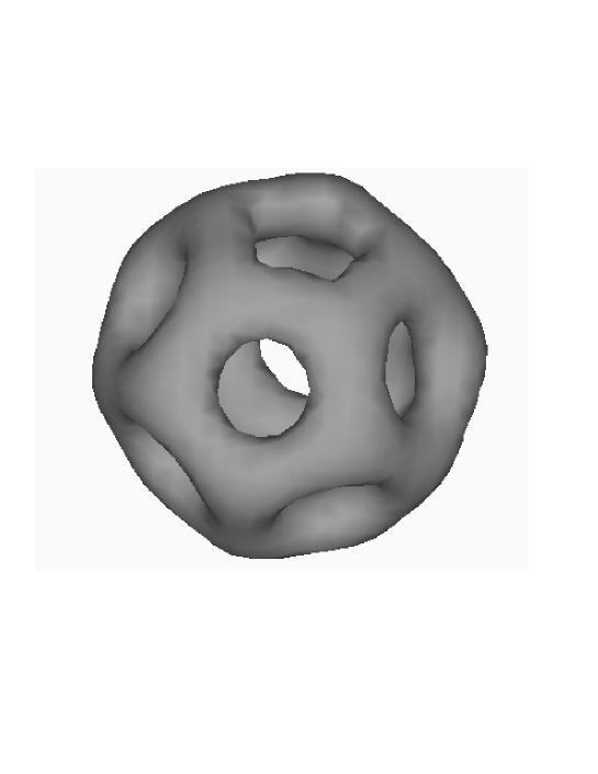
Figure 1: Dodecahedral 7-monopole; surface of constant energy density ${\cal E}=0.05$.

4 Octahedral Five Monopole

The lowest degree octahedrally invariant homogeneous polynomial is [12]

$$\zeta_{1}^{8}+14\zeta_{1}^{4}\zeta_{0}^{4}+\zeta_{0}^{8}.$$ (4.1)

Polarizing this gives

$$\xi_{1}^{2}\otimes(56\zeta_{1}^{6}+168\zeta_{1}^{2}\zeta_{0}^{4})+2\xi_{1}\xi_{0}\otimes(224\zeta_{1}^{3}\zeta_{0}^{3})+\xi_{0}^{2}\otimes(56\zeta_{0}^{6}+168\zeta_{1}^{4}\zeta_{0}^{2})$$ (4.2)

which we write in the form

$$\xi_{1}^{2}\otimes(56+\frac{7}{15}(\zeta_{0}\frac{\partial}{\partial\zeta_{1}})^{4})\zeta_{1}^{6}+2\xi_{1}\xi_{0}\otimes\frac{28}{15}(\zeta_{0}\frac{\partial}{\partial\zeta_{1}})^{3}\zeta_{1}^{6}+\xi_{0}^{2}\otimes(\frac{7}{90}(\zeta_{0}\frac{\partial}{\partial\zeta_{1}})^{6}+\frac{28}{5}(\zeta_{0}\frac{\partial}{\partial\zeta_{1}})^{2})\zeta_{1}^{6}$$ (4.3)

giving matrices

$$X\otimes(56+\frac{7}{15}(\mbox{ad}Y)^{4})X^{3}+(\mbox{ad}Y)X\otimes\frac{28}{15}(\mbox{ad}Y)^{3}X^{3}+\frac{1}{2}(\mbox{ad}Y)^{2}X\otimes(\frac{7}{90}(\mbox{ad}Y)^{6}+\frac{28}{5}(\mbox{ad}Y)^{2})X^{3}.$$ (4.4)

If we represent the $su(2)$ basis (2.5) by

$$H=\left[{\begin{array}[]{rrrrr}-4&0&0&0&0\\ 0&-2&0&0&0\\ 0&0&0&0&0\\ 0&0&0&2&0\\ 0&0&0&0&4\end{array}}\right],X=-i\left[{\begin{array}[]{ccccr}0&0&0&0&0\\ 2&0&0&0&0\\ 0&\sqrt{6}&0&0&0\\ 0&0&\sqrt{6}&0&0\\ 0&0&0&2&0\end{array}}\right],Y=i\left[{\begin{array}[]{rcccc}0&2&0&0&0\\ 0&0&\sqrt{6}&0&0\\ 0&0&0&\sqrt{6}&0\\ 0&0&0&0&2\\ 0&0&0&0&0\end{array}}\right].$$

this gives the invariant Nahm triplet in $\underline{9}_{u}$

$$Y_{1}=i\left[{\begin{array}[]{ccccc}0&-6&0&10&0\\ -6&0&2\,\sqrt{6}&0&10\\ 0&2\sqrt{6}&0&2\sqrt{6}&0\\ 10&0&2\sqrt{6}&0&-6\\ 0&10&0&-6&0\end{array}}\right],\;\;Y_{2}=\left[{\begin{array}[]{ccccc}0&-6&0&-10&0\\ 6&0&2\sqrt{6}&0&-10\\ 0&-2\sqrt{6}&0&2\sqrt{6}&0\\ 10&0&-2\sqrt{6}&0&-6\\ 0&10&0&6&0\end{array}}\right],$$

$$Y_{3}=i\left[{\begin{array}[]{ccrcc}8&0&0&0&0\\ 0&-16&0&0&0\\ 0&0&0&0&0\\ 0&0&0&16&0\\ 0&0&0&0&-8\end{array}}\right].$$

The $\underline{9}_{u}$ invariant (4.4) is written in the form (2) as

$$\left[56+\frac{7}{15}(\mbox{ad}Y\otimes 1+1\otimes\mbox{ad}Y)^{4}+\frac{1}{720}(\mbox{ad}Y\otimes 1+1\otimes\mbox{ad}Y)^{8}\right]X\otimes X^{3}$$ (4.5)

which when mapped using the isomorphism produces the invariant Nahm triplet in $\underline{9}_{m}$

$$Z_{1}=i\left[{\begin{array}[]{ccccc}0&-1&0&-1&0\\ 1&0&\sqrt{6}&0&1\\ 0&-\sqrt{6}&0&-\sqrt{6}&0\\ 1&0&\sqrt{6}&0&1\\ 0&-1&0&-1&0\end{array}}\right],\;\;Z_{2}=\left[{\begin{array}[]{rcccr}0&-1&0&1&0\\ -1&0&\sqrt{6}&0&-1\\ 0&\sqrt{6}&0&-\sqrt{6}&0\\ 1&0&-\sqrt{6}&0&1\\ 0&-1&0&1&0\end{array}}\right],$$

$$Z_{3}=i\left[{\begin{array}[]{crrrc}0&0&0&0&4\\ 0&0&0&0&0\\ 0&0&0&0&0\\ 0&0&0&0&0\\ -4&0&0&0&0\end{array}}\right].$$

In a similar fashion to the icosahedral case, we can consistently consider Nahm data of the form $T_{i}(s)=x(s)\rho_{i}+y(s)Y_{i}$. The Nahm equations become

$$\frac{dx}{ds} = 2x^{2}-48y^{2},$$ (4.6)

$$\frac{dy}{ds} = -6xy-8y^{2}$$ (4.7)

and the spectral curve is

$$\eta^{5}+768\kappa^{4}\eta(\zeta^{8}+14\zeta^{4}+1)=0$$ (4.8)

where

$$\kappa^{4}=5y(x+3y)(x-2y)^{2}.$$ (4.9)

Equations (4.6-4.7) are identical to those for the charge four cubic monopole [6] and are solved by

$$x = \frac{2\kappa(5\wp^{2}(u)-3)}{5{{\wp^{\prime}}}(u)},$$ (4.10)

$$y = \frac{2\kappa}{5{{\wp^{\prime}}}(u)},$$ (4.11)

where $u=2\kappa s$ and $\wp$ is the Weierstrass elliptic function satisfying

$${\wp^{\prime}}^{2}=4(\wp^{3}-\wp).$$ (4.12)

As in [6], the argument of $\kappa$ is chosen to be $\pi/4$ and $u$ lies on the line from $0$ to $\omega_{2}=\omega_{1}+\omega_{3}$, where $2\omega_{1}$ is the real period of the elliptic function (4.12) and $2\omega_{3}$ is the imaginary period. By examining the eigenvalues of the residue of $iT_{3}$ we see the boundary conditions at $s=0$ and $s=2$ are satisfied provided,

$$\omega_{2}=4\kappa.$$ (4.13)

This period may be explicitly calculated, with the result that there exists an octahedral monopole with spectral curve

$$\eta^{5}+\frac{3\Gamma(\frac{1}{4})^{8}}{16\pi^{2}}(\zeta^{8}+14\zeta^{4}+1)\eta=0.$$ (4.14)

Note that the spectral curve (1.10) of the cubic 4-monopole is

$$\eta^{4}+\Xi(\zeta^{8}+14\zeta^{4}+1)\eta=0$$ (4.15)

for some constant $\Xi$ and the spectral curve (4.14) of the octahedral 5-monopole is

$$\eta\left[\eta^{4}+4\Xi(\zeta^{8}+14\zeta^{4}+1)\eta\right]=0$$ (4.16)

where $\Xi$ is the same constant. The spectral curve of the octahedral 5-monopole is therefore given by a multiplication by $\eta$ of the cubic 4-monopole spectral curve, up to the factor of $4$ in the constant. Rather remarkably, this is exactly how the spectral curve of the axisymmetric 3-monopole is obtained from that of the axisymmetric 2-monopole. The two spectral curves in this case being [7]

$$\eta^{2}+\frac{\pi^{2}}{4}\zeta^{2} = 0$$ (4.17)

$$\eta\left[\eta^{2}+\pi^{2}\zeta^{2}\right] = 0.$$ (4.18)

The energy density of the 2-monopole described by (4.17) is axially symmetric, so that a surface of constant energy density is toroidal. This is also true of the 3-monopole (4.18) and the only modification is that the torus is slightly larger in size. This suggests that the octahedral 5-monopole may resemble a cube, since the cubic 4-monopole does so, with the only modification being that the cube will be slightly larger. The fact that equations (4.6-4.7) are identical to those obtained in the cubic 4-monopole reduction of Nahm’s equations also supports this hypothesis.

Using our numerical scheme, we have calculated the energy density of the octahedral 5-monopole. Fig. 2 shows a surface of constant energy density for this monopole. It resembles an octahedron (not a cube) with the energy density taking its maximum value on the six vertices of the octahedron. We found this result quite surprising, given the comments above. However, it is good news for our conjecture of Section 1, which claimed that this monopole would look like an octahedron.

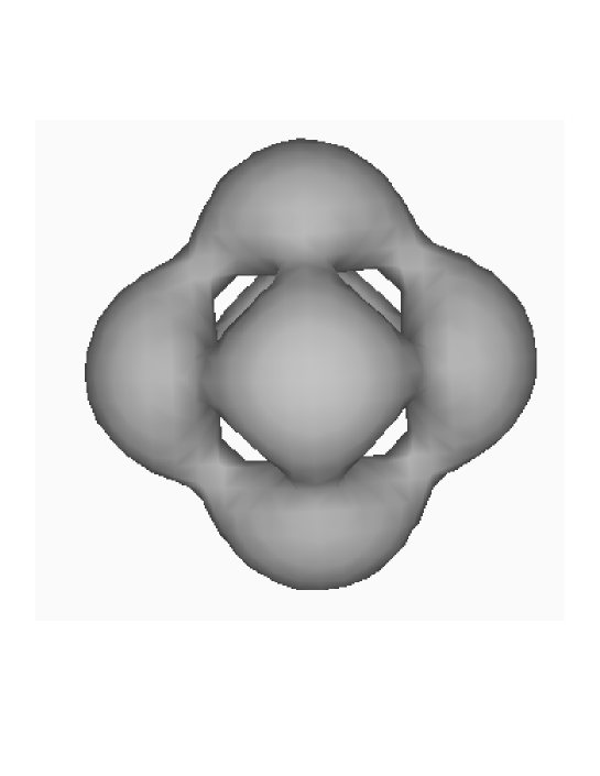
Figure 2: Octahedral 5-monopole; surface of constant energy density ${\cal E}=0.07$.

5 Rational Maps and Geodesic Scattering

The $k$-monopole moduli space ${\cal M}_{k}$ is the space of gauge inequivalent $k$-monopole solutions to the Bogomolny equation (1.1). The motion of slow moving monopoles can be approximated by geodesic motion in this moduli space [14, 18]. In this Section, we shall use rational maps to present geodesics containing the octahedral and dodecahedral monopoles.

A rational map of a $k$-monopole is a map from C     to C CIP¹ of the form

$$R(z)=\frac{p(z)}{q(z)}$$ (5.1)

where $q(z)$ is a monic polynomial of degree $k$ and $p(z)$ is a polynomial of degree less than $k$, with no factors in common with $q(z)$. Donaldson has proved [5] that every rational map arises from a unique $k$-monopole, so the space of such rational maps is diffeomorphic to ${\cal M}_{k}$.

For our purposes, the most useful way to understand the relationship between a monopole and its rational map is to follow the analysis of Hurtubise [11]. A line and an orthogonal plane in $\hbox{\upright\hbox to0.0pt{I\hss}\kern 1.7ptR}^{3}$ are chosen to give the decomposition

$$\hbox{\upright\hbox to0.0pt{I\hss}\kern 1.7ptR}^{3}\cong{\hbox to0.0pt{\hbox to0.0pt{C\hss}\kern 3.8pt\vrule height=8.0pt,width=0.4pt,depth=-0.1pt\hss}\phantom{C}}\times\hbox{\upright\hbox to0.0pt{I\hss}\kern 1.7ptR}.$$ (5.2)

For convenience, we choose the line to be the $x_{3}$-axis and denote by $z$ the complex coordinate on the $x_{1}x_{2}$-plane. Solutions to the linear differential equation (1.5)

$$(D_{A}-i\Phi)v=0$$ (5.3)

are considered along lines parallel to the $x_{3}$-axis. This equation has two independent solutions. A basis $(v_{0},v_{1})$ for the solutions can be chosen such that

$$\lim_{x_{3}\rightarrow\infty}v_{0}(x_{3})x_{3}^{\;-k/2}e^{x_{3}} = e_{0},$$ (5.4)

$$\lim_{x_{3}\rightarrow\infty}v_{1}(x_{3})x_{3}^{\;k/2}e^{-x_{3}} = e_{1}$$

where $e_{0}$, $e_{1}$ are constant in some asymptotically flat gauge. Thus $v_{0}$ is bounded and $v_{1}$ is unbounded as $x_{3}\rightarrow\infty$. Similarly, there is a basis $(v_{0}^{\prime},v_{1}^{\prime})$ such that $v_{0}^{\prime}$ is bounded and $v_{1}^{\prime}$ is unbounded as $x_{3}\rightarrow-\infty$. We consider the scattering along all lines and write

$$v_{0}^{\prime} = a(z)v_{0}+b(z)v_{1},$$ (5.5)

$$v_{0} = a^{\prime}(z)v_{0}^{\prime}+b(z)v_{1}^{\prime}.$$ (5.6)

The rational map is given by

$$R(z)=\frac{a(z)}{b(z)}.$$ (5.7)

Furthermore, since the spectral curve $P(\eta,\zeta)$ of a monopole corresponds to the bounded solutions to (1.5),

$$b(z)=P(z,0).$$ (5.8)

Finally, it can be shown, [2] pp. 127-128, that the full scattering data are given by

$$\left[\begin{array}[]{cc}a&b\\ -b^{\prime}&-a^{\prime}\end{array}\right]\left(\begin{array}[]{c}v_{0}\\ v_{1}\end{array}\right)\ =\left(\begin{array}[]{c}v_{0}^{\prime}\\ v_{1}^{\prime}\end{array}\right)$$ (5.9)

where

$$aa^{\prime}=1+b^{\prime}b.$$ (5.10)

The advantage of rational maps is that monopoles are easily described in this approach, since one simply writes down any rational map. The disadvantage is that the rational map tells us very little about the monopole. In particular, since the construction of the rational map requires the choice of a direction in $\hbox{\upright\hbox to0.0pt{I\hss}\kern 1.7ptR}^{3}$ it is not possible to study the full symmetries of a monopole from its rational map. However, the following isometries are known [6]. Let $\lambda\in U(1)$ and $\nu\in{\hbox to0.0pt{\hbox to0.0pt{C\hss}\kern 3.8pt\vrule height=8.0pt,width=0.4pt,depth=-0.1pt\hss}\phantom{C}}$ define a rotation and translation respectively in the plane C    . Let $x\in\hbox{\upright\hbox to0.0pt{I\hss}\kern 1.7ptR}$ define a translation perpendicular to the plane and let $\mu\in U(1)$ be a constant gauge transformation. Under the composition of these transformation a rational map $R(z)$ transforms as

$$R(z)\rightarrow\mu^{2}e^{2x}\lambda^{-2k}R(\lambda^{-1}(z-\nu)).$$ (5.11)

Furthermore, under space inversion, $x_{3}\rightarrow-x_{3}$, $R(z)=p(z)/q(z)$ transforms as

$$\frac{p(z)}{q(z)}\rightarrow\frac{I(p)(z)}{q(z)}$$ (5.12)

where $I(p)(z)$ is the unique polynomial of degree less than $k$ such that $(I(p)p)(z)=1$ mod $q(z)$.

We note that this implies that the rational map of a charge $L$ axisymmetric monopole lying a distance $x$ above the plane is

$$\frac{e^{2x+i\chi}}{z^{L}}$$ (5.13)

and that the full scattering data for such a monopole are

$$\left[\begin{array}[]{cc}e^{2x+i\chi}&z^{L}\\ 0&-e^{-(2x+i\chi)}\end{array}\right].$$ (5.14)

Using (5.11) and (5.12), it is easy to show that (up to a choice of orientation) the most general rational map of a strongly centred 5-monopole, which is invariant under both inversion and $C_{4}$ rotation around the $x_{3}$ axis is

$$R_{5}(z)=\frac{\frac{2}{a}z^{4}+1}{z^{5}+az}$$ (5.15)

with $a\in(0,\infty)$. It is a one parameter family of based rational maps, corresponding to geodesic scattering of 5-monopoles. Since the octahedral monopole satisfies this symmetry, it must lie on this geodesic.

Similarly, by imposing a $C_{10}$ symmetry on 7-monopoles, generated by simultaneous inversion and rotation by $\frac{\pi}{5}$, there is again a unique (up to orientation) one parameter family of maps given by

$$R_{7}(z)=\frac{az^{5}+1}{z^{7}}$$ (5.16)

with $a\in(-\infty,\infty)$. The dodecahedral monopole satisfies this symmetry and must lie somewhere on the geodesic.

We can understand these scattering processes by examining the rational maps $R_{5}(z)$ and $R_{7}(z)$ for extreme values of the parameter $a$. It is known [6, 3] that for a rational map $p(z)/q(z)$ with well separated poles $\beta_{1},\ldots,\beta_{k}$ the corresponding monopole is approximately composed of unit charge monopoles located at the points $(x_{1},x_{2},x_{3})$, where $x_{1}+ix_{2}=\beta_{i}$ and $x_{3}=\frac{1}{2}\log{|p(\beta_{i})|}$. This approximation applies only when the values of the numerator at the poles is small compared to the distance between the poles. Thus, for large values of $a$, $R_{5}(z)$ corresponds to a monopole located at the origin and a monopole a distance $\pm a$ along each of the diagonals $x_{1}=\pm x_{2}$. This interpretation breaks down for $a\sim 1$. The poles of $R_{7}(z)$ are never well separated, so there is no region in which this approximation can be applied to this rational map.

In [2] pp. 25-26 it is argued that for monopoles strung out in well separated clusters along, or nearly along, the $x_{3}$ axis the first term in a large $z$ expansion of the rational map $R(z)$ will be $e^{2x+i\chi}/z^{L}$ where $L$ is the charge of the topmost cluster and $x$ is its elevation above the plane. We would like to extend this and argue that if the next highest cluster has charge $M$ and is $y$ above the plane then the first two terms in the large $z$ expansion of the rational map will be given by

$$R(z)\sim\frac{e^{2x+i\chi}}{z^{L}}+\frac{e^{2y+i\phi}}{z^{2L+M}}+...$$ (5.17)

Assume the topmost cluster, $(A_{1},\phi_{1})$ is well separated from the other monopoles. Let $v_{0}^{\prime\prime}$ be the solution bounded at $x_{3}\rightarrow-\infty$. For $z$ large, we are considering scattering along lines well removed from the spectral lines and so in the region of $(A_{1},\phi_{1})$ the solution is dominated by the exponentially growing one and is therefore close to $v_{0}^{\prime\prime}$. Thus the dominant term in the rational map is the effect of scattering off $(A_{1},\phi_{1})$.

We now consider the second highest monopole cluster $(A_{2},\phi_{2})$. Since it is separated from the monopoles below it the incoming solution is close to $v_{0}^{\prime\prime}$. If we call the bounded solution leaving the $(A_{2},\phi_{2})$ region $v_{0}^{\prime}$ and the unbounded one $v_{1}^{\prime}$ we have from (5.14)

$$v_{0}^{\prime\prime}=e^{2y+i\phi}v_{0}^{\prime}+z^{M}v_{1}^{\prime}.$$ (5.18)

Subsequent scattering off $(A_{1},\phi_{1})$ gives

$$v_{0}^{\prime} = -e^{-2x-i\chi}v_{1}$$ (5.19)

$$v_{1}^{\prime} = e^{2x+i\chi}v_{0}+z^{L}v_{1}$$

where $v_{0}$ and $v_{1}$ are respectively the unbounded and bounded solutions as $x_{3}\rightarrow\infty$. Substituting (5.19) into (5.18) we find that

$$v_{0}^{\prime\prime}=z^{M}e^{2x+i\chi}v_{0}+(z^{M+L}-e^{-2(x-y)-i(\chi-\phi)})v_{1}$$ (5.20)

and so the rational map is dominated by

$$R(z)\sim\frac{z^{M}e^{2x+i\chi}}{z^{M+L}-e^{-2(x-y)-i(\chi-\phi)}}$$ (5.21)

and so since $x\gg y\gg 1$

$$R(z)-\frac{e^{2x+i\chi}}{z^{L}}\sim\frac{e^{2y+i\phi}}{z^{2L+M}}$$ (5.22)

as required. Obviously this type of argument could be extended to further monopoles along the line, but we do not need to do so here.

We can now see that $R_{5}(z)$ describes four monopoles approaching a monopole at the origin along the negative and positive directions of the $x_{1}$ and $x_{2}$ axis. At some point, the monopoles coalesce to form the octahedral 5-monopole. As $a\rightarrow 0$, we see from (5.17) that one monopole travels up the $x_{3}$-axis and three remain in a cluster at the origin. By inversion the fifth monopole travels down the $x_{3}$-axis. In the $a=0$ limit, there are spherical unit charge monopoles at $(0,0,\pm\infty)$ and a toroidal 3-monopole centred on the origin.

Similarly the rational map $R_{7}(z)$ corresponds to two 2-monopole clusters approaching a toroidal 3-monopole along the positive and negative $x_{3}$-axis. At some negative value of $a$, say $a=-d$, they coalesce to form a dodecahedron oriented so that two faces are parallel to the $x_{1}x_{2}$-plane. Then at $a=0$ they form a toroidal 7-monopole. At $a=d$ they form another dodecahedron, rotated $\pi/5$ relative to the previous one. Finally, for large values of $a$ the rational map corresponds to a toroidal 3-monopole at the origin and two 2-monopole clusters receding along the positive and negative $x_{3}$-axis.

Recently, we have been investigating a whole family of scattering geodesics similar to the one above. One of the interesting features of these scattering processes is the complicated motion of the zeros of the Higgs field. A detailed investigation will be presented elsewhere [10].

6 Conclusion

By explicit construction of the spectral curves, we have proved the existence of a charge seven monopole with icosahedral symmetry and a charge five monopole with octahedral symmetry. Numerical computation of the monopole energy density reveals that the former looks like a dodecahedron and the latter an octahedron. The energy density is maximal on the vertices of these two regular solids.

Using Donaldson’s rational map formulation we have presented a totally geodesic one-dimensional submanifold of the monopole moduli space which contains the dodecahedral 7-monopole and one which contains the octahedral 5-monopole. In the moduli space approximation of soliton dynamics, these submanifolds describe a new type of novel multi-monopole scattering which requires further investigation.

Acknowledgements

Many thanks to Nigel Hitchin and Nick Manton for useful discussions. CJH thanks the EPSRC for a research studentship and the British Council for a FCO award. PMS thanks the EPSRC for a research fellowship.

References

• [1] M.F. Atiyah, private communication.
• [2] M.F. Atiyah and N.J. Hitchin, β€˜The geometry and dynamics of magnetic monopoles’, Princeton University Press, 1988.
• [3] R. Bielawski, β€˜Monopoles, particles and rational functions’, McMaster preprint, 1994.
• [4] E. Braaten, S. Townsend and L. Carson, β€˜Novel structure of static multisoliton solutions in the Skyrme model’, Phys. Lett. 235B, 147 (1990).
• [5] S.K. Donaldson, β€˜Nahm’s equations and the classification of monopoles’, Commun. Math. Phys. 96, 387 (1984).
• [6] N.J. Hitchin, N.S. Manton and M.K. Murray, β€˜Symmetric monopoles’, Nonlinearity, 8, 661 (1995).
• [7] N.J. Hitchin, β€˜Monopoles and geodesics’, Commun. Math. Phys. 83, 579 (1982).
• [8] N.J. Hitchin, β€˜On the construction of monopoles’, Commun. Math. Phys. 89, 145 (1983).
• [9] C.J. Houghton and P.M. Sutcliffe, β€˜Tetrahedral and cubic monopoles’, Cambridge preprint DAMTP 95-13.
• [10] C.J. Houghton and P.M. Sutcliffe, β€˜Monopole scattering with a twist’, Cambridge preprint DAMTP 95-28.
• [11] J. Hurtubise, β€˜Monopoles and rational maps: a note on a theorem of Donaldson’, Commun. Math. Phys. 100, 463 (1985).
• [12] F. Klein, β€˜Lectures on the icosahedron’, London, Kegan Paul, 1913.
• [13] R.A. Leese and N.S. Manton, β€˜Stable instanton-generated Skrme fields with baryon numbers three and four’, Nucl. Phys. 572A, 675 (1994).
• [14] N.S. Manton, β€˜A remark on the scattering of BPS monopoles’, Phys. Lett. 110B, 54 (1982).
• [15] W. Nahm, β€˜The construction of all self-dual multimonopoles by the ADHM method’, in Monopoles in quantum field theory, eds. N.S. Craigie, P. Goddard and W. Nahm, World Scientific, 1982.
• [16] M.K. Prasad, β€˜Yang-Mills-Higgs monopole solutions of arbitrary topological charge’, Commun. Math. Phys. 80, 137 (1981).
• [17] M.K. Prasad and C.M. Sommerfield, β€˜Exact classical solution for the ’t Hooft monopole and the Julia-Zee dyon’, Phys. Rev. Lett. 35, 760 (1975).
• [18] D. Stuart, β€˜The geodesic approximation for the Yang-Mills-Higgs equation’, Commun. Math. Phys. 166, 149 (1994).
• [19] R.S. Ward, β€˜A Yang-Mills-Higgs monopole of charge two’, Commun. Math. Phys. 79, 317 (1981);Β
• [20] R.S. Ward, β€˜Two Yang-Mills-Higgs monopoles close together’, Phys. Lett. B102, 136 (1981).