DAMTP 95-13 To appear in Communications in Mathematical Physics
Tetrahedral and Cubic Monopoles

Abstract

Using a numerical implementation of the ADHMN construction, we compute the fields and energy densities of a charge three monopole with tetrahedral symmetry and a charge four monopole with octahedral symmetry. We then construct a one parameter family of spectral curves and Nahm data which represent charge four monopoles with tetrahedral symmetry, which includes the monopole with octahedral symmetry as a special case. In the moduli space approximation, this family describes a novel kind of four monopole scattering and we use our numerical scheme to construct the energy density at various times during the motion.

1 Introduction

BPS monopoles are topological solitons in a Yang-Mills-Higgs gauge theory in three space dimensions. The equation for static monopoles is integrable, so that a variety of techniques are available for studying monopoles and constructing solutions. Monopoles of charge one and two are well-understood, with explicit solutions known, but for higher charges the situation is not so clear. Despite the integrability of the equation, explicit solutions for charge three and above are known only in the axisymmetric case, which corresponds to coincident monopoles. Very recently, some progress has been made in this area [1] with existence proofs for a charge three monopole with tetrahedral symmetry and a charge four monopole with octahedral symmetry. In this paper, we compute these monopoles using a numerical implementation of the Atiyah-Drinfeld-Hitchin-Manin-Nahm (ADHMN) construction and display their energy densities.

When time dependence is introduced, the monopole equation of motion is not integrable. However, analytical progress can still be made, via the moduli space approximation [2], from knowledge of the static monopoles. This has been extensively studied for the case of charge two monopole scattering [3], but the extension to higher charges has proved a less tractable problem. We have made some progress in this area and present our results on a particularly symmetric example of charge four monopole scattering. The charge four monopole has tetrahedral symmetry throughout the motion, which is the key to our construction of the relevant spectral curves and Nahm data. We use our numerical scheme to display the energy density at various times.

2 Monopoles, spectral curves and Nahm data

In this paper, we study solutions of the Bogomolny equation

$$D_{i}\Phi=-\frac{1}{2}\epsilon_{ijk}F_{jk}$$ (2.1)

for SU(2) BPS monopoles in IR³. Here $D_{i}=\frac{\partial}{\partial x_{i}}+[A_{i},$  is the covariant derivative with $A_{i}$ the su(2)-valued gauge potential and $F_{jk}$ the gauge field. $\Phi$ is the Higgs field, which is an su(2)-valued scalar field satisfying the boundary condition

$$\|\Phi\|=1-\frac{k}{r}+O(\frac{1}{r^{2}})\hskip 10.0pt\mbox{as}\hskip 10.0ptr\rightarrow\infty$$ (2.2)

where $r=|\mbox{\boldmath$x$}|$, $\|\Phi\|^{2}=-\frac{1}{2}\mbox{tr}\Phi^{2}$ and $k$ is a positive integer, known as the magnetic charge. We shall refer to a monopole with magnetic charge $k$ as a $k$-monopole. The energy density, ${\cal E}$, of a monopole is given by

$${\cal E}=-\frac{1}{2}\mbox{tr}(D_{i}\Phi)(D_{i}\Phi)-\frac{1}{4}\mbox{tr}(F_{ij}F_{ij}).$$ (2.3)

The energy is the integral of ${\cal E}$ over all space and is equal to $8\pi k$.

Equation (2.1) may be obtained by dimensional reduction of the self-dual Yang-Mills equation in IR⁴, for which there is a well-known twistor correspondence; namely that solutions of the self-duality equations correspond to certain holomorphic vector bundles over the standard complex 3-dimensional twistor space. This correspondence may be reduced [4, 5, 6] to give that monopoles correspond to particular holomorphic vector bundles over a mini-twistor space TT, which is a 2-dimensional complex manifold isomorphic to the holomorphic tangent bundle to the Riemann sphere ie TT$\cong$TC CIP¹. Moreover, the bundle (and hence the monopole) is determined by an algebraic curve in TT, called the spectral curve, which must satisfy certain reality and non-singularity conditions.

The space TT is a fibre bundle over C CIP¹ with each fibre being a copy of C C. Let $\zeta$ be the standard coordinate on the base space and $\eta$ the fibre coordinate, then the three spectral curves of interest in this paper are

$$\eta^{3} +i\frac{\Gamma(1/6)^{3}\Gamma(1/3)^{3}}{48\sqrt{3}\pi^{3/2}}\zeta(\zeta^{4}-1)=0$$ (2.4)

$$\eta^{4} +\frac{3\Gamma(1/4)^{8}}{64\pi^{2}}(\zeta^{8}+14\zeta^{4}+1)=0$$ (2.5)

$$\eta^{4} +i36a\kappa^{3}\eta\zeta(\zeta^{4}-1)+3\kappa^{4}(\zeta^{8}+14\zeta^{4}+1)=0.$$ (2.6)

In [1] it is proved that (2.4) is the spectral curve of a 3-monopole with tetrahedral symmetry and that (2.5) is the spectral curve of a 4-monopole with octahedral symmetry. It is the monopole fields and energy densities which correspond to these two spectral curves that we shall compute numerically in Section 3. In Section 4 we shall prove that (2.6) is the spectral curve of a 4-monopole with tetrahedral symmetry for all $a\in(-3^{-5/4}\sqrt{2},3^{-5/4}\sqrt{2})$ where $2\kappa$ is the real period of the elliptic curve

$$y^{2}=4(x^{3}-x+3a^{2}).$$ (2.7)

If $a=0$ then (2.6) becomes (2.5), so that at this point the 4-monopole has octahedral symmetry.

Although the spectral curve approach to monopoles is a very useful and powerful technique, its main drawback is that the non-singularity constraint, which an algebraic curve must satisfy to be the spectral curve of a monopole, is rather formidable to check. However, there is an alternative approach to the construction of monopoles which nicely complements the spectral curve formulation, in the sense that the non-singularity of the monopole is automatic. The ADHMN construction [7, 6] is an equivalence between $k$-monopoles and Nahm data $(T_{1},T_{2},T_{3})$, which are three $k\times k$ matrices which depend on a real parameter $s\in[0,2]$ and satisfy the following;

(i) Nahm’s equation

$$\frac{dT_{i}}{ds}=\frac{1}{2}\epsilon_{ijk}[T_{j},T_{k}]$$

(ii) $T_{i}(s)$ is regular for $s\in(0,2)$ and has simple poles at $s=0$ and $s=2$,

(iii) the matrix residues of $(T_{1},T_{2},T_{3})$ at each pole form the irreducible $k$-dimensional representation of SU(2),

(iv) $T_{i}(s)=-T_{i}^{\dagger}(s)$,

(v) $T_{i}(s)=T_{i}^{t}(2-s)$.

Equation (i) is equivalent to a Lax pair and hence there is an associated algebraic curve, which is in fact the spectral curve. Explicitly, the spectral curve may be read off from the Nahm data as the equation

$$\mbox{det}(\eta+(T_{1}+iT_{2})-2iT_{3}\zeta+(T_{1}-iT_{2})\zeta^{2})=0.$$ (2.8)

In Section 3, we review how to obtain the monopole fields from the Nahm data and explain our numerical implementation of this procedure.

3 Numerical ADHMN construction

Finding the Nahm data effectively solves the nonlinear part of the monopole construction but in order to calculate the fields themselves the linear part of the ADHMN construction must also be implemented [7, 6]. Given Nahm data $(T_{1},T_{2},T_{3})$ for a $k$-monopole we must solve the ordinary differential equation (ODE)

$$({{\upright\hbox to0.0pt{1\hss}\kern 2.0pt1}}_{2k}\frac{d}{ds}+{{\upright\hbox to0.0pt{1\hss}\kern 2.0pt1}}_{k}\otimes x_{j}\sigma_{j}+iT_{j}\otimes\sigma_{j}){\bf v}=0$$ (3.1)

for the complex $2k$-vector ${\bf v}(s)$, where ${\upright\hbox to0.0pt{1\hss}\kern 2.0pt1}_{k}$ denotes the $k\times k$ identity matrix, $\sigma_{j}$ are the Pauli matrices and ${\bf x}=(x_{1},x_{2},x_{3})$ is the point in space at which the monopole fields are to be calculated. Introducing the inner product

$$\langle{\bf v}_{1},{\bf v}_{2}\rangle=\int_{0}^{2}{\bf v}_{1}^{\dagger}{\bf v}_{2}\ ds$$ (3.2)

then the solutions of (3.1) which we require are those which are normalizable with respect to (3.2). It can be shown that the space of normalizable solutions to (3.1) has (complex) dimension 2. If $\widehat{\bf v}_{1},\widehat{\bf v}_{2}$ is an orthonormal basis for this space then the Higgs field $\Phi$ is given by

$$\Phi=i\left[\begin{array}[]{cc}\langle(s-1)\widehat{\bf v}_{1},\widehat{\bf v}_{1}\rangle&\langle(s-1)\widehat{\bf v}_{1},\widehat{\bf v}_{2}\rangle\\ \langle(s-1)\widehat{\bf v}_{2},\widehat{\bf v}_{1}\rangle&\langle(s-1)\widehat{\bf v}_{2},\widehat{\bf v}_{2}\rangle\end{array}\right].$$ (3.3)

There is a similar expression for the gauge potential but we shall not need this here. In some cases this procedure, which goes from Nahm data to the Higgs field, may be completed analytically to give an explicit closed form for $\Phi$. However, the Nahm data which we consider in this paper is sufficiently complicated that to calculate a closed form expression for $\Phi$ appears not to be a tractable problem. We therefore turn to a numerical implementation of the above procedure, which we now describe.

The first issue we confront in a numerical approach is to calculate numerical values for the Nahm data on the interval $s\in[0,2]$. Although we shall have explicit expressions for the Nahm data this is still not quite a trivial issue, since the expressions involve the Weierstrass elliptic function $\wp$ and its derivative. However, we can keep the number of calculations of $T_{i}(s)$ to a minimum by noting that if a fixed step ODE solver is used to integrate (3.1) then the Nahm data is required at the same $s$ values for every integration of (3.1) for all initial conditions and ${\bf x}$ positions. Therefore we compute, once and for all, $T_{i}(s)$ at $2P$ equidistant points for $s\in[0,2]$ and store these values, which are then used as a look-up table when integrating (3.1) by a fourth order Runge-Kutta method with fixed steplength $ds=2P^{-1}$. The values in the look-up table are computed from the closed form expressions using MATHEMATICA.

Let $\Omega(I)$ denote the space of solutions to (3.1) which are normalizable for $s$ in the interval $I$. Then we require a basis for the 2-dimensional space $\Omega([0,2])$. The question we now address is how to obtain this basis from solutions of the initial value problem (IVP) associated with the ODE (3.1). Consider the IVP of (3.1) at the pole $s=0$, which has the form

$$s\frac{d{\bf v}}{ds}=B_{s}{\bf v}$$ (3.4)

where $B_{s}$ is a regular $2k\times 2k$ matrix function of $s\in[0,2)$. This is a regular-singular problem so that $\Omega([0,2))$ has dimension $N$, where $N$ is the number of positive eigenvalues (counted with multiplicity) of $B_{0}$. If $N$ was equal to 2 then we could easily compute a basis for $\Omega([0,2])$ since it would (almost) be given by a basis for $\Omega([0,2))$, which can be found by integrating (3.1), as described above, with two different initial conditions. However, for all the cases considered in this paper we find $N>2$, so that the problem requires a little more work. By symmetry of the Nahm data, if we consider the IVP of (3.1) at the pole $s=2$ (with $ds<0$) then we have a similar regular-singular problem involving a matrix which again has $N$ positive eigenvalues. By integrating this IVP we can compute a basis for the $N$-dimensional space $\Omega((0,2])$. The 2-dimensional space we require is the intersection of the above two $N$-dimensional spaces ie

$$\Omega([0,2])=\Omega([0,2))\cap\Omega((0,2]).$$ (3.5)

To find the intersection of these two spaces is a shooting problem but because the ODE (3.1) is linear this shooting problem can be reduced to linear algebra as follows. Let ${\bf u}_{1}(s),{\bf u}_{2}(s),..,{\bf u}_{N}(s)$ denote $N$ $2k$-vectors which form a basis for $\Omega([0,2))$ and

${\bf u}_{N+1}(s),{\bf u}_{N+2}(s),..,{\bf u}_{2N}(s)$ a basis for $\Omega((0,2])$. Explicitly these vectors are computed by solving the IVP at $s=0$ and $s=2$ with $N$ different initial conditions each. Define the $2k\times 2N$ matrix

$$U=\left[\begin{array}[]{cccc}|&|&&|\\ |&|&&|\\ {\bf u}_{1}(1)&{\bf u}_{2}(1)&...&{\bf u}_{2N}(1)\\ |&|&&|\\ |&|&&|\end{array}\right]$$ (3.6)

then we need to find a basis for the 2-dimensional kernel of $U$ ie to solve the matrix equation

$$U{\bf w}={\bf 0}$$ (3.7)

for ${\bf w}=(w_{1},...,w_{2N})\neq{\bf 0}$. Numerically this is performed by row reduction of the matrix $U$ followed by back substitution. Let ${\bf w}^{(1)}$ and ${\bf w}^{(2)}$ denote two independent solutions to (3.7), then a basis for $\Omega([0,2])$ is given by

$${\bf v}_{l}(s)=\left\{\begin{array}[]{ll}\ \sum_{j=1}^{N}{\bf w}_{j}^{(l)}{\bf u}_{j}(s)&\mbox{if $0\leq s\leq 1$}\\ &\\ -\sum_{j=N+1}^{2N}{\bf w}_{j}^{(l)}{\bf u}_{j}(s)&\mbox{if $1<s\leq 2$}\end{array}\right.$$ (3.8)

for $l=1,2$. To summarize, the above procedure consists in integrating (3.1) $N$ times from each end of the interval $[0,2]$ to the centre and then finding linear combinations of these solutions such that these combinations, which start at each end of the interval, match at the centre.

Given ${\bf v}_{1}$ and ${\bf v}_{2}$ we use the Gram-Schmidt orthonormalization algorithm, with inner product (3.2) (and the integral calculated from the $P$ data values via a simple Simpsons rule), to obtain two orthonormal vectors $\widehat{\bf v}_{1},\widehat{\bf v}_{2}$. The Higgs field $\Phi$ is then computed according to (3.3) and to calculate the energy density we make use of the formula

$${\cal E}=\bigtriangleup\|\Phi\|^{2}$$ (3.9)

where $\bigtriangleup$ denotes the laplacian on IR³. Numerically we use the above scheme to calculate $\|\Phi\|^{2}$ on a spatial lattice of $M\times M\times M$ points and approximate the laplacian in (3.9) using a finite difference method with a 7-point stencil. This completes our numerical ADHMN algorithm.

Although every stage of our algorithm is a relatively inexpensive computing task each must be executed many times to build up a detailed picture of the energy density. To produce each of the energy density plots appearing later in the paper we used the values $P=50$ and $M=31$, with $(x_{1},x_{2},x_{3})\in[-5,5]\times[-5,5]\times[-5,5]$. This means that the ODE (3.1) must be solved to the order of $10^{5}$ times to produce one energy density plot. Implementing our scheme on a workstation gave a run time of approximately 30 minutes to produce the data for each plot.

The Nahm data which correspond to the spectral curves (2.4) and (2.5), of a 3-monopole with tetrahedral symmetry and a 4-monopole with octahedral symmetry respectively, is given in [1] and we shall make use of it now. The method used to obtain these data is reviewed in Section 4 when we shall use it to calculate the Nahm data for the spectral curve (2.6). Not all the Nahm data given in [1] explicitly satisfies conditions (iv) and (v) given earlier. However the properties of the associated spectral curves implies that there exists a constant $k\times k$ matrix in each case such that conjugation of the Nahm data by this matrix produces equivalent Nahm data which does satisfy the conditions, and this is enough. Conjugation by a matrix is equivalent to a change of basis for the $k$-dimensional representation of SU(2) formed by the matrix residues of $(T_{1},T_{2},T_{3})$ at the $s=0$ pole. For our purposes it is convenient if this is a real representation and so (if necessary) we make a transformation to achieve this. In the case $k=3$ the Nahm data from [1] is equivalent to

$$T_{1}=\left[\begin{array}[]{ccc}0&0&0\\ 0&0&-z\\ 0&\bar{z}&0\end{array}\right]\;\;T_{2}=\left[\begin{array}[]{ccc}0&0&-\bar{z}\\ 0&0&0\\ z&0&0\end{array}\right]\;\;T_{3}=\left[\begin{array}[]{ccc}0&z&0\\ -\bar{z}&0&0\\ 0&0&0\end{array}\right]$$ (3.10)

where

$$z=\frac{\omega\wp^{\prime}(\omega s)}{2\wp(\omega s)}+\frac{\sqrt{3}\omega}{\wp(\omega s)}\mbox{ , }\;\;\omega=e^{i\pi/6}\frac{\Gamma(1/6)\Gamma(1/3)}{12\sqrt{\pi}}$$ (3.11)

and $\wp$ is the Weierstrass function satisfying

$$\wp^{\prime 2}=4\wp^{3}-4$$ (3.12)

where ^′ denotes differentiation with respect to the argument.

With this Nahm data equation (3.1) is equivalent to the set of coupled ODE’s

$$\dot{v}_{1}+x_{3}v_{1}+(x_{1}+ix_{2})v_{2}+izv_{3}-\bar{z}v_{6}=0$$

$$\dot{v}_{2}-x_{3}v_{2}+(x_{1}-ix_{2})v_{1}-izv_{4}+\bar{z}v_{5}=0$$

$$\dot{v}_{3}+x_{3}v_{3}+(x_{1}+ix_{2})v_{4}-i\bar{z}v_{1}-izv_{6}=0$$ (3.13)

$$\dot{v}_{4}-x_{3}v_{4}+(x_{1}-ix_{2})v_{3}+i\bar{z}v_{2}-izv_{5}=0$$

$$\dot{v}_{5}+x_{3}v_{5}+(x_{1}+ix_{2})v_{6}+zv_{2}+i\bar{z}v_{4}=0$$

$$\dot{v}_{6}-x_{3}v_{6}+(x_{1}-ix_{2})v_{5}-zv_{1}+i\bar{z}v_{3}=0$$

where $\dot{v}_{1}=\frac{dv_{1}}{ds}$ etc. In terms of the notation introduced earlier we find that the matrix $B_{0}$ has eigenvalues $\{1,1,1,1,-2,-2\}$ so that $N=4$.

Figure 1. displays the output of our algorithm for this case. The plot shows a surface of constant energy density ${\cal E}=0.20$. The tetrahedral symmetry of this surface is clearly evident and plots for other values of ${\cal E}$ close to this one are qualitatively similar. For large values of ${\cal E}$ the surface breaks up into four disconnected pieces centered on the vertices of a regular tetrahedron.

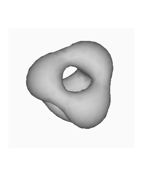
Figure 1: Tetrahedral 3-monopole; surface of constant energy density ${\cal E}=0.20$.

We now turn to the 4-monopole with octahedral symmetry. The Nahm data from [1] (after a change of basis) is

$$T_{1}=i\left[\begin{array}[]{cccc}0&\sqrt{3}(2y-x)&0&-10y\\ \sqrt{3}(2y-x)&0&-6y-2x&0\\ 0&-6y-2x&0&\sqrt{3}(2y-x)\\ -10y&0&\sqrt{3}(2y-x)&0\end{array}\right]$$

$$T_{2}=\left[\begin{array}[]{cccc}0&\sqrt{3}(2y-x)&0&10y\\ -\sqrt{3}(2y-x)&0&-6y-2x&0\\ 0&6y+2x&0&\sqrt{3}(2y-x)\\ -10y&0&-\sqrt{3}(2y-x)&0\end{array}\right]$$

$$T_{3}=i\left[\begin{array}[]{cccc}-4y-3x&0&0&0\\ 0&12y-x&0&0\\ 0&0&-12y+x&0\\ 0&0&0&4y+3x\end{array}\right]$$ (3.14)

where

$$x=\omega e^{i\pi/4}\frac{(5\wp^{2}(s\omega e^{i\pi/4}/2)-3)}{10\wp^{\prime}(s\omega e^{i\pi/4}/2)},\ y=\omega e^{i\pi/4}\frac{1}{10\wp^{\prime}(s\omega e^{i\pi/4}/2)},\ \omega=\frac{\Gamma(1/4)^{2}}{\sqrt{8\pi}}$$ (3.15)

and $\wp$ is the Weierstrass function satisfying

$$\wp^{\prime 2}=4\wp^{3}-4\wp.$$ (3.16)

Then equation (3.1) is equivalent to

$$\dot{v}_{1}+x_{3}v_{1}+(x_{1}+ix_{2})v_{2}+(4y+3x)v_{1}+20yv_{8}=0$$

$$\dot{v}_{2}-x_{3}v_{2}+(x_{1}-ix_{2})v_{1}-(4y+3x)v_{2}+2\sqrt{3}(-2y+x)v_{3}=0$$

$$\dot{v}_{3}+x_{3}v_{3}+(x_{1}+ix_{2})v_{4}+2\sqrt{3}(-2y+x)v_{2}+(-12y+x)v_{3}=0$$

$$\dot{v}_{4}-x_{3}v_{4}+(x_{1}-ix_{2})v_{3}+(12y-x)v_{4}+4(3y+x)v_{5}=0$$

$$\dot{v}_{5}+x_{3}v_{5}+(x_{1}+ix_{2})v_{6}+4(3y+x)v_{4}+(12y-x)v_{5}=0$$

$$\dot{v}_{6}-x_{3}v_{6}+(x_{1}-ix_{2})v_{5}+(-12y+x)v_{6}+2\sqrt{3}(-2y+x)v_{7}=0$$

$$\dot{v}_{7}+x_{3}v_{7}+(x_{1}+ix_{2})v_{8}+2\sqrt{3}(-2y+x)v_{6}-(4y+3x)v_{7}=0$$

$$\dot{v}_{8}-x_{3}v_{8}+(x_{1}-ix_{2})v_{7}+20yv_{1}+(4y+3x)v_{8}=0.$$

We find that the matrix $B_{0}$ has eigenvalues $\{\frac{3}{2},\frac{3}{2},\frac{3}{2},\frac{3}{2},\frac{3}{2},-\frac{5}{2},-\frac{5}{2},-\frac{5}{2}\}$, so that $N=5$.

Figure 2. displays the output of our algorithm in this case. The plot shows a surface of constant energy density ${\cal E}=0.14$. Note that for the monopole with octahedral symmetry a constant energy density surface could have resembled an octahedron or a cube; clearly it is the latter. It is therefore more natural to refer to this monopole not as an octahedral monopole but as a cubic monopole. For large values of ${\cal E}$ the surface breaks up into eight disconnected pieces on the vertices of a cube.

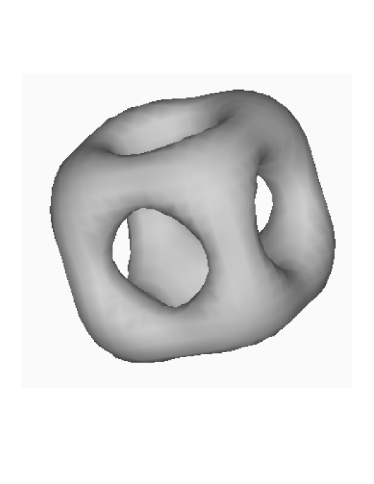
Figure 2: Cubic 4-monopole; surface of constant energy density ${\cal E}=0.14$.

4 Four Monopole Scattering

In this Section we shall use the method of [1] to construct a one parameter family of Nahm data, which represent four monopoles with tetrahedral symmetry. The imposition of tetrahedral symmetry facilitates the solving of Nahm’s equations, since we will only have to consider Nahm data which are invariant under the action of the tetrahedral group $T\subset SO(3)$.

The Nahm data are an IR${}^{3}\otimes sl(k,{\hbox to0.0pt{\hbox to0.0pt{C\hss}\kern 3.8pt\vrule height=8.0pt,width=0.4pt,depth=-0.1pt\hss}\phantom{C}})$ valued function of $s$, which transform under the rotation group $SO(3)$ as

$$\underline{3}\otimes sl(\underline{k})$$ (4.1)

where $\underline{r}$ denotes the unique irreducible r dimensional representation of $su(2)$. Since $gl(\underline{k})\cong\underline{k}\otimes\underline{k}$ Clebsh-Gordon decomposition gives

$$gl(\underline{k})\cong\underline{2k-1}\oplus\underline{2k-3}\oplus\ldots\oplus\underline{3}\oplus\underline{1}$$

and so

$$sl(\underline{k})\cong\underline{2k-1}\oplus\underline{2k-3}\oplus\ldots\oplus\underline{3}$$ (4.2)

Substituting into (4.1)

$$\underline{3}\otimes sl(\underline{k}) \cong \underline{3}\otimes(\underline{2k-1}\oplus\underline{2k-3}\oplus\ldots\oplus\underline{3})$$ (4.3)

$$\cong (\underline{2k+1}\oplus\underline{2k-1}\oplus\underline{2k-3})\oplus\ldots\oplus(\underline{5}\oplus\underline{3}\oplus\underline{1}).$$

Thus the Nahm data corresponding to four monopoles are in the carrier space $(\underline{9}\oplus\underline{7}\oplus\underline{5})\oplus(\underline{7}\oplus\underline{5}\oplus\underline{3})\oplus(\underline{5}\oplus\underline{3}\oplus\underline{1})$. The $\underline{1}$ representation is, of course, invariant under all of $SO(3)$. We will calculate this and the other tetrahedral invariants.

Write $X,Y$ and $H$ for the basis of $su(2)$ satisfying the commutation relations

$$[X,Y]=H;\qquad[H,X]=2X;\qquad[H,Y]=-2Y.$$ (4.4)

These may be represented by the principal $su(2)$ subalgebra of $sl(\underline{k})$ which in turn acts on the algebra by the adjoint action. In this representation $X$ is a rank $k-1$ nilpotent element and a basis of $sl(\underline{k})$ can be generated by acting with $Y$ on $X^{r}$, for $r=1,2,..,k-1$. Thus

$X^{k-1}$	$(adY)X^{k-1}$	$(adY)^{2}X^{k-1}$	…	…	$(adY)^{2k-2}X^{k-1}$
⋮	…
$X^{r}$	$(adY)X^{r}$	$(adY)^{2}X^{r}$	…	$(adY)^{2r}X^{r}$
⋮	…
$X$	$(adY)X$	$(adY)^{2}X$

is a basis of $sl(\underline{k})$. The element $X^{r}$ of the abelian nilpotent subalgebra $\langle X,X^{2},\ldots\,X^{k-1}\rangle$ is the highest weight vector for the $su(2)$ representation $\underline{2r+1}$ lying in the decomposition (4.2) of $sl(\underline{k})$.

It is convenient to exploit the representations of $su(2)$ on homogeneous polynomials over C CIP¹ since the invariant homogeneous polynomials are known [8], and also it connects with the spectral curve approach. The $r+1$ dimensional $su(2)$ representation $\underline{r+1}$ is defined on degree $r$ homogeneous polynomials by the identification

$$X=\zeta_{1}\frac{\partial}{\partial\zeta_{0}};\qquad Y=\zeta_{0}\frac{\partial}{\partial\zeta_{1}};\qquad H=-\zeta_{0}\frac{\partial}{\partial\zeta_{0}}+\zeta_{1}\frac{\partial}{\partial\zeta_{1}}.$$ (4.5)

In the case of degree $r$ homogeneous polynomials we can identify highest weight vector $\zeta_{1}^{r}$ and basis $\{\zeta_{1}^{r},(\zeta_{0}\frac{\partial}{\partial\zeta_{1}})\zeta_{1}^{r},\/\ldots\/,(\zeta_{0}\frac{\partial}{\partial\zeta_{1}})^{r}\zeta_{1}^{r})\}$. Thus we can relate a degree $2r$ homogeneous polynomial $q_{2r}(\zeta_{0},\zeta_{1})$ and a matrix $S$ in the $\underline{2r+1}$ representation of the decomposition of $sl(\underline{k})$ by rewriting $q_{2r}(\zeta_{0},\zeta_{1})$ as $q_{2r}(\zeta_{0}\frac{\partial}{\partial\zeta_{1}})\zeta_{1}^{2r}$ and then letting

$$S=q_{2r}(adY)X^{r}.$$ (4.6)

The lowest degree $T$-invariant polynomial is of degree $6$. It is

$$\zeta_{1}^{5}\zeta_{0}-\zeta_{1}\zeta_{0}^{5}.$$ (4.7)

There is a degree $8$ $T$-invariant polynomial

$$\zeta_{1}^{8}+14\zeta_{1}^{4}\zeta_{0}^{4}+\zeta_{0}^{8}$$ (4.8)

which is also invariant under the octahedral group. Thus, in addition to the $SO(3)$ invariant there are $T$-invariant Nahm triplets lying in the $\underline{9}$ representation and in both the $\underline{7}$ representations. It is convenient to write $(\underline{9}_{u}\oplus\underline{7}_{m}\oplus\underline{5}_{l})\oplus(\underline{7}_{u}\oplus\underline{5}_{m}\oplus\underline{3}_{l})\oplus(\underline{5}_{u}\oplus\underline{3}_{m}\oplus\underline{1}_{l})$ so that we may distinguish $\underline{7}_{m}$ and $\underline{7}_{u}$.

We can now construct the $T$-invariant Nahm triplets in $\underline{9}_{u}$ and $\underline{7}_{u}$ by (4.6) and the inclusion

$$\underline{2r+1} \hookrightarrow \underline{3}\otimes\underline{2r-1}\cong\underline{2r+1}\oplus\underline{2r-1}\oplus\underline{2r-3}$$

$$p_{2r}(\zeta_{0},\zeta_{1}) \mapsto \xi_{1}^{2}\otimes\frac{\partial^{2}p_{2r}}{\partial\zeta_{1}^{2}}+2\xi_{0}\xi_{1}\otimes\frac{\partial^{2}p_{2r}}{\partial\zeta_{0}\partial\zeta_{1}}+\xi_{0}^{2}\otimes\frac{\partial^{2}p_{2r}}{\partial\zeta_{0}^{2}}.$$ (4.9)

We choose matrices

$$X=\left[\begin{array}[]{rcrc}0&\sqrt{3}&0&0\\ 0&0&2&0\\ 0&0&0&\sqrt{3}\\ 0&0&0&0\end{array}\right]\;Y=\left[\begin{array}[]{crcr}0&0&0&0\\ \sqrt{3}&0&0&0\\ 0&2&0&0\\ 0&0&\sqrt{3}&0\end{array}\right]\;\\ H=\left[\begin{array}[]{rrrr}3&0&0&0\\ 0&1&0&0\\ 0&0&-1&0\\ 0&0&0&-3\end{array}\right].$$ (4.10)

Polarizing (4.7) yields

$$\xi_{1}^{2}\otimes(20\zeta_{1}^{3}\zeta_{0})+2\xi_{1}\xi_{0}\otimes(5\zeta_{1}^{4}-5\zeta_{0}^{4})-\xi_{0}^{2}\otimes(20\zeta_{1}\zeta_{0}^{3})$$ (4.11)

which we put into the form

$$\xi_{1}^{2} \otimes 5(\zeta_{0}\frac{\partial}{\partial\zeta_{1}})\zeta_{1}^{4}+(\xi_{0}\frac{\partial}{\partial\xi_{1}})\xi_{1}^{2}\otimes[5-\frac{5}{24}(\zeta_{0}\frac{\partial}{\partial\zeta_{1}})^{4}]\zeta_{1}^{4}$$ (4.12)

$$+ \frac{1}{2}(\xi_{0}\frac{\partial}{\partial\xi_{1}})^{2}\xi_{1}^{2}\otimes[-\frac{5}{6}(\zeta_{0}\frac{\partial}{\partial\zeta_{1}})^{3}\zeta_{1}^{4}]$$

and convert to $k\times k$ matrices

$$X\otimes 5adYX^{2}+adYX\otimes[5-\frac{5}{24}(adY)^{4}]X^{2}+\frac{1}{2}(adY)^{2}X\otimes[-\frac{5}{6}(adY)^{3}]X^{2}.$$ (4.13)

These matrices were calculated explicitly using MAPLE and are proportional to

$$Z_{1}=\left[{\begin{array}[]{rcrc}0&2\sqrt{3}&0&0\\ 0&0&0&0\\ 0&0&0&-2\sqrt{3}\\ 0&0&0&0\end{array}}\right]\;Z_{2}=\left[{\begin{array}[]{cccc}0&0&\sqrt{3}&0\\ 0&0&0&\sqrt{3}\\ -\sqrt{3}&0&0&0\\ 0&-\sqrt{3}&0&0\end{array}}\right]\;Z_{3}=\left[{\begin{array}[]{crcr}0&0&0&0\\ \sqrt{3}&0&0&0\\ 0&0&0&0\\ 0&0&-\sqrt{3}&0\end{array}}\right]\\$$ (4.14)

Similarly polarizing (4.8) yields

$$\xi_{1}^{2}\otimes(56\zeta_{1}^{6}+168\zeta_{1}^{2}\zeta_{0}^{4})+2\xi_{1}\xi_{0}\otimes(224\zeta_{1}^{3}\zeta_{0}^{3})+\xi_{0}^{2}\otimes(168\zeta_{1}^{4}\zeta_{0}^{2}+56\zeta_{0}^{6})$$ (4.15)

which becomes

$$\xi_{1}^{2} \otimes [56+\frac{7}{15}(\zeta_{0}\frac{\partial}{\partial\zeta_{1}})^{4}]\zeta_{1}^{6}+(\xi_{0}\frac{\partial}{\partial\xi_{1}})\xi_{1}^{2}\otimes\frac{28}{15}(\zeta_{0}\frac{\partial}{\partial\zeta_{1}})^{3}\zeta_{1}^{6}$$ (4.16)

$$+ \frac{1}{2}(\xi_{0}\frac{\partial}{\partial\xi_{1}})^{2}\xi_{1}^{2}\otimes[\frac{28}{5}(\zeta_{0}\frac{\partial}{\partial\zeta_{1}})^{2}+\frac{7}{90}(\zeta_{0}\frac{\partial}{\partial\zeta_{1}})^{6}]\zeta_{1}^{6}$$

yielding invariant Nahm triplet

$$Y_{1}=\left[{\begin{array}[]{crcr}0&0&0&-20\\ 4\,\sqrt{3}&0&0&0\\ 0&-12&0&0\\ 0&0&4\,\sqrt{3}&0\end{array}}\right]\;\;Y_{2}=\left[{\begin{array}[]{rrrr}-4&0&0&0\\ 0&12&0&0\\ 0&0&-12&0\\ 0&0&0&4\end{array}}\right]\;\;$$

$$Y_{3}=\left[{\begin{array}[]{rcrc}0&-2\,\sqrt{3}&0&0\\ 0&0&6&0\\ 0&0&0&-2\,\sqrt{3}\\ 10&0&0&0\end{array}}\right]$$ (4.17)

We calculate the $T$-invariant in $\underline{7}_{m}$ by constructing an isomorphism between it and $\underline{7}_{u}$. We observe that $X\otimes X^{r}$ is a highest weight vector of the representation $\underline{2r+3}_{u}$ and a basis can be generated by successive application of $(adY\otimes 1+1\otimes adY)$. Thus, for example, the invariant (4.13) can be written

$$[5(adY\otimes 1+1\otimes adY)-\frac{1}{24}(adY\otimes 1+1\otimes adY)^{5}]X\otimes X^{2}.$$ (4.18)

The highest weight vector for $\underline{2r+3}_{m}$ is easily calculated by noting that it is annihilated by $(adX\otimes 1+1\otimes adX)$. It is $(adYX\otimes X^{r+1}-\frac{1}{r+1}X\otimes adYX^{r+1})$. We can then map

$$\underline{2r+3}_{u}\stackrel{{\scriptstyle\cong}}{{\longrightarrow}}\underline{2r+3}_{m}$$

by

$$X\otimes X^{r}\mapsto(adYX\otimes X^{r+1}-\frac{1}{r+1}X\otimes adYX^{r+1}).$$

Thus the $\underline{7}_{m}$ invariant is

$$[5(adY\otimes 1+1\otimes adY)-\frac{1}{24}(adY\otimes 1+1\otimes adY)^{5}](adYX\otimes X^{3}-\frac{1}{3}X\otimes adYX^{3})$$ (4.19)

$$= X\otimes(-\frac{5}{3}(adY)^{2}+\frac{1}{72}(adY)^{6})X^{3}+adYX\otimes(\frac{10}{3}(adY)+\frac{1}{36}(adY)^{5})X^{3}$$

$$+(adY)^{2}X\otimes(5-\frac{5}{72}(adY)^{4})X^{3}$$

with corresponding matrices

$$W_{1}=\left[{\begin{array}[]{rcrc}0&-2\,\sqrt{3}&0&0\\ 0&0&6&0\\ 0&0&0&-2\,\sqrt{3}\\ -6&0&0&0\end{array}}\right]\;\;W_{2}=\left[{\begin{array}[]{cccc}0&0&2\,\sqrt{3}&0\\ 0&0&0&-2\,\sqrt{3}\\ 2\,\sqrt{3}&0&0&0\\ 0&-2\,\sqrt{3}&0&0\end{array}}\right]$$

$$W_{3}=\left[{\begin{array}[]{crcr}0&0&0&3\\ \sqrt{3}&0&0&0\\ 0&-3&0&0\\ 0&0&\sqrt{3}&0\end{array}}\right].$$ (4.20)

The easiest way of calculating the $SO(3)$ invariant is to observe that it is annihilated by both $(adX\otimes 1+1\otimes adX)$ and $(adY\otimes 1+1\otimes adY)$. It is

$$X\otimes(adY)^{2}X-adYX\otimes adYX+(adY)^{2}X\otimes X=X\otimes(-2Y)-adYX\otimes H+(adY)^{2}X\otimes X$$ (4.21)

We now change basis so that the $SO(3)$ invariant is given by $(\rho_{1},\rho_{2},\rho_{3})$, the $su(2)$ basis satisfying $[\rho_{1},\rho_{2}]=2\rho_{3}$ etc;

$$\rho_{1}=X-Y;\qquad\rho_{2}=i(X+Y);\qquad\rho_{3}=iH.$$

Thus

$$(Y_{1},Y_{2},Y_{3})\rightarrow(Y_{1}^{\prime},Y_{2}^{\prime},Y_{3}^{\prime})=(\frac{1}{2}Y_{1}+Y_{3},-\frac{i}{2}Y_{1}+iY_{3},-iY_{2})$$ (4.22)

and similarly for $(Z_{1},Z_{2},Z_{3})$ and $(W_{1},W_{2},W_{3})$. We drop the primes on the transformed quantities.

With a view to calculating the Nahm equations the commutation relations satisfied by the invariant Nahm vectors were calculated using MAPLE

$$\begin{array}[]{ll}[Y_{1},Y_{2}]=-48\rho_{3}-8Y_{3},&{[}Z_{1},Z_{2}]=\frac{6}{5}\rho_{3}+\frac{3}{5}Y_{3}\\ \\ {[}W_{1},W_{2}]=\frac{12}{5}\rho_{3}+\frac{6}{5}Y_{3},&{[}\rho_{1},Y_{2}]+[Y_{1},\rho_{2}]=-6Y_{3}\\ \\ {[}\rho_{1},Z_{2}]+[Z_{1},\rho_{2}]=-4Z_{3},&{[}\rho_{1},W_{2}]+[W_{1},\rho_{2}]=2W_{3}\\ \\ {[}Y_{1},Z_{2}]+[Z_{1},Y_{2}]=-32Z_{3},&[Z_{1},W_{2}]+[W_{1},Z_{2}]=0\\ \\ {[}Y_{1},W_{2}]+[W_{1},Y_{2}]=16W_{3}\end{array}$$

Writing

$$T_{i}(s)=x(s)\rho_{i}+y(s)Y_{i}+z(s)Z_{i}+w(s)W_{i}$$ (4.23)

the Nahm equation $\frac{dT_{3}}{ds}=[T_{1},T_{2}]$ reduces under the requirement of $T$-symmetry to the set of coupled nonlinear equations

$$\frac{dx}{ds} = 2x^{2}-48y^{2}+\frac{6}{5}z^{2}+\frac{12}{5}w^{2},$$ (4.24)

$$\frac{dy}{ds} = -8y^{2}+\frac{3}{5}z^{2}+\frac{6}{5}w^{2}-6xy,$$ (4.25)

$$\frac{dz}{ds} = -4xz-32yz,$$ (4.26)

$$\frac{dw}{ds} = 2xw+16wy.$$ (4.27)

Calculation of the polynomial $\mbox{det}(\eta+(T_{1}+iT_{2})-2iT_{3}\zeta+(T_{1}-iT_{2})\zeta^{2})$ gives the spectral curve

$$\eta^{4}+c_{1}\eta\zeta(\zeta^{4}-1)+c_{1}c_{2}(\zeta^{8}+14\zeta^{4}+1)=0$$ (4.28)

where

$$c_{1}=288z(x^{2}+4y^{2}+3w^{2}-4xy)\equiv 288ic_{1}^{\prime}$$ (4.29)

and

$$c_{2}=-\frac{48}{288z}(60y^{2}+3z^{2}-3w^{2}+20xy)\equiv\frac{48}{288}ic_{2}^{\prime}$$ (4.30)

are constants.

To solve these equations, we observe that $w$ can be set to zero, so we do so. We let $u=x-2y$ and $v=x+8y$ to get

$$\frac{du}{ds}=2uv$$ (4.31)

$$z=i\frac{c_{1}^{\prime}}{u^{2}}$$ (4.32)

and

$$c_{2}^{\prime}=\frac{u^{2}}{c_{1}^{\prime}}\left[v^{2}-u^{2}-\frac{3c_{1}^{\prime 2}}{u^{4}}\right].$$ (4.33)

Define $\kappa^{4}\equiv-16c_{1}^{\prime}c_{2}^{\prime}$ and $a\equiv 8{c_{1}^{\prime}}/\kappa^{3}$ to obtain

$$4\frac{du}{ds}=-\sqrt{64u^{4}-4\kappa^{4}+3a^{2}\kappa^{6}u^{-2}}.$$ (4.34)

Let $t=\kappa s$ and $u(s)=-\kappa\sqrt{\wp(t)}/2$ giving

$$(\frac{\kappa^{2}}{\sqrt{\wp(t)}}\frac{d\wp(t)}{dt})^{2}=4\kappa^{4}(\wp(t)^{2}-1+\frac{3a^{2}}{\wp(t)}).$$

Thus $\wp(t)$ is the Weierstrass function satisfying

$$\wp^{\prime 2}=4\wp^{3}-4\wp+12a^{2}.$$ (4.35)

Hence (4.24)-(4.27) are solved by

$$x(s) = \frac{\kappa}{5}\left(-2\sqrt{\wp(\kappa s)}+\frac{1}{4}\frac{\wp^{\prime}(\kappa s)}{\wp(\kappa s)}\right)$$ (4.36)

$$y(s) = \frac{\kappa}{20}\left(\sqrt{\wp(\kappa s)}+\frac{1}{2}\frac{\wp^{\prime}(\kappa s)}{\wp(\kappa s)}\right)$$ (4.37)

$$z(s) = \frac{ia\kappa}{2\wp(\kappa s)}$$ (4.38)

$$w(s) = 0$$ (4.39)

In order to determine that these Nahm data correspond to a monopole we need to examine the boundary conditions. As $t\rightarrow 0$, $\wp(t)\sim t^{-2}$ and so

$$x\sim-\frac{1}{2s},\qquad y\sim 0,\qquad z\sim 0.$$ (4.40)

Therefore at $s=0$ the residue of $T_{i}$ is $-\frac{1}{2}\rho_{i}$ and so it forms an irreducible representation of SU(2). As $t\rightarrow 2\omega_{1}$ (the real period of the elliptic function $\wp(t)$)

$$x\sim-\frac{3}{10\widetilde{s}},\qquad y\sim\frac{1}{10\widetilde{s}},\qquad z\sim 0$$ (4.41)

where $\widetilde{s}=2\omega_{1}\kappa^{-1}-s$, and so the residue of $T_{i}$ is $R_{i}=-\frac{3}{10}\rho_{i}+\frac{1}{10}Y_{i}$. The eigenvalues of $2iR_{3}$ are $\{3,1,-1,-3\}$ demonstrating that the $R_{i}$’s are an irreducible representation of SU(2). Furthermore the functions $x,y$ and $z$ are analytic for $t\in(0,2\omega_{1})$. We set $\kappa=\omega_{1}$, so that the poles occur at $s=0$ and $s=2$. This demonstrates the existence of a one parameter family of monopoles with spectral curves

$$\eta^{4}+i36a\kappa^{3}\eta\zeta(\zeta^{4}-1)+3\kappa^{4}(\zeta^{8}+14\zeta^{4}+1)=0.$$ (4.42)

A single monopole with position $(x_{1},x_{2},x_{3})$ has spectral curve

$$\eta-(x_{1}+ix_{2})+2x_{3}\zeta+(x_{1}-ix_{2})\zeta^{2}=0.$$ (4.43)

The product of four spectral curves corresponding to four monopoles positioned at the vertices

$$\{(+b,+b,+b),(+b,-b,-b),(-b,-b,+b),(-b,+b,-b)\}$$ (4.44)

of a regular tetrahedron (where $b>0$) is

$$\eta^{4}-16ib^{3}\eta(\zeta^{5}-\zeta)+4b^{4}(\zeta^{8}+14\zeta^{4}+1)=0.$$ (4.45)

The spectral curve (4.42) has this form when

$$a=-3^{-5/4}\sqrt{2}.$$ (4.46)

Examination of the integral expression for $\kappa$

$$\kappa=\int_{0}^{X}\frac{dx}{\sqrt{1-x^{4}+3a^{2}x^{6}}}$$ (4.47)

where $X$ is the first positive real root of $0=1-x^{4}+3a^{2}x^{6}$, shows that $\kappa\rightarrow\infty$ as $a\rightarrow\pm 3^{-5/4}\sqrt{2}$ but it is finite for $a\in(-3^{-5/4}\sqrt{2},3^{-5/4}\sqrt{2})$. We conclude that as $a$ approaches $-3^{-5/4}\sqrt{2}$ (4.42) describes the superposition of four well-separated monopoles on the the vertices (4.44) of a tetrahedron, with the distance between monopoles equal to $3^{1/4}\kappa$. The tetrahedron dual to the one above has vertices

$$\{(-b,-b,-b),(-b,+b,+b),(+b,+b,-b),(+b,-b,+b)\}$$ (4.48)

with a corresponding product of spectral curves given by

$$\eta^{4}+16ib^{3}\eta(\zeta^{5}-\zeta)+4b^{4}(\zeta^{8}+14\zeta^{4}+1)=0.$$ (4.49)

Clearly this is the form of the spectral curve (4.42) when $a=3^{-5/4}\sqrt{2}$.

If $a=0$ then $z=0$ and $\kappa$ is given by

$$\kappa=\int_{0}^{1}\frac{dx}{\sqrt{1-x^{4}}}=\frac{\Gamma(1/4)^{2}}{\sqrt{8\pi}}$$ (4.50)

so that the spectral curve becomes that of the cubic 4-monopole given by (2.5).

We have derived a one parameter family of 4-monopoles with tetrahedral symmetry. They correspond to a one parameter family of spectral curves. We can use this one parameter family to discuss low energy scattering of 4-monopoles because it is a geodesic in the 4-monopole moduli space. In order to prove that the one parameter family is a geodesic in the 4-monopole moduli space we must allow for the possibility that the function $w$ is non-zero. We will find that solutions to the tetrahedral Nahm equations (4.24)-(4.27) correspond to the same one parameter family of spectral curves irrespective of whether or not $w$ is set to zero. This means that the fixed point set of the tetrahedral symmetry in the 4-monopole moduli space is one dimensional and since the fixed point set of a group action on the moduli space is totally geodesic this means that this one parameter family is a geodesic.

If $w$ is not set to zero, we find that

$$\frac{dw}{ds}=2wv$$

and that the equation for $\frac{du}{ds}$, (4.31) is unchanged. Thus

$$\frac{d}{ds}\left(\frac{w}{u}\right)=0$$ (4.51)

which implies that $w\propto u$. For convenience we choose the constant to be $\frac{1}{\sqrt{3}}\sinh{\theta}$. Furthermore if we set

$$\tilde{u}^{2}=u^{2}+3w^{2}$$

then $\tilde{u}$ satisfies exactly the same equations as were formerly satisfied by $u$ and replaces $u$ in the expressions for the two constants, $c_{1}^{\prime}$ and $c_{2}^{\prime}$ ie.

$$\frac{d\tilde{u}}{ds}=2\tilde{u}v$$ (4.52)

$$z=i\frac{c_{1}^{\prime}}{\tilde{u}^{2}}$$ (4.53)

and

$$c_{2}^{\prime}=\frac{\tilde{u}^{2}}{c_{1}^{\prime}}\left[v^{2}-\tilde{u}^{2}-\frac{3c_{1}^{\prime 2}}{\tilde{u}^{4}}\right].$$ (4.54)

The solutions $\tilde{u},v$ are identical to the earlier solutions $u,v$ in the $w=0$ case so that now

$$x = \frac{4\tilde{u}\mbox{\,sech\,}\theta+v}{5},$$ (4.55)

$$y = \frac{v-\tilde{u}\mbox{\,sech\,}{\theta}}{10},$$

$$z = i\frac{c_{1}^{\prime}}{\tilde{u}^{2}},$$

$$w = \frac{\tilde{u}\tanh{\theta}}{\sqrt{3}}.$$ (4.56)

It can be seen by explicit calculation that the matrix residues at both ends of the intervals are irreducible representations irrespective of the value of $\theta$. Thus the Nahm data always corresponds to a monopole. However, it is clear from the above construction that the constants $c_{1}^{\prime}$ and $c_{2}^{\prime}$ are independent of $\theta$. Hence changing the value of $\theta$ does not change the spectral curve. There is a one-to-one correspondence (up to gauge transformations) between monopoles and spectral curves, so changing the value of $\theta$ simply corresponds to a gauge transformation of the Nahm data. So, by a suitable choice of gauge we can set $\theta=0$ without loss of generality. This means that we have arrived at a one parameter family of monopoles by forcing the 4-monopole to admit tetrahedral symmetry. This proves that the family of monopoles is a geodesic in the 4-monopole moduli space.

In the moduli space approximation [2] the dynamics of $k$ monopoles is approximated by geodesic motion on the $k$-monopole moduli space ${\cal M}_{k}$. In this Section we have identified a totally geodesic one-dimensional submanifold of ${\cal M}_{4}$ and so we can use the moduli space approximation to convert this into a result on four-monopole scattering. Since our submanifold is one-dimensional the explicit form of the metric is not important. The information we lose by not knowing the metric is how physical time is related to the parameter $a$, but this is not serious. The above results, therefore, have the following interpretation in terms of monopole scattering. Four monopoles approach from infinity on the vertices of a contracting regular tetrahedron, coalesce to form a configuration with instantaneous octahedral symmetry, and emerge on the vertices of an expanding tetrahedron dual to the incoming one.

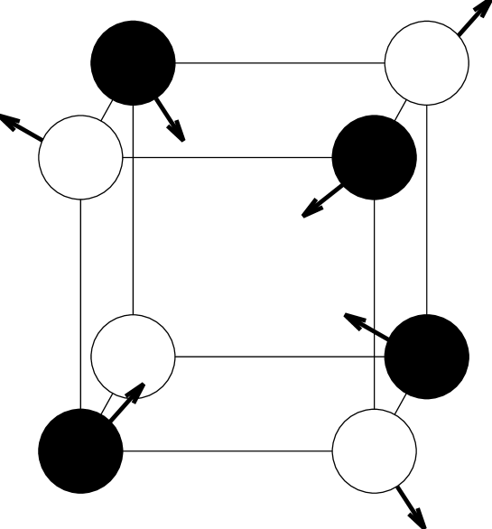
Figure 3: Schematic representation of 4-monopole scattering.

To make the above scattering process a little clearer we give a schematic representation in Fig 3. We draw a cube whose centre is at the origin and whose edges are parallel to the coordinate axes; it is to be associated with the cubic 4-monopole (compare Fig 2.). The incoming monopoles are represented by black spheres and the outgoing monopoles by white spheres, with an arrow indicating the direction of motion for each. Note that if one tried to extend this asymptotic interpretation to the region in which the monopoles are close together then one would conclude that the monopoles suffer no deflection and simply pass through each other. But this is misleading, since each of the outgoing monopoles cannot be identified with a single incoming monopole but is a composition of all the incoming ones. (A similar misleading interpretation exists for the scattering of three topological solitons in the plane. For $k$ solitons in the plane with cyclic $C_{k}$ symmetry the solitons scatter through an angle $\pi/k$, which for $k=3$ could mistakenly be taken for zero scattering angle).

To obtain a true picture of the scattering process, one needs to examine the energy density during the motion. Using our numerical scheme we can do this. Fig 4. shows a surface of constant energy density ${\cal E}=0.06$ for the five values $a=-0.25,-0.18,0.00,+0.18,+0.25$. We see that, indeed the energy density is initially localized in four regions roughly centered on the vertices of a tetrahedron. Let us think of these vertices as being opposite corners of a cube as in Fig 3. On any one face of the cube the incoming energy density is concentrated on two opposite corners of the face (black spheres in Fig 3.) and it flows around the edges of the face until it is localized on the two remaining corners (white spheres in Fig 3.) as the monopoles separate. This suggests that a useful way to view this scattering process is as pairs of $90^{\circ}$ scatterings occuring simultaneously.

5 Conclusion

Using a numerical scheme we have computed the energy densities of a 3-monopole with tetrahedral symmetry and a cubic 4-monopole with octahedral symmetry whose existence was recently proved [1]. We then proved the existence of a one parameter family of deformations of the cubic 4-monopole which has tetrahedral symmetry. In the moduli space approximation this describes a 4-monopole scattering process and we used our numerical scheme to analyse this further.

There are a number of interesting aspects which remain in the study of monopoles with the symmetries of regular solids. One obvious task is to construct a family of 3-monopole solutions which describes the scattering process in which the tetrahedral 3-monopole is formed. This problem is currently under investigation but is more difficult than the scattering considered in this paper, since the family has only $C_{3}$ symmetry which is not as useful as the tetrahedral symmetry which allowed us to solve the corresponding problem in the 4-monopole case. Another issue is that of a monopole with icosahedral symmetry. A monopole with icosahedral symmetry has to have charge at least six, but in [1] it was proved that no such monopole of charge six exists. We have proved that an icosahedral monopole of charge seven exists and are currently investigating its properties. These results and others on symmetric monopoles will be presented elsewhere [9].

Acknowledgements

Many thanks to Nigel Hitchin and Nick Manton for useful discussions. CJH thanks the EPSRC for a research studentship and the British Council for a FCO award. PMS thanks the EPSRC for a research fellowship.

Note added.

Recently the moduli space metric for the tetrahedrally symmetric 4-monopoles introduced in this paper has been calculated, P.M. Sutcliffe, Phys. Lett. 357B, 335 (1995).

References

• [1] N.J. Hitchin, N.S. Manton and M.K. Murray, Nonlinearity 8, 661 (1995).
• [2] N.S. Manton, Phys. Lett. 110B, 54 (1982).
D. Stuart, Commun. Math. Phys. 166, 149 (1994).
• [3] M.F. Atiyah and N.J. Hitchin, ‘The geometry and dynamics of magnetic monopoles’, Princeton University Press, 1988.
• [4] R.S. Ward, Commun. Math. Phys. 79, 317 (1981).
• [5] N.J. Hitchin, Commun. Math. Phys. 83, 579 (1982).
• [6] N.J. Hitchin, Commun. Math. Phys. 89, 145 (1983).
• [7] W. Nahm, ‘The construction of all self-dual multimonopoles by the ADHM method’, in Monopoles in quantum field theory, eds. N.S. Craigie, P. Goddard and W. Nahm, World Scientific, 1982.
• [8] F. Klein, ‘Lectures on the icosahedron’, London, Kegan Paul, 1913.
• [9] C.J. Houghton and P.M Sutcliffe, ‘Octahedral and Dodecahedral Monopoles’, to appear in Nonlinearity.