CPHT-RR013.0307

Orientifolds in ${\cal N}=2$ Liouville Theory and its Mirror

Dan Israël^♠ and Vasilis Niarchos^⋄

^♠ Racah Institute of Physics, The Hebrew University, Jerusalem 91904, Israel

greco, Institut d’Astrophysique de Paris, 98bis Bd Arago, 75014 Paris, France

^⋄Centre de Physique Théorique, Ecole Polytechnique, 91128 Palaiseau, France

Abstract

We consider unoriented strings in the supersymmetric SL(2,$\mathbb{R}$)/U(1) coset, which describes the two-dimensional Euclidean black hole, and its mirror dual $\mathcal{N}=2$ Liouville theory. We analyze the orientifolds of these theories from several complementary points of view: the parity symmetries of the worldsheet actions, descent from known AdS₃ parities, and the modular bootstrap method (in some cases we can also check our results against known constraints coming from the conformal bootstrap method). Our analysis extends previous work on orientifolds in Liouville theory, the AdS₃ and SU(2) WZW models and minimal models. Compared to these cases, we find that the orientifolds of the two dimensional Euclidean black hole exhibit new intriguing features. Our results are relevant for the study of orientifolds in the neighborhood of NS5-branes and for the engineering of four-dimensional chiral gauge theories and gauge theories with SO and Sp gauge groups with suitable configurations of D-branes and orientifolds. As an illustration, we discuss an example related to a configuration of D4-branes and O4-planes in the presence of two parallel fivebranes.

1 Introduction

Orientifolds play an important role in string theory (for a review see [1]). They appear in non-perturbative dualities and in many applications with clear phenomenological interest, especially since the advent of flux compactifications [2]. By nature, orientifolds are perturbative objects associated to the physics of unoriented strings that can be studied explicitly in perturbative string theory with the use of standard conformal field theory (cft) techniques. Their properties become richer in curved backgrounds where one has to face on the level of the worldsheet the complexities of a non-trivial cft. Related cft techniques were successfully applied to study Calabi-Yau compactifications at Gepner points in a series of papers [3, 4, 5, 6, 7, 8].

In this paper we want to study the orientifolds of two related theories: the ${\cal N}=2$ Liouville theory and the supersymmetric SL(2,$\mathbb{R}$)/U(1) coset. These theories are known to be dual [9, 10] and are mapped to each other by mirror symmetry [11]. From the cft point of view they are interesting as non-trivial (yet integrable) examples of irrational conformal field theories and provide a useful testing ground for ideas that may generalize to other irrational cfts. From the point of view of string theory, it is known that the supersymmetric coset SL(2,$\mathbb{R}$)/U(1) appears naturally as part of the worldsheet cft that describes string propagation in the vicinity of Calabi-Yau singularities [12, 13] and the near-horizon region of fivebranes in a double scaling limit [14, 15]. String theory in these situations is related holographically to a non-local, non-gravitational theory known as Little String Theory [16, 17, 18] and is in general non-critical.

Adding branes to this context gives another interesting application. It is well known that one can realize gauge theories with varying dimensionality and amount of supersymmetry in Hanany-Witten setups where one considers appropriate configurations of D-branes, orientifolds and NS5-branes (see [19, 20], the review [21] and references therein). Various non-trivial properties of gauge theories can be studied in this way. Certain Hanany-Witten setups can be studied directly in pertubative string theory by placing D-branes in the non-critical string theory of the previous paragraph, which involves, as we said, the SL(2,$\mathbb{R}$)/U(1) coset as part of its definition. D-branes in the ${\cal N}=2$ Liouville theory and the SL(2,$\mathbb{R}$)/U(1) coset have been constructed with cft methods in [22, 23, 24, 25, 26, 27] and will be summarized in sect. 2. This formalism was applied in the context of six-dimensional non-critical strings in [28] where it was shown explicitly how to realize four-dimensional ${\cal N}=1$ SQCD (see also [29]), and extended to models with supersymmetry breaking [30]. Further aspects of this theory (most notably Seiberg-duality) were analyzed in this context in [31].

Orientifolds in ${\cal N}=2$ Liouville theory and the supersymmetric SL(2,$\mathbb{R}$)/U(1) coset can be studied with similar cft methods. One can obtain important insights about these orientifolds from the corresponding analysis in bosonic Liouville theory [32], AdS₃ [33] and the non-supersymmetric and supersymmetric minimal models [34, 35, 36]. Orientifolds in ${\cal N}=2$ Liouville theory have been discussed previously in [37]. The results of that paper will be reproduced here with some important additions as a special case of our analysis.

In order to set up our notation and to gather certain facts for later use, we devote section 2 to a brief review of open and closed strings in AdS₃, SL(2,$\mathbb{R}$)/U(1) and ${\cal N}=2$ Liouville theory. Sections 3, 4 and 5 discuss different classes of orientifolds in the ${\cal N}=2$ Liouville theory and the supersymmetric SL(2,$\mathbb{R}$)/U(1) coset and contain the main results of this paper.

In this work, we use three different approaches to uncover information about orientifolds: the explicit form of the allowed symmetries that can be combined with worldsheet parity, descent of known AdS₃ parities to SL(2,$\mathbb{R}$)/U(1) and a direct modular bootstrap approach (in some cases, we can also check our results against known conformal bootstrap constraints). Each approach has its merits and its disadvantages, but comparison of the information obtained in this way yields important checks and helps complete the picture.

In sect. 3 we classify a set of consistent worldsheet parities. This is most straightforward in the ${\cal N}=2$ Liouville theory because of the simplicity of the worldsheet action. This approach gives naturally ${\rm O2}$- and ${\rm O}1$-planes that extend towards the weak coupling region of the theory. One of the interesting results of this analysis is a parity that can be used to construct non-critical, non-tachyonic type $0^{\prime}$B string vacua. The explicit construction of these vacua will appear in a companion paper [38]. We also analyze parities that descend from AdS₃. This point of view gives a natural set of orientifolds with the geometry of ${\rm O0}$-, ${\rm O1}$- and ${\rm O2}$-planes on SL(2,$\mathbb{R}$)/U(1) .

In sect. 4 we proceed to analyze with exact cft methods the crosscap wave-functions of two B-type parities on SL(2,$\mathbb{R}$)/U(1) . The exact result reproduces the semiclassical asymptotic Klein bottle amplitude based on the known action of the parities, but also reveals the presence of an additional localized orientifold contribution. We propose that the latter corresponds to one of the ${\rm O0}$-planes that was found in sect. 3. Hence, we find that the cft gives naturally not a single ${\rm O0}$- or an ${\rm O2}$-plane, but a specific combination of the two. We provide a physical interpretation of this result in the context of Hanany-Witten setups.

In the final section, we discuss the crosscap wave-function of an A-type orientifold that gives an ${\rm O}1$-plane on SL(2,$\mathbb{R}$)/U(1) . We obtain this result by descent from an Euclidean AdS₂ orientifold in Euclidean AdS₃. The AdS₂ orientifold can be obtained from an H₂ orientifold with an SL(2,$\mathbb{C}$) rotation. This provides and independent derivation of the AdS₂ crosscap wavefunction in [33].

Three appendices supplement the material of the main text. In the first two appendices we summarize some of our conventions and list the known D-brane wave-functions for quick reference. In the third appendix we derive the ${\cal P}$-modular transformation properties of the identity character which will be instrumental in the modular bootstrap approach of sect. 4. The derivation appearing in appendix C is a generalization of the one appearing in [37] but with some important differences.

Note added. We are aware that Sujay Ashok, Sameer Murthy and Jan Troost have been exploring independently a related subject.

2 Strings and branes in SL(2,$\mathbb{R}$)/U(1) & ${\cal N}=2$ Liouville

We start with a brief review of the SL(2,$\mathbb{R}$)/U(1) conformal field theory and its mirror ${\cal N}=2$ Liouville theory. This will help us set up our conventions and gather some important facts for later use. For more details on the material reviewed in this section we refer the reader to the original references cited below.

Closed strings in AdS₃

String theory on AdS₃ [40] with an ns-ns two-form flux is an exact solution of string theory, whose background fields read, in global coordinates

$$\text{d}s^{2}=\alpha^{\prime}k\left[\text{d}\rho^{2}+\sinh^{2}\rho\,\text{d}\phi^{2}-\cosh^{2}\rho\,\text{d}t^{2}\right],\quad H=2\alpha^{\prime}k\cosh\rho\sinh\rho\ \text{d}\rho\wedge\text{d}\phi\wedge\text{d}t\,$$ (2.1)

with a constant dilaton. The global SO(2,2) symmetry of this space-time is enhanced to an affine $\widehat{\mathfrak{sl}}(2,\mathbb{R})_{\textsc{l}}\times\widehat{\mathfrak{sl}}(2,\mathbb{R})_{\textsc{r}}$ since we can take the worldsheet theory as the wzw model for the group SL(2,$\mathbb{R}$) . To be more precise, AdS₃ space-time with a non-compact global time $t$ corresponds to the universal cover of SL(2,$\mathbb{R}$) . In order to obtain superstring backgrounds, one can define the super-wzw model for SL(2,$\mathbb{R}$) by adding three free worldsheet fermions of signature $(-,+,+)$. The central charge of this $\mathcal{N}=1$ superconformal theory is $c=9/2+6/k$.

Primary states of the model are classified in terms of $\widehat{\mathfrak{sl}}(2,\mathbb{R})$ representations, that can be twisted by an outer automorphism called spectral flow [41, 42]. Their conformal weights read, in the ns-ns sector:

$$\Delta_{\mathfrak{sl}}=-\frac{j(j-1)}{k}-wm+\frac{kw^{2}}{4}\quad,\qquad\bar{\Delta}_{\mathfrak{sl}}=-\frac{j(j-1)}{k}-w\bar{m}+\frac{kw^{2}}{4}~{},$$ (2.2)

where $(m,\bar{m})$ label the primaries of the elliptic sub-algebra $(J^{3},\bar{J}^{3})$ and $w$ is the spectral flow parameter. Space-time energy is given by $E=m+\bar{m}$ whereas the angular momentum (conjugate to $\phi$) is $n=m-\bar{m}\in\mathbb{Z}$. The unitary closed string spectrum is made of continuous representations with $j\in\nicefrac{{1}}{{2}}+i\mathbb{R}_{+}$ and discrete representations in the range $\nicefrac{{1}}{{2}}<j<\nicefrac{{k+1}}{{2}}$. We refer the reader to appendix A for more details about these representations.

Closed strings in SL(2,$\mathbb{R}$)/U(1)

The SL(2,$\mathbb{R}$)/U(1) conformal field theory [43, 44, 45, 46] is obtained from SL(2,$\mathbb{R}$) as a gauged wzw model. One possibility is to perform an axial gauging of the elliptic subalgebra, corresponding to the time-translation symmetry $t\to t+\lambda_{\text{a}}$. This symmetry has no fixed point, hence the background is non-singular

$$\text{d}s^{2}=\alpha^{\prime}k\left[\text{d}\rho^{2}+\tanh^{2}\rho\,\text{d}\phi^{2}\right]\ ,\quad\Phi=\Phi_{0}-2\ln\cosh\rho\,,$$ (2.3)

and has the interpretation of a two-dimensional Euclidean black hole, the cigar. Using the standard gauging construction, the primary states of the coset can be obtained from SL(2,$\mathbb{R}$) primaries with $m+\bar{m}=0$, with conformal weights (for ns-ns primaries)

$$\Delta_{\mathfrak{cig}} =\Delta_{\mathfrak{sl}}+\frac{m^{2}}{k}=-\frac{j(j-1)}{k}+\frac{(n+kw)^{2}}{4k}$$ (2.4a)

$$\bar{\Delta}_{\mathfrak{cig}} =\bar{\Delta}_{\mathfrak{sl}}+\frac{\bar{m}^{2}}{k}=-\frac{j(j-1)}{k}+\frac{(n-kw)^{2}}{4k}$$ (2.4b)

The periodicity $\phi\sim\phi+2\pi$ of AdS₃, see eqn. (2.1), is inherited by the coset. At the asymptotic $\rho\rightarrow\infty$ region, $\phi$ becomes a canonically normalized free boson at radius $\sqrt{\alpha^{\prime}k}$. One identifies $n$ as the momentum of this boson, and $w$ as its winding number. Correlators of this theory can be computed by descent from the corresponding quantities in H${}_{3}^{+}$ [47, 48].

The leading order solution of the background fields (2.3) is exact to all orders in $\nicefrac{{1}}{{k}}$ as the superconformal symmetry is enlarged to $\mathcal{N}=2$ [49, 50]. However it receives non-perturbative corrections in the form of a ”winding condensate” [9, 10, 11, 51, 52]. In the asymptotic region $\rho\to\infty$ where the fields $\rho$, $\phi$ and their fermionic superparters $\psi^{\pm}=\psi^{\rho}\pm i\psi^{\phi}$ are free one can write the winding condensate as a worldsheet interaction of the form

$$\delta S=\frac{k}{2\pi}\int\text{d}^{2}z\,e^{-k\rho}\left[i\mu\,\psi^{+}\bar{\psi}^{-}e^{ik(\phi_{L}-\phi_{R})}+i\mu^{\dagger}\,\psi^{-}\bar{\psi}^{+}e^{-ik(\phi_{L}-\phi_{R})}\right]\,.$$ (2.5)

Another consistent theory is defined by a vector gauging that refers to the symmetry $\phi\to\phi+\lambda_{\text{v}}$ and gives the constraint $m-\bar{m}=0$. Since $\rho=0$ is a fixed point of this isometry, the leading order metric $\text{d}s^{2}=\alpha^{\prime}k[\text{d}\rho^{2}+\text{cotanh}^{2}\,\rho\,\text{d}\tilde{\phi}^{2}]$ is a singular geometry known as the trumpet. As the geometric interpretation breaks down it is usually more appropriate to view this model as an $\mathcal{N}=2$ Liouville theory [10, 11, 51], defined as a free $\mathcal{N}=2$ linear dilaton theory perturbed by a momentum condensate T-dual to (2.5), i.e. with $\phi_{L}-\phi_{R}$ replaced by $\tilde{\phi}$ (and $\bar{\psi}^{\pm}$ by $\bar{\psi}^{\mp}$). We will discuss this model in more detail below.

Contrary to the axial gauging, the vectorially gauged SL(2,$\mathbb{R}$)/U(1) coset is sensitive to the cover of SL(2,$\mathbb{R}$) [53]. Starting with the universal cover of AdS₃ we obtain a non-compact coordinate $\tilde{\phi}$ – this coordinate is the time coordinate $t$ in disguise. Starting with the single cover, the field $\tilde{\phi}$ corresponds in the asymptotic region $\rho\to\infty$ to a free boson at radius $\sqrt{\alpha^{\prime}k}$. This defines a consistent cft at the non-perturbative level only if the level $k$ is an integer, otherwise the momentum condensate dual to (2.5) is not periodic. For irrational $k$, the only consistent theory with a momentum condensate and finite radius is obtained with T-duality from the cigar (2.3); in that case the radius of the transverse coordinate is $\sqrt{\alpha^{\prime}/k}$. This model cannot be obtained as a gauging of AdS₃; however, for integer $k$ it is the $\mathbb{Z}_{k}$ orbifold of the trumpet at radius $\sqrt{\alpha^{\prime}k}$. We summarize the various possibilities in table 1. The last two rows correspond to the same models, provided the radii are equal.

	k integer	k arbitrary
Axial gauging	$R=\sqrt{\alpha^{\prime}k}$	$R=\sqrt{\alpha^{\prime}k}$
Vector gauging	$R=\infty$ or $R=\sqrt{\alpha^{\prime}k}$	$R=\infty$
$\mathcal{N}=2$ Liouville	$R=\infty$, $R=\sqrt{\alpha^{\prime}k}$ or $R=\sqrt{\alpha^{\prime}/k}$	$R=\infty$, $R=\sqrt{\alpha^{\prime}/k}$

Table 1: Various SL(2,$\mathbb{R}$)/U(1) theories

D-branes and boundary cft

Various D-branes have been constructed, using the tools of boundary conformal field theory, in H${}_{3}^{+}$ [54, 55] and later in Lorentzian AdS₃ [56]. They are classified by the gluing conditions imposed on the $\widehat{\mathfrak{sl}}(2,\mathbb{R})$ currents [57]. Extending the coset construction to bcft, corresponding branes have been obtained in SL(2,$\mathbb{R}$)/U(1) [22, 23]. These results are mainly in agreement with other approaches, such as modular bootstrap [24, 25, 26] and conformal bootstrap based on the $\mathcal{N}=2$ superconformal algebra [27]. In what follows we summarize the branes that will be most interesting for the analysis below. The corresponding wave-functions, i.e. the coefficient of the one-point functions on the disc, are summarized in app. B.

D0-branes

The D(-1)-brane (i.e. point-like in space-time) of AdS₃ can be obtained with the current algebra gluing conditions $J^{3}=-\bar{J}^{3}|_{z=\bar{z}}$, $J^{\pm}=-\bar{J}^{\mp}|_{z=\bar{z}}$ using the conventions of [55]. Its main property is that the spectrum of open strings attached to it contains only the identity representation of $\widehat{\mathfrak{sl}}(2,\mathbb{R})$. It is located at $\rho=0$ and $t=0,\pi$ on the single cover, i.e. the brane is made of two copies. D0-branes in the coset SL(2,$\mathbb{R}$)/U(1) can be obtained from the D(-1)-brane of AdS₃ by descend. Corresponding D0-branes in ${\cal N}=2$ Liouville theory exist by mirror symmetry.

Let us consider first the D0-brane of non-compact $\mathcal{N}=2$ Liouville theory, or non-compact ”trumpet” background. In the $\mathcal{N}=2$ terminology this is an A-type brane. The quantization of the brane position at $\tilde{\phi}=2\pi r/k$ with $r\in\mathbb{Z}$ has its origin in the $\mathcal{N}=2$ Liouville potential that breaks the translation symmetry along $\tilde{\phi}$ to a $\mathbb{Z}$ subgroup generated by $\tilde{\phi}\to\tilde{\phi}+2\pi/k$. It is quite analogous to the ”special points” at the boundary of the disc in SU(2)/U(1) [58]. Using the conventions of app. A, we can write the annulus amplitude in this theory (in the ns sector), for open strings stretched between D0-branes sitting at $\phi=2\pi r/k$ and $2\pi r^{\prime}/k$, as:

$$\mathcal{A}_{r\,r^{\prime}}(t)=ch_{\mathbb{I}}(r^{\prime}-r;it){0\atopwithdelims[ ]0}\,.$$ (2.6)

It contains only one identity character of the $\mathcal{N}=2$ superconformal algebra.

The cigar cft (T-dual to the minimal radius $\mathcal{N}=2$ Liouville theory) is obtained by modding out the $\mathbb{Z}$ subgroup of the translation symmetry that is not broken non-perturbatively. Since this symmetry has no fixed point one can obtain the boundary state by summing over the images under the orbifold action. As a result, the brane carries no label (apart from the usual labels characterizing the fermionic boundary conditions). It is a D0-brane localized at the tip $\rho=0$ with B-type boundary conditions. One obtains the annulus amplitude by summing (2.6) over $r\in\mathbb{Z}$. The closed string one-point functions on the disc in all fermionic sectors are summarized in app. B.

Finally, for integer $k$ one can consider the trumpet at radius $\sqrt{\alpha^{\prime}k}$, the vector gauging of the single cover. In this case, one mods out the non-compact model by the subgroup $\tilde{\phi}\to\tilde{\phi}+2\pi$. The annulus amplitude for the D0-brane is obtained from a partial summation of (2.6) as $r=\hat{r}+k\mathbb{Z}$. One can repackage the result using the extended characters defined in app. A. The result in the ns-ns sector is

$$\mathcal{A}^{\mathrm{vect.\,}}_{\hat{r}\,\hat{r}^{\prime}}(t)=Ch_{\mathbb{I}}(\hat{r}^{\prime}-\hat{r};it){0\atopwithdelims[ ]0}\,.$$ (2.7)

Summing over $\hat{r}\in\mathbb{Z}_{k}$ gives the annulus amplitude for the cigar written with extended characters.

D1-branes

The D1-branes of the two-dimensional black hole descend from the AdS₂ branes of AdS₃ [57]. They are characterized by A-type boundary conditions of the $\mathcal{N}=2$ superconformal algebra (sca). Their embedding equation is

$$\sinh\rho\,\sinh(\phi-\hat{\phi})=\sinh\hat{\rho}$$ (2.8)

with two continuous parameters $(\hat{\rho},\hat{\phi})$. In the asymptotic cylinder region, these branes have the shape of two antipodal D1-branes at $\phi=\hat{\phi},\ \hat{\phi}+\pi$. The open string spectrum comprises only of continuous representations, with a non-trivial density of states [22, 23] associated with the

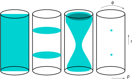
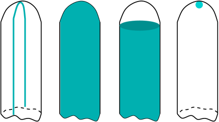
Figure 1: Geometries of various D-branes on the single cover of AdS₃ (upper picture) and in the cigar (lower picture). From left to right: AdS₂ brane with $\hat{\rho}=0$, H₂ branes with $\hat{\sigma}=0$, dS₂ brane and D(-1)-branes. Roughly speaking, the cigar coset is obtained by projecting onto an ”horizontal slice” of the cylinder and the trumpet onto a ”vertical slice”.

boundary two-point function. The relevant one-point function on the disc is given by eqn. (B.4). In the non-compact trumpet / $\mathcal{N}=2$ Liouville theory, one obtains a D2-brane with a worldvolume $\rho>\hat{\rho}$ endowed with a magnetic field.

D2-branes

Finally, one can define space-like branes in AdS₃ with H₂ geometry. In H${}_{3}^{+}$ these branes are equivalent to AdS₂ branes by SL(2,$\mathbb{C}$) rotation. By descent they give D2-branes on the cigar, with B-type boundary conditions, carrying a magnetic field [22]. The latter is quantized because the brane carries a D0-brane charge near the tip of the cigar. In the non-compact trumpet / $\mathcal{N}=2$ Liouville theory, the AdS₂ branes give D1-branes with embedding equation $\sinh\rho\sin(\tilde{\phi}-\hat{\varphi})=\sin\hat{\sigma}$. In this case, the quantization of $\hat{\sigma}$ is interpreted as the requirement that the brane ends on one of the special points at $\rho=0$ [59] (the parameter $\hat{\varphi}$ is also quantized). However, these branes seem to be inconsistent for irrational $k$ since their open string spectrum contains negative multilplicities [23]. A different class of D2-branes, related to dS₂ geometries in Lorentzian AdS₃ (this class of branes cannot descend from branes in H${}_{3}^{+}$), have been constructed using modular bootstrap methods in [26] and conformal bootstrap methods in ${\cal N}=2$ Liouville theory in [27] (for a dbi analysis of these branes see [60]). D2-branes in this class are free of the abovementioned problems since their open string spectrum is made of continuous representations only. They exhibit a double-sheeted structure that covers the domain $\rho>\rho_{\text{min}}$ and are labeled by a continuous parameter that characterizes the minimal distance $\rho_{\text{min}}$ from the tip of the cigar and a $\mathbb{Z}_{2}$-valued Wilson line. Their boundary state wave-functions are summarized in app. B. It should be pointed out that these D2-branes are related to D2-branes of the first category with an overcritical magnetic field [60].

We sketch the brane geometries in fig. 1. Note that other types of branes, whose geometrical and physical interpretation has not yet been elucidated, were considered in [61, 62].

3 Parities and the geometry of orientifolds

In this section we discuss the orientifolds of the supersymmetric SL(2,$\mathbb{R}$)/U(1) coset and the ${\cal N}=2$ Liouville theory from the perspective of the parity symmetries. This point of view allows for a first look at the semiclassical features of the orientifolds and provides a useful guide for the exact analysis of the next section. First, we classify a set of A- and B-type parities in $\mathcal{N}=2$ Liouville theory. Then we repeat the exercise with parities in SL(2,$\mathbb{R}$)/U(1) inherited from AdS₃. The simultaneous analysis of parity symmetries in both theories is useful, because certain orientifolds are easier to analyze in one theory than the other. Of course, at the end of the day the orientifolds of these theories are related by mirror symmetry. We comment on this correspondence at the end of this section.

Parities in worldsheet theories with ${\cal N}=(2,2)$ supersymmetry

In a two-dimensional qft with ${\cal N}=(2,2)$ supersymmetry one can define a natural set of parity symmetries (we recommend [36] for an excellent discussion of the general situation). Here it will be useful to highlight the main points of these symmetries. The two bosonic coordinates of the ${\cal N}=(2,2)$ superspace will be denoted as $(z,\bar{z})$ and the four fermionic coordinates as $\theta,\bar{\theta}$ and $\theta^{\dagger},\bar{\theta}^{\dagger}$. As above, we denote the right-movers with a bar and reserve the dagger for the notation of complex conjugate quantities. The ${\cal N}=2$ superconformal algebra generators will be denoted as $T(z),J(z),G^{\pm}(z)$ for the left-movers with an analogous notation for the right-movers.

There are two basic parities in a theory with ${\cal N}=(2,2)$ supersymmetry that reverse the worldsheet chirality (exchanging the left- and right-movers) while preserving the holomorphy of the ${\cal N}=2$ supersymmetry. They are known as A- and B-type and are defined by the worldsheet action

$$\Omega_{A}~{}: \quad(z,\bar{z},\theta,\bar{\theta},\theta^{\dagger},\bar{\theta}^{\dagger})\rightarrow(\bar{z},z,-\bar{\theta}^{\dagger},-\theta^{\dagger},-\bar{\theta},-\theta)~{},$$ (3.1a)

$$\Omega_{B}~{}: \quad(z,\bar{z},\theta,\bar{\theta},\theta^{\dagger},\bar{\theta}^{\dagger})\rightarrow(\bar{z},z,\bar{\theta},\theta,\bar{\theta}^{\dagger},\theta^{\dagger})~{}.$$ (3.1b)

They act on the supercurrents as

$$\Omega_{A}~{}: \quad G^{\pm}(z)\rightarrow\bar{G}^{\mp}(\bar{z})~{},~{}~{}\qquad\qquad\Omega_{A}~{}:\quad\bar{G}^{\pm}(\bar{z})\rightarrow G^{\mp}(z)~{},$$ (3.2a)

$$\Omega_{B}~{}: \quad G^{\pm}(z)\rightarrow\bar{G}^{\pm}(\bar{z})~{},~{}~{}\qquad\qquad\Omega_{B}~{}:\quad\bar{G}^{\pm}(\bar{z})\rightarrow G^{\pm}(z)$$ (3.2b)

and on the R-symmetry currents as

$$\Omega_{A}~{}: \quad J(z)\rightarrow-\bar{J}(\bar{z})~{},~{}~{}\qquad\qquad\Omega_{A}~{}:\quad\bar{J}(\bar{z})\rightarrow-J(z)~{},$$ (3.3a)

$$\Omega_{B}~{}: \quad J(z)\rightarrow\phantom{-}\bar{J}(\bar{z})~{},~{}~{}\qquad\qquad\Omega_{B}~{}:\quad\bar{J}(\bar{z})\rightarrow J(z)~{}.$$ (3.3b)

The two parities are exchanged by mirror symmetry. The same thing happens with boundary conditions, where mirror symmetry exchanges A- and B-type branes.

One can generalize the above parities by combining them with internal discrete symmetries $\tau$ of the theory (we will present explicit examples of such symmetries in ${\cal N}=2$ Liouville theory and its mirror dual below). In this way one can formulate more general A- and B-type parities of the form

$${\cal P}_{A}=\tau_{A}\cdot\Omega_{A}~{},~{}~{}{\cal P}_{B}=\tau_{B}\cdot\Omega_{B}$$ (3.4)

which are still acting on the supercurrents as in (3.2a, 3.2b) and on the R-symmetry currents as in (3.3a, 3.3b) provided, of course, that the internal symmetries preserve the $R$-symmetry currents. A general example of such A- and B-type parities are the $(\alpha,\beta)$ parities

$${\cal P}_{A_{\alpha,\beta}}=e^{-i\alpha J-i\beta\bar{J}}\cdot\Omega_{A}~{},~{}~{}{\cal P}_{B_{\alpha,\beta}}=e^{-i\alpha J-i\beta\bar{J}}\cdot\Omega_{B}~{},$$ (3.5)

where one combines the basic worldsheet parities $\Omega_{A}$, $\Omega_{B}$ with $U(1)_{R}$ rotations. It should be pointed out that for general values of $\alpha$ and $\beta$ these parities are not involutive (i.e. ${\cal P}^{2}\neq 1$). Also they are non-geometric, because they treat the left- and right-movers asymmetrically. The latter can have interesting consequences for the resulting theory; we will mention an interesting example below.

Parities in ${\cal N}=2$ Liouville theory

We are now in position to examine the A- and B-type parity symmetries of the ${\cal N}=2$ Liouville action (we set $\alpha^{\prime}=2$)

$$S=\frac{1}{8\pi}\int\text{d}^{2}z\,\text{d}^{4}\theta\,\Phi\bar{\Phi}+\frac{\mu}{2\pi}\int\text{d}^{2}z\,\text{d}\theta\text{d}\bar{\theta}\,e^{-\sqrt{\frac{k}{2}}\Phi}+\frac{\mu^{\dagger}}{2\pi}\int\text{d}^{2}z\,\text{d}\theta^{\dagger}\text{d}\bar{\theta}^{\dagger}\,e^{-\sqrt{\frac{k}{2}}\bar{\Phi}}$$ (3.6)

written in terms of a chiral $\mathcal{N}=2$ superfield

$$\Phi=r+i\varphi+i\sqrt{2}\theta\psi^{+}+i\sqrt{2}\bar{\theta}\bar{\psi}^{+}+2\theta\bar{\theta}F+\cdots$$ (3.7)

$r$ denotes the radial direction and $\varphi$ the angular direction. This theory is superconformal provided the background charge satisfies $Q=\sqrt{2/k}$. In the asymptotic $r\to\infty$ weakly coupled region, the left and right $U(1)_{R}$ currents read, in terms of the component fields:

$$J =\psi^{+}\psi^{-}+iQ\partial\varphi$$ (3.8a)

$$\bar{J} =\bar{\psi}^{+}\bar{\psi}^{-}+iQ\bar{\partial}\varphi$$ (3.8b)

The potential coming from the superfield action (3.6) is similar to the interaction term (2.5) after the change of normalization of the fields $(\rho,\phi)=(2k)^{-\nicefrac{{1}}{{2}}}(r,\varphi)$ and T-duality. In this alternate description of the SL(2,$\mathbb{R}$)/U(1) theory, the first term in the asymptotic expansion of the cigar geometry, eqn. (2.3), comes as a a correction to the Kähler potential (3.6)

$$\delta S=\mu_{\text{cig}}\int\text{d}^{2}z\,\text{d}^{4}\theta\ e^{-\frac{\Phi+\Phi^{\dagger}}{\sqrt{2k}}}~{}.$$ (3.9)

The basic A- and B-type parities $\Omega_{A}$ and $\Omega_{B}$ leave the fermionic measure $d\theta d\bar{\theta}d\theta^{\dagger}d\bar{\theta}^{\dagger}$ invariant and act on the ${\cal N}=2$ Liouville chiral superfield $\Phi$ as

$$\Omega_{A}~{}:~{}\Phi(z,\bar{z},\theta,\bar{\theta})\rightarrow\left\{\Phi(\Omega_{A}(z,\bar{z},\theta,\bar{\theta}))\right\}^{\dagger}~{},~{}~{}\Omega_{B}~{}:~{}\Phi(z,\bar{z},\theta,\bar{\theta})\rightarrow\Phi(\Omega_{B}(z,\bar{z},\theta,\bar{\theta}))~{}.$$ (3.10)

Hence, if we write the ${\cal N}=2$ Liouville action (3.6) as

$$S=S_{\text{K\"{a}hler}}+S_{\text{Liouville}}(\mu)+S^{\dagger}_{\text{Liouville}}(\mu^{\dagger})$$ (3.11)

we can easily verify that the Kähler (kinetic) part of the action is invariant under both $\Omega_{A}$ and $\Omega_{B}$, but the superpotential parts are transforming as

$$\Omega_{A}~{}:~{}S_{\text{Liouville}}(\mu)\rightarrow S_{\text{Liouville}}(\mu)^{\dagger}~{},$$ (3.12)

$$\Omega_{B}~{}:~{}S_{\text{Liouville}}(\mu)\rightarrow S_{\text{Liouville}}(-\mu)~{}.$$ (3.13)

Consequently, $\Omega_{A}$ is a true symmetry of the ${\cal N}=2$ Liouville theory only when $\mu\in\mathbb{R}$. On the other hand, $\Omega_{B}$ cannot be a true symmetry unless we take $\mu=0$, i.e. unless we drop the ${\cal N}=2$ Liouville interaction term to be left with a free linear dilaton theory.

The ${\cal N}=2$ Liouville theory has two obvious involutive parities that can be used to define B-type orientifolds. These are a parity $s$ that shifts the angular coordinate $\varphi$ by half a period, i.e.

$$s~{}:\quad\varphi\rightarrow\varphi+\pi Q~{}$$ (3.14)

and the fermionic parity $(-)^{\bar{F}}$ where $\bar{F}$ is the right-moving worldsheet fermion number. Under the parities ${\cal P}_{B}=s\cdot\Omega_{B}$ and ${\cal P}^{\prime}_{B}=(-)^{\bar{F}}\cdot\Omega_{B}$ the full ${\cal N}=2$ Liouville action is invariant. $(-)^{\bar{F}}$ can also be combined with $\Omega_{A}$ to give a consistent A-type parity.

Given the above symmetries of the classical $\mathcal{N}=2$ Liouville theory

$${\cal P}_{A}=\Omega_{A}~{},~{}~{}{\cal P}^{\prime}_{A}=(-)^{\bar{F}}\cdot\Omega_{A}~{},~{}~{}{\cal P}_{B}=s\cdot\Omega_{B}~{},~{}~{}{\cal P}^{\prime}_{B}=(-)^{\bar{F}}\cdot\Omega_{B}$$ (3.15)

we can define the corresponding $(\alpha,\beta)$ $U(1)_{R}$ rotated versions as

$${\cal P}_{A_{\alpha,\beta}}=\Omega_{A_{\alpha,\beta}}~{},~{}~{}{\cal P}_{A_{\alpha,\beta}}=(-)^{\bar{F}}\cdot\Omega_{A_{\alpha,\beta}}~{},~{}~{}{\cal P}_{B_{\alpha,\beta}}=s\cdot\Omega_{B_{\alpha,\beta}}~{},~{}~{}{\cal P}_{B_{\alpha,\beta}}=(-)^{\bar{F}}\cdot\Omega_{B_{\alpha,\beta}}~{}.$$ (3.16)

For general $\alpha$ and $\beta$ these parities are non-involutive.

The non-perturbative consistency of these parities requires that they leave invariant the cigar interaction (3.9). One can check that this requirement is trivially satisfied by all of the above parities.

In the context of type 0 non-critical strings the parity ${\cal P}_{B_{0,0}}$, as well as ${\cal P}^{\prime}_{B_{0,\pi}}$, leads to an interesting theory of non-oriented type 0 strings without closed string tachyons, no fermions and no massless tadpoles, which is a cousin of the type $0^{\prime}$B theory in ten dimensions. In the context of two dimensional type 0 strings based on ${\cal N}=1$ Liouville theory it was pointed out in [63, 64] that the type $0^{\prime}$B projection is not allowed, because it projects out the ${\cal N}=1$ Liouville interaction. In ${\cal N}=2$ Liouville theory we see, however, that this is no longer the case and the type $0^{\prime}$B projection is indeed possible. A detailed analysis of this theory will appear elsewere [38].

Geometric parities in AdS₃ and its cosets

In this subsection we take an orthogonal route to look at the possible geometric parities in the axial SL(2,$\mathbb{R}$)/U(1) coset, i.e. the cigar geometry given by eqn. (2.3). For the moment, let us forget about the details of the worldsheet fermions and supersymmetry and look first at the parity symmetries of the bosonic SL(2,$\mathbb{R}$) WZW model, following [65]. Possible orientifold projections combine the worldsheet orientation symmetry and a $\mathbb{Z}_{2}$ isometry. The isometries of the manifold are most easily described by embedding AdS₃ in $\mathbb{R}^{2,2}$ with the equation:

$$(X^{0})^{2}+(X^{3})^{2}-(X^{1})^{2}-(X^{2})^{2}=\alpha^{\prime}k\,.$$ (3.17)

We will consider geometric $\mathbb{Z}_{2}$ symmetries that are combinations of the parities $X^{i}\to-X^{i}$ for $i=1,\ldots 4$. The global coordinates on the group manifold, see the metric (2.1), are defined as

$$X^{0}\pm iX^{3}=\sqrt{\alpha^{\prime}k}\cosh\rho\ e^{\pm it}\quad,\qquad X^{1}\pm iX^{2}=\sqrt{\alpha^{\prime}k}\sinh\rho\ e^{\pm i\phi}\,.$$ (3.18)

In the wzw model the parity symmetry has to reverse the orientation of the target space manifold in order to preserve the Wess-Zumino term $\int(g^{-1}\text{d}g)^{\wedge 3}$, i.e. the coupling to the ns-ns two-form. In view of the applications to the coset we don’t restrict ourselves to parities with an invariant timelike hypersurface. We give the various inequivalent choices ($i.e.$ which are not related one the the other by the isometries of the manifold) for the orientifold geometry in table 2.

$$\begin{array}[]{|c|l|l|l|}\hline\cr\text{}&\text{Action in }\mathbb{R}^{2,2}&\text{AdS${}_{3}$ global coordinates}&\text{Fixed submanifold}\\ \hline\cr\tau_{1}&X^{2}\to-X^{2}&\phi\to-\phi&\phi=0,\pi\ (\text{AdS}_{2})\\ \tau_{2}&X^{3}\to-X^{3}&t\to-t&t=0\ (\text{H}_{2})\\ \tau_{3}&X^{1}\to-X^{1}\,,\ X^{2}\to-X^{2}\,,\ X^{3}\to-X^{3}&t\to-t\,,\ \phi\to\phi+\pi&\rho=t=0\ (\text{point})\\ \tau_{4}&X^{0}\to-X^{0}\,,\ X^{2}\to-X^{2}\,,\ X^{3}\to-X^{3}&t\to t+\pi\ ,\ \phi\to-\phi&\text{none}\\ \hline\cr\end{array}$$

Table 2: Geometric parities in the AdS₃ wzw model

In the last case the orientifold action has no fixed submanifold. It is an involution only on the single cover of the group manifold, for which $t\sim t+2\pi$.

Let us also define other parities that do not show up in the above analysis since they are not strictly speaking geometric. It is well known in a free U(1) theory parametrized by a boson $t$ that the parity $t\to-t$ can be performed together with a winding shift, i.e. a one-half translation of the coordinate T-dual to $t$ [35]. We can consider a similar modification of the $\tau_{2}$ parity, provided we start with the single cover of AdS₃. It defines a parity $\tilde{\tau}_{2}$. Geometrically, instead of a pair of H₂ orientifold planes at $t=0$ and $t=\pi$ with the same tension, we get a pair of orientifolds with opposite tension. Similarly, one can define a $\tilde{\tau}_{3}$ parity corresponding to a pair of O(-1) planes of opposite tension.

Let us consider now the axial coset SL(2,$\mathbb{R}$)/U(1) , i.e. the cigar, and analyze how the above-mentioned parities are realized. The six AdS₃ parities give orientifold planes with the following geometries:

• For $\tau_{1}$ the geometry is similar to that of a straight D1-brane with $\hat{\rho}=0$, which is localized at $\phi=0,\pi$, see lower-left picture in fig. 1.

• For $\tau_{2}$ the ${\rm O}$-plane covers all the cigar, similar to a D2-brane with $\hat{\sigma}=0$.

• For $\tau_{3}$ the geometry is similar to that of the D0-brane of the cigar, i.e. it is localized at $\rho=0$.

• For $\tau_{4}$ we obtain something similar to the O1-plane above, but with an extra winding shift $\phi_{L}-\phi_{R}\to\phi_{L}-\phi_{R}+\pi$.

• For $\tilde{\tau}_{2}$ we obtain again a geometry that resembles that of a D2-brane with $\hat{\sigma}=0$, however the parity acts with an extra one-half rotation along the transverse direction $\phi$.

• For $\tilde{\tau}_{3}$ the geometry is similar to that of $\tau_{3}$.

The parity $\tau_{4}$ is identified in the cigar with the combination of the inversion $\phi\to-\phi$ and a winding shift by realizing that the translation symmetry along $t$, which amounts to the translation symmetry in the vector coset (i.e. the trumpet) becomes the winding symmetry in the axial coset. However, we know that this symmetry is broken at the non-perturbative level by the winding condensate (2.5). Hence, we conclude that this parity is not consistent in SL(2,$\mathbb{R}$)/U(1) . All other parities leave the winding condensate invariant, in agreement with the analysis done in ${\cal N}=2$ Liouville as we will see in the next paragraph.

In the vector coset, or ${\cal N}=2$ Liouville theory, the parities $\tau_{1}$ and $\tau_{3}$ give respectively an O2-plane and a localized A-type orientifold whose geometrical nature is not well-defined. The parity $\tau_{2}$ gives a pair of antipodal O1-planes of the same tension. On the single cover of the trumpet, one can define a parity $\tilde{\tau}_{2}$ as we saw above, which includes a winding shift. It gives a pair of antipodal O1-planes of opposite tension. On the universal cover there is of course no such parity, or better saying it cannot be distinguished from the parity $\tau_{2}$.

The case of the trumpet/$\mathcal{N}=2$ Liouville at minimal radius, which is well-defined for any $k$, cannot be obtained directly from AdS₃ by gauging; however it is T-dual to the cigar. Since in this model the winding is conserved one can define parities similar to $\tilde{\tau}_{2}$ and $\tilde{\tau}_{3}$, that include a winding shift.

The supersymmetric SL(2,$\mathbb{R}$)/U(1) and its parities

As we saw previously, the supersymmetric coset SL(2,$\mathbb{R}$)/U(1) at level $k$ can be realized by a suitable gauging of the supersymmetric SL(2,$\mathbb{R}$) wzw model. To make the fermionic action of the above parities more transparent, we recall the basic features of the gauged action. It has the well-known form

$$S_{coset}=S_{\textsc{wzw},k}(A,g)+\frac{i}{2\pi}\int d^{2}z~{}{\rm Tr}\left(\bar{\Psi}{\rm D}\bar{\Psi}+\Psi\bar{\rm D}\Psi\right)\,,$$ (3.19)

and depends on the gauge field $A$, the SL(2,$\mathbb{R}$) elements $g$ and $\Psi$, a Dirac fermion which can be conveniently arranged in a Hermitian $2\times 2$ matrix

$$\Psi=\left({0\atop\psi^{+}}{\psi^{-}\atop 0}\right)\,.$$ (3.20)

$S_{\textsc{wzw},k}$ is the bosonic wzw action at level $k+2$, whose explicit form will not be needed here (see e.g. [50]), and the covariant derivative ${\rm D}_{\mu}\Psi={\partial}_{\mu}\Psi+\left[A_{\mu},\Psi\right]$. In terms of the global coordinates $(t,\rho,\phi)$ the generic SL(2,$\mathbb{R}$) element $g$ is written as

$$g=e^{i(\phi+t)\sigma^{3}/2}e^{\rho\sigma^{1}}e^{i(t-\phi)\sigma^{3}/2}=\left({e^{it}\cosh\rho\atop e^{-i\phi}\sinh\rho}~{}{e^{i\phi}\sinh\rho\atop e^{-it}\cosh\rho}\right)\,,$$ (3.21)

where $\sigma_{i}$ ($i=1,2,3$) are the usual Pauli matrices

$$\sigma_{1}=\left({0\atop 1}~{}{1\atop 0}\right)~{},~{}~{}\sigma_{2}=\left({0\atop i}~{}{-i\atop 0}\right)~{},~{}~{}\sigma_{3}=\left({1\atop 0}~{}{0\atop-1}\right)~{}.$$ (3.22)

The axial $U(1)$ gauge transformation of interest under which (3.19) is invariant has the form

$$A\to hAh+hdh~{},~{}~{}g\to hgh~{},~{}~{}\Psi\to h\Psi h~{},~{}~{}\bar{\Psi}\to h\bar{\Psi}h\,,$$ (3.23)

with $h=e^{it\sigma^{3}/2}$. It turns out that the gauged theory has ${\cal N}=(2,2)$ supersymmetry.

Now one can easily check that the fermionic completion of the parities that appear in tab. 2 is

$$\tau_{1}~{}:~{}(A,g,\Psi)\to(\sigma_{2}A\sigma_{2},\sigma_{2}g^{-1}\sigma_{2},\sigma_{2}\Psi\sigma_{2})~{},$$ (3.24a)

$$\tau_{2}~{}:~{}(A,g,\Psi)\to(\sigma_{3}A\sigma_{3},\sigma_{3}g^{-1}\sigma_{3},\sigma_{3}\Psi\sigma_{3})~{},$$ (3.24b)

$$\tau_{3}~{}:~{}(A,g,\Psi)\to(A,g^{-1},\Psi)~{},$$ (3.24c)

$$\tau_{4}~{}:~{}(A,g,\Psi)\to(-\sigma_{1}A\sigma_{1},-\sigma_{1}g^{-1}\sigma_{1},-\sigma_{1}\Psi\sigma_{1})$$ (3.24d)

To obtain orientifolds of the supersymmetric coset we need to combine the above symmetries with the worldsheet parity $\Omega_{B}$. Immediate candidates are the parities $\tau_{i}\Omega_{B}$ ($i=1,2,3$) (${\cal P}_{4}$ will not be considered, because, as explained above, it is non-pertrubatively inconsistent). However, not all of these symmetries are automatically well-defined. As explained in subsect. (4.2.1) of [36] for the $SU(2)/U(1)$ case, there are possible anomalies from the fermionic sector. In our case, one can check that the parities ${\cal P}_{2}=\tau_{2}\Omega_{B}$, ${\cal P}_{3}=\tau_{3}\Omega_{B}$ and $\tilde{\cal P}_{2}=\tilde{\tau}_{2}\Omega_{B}$, $\tilde{\cal P}_{3}=\tilde{\tau}_{3}\Omega_{B}$, which are B-type parities, are anomaly free, but the parity ${\cal P}_{1}=\tau_{1}\Omega_{B}$, which is A-type, has an anomaly. The anomaly can be cancelled by combining ${\cal P}_{1}$ with $(-)^{\bar{F}}$. Additional parities can be obtained as $U(1)_{R}$ rotated versions of the above anomaly free parities (see eqn. (3.5)).

As a final comment, notice that it is possible to define another set of consistent orientifold projections as ${\cal P}_{i}(-)^{\bar{F}}=\tau_{i}\Omega$, $\tilde{\cal P}_{i}(-)^{\bar{F}}=\tilde{\tau}_{i}\Omega$ ($i=2,3$). These parities are such that the fermion bilinears $\psi^{\epsilon}\bar{\psi}^{\bar{\epsilon}}$ ($\epsilon,\bar{\epsilon}=\pm$) are invariant (see comments in the footnote around eqn. (3.10)). For concreteness we will discuss in the following section mostly the parities with $\Omega_{B}$, but will indicate what changes for the parities with $\Omega$.

Comparison of SL(2,$\mathbb{R}$)/U(1) and ${\cal N}=2$ Liouville parities

In the previous subsection we analyzed the parities of the ${\cal N}=2$ Liouville theory / SL(2,$\mathbb{R}$)/U(1) coset from two different point of views. First, following a general discussion of ${\cal N}=(2,2)$ field theories, secondly as geometric parities inherited from AdS₃. The asymptotic analysis in ${\cal N}=2$ Liouville theory gives a nice and simple picture of the action of orientifolds that extend to the asymptotic semiclassical region. The discussion of orientifolds in AdS₃ and its cosets gives, on the other hand, an intuitive geometric picture and also points towards the existence of localized ${\rm O}0$-planes on the cigar (those associated with the parities ${\cal P}_{3}$, $\tilde{\cal P}_{3}$). In the next section, we will see how the exact CFT analysis blends the above information in a picture of mixed ${\rm O}2$/${\rm O}0$-planes.

In general, we expect that for each A(B)-type orientifold presented in ${\cal N}=2$ Liouville theory there is a corresponding B(A)-type orientifold in the supersymmetric SL(2,$\mathbb{R}$)/U(1) coset related to it by mirror symmetry and vice versa. For instance, one can associate the ${\cal N}=2$ Liouville A-type parity ${\cal P}_{A}$ with the cigar B-type parity ${\cal P}_{2}$. However, it is not always straightforward to match parities one-to-one, since we determined the parities on each side with different methods and some of these methods capture only the features of the asymptotic region where the worldsheet theory is weakly coupled.

4 B-type orientifolds on the cigar: O2/O0-planes

In this section we present a detailed analysis of the properties of the orientifold planes arising from the B-type cigar parities ${\cal P}_{2}$, $\tilde{\cal P}_{2}$ and ${\cal P}_{3}$, $\tilde{\cal P}_{3}$ which appeared above. For simplicity, we will concentrate only on parities of the supersymmetric SL(2,$\mathbb{R}$)/U(1) coset, but it should be kept in mind that for each of the orientifolds presented here there is a mirror orientifold in ${\cal N}=2$ Liouville theory whose properties can be deduced in a very similar manner. The properties of the B-type orientifolds will be analyzed from several complementary points of view. Using the explicit knowledge of the parity symmetries we compute directly the volume diverging asymptotic Klein bottle amplitude. The result of this semiclassical calculation gives a non-trivial check for the exact crosscap wave-functions that we derive in the ensuing by modular bootstrap from the Möbius strip amplitude of the D0-brane. Another check comes by comparison with the known conformal bootstrap constraints of [37]. The geometry of the orientifolds presented here exhibits some intriguing features which can be read off the crosscap wave-functions. In particular, we will see that the Möbius strip amplitudes lead naturally to an intricate combination of O2- and O0-planes, which incorporate a similtaneous action of ${\cal P}_{2}$ and ${\cal P}_{3}$ parities or $\tilde{\cal P}_{2}$ and $\tilde{\cal P}_{3}$ parities. We expect these features to have an interesting relation to the physics of orientifolds in the presence of NS5-branes in the context of Hanany-Witten setups. At the end of each subsection, we present for completeness the Möbius strip amplitudes of open strings on D2-branes and comment on the action of the parities on the open string densities.

4.1 An ${\rm O}2/{\rm O}$0-plane

We begin with the analysis of the orientifold associated to the B-type parity ${\cal P}_{2}$. We will call this orientifold ${\rm O}_{B}$. In the previous section, we argued by descent from AdS₃ that ${\cal P}_{2}$ gives an O2-plane which is spacefilling on the cigar. We will soon see that the full story is more involved.

In order to familiarize ourselves with the properties of this orientifold we will first analyze the Klein bottle amplitude in the asymptotic linear dilaton region of the cigar where the worldsheet theory becomes the free theory of two bosons and two fermions.

The asymptotic Klein bottle amplitude

The torus partition function of the supersymmetric cigar cft has been discussed in a series of papers [66, 67, 68, 26]. It receives several contributions: a piece which involves the continuous representations with a non-trivial density of states and a piece with the contributions of the discrete states that are exponentially supported near the tip of the cigar. The details of the fermion contribution depend on the gso projection; in this paper we will focus for concreteness on the simplest type 0B diagonal torus partition sum. Furthermore, for the purposes of the present exercise we will be interested only on the contribution of the continuous representations. The density of these states has an ir divergence at zero radial momentum, which is associated with the infinite volume of the asymptotic cylinder region of the cigar. This will be the contribution of interest here. It is captured by the asymptotic free linear dilaton theory and takes the simple form (for the explanation of our conventions and the definitions of the relevant SL(2,$\mathbb{R}$)/U(1) characters see app. A)

$${\cal T}(\tau)=V\sum_{a,b\in\mathbb{Z}_{2}}\sum_{n,w\in\mathbb{Z}}\int_{0}^{\infty}\text{d}P\ ch_{c}\left(P,\frac{n+kw}{2};\tau\right)\left[{a\atop b}\right]\ \bar{ch}_{c}\left(P,\frac{n-kw}{2};\bar{\tau}\right)\left[{a\atop b}\right]\,,$$ (4.1)

where $V$ is the regularized volume of the asymptotic cylinder and $ch_{c}(P,m;\tau)\left[{a\atop b}\right]$ the continuous character with $a,b\in\mathbb{Z}_{2}$ the standard fermionic indices labeling the spin structures on the torus.

The ${\cal P}_{2}$ parity acts on the bosonic part simply as $\Omega$ and therefore on the ns-ns coset primaries with momentum $n$ and winding $w$ as

$${\cal P}_{2}~{}:~{}|P,n,w\rangle\to|P,n,-w\rangle\,.$$ (4.2)

On the worldsheet fermions it acts as:

$${\cal P}_{2}~{}:~{}\psi^{\pm}\to-\bar{\psi}^{\pm}~{},~{}~{}~{}\bar{\psi}^{\pm}\to-\psi^{\pm}\,.$$ (4.3)

Combining these facts it is straightforward to determine the asymptotic expression for the Klein bottle amplitude

$${\cal K}_{{\rm O}_{B}}(t)=V\sum_{a\in\mathbb{Z}_{2}}\sum_{n\in\mathbb{Z}}\int_{0}^{\infty}\text{d}P\,ch_{c}\left(P,\frac{n}{2};2it\right)\left[{a\atop 1}\right]\,.$$ (4.4)

As expected from the B-type nature of the parity only momentum modes contribute in eqn. (4.4).

For later purposes it will be useful to perform an $S$-modular transformation $(\tau\to-\frac{1}{\tau})$ on (4.4) to obtain the Klein bottle amplitude in the transverse crosscap channel. With the use of the $S$-modular property of the continuous characters, eqn. (A.3), we deduce the crosscap channel expression

$$\tilde{{\cal K}}_{{\rm O}_{B}}(t)=\frac{kV}{4}\sum_{a\in\mathbb{Z}_{2}}e^{\frac{i\pi a}{2}}\sum_{\ell\in\mathbb{Z}}ch_{c}\left(0,k\ell;-\nicefrac{{1}}{{2it}}\right)\left[{1\atop a}\right]\,.$$ (4.5)

The only contribution comes from the zero radial momentum modes, which is expected since we perform an asymptotic free field analysis. Furthermore, we see that the orientifold sources winding modes in the r-r sector with even winding $w=2\ell$. In a little while, we will reproduce this result from an exact modular bootstrap analysis that is not restricted to the asymptotic linear dilaton region of the theory.

Repeating the above exercise with the parity ${\cal P}_{2}(-)^{\bar{F}}$ would give similar relations, the important difference being that in (4.4) states in the ns and r sector would appear. Hence, we would obtain an orientifold that sources winding modes in the ns-ns sector.

Möbius strip amplitude for the D0-brane

The diagonal modular invariant theory that we are considering here has four different D0-branes characterized by two fermionic labels $a,b\in\mathbb{Z}_{2}$. The open string spectrum between two D0-branes with labels $\left[{a_{1}\atop b_{1}}\right]$ and $\left[{a_{2}\atop b_{2}}\right]$ can be derived easily from the annulus amplitude

$${\cal A}_{\left[{a_{1}\atop b_{1}}\right];\left[{a_{2}\atop b_{2}}\right]}(t)=\delta_{b_{1},b_{2}}^{(2)}\,\sum_{r\in\mathbb{Z}}ch_{\mathbb{I}}(r;it)\left[{a_{1}-a_{2}\atop b_{1}}\right]\,,$$ (4.6)

where only the identity representation appears. For the precise definition of the identity representation character see app. A. Since the $\tau_{2}$ symmetry of SL(2,$\mathbb{R}$) has no obvious action on the open strings attached to the D0-branes of the cigar it is sensible to postulate the open string channel Möbius strip amplitude, for an open string sector corresponding to a D0-brane of fermionic labels $[a\,b]$:

$${\cal M}_{\left[{a\atop b}\right]}(t)=\delta_{b,1}^{(2)}\,\sum_{c\in Z_{2}}\sum_{r\in\mathbb{Z}}~{}\widehat{ch_{\mathbb{I}}}(r;it)\left[{1\atop c}\right]~{}.$$ (4.7)

As usual with Möbius strip amplitudes the character that appears on the rhs of this equation is a hatted character (see app. C), i.e. it corresponds to $\mathrm{Tr}(\Omega e^{-2\pi tH_{\text{o}}})$ in the appropriate open string sector. The overall Kronecker $\delta$ symbol has been inserted by using the input of the asymptotic Klein bottle amplitude (4.5) which shows that the orientifold sources only r-r fields in the bulk. This will be justified in a minute when we derive the crosscap state and compare with the asymptotic Klein bottle amplitude (4.5) to see how everything fits nicely together with the postulate (4.7). Also, notice that the amplitude is independent of the $a$ fermionic label of the D0-brane.

Getting the crosscap wave-function

Given the Möbius strip amplitude (4.7) we can determine the full crosscap wave-function of the orientifold with modular bootstrap. In the transverse channel, the lhs of (4.7) can be expressed as an overlap of the crosscap state – that we call $|{\rm O}_{B}\rangle$ – and the D0-brane boundary state $|D0;\left[{a\atop b}\right]\rangle$. Performing a ${\cal P}$-modular tranformation on the rhs of eqn. (4.7) we find

$$\left\langle D0;\left[{a\atop b}\right]\left|e^{-\frac{2\pi}{t}H_{c}}\right|{\rm O}_{B}\right\rangle\\ =\delta_{b,1}^{(2)}\,\sum_{c\in\mathbb{Z}_{2}}\sum_{w\in\mathbb{Z}}\int_{0}^{\infty}\text{d}p~{}{\cal P}_{\mathbb{I};\left[{1\atop c}\right]}^{c;(p,kw/2)}\widehat{ch_{c}}\left(p,\frac{kw}{2};-\frac{1}{4it}\right)\left[{1\atop c}\right]+{\rm discrete}~{},$$ (4.8)

where ${\cal P}_{\star}^{\star}$ are the matrix elements of the ${\cal P}$-modular transformation for the hatted identity character $\sum_{r\in\mathbb{Z}}\widehat{ch_{\mathbb{I}}}(r;\tau)\left[{1\atop c}\right]$ in the r sector. The derivation of these elements is given in detail in app. C. In the rhs of eqn. (4.8), we denote by “discrete” the contribution of discrete representation characters. We will not deal explicitly here with this contribution because it can be obtained from the coupling of the continuous states by analytic continuation. The full explicit modular transformation can be found in eqn. (C.26)

The overlap on the lhs of (4.8) can be re-expressed in terms of the known D0-brane wave-functions $\Phi_{D0;\left[{a\atop b}\right]}(p,m)$ and the crosscap wave-functions $\Psi_{{\rm O}_{B}}\left(p,m;\left[{a\atop b}\right]\right)$ as

$$\left\langle D0;\left[{a\atop b}\right]\left|e^{-\frac{2\pi}{t}H_{c}}\right|{\rm O}_{B}\right\rangle=\,\sum_{c\in\mathbb{Z}_{2}}\sum_{w\in\mathbb{Z}}\int_{0}^{\infty}\text{d}p\ \Phi_{D0;\left[{a\atop-b}\right]}\left(-p,-\frac{kw}{2}\right)\Psi_{{\rm O}_{B}}\left(p,\frac{kw}{2};\left[{b\atop c}\right]\right)\ \times\\ \times\ \widehat{ch_{c}}\left(p,\frac{kw}{2};-\nicefrac{{1}}{{4it}}\right)\left[{b\atop c-a}\right]+{\rm discrete.}$$ (4.9)

From eqns. (4.8, 4.9) we deduce the crosscap wave-function

$$\Psi_{{\rm O}_{B}}\left(p,\frac{kw}{2};\left[{b\atop c}\right]\right)=\delta^{(2)}_{b,1}~{}\frac{{\cal P}_{\mathbb{I};\left[{1\atop c-a}\right]}^{c;(p,kw/2)}}{\Phi_{D0;\left[{a\atop-1}\right]}\left(-p,-\frac{kw}{2}\right)}~{}.$$ (4.10)

Substituting the explicit formulae of apps. C and B we obtain the final expression

$$\Psi_{{\rm O}_{B}}\left(p,\frac{kw}{2};\left[{b\atop c}\right]\right)=2\sqrt{k}\delta^{(2)}_{b,1}e^{\frac{i\pi(c-1)}{2}}\,\nu^{-ip}\frac{\Gamma(-2ip)\Gamma(1-\nicefrac{{2ip}}{{k}})}{\Gamma(1-ip+\frac{kw}{2})\Gamma(-ip-\frac{kw}{2})}\times\ \\ \times\ \cosh(\pi p)\ \frac{\delta^{(2)}_{w,0}\,e^{\frac{i\pi w}{2}}\,\sin\frac{\pi kw}{2}\cosh\frac{\pi p}{k}+\delta^{(2)}_{w,1}\,e^{\frac{i\pi}{2}(2c-1+w)}\,\sinh\pi p\sinh\frac{\pi p}{k}}{\sinh\pi(p+i\frac{kw}{2})\sinh\pi(p-i\frac{kw}{2})}$$ (4.11)

which, as expected, is independent of the fermion number $a$, i.e. independent of the D0-brane that we use to perform the modular bootstrap. By definition, the wave-function (4.11) gives the one-point functions on $\mathbb{R}\mathbb{P}_{2}$ of all the fields in the continuous representation that are sourced by the orientifold ${\rm O}_{B}$. The discrete couplings can be determined from the analyticity properties of (4.11). Indeed, taking the analytic continuation $p=-i(j-\nicefrac{{1}}{{2}})$ in eqn. (4.11) one finds poles on the real $j$-axis whose residues correspond to the couplings to discrete representations. This can be checked explicitly using the discrete ${\cal P}$-matrix elements (C.25) computed in app. C.

A first non-trivial check of (4.11) can be obtained by comparing with the asymptotic Klein bottle amplitude (4.5). In the $p\to 0$ limit the wave-function (4.11) simplifies considerably. The contribution of the odd winding numbers drops out completely –  this is one of the first requirements of (4.5) – and the remaining expression becomes

$$\Psi_{{\rm O}_{B}}\left(0,\frac{kw}{2};\left[{b\atop c}\right]\right)=\frac{2\sqrt{k}}{\pi}e^{\frac{i\pi}{2}(c+1+w)}\Gamma(0)\delta^{(2)}_{b,1}\delta^{(2)}_{w,0}\,.$$ (4.12)

The divergent $\Gamma(0)$ gives the volume divergent factor $V$ in  (4.5). With a simple calculation one can verify that the Klein bottle amplitude in the crosscap channel computed with the wave-function (4.12) reproduces the independent result (4.5).

Another non-trivial check of the techniques used here is as follows. Starting with a Möbius amplitude for a single hatted identity character $\widehat{ch}_{\mathbb{I}}(r)\left[{1\atop c}\right]$ we obtain, using the arguments around eqn. (2.6) and the ${\cal P}$-matrix elements (C.18) of app. C, the type A crosscap wave-function for the trumpet cft at infinite radius (or the ${\cal N}=2$ Liouville theory at infinite radius), of similar form as in (4.10). This wave-function turns out to be the same as the one derived by Nakayama in [37] where it was shown that it passes the non-trivial check of one of the conformal bootstrap equations. In reference to [37], we would like to point out here that our computation in app. C is similar to the one of [37] in the case $r=0$, which was the only case considered there. Also, certain important details of the derivation of the ${\cal P}$ matrix elements are different in our work and help clarify some unjustified statements in [37].

Other amplitudes

For completeness we conclude this subsection with a list of the Möbius strip amplitudes on D2-branes and a related discussion on open string densities.

We will focus on the D2-branes of [26, 27] which source states only in the continuous representations. The corresponding boundary states will be denoted as $|D2;P,M;\left[{a\atop b}\right]\rangle$ and the explicit form of their wave-functions can be found in app. B. We would like to compute the Möbius strip amplitude between these branes and the orientifold $|{\rm O}_{B}\rangle$. In the crosscap channel it is straightforward to compute the overlap

$$\mathcal{M}_{P,M,\left[{a\atop b}\right]}(t)=\left\langle D2;P,M;\left[{a\atop b}\right]\left|e^{-\frac{\pi}{2t}H_{c}}\right|{\rm O}_{B}\right\rangle$$ (4.13)

with the use of the crosscap and boundary state wave-functions (4.11, B.2). Then, the ${\cal P}$-modular transformation of the continuous characters, eqn. (C.28) leads to an open string channel Möbius strip amplitude that is ir divergent as usual because of the infinite volume of the brane. The full amplitude reads:

$${\cal M}_{P,M,\left[{a\atop b}\right]}(t)=-\frac{2^{5/2}}{k^{2}}\delta_{b,1}^{(2)}$$ (4.14)

$$\int_{0}^{\infty}\text{d}p^{\prime}\sum_{\ell\in\mathbb{Z}}\sum_{c\in\mathbb{Z}_{2}}\Bigg{\{}(-)^{a+c}\rho(p^{\prime};P)~{}\widehat{ch_{c}}\left(p^{\prime},\ell+2M+\frac{1}{2};it\right)\left[{1\atop c}\right]+$$

$$+\frac{1}{2}\sum_{\epsilon=\pm}\epsilon\widetilde{\rho}(p^{\prime};P)~{}\widehat{ch_{c}}\left(p^{\prime},\ell+2M+\frac{1}{2}+\frac{\epsilon k}{2};it\right)\left[{1\atop c}\right]\Bigg{\}}\,,$$

where $\rho(p^{\prime};P)$ and $\widetilde{\rho}(p^{\prime};P)$ are the spectral densities

$$\rho(p^{\prime};P)=\frac{1}{4}\int_{0}^{\infty}\text{d}p~{}\frac{1}{\cosh(\frac{\pi p}{k})}\cos\left(\frac{4\pi pP}{k}\right)\cos\left(\frac{2\pi pp^{\prime}}{k}\right)~{},$$ (4.15a)

$$\widetilde{\rho}(p^{\prime};P)=\int_{0}^{\infty}\text{d}p~{}\frac{\cosh\pi p\,\cosh\frac{\pi p}{k}}{\sinh 2\pi p\,\sinh\frac{2\pi p}{k}}\cos\frac{4\pi pP}{k}\,\cos\left(\frac{2\pi pp^{\prime}}{k}\right)\,.$$ (4.15b)

This result should be compared to the annulus amplitude for open strings stretched between two different D2-branes

$${\cal A}_{P_{1},M_{1},\left[{a_{1}\atop b_{1}}\right];P_{2},M_{2},\left[{a_{2}\atop b_{2}}\right]}(t)=\\ =\frac{4}{3k}\delta^{(2)}_{b_{1},b_{2}}e^{\frac{i\pi b_{1}(a_{2}-a_{1})}{2}}\int_{0}^{\infty}\!\!\!\text{d}p^{\prime}\sum_{\ell\in\mathbb{Z}}\Bigg{\{}\rho(p^{\prime};P_{1}|P_{2})ch_{c}(p^{\prime},\ell+M_{1}-M_{2};it)\left[{a_{2}-a_{1}\atop b_{1}}\right]+\\ +\sum_{\epsilon=\pm}\frac{(-)^{b_{1}}}{2}\widetilde{\rho}(p^{\prime};P_{1}|P_{2})ch_{c}\left(p^{\prime};\ell+M_{1}-M_{2}+\frac{\epsilon k}{2};it\right)\left[{a_{2}-a_{1}\atop b_{1}}\right]\Bigg{\}}$$ (4.16)

where the spectral densities now read:

$$\rho(p^{\prime};P_{1}|P_{2}) =\int_{0}^{\infty}\text{d}p~{}\frac{\tanh 2\pi p}{\sinh\frac{2\pi p}{k}}\cos\frac{4\pi pP_{1}}{k}\cos\frac{4\pi pP_{2}}{k}\cos\frac{4\pi pp^{\prime}}{k}~{},$$ (4.17a)

$$\widetilde{\rho}(p^{\prime};P_{1}|P_{2}) =\int_{0}^{\infty}\text{d}p~{}\frac{\cos\frac{4\pi pP_{1}}{k}\cos\frac{4\pi pP_{2}}{k}\cos\frac{4\pi pp^{\prime}}{k}}{\sinh(2\pi p)\sinh\frac{2\pi p}{k}}~{}.$$ (4.17b)

A few comments are in order here:

• Both in the annulus and the Möbius strip amplitudes the character that appears with density $\tilde{\rho}$ exhibits an intriguing angular momentum shift by $\pm\frac{k}{2}$ which implies a mild breaking of the open string momentum number quantization law. In the case of the ${\cal N}=2$ Liouville theory, this shift was also noticed for the annulus amplitude in [27], where it was suggested that it can be understood as due to the boundary interaction terms on the D2-branes.

• The spectral densities $\rho$ and $\tilde{\rho}$ are different in the annulus and Möbius strip amplitudes. They also appear in front of different characters (notice the extra $\frac{1}{2}$ shift in the argument of the continuous character in (4.14)). The origin of this shift lies in the winding dependent phases $i^{w}$ and $i^{w-1}$ that appear in the ${\rm O}_{B}$ crosscap wave-function (4.11). Note that this shift would not exist for the orientifold based on the $\tau_{2}\Omega$ (versus $\tau_{2}\Omega_{B}$) parity which sources fields in the NS sector (versus the R sector above). The fact that the Möbius strip spectral densities are different from the annulus spectral densities and are not related in the obvious way to the open string reflection amplitudes suggests a subtle property of the action of the parity on the open string spectrum. This feature doesn’t have a clear explanation, but has been noticed previously both in the context of bosonic and supersymmetric Liouville theory [70, 71, 37]. In relation to this point, notice in the present context that both in the annulus and the Möbius strip amplitude the density $\rho$ is a finite quantity. The densities $\tilde{\rho}$ have the usual IR divergence at $p=0$ that needs to be regularized. Incidentally, for integer level $k$ the contribution that involves $\tilde{\rho}$ in the Möbius strip amplitude cancels out completely. This cancellation, however, would not occur for the orientifold based on the $\tau_{2}\Omega$ parity.

4.2 An ${\rm\tilde{O}}2/{\rm\tilde{O}}$0-plane

In this subsection we discuss the properties of the B-type parity $\tilde{\cal P}_{2}$. We will denote the corresponding orientifold as $\tilde{\rm O}_{B}$. In sect. 3 we argued by descent from AdS₃ that this parity gives another type of ${\rm O}2$-plane which is also space-filling in the cigar geometry. Many of the details of the following analysis are similar to the ones of the above subsection, so here we will be brief emphasizing mostly the details that are different. Also, it should be noted that, as before, one can repeat the exercise for the $\tilde{\cal P}_{2}(-)^{\bar{F}}$ parity, but we will not present this case explicitly here.

The asymptotic Klein bottle amplitude

We are concentrating again on the asymptotic linear dilaton region of the cigar. The $\tilde{P}_{2}$ parity acts on the bosonic part of the asymptotic cft as an $s\Omega$ parity, i.e.

$$\tilde{\cal P}_{2}~{}:~{}|p,n,w\rangle\to(-)^{n}|p,n,-w\rangle~{}.$$ (4.18)

On the single complex fermion it acts as in (4.3). Consequently, the asymptotic expression of the Klein bottle amplitude is

$${\cal K}_{{\rm\tilde{O}}_{B}}(t)=V\sum_{a\in\mathbb{Z}_{2}}\sum_{n\in\mathbb{Z}}\int_{0}^{\infty}\text{d}p~{}(-)^{n}ch_{c}\left(p,\frac{n}{2};2it\right)\left[{a\atop 1}\right]\,.$$ (4.19)

In the transverse crosscap channel it gives:

$$\tilde{{\cal K}}_{{\rm\tilde{O}}_{B}}(t)=\frac{kV}{2}\sum_{a\in\mathbb{Z}_{2}}\sum_{\ell\in\mathbb{Z}}e^{\frac{i\pi a}{2}}ch_{c}\left(0,k\ell+\nicefrac{{k}}{{2}};-\nicefrac{{1}}{{2it}}\right)\left[{1\atop a}\right]\,,$$ (4.20)

which implies that the orientifold couples in the asymptotic region only to odd winding states (compare this to the case of ${\rm O}_{B}$, eqn. (4.5)).

Möbius strip amplitude for the D0-brane

For the $\tilde{\cal P}_{2}$ parity we postulate the Möbius strip amplitude

$$\widetilde{\cal M}_{\left[{a\atop b}\right]}(t)=\delta_{b,1}^{(2)}~{}\sum_{c\in\mathbb{Z}_{2}}\sum_{r\in\mathbb{Z}}(-)^{r}~{}\widehat{ch_{\mathbb{I}}}(r)\left[{1\atop c}\right](it)~{},$$ (4.21)

which compared to (4.7) has an extra $(-)^{r}$ phase in front of each character. We will see in a moment that this ansatz is consistent with the above-mentioned semiclassical properties of the parity $\tilde{P}_{2}$.

Getting the crosscap wave-function

We can now determine the full crosscap state $|{\rm\tilde{O}}_{B}\rangle$ by re-expressing the Möbius strip amplitude (4.21) in the transverse channel. The $S$-modular transformation of the rhs of (4.21) gives

$$\left\langle D0;\left[{a\atop b}\right]\left|e^{-\frac{2\pi}{t}H_{c}}\right|{\rm\tilde{O}}_{B}\right\rangle=\\ =\delta^{(2)}_{b,1}~{}\sum_{c\in\mathbb{Z}_{2}}\sum_{w\in\mathbb{Z}}\int_{0}^{\infty}\text{d}p~{}\widetilde{\cal P}_{\mathbb{I};\left[{1\atop c}\right]}^{c;(p,kw/2)}\widehat{ch_{c}}\left(p,\frac{kw}{2};-\frac{1}{4it}\right)\left[{1\atop c}\right]+{\rm discrete}\,,$$ (4.22)

where $\widetilde{\cal P}_{\star}^{\star}$ are the matrix elements of the ${\cal P}$-modular transformation of the combination of characters $\sum_{r\in\mathbb{Z}}(-)^{r}\widehat{ch_{\mathbb{I}}}\left[{1\atop c}\right]$ in the r sector, which can be found in app. C. Expressing the lhs of eqn. (4.22) as in (4.9) (with $\Psi_{{\rm O}_{B}}$ replaced by $\Psi_{{\rm\tilde{O}}_{B}}$) we deduce an expression analogous to (4.10) which gives

$$\Psi_{{\rm\tilde{O}}_{B}}\left(p,\frac{kw}{2};\left[{b\atop c}\right]\right)=-2\sqrt{k}~{}\delta^{(2)}_{b,1}e^{\frac{\pi i}{4}}e^{\frac{i\pi c}{2}}\nu^{-ip}\frac{\Gamma(-2ip)\Gamma(1-\frac{2ip}{k})}{\Gamma(1-ip+\frac{kw}{2})\Gamma(-ip-\frac{kw}{2})}\ \times\\ \times\ \frac{\cosh\pi p\left[\delta_{w,0}^{(2)}e^{i\pi(c+\frac{w}{2})}\sinh\pi p\sinh\frac{\pi p}{k}-\delta_{w,1}^{(2)}e^{i\pi\frac{w-1}{2}}\sin\frac{\pi kw}{2}\cosh\frac{\pi p}{k}\right]}{\sinh\pi(p+i\frac{kw}{2})\sinh\pi(p-i\frac{kw}{2})}\,.$$ (4.23)

Again, the discrete couplings can be determined from the analyticity properties of (4.23) or by using the results of app. C.

As we send $p\to 0$ the wave-function (4.23) becomes

$$\Psi_{{\rm\tilde{O}}_{B}}\left(0,\frac{kw}{2};\left[{b\atop c}\right]\right)=-\frac{2\sqrt{k}~{}e^{\frac{i\pi}{2}(c+w)}e^{-\frac{\pi i}{4}}}{\pi}\Gamma(0)\delta^{(2)}_{b,1}\delta^{(2)}_{w,1}~{}.$$ (4.24)

The contribution of even winding numbers drops out and we are left with an expression which is consistent with the asymptotic Klein bottle amplitude (4.20).

Repeating the above exercise in the trumpet cft at infinite radius, or in ${\cal N}=2$ Liouville theory at infinite radius, we find that the orientifolds ${\rm O}_{B}$ and ${\rm\tilde{O}}_{B}$ are identical. This is sensible from the AdS₃ point of view for the following reason. As explained in sect. 3, in the single cover of AdS₃ the parities $\tau_{2}$ and $\tilde{\tau}_{2}$ give two distinct pairs of H₂ orientifold planes at $t=0$ and $t=\pi$. For $\tau_{2}$ the orientifolds have the same tension, for $\tilde{\tau}_{2}$ they have opposite tension. As we go from the single cover to the universal cover, the two H₂ planes are separated at infinite distance and the two parities $\tau_{2}$ and $\tilde{\tau}_{2}$ become indistinguishable. Correspondingly, in the vector coset, or in ${\cal N}=2$ Liouville theory at infinite radius, the orientifolds ${\rm O}_{B}$ and ${\rm\tilde{O}}_{B}$ become identical essentially because there is no summation over $r$ in the open string spectrum on the D0-brane. The result is given by eqns. (5.5, 5.6) in the next section.

Other amplitudes

The Möbius strip amplitude on D2-branes can be obtained as in the previous subsection. As in the case of the ${\rm O}_{B}$-plane, one finds a non-trivial action of the orientifold on the annulus open string densities. The explicit form of the Möbius strip amplitude is not very illuminating and will not be quoted here, but statements analogous to those appearing in the previous subsection for the ${\rm O}_{B}$-plane apply in this case as well.

4.3 The orientifold geometry and Hanany-Witten setups

One can obtain a simple intuitive picture of the geometry of the orientifold planes ${\rm O}_{B}$ by descent from AdS₃. As explained in section 3, the parity ${\cal P}_{2}$ descends from $\tau_{2}\Omega$ in AdS₃ (see e.g. tab. 2) and gives naturally an ${\rm O}2$-plane that covers the cigar. This expectation is borne out nicely by the asymptotic semiclassical features of the exact result (4.11). The one-point function reveals, however, additional features which are not amenable to the semiclassical analysis. The orientifolds ${\rm O}_{B}$ have additional couplings to odd winding modes, which are ir finite, i.e. the corresponding one-point functions do not exhibit a pole at $p=0$. These couplings indicate the presence of a localized orientifold source based on a parity, which morally speaking, acts on the $U(1)$ part of the SL(2,$\mathbb{R}$)/U(1) closed string sector as an $s\Omega$ parity (in the notation of [35]). We pointed out in section 3 that there is an AdS₃ parity $\tau_{3}\Omega$ which gives a localized orientifold in AdS₃ and upon descent an orientifold localized in SL(2,$\mathbb{R}$)/U(1) at the tip of the cigar at $\rho=0$. This parity involves a half-period shift $s$ around the angular direction $\phi$ of the cigar and is a natural candidate for the extra localized orientifold source that gives rise to the second term on the numerator of the second line in (4.11). Consequently, we would like to propose that the orientifold planes ${\rm O}_{B}$ are geometrically a combination of an ${\rm O}0$-plane, localized near the tip of the cigar sourcing odd winding modes, and an ${\rm O}2$-plane which extends to the asymptotic cylinder region, covers the whole cigar and sources even winding modes. We will make this geometric statement more precise in sect. 5 by using a different basis of wave-functions in H${}_{3}^{+}$.

A similar story holds for the second B-type orientifold that we constructed. By descent from AdS₃ and from the asymptotic semiclassical analysis of the parity $\tilde{\cal P}_{2}$ on the cigar we learn that the geometry of the ${\rm\tilde{O}}_{B}$ orientifold is that of an ${\rm O}2$-plane with an $s\Omega$ action in the angular direction of the cigar. However, as in the above case of the ${\rm O}_{B}$ orientifold, the exact one-point functions (4.23) reveal an extra localized contribution which suggests the presence of a localized orientifold source that couples to even winding states. As explained in sect. 3, there is a localized orientifold in AdS₃, based on the parity $\tilde{\tau}_{3}$, which descends to an ${\rm O}0$-plane on the cigar that couples to even winding states. This is a natural candidate for the localized source in eqn. (4.23). Hence, we propose that ${\rm\tilde{O}}_{B}$ is a combination of an ${\rm\tilde{O}}2$- and an ${\rm\tilde{O}}0$-plane based respectively on the parities $\tilde{\cal P}_{2}$ and $\tilde{\cal P}_{3}$.

Hanany-Witten setups

The above combination of localized and extended B-type orientifolds as consistent conformal field theory objects may have a natural interpretation in Hanany-Witten setups. In these setups one is able to engineer a variety of gauge theories with suitable configurations of D-branes, orientifolds and fivebranes. For example, in type IIA superstring theory one can suspend a stack of D4-branes between two parallel fivebranes to engineer super-Yang-Mills theory in four dimensions with $\mathcal{N}=2$ supersymmetry and unitary gauge groups [19, 20, 21].

It is well known [15, 68] that the cigar cft appears naturally as part of the worldsheet theory in the near horizon region of NS5-branes in a double scaling limit. For example, it can be argued that string theory in the near-horizon geometry of two parallel fivebranes separated in a transverse direction (say direction $x^{6}$) is described in a double scaling limit by type II non-critical string theory on $\mathbb{R}^{5,1}\times$ SL(2,$\mathbb{R}$)/U(1) , where the coset is at level $k=2$. In this context the D4-branes correspond in the SL(2,$\mathbb{R}$)/U(1) space to D0-branes at the tip.

The non-critical string picture, which can be generalized to include also other configurations of fivebranes, e.g. two orthogonal fivebranes, allows for a perturbative string theory analysis of Hanany-Witten configurations that takes into account the gravitational backreaction of the NS5-branes. In this way, one can test explicitly whether some heuristic rules of brane constructions hold [59, 29, 28, 31].

In addition to the NS5-branes and D4-branes, it is possible to include an ${\rm O}4$-plane along $x^{6}$ with the rest of its directions parallel to the fivebranes (see fig. 2). On the D4-branes this leads to $\mathcal{N}=2$ gauge theories with orthogonal and symplectic gauge groups (see the review [21] and references therein). In the 6-direction the ${\rm O}4$-plane breaks into three pieces: two pieces extending to infinity from the left and the right of the fivebranes and a finite piece in between. Based on the known dictionary between D-branes in the presence of fivebranes and D-branes on the cigar [59], one would be urged to conjecture a correspondence between the ${\rm O}4$-plane of fig. 2 and the ${\rm O}_{B}$ orientifold of this work (of course appropriately translated in type II string theory where the gso projection involves an asymmetric orbifold of SL(2,$\mathbb{R}$)/U(1) ).

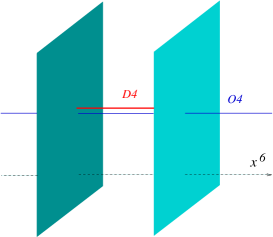
Figure 2: Hanany-Witten setup for $\mathcal{N}=2$ super Yang- Mills with orthogonal and symplectic gauge groups.

This correspondence indicates that one can match the extensive ${\rm O}2$ and localized ${\rm O}0$ contributions to the crosscap states with respectively the left, right semi-infinite pieces of the ${\rm O}4$-plane and the finite ${\rm O}4$ piece in between. From this point of view it is natural to have both the ${\rm O}2$ and ${\rm O}0$ contributions to ${\rm O}_{B}$, because each of them separately would correspond to an ${\rm O}4$-plane ending on a fivebrane, which is certainly not a consistent configuration.

Moreover it is known [39] that the parts of the O4-plane on each side of the NS5-brane carry opposite r-r charge. If one starts with two NS5-branes on top of each other and an O4⁺ plane as in fig. 2 and begins to separate the fivebranes in the $x^{6}$ direction, the part of the orientifold that stays between the NS5-branes is negatively charged, which requires the addition of a pair of D4-branes to ensure charge conservation across the fivebranes. It should be possible to reproduce this feature from the details of our ${\rm O}_{B}$ crosscap state. We will see below that the couplings to closed string modes of the localized and extended parts of the orientifold have in fact opposite signs.

In Hanany-Witten setups one can engineer a wide class of four-dimensional gauge theories with $SU(N)$, $SO(N)$ or $Sp(N)$ gauge groups and non-chiral or chiral matter. For instance, one can obtain ${\cal N}=1$ SQCD in this way with a combination of D4- and D6-branes in type IIA. This configuration has been analyzed in the dual cigar cft language in [28, 31]. In these more general constructions ${\rm O}4$- and ${\rm O}6$-planes play an important role. It would be very interesting to investigate in general how known properties of these constructions translate in the language of the exact cft description of this paper and vice versa and what lessons we can learn in this way about gauge theory dynamics.

Some quantitative results

In order to obtain a better understanding of the properties of orientifolds in the context of Hanany-Witten setups and their relation with our work, we elaborate a bit further here on a configuration including ${\rm O}4$-planes in six-dimensional non-critical type II superstrings using an ${\rm O}_{B}$-plane similar to those constructed above.

We start with type IIA superstrings on $\mathbb{R}^{5,1}\times$ SL(2,$\mathbb{R}$)/U(1) $\!|_{2}$. The angular coordinate of the cigar for $k=2$ is asymptotically a free $U(1)$ boson at level 2. It is well-known that upon a $\mathbb{Z}_{2}$ orbifold this $U(1)$ is the same as the theory of a Dirac fermion. We therefore define special combinations of the SL(2,$\mathbb{R}$)/U(1) characters at level $k=2$ that appear naturally in the fermionic description; let us consider the example of the identity character

$$Ch^{\textsc{nc}}_{\mathbb{I}}(\tau){a\atopwithdelims[ ]b}=e^{\frac{i\pi ab}{2}}\sum_{r\in\mathbb{Z}}e^{i\pi rb}ch_{\mathbb{I}}(r;\tau){a\atopwithdelims[ ]b}$$ (4.25)

and the continuous representations

$$Ch^{\textsc{nc}}_{c}(P;\tau){a\atopwithdelims[ ]b}=e^{\frac{i\pi ab}{2}}\sum_{r\in\mathbb{Z}}e^{i\pi rb}ch_{c}(P,r+\nicefrac{{a}}{{2}};\tau){a\atopwithdelims[ ]b}~{}.$$ (4.26)

As far as the $[a,b]$ labels are concerned, these characters are such that their modular transformation is similar to that of two left-moving complex fermions. The usual momentum and winding of the cigar are

$$n=r+\bar{r}+\frac{a+\bar{a}}{2}\quad,\qquad w=\frac{r-\bar{r}}{2}+\frac{a-\bar{a}}{4}~{},$$ (4.27)

where $\bar{r}$ enters into the definition of the right-moving analogue of (4.26). Since we are dealing with an asymmetric orbifold of the cigar, $n$ and $w$ are not necessarily integer. In the context of two parallel fivebranes, the momentum $n$ of the cigar (which is conserved) corresponds to the (unbroken) rotational symmetry in the plane $(x^{8},x^{9})$ while the fractional winding symmetry corresponds to the (broken to $\mathbb{Z}_{2}$) rotational symmetry in the plane $(x^{6},x^{7})$ where the fivebranes have been separated [72, 59]. Since we are dealing here with an asymmetric $\mathbb{Z}_{2}$ orbifold of the cigar, acting precisely as shifts along $\phi$, the distinction between O_B and $\tilde{\rm O}_{B}$ is intertwined with the details of the gso projection. We find that the O_B orientifold seems to be the relevant parity here as the $\tilde{\rm O}_{B}$ amounts, in the fermionized picture, to reversing the gso projection for one of the complex fermions in the transverse direction to the fivebranes.

Using the set of characters defined above one can write the torus amplitude of the type IIA non-critical superstring theory of interest as

$$\mathcal{T}=V\int_{\mathcal{F}}\frac{\text{d}\tau\text{d}\bar{\tau}}{4\tau_{2}^{2}}\frac{1}{(8\pi^{2}\tau_{2})^{6}\eta^{4}\bar{\eta}^{4}}\,\frac{1}{2}\sum_{a,b\in\mathbb{Z}_{2}}\frac{1}{2}\sum_{\bar{a},\bar{b}\in\mathbb{Z}_{2}}(-)^{a+b+\bar{a}+\bar{b}+\bar{a}\bar{b}}\frac{\vartheta^{2}{a\atopwithdelims[ ]b}\bar{\vartheta}^{2}{\bar{a}\atopwithdelims[ ]\bar{b}}^{2}}{\eta^{2}\bar{\eta}^{2}}\ \times\\ \times\ \int_{0}^{\infty}\!\!\!\text{d}P\ Ch^{\textsc{nc}}_{c}(P;\tau){a\atopwithdelims[ ]b}\bar{Ch}^{\textsc{nc}}_{c}(P;\bar{\tau}){\bar{a}\atopwithdelims[ ]\bar{b}}~{},$$ (4.28)

where $\mathcal{F}$ is the PSL(2,$\mathbb{Z}$) fundamental domain. Now let us add $N$ D4-branes suspended between the NS5-branes. In our exact cft setup each D4 has four Neumann boundary conditions in the six flat directions of $\mathbb{R}^{5,1}$ and is a D0-brane on the cigar part of the worldsheet cft. Using the above modified set of coset characters, one requires for these branes the annulus amplitude

$$\mathcal{A}=N^{2}\,V_{4}\int\frac{\text{d}t}{2t}\frac{1}{(16\pi^{2}t)^{4}\eta^{4}}\ \frac{1}{2}\sum_{a,b\in\mathbb{Z}_{2}}(-)^{a+b}\frac{\vartheta^{2}{a\atopwithdelims[ ]b}}{\eta^{2}}Ch^{\textsc{nc}}_{\mathbb{I}}(it){a\atopwithdelims[ ]b}\,.$$ (4.29)

In addition, we consider an O_B orientifold of the cigar with four Neumann dimensions in $\mathbb{R}^{5,1}$. Requiring again similar modular properties as those of two Dirac fermions we define the hatted version of the characters (4.25) as follows:

$$\widehat{Ch}^{\textsc{nc}}_{\mathbb{I}}(it){a\atopwithdelims[ ]b} =e^{\frac{i\pi}{4}(1-a^{2})}e^{\frac{i\pi ab}{2}}\sum_{n\in\mathbb{Z}}e^{i\pi nb}ch_{\mathbb{I}}(n;it+\nicefrac{{1}}{{2}}){a\atopwithdelims[ ]b}$$

$$=e^{\frac{i\pi(ab-1)}{2}+\frac{i\pi a}{4}}\sum_{n\in\mathbb{Z}}e^{i\pi\left(n(b+1)+\frac{n^{2}+an}{2}\right)}\widehat{ch}_{\mathbb{I}}(n;it){a\atopwithdelims[ ]b}\,.$$ (4.30)

These hatted characters are such that the orientifold action on the fermionized $U(1)_{2}$ is similar to that on the other worldsheet fermions. They are related non-trivially to a sum of unextended hatted characters, as defined in app. C and used in sect. 4. Indeed, in the definition (4.25, 4.26) one sums over the spectral flow orbit of the $\mathcal{N}=2$ algebra, so that the states are reorganized in terms of the extended symmetry that appears for $k\in\mathbb{Z}_{>0}$. As a consequence, states with $r\neq 0$ are considered as primaries of the unextended symmety, but are not primaries of the extended one. This is why the character (4.30) contains the phase factor $\exp{i\pi(r^{2}/2+ar)}$ if one compares with app. C. The general guideline is to obtain modular properties consistent with the generalized gso projection and spacetime supersymmetry.

Accordingly, we make the following Möbius strip amplitude ansatz for an orientifold extended along $\mathbb{R}^{3,1}$ and of the O_B type in SL(2,$\mathbb{R}$)/U(1) – expected to correspond to an O4-plane in the five-branes background – and $N$ D4-branes in the non-critical superstring (for the overall phase in the ns sector, see footnote 20):

$$\mathcal{M}=N\epsilon\,V_{4}\int\frac{\text{d}t}{2t}\frac{1}{(16\pi^{2}t)^{4}\eta^{4}(it+\nicefrac{{1}}{{2}})}\frac{1}{2}\sum_{a,b\in\mathbb{Z}_{2}}e^{\frac{i\pi(1-a^{2})}{4}}(-)^{a+b}\frac{\vartheta^{2}{a\atopwithdelims[ ]b}(it+\nicefrac{{1}}{{2}})}{\eta^{2}(it+\nicefrac{{1}}{{2}})}\widehat{Ch}^{\textsc{nc}}_{\mathbb{I}}(it){a\atopwithdelims[ ]b}~{}.$$ (4.31)

In this expression $\epsilon=\pm 1$ denotes the usual sign ambiguity of the Möbius strip amplitude. We can modular transform this result to the closed string channel using the results of app. C. Then we obtain

$$\mathcal{M}=N\epsilon\,V_{4}\int\frac{\text{d}t}{t^{3}}\frac{1}{(16\pi^{2})^{4}\eta^{4}(-\frac{i}{4t}+\frac{1}{2})}\ \frac{1}{2}\sum_{a,b\in\mathbb{Z}_{2}}(-)^{b+ab+1}\frac{\vartheta^{2}{a\atopwithdelims[ ]a-b+1}(-\nicefrac{{i}}{{4t}}+\nicefrac{{1}}{{2}})}{\eta^{2}(-\nicefrac{{i}}{{4t}}+\nicefrac{{1}}{{2}})}\ \times\\ \times\ \sqrt{2}\int_{0}^{\infty}\!\!\!\frac{\text{d}P}{\cosh\pi P}\left[\cosh\frac{\pi P}{2}-\sinh\frac{\pi P}{2}\,\sinh\pi P\right]e^{\frac{i\pi(a^{2}-1)}{4}}\widehat{Ch}^{\textsc{nc}}_{c}\left(P,-\frac{1}{4it}\right){a\atopwithdelims[ ]a-b+1}~{}.$$ (4.32)

There is also a contribution of $j=1$ discrete characters in this expression which we will not write out explicitly. We observe that the contributions of the O2- and O0-planes, respectively the first and second terms inside the square brackets, couple to the same characters (in contrast with the un-orbifoldized SL(2,$\mathbb{R}$)/U(1) theory discussed in subsection 4.1). More importantly, these two parts of the orientifold wave-function come with opposite signs, suggesting as discussed above that, while the O2-part (mapped to the semi-infinite parts of the O4-plane outside the five-branes) corresponds to an O4⁺ plane, the O0-part (mapped to the segment of the O4-plane between the five-branes) is similar to an O4^- plane.

Using the explicit expression for the continuous representation characters, see app. A, one finds, using Jacobi’s abstruse identity, that the amplitude vanishes as expected from supersymmetry:

$$\mathcal{M}=N\epsilon\,V_{4}\int\frac{\text{d}t}{t^{3}}\frac{1}{(16\pi^{2})^{4}\eta^{9}(-\frac{i}{4t}+\frac{1}{2})}\ \ \times\\ \times\ \frac{1}{\sqrt{2}}\int_{0}^{\infty}\!\!\!\frac{\text{d}P}{\cosh\pi P}\left(\cosh\frac{\pi P}{2}-\sinh\frac{\pi P}{2}\,\sinh\pi P\right)e^{-\frac{\pi}{4t}P^{2}}\ \Big{[}\vartheta_{3}^{4}-\vartheta_{4}^{4}-\vartheta_{2}^{4}\Big{]}(-\tfrac{i}{4t}+\tfrac{1}{2})=0\,.$$ (4.33)

We leave a more detailed analysis of these results and the corresponding spacetime physics for future work.

5 A-type orientifolds on the cigar: an O1-plane

In this last section we construct A-type orientifolds of the SL(2,$\mathbb{R}$)/U(1) coset cft. In the axial coset (the cigar) they correspond to O1-planes extending in the asympotic region, with a geometry similar to the lower-left picture of fig. 1. Algebraically they are related to the parity $\mathcal{P}_{1}=\tau_{1}\Omega_{B}$, using the notation of sect. 3. In terms of the natural $\mathcal{N}=2$ parity $\Omega_{A}$ we can write $\mathcal{P}_{1}$ as $(-)^{\bar{F}}\Omega_{A}$. Let us recall that the ”twisted” version of this orientifold, the $\tau_{4}\Omega$ parity of sect. 3, is non-perturbatively inconsistent because it projects out the winding condensate (2.5).

Although A-type boundary conditions are usually more straightforward to deal with, a problem arises when one tries to apply modular boostrap methods to this case. Indeed, the D0-brane of the cigar has B-type boundary conditions, therefore its Möbius strip amplitude with the ${\rm O}1$-plane would involve mixed boundary conditions and would either vanish or turn the computation of the corresponding $\mathcal{P}$-matrix into a complicated problem. We could try to circumvent this difficulty by starting with the Möbius strip amplitude for an A-type brane, i.e. a D1-brane. However the latter has a continuous open string spectrum, with a regularized density of states that contains most of the information about the boundary state. Previous experience teaches us that dealing with this volume divergence is quite intricate.

Our strategy to solve this problem will be to study this orientifold in the parent wzw model SL(2,$\mathbb{R}$) – or more conveniently in its Euclidean counterpart H${}_{3}^{+}$ – rather than in its cosets. Indeed, it is rather straightforward to ”lift” the results of section 4 concerning the ${\rm O}2$-planes of the axial coset SL(2,$\mathbb{R}$)/U(1) to H${}_{3}^{+}$. There the problem is simpler since the ${\rm O}2$-plane and the O1-plane are related to each other by an SL(2,$\mathbb{C}$) relation, as the corresponding D-branes [55]. This will furthermore allow us to compare with the conformal bootstrap results in H${}_{3}^{+}$ that were obtained in [33].

The asymptotic Klein bottle amplitude

We can gain intuition about the ${\rm O}1$-plane by looking at the way the orientifold projection acts on the closed string spectrum of the cigar and computing the Klein bottle amplitude in the direct channel. As in sect. 4 we consider first the extensive part of the torus amplitude. The contribution of the finite regularized density of states will be computed later using the exact crosscap state. There we will also see that the ${\rm O}1$-plane couples only to the continuous representations.

The leading part of the torus amplitude with a type 0B modular invariant appears in eqn. (4.1). Following the geometric and algebraic descriptions of sect. 3, we find that the parity $\mathcal{P}_{1}=(-)^{\bar{F}}\tau_{1}\Omega$ acts on an ns-ns primary state $|P;n,w\rangle\otimes|0\rangle_{\textsc{ns-ns}}$ as follows:

$$\mathcal{P}_{1}\ :\quad|P;n,w\rangle\otimes|0\rangle_{\textsc{ns}}\ \longrightarrow\ |P;-n,w\rangle\otimes|0\rangle_{\textsc{ns-ns}}\,.$$ (5.1)

The trace over the bosonic oscillators in unaffected, since $\Omega$ requires the pairing of left- and right-movers and the geometric involution $\tau_{1}$ leaves the paired combinations invariant. The parity, including the $(-)^{\bar{F}}$ factor, acts on worldsheet fermions as

$$\mathcal{P}_{1}\ :\quad\psi^{\epsilon}\to\bar{\psi}^{-\bar{\epsilon}}\ ,\quad\quad\bar{\psi}^{\bar{\epsilon}}\to-\psi^{-\epsilon}\,,$$ (5.2)

so that each term of the winding $\mathcal{N}=2$ Liouville interaction, see eqn. (2.5), is separately invariant. Because of the diagonal gso projection only states with $F+\bar{F}=0\mod 2$ contribute to the torus amplitude. One can similarly trace the action in the r-r sector. The Klein bottle amplitude reads:

$$\mathcal{K}_{\text{O1}}(t)=V\sum_{a\in\mathbb{Z}_{2}}\int_{0}^{\infty}\text{d}P\,\sum_{w\in\mathbb{Z}}e^{-4\pi t\left(\frac{P^{2}}{k}+\frac{kw^{2}}{4}\right)}\frac{\vartheta{a\atopwithdelims[ ]0}(2it)}{\eta(2it)^{3}}$$ (5.3)

Using the standard $S$-modular transformation (A.3), one finds in the transverse channel

$$\tilde{\mathcal{K}}_{\text{O1}}(t)=\frac{V}{2}\sum_{a\in\mathbb{Z}_{2}}\sum_{n\in\mathbb{Z}}\delta_{n,0}^{(2)}e^{-\frac{\pi}{t}\frac{n^{2}}{4k}}\ \frac{\vartheta{0\atopwithdelims[ ]a}(-\frac{1}{2it})}{\eta(-\frac{1}{2it})^{3}}$$ (5.4)

Therefore the orientifold plane sources only even momentum states in the ns-ns sector in this context.

The crosscap wave-function by rotation

In order to obtain the full crosscap state of the ${\rm O}1$-plane in SL(2,$\mathbb{R}$)/U(1) , we start from the ${\rm O}2$ crosscap wave-function in H${}_{3}^{+}$. The latter is obtained using the coset construction backwards, as explained in the beginning of this section, from our results for the ${\rm O}_{B}$-plane in the coset model. Let us write the one-point functions on $\mathbb{RP}_{2}$ for the O2/O0-plane, for generic $j$ in the ns-ns sector as follows:

$$\langle V^{\textsc{ns-ns}}_{j,m\,\bar{m}}(z,\bar{z})\rangle_{\text{O2}}=\frac{C^{\text{O2}}_{j\,m\,\bar{m}}}{|1+z\bar{z}|^{2\Delta_{jm\bar{m}}}\!\!\!\!\!\!\!\!\!\!\!\!\!\!}$$ (5.5)

with

$$C^{\text{O2}}_{j\,m\,\bar{m}}=\mathcal{N}_{k}e^{\frac{i\pi}{4}}\delta_{m,\bar{m}}\nu^{\nicefrac{{1}}{{2}}-j}\Gamma\left(1+\frac{1-2j}{k}\right)\ \times\\ \times\ \left\{\cos\frac{\pi(j-\nicefrac{{1}}{{2}})}{k}\Gamma(1-2j)\left(\frac{\Gamma(j-m)}{\Gamma(1-j-m)}+\frac{\Gamma(j+m)}{\Gamma(1-j+m)}\right)-\right.\\ \left.-i\sin\frac{\pi(j-\nicefrac{{1}}{{2}})}{k}\,\frac{\Gamma(j+m)\Gamma(j-m)}{\Gamma(2j)}\right\}\,.$$ (5.6)

This expression is obtained from the $\mathcal{P}$-matrix element of one unextended character, see app. C, analytically continued in the complex $j$-plane. In the axial/vector coset, there will be some condition over $m$ and $\bar{m}$ ($i.e.$ $m\pm\bar{m}=0$), otherwise this result applies readily (up to a $k$-dependent normalization factor $\mathcal{N}_{k}$) to the parent H${}_{3}^{+}$ theory.

Since we consider below the H${}_{3}^{+}$ model, for which the Euclidean time is non-compact, there is no room for an analogue of the $\tilde{\rm O}_{B}$ orientifold. It will be more convenient here to use the $(x,\bar{x})$ basis, related to the $(m,\bar{m})$ basis through the Mellin transform (see e.g. [55]):

$$\hat{f}_{m\,\bar{m}}=\frac{1}{4\pi^{2}}\int_{\mathbb{C}}\text{d}^{2}x\ x^{j-1+m}\,\bar{x}^{j-1+\bar{m}}f(x,\bar{x})$$ (5.7)

Therefore we can re-express the crosscap couplings as

$$C^{\text{O2}}_{j\,x\,\bar{x}}=4\pi\mathcal{N}_{k}\,\nu^{\nicefrac{{1}}{{2}}-j}\Gamma\left(1+\frac{1-2j}{k}\right)\ \times\\ \times\ \left\{\cos\frac{\pi(j-\nicefrac{{1}}{{2}})}{k}|1-x\bar{x}|^{-2j}-i\sin\frac{\pi(j-\nicefrac{{1}}{{2}})}{k}\,|1+x\bar{x}|^{2j}\right\}~{}.$$ (5.8)

Comparing this expression to the one-point functions for the branes found in [55] in H${}_{3}^{+}$, one confirms the geometrical interpretation outlined in sect. 4. The first term corresponds to an H₂ orientifold in H${}_{3}^{+}$, since it has the geometry of an H₂ brane with no magnetic field, while the second term corresponds to a point-like orientifold with the same geometry as a ”spherical brane” in H${}_{3}^{+}$ with zero radius. As argued previously from several point of views, these orientifolds are tied together in the coset and cannot make sense separately.

Now, in order to obtain the Euclidean AdS₂ orientifold in Euclidean AdS₃, we consider an SL(2,$\mathbb{C}$) rotation acting on the SL(2,$\mathbb{C}$)/SU(2) eigen-functions as follows:

$$U\ :\quad\Phi^{j}_{x\bar{x}}\ \longrightarrow\ \left|\frac{x+1}{\sqrt{2}}\right|^{-4j}\Phi^{j}_{\frac{x-1}{x+1},\frac{\bar{x}-1}{\bar{x}+1}}$$ (5.9)

Under this rotation, the crosscap wave-function (5.8) transforms as:

$$C^{\text{O2}}_{j\,x\,\bar{x}}\ \longrightarrow 4\pi\mathcal{N}_{k}\,\nu^{\nicefrac{{1}}{{2}}-j}\ \Gamma\left(1+\frac{1-2j}{k}\right)\ \times\\ \times\ \left\{\cos\frac{\pi(j-\nicefrac{{1}}{{2}})}{k}|x+\bar{x}|^{-2j}-i\sin\frac{\pi(j-\nicefrac{{1}}{{2}})}{k}\,|1+x\bar{x}|^{-2j}\right\}\,.$$ (5.10)

This result can be interpreted as follows. The first term of the crosscap wave-function that exhibits the H₂ geometry, is rotated to an orientifold with an AdS₂ geometry. The second term is invariant as it should, since the O(-1) has a point-like geometry and sits at the center of rotation.

We now come back to the axial coset SL(2,$\mathbb{R}$)/U(1) . There we would like to argue that by descent from the first term alone, i.e. the AdS₂-plane, we obtain a consistent O1-plane. First notice that the two terms of eqn. (5.10) will give rise to different boundary conditions for the $\mathcal{N}=2$ superconformal algebra (A-type for the first one and B-type for the second one). In other words, the corresponding crosscap states will be constructed out of a different set of Ishibashi states. We learned, however, in sect. 4 that an ${\rm O}0$-plane alone (this would come from the second term of eqn. (5.10)), cannot be a consistent orientifold on its own. In particular, the couplings to discrete representations will not be consistent, see app. C. Furthermore, we will see below that the first term of (5.10), after descent to the coset theory, does not contain couplings to discrete representations and therefore is free of this problem. To summarize, from the first piece we get the O1-plane wave-function in the $x$-basis

$$C^{\text{O1}}_{j\,x\,\bar{x}}=4\pi\mathcal{N}_{k}\,\nu^{\nicefrac{{1}}{{2}}-j}\Gamma\left(1+\frac{1-2j}{k}\right)\cos\frac{\pi(j-\nicefrac{{1}}{{2}})}{k}|x+\bar{x}|^{-2j}~{}.$$ (5.11)

We can now go back to the $(m,\bar{m})$ basis using the Mellin transform (5.7) and finally obtain the crosscap wave-function in the cigar for the ns-ns sector:

$$C^{\text{O1}\,\textsc{ns}}_{j\,\frac{n+kw}{2}\,\frac{n-kw}{2}}=\mathcal{N}^{\prime}_{k}\,\delta_{w,0}\ \delta_{n,0}^{(2)}\nu^{\nicefrac{{1}}{{2}}-j}\cos\frac{\pi(j-\nicefrac{{1}}{{2}})}{k}\frac{\Gamma\left(1+\frac{1-2j}{k}\right)\Gamma(1-2j)}{\Gamma(1-j+\frac{n}{2})\Gamma(1-j-\frac{n}{2})}~{}.$$ (5.12)

Up to a cosine term (which accounts for ”quantum” corrections to the semi-classical result) we have indeed the same wave-function as for a straight (i.e. with $\hat{\rho}=0$) D1-brane in the cigar, see eqn. (B.4) in app. B or ref. [22]. One can check that the crosscap wave-function is compatible with the reflection symmetry (A.7). Similarly to the D1-brane case, this crosscap wave-function does not possess couplings to discrete representations of SL(2,$\mathbb{R}$)/U(1) as we advertised above.

It is rather straightforward to obtain the wave-function in the r-r sector. Indeed, using the coset construction, the H${}_{3}^{+}/\mathbb{R}$ coset superconformal field theory can be represented as the constrained product of cfts H${}_{3}^{+}$ $\times$ U(1) $\times$ [Dirac fermion] $\times$ [ghosts] $\times$ [superghosts]. The wave-function (5.12) is written in terms of the eigenvalues of the bosonic SL(2,$\mathbb{R}$) algebra $(m_{b},\bar{m}_{b})=(m-m_{f},\bar{m}-\bar{m}_{f})$ where $(m_{f},\bar{m}_{f})$ is the same as the left- and right-fermion number of the free Dirac fermion. Therefore we find the generic wave-function (with a similar notation as in sect. 4)

$$\Psi_{{\rm O}1}\left(p,n;\left[{b\atop c}\right]\right)=\mathcal{N}^{\prime}_{k}\,e^{i\varphi(b,c)}\ \delta_{n,0}^{(2)}\nu^{-ip}\cosh\frac{\pi p}{k}\,\frac{\Gamma\left(1-\frac{2ip}{k}\right)\Gamma(-2ip)}{\Gamma(\frac{1}{2}-ip+\frac{n+b}{2})\Gamma(\frac{1}{2}-ip-\frac{n+b}{2})}\,.$$ (5.13)

We will fix below the normalization of the wave-function (5.12) and the phases $\varphi(b,c)$ in the different fermionic sectors by computing different amplitudes.

Comparison with conformal bootstrap

Partial results for the conformal bootstrap of Euclidean AdS₂ orientifold planes in H${}_{3}^{+}$ were obtained in [33]. The author of this paper considered the auxillary two-point function $\langle\Phi^{j}_{x\bar{x}}\Phi^{-\nicefrac{{1}}{{2}}}_{y\bar{y}}\rangle_{\mathbb{RP}_{2}}$ with a degenerate representation $j=-\nicefrac{{1}}{{2}}$ in order to constrain the form of the crosscap wave-function. In this way he proposed couplings to the continuous representations which are identical to our result (5.11) when evaluated at $j=\nicefrac{{1}}{{2}}+ip$. However we should emphasize that the conformal bootstrap method used there was not powerfull enough in order to fully determine the crosscap wave-function. Our approach allows to remove this freedom and find the full wave-function, up to an overall normalization that is fixed by a Cardy-like condition.

Asymptotic Möbius strip amplitude for the D1-brane

We will study here the effect of the parity $\mathcal{P}_{1}$ on open string sectors attached to D1-branes of the cigar. As reviewed in sect. 2 these branes, which extend to the asymptotic region, are characterized by two parameters $(\hat{\rho},\hat{\phi})$. From eqn. (2.8) we observe that $\hat{\rho}$ parameterizes the position of the turning point of the brane near the tip of the cigar at $\rho=0$. Since the ${\rm O}1$-plane corresponding to $\mathcal{P}_{1}$ has a similar geometry as the D1-brane with $\hat{\rho}=0$, it is clear that only the D1-branes with $\hat{\rho}=0$ are invariant.

The second parameter $\hat{\phi}$ gives the position of the brane on the transverse circle in the asymptotic region $\rho\to\infty$ where the geometry is approximated by a semi-infinite cylinder. The brane possesses two branches, at ($\hat{\phi},\hat{\phi}+\pi)$. Consequently, there are two kinds of open strings, one kind with integral winding where both ends of the string are on the same branch, and another kind with half-integral winding where the open string has one end on each branch. The parity $\mathcal{P}_{1}$ as defined in sect. 2 corresponds at infinity to a pair of O1-planes of equal tension located at $\phi=0,\pi$.

In the asymptotic region, one finds that the action of the parity on open string states with integral winding $w$ is

$$\mathcal{P}_{1}\ :\quad|w\rangle_{\hat{\phi},\hat{\phi}}\longrightarrow|w\rangle_{-\hat{\phi},-\hat{\phi}}\,.$$ (5.14)

There are invariant states provided $\hat{\phi}=0\mod\pi$. Since the brane has two branches there is actually only one possibility. Let us now consider open strings with half-integral windings. The action of the parity reads

$$\mathcal{P}_{1}\ :\quad|w\rangle_{\hat{\phi},\hat{\phi}+\pi}\longrightarrow|w\rangle_{\pi-\hat{\phi},-\hat{\phi}}\,.$$ (5.15)

In this case, invariant open string states exist when $\hat{\phi}=\pi/2\mod\pi$. Accordingly we will distinguish between two different cases: the case of a D1-brane with $\hat{\phi}=0$ and the case with $\hat{\phi}=\pi/2$. In the first case, integral windings will contribute to the Möbius strip amplitude, in the second half-integral windings will contribute.

Let us start with the first case. The annulus amplitude for a D1-brane, see [22, 23], comes with two different regularized densities of states for the integral and half-integral winding modes depending on the parameter $\hat{\rho}$. The extensive part of the open string partition function, however, is the same in both cases and can be written as

$$\mathcal{A}_{\hat{\phi}=0\,{a_{1}\atopwithdelims[ ]b_{1}}\ ;\ \hat{\phi}=0\,{a_{2}\atopwithdelims[ ]b_{2}}}(t)=\\ V\delta_{b_{1},b_{2}}^{(2)}\int_{0}^{\infty}\!\!\!\text{d}P\sum_{w\in\mathbb{Z}}\left\{ch_{c}(P,kw;it){a_{1}-a_{2}\atopwithdelims[ ]b_{1}}+ch_{c}(P,k(w+\nicefrac{{1}}{{2}});it){a_{1}-a_{2}\atopwithdelims[ ]b_{1}}\right\}$$ (5.16)

Acting with the parity $\mathcal{P}_{1}$ one finds the Möbius strip amplitude:

$$\mathcal{M}_{\hat{\phi}=0\,{a\atopwithdelims[ ]b}}=V\delta_{b,0}^{(2)}\,\int_{0}^{\infty}\!\!\!\text{d}P\sum_{c\in\mathbb{Z}_{2}}\sum_{w\in\mathbb{Z}}\widehat{ch}_{c}(P,kw;it){0\atopwithdelims[ ]c}$$ (5.17)

With the help of eqn. (C.28) we perform now a ${\cal P}$-modular transformation to the closed string channel to obtain the amplitude

$$\tilde{\mathcal{M}}_{\hat{\phi}=0\,{a\atopwithdelims[ ]b}}(t)=V\delta_{b,0}^{(2)}e^{\frac{i\pi}{4}}\,\sum_{c\in\mathbb{Z}_{2}}\sum_{n\in\mathbb{Z}}e^{-\frac{i\pi c}{2}}\delta_{n,0}^{(2)}\,\widehat{ch}_{c}\left(0,\frac{n}{2};-\frac{1}{4it}\right){0\atopwithdelims[ ]1-c}=$$ (5.18a)

$$=V\sum_{c\in\mathbb{Z}_{2}}\sum_{n\in\mathbb{Z}}\Phi_{D1;(\hat{\rho}=0;\hat{\phi}=0){a\atopwithdelims[ ]-b}}^{\text{sing}}(0;-n)\Psi_{{\rm O}_{A}}^{\text{sing}}\left(0,n;\left[{b\atop c}\right]\right)\widehat{ch}_{c}\left(0,\frac{n}{2};-\frac{1}{4it}\right){b\atopwithdelims[ ]c-a}\,.$$ (5.18b)

In (5.18b) only the residues of the poles that the wave-functions have for $p\to 0$ appear, since we started with the extensive part of the annulus amplitude. Using the brane wave-function (B.4) one finds in the limit $p\to 0$

$$\Phi_{D1;(\hat{\rho}=0;\hat{\phi}=0){a\atopwithdelims[ ]b}}(p;n)\stackrel{{\scriptstyle p\to 0}}{{\sim}}\delta_{n,0}^{(2)}\frac{\nu^{-ip}\,\Gamma(0)}{\sqrt{2}\Gamma(\frac{1}{2}-\frac{n+b}{2})\Gamma(\frac{1}{2}+\frac{n+b}{2})}=\frac{(-)^{\frac{n}{2}}}{\sqrt{2}}\delta_{n,0}^{(2)}\delta_{b,0}^{(2)}\,\nu^{-ip}\,\frac{\Gamma(0)}{\pi}\,.$$ (5.19)

In this way, we obtain the volume diverging part of the crosscap wave-function as

$$\Psi_{{\rm O}_{A}}^{\text{sing}}\left(0,n;\left[{b\atop c}\right]\right) =\sqrt{2}\delta_{b,0}^{(2)}\delta_{n,0}^{(2)}(-)^{\frac{n}{2}}e^{\frac{i\pi(1-2c)}{4}}\ \nu^{-ip}~{}.$$ (5.20)

We observe that it agrees exactly with the singular part of eqn. (5.13) provided we make the choice

$$\mathcal{N}_{k}^{\prime}\,e^{i\varphi(b,c)}=\sqrt{2}e^{\frac{i\pi(1-2c)}{4}}~{}.$$ (5.21)

Actually, in order to obtain an orientifold with real tension in the string theory context, one can use the phase ambiguity in the definition of the crosscaps in the ns-ns sector that was mentioned in footnote 20. This done, the exact crosscap wave-function of the ${\rm O}1$-plane in the SL(2,$\mathbb{R}$)/U(1) super-coset is

$$\Psi_{{\rm O}_{A}}\left(p,n;\left[{b\atop c}\right]\right)=\sqrt{2}e^{\frac{i\pi(1-b-c)}{2}}\delta_{n,0}^{(2)}\nu^{-ip}\cosh\frac{\pi p}{k}\,\frac{\Gamma\left(1-\frac{2ip}{k}\right)\Gamma(-2ip)}{\Gamma(\frac{1}{2}-ip+\frac{n+b}{2})\Gamma(\frac{1}{2}-ip-\frac{n+b}{2})}\,.$$ (5.22)

As with the D1-brane wave-function there is no coupling to the states of discrete representations of SL(2,$\mathbb{R}$)/U(1) .

The case of the D1-brane with $\hat{\phi}=\frac{\pi}{2}$ can be treated along the same lines. First, one obtains in the open string channel a Möbius strip amplitude similar to eqn. (5.17) but with half-integral windings only (i.e. in (5.17) $w$ should be replaced with $w+\nicefrac{{1}}{{2}}$). In the dual channel, one gets eqn. (5.18a) with an extra phase $e^{i\pi n/2}$. This phase is precisely canceled by the phase $e^{-in\hat{\phi}}$ of the D1-brane wave-function (see eqn. (B.4)) since $\hat{\phi}=\pi/2$. This is a nice check of consistency, because the crosscap wave-function (5.22) cannot depend on the specific brane that we use in the derivation.

Regularized Klein bottle amplitude

Having at our disposal the exact crosscap state for the ${\rm O}1$-plane we can compute the Klein bottle amplitude beyond the asymptotic region (5.3) and thus determine also the non-trivial regularized density of states. We start with the transverse channel amplitude

$$\tilde{\mathcal{K}}_{{\rm O}1}(t) =\sum_{c\in\mathbb{Z}_{2}}\int_{0}^{\infty}\!\!\!\text{d}p^{\prime}\sum_{n\in\mathbb{Z}}\Psi_{{\rm O}_{A}}\left(-p^{\prime},-n;\left[{0\atop-c}\right]\right)\Psi_{{\rm O}_{A}}\left(p^{\prime},n;\left[{0\atop c}\right]\right)ch_{c}\left(p^{\prime},\frac{n}{2};-\frac{1}{2it}\right){0\atopwithdelims[ ]c}$$

$$=-\frac{1}{2k}\sum_{c\in\mathbb{Z}_{2}}\int_{0}^{\infty}\!\!\!\frac{\text{d}p^{\prime}}{\tanh\pi p^{\prime}\,\tanh\frac{\pi p^{\prime}}{k}}\sum_{N\in\mathbb{Z}}ch_{c}\left(p^{\prime},N;-\frac{1}{2it}\right){0\atopwithdelims[ ]c}~{}.$$ (5.23)

We observe that the integral over $p^{\prime}$ has an ir divergence, which corresponds to the infinite volume of the cigar manifold. Taking the leading, divergent piece – proportional to $\delta(p^{\prime})$ – one recovers the direct channel Klein bottle amplitude (5.3). The finite part of the Klein bottle amplitude in the direct channel reads

$$\mathcal{K}_{{\rm O}_{A}}=-\sum_{c\in\mathbb{Z}_{2}}\sum_{w\in\mathbb{Z}}\int_{0}^{\infty}\!\!\!\text{d}P\ \rho_{K}(P)\ ch_{c}\left(P,\frac{kw}{2};2it\right){c\atopwithdelims[ ]0}\,,$$ (5.24)

with regularized density of states

$$\rho_{K}(P)=\frac{1}{2i\pi}\frac{\text{d}}{\text{d}P}\ i\int_{0}^{\infty}\frac{\text{d}y}{y}\left[\frac{\sin\frac{4Py}{k}}{2\tanh y\tanh\frac{y}{k}}-\frac{2P}{y}\right]\,.$$ (5.25)

Such a density of states is not related to the closed string reflection amplitude as in the torus case [66, 67, 68]. Indeed, the density of states that appears in the latter is

$$\rho_{\mathcal{T}}(P,n)=\frac{1}{2i\pi}\frac{\text{d}}{\text{d}P}\log\frac{\Gamma(\nicefrac{{1}}{{2}}-iP+n)}{\Gamma(\nicefrac{{1}}{{2}}+iP+n)}~{}.$$ (5.26)

and is naturally related to the closed string reflection amplitude given by eqn. (A.6). In particular, this expression does not depend on the level $k$ in contrast with (5.25). This non-trivial (and perhaps counter-intuitive) action of orientifolds on density of states is a general feature (for related remarks in the case of the O2-plane see sect. 4).

Appendix A Conventions and useful material

Free fermions

Let us consider first the theory of a free Dirac fermion. We define the usual theta-functions as

$$\vartheta{a\atopwithdelims[ ]b}(\tau,\nu)=\sum_{n\in\mathbb{Z}}q^{\frac{1}{2}(n+\frac{a}{2})^{2}}e^{2i\pi(n+\frac{a}{2})(\nu+\frac{b}{2})},$$

where $q=e^{2\pi i\tau}$. The fermionic characters are written as $\vartheta{a\atopwithdelims[ ]b}(\tau;\nu)/\eta(\tau)$. The ns sector (resp. r sector) is given by $a=0$ (resp. $a=1$), while characters with $b=1$ have a phase $e^{i\pi F}$ inserted in the trace. Their modular transformations read

$$\frac{\vartheta{a\atopwithdelims[ ]b}(-\nicefrac{{1}}{{\tau}};-\nicefrac{{\nu}}{{\tau}})}{\eta(-\nicefrac{{1}}{{\tau}})} =e^{i\pi(\nicefrac{{\nu^{2}}}{{\tau}}-\nicefrac{{ab}}{{2}})}\frac{\vartheta{-b\atopwithdelims[ ]a}(\tau;\nu)}{\eta(\tau)}$$ (A.1a)

$$\frac{\vartheta{a\atopwithdelims[ ]b}(\tau+1;\nu)}{\eta(\tau+1)} =e^{-i\frac{\pi}{4}a(a-2)}\frac{\vartheta{a\atopwithdelims[ ]a+b-1}(\tau;\nu)}{\eta(\tau)}$$ (A.1b)

Characters of the non-minimal $\mathcal{N}=2$ superconformal algebra

The characters of the SL(2,$\mathbb{R}$)/U(1) super-coset at level $k$ are characters of the $\mathcal{N}=2$ superconformal algebra with $c=3+6/k$. They come in different classes corresponding to irreducible representations of the SL(2,$\mathbb{R}$) algebra in the parent theory. In all cases the quadratic Casimir of the representations is $c_{2}=-j(j-1)$. Here we summarize the basic representations.

First we consider the continuous representations with $j=1/2+ip$, $p\in\mathbb{R}^{+}$. The corresponding characters are denoted by $ch_{c}(p,m){a\atopwithdelims[ ]b}$, where the $N=2$ superconformal $U(1)_{R}$ charge of the primary is $Q=2m/k$, $m\in\mathbb{R}$. The explicit form of the characters is

$$ch_{c}(p,m;\tau,\nu){a\atopwithdelims[ ]b}=q^{\frac{p^{2}+m^{2}}{k}}e^{4i\pi\nu\frac{m}{k}}\frac{\vartheta{a\atopwithdelims[ ]b}(\tau,\nu)}{\eta^{3}(\tau)}\,.$$ (A.2)

These are also the characters that appear in a free $\mathcal{N}=2$ linear dilaton theory. Their $S$-modular transformation is straightforward

$$ch_{c}\left(P,m;-\nicefrac{{1}}{{\tau}}\right)\left[{a\atop b}\right]=\\ \frac{4}{k}e^{-\frac{i\pi ab}{2}}\int_{0}^{\infty}\text{d}P^{\prime}\int_{-\infty}^{\infty}\text{d}m^{\prime}\ e^{-\frac{4\pi imm^{\prime}}{k}}\cos\left(\frac{4\pi PP^{\prime}}{k}\right)ch_{c}\left(P^{\prime},m^{\prime};\tau\right)\left[{-b\atop a}\right]\,.$$ (A.3)

Another important class of representations comprises of discrete representations in the range $\nicefrac{{1}}{{2}}<j<\nicefrac{{k+1}}{{2}}$. The corresponding characters are usually denoted as $ch_{d}(j,r){a\atopwithdelims[ ]b}$, and have $N=2$ $U(1)_{R}$ charge $Q=(2j+2r+a)/k$ with $r\in\mathbb{Z}$. In the cigar, $j$ is quantized but not in the non-compact ${\cal N}=2$ Liouville theory. The explicit form of the discrete characters is

$$ch_{d}(j,r;\tau,\nu){a\atopwithdelims[ ]b}=q^{\frac{-(j-1/2)^{2}+(j+r+a/2)^{2}}{k}}e^{2i\pi\nu\frac{2j+2r+a}{k}}\frac{1}{1+(-)^{b}\,e^{2i\pi\nu}q^{1/2+r+a/2}}\frac{\vartheta{a\atopwithdelims[ ]b}(\tau,\nu)}{\eta^{3}(\tau)}.$$ (A.4)

The discrete primary states are

$$|j,m=j+r\rangle = |0\rangle_{\textsc{ns}}\otimes|j,m=j+r\rangle_{\textsc{bos}}\quad r\geqslant 0$$

$$|j,m=j+r\rangle = \psi^{-}_{-\frac{1}{2}}|0\rangle_{\textsc{ns}}\otimes(J^{-}_{-1})^{-r-1}|j,j\rangle_{\textsc{bos}}\quad r<0$$

While the closed string spectrum in SL(2,$\mathbb{R}$)/U(1) contains only discrete and continuous representations, the spectrum of open strings attached to localized D-branes is built on the identity representation. We denote the character of the identity representation by $ch_{\mathbb{I}}(r){a\atopwithdelims[ ]b}$. It has the form

$$ch_{\mathbb{I}}(r;\tau,\nu){a\atopwithdelims[ ]b}=\frac{(1-q)\ q^{\frac{-1/4+(r+a/2)^{2}}{k}}e^{2i\pi\nu\frac{2r+a}{k}}}{\left(1+(-)^{b}\,e^{2i\pi\nu}q^{1/2+r+a/2}\right)\left(1+(-)^{b}\,e^{-2i\pi\nu}q^{1/2-r-a/2}\right)}\frac{\vartheta{a\atopwithdelims[ ]b}(\tau,\nu)}{\eta^{3}(\tau)}.$$ (A.5)

The identity primary states in the NS sector are the identity operator $|j=0,r=0\rangle\otimes|0\rangle_{\textsc{ns}}$ and the primary states

$$|r\rangle=\psi^{+}_{-\frac{1}{2}}|0\rangle_{\textsc{ns}}\otimes(J^{+}_{-1})^{r-1}|0,0\rangle_{\textsc{bos}}\quad\text{for}\ r>0\quad\text{with}\ L_{0} =\frac{r^{2}}{k}+r-\frac{1}{2}~{},$$

$$|r\rangle=\psi^{-}_{-\frac{1}{2}}|0\rangle_{\textsc{ns}}\otimes(J^{+}_{-1})^{-r-1}|0,0\rangle_{\textsc{bos}}\quad\text{for}\ r<0\quad\text{with}\ L_{0} =\frac{r^{2}}{k}-r-\frac{1}{2}\,.$$

Reflection amplitude

Among the known structure functions of the SL(2,$\mathbb{R}$)/U(1) conformal field theory, the two-point function, or reflection amplitude, plays a special role. It reads [15] (with $\nu=\Gamma(1-\nicefrac{{1}}{{k}})/\Gamma(1+\nicefrac{{1}}{{k}})$):

$$\langle V^{1-j}_{-n\,-w}(z,\bar{z})V^{j}_{n\,w}(0,0)\rangle=|z|^{-4\Delta_{jnw}}R\left(j,\frac{n+kw}{2},\frac{n-kw}{2}\right)=$$

$$=\frac{\nu^{1-2j}}{|z|^{4\Delta_{jnw}}}\frac{\Gamma(1-2j)\Gamma(1+\frac{1-2j}{k})}{\Gamma(2j-1)\Gamma(1+\frac{2j-1}{k})}\frac{\Gamma(j+\frac{n+kw}{2})\Gamma(j+\frac{n-kw}{2})}{\Gamma(1-j+\frac{n+kw}{2})\Gamma(1-j+\frac{n-kw}{2})}\,.$$ (A.6)

As the name suggests, the reflection amplitude is related to the symmetry of the theory

$$V_{1-j,-m-\bar{m}}=R\left(j,m,\bar{m}\right)V_{j,m\bar{m}}~{}.$$ (A.7)

Extended characters

When $k$ is rational it is often convenient to define extended characters [24]. Writing $k=N/K$ with $K,N\in\mathbb{Z}_{>0}$, the extended characters are defined by partially summing over $N$ units of spectral flow. The resulting characters are characters of an extended chiral algebra similar to the extended chiral algebra of a $U(1)$ boson at rational radius squared. Explicitly, extended characters (denoted by capital letters) are defined as

$$Ch_{\star}(\star,\star){a\atopwithdelims[ ]b}(\tau;\nu)=\sum_{\ell\in\mathbb{Z}}ch_{c}\left(\star,\star\right)_{\star}{a\atopwithdelims[ ]b}(\tau;\nu+N\ell\tau)~{}.$$ (A.8)

For example, the extended characters of the continuous representations are for $k$ integer

$$Ch_{c}(P,m){a\atopwithdelims[ ]b}(\tau;\nu)=\frac{q^{\frac{P^{2}}{k}}}{\eta^{3}(\tau)}\ \Theta_{2m,k}(\tau;\nicefrac{{2\nu}}{{k}})\ \vartheta{a\atopwithdelims[ ]b}(\tau;\nu)~{}$$ (A.9)

with $2m\in\mathbb{Z}_{2k}$.

Appendix B D-brane wave-functions

For the convenience of the reader we list here the one-point functions of primary fields on the disc with boundary conditions corresponding to the D0-, D1- and D2-branes of the supersymmetric cigar. As far as D2-branes are concerned, for the purposes of the main text we will focus on the D2-branes of refs. [26, 27] that are based on the continuous representations. For a more complete list of the D-branes of ${\cal N}=2$ Liouville theory we refer the reader to the excellent presentation of [27].

The one-point function on the disc of a primary field ${\cal V}_{j,n,w}^{\left[{a\atop b}\right]}$ with quantum number $j=\frac{1}{2}+ip$, momentum $n$ and winding $w$ in the $\left[{a\atop b}\right]$-$\left[{a\atop b}\right]$ sector is

$$\left\langle{\cal V}_{p,n,w}^{\left[{a\atop b}\right]}\right\rangle_{D_{\star}}=\frac{\Phi_{D_{\star}}(j,n,w;\left[{a\atop b}\right])}{|z-\bar{z}|^{\Delta_{p,n,w;a}}}\,,$$ (B.1)

where $\Delta_{j,n,w;a}$ is the scaling dimension of the primary field and $D_{\star}$ the boundary condition of interest.

D0-branes

On the supersymmetric cigar there are (including the fermionic contribution) four D0-branes with boundary states $|D0;\left[{a\atop b}\right]\rangle$ that obey B-type boundary conditions. The one-point functions of primary fields on the disc with D0-boundary conditions are

$$\Phi_{D0;\left[{a\atop b}\right]}\left(p,n,w;\left[{a^{\prime}\atop b^{\prime}}\right]\right)=\\ =\,\delta_{n,0}\delta^{(2)}_{a^{\prime},b}\delta^{(2)}_{b^{\prime},a}~{}k^{-\frac{1}{2}}(-)^{w(a-1)}e^{-\frac{i\pi ab}{2}}\nu^{-ip}\ \frac{\Gamma(\frac{1}{2}+ip+\frac{kw}{2}+\frac{b}{2})\Gamma(\frac{1}{2}+ip-\frac{kw}{2}-\frac{b}{2})}{\Gamma(2ip)\Gamma(1+\frac{2ip}{k})}\,,$$ (B.2)

where $\nu=\nicefrac{{\Gamma(1-\frac{1}{k})}}{{\Gamma(1+\frac{1}{k})}}$.

D2-branes

There are similarly four fermionic types of D2-branes with boundary states $|D2;P,M;\left[{a\atop b}\right]\rangle$ that obey B-type boundary conditions. They are labeled by a continuous parameter $P\in\mathbb{R}_{\geq 0}$ and a half-integer $M$ and exhibit the one-point functions

$$\Phi_{D2;P,M;\left[{a\atop b}\right]}\left(p,n,w;\left[{a^{\prime}\atop b^{\prime}}\right]\right) = \delta_{n,0}\delta^{(2)}_{a^{\prime},b}\delta^{(2)}_{b^{\prime},a}~{}\sqrt{\frac{2}{k}}(-)^{w}e^{-2\pi iMw}e^{-\frac{i\pi ab}{2}}\nu^{-ip}\cos\left(\frac{4\pi pP}{k}\right)\ \times$$ (B.3)

$$\times\ \frac{\Gamma(-2ip)\Gamma(1-\frac{2ip}{k})}{\Gamma(\frac{1}{2}-ip+\frac{kw}{2}+\frac{b}{2})\Gamma(\frac{1}{2}-ip-\frac{kw}{2}-\frac{b}{2})}~{}.$$

There are no couplings to discrete states in this case.

D1-branes

Finally, there are four fermionic types of D1-branes with boundary states $|D1;\hat{\rho},\hat{\phi};\left[{a\atop b}\right]\rangle$ ($\hat{\rho}\in\mathbb{R}_{\geq 0}$, $\hat{\phi}\in[0,2\pi)$) that obey A-type boundary conditions. The corresponding one-point functions on the disc are

$$\Phi_{D1;\hat{\rho},\hat{\phi};\left[{a\atop b}\right]}\left(p,n,w;\left[{a^{\prime}\atop b^{\prime}}\right]\right) = \delta_{w,0}\delta^{(2)}_{a^{\prime},b}\delta^{(2)}_{b^{\prime},a}~{}\frac{1}{\sqrt{2}}e^{in\hat{\phi}}\nu^{-ip}\left(e^{2i\hat{\rho}p}+(-)^{n}e^{-2i\hat{\rho}p}\right)\ \times$$ (B.4)

$$\times\ \frac{\Gamma(-2ip)\Gamma(1-\frac{2ip}{k})}{\Gamma(\frac{1}{2}-ip+\frac{n}{2}+\frac{b}{2})\Gamma(\frac{1}{2}-ip-\frac{n}{2}-\frac{b}{2})}~{}.$$

There are no couplings to discrete states in this case either.

Appendix C The ${\cal P}$-matrix of unextended and extended characters

In this appendix we determine the modular transformation properties of the hatted identity representation characters under the ${\cal P}$ modular transformation

$$\tau=-\frac{1}{4it}+\frac{1}{2}\ \longrightarrow\ \tilde{\tau}=it+\frac{1}{2}~{}.$$

The results presented here are instrumental in the modular bootstrap approach of sec. 4.

We start with the hatted unextended character that appears in the open string spectrum of the D0-brane. Explicitly this character reads

$$\widehat{ch_{\mathbb{I}}}(r;\tau){a\atopwithdelims[ ]b}=e^{-i\pi(\Delta-\nicefrac{{c}}{{24}})}ch_{\mathbb{I}}(r;\tau+\nicefrac{{1}}{{2}}){a\atopwithdelims[ ]b}~{}.$$ (C.1)

Using (A.5) one finds

$$\widehat{ch_{\mathbb{I}}}(r;\tau){a\atopwithdelims[ ]b}=e^{i\pi\left(r+\frac{1}{8}+\frac{1-a}{2}-\frac{a^{2}}{8}\right)}\ \frac{\vartheta{a\atopwithdelims[ ]b}(\tau+\nicefrac{{1}}{{2}})}{\eta^{3}(\tau+\nicefrac{{1}}{{2}})}\ q^{\frac{(r+\frac{a}{2})^{2}-\frac{1}{4}}{k}}\ \times\\ \times\ \left[\frac{1}{1+e^{i\pi(b+r+\frac{a+1}{2})}q^{r+\frac{a+1}{2}}}-\frac{1}{1+e^{i\pi(b+r+\frac{a-1}{2})}q^{r+\frac{a-1}{2}}}\right]~{}.$$ (C.2)

Next inspired by [73] we introduce ”Miki’s function”

$$\mathcal{I}{a\atopwithdelims[ ]b}(N,\alpha,\beta;\tau)\equiv\sum_{s\in\mathbb{Z}+\frac{a+1}{2}}e^{2\pi is\alpha}\frac{q^{\beta s+\frac{N}{2}s^{2}}}{1+(-)^{b}e^{i\pi s}q^{s}}~{}.$$ (C.3)

One can rewrite the hatted identity character in terms of Miki’s function as

$$\widehat{ch}_{\mathbb{I}}(r;\tau,0){a\atopwithdelims[ ]b}(r;\tau)=e^{i\pi\left(r+\frac{1-a^{2}}{8}+\frac{1-a}{2}\right)}\ \frac{\vartheta{a\atopwithdelims[ ]b}(\tau+\nicefrac{{1}}{{2}})}{\eta^{3}(\tau+\nicefrac{{1}}{{2}})}\ \times\\ \times\ \ \int_{0}^{1}\text{d}\alpha\ e^{-2i\pi\alpha r}\left[e^{-i\pi\alpha(1+a)}\,\mathcal{I}{a\atopwithdelims[ ]b}\left(\frac{2}{k},\alpha,-\frac{1}{k};\tau\right)-e^{i\pi\alpha(1-a)}\,\mathcal{I}{a\atopwithdelims[ ]b}\left(\frac{2}{k},\alpha,\frac{1}{k};\tau\right)\right]~{}.$$ (C.4)

The computation of the $\mathcal{P}$-matrix elements of the identity character proceeds as follows. First, let us take care of the bosonic and fermionic oscillators

$$\frac{\vartheta{a\atopwithdelims[ ]b}\left(-\frac{1}{4it}+\frac{1}{2}\right)}{\eta^{3}\left(-\frac{1}{4it}+\frac{1}{2}\right)}=\frac{1}{2t}\,e^{\frac{i\pi}{2}(a-b+1+\frac{a-1}{2})}\frac{\vartheta{a\atopwithdelims[ ]a-b+1}\left(it+\frac{1}{2}\right)}{\eta^{3}\left(it+\frac{1}{2}\right)}~{}.$$ (C.5)

Then it will be useful to compute the quantity ${\cal I}{a\atopwithdelims[ ]b}(N,\alpha,\beta;-\frac{1}{4it})$. Explicitly, we have

$${\cal I}{a\atopwithdelims[ ]b}\left(N,\alpha,\beta;-\frac{1}{4it}\right)=\sum_{s\in\mathbb{Z}+\frac{a+1}{2}}e^{2\pi is\alpha}\frac{e^{-\frac{\pi}{2t}(\beta s+\frac{N}{2}s^{2})}}{1+e^{i\pi(s+b)}e^{-\frac{\pi s}{2t}}}\,,$$ (C.6)

which we find useful to re-express as

$${\cal I}{a\atopwithdelims[ ]b}\left(N,\alpha,\beta;-\frac{1}{4it}\right)={\cal I}_{+}{a\atopwithdelims[ ]b}\left(N,\alpha,\beta;-\frac{1}{4it}\right)\ +\ {\cal I}_{-}{a\atopwithdelims[ ]b}\left(N,\alpha,\beta;-\frac{1}{4it}\right)$$ (C.7)

with

$${\cal I}_{\pm}{a\atopwithdelims[ ]b}\left(N,\alpha,\beta;-\frac{1}{4it}\right)=\,\sum_{s\in 2\mathbb{Z}+\frac{a\pm 1}{2}}e^{2\pi is\alpha}\frac{e^{-\frac{\pi}{2t}(\beta s+\frac{N}{2}s^{2})}}{1+e^{i\pi(\frac{a+1}{2}+b)}e^{-\frac{\pi s}{2t}}}\,,$$ (C.8)

Then we observe that we can recast ${\cal I}_{\pm}$ as

$${\cal I}_{\pm}{a\atopwithdelims[ ]b}\left(N,\alpha,\beta;-\frac{1}{4it}\right)=2t\left[\int_{-\infty-i\epsilon}^{\infty-i\epsilon}\!\!\!\!\!\!-\int_{-\infty+i\epsilon}^{\infty+i\epsilon}\right]\frac{e^{-2\pi\beta x+8\pi itx(\alpha+\frac{1}{4})-4N\pi tx^{2}}\,\text{d}x}{(e^{2\pi itx}\mp e^{-2\pi i(tx-\frac{a+1}{4})})\left(1\pm e^{i\pi(\frac{a+1}{2}+b)}e^{-2\pi x}\right)}~{}.$$ (C.9)

To evaluate the rhs of (C.9) in a different way we make use of the expansions

$$\frac{1}{e^{2\pi itx}\pm e^{-2\pi i(tx-\frac{a+1}{4})}} =\sum_{n=0}^{\infty}e^{\frac{i\pi n}{2}(a\mp 1)}e^{-2\pi itx(2n+1)}~{},~{}~{}\Im x<0\,,$$ (C.10a)

$$\frac{1}{e^{2\pi itx}\pm e^{-2\pi i(tx-\frac{a+1}{4})}} =\ e^{-\frac{i\pi}{2}(a\pm 1)}\sum_{n=0}^{\infty}e^{-\frac{i\pi n}{2}(a\mp 1)}e^{2\pi itx(2n+1)}~{},~{}~{}\Im x>0\,.$$ (C.10b)

After a few steps of algebra, defining $q=e^{-2\pi t}$, we can show that

$${\cal I}_{\pm}{a\atopwithdelims[ ]b}\left(N,\alpha,\beta;-\frac{1}{4it}\right)=2t\int_{-\infty}^{\infty}\text{d}x\,\sum_{n\in\mathbb{Z}}e^{\frac{i\pi}{2}(a\pm 1)n}\frac{e^{-2\pi\beta x}}{1\pm(-)^{b}e^{\frac{i\pi}{2}(a+1)}e^{-2\pi x}}q^{2Nx^{2}-4ix(\alpha-\frac{n}{2})}\,.$$ (C.11)

Finally, shifting the contour of integration from the real line $\mathbb{R}$ to $\mathbb{R}+i(\alpha-\frac{n}{2})/N$ we obtain

$$\frac{1}{2t}{\cal I}_{\pm}{a\atopwithdelims[ ]b}\left(N,\alpha,\beta;-\frac{1}{4it}\right)={\cal J}_{cont,\pm}+{\cal J}_{disc,\pm}$$ (C.12)

with continuous contribution

$${\cal J}_{cont,\pm}=\int_{-\infty}^{\infty}dx\sum_{n\in\mathbb{Z}}e^{\frac{i\pi}{2}(a\pm 1)n}\frac{e^{-2\pi\beta(x+i\frac{2\alpha-n}{2N})}}{1\pm(-)^{b}e^{\frac{i\pi}{2}(a+1)}e^{-2\pi(x+i\frac{2\alpha-n}{2N})}}q^{2Nx^{2}+\frac{2}{N}(\alpha-\frac{n}{2})^{2}}$$ (C.13)

and discrete contribution ${\cal J}_{disc,\pm}$ that arises when we pick up the appropriate poles (this will be computed later). We are now ready to assemble the data, dealing only with the continuous pieces for the moment. By straightforward algebra we find

$$\widehat{ch}_{\mathbb{I}}(r;-\frac{1}{4it}){a\atopwithdelims[ ]b}=e^{i\pi(r+\frac{7}{8}+\frac{3a}{8}-\frac{b}{2})}\int_{-\infty}^{\infty}\text{d}P\int_{0}^{1}\text{d}\alpha\,e^{-2i\pi\alpha(r+\frac{a}{2})}\ \times\\ \times\ \sum_{n\in\mathbb{Z}}e^{\frac{i\pi an}{2}}\left[\frac{e^{\frac{i\pi n}{2}}}{1+(-)^{b}e^{\frac{i\pi}{2}(a+1)}e^{-\pi(P+i\frac{k}{2}(2\alpha-n))}}+\frac{e^{-\frac{i\pi n}{2}}}{1-(-)^{b}e^{\frac{i\pi}{2}(a+1)}e^{-\pi(P+i\frac{k}{2}(2\alpha-n))}}\right]\ \times\\ \times\ \sinh\pi\left(\frac{P}{k}-\frac{in}{2}\right)\ q^{\frac{P^{2}}{k}+k\left(\alpha-\frac{n}{2}\right)^{2}}\frac{\vartheta{a\atopwithdelims[ ]a-b+1}\left(it+\frac{1}{2}\right)}{\eta^{3}\left(it+\frac{1}{2}\right)}\ +\ \text{discrete}\,.$$ (C.14)

Let us write $n=-2\ell-\delta$ with $\delta=0,1$. We consider first the term with $\delta=0$. One can trade the summation over $\alpha$ and the sum over $\ell$ for an integral over $m=k(\ell+\alpha)$ and fold the integral over the $P$-axis:

$$\frac{1}{k}e^{i\pi(r+\frac{7}{8}+\frac{3a}{8}-\frac{b}{2})}\int_{0}^{\infty}\!\!\text{d}P\int_{-\infty}^{+\infty}\text{d}m\ \frac{q^{\frac{P^{2}+m^{2}}{k}}}{\eta^{3}\left(it+\frac{1}{2}\right)}\ \vartheta{a\atopwithdelims[ ]a-b+1}\left(it+\frac{1}{2}\right)\ \times\\ \times\ \ \frac{e^{-\frac{2i\pi}{k}m(r+\frac{a}{2})}\,\sinh 2\pi P\sinh\frac{\pi P}{k}}{\cosh\pi\left[P+i(m-\frac{a}{2})\right]\cosh\pi\left[P-i(m-\frac{a}{2})\right]}$$ (C.15)

Consider now the term with $\delta=1$. We define also $m=k(\ell+\nicefrac{{1}}{{2}}+\alpha)$ and obtain the result

$$2\,e^{i\pi(b+r-\nicefrac{{1}}{{2}})}\ \frac{1}{k}e^{i\pi(r+\frac{7}{8}+\frac{3a}{8}-\frac{b}{2})}\int_{0}^{\infty}\!\!\text{d}P\int_{-\infty}^{+\infty}\text{d}m\ \frac{q^{\frac{P^{2}+m^{2}}{k}}}{\eta^{3}\left(it+\frac{1}{2}\right)}\ \vartheta{a\atopwithdelims[ ]a-b+1}\left(it+\frac{1}{2}\right)\ \times\\ \times\ \ \frac{e^{-\frac{2i\pi}{k}m(r+\frac{a}{2})}\,\cosh\pi P\cos\pi\left(m-\frac{a}{2}\right)\cosh\frac{\pi P}{k}}{\cosh\pi\left[P+i(m-\frac{a}{2})\right]\cosh\pi\left[P-i(m-\frac{a}{2})\right]}$$ (C.16)

The full result can be recast as follows

$$\widehat{ch}_{\mathbb{I}}{a\atopwithdelims[ ]b}(r;-\frac{1}{4it})=\frac{2}{k}\,e^{i\pi\left(\frac{2a+1}{4}+\frac{b}{2}\right)}\int_{0}^{\infty}\!\!\!\!\text{d}P\int_{-\infty}^{\infty}\!\!\!\!\text{d}m\ \ \times\\ \times\ \ \frac{e^{-\frac{2i\pi}{k}m(r+\frac{a}{2})}\,\cosh\pi P\left[\cos\pi\left(m-\frac{a}{2}\right)\cosh\frac{\pi P}{k}+i(-)^{b+r}\sinh\pi P\sinh\frac{\pi P}{k}\right]}{\cosh\pi\left[P+i(m-\frac{a}{2})\right]\cosh\pi\left[P-i(m-\frac{a}{2})\right]}\ \times\\ \times\ e^{\frac{i\pi}{8}(1-a^{2})}\frac{q^{\frac{P^{2}+m^{2}}{k}}\,\vartheta{a\atopwithdelims[ ]a-b+1}\left(it+\frac{1}{2}\right)}{\eta^{3}\left(it+\frac{1}{2}\right)}+\text{discrete}\,.$$ (C.17)

In the last line we recognize an $\Omega$-twisted character for continuous representations. It allows to obtain the $\mathcal{P}$-matrix elements of the identity to the continuous representations as

$$\begin{array}[]{|l|}\hline\cr\mathcal{P}_{\mathbb{I};\,r{a\atopwithdelims[ ]b}}^{c;\,(P,m){a^{\prime}\atopwithdelims[ ]b^{\prime}}}=\frac{2}{k}\,e^{i\pi\left(\frac{2a+1}{4}+\frac{b}{2}\right)}\delta_{a,a^{\prime}}^{(2)}\delta_{a-b+1,b^{\prime}}^{(2)}\ \times\\ \phantom{aaaaaaaaaaaa}\times\ \frac{e^{-\frac{2i\pi}{k}m(r+\frac{a}{2})}\,\cosh\pi P\left[\cos\pi\left(m-\frac{a}{2}\right)\cosh\frac{\pi P}{k}+i(-)^{b+r}\sinh\pi P\sinh\frac{\pi P}{k}\right]}{\cosh\pi\left[P+i(m-\frac{a}{2})\right]\cosh\pi\left[P-i(m-\frac{a}{2})\right]}\\ \hline\cr\end{array}$$ (C.18)

Discrete representations

While shifting the contour of integration over $x$ from $\mathbb{R}$ to $\mathbb{R}+i(\alpha-\frac{n}{2})/N$ in eqn. (C.11), one picks the residues of poles corresponding to the discrete representations of the coset SL(2,$\mathbb{R}$)/U(1) that appear in the closed string spectrum. To make the identification of discrete characters easier, we rewrite the integral (C.14) as (with $\tilde{P}=2x$):

$$\frac{2}{k}e^{i\pi(r+\frac{7+3a}{8}-\frac{b}{2})}\frac{\vartheta{a\atopwithdelims[ ]a-b+1}\left(it+\frac{1}{2}\right)}{\eta^{3}\left(it+\frac{1}{2}\right)}\int\text{d}\tilde{P}~{}\text{d}m\,e^{-\frac{2i\pi m(r+\nicefrac{{a}}{{2}})}{k}}\ \times\\ \times\ \left[\sinh\frac{\pi(\tilde{P}-im)}{k}+e^{i\pi(b+r-\nicefrac{{1}}{{2}})}\cosh\frac{\pi(\tilde{P}-im)}{k}e^{-\pi(\tilde{P}-\nicefrac{{ia}}{{2}})}\right]\frac{q^{\frac{\tilde{P}(\tilde{P}-2im)}{k}}}{1+e^{-2\pi(\tilde{P}-\nicefrac{{ia}}{{2}})}}~{}.$$ (C.19)

Assuming first $m>0$, the poles occur for

$$\tilde{P}=i\left(\upsilon+\frac{1+a}{2}\right)\ ,\quad 0\leqslant\upsilon+\frac{1+a}{2}\leqslant m\ ,\quad\upsilon\in\mathbb{Z}~{}.$$ (C.20)

The sum over the residues reads

$$-\frac{2}{k}e^{i\pi(r+\frac{7+3a}{8}-\frac{b}{2})}\frac{\vartheta{a\atopwithdelims[ ]a-b+1}\left(it+\frac{1}{2}\right)}{\eta^{3}\left(it+\frac{1}{2}\right)}\sum_{\upsilon>-\frac{1+a}{2}}\int_{\upsilon+\frac{1+a}{2}}^{\infty}\text{d}m\,e^{-\frac{2i\pi m(r+\nicefrac{{a}}{{2}})}{k}}\ \times\\ \times\ \left[\sin\frac{\pi(\upsilon-m+\frac{1+a}{2})}{k}+ie^{i\pi(b+r+\upsilon)}\cos\frac{\pi(\upsilon-m+\frac{1+a}{2})}{k}\right]q^{\frac{(\upsilon+\frac{1+a}{2})(2m-\upsilon-\frac{1+a}{2})}{k}}~{}.$$ (C.21)

To proceed further we make the slicing

$$m=j+\upsilon+\frac{a}{2}+\frac{k\ell}{2}\ ,\quad\frac{1}{2}\leqslant j\leqslant\frac{k+1}{2}\ \text{and}\quad\ell=0,1,\ldots$$ (C.22)

in terms of which we rewrite eqn (C.21) as

$$-\frac{2}{k}e^{i\pi(r+\frac{7+3a}{8}-\frac{b}{2})}\frac{\vartheta{a\atopwithdelims[ ]a-b+1}\left(it+\frac{1}{2}\right)}{\eta^{3}\left(it+\frac{1}{2}\right)}\sum_{\upsilon>-\frac{1+a}{2}}\int_{\frac{1}{2}}^{\frac{k+1}{2}}\text{d}j\ \sum_{\ell=0}^{\infty}\,e^{-\frac{2i\pi}{k}(j+\upsilon+\frac{a}{2})(r+\nicefrac{{a}}{{2}})}\ \times\\ \times\ e^{-i\pi\ell(r+\nicefrac{{a}}{{2}})}q^{\ell(\upsilon+\frac{a+1}{2})}\left[\sin\left(\frac{\pi(\nicefrac{{1}}{{2}}-j)}{k}-\frac{\pi\ell}{2}\right)+ie^{i\pi(b+r+\upsilon)}\cos\left(\frac{\pi(\nicefrac{{1}}{{2}}-j)}{k}-\frac{\pi\ell}{2}\right)\right]\ \times\\ \times\ q^{\frac{-(j-\nicefrac{{1}}{{2}})^{2}+(j+\upsilon+\nicefrac{{a}}{{2}})^{2}}{k}}~{}.$$ (C.23)

The case $m<0$ will give a similar contribution with $\upsilon<-\frac{1+a}{2}$. We can now perform the sum over $\ell$ (for which we need to consider separately the cases $\ell$ odd and $\ell$ even) obtaining

$$\frac{2}{k}e^{i\pi(r+\frac{2a-1}{4}-\frac{b}{2})}\int_{\frac{1}{2}}^{\frac{k+1}{2}}\text{d}j\ \sum_{\upsilon\in\mathbb{Z}}\,e^{-\frac{2i\pi}{k}(j+\upsilon+\frac{a}{2})(r+\nicefrac{{a}}{{2}})}\ \times\\ \times\ \left[\sin\frac{\pi(\nicefrac{{1}}{{2}}-j)}{k}+e^{i\pi(b+r+\upsilon+\nicefrac{{1}}{{2}})}\cos\frac{\pi(\nicefrac{{1}}{{2}}-j)}{k}\right]\ \times\\ \times\ e^{\frac{i\pi(1-a^{2})}{8}}\frac{q^{\frac{-(j-\nicefrac{{1}}{{2}})^{2}+(j+\upsilon+\nicefrac{{a}}{{2}})^{2}}{k}}}{1+(-)^{b}e^{i\pi(\upsilon+\frac{a+1}{2})}q^{\upsilon+\frac{a+1}{2}}}\frac{\vartheta{a\atopwithdelims[ ]a-b+1}\left(it+\frac{1}{2}\right)}{\eta^{3}\left(it+\frac{1}{2}\right)}~{}.$$ (C.24)

In the last line we recognize the expression of the $\Omega$-inserted discrete character $\widehat{ch}_{d}(j,\upsilon){a\atopwithdelims[ ]b}$. Note that both terms between square brackets in (C.23) are necessary in order to reconstruct characters for the discrete representations by summing over $\ell$. We get finally the $\mathcal{P}$-matrix elements for the discrete representations as:

$$\begin{array}[]{|l|}\hline\cr\mathcal{P}_{\mathbb{I};\,r{a\atopwithdelims[ ]b}}^{d;\,(j,\upsilon){a^{\prime}\atopwithdelims[ ]b^{\prime}}}=\frac{2}{k}\ e^{i\pi(r+\frac{2a-1}{4}-\frac{b}{2})}\ \delta_{a,a^{\prime}}^{(2)}\delta_{a-b+1,b^{\prime}}^{(2)}\ \times\\ \phantom{AAAAA}\times\ e^{-\frac{2i\pi}{k}(j+\upsilon+\frac{a}{2})(r+\frac{a}{2})}\left[\sin\frac{\pi(\frac{1}{2}-j)}{k}+e^{i\pi(b+r+\upsilon+\frac{1}{2})}\cos\frac{\pi(\frac{1}{2}-j)}{k}\right]\\ \hline\cr\end{array}$$ (C.25)

Results relevant for the ${\rm O}_{B}$- and ${\rm\tilde{O}}_{B}$-planes of the cigar

The character $\sum_{r\in\mathbb{Z}}\widehat{ch}_{\mathbb{I}}(r;-\frac{1}{4it}){a\atopwithdelims[ ]b}$ appears in the Möbius strip amplitude of D0-branes on the cigar for the parity ${\cal P}_{2}$. Using the ${\cal P}$-matrix elements computed above we can easily obtain the modular transformation

$$\sum_{r\in\mathbb{Z}}\widehat{ch}_{\mathbb{I}}(r;-\frac{1}{4it}){a\atopwithdelims[ ]b}=2\,e^{i\pi\left(\frac{a+1}{4}+\frac{b}{2}\right)}\int_{0}^{\infty}\!\!\!\!\text{d}P\ \sum_{w\in\mathbb{Z}}\,(-)^{aw}\cosh\pi P\ \times\\ \times\ \left\{\frac{\cos\pi\left(kw-\frac{a}{2}\right)\cosh\frac{\pi P}{k}}{\cosh\pi\left[P+i(kw-\frac{a}{2})\right]\cosh\pi\left[P-i(kw-\frac{a}{2})\right]}\widehat{ch}_{c}(P,kw;it){a\atopwithdelims[ ]a-b+1}\ +\right.\\ \left.+\frac{\ e^{i\pi(b+\frac{1-a}{2})}\,\sinh\pi P\sinh\frac{\pi P}{k}}{\cosh\pi\left[P+ik(w+\frac{1}{2})-\frac{ia}{2}\right]\cosh\pi\left[P-ik(w+\frac{1}{2})+\frac{ia}{2})\right]}\widehat{ch}_{c}(P,k(w+\nicefrac{{1}}{{2}});it){a\atopwithdelims[ ]a-b+1}\right\}\\ +\ 2e^{i\pi(\frac{a+1}{4}+\frac{b}{2})}\int_{\frac{1}{2}}^{\frac{k+1}{2}}\text{d}j\ \sum_{w,\upsilon\in\mathbb{Z}}(-)^{aw}\left[(-)^{\upsilon}\cos\frac{\pi(j-\nicefrac{{1}}{{2}})}{k}\,\delta\left(j+\upsilon+\frac{a}{2}-kw\right)\ +\right.\\ \left.+e^{i\pi(b+\frac{1-a}{2})}\sin\frac{\pi(j-\nicefrac{{1}}{{2}})}{k}\,\delta\left(j+\upsilon+\frac{a}{2}-k(w+\nicefrac{{1}}{{2}})\right)\ \right]\ \widehat{ch}_{d}(j,\upsilon;it){a\atopwithdelims[ ]a-b+1}~{}.$$ (C.26)

We observe the absence of boundary terms at $j=\nicefrac{{1}}{{2}}$ or $j=\nicefrac{{(k+1)}}{{2}}$. Such terms would jeopardize the modular bootstrap results since they are not present in the closed string spectrum [24].

Similarly, the character $\sum_{r\in\mathbb{Z}}(-)^{r}\widehat{ch}_{\mathbb{I}}(r;-\frac{1}{4it}){a\atopwithdelims[ ]b}$ appears in the Möbius strip amplitude of D0-branes for the parity $\tilde{\cal P}_{2}$. One can easily deduce from the above results the modular transformation

$$\sum_{r\in\mathbb{Z}}(-)^{r}\widehat{ch}_{\mathbb{I}}(r;-\frac{1}{4it}){a\atopwithdelims[ ]b}=2\,e^{i\pi(\frac{3a+2}{8}+\frac{b}{2})}\int_{0}^{\infty}\!\!\!\!\text{d}P\ \sum_{w\in\mathbb{Z}}\,(-)^{aw}\cosh\pi P~{}\times\\ \left\{\frac{e^{-\frac{i\pi a}{2}}\cos\pi\left(k(w+\nicefrac{{1}}{{2}})-\frac{a}{2}\right)\cosh\frac{\pi P}{k}\,}{\cosh\pi\left[P+i(k(w+\nicefrac{{1}}{{2}})-\frac{a}{2})\right]\cosh\pi\left[P-i(k(w+\nicefrac{{1}}{{2}})-\frac{a}{2})\right]}\ \widehat{ch}_{c}(P,k(w+\nicefrac{{1}}{{2}});it){a\atopwithdelims[ ]a-b+1}-\right.\\ \phantom{aaaa}\left.+i(-)^{b}\frac{\sinh\pi P\sinh\frac{\pi P}{k}\,}{\cosh\pi\left[P+i(kw-\frac{a}{2})\right]\cosh\pi\left[P-i(kw-\frac{a}{2})\right]}\widehat{ch}_{c}(P,kw;it){a\atopwithdelims[ ]a-b+1}\right\}\\ +\text{discrete}\,.$$ (C.27)

${\cal P}$-matrix for continuous representations

The computation of the ${\cal P}$-modular transformation for the continuous representations is far less tedious. The result is:

$$\widehat{ch_{c}}(p,m;-\nicefrac{{1}}{{4\tau}})\left[{a\atop b}\right]=\\ =\frac{2}{k}e^{\frac{i\pi}{4}(1-a-2b)}\int_{0}^{\infty}\text{d}p^{\prime}\,\int_{-\infty}^{\infty}\text{d}m^{\prime}\,e^{-2\pi imm^{\prime}/k}\cos\left(\frac{2\pi pp^{\prime}}{k}\right)\widehat{ch_{c}}(p^{\prime},m^{\prime};\tau)\left[{a\atop a-b+1}\right]$$ (C.28)

References

- [1] A. Dabholkar, Lectures on orientifolds and duality, hep-th/9804208.
- [2] S. B. Giddings, S. Kachru, and J. Polchinski, Hierarchies from fluxes in string compactifications, Phys. Rev. D66 (2002) 106006, [hep-th/0105097].
- [3] S. Govindarajan and J. Majumder, Crosscaps in Gepner models and type IIA orientifolds, JHEP 02 (2004) 026, [hep-th/0306257].
- [4] G. Aldazabal, E. C. Andres, M. Leston, and C. Nunez, Type IIB orientifolds on Gepner points, JHEP 09 (2003) 067, [hep-th/0307183].
- [5] R. Blumenhagen, Supersymmetric orientifolds of Gepner models, JHEP 11 (2003) 055, [hep-th/0310244].
- [6] I. Brunner, K. Hori, K. Hosomichi, and J. Walcher, Orientifolds of Gepner models, hep-th/0401137.
- [7] I. Brunner and V. Mitev, Permutation orientifolds, hep-th/0612108.
- [8] K. Hosomichi, Permutation orientifolds of Gepner models, JHEP 01 (2007) 081, [hep-th/0612109].
- [9] V. Fateev, A. B. Zamolodchikov, and A. B. Zamolodchikov unpublished notes.
- [10] V. Kazakov, I. K. Kostov, and D. Kutasov, A matrix model for the two-dimensional black hole, Nucl. Phys. B622 (2002) 141–188, [hep-th/0101011].
- [11] K. Hori and A. Kapustin, Duality of the fermionic 2d black hole and N = 2 Liouville theory as mirror symmetry, JHEP 08 (2001) 045, [hep-th/0104202].
- [12] H. Ooguri and C. Vafa, Two-Dimensional Black Hole and Singularities of CY Manifolds, Nucl. Phys. B463 (1996) 55–72, [hep-th/9511164].
- [13] A. Giveon, D. Kutasov, and O. Pelc, Holography for non-critical superstrings, JHEP 10 (1999) 035, [hep-th/9907178].
- [14] K. Sfetsos, Branes for Higgs phases and exact conformal field theories, JHEP 01 (1999) 015, [hep-th/9811167].
- [15] A. Giveon and D. Kutasov, Little string theory in a double scaling limit, JHEP 10 (1999) 034, [hep-th/9909110].
- [16] N. Seiberg, New theories in six dimensions and matrix description of M- theory on T**5 and T**5/Z(2), Phys. Lett. B408 (1997) 98–104, [hep-th/9705221].
- [17] O. Aharony, A brief review of ’little string theories’, Class. Quant. Grav. 17 (2000) 929–938, [hep-th/9911147].
- [18] D. Kutasov, Introduction to little string theory, . Prepared for ICTP Spring School on Superstrings and Related Matters, Trieste, Italy, 2-10 Apr 2001.
- [19] A. Hanany and E. Witten, Type IIB superstrings, BPS monopoles, and three-dimensional gauge dynamics, Nucl. Phys. B492 (1997) 152–190, [hep-th/9611230].
- [20] E. Witten, Solutions of four-dimensional field theories via M-theory, Nucl. Phys. B500 (1997) 3–42, [hep-th/9703166].
- [21] A. Giveon and D. Kutasov, Brane dynamics and gauge theory, Rev. Mod. Phys. 71 (1999) 983–1084, [hep-th/9802067].
- [22] S. Ribault and V. Schomerus, Branes in the 2-D black hole, JHEP 02 (2004) 019, [hep-th/0310024].
- [23] D. Israel, A. Pakman, and J. Troost, D-branes in N = 2 Liouville theory and its mirror, Nucl. Phys. B710 (2005) 529–576, [hep-th/0405259].
- [24] T. Eguchi and Y. Sugawara, Modular bootstrap for boundary N = 2 Liouville theory, JHEP 01 (2004) 025, [hep-th/0311141].
- [25] C. Ahn, M. Stanishkov, and M. Yamamoto, One-point functions of N = 2 super-Liouville theory with boundary, Nucl. Phys. B683 (2004) 177–195, [hep-th/0311169].
- [26] A. Fotopoulos, V. Niarchos, and N. Prezas, D-branes and extended characters in SL(2,R)/U(1), Nucl. Phys. B710 (2005) 309–370, [hep-th/0406017].
- [27] K. Hosomichi, N = 2 Liouville theory with boundary, JHEP 12 (2006) 061, [hep-th/0408172].
- [28] A. Fotopoulos, V. Niarchos, and N. Prezas, D-branes and SQCD in non-critical superstring theory, JHEP 10 (2005) 081, [hep-th/0504010].
- [29] S. K. Ashok, S. Murthy, and J. Troost, D-branes in non-critical superstrings and minimal super Yang-Mills in various dimensions, Nucl. Phys. B749 (2006) 172–205, [hep-th/0504079].
- [30] D. Israel, Non-critical string duals of N = 1 quiver theories, JHEP 04 (2006) 029, [hep-th/0512166].
- [31] S. Murthy and J. Troost, D-branes in non-critical superstrings and duality in N = 1 gauge theories with flavor, JHEP 10 (2006) 019, [hep-th/0606203].
- [32] Y. Hikida, Liouville field theory on a unoriented surface, JHEP 05 (2003) 002, [hep-th/0210305].
- [33] Y. Hikida, Crosscap states for orientifolds of euclidean AdS(3), JHEP 05 (2002) 021, [hep-th/0203030].
- [34] Y. Hikida, Orientifolds of SU(2)/U(1) WZW models, JHEP 11 (2002) 035, [hep-th/0201175].
- [35] I. Brunner and K. Hori, Notes on orientifolds of rational conformal field theories, JHEP 07 (2004) 023, [hep-th/0208141].
- [36] I. Brunner and K. Hori, Orientifolds and mirror symmetry, JHEP 11 (2004) 005, [hep-th/0303135].
- [37] Y. Nakayama, Crosscap states in N = 2 Liouville theory, Nucl. Phys. B708 (2005) 345–380, [hep-th/0409039].
- [38] D. Israel and V. Niarchos, “Tree-level stability without spacetime fermions: Novel examples in string theory,” JHEP 0707 (2007) 065 [arXiv:0705.2140 [hep-th]].
- [39] N. J. Evans, C. V. Johnson, and A. D. Shapere, Orientifolds, branes, and duality of 4D gauge theories, Nucl. Phys. B505 (1997) 251–271, [hep-th/9703210].
- [40] J. Balog, L. O’Raifeartaigh, P. Forgacs, and A. Wipf, Consistency of string propagation on curved space-times: An su(1,1) based counterexample, Nucl. Phys. B325 (1989) 225.
- [41] M. Henningson, S. Hwang, P. Roberts, and B. Sundborg, Modular invariance of SU(1,1) strings, Phys. Lett. B267 (1991) 350–355.
- [42] J. M. Maldacena and H. Ooguri, Strings in AdS(3) and SL(2,R) WZW model. I, J. Math. Phys. 42 (2001) 2929–2960, [hep-th/0001053].
- [43] S. Elitzur, A. Forge, and E. Rabinovici, Some global aspects of string compactifications, Nucl. Phys. B359 (1991) 581–610.
- [44] G. Mandal, A. M. Sengupta, and S. R. Wadia, Classical solutions of two-dimensional string theory, Mod. Phys. Lett. A6 (1991) 1685–1692.
- [45] E. Witten, On string theory and black holes, Phys. Rev. D44 (1991) 314–324.
- [46] R. Dijkgraaf, H. L. Verlinde, and E. P. Verlinde, String propagation in a black hole geometry, Nucl. Phys. B371 (1992) 269–314.
- [47] J. Teschner, On structure constants and fusion rules in the SL(2,C)/SU(2) WZNW model, Nucl. Phys. B546 (1999) 390–422, [hep-th/9712256].
- [48] J. Teschner, Operator product expansion and factorization in the H-3+ WZNW model, Nucl. Phys. B571 (2000) 555–582, [hep-th/9906215].
- [49] I. Bars and K. Sfetsos, Conformally exact metric and dilaton in string theory on curved space-time, Phys. Rev. D46 (1992) 4510–4519, [hep-th/9206006].
- [50] A. A. Tseytlin, Conformal sigma models corresponding to gauged Wess-Zumino- Witten theories, Nucl. Phys. B411 (1994) 509–558, [hep-th/9302083].
- [51] A. Giveon and D. Kutasov, Notes on AdS(3), Nucl. Phys. B621 (2002) 303–336, [hep-th/0106004].
- [52] D. Tong, Mirror mirror on the wall: On two-dimensional black holes and Liouville theory, JHEP 04 (2003) 031, [hep-th/0303151].
- [53] D. Israel, C. Kounnas, and M. P. Petropoulos, Superstrings on NS5 backgrounds, deformed AdS(3) and holography, JHEP 10 (2003) 028, [hep-th/0306053].
- [54] P. Lee, H. Ooguri, and J.-w. Park, Boundary states for AdS(2) branes in AdS(3), Nucl. Phys. B632 (2002) 283–302, [hep-th/0112188].
- [55] B. Ponsot, V. Schomerus, and J. Teschner, Branes in the Euclidean AdS(3), JHEP 02 (2002) 016, [hep-th/0112198].
- [56] D. Israel, D-branes in Lorentzian AdS(3), JHEP 06 (2005) 008, [hep-th/0502159].
- [57] C. Bachas and M. Petropoulos, Anti-de-Sitter D-branes, JHEP 02 (2001) 025, [hep-th/0012234].
- [58] J. M. Maldacena, G. W. Moore, and N. Seiberg, Geometrical interpretation of D-branes in gauged WZW models, JHEP 07 (2001) 046, [hep-th/0105038].
- [59] D. Israel, A. Pakman, and J. Troost, D-branes in little string theory, Nucl. Phys. B722 (2005) 3–64, [hep-th/0502073].
- [60] A. Fotopoulos, Semiclassical description of D-branes in SL(2)/U(1) gauged WZW model, Class. Quant. Grav. 20 (2003) S465–S472, [hep-th/0304015].
- [61] S. Ribault, Discrete D-branes in AdS(3) and in the 2d black hole, JHEP 08 (2006) 015, [hep-th/0512238].
- [62] H. Adorf and M. Flohr, On the various types of D-branes in the boundary H(3)+ model, hep-th/0702158.
- [63] J. Gomis and A. Kapustin, Two-dimensional unoriented strings and matrix models, JHEP 06 (2004) 002, [hep-th/0310195].
- [64] O. Bergman and S. Hirano, The cap in the hat: Unoriented 2D strings and matrix(- vector) models, JHEP 01 (2004) 043, [hep-th/0311068].
- [65] C. Bachas, N. Couchoud, and P. Windey, Orientifolds of the 3-sphere, JHEP 12 (2001) 003, [hep-th/0111002].
- [66] A. Hanany, N. Prezas, and J. Troost, The partition function of the two-dimensional black hole conformal field theory, JHEP 04 (2002) 014, [hep-th/0202129].
- [67] T. Eguchi and Y. Sugawara, SL(2,R)/U(1) supercoset and elliptic genera of non-compact Calabi-Yau manifolds, JHEP 05 (2004) 014, [hep-th/0403193].
- [68] D. Israel, C. Kounnas, A. Pakman, and J. Troost, The partition function of the supersymmetric two- dimensional black hole and little string theory, JHEP 06 (2004) 033, [hep-th/0403237].
- [69] C. Angelantonj and A. Sagnotti, Open strings, Phys. Rept. 371 (2002) 1–150, [hep-th/0204089].
- [70] Y. Nakayama, Tadpole cancellation in unoriented Liouville theory, JHEP 11 (2003) 017, [hep-th/0309063].
- [71] Y. Nakayama, Liouville field theory: A decade after the revolution, Int. J. Mod. Phys. A19 (2004) 2771–2930, [hep-th/0402009].
- [72] S. Murthy, Notes on non-critical superstrings in various dimensions, JHEP 11 (2003) 056, [hep-th/0305197].
- [73] K. Miki, The representation theory of the so(3) invariant superconformal algebra, Int. J. Mod. Phys. A5 (1990) 1293.