The Leigh-Strassler Deformation and the Quest for Integrability

Abstract:

In this paper we study the one-loop dilatation operator of the full scalar field sector of Leigh-Strassler deformed $\mathcal{N}$=4 SYM theory. In particular we map it onto a spin chain and find the parameter values for which the Reshetikhin integrability criteria are fulfilled. Some years ago Roiban found an integrable subsector, consisting of two holomorphic scalar fields, corresponding to the $XXZ$ model. He was pondering about the existence of a subsector which would form generalisation of that model to an integrable $\mathfrak{su}_{q}(3)$ model. Later Berenstein and Cherkis added one more holomorphic field and showed that the subsector obtained this way cannot be integrable except for the case when $q=e^{i\beta}$, $\beta\in\mathcal{R}$. In this work we show if we add an anti-holomorphic field to the two holomorphic ones, we get indeed an integrable $\mathfrak{su}_{q}(3)$ subsector. We find it plausible that a direct generalisation to a $\mathfrak{su}_{q}(2|3)$ one-loop sector will exist, and possibly beyond one-loop.

1 Introduction

In the past years, Maldacena’s AdS/CFT correspondence [1, 2, 3] has received much attention due to its great potential to solve non-perturbative problems. Later it was discovered that the dilatation operator for the SYM theory can be mapped to a spin chain Hamiltonian, which turns out to be integrable [4, 5, 6]. This has greatly simplified the quest for a proof or disproof of the conjecture. Significant progress have been made lately to find a full string S-matrix to be mapped to an asymptotic all loop gauge theory S-matrix in order to prove the correspondence [7, 8].

In order to come closer to more realistic models people have tried to extend the duality for different deformations. One natural starting point is to understand the deformations which preserve the conformal invariance of the theory. There is a particular family of deformations, parametrized by two complex numbers $q$ and $h$, which preserve both the conformal symmetry and one of the supersymmetries, called the Leigh-Strassler deformation [9]. Actually finiteness to all orders have only been proven for $q=e^{i\beta}$, $\beta$ real[10, 11, 12]. One question that has arisen is if there is a connection between integrability and finiteness. We will exhibit a non-trivial example, where the integrability condition and the condition for two-loop finiteness agree perfectly.

On the supergravity side a way of generating supergravity duals to the $\beta$-deformed field theory was introduced in [13], and in [14] it was used to construct a three-parameter generalization of the $\beta$-deformed theory. There also have been some attempts to construct backgrounds for non-zero $h$ [15, 16, 17]. In [18] the BMN limit for the theory was considered.

In [19, 20, 21] agreement between the supergravity sigma model and the coherent state action coming from the spin chain describing the $\beta$-deformed dilatation operator was shown. The gauge theory dual to the three parameter supergravity deformation was found in [14, 22] for $q_{j}=e^{i\gamma_{j}}$ with $\gamma_{j}$ real, corresponding to certain phase deformations in the Lagrangian. The $\beta$-deformed theory is obtained when all the $\gamma_{j}=\beta$. The result is that the theory is integrable for any $q=e^{i\gamma_{j}}$ with $\gamma_{j}$ real [22]. The general case with complex $\gamma_{j}$ is not integrable [23, 24]. The authors in [25] developed a general procedure to obtain the string Green-Schwarz action, and in particular they derived the monodromy matrix for the $\gamma$-deformations on the string side.

Integrability, on the gauge theory side, has been investigated in a number of papers [26, 23, 22, 24, 27]. First Roiban [26] discovered that the one-loop dilatation operator in the holomorphic two-field subsector corresponds to the integrable XXZ-spin chain. He also discuss the possibility that this result might generalise to a $\mathfrak{su}_{q}(3)$ sector. Then Berenstein and Cherkis [23] showed that integrability is only preserved for special values of $q$ ($q=e^{i\beta}$ where $\beta\in\mathcal{R}$) when one more holomorphic field is included. Here we find that if you instead add a non-holomorphic field to the theory, you get a closed sector which is indeed an integrable $\mathfrak{su}_{q}(3)$ sector. Integrable Hamiltonians of this form were classified in [24]. We notice that our Hamiltonian just differs (besides some phases) from the usual $\mathfrak{su}_{q}(3)$ model, often called the trigonometric (or hyperbolic) $A_{2}$ vertex model [28], with an additional term that cancel for periodic spin chains. This is also another example when the condition on the prefactor in front of the F-term, required for the theory to be integrable, and the finiteness condition coincide. It would therefore be very interesting if the integrable sector can be extended to the $\mathfrak{su}_{q}(2|3)$ and then to all loops. Higher loop generalisations have been studied in the context of the Hubbard model for $\mathfrak{su}_{\gamma}(2)$, $\mathfrak{sl}_{\gamma}(2)$ and $\gamma\in\mathcal{R}$ [29], and for $GL$ models in [30].

In another related work [27] the spin-chain obtained with both $q$ and $h$ non-zero was considered. There a set of integrable values for $h$ and $q$ was found, and it was also suggested that maybe an elliptic R-matrix could give rise to more cases. In this work we will extend the analysis of the last paper to show that the elliptic R-matrix of Belavin [31], which has the right symmetries to give rise to the Hamiltonian, gives rise only in exceptional cases to Hermitian matrices, and not to any more cases than the ones already found. We will use the Reshetikhin’s criteria for integrability to discard the possibility of finding any more integrable cases than the ones found in [27] obtained from R-matrices of trigonometric or elliptic types.

The analysis will be extended to include the full one loop scalar field sector of the theory. We conclude that all integrable cases, but those corresponding to diagonal Hamiltonians in the holomorphic sector, also satisfy the Reshetikhin’s condition in the full scalar field sector. We also notice that the relations between the $q$-deformed case with $h=0$ and $h$-deformed case with $q=0$ gets destroyed in the full sector. In the end we will compare the spectra of the two cases.

An outline of the paper is as follows. We will first start with reviewing the Reshetikhin’s criteria for integrability in section two. In the third section the non-holomorphic sector will be analysed. In section four the three spin sector with $\mathfrak{su}_{q}(3)$ symmetry will be presented. Finally in section five we show for the holomorphic sector that no more cases can be obtained from the Reshetikhin condition. Finally in Appendix (B) we add a discussion about the Belavin R-matrix.

2 The Reshetikhin condition

An integrable, nearest neighbour interaction, spin chain Hamiltonian can be obtained from an R-matrix as the first charge:

$$Q_{1}=H=\sum_{i=1}^{L}\,P\partial_{u}R_{i,i+1}|_{u=0}=\sum_{i=1}^{L}h_{i,i+1}.$$ (1)

The R-matrix satisfies the Yang-Baxter equation:

$$R_{12}(u-v)R_{13}(u)R_{23}(v)=R_{23}(v)R_{13}(u)R_{12}(u-v),$$ (2)

where we have assumed that $R$ is of genus one or less, so that its dependence on the spectral parameters $u$ and $v$ can always be put into the form $u-v$ [32]. Therefore the following is only valid for trigonometric and elliptic, but not hyper-elliptic R-matrices, e.g. as in the chiral Potts model. Instead of working with the R-matrix above, we could work with the permuted version, defined as $\hat{R}=PR$, where $P$ is the permutation matrix. Depending on the situation, we will find it more convenient to refer to $R$ or $\hat{R}$ as the R-matrix. We can always choose to rescale the R-matrix, so that $\hat{R}(0)=1$.

By use of the unitarity condition, $\hat{R}(u)\hat{R}(-u)=I\otimes I$, the second charge can be shown to be

$$Q_{2}=i\sum_{i=1}^{L}[h_{i,i+1},h_{i+1,i+2}]\,.$$ (3)

Conditions on the complex parameters $q$ and $h$ in the Hamiltonian are obtained by demanding that this charge commutes with $H$. With the existence of the boost operator it is easy to understand that integrability then follows. Here we will give a short explanation of this. Tetelman [33] showed that all the commuting charges $Q_{n}$ of an integrable spin chain, with the above first and second charge, can be generated iteratively as

$$Q_{n+1}=[B,Q_{n}]\;,$$ (4)

where $B$ is the boost operator [33], which is defined as

$$B=\sum kh_{k,k+1}\;.$$ (5)

In particular, the $Q_{2}$ charge above can be generated in this way from $Q_{1}$. It is then easy to prove that $[Q_{1},Q_{2}]=0$ implies $[Q_{1},Q_{n}]=0$ for all integer $n>1$. This in turn implies that all the $Q_{n}$ commute. But note that the boost operator is formally only defined for infinitely long spin chains ($L\rightarrow\infty$).

The commutator is calculated to be

$$[Q_{1},Q_{2}] =\sum_{i=1}^{L}h_{i,i+1}^{2}\,h_{i+1,i+2}-h_{i,i+1}h_{i,i+2}^{2}+h_{i+1,i+2}^{2}h_{i,i+1}-h_{i+1,i+2}h_{i,i+1}^{2}$$

$$-2\,h_{i,i+1}h_{i+1,i+2}h_{i,i+1}+2\,h_{i+1,i+2}h_{i,i+1}h_{i+1,i+2}$$

This vanishes whenever the Reshetikhin’s condition

$$[h_{i,i+1}+h_{i+1,i+2},[h_{i,i+1},h_{i+1,i+2}]]=I\otimes A-A\otimes I,$$ (7)

is satisfied. In the following section we will find for which parameter values the Reshetikhin’s condition holds, for the full scalar field one-loop dilatation operator. In the last section we will check that the Reshetikhin’s criteria in the holomorphic sector is only fulfilled for the intergable cases already known.

3 The non-holomorphic sector

Next we will extend the analysis of reference [27] to include the full scalar field sector, in accordance with [4] for the non-deformed theory. When the dilatation operator acts on both holomorphic and anti-holomorphic fields, the cyclicity of the trace will give rise to contributions from rotating the interactions (see the illustration below). There is also an extra contribution from the D-term. It is because of this piece that, quite remarkably, the non-deformed case is still integrable in the full scalar field sector. Luckily, the diagrams coming from photon interactions do not alter things to first loop order, and the fermion contribution to the self energy is the same as in the non-deformed case, and will only give contributions proportional to the identity matrix. The D-term scalar field contribution is

$$\mathcal{L}_{D}=\frac{g^{2}}{2}\mbox{Tr}[\phi_{i},\bar{\phi}_{i}][\phi_{j},\bar{\phi}_{j}]=\frac{g^{2}}{2}\mbox{Tr}\left(\phi_{i}\bar{\phi}_{i}\phi_{j}\bar{\phi}_{j}+\bar{\phi}_{i}\phi_{i}\bar{\phi}_{j}\phi_{j}-\phi_{i}\bar{\phi}_{i}\bar{\phi}_{j}\phi_{j}-\bar{\phi}_{i}\phi_{i}\phi_{j}\bar{\phi}_{j}\right)$$ (8)

where a summation over $i,j=0,1,2$ is understood. The indices of the fields $\phi_{i}$ are identified modulo three. The action of the dilatation operator on a general operator $O=\psi^{i_{1}\ldots i_{L}}\mbox{Tr}\,\phi_{i_{1}}\ldots\phi_{i_{L}}$, to first loop order, can be deduced using Feynman graphs and a regularisation in accordance with [26, 23].

The trace operators, $O=\psi^{i_{1}\ldots i_{L}}\mbox{Tr}\,\phi_{i_{1}}\ldots\phi_{i_{L}}$, will be mapped to spin chain states $|\Psi\rangle=\psi^{i_{1}\ldots i_{L}}|i_{1}\ldots i_{L}\rangle$. The action of the dilatation operator is translated into actions on spin chain states, which can be illustrated graphically as

All

the graphs in this example originate from the action of the same trace term in the Lagrangian, $\mbox{Tr}\,\phi_{2}\phi_{1}\bar{\phi}_{2}\bar{\phi}_{1}$.

By introducing the operators $E_{ij}$, which act on the basis states as $E_{ij}|k\rangle=\delta_{jk}|i\rangle$, the dilatation operator can be written as a spin-chain Hamiltonian with nearest-neighbour interactions, i.e. $\Delta\propto\sum_{l}(h^{D}_{l,l+1}+h^{F}_{l,l+1}+I)$, where $H^{D}$ is the D-term contribution and $H^{F}$ is the F-term contribution and the contribution to the identity matrix, $I$, comes from the one-loop self energy diagram and the boson exchange diagram. The D-term part of the Hamiltonian is

$$h_{l,l+1}^{D}= +E_{\bar{i}\bar{j}}\otimes E_{ij}+E_{ij}\otimes E_{\bar{i}\bar{j}}+E_{\bar{j}\bar{j}}\otimes E_{ii}+E_{ii}\otimes E_{\bar{j}\bar{j}}\qquad i\neq j$$ (11)

$$+2\,E_{\bar{i}\bar{i}}\otimes E_{ii}+2\,E_{ii}\otimes E_{\bar{i}\bar{i}}-E_{\bar{i}i}\otimes E_{i\bar{i}}-E_{\bar{j}i}\otimes E_{j\bar{i}}$$

$$-E_{j\bar{i}}\otimes E_{\bar{j}i}-E_{ii}\otimes E_{ii}-E_{\bar{i}\bar{i}}\otimes E_{\bar{i}\bar{i}}-E_{ii}\otimes E_{jj}+E_{\bar{i}\bar{i}}\otimes E_{\bar{j}\bar{j}}-E_{i\bar{i}}\otimes E_{\bar{i}i}$$

Likewise, we can write down the F-term part of the scalar field Lagrangian

$$\mathcal{L}_{F} = \frac{4g^{2}}{1+q^{*}q+h^{*}h}\mbox{Tr}\left[\phi_{i}\phi_{i+1}\bar{\phi}_{i+1}\bar{\phi}_{i}-q\phi_{i+1}\phi_{i}\bar{\phi}_{i+1}\bar{\phi}_{i}-q^{*}\phi_{i}\phi_{i+1}\bar{\phi}_{i}\bar{\phi}_{i+1}\right]$$ (12)

$$+ \mbox{Tr}\left[qq^{*}\phi_{i+1}\phi_{i}\bar{\phi}_{i}\bar{\phi}_{i+1}-qh^{*}\phi_{i+1}\phi_{i}\bar{\phi}_{i+2}\bar{\phi}_{i+2}-q^{*}h\phi_{i+2}\phi_{i+2}\bar{\phi_{i}}\bar{\phi}_{i+1}\right]$$

$$+ \mbox{Tr}\left[h\phi_{i+2}\phi_{i+2}\bar{\phi}_{i+1}\bar{\phi}_{i}+h^{*}\phi_{i}\phi_{i+1}\bar{\phi}_{i+2}\bar{\phi}_{i+2}+hh^{*}\phi_{i}\phi_{i}\bar{\phi}_{i}\bar{\phi}_{i}\right],$$

and the F-term part of the Hamiltonian

$$h_{l,l+1}^{F} = \frac{4}{1+q^{*}q+h^{*}h}\left(E_{i,i}\otimes E_{i+1,i+1}-qE_{i+1,i}\otimes E_{i,i+1}-q^{*}E_{i,i+1}\otimes E_{i+1,i}\right.$$

$$+ qq^{*}E_{i+1,i+1}\otimes E_{i,i}-qh^{*}E_{i+1,i+2}\otimes E_{i,i+2}-q^{*}hE_{i+2,i+1}\otimes E_{i+2,i}$$

$$+ hE_{i+2,i}\otimes E_{i+2,i+1}+h^{*}E_{i,i+2}\otimes E_{i+1,i+2}+hh^{*}E_{i,i}\otimes E_{i,i}$$

$$+ E_{\bar{i},i+1}\otimes E_{i,\overline{i+1}}-qE_{\bar{i},i+1}\otimes E_{i+1,\bar{i}}-q^{*}E_{\overline{i+1},i}\otimes E_{i,\overline{i+1}}$$

$$+ qq^{*}E_{\overline{i+1},i}\otimes E_{i+1,\bar{i}}-qh^{*}E_{\overline{i+2},i+2}\otimes E_{i+1,\bar{i}}-q^{*}hE_{\overline{i+1},i}\otimes E_{i+2,\overline{i+2}}$$

$$+ hE_{\bar{i},i+1}\otimes E_{i+2,\overline{i+2}}+h^{*}E_{\overline{i+2},i+2}\otimes E_{i,\overline{i+1}}+hh^{*}E_{\bar{i},i}\otimes E_{i,\bar{i}}$$

$$+ E_{\overline{i+1},\overline{i+1}}\otimes E_{\bar{i},\bar{i}}-qE_{\overline{i+1},\bar{i}}\otimes E_{\bar{i},\overline{i+1}}-q^{*}E_{\bar{i},\overline{i+1}}\otimes E_{\overline{i+1},\bar{i}}$$

$$+ qq^{*}E_{\bar{i},\bar{i}}\otimes E_{\overline{i+1},\overline{i+1}}-qh^{*}E_{\overline{i+2},\bar{i}}\otimes E_{\overline{i+2},\overline{i+1}}-q^{*}hE_{\bar{i},\overline{i+2}}\otimes E_{\overline{i+1},\overline{i+2}}$$

$$+ hE_{\overline{i+1},\overline{i+2}}\otimes E_{\bar{i},\overline{i+2}}+h^{*}E_{\overline{i+2},\overline{i+1}}\otimes E_{\overline{i+2},\bar{i}}+hh^{*}E_{\bar{i},\bar{i}}\otimes E_{\bar{i},\bar{i}}$$

$$+ E_{i+1,\overline{i}}\otimes E_{\overline{i+1},i}-qE_{i,\overline{i+1}}\otimes E_{\bar{i+1},i}-q^{*}E_{i+1,\overline{i}}\otimes E_{\overline{i},i+1}$$

$$+ qq^{*}E_{i,\overline{i+1}}\otimes E_{\overline{i},i+1}-qh^{*}E_{i,\overline{i+1}}\otimes E_{\overline{i+2},i+2}-q^{*}hE_{i+2,\overline{i+2}}\otimes E_{\overline{i},i+1}$$

$$+ hE_{i+2,\overline{i+2}}\otimes E_{\overline{i+1},i}+h^{*}E_{i+1,\overline{i}}\otimes E_{\overline{i+2},i+2}+hh^{*}E_{i,\bar{i}}\otimes E_{\bar{i},i}\,,$$

where the coefficient in front, $4/(1+q^{*}q+h^{*}h)$, comes from the two-loop finiteness condition [36, 37].

Now, we like to go through all parameter values for which the holomorphic sector is integrable, and check if Reshetikhin’s condition is still satisfied. That is, whether the matrix

$$\mathcal{DU}={[h_{l,l+1}+h_{l+1,l+2},[h_{l,l+1},h_{l+1,l+2}]]}$$

can, for the different values of the parameters, be written in the form

$$A\otimes I-I\otimes A.\,.$$ (14)

But first, let us consider whether there are some cases that can immediately be understood to be integrable, besides the ones related by a local transformation,

$$(U\otimes U)h_{l,l+1}\,(U\otimes U)^{-1},$$

to the $q$-deformed case with $q=e^{i\beta}$ and $h=0$, for real $\beta$. When $q=(1+\rho)e^{i2\pi m/3}$ and $h=\rho e^{i2\pi n/3}$, and $m$ and $n$ integers, the phases can be transformed away, as in the holomorphic sector. It means that this last case is related to $q=e^{i\beta}$ and $h=0$ via the local transformation mentioned, plus a site dependent phase shift.

The question we may ask then is whether the $q$-deformed and $h$-deformed cases are related in the full scalar field sector, via the same type of non-local transformation as for the holomorphic sector [27]. This transformation is site dependent and acts on a spin state $|a\rangle_{l}$, where $l$ is the site number, as

$$|a\rangle_{1+3k}\rightarrow|a-1\rangle_{1+3k}\,,\;\;\;\;|a\rangle_{2+3k}\rightarrow|a+1\rangle_{2+3k}\,,\;\;\;\;|a\rangle_{3k}\rightarrow|a\rangle_{3k}\,,$$ (15)

where $a$ takes the values $0$, $1$ or $2$. The anti-holomorphic sector will transform opposite to the one above:

$$|\bar{a}\rangle_{1+3k}\rightarrow|\overline{a+1}\rangle_{1+3k}\,,\;\;\;\;|\bar{a}\rangle_{2+3k}\rightarrow|\overline{a-1}\rangle_{2+3k}\,,\;\;\;\;|\bar{a}\rangle_{3k}\rightarrow|\bar{a}\rangle_{3k}\,,$$ (16)

Below we illustrate graphically how the interaction terms coming from $\mbox{Tr}\,\phi_{2}\phi_{2}\bar{\phi_{0}}\bar{\phi_{1}}$ transform under the action of (15, 16). In the diagram, it is assumed that the leftmost site is $3k$ and the rightmost site is $3k+1$. Therefore, the transformation does not change the leftmost spin states in the diagram below:

We

see that the first three interaction terms, which we get from transforming the $h$-deformed case, exist in the $q$-deformed Hamiltonian. However the fourth term is not an interaction which exists for the $q$-deformed case. From this the conclusion is that this transformation cannot relate the $q$-deformed and the $h$-deformed case in the non-holomorphic sector. In figure (1) we can see how the energy eigenvalues differ between the $q$-deformed and $h$-deformed cases. There are similarities, but also some significant differences.

  

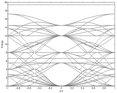
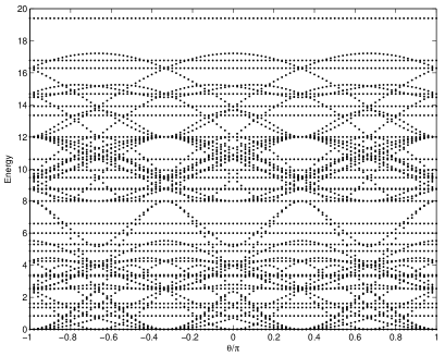
Figure 1: Spin chain with four sites. The left graph shows the energy spectrum as a function of the phase $\phi$, when $q=e^{i\phi}$ and $h=0$. The right graph shows the spectrum as a function of the phase $\theta$, when $h=e^{i\,\theta}$ and $q=0$.

Now we are ready to start examining for which values of the parameters that Reshetikhin’s condition is still satisfied in the non-holomorphic sector. By simply looking at the matrix $\mathcal{DU}$, we see that this cannot be the case when both $h$ and $q$ vanish, and also when $q=-1$, $h=1$. At a first glance, the rest of the cases seem very promising. To ensure that Reshetikhin’s condition is satisfied, we do the following. The matrix element

$$\mathcal{DU}_{(36(j_{1}-1)+6(n-1)+k_{1},36(j_{2}-1)+6(m-1)+k_{2})}$$

with $j_{1}\neq j_{2}$ and $k_{1}\neq k_{2}$ needs to vanish. It corresponds to the matrix element

$$\alpha_{j_{1}j_{2}nmk_{1}k_{2}}E_{j_{1}j_{2}}\otimes E_{nm}\otimes E_{k_{1}k_{2}}$$

Here we have chosen to rename the indices, so that barred ones correspond to odd values and non-barred correspond to even values of the original indices. The result with Mathematica is that all these terms vanish. It can be checked that if $k_{1}\neq k_{2}$, then the following holds:

$$\alpha_{jjnmk_{1}k_{2}}=-\alpha_{nmk_{1}k_{2}\tilde{j}\tilde{j}}$$

where $j$ and $\tilde{j}$ take any values. Thus, all these terms satisfy the requested form (14). We also see that for $n\neq m$ the same holds true:

$$\alpha_{jjnmkk}=-\alpha_{nmkk\tilde{j}\tilde{j}}\,,$$

again for any $j$ and $\tilde{j}$. The only thing that remains to be checked is whether the coefficients, $\alpha_{jjnnkk}$, come out the right way. To simplify our notation, we define $\tilde{\alpha}_{jnk}\equiv\alpha_{jjnnkk}$. For a consistency check we can do the case $q=e^{i\beta}$ first, which we know is integrable. In this case, the non-zero matrix elements are

$\tilde{\alpha}_{2k,2k,2k-1}$	$=-22$,		$\tilde{\alpha}_{2k-1,2k,2k}$	$=22$
$\tilde{\alpha}_{2k-1,2k-1,2k}$	$=-22$,		$\tilde{\alpha}_{2k,2k-1,2k-1}$	$=22$,
$\tilde{\alpha}_{n,2k-1,2k}$	$=-6$,		$\tilde{\alpha}_{2k,2k-1,n}$	=$6$,
$\tilde{\alpha}_{n,2k,2k-1}$	$=-6$,		$\tilde{\alpha}_{2k-1,2k,n}$	$=6$,
$\tilde{\alpha}_{n,2k,2k}$	$=16$,		$\tilde{\alpha}_{2k,2k,n}$	$=-16$,
$\tilde{\alpha}_{n,2k-1,2k-1}$	$=16$,		$\tilde{\alpha}_{2k-1,2k-1,n}$	$=-16$,

where

$n\neq 2k,2k-1$. In order to see that the above is of the requested form (14), the $\tilde{\alpha}_{j_{1},j_{2},j_{3}}$ above can be devided into a part $\tilde{\alpha}^{R}_{j_{1},j_{2},j_{3}}$ coming from the term of the form $I\otimes A$ and a part $\tilde{\alpha}^{L}_{j_{1},j_{2},j_{3}}$ coming from $A\otimes I$. Thus $\tilde{\alpha}_{j_{1},j_{2},j_{3}}=\tilde{\alpha}^{R}_{j_{1},j_{2},j_{3}}+\tilde{\alpha}^{L}_{j_{1},j_{2},j_{3}}$ with:

$\tilde{\alpha}^{R}_{l,2k-1,2k}=-6$,		$\tilde{\alpha}^{L}_{2k,2k-1,l}=6$,
$\tilde{\alpha}^{R}_{l,2k,2k-1}=-6$,		$\tilde{\alpha}^{L}_{2k-1,2k,l}=6$,
$\tilde{\alpha}^{R}_{l,2k,2k}=16$,		$\tilde{\alpha}^{L}_{2k,2k,l}=-16$,
$\tilde{\alpha}^{R}_{l,2k-1,2k-1}=16$,		$\tilde{\alpha}^{L}_{2k-1,2k-1,l}=-16$,

here $l$ takes any value

. Thus the terms are of the right form (14), as they should. Now we do the same thing for the case $q=0$ and $h=e^{i\beta}$. In this case we cannot take the integrability for granted, since we have not found any transformation relating it to the former case, as in the holomorphic sector. If we repeat the above analysis, we obtain

$\tilde{\alpha}_{2k+3,2k+4,2k}$	$=22$,		$\tilde{\alpha}_{2k+1,2k+5,2k}$	$=-22$
$\tilde{\alpha}_{2k+2,2k+1,2k+5}$	$=22$,		$\tilde{\alpha}_{2k+4,2k,2k+1}$	$=-22$,
$\tilde{\alpha}_{n_{1},2k+1,2k+5}$	$=16$,		$\tilde{\alpha}_{2k+1,2k+5,n_{2}}$	=$-16$,
$\tilde{\alpha}_{n_{1},2k+4,2k}$	$=16$,		$\tilde{\alpha}_{2k+4,2k,n_{3}}$	$=-16$,
$\tilde{\alpha}_{2k+5,2k,n_{3}}$	$=6$,		$\tilde{\alpha}_{n_{4},2k+5,2k}$	$=-6$,
$\tilde{\alpha}_{2k,2k+5,n_{2}}$	$=6$,		$\tilde{\alpha}_{n_{5},2k,2k+5}$	$=-6$,

where

$n_{1}\neq 2k+2,2k+3$, $n_{2}\neq 2k+3,2k$, $n_{3}\neq 2k+5,2k+2$, $n_{4}\neq 2k,2k+1$, $n_{5}\neq 2k+4,2k+5$. The terms above can be organized in the following way, which turns out also to be of the required form (14)

$\tilde{\alpha}^{R}_{l,2k+1,2k+5}=16$,		$\tilde{\alpha}^{L}_{2k+1,2k+5,l}=-16$,
$\tilde{\alpha}^{R}_{l,2k+4,2k}=16$,		$\tilde{\alpha}^{L}_{2k+4,2k,l}=-16$,
$\tilde{\alpha}^{R}_{2k+5,2k,l}=6$,		$\tilde{\alpha}^{L}_{l,2k+5,2k}=-6$,
$\tilde{\alpha}^{R}_{2k,2k+5,l}=6$,		$\tilde{\alpha}^{L}_{l,2k,2k+5}=-6$.

Thus

we conclude that also the $h$-deformed case with $h=e^{i\beta}$ and $q=0$ is integrable.

An interesting thing is to note that the case $q=-1$ and $h=1$ (which is equivalent to the $h\rightarrow\infty$ case) would have remained integrable, if it were not for the extra contribution of the D-term. Without the D-term contribution, the Hamiltonian turns out to be a sum of three decoupled Heisenberg spin chains. But even if the full Hamiltonian in these cases no longer fulfill Reshetikhin’s condition, we can find some subsectors where the Hamiltonian is diagonalizable. To identify these subsectors, we start by analysing just the D-term.

The D-term subsectors

We will start by looking for integrable subsectors of the D-term. We have seen that the full D-term does not satisfy the Reshetikhin’s condition, but it indeed consists of several subsectors where the Hamiltonian can immediately be diagonalised. One thing we notice at once is that there is a subsector where the eigenstates are of the form

$$|a\,b\,a\,b\,a\,b\,a\,b\rangle,\qquad a=1\,\mbox{or}\,\bar{1}\qquad b=2\,\mbox{or}\,\bar{2}$$ (17)

Acting on a state like this with the Hamiltonian simply gives

$$(m-n+L)|a\,b\,a\,b\,a\,b\,a\,b\rangle,\qquad n\in Z,\qquad m\in Z,$$ (18)

where $n$ is the number of all states of the type $|\bar{k}\,\bar{l}\rangle$ or $|k\,l\rangle$, and $m$ is the number of all states of the type $|k\,\bar{l}\rangle$ or $|\bar{k}\,l\rangle$, and $L$ is the total number of states $|a\rangle$, $|b\rangle$. We see that if we add the F-term contribution when $h\rightarrow\infty$ and also when both $q=0$ and $h=0$, these states will still be eigenstates.

Another diagonal subsector can be built up of states consisting of

$$|A\rangle=|3\rangle\otimes(|2\rangle\otimes|\bar{2}\rangle-|1\rangle\otimes|\bar{1}\rangle)\otimes|3\rangle$$ (19)

$$|B\rangle=|3\rangle\otimes(|\bar{2}\rangle\otimes|2\rangle-|\bar{1}\rangle\otimes|1\rangle)\otimes|3\rangle$$ (20)

acting with the Hamiltonian on $|A\rangle$, respectively $|B\rangle$, gives

$$H|A\rangle=4|A\rangle,\qquad H|B\rangle=4|B\rangle,\qquad\mbox{and}\qquad H\,|A\rangle\otimes|B\rangle=10|A\rangle\otimes|B\rangle$$ (21)

We can continue making this little game also when adding F-terms coming from the diagonal ones in the holomorphic sector. Here we will do it for the $q=0$ and $h=0$ case. If we make an Ansatz that this state will be diagonal,

$$|Zup\rangle=|3\rangle\otimes(\alpha\,|2\rangle\otimes|\bar{2}\rangle+\beta\,|1\rangle\otimes|\bar{1}\rangle+\gamma\,|\bar{2}\rangle\otimes|2\rangle+\delta\,|\bar{1}\rangle\otimes|1\rangle)|3\rangle$$ (22)

then it will be an eigenstate if $\gamma=\beta=0$ and $\alpha=\delta$. We will call this eigenstate $|Zip\rangle$,

$$|Zip\rangle=|3\rangle\otimes(\alpha\,|2\rangle\otimes|\bar{2}\rangle+\delta\,|\bar{1}\rangle\otimes|1\rangle)|3\rangle\,.$$ (23)

With the Hamiltonian acting on the open state $|Zip\rangle$

$$H|Zip\rangle=8|Zip\rangle$$ (24)

It will also be an eigenstate if $\gamma=-\beta$ and $\delta=-\alpha$ and $Y_{\pm}=\alpha/\beta=-2\pm\sqrt{5}$, namely

$$|Zap_{\pm}\rangle=|3\rangle\otimes(Y_{\pm}\,|2\rangle\otimes|\bar{2}\rangle+|1\rangle\otimes|\bar{1}\rangle-|\bar{2}\rangle\otimes|2\rangle-Y_{\pm}\,|\bar{1}\rangle\otimes|1\rangle)|3\rangle\,.$$ (25)

The Hamiltonian acting on the open state $|Zap\rangle$ gives

$$H|Zap_{\pm}\rangle=(10+2Y_{\pm})|Zap_{\pm}\rangle$$ (26)

From this more general eigenstates with combinations of $Zip$ and $Zap$ states can be constructed,

$$|Zip\rangle^{n_{1}}|Zap_{\pm}\rangle^{n_{2}}\ldots|Zip\rangle^{n_{45}}\,.$$ (27)

4 An integrable sector with $\mathfrak{su}_{q}(3)$ symmetry

In this section we will show the existence of an integrable three-state subsector of the full scalar field theory, with $\mathfrak{su}_{q}(3)$ symmetry, for general complex values for $q$, with $h=0$. We notice, from the interaction terms in the full Hamiltonian (3), that such a subsector exists. It consists of the states $|a\rangle$ with $a=i,\overline{i+1},i+2$, e.g. $a=1,\bar{2},3$. This subsector has two holomorphic and one anti-holomorphic field (not a conjugate of any of the two holomorphic ones). The nearest neigbour part of the Hamiltonian in this sector is

$$h_{i,i+1}=\frac{2}{|q|^{-1}+|q|}\left(\frac{|q|^{-1}+|q|}{2}\left(E_{11}\otimes E_{\bar{2}\bar{2}}+E_{\bar{2}\bar{2}}\otimes E_{11}+E_{00}\otimes E_{\bar{2}\bar{2}}+E_{\bar{2}\bar{2}}\otimes E_{00}\right)+\right.$$

$$+\left(|q|^{-1}E_{11}E_{00}+|q|\,E_{00}\otimes E_{11}\right)$$

$$\left.-\left(e^{i\beta}\,(E_{10}\otimes E_{01}+E_{1\bar{2}}\otimes E_{\bar{2}1}+E_{\bar{2}0}\otimes E_{0\bar{2}})+h.c.\right)\right)$$

The phase $\beta$ is defined by $q=|q|e^{i\beta}$. We notice in passing that when $q=1$, this becomes the ordinary Heisenberg spin-chain Hamiltonian. In [24], all integrable Hamiltonians with symmetry $U(1)^{3}$ were classified. It is easily seen that the Hamiltonian above has this symmetry. First of all, it was shown that phases can be transformed away, as they did not affect the Yang-Baxter equation. Therefore the phase $e^{i\beta}$ can be disregarded from the further analysis. We now set it equal to one, and when we later write the R-matrix for the system, we can re-insert the phases if we so desire.

This implies that we can immediately check the integrability conditions given in [24]. But first, let us introduce some notation. The Hamiltonian is written as

$$h_{i,i+1}=h_{kn}^{lm}\,E_{lk}\otimes E_{mn}.$$

The norm of the off-diagonal elements are all equal, and denoted by $r$. Then the integrability condition, which was obtained in [24] from demanding that the S-matrix satisfying the Yang-Baxter equation, reads

$$\tau_{1}\,\tau_{2}=r^{2},\qquad\sigma_{1}=\sigma_{2}=\tau_{1}+\tau_{2},$$ (28)

where

$$\tau_{1}=h_{10}^{10}-h_{00}^{00}-h_{12}^{12}+h_{02}^{02}=\frac{2|q|^{-1}}{|q|^{-1}+|q|},$$ (29)

$$\tau_{1}=h_{01}^{01}-h_{00}^{00}-h_{21}^{21}+h_{20}^{20}=\frac{2|q|}{|q|^{-1}+|q|},$$ (30)

$$\sigma_{1}=h_{10}^{10}-h_{00}^{00}-h_{11}^{11}+h_{01}^{01}=2,$$ (31)

$$\sigma_{2}=h_{20}^{20}-h_{00}^{00}-h_{22}^{22}+h_{02}^{02}=2.$$ (32)

In our case,

$$r=\frac{2}{|q|^{-1}+|q|}.$$ (33)

Thus the Hamiltonian satisfies the integrability conditions. We see that the condition on the term in front of the F-term obtained from integrability is the same as the one coming from the finiteness condition. In [24], the Hamiltonians with six off-diagonal elements were divided in three classes. We see that our Hamiltonian belongs to the same class as the Hamiltonian with $\mathfrak{su}_{q}(3)$ symmetry mentioned in [23], which came from the $A_{2}$ hyperbolic R-matrix [28]. Actually after a closer look we notice that these Hamiltonians are in fact related to each other by a term

$$\frac{|q|^{-1}-|q|}{|q|^{-1}+|q|}\left(E_{\bar{2}\bar{2}}\otimes I-I\otimes E_{\bar{2}\bar{2}}\right).$$

This term will cancel out for a periodic spin chain like the one we have, but even so we might want to find the explicit R-matrix for our Hamiltonian (4). Actually, it turns out to be very easy in this case, because we have two different types of subsectors which are related to each other in a very neat way. The first is spanned by $|1\rangle$ and $|\bar{2}\rangle$, or $|0\rangle$ and $|\bar{2}\rangle$, and the second by $|1\rangle$ and $|0\rangle$. The Hamiltonian of the latter can be written, up to a multiplicative factor $2/(|q|^{-1}+|q|)$, as

$$h_{i,i+1}=e_{i}=\pmatrix{0&0&0&0\cr 0&|q|^{-1}&-1&0\cr 0&-1&|q|&0\cr 0&0&0&0}.$$ (34)

The latter is a nice (and famous) Hamiltonian. It satisfies the Temperley-Lieb-Jones algebra

$$e_{i}e_{i+1}e_{i}=e_{i}$$ (35)

$$e_{i}e_{j}=e_{j}e_{i}\qquad;\qquad|j-i|>2$$ (36)

$$e_{i}^{2}=(|q|+|q|^{-1}).$$ (37)

which makes it possible to write the $R$-matrix for this in a very nice form [32]

$$\hat{R}=I+\frac{\sinh\,(u)}{\sinh\,(\gamma-u)}\,e_{i},\qquad|q|=e^{\gamma}.$$ (38)

This R-matrix gives the Hamiltonian (34), up to a multiplicative factor $1/(|q|-|q|^{-1})$, through the procedure (1).

Moving on to the Hamiltonian for the subsector spanned by $|1\rangle$ and $|\bar{2}\rangle$, or $|0\rangle$ and $|\bar{2}\rangle$, is:

$$h_{i,i+1}=\pmatrix{0&0&0&0\cr 0&\frac{|q|+|q|^{-1}}{2}&-1&0\cr 0&-1&\frac{|q|+|q|^{-1}}{2}&0\cr 0&0&0&0}.$$ (39)

This one has the form of the usual XXZ two-particle $R$-matrix:

$$\hat{R}(u)=\pmatrix{1&0&0&0\cr 0&b&c&0\cr 0&c&b&0\cr 0&0&0&1},\qquad b=\frac{\sinh(\gamma)}{\sinh(\gamma-u)},\qquad c=\frac{\sinh(u)}{\sinh(\gamma-u)},$$ (40)

with $|q|=e^{\gamma}$. We see that the $c$ is the same as in the other $R$-matrix (38). The derivative of $c$ taken at zero is $1/\sinh(\gamma)=1/(|q|-|q|^{-1})$, and the derivative of $b$ at zero is $\cosh(\gamma)/\sinh(\gamma)=(|q|+|q|^{-1})/(|q|-|q|^{-1})$. Thus we get the Hamiltonian (39) up to the same multiplicative factor as when we got the Hamiltonian (34) case when extracting the Hamiltonian through (1).

Matching these two R-matrices together we then have to check that the terms in the Yang-Baxter equation involving all three fields cancel each other out. We have verified that this is the case, and we get a total R-matrix for the full Hamiltonian (4)

$$\hat{R}(u)= E_{11}E_{11}+E_{\bar{2}\bar{2}}E_{\bar{2}\bar{2}}+E_{33}E_{33}+$$ (44)

$$+\frac{\sinh(\gamma)}{\sinh(\gamma-u)}\left(E_{11}E_{\bar{2}\bar{2}}+E_{\bar{2}\bar{2}}E_{11}+E_{33}E_{\bar{2}\bar{2}}+E_{\bar{2}\bar{2}}E_{33}\right)$$

$$(1+\frac{\sinh(u)\,e^{\gamma}}{\sinh(\gamma-u)})E_{11}E_{33}+(1+\frac{\sinh(u)\,e^{-\gamma}}{\sinh(\gamma-u)})E_{33}E_{11}$$

$$-\frac{\sinh(u)}{\sinh(\gamma-u)}\left(e^{i\beta}\,(E_{13}E_{31}+E_{1\bar{2}}E_{\bar{2}1}+E_{\bar{2}3}E_{3\bar{2}})+h.c.\right)$$

This R-matrix just gives rise to the same Bethe equations as the $\mathfrak{su}_{q}(3)$ invariant $A_{2}$ model when using the nested Bethe Ansatz, if $\beta$ is zero [28]. This is because the only difference between this R-matrix and the R-matrix for the $A_{2}$ model is the terms $\hat{R}_{ij}^{ij}$, $i\neq j$. These terms cancels out of the Bethe equations because

$$\frac{\hat{R}_{ij}^{ij}(u)}{\hat{R}_{ij}^{ji}(u)}=-\frac{\hat{R}_{ij}^{ij}(-u)}{\hat{R}_{ij}^{ji}(-u)}.$$

In [22] the authors studying R-matrices with phases appearing in the same way as in our R-matrix, and we can use the result given there to include the phases. After including these phases we get the following set of algebraic Bethe equations:

$$\prod_{l\neq k}^{K_{2}}\frac{\sinh((\mu_{2,k}-\mu_{2,l})-\gamma)}{\sinh((\mu_{2,k}-\mu_{2,l})+\gamma)}\prod_{j=1}^{K_{1}}\frac{\sinh((\mu_{2,k}-\mu_{1,j})+\gamma/2)}{\sinh((\mu_{2,k}-\mu_{1,j})-\gamma/2)}=e^{i(2\,n_{1}+n_{2}+n_{3})\beta}$$ (45)

$$e^{-i(n_{1}+n_{2})\beta}\left(\frac{\sinh(\mu_{1,k}+\gamma/2)}{\sinh(\mu_{1,k}-\gamma/2)}\right)^{L}=$$ (46)

$$\prod_{l\neq k}^{K_{1}}\frac{\sinh((\mu_{1,k}-\mu_{1,l})+\gamma)}{\sinh((\mu_{1,k}-\mu_{1,l})-\gamma)}\,\prod_{j=1}^{K_{2}}\frac{\sinh((\mu_{1,k}-\mu_{2,j})-\gamma/2)}{\sinh((\mu_{1,k}-\mu_{2,j})+\gamma/2)}$$ (47)

as well as the cyclicity constraint:

$$e^{i(-n_{2}+n_{3})\beta}\prod_{l}^{K_{1}}\frac{\sinh(\mu_{1,l}+\gamma/2)}{\sinh(\mu_{1,l}-\gamma/2)}=1$$ (48)

Here we have chosen a notation where by $n_{1}$ is related to $|\bar{2}\rangle$, $n_{2}$ is related to $|3\rangle$ and $n_{3}$ is related to $|1\rangle$. Also, $L=n_{1}+n_{2}+n_{3}$ and $K_{2}=n_{2}+n_{3}$.

5 The holomorphic sector

The one-loop dilatation operator for the Leigh-Strassler deformation in the holomorphic sector was given in [27] as a nearest neighbour spin chain Hamiltonian. Now we are interested in whether this spin chain Hamiltonian is integrable for any other parameter values than in the cited work. There, the authors hoped for the existence of an R-matrix which would give rise to more cases. Indeed, an elliptic R-matrix exists, the Belavin R-matrix [31], which has the right symmetry. But as we will see, unfortunately neither it, nor any other elliptic or trigonometric R-matrix, can possibly give rise to any more cases.

We start out by writing out the above mentioned spin chain Hamiltonian such that all explicit interactions are clearly visible:

$$H=\sum_{l}h_{l,l+1},$$ (49)

where

$$h_{l,l+1} = E_{i,i}\otimes E_{i+1,i+1}-qE_{i+1,i}\otimes E_{i,i+1}-q^{*}E_{i,i+1}\otimes E_{i+1,i}$$ (50)

$$+ qq^{*}E_{i+1,i+1}\otimes E_{i,i}-qh^{*}E_{i+1,i+2}\otimes E_{i,i+2}-q^{*}hE_{i+2,i+1}\otimes E_{i+2,i}$$

$$+ hE_{i+2,i}\otimes E_{i+2,i+1}+h^{*}E_{i,i+2}\otimes E_{i+1,i+2}+hh^{*}E_{i,i}\otimes E_{i,i}\,.$$

Here, the operators $E_{ij}$ are defined to act on the basis states as $E_{ij}|k\rangle=\delta_{jk}|i\rangle$. The Hamiltonian can be rewritten in a form which makes the $Z_{3}\times Z_{3}$ symmetry more apparent:

$$h_{l,l+1}=\sum_{n,m=0}^{2}\,\omega_{nm}S_{n,m}\otimes S_{2n,2m}\,.$$ (51)

The generators $S_{n,m}$ can be defined in terms of a product $S_{n,m}=e^{i2\pi nm/3}S^{n}_{1,0}S^{m}_{0,1}$ with

$$S_{1,0}=\pmatrix{0&1&0\cr 0&0&1\cr 1&0&0},\qquad S_{0,1}=\pmatrix{e^{\frac{-i2\pi}{3}}&0&0\cr 0&1&0\cr 0&0&e^{\frac{i2\pi}{3}}}.$$ (52)

The generators are related by

$$S_{n,m}S_{l,k} = e^{-i\frac{2\pi(nk-ml)}{3}}S_{n+m,k+l}\,,$$ (53)

where the indices are defined modulo three. The coefficients $\omega_{nm}$ are related to $h$ and $q$ as

$$\omega_{0,k}=\left(h\,h^{*}+q\,q^{*}\,e^{-\frac{i\,2\,\pi\,k}{3}}+e^{\frac{i\,2\,\pi\,k}{3}}\right)/3,$$ (54)

$$\omega_{1,k}=\left(-q^{*}+h\,e^{-\frac{i\,2\,\pi\,k}{3}}-q\,h^{*}\,e^{\frac{i\,2\,\pi\,k}{3}}\right)/3,$$ (55)

$$\omega_{2,k}=\left(-q+h^{*}e^{-\frac{i\,2\,\pi\,k}{3}}-q^{*}h\,e^{\frac{i\,2\,\pi\,k}{3}}\right)/3.$$ (56)

It can be easily shown that this is the most general form for a Hamiltonian with the local property $h_{i,i+1}^{2}\propto h_{i,i+1}$. The Belavin R-matrix gives rise to Hamiltonians of the form (51) mentioned above,

$$R(u)=\sum_{n,m=0}^{2}\,w_{nm}(u)S_{n,m}\otimes S_{2n,2m}\,.$$ (57)

The weights are given as

$$w_{nm}(u)=e^{\frac{-i2\pi}{3}(1-m)u}\frac{\theta_{1}(u+\gamma+\frac{n}{3}+\frac{m\tau}{3})}{\theta_{1}(\gamma+\frac{n}{3}+\frac{m\tau}{3})}\;.$$ (58)

This R-matrix is regular, which means that it is the permutation matrix when $u=0$, and the Hamiltonian can then be obtained as discussed in the section two. It also satisfies the unitarity condition, and therefore the Hamiltonian obtained from this R-matrix will automatically satisfy Reshetikhin’s condition. This condition will now be used to show that we cannot obtain any additional integrable cases for the Leigh-Strassler deformation. Reshetikhin’s condition simplifies when $h_{i,i+1}^{2}\propto h_{i,i+1}$, and takes the form

$$-2\,h_{i,i+1}h_{i+1,i+2}h_{i,i+1}+2\,h_{i+1,i+2}h_{i,i+1}h_{i+1,i+2}=I\otimes A-A\otimes I\,.$$ (59)

In Appendix (A) we show that, due to the symmetry, we will always have that if the left hand side has a term $I\otimes A$, there is also a term $-A\otimes I$. The left hand term can be written explicitly as

$$h_{i,i+1}h_{i+1,i+2}h_{i,i+1}=\sum_{l,k,\bar{l},\bar{k}=0}^{2}\,h^{L}_{l\,k\,\bar{l}\,\bar{k}}\,S_{lk}\otimes S_{\bar{l}-l,\bar{k}-k}\otimes S_{2\bar{l},2\bar{k}}$$ (60)

$$h_{i+1,i+2}h_{i,i+1}h_{i+1,i+2}=\sum_{l,k,\bar{l},\bar{k}=0}^{2}\,h^{R}_{l\,k\,\bar{l}\,\bar{k}}\,S_{lk}\otimes S_{\bar{l}-l,\bar{k}-k}\otimes S_{2\bar{l},2\bar{k}}\;,$$ (61)

where the coefficients $h^{L}_{l\,k\,\bar{l}\,\bar{k}}$ and $h^{R}_{l\,k\,\bar{l}\,\bar{k}}$ are

$$h^{L}_{l\,k\,\bar{l}\,\bar{k}}=\sum_{m,n}\,\omega_{nm}\omega_{\bar{l}\bar{k}}\omega_{l-n,k-m}\eta^{-ml+m\bar{l}-\bar{k}n+kn-\bar{k}l+\bar{l}k}$$ (62)

$$h^{R}_{l\,k\,\bar{l}\,\bar{k}}=\sum_{m,n}\,\omega_{nm}\omega_{l\,k}\omega_{\bar{l}-n,\bar{k}-m}\eta^{-m\bar{l}+m\,l-k\,n+\bar{k}n-k\,\bar{l}+l\bar{k}}$$ (63)

Now we would like to find all the solutions to the equation (59). Many of these equations are linearly dependent, so we need only a few of them. Here we will just state the result, for details see Appendix (A):

$$h=0,\qquad q=e^{i\phi},$$ (64)

$$h=e^{i\,\theta},\qquad q=0$$ (65)

$$h=\rho\,e^{i\frac{2n\pi}{3}},\qquad q=(1+\rho)\,e^{i\,\frac{2\pi m}{3}},$$ (66)

$$h=e^{i\frac{2n\pi}{3}},\qquad q=-e^{i\frac{2m\pi}{3}}$$ (67)

$$h=0,\qquad q=0$$ (68)

In conclusion, we do not find any additional integrable cases. The cases $r=0$, $\rho=0$ and also $r=1$, $\rho=1$ are a bit special, in the sense that the second charge disappears. So one might think that they are not integrable, but these are limiting cases of Hamiltonians which have an infinite amount of commuting charges, so this is not a problem. In another sense, one could think of them as trivially integrable, because they are already diagonal from the beginning and will trivially describe factorized scattering.

Now we would also like to prove that we cannot have any Hermitian Hamiltonian of the form (51) satisfying the Reshetikhin’s condition, except ones which can be related to this by a $e^{i2n\pi/3}$ site dependent shift, together with a normal change of basis to a Hamiltonian with a $U(1)^{3}$ symmetry. Therefore we will just remove the condition $h_{i}^{2}=h_{i}$. The coefficient $\omega_{ij}$ will now be written as

$$\omega_{0,k}=\left(a+b\,e^{\frac{-i\,2\,\pi\,k}{3}}+e^{\frac{i\,2\,\pi\,k}{3}}\right)/3\;,$$ (69)

$$\omega_{1,k}=\left(c+e\,e^{-\frac{i\,2\,\pi\,k}{3}}+d\,e^{\frac{i\,2\,\pi\,k}{3}}\right)/3\;,$$ (70)

$$\omega_{2,k}=\left(c+e\,e^{-\frac{i\,2\,\pi\,k}{3}}+d\,e^{\frac{i\,2\,\pi\,k}{3}}\right)/3\;.$$ (71)

The full Reshetikhin’s condition reads

$$h_{i,i+1}^{2}\,h_{i+1,i+2}-h_{i,i+1}h_{i,i+2}^{2}-h_{i+1,i+2}^{2}h_{i,i+1}+h_{i+1,i+2}h_{i,i+1}^{2}$$ (72)

$$-2\,h_{i,i+1}h_{i+1,i+2}h_{i,i+1}+2\,h_{i+1,i+2}h_{i,i+1}h_{i+1,i+2}=I\otimes A-A\otimes I$$ (73)

The new terms are as follows

$$h_{i,i+1}^{2}\,h_{i+1,i+2}=\sum_{m,n}\,\omega_{nm}\omega_{\bar{l}\bar{k}}\omega_{l-n,k-m}\eta^{ml-nk-k\bar{l}+l\bar{k}}S_{lk}\otimes S_{\bar{l}-l,\bar{k}-k}\otimes S_{2\bar{l},2\bar{k}}$$ (74)

$$h_{i,i+1}\,h_{i+1,i+2}^{2}=\sum_{m,n}\,\omega_{nm}\omega_{l\,k}\omega_{\bar{l}-n,\bar{k}-m}\eta^{m\bar{l}-n\bar{k}-k\bar{l}+l\bar{k}}S_{lk}\otimes S_{\bar{l}-l,\bar{k}-k}\otimes S_{2\bar{l},2\bar{k}}$$ (75)

$$h_{i+1,i+2}\,h_{i,i+1}^{2}=\sum_{m,n}\,\omega_{nm}\omega_{\bar{l}\bar{k}}\omega_{l-n,k-m}\eta^{ml-nk+k\bar{l}-l\bar{k}}S_{lk}\otimes S_{\bar{l}-l,\bar{k}-k}\otimes S_{2\bar{l},2\bar{k}}$$ (76)

$$h_{i+1,i+2}^{2}\,h_{i+1,i+2}=\sum_{m,n}\,\omega_{nm}\omega_{l\,k}\omega_{\bar{l}-n,\bar{k}-m}\eta^{m\bar{l}-n\bar{k}+k\bar{l}-l\bar{k}}S_{lk}\otimes S_{\bar{l}-l,\bar{k}-k}\otimes S_{2\bar{l},2\bar{k}}$$ (77)

We can also show that if we have a term of the form $I\otimes A$ there is automatically a term $-A\otimes I$. We conclude that the only solutions which are not immediately of a $U(1)^{3}$ form are the following

$$c_{r}=-\frac{d_{r}e_{r}}{d_{r}+e_{r}},\qquad b_{r}=1-d_{r}+e_{r},\qquad a_{r}=1-d_{r}-\frac{d_{r}e_{r}}{d_{r}+e_{r}},$$ (78)

where we introduced complex polar coordinates, as $a=a_{r}e^{i\phi_{a}}$ e.t.c., where we allow for $a_{r}<0$ e.t.c.. The only allowed phases of the complex parameters being multiples of $2\pi/3$. The transformation that takes the case $h=\rho\,e^{i\frac{2n\pi}{3}}$ and $q=(1+\rho)\,e^{i\,\frac{2\pi m}{3}}$ into the $q=e^{i\phi}$ case, transforms this last case into one with a Hamiltonian where the $U(1)^{3}$ symmetry is apparent.

6 Conclusion

We have used Reshetikhin’s condition to check the integrability properties for the dilatation operator for both the holomorphic and the full scalar field sector of the general Leigh-Strassler deformation to one loop. We have been able to exclude the possibility of obtaining the dilatation operator in the holomorphic sector from an R-matrix with genus one or less, for any other values of the parameters than the ones already found. In the non-holomorphic sector we find that all integrable cases, except the ones corresponding to diagonal Hamiltonians in the holomorphic sector, stay integrable. It would be interesting to understand which factors decide if integrability is preserved when going from the holomorphic to the non-holomorphic sector. Generically this is not to be the case [23]. It would be interesting to obtain the Bethe equations for the $h=e^{i\theta}$, $\theta\in\mathcal{R}$ with $q=0$ in the full scalar field sector. Maybe it could help in understanding what a dual string theory background should look like.

It is interesting to see that the simplest cases in the holomorphic sector become so much harder in the non holomorphic sector. This should be visible in the dual string theory as well. Even so, we have seen that the theory has even more simple subsectors when $q=0$ and $h=0$ with non trivial eigenvalues. It would be interesting to study these limiting cases from string theory. One way to start an exploration is to consider the string background in [13, 19] for the $q$-deformed case, but the background there seems only valid for $q$ close to one. In another article, some changes were suggested that could possibly extend the validity to arbitrary $q$ values [38].

We have found a one-loop integrable subsector to the full scalar field sector which is integrable for any complex $q$ and $h=0$ in the closed sector consisting of two holomorphic fields and one anti-holomorphic or vice versa. This differs from what is the case in the holomorphic sector, where integrability exist only for $q=e^{i\beta}$, $\beta\in\mathcal{R}$. It is interesting to note that in this last case with a $q$-dependent factor in front of the F-term, both integrability and the one-loop finiteness condition coincide.

It would be interesting to see if this integrability also exists to higher loops. First of all, it has to be proven whether the $\mathfrak{su}_{q}(2)$ sector is integrable or not to higher loops. If that is the case, it would be interesting to see if an extended version of the $\mathfrak{su}_{q}(3)$ case is integrable to higher loops. This sector will not be closed anymore, so we would need to include fermions and the appropriate group would be $\mathfrak{su}_{q}(2|3)$, in analogy with the non deformed case [39, 40]. Of course, before going to higher loops it should be verified that the integrability survives the upgrading to $\mathfrak{su}_{q}(2|3)$ to one-loop.

Another interesting question would be to look for the string Bethe equations arising from the supergravity background suggested in [41, 19, 25, 29]. The purpose would be to see if the same Bethe equations can be derived from that background, and to check if it is the correct dual background for general complex parameter $q$. It would also be interesting to look at the sigma model coming from string theory side for this integrable sector, in the same fashion as was done in the non integrable holomorphic three state sector, and compare with the coherent spin chain sigma model obtained from this spin chain.

Appendix A Technical details for section 5

Reshetikhin’s condition will now be used to show that we cannot obtain any additional integrable cases for the Leigh-Strassler deformation. Reshetikhin’s condition simplifies when $h_{i,i+1}^{2}\propto h_{i,i+1}$, and takes the form

$$-2\,h_{i,i+1}h_{i+1,i+2}h_{i,i+1}+2\,h_{i+1,i+2}h_{i,i+1}h_{i+1,i+2}=I\otimes A-A\otimes I\,.$$ (79)

We will see that, due to the symmetry, we will always have that if the left hand side has a term $I\otimes A$, there is also a term $-A\otimes I$. The left hand terms can be written explicitly as

$$h_{i,i+1}h_{i+1,i+2}h_{i,i+1}=\sum_{l,k,\bar{l},\bar{k}=0}^{2}\,h^{L}_{l\,k\,\bar{l}\,\bar{k}}\,S_{lk}\otimes S_{\bar{l}-l,\bar{k}-k}\otimes S_{2\bar{l},2\bar{k}}$$ (80)

$$h_{i+1,i+2}h_{i,i+1}h_{i+1,i+2}=\sum_{l,k,\bar{l},\bar{k}=0}^{2}\,h^{R}_{l\,k\,\bar{l}\,\bar{k}}\,S_{lk}\otimes S_{\bar{l}-l,\bar{k}-k}\otimes S_{2\bar{l},2\bar{k}}\;,$$ (81)

where the coefficients $h^{L}_{l\,k\,\bar{l}\,\bar{k}}$ and $h^{R}_{l\,k\,\bar{l}\,\bar{k}}$ are

$$h^{L}_{l\,k\,\bar{l}\,\bar{k}}=\sum_{m,n}\,\omega_{nm}\omega_{\bar{l}\bar{k}}\omega_{l-n,k-m}\eta^{-ml+m\bar{l}-\bar{k}n+kn-\bar{k}l+\bar{l}k}$$ (82)

$$h^{R}_{l\,k\,\bar{l}\,\bar{k}}=\sum_{m,n}\,\omega_{nm}\omega_{l\,k}\omega_{\bar{l}-n,\bar{k}-m}\eta^{-m\bar{l}+m\,l-k\,n+\bar{k}n-k\,\bar{l}+l\bar{k}}$$ (83)

$S_{00}$ is the identity matrix, so the $A\otimes I$ term is

$$\sum_{m,n}\,(\omega_{nm}\omega_{00}\omega_{l-n,k-m}\eta^{-ml+kn}+\omega_{nm}\omega_{l\,k}\omega_{2n,2m}\eta^{m\,l-k\,n})S_{lk}\otimes S_{2l,2k}\otimes S_{0,0}\,,$$ (84)

and the $I\otimes A$ term is

$$\sum_{m,n}\,(\omega_{nm}\omega_{\bar{l}\bar{k}}\omega_{l-n,k-m}\eta^{m\bar{l}-\bar{k}n}+\omega_{nm}\omega_{00}\omega_{\bar{l}-n,\bar{k}-m}\eta^{-m\bar{l}+\bar{k}n})S_{00}\otimes S_{\bar{l},\bar{k}}\otimes S_{2\bar{l},2\bar{k}}\,.$$ (85)

The coefficient of $S_{00}\otimes S_{lk}\otimes S_{2l,2k}$ is equal to the coefficient of $S_{lk}\otimes S_{2l,2k}\otimes S_{00}$. Now we would like to find all the solutions to the equation (59). Many of the equations are linearly dependent, so we need only a few of them. We will write the $q$ and $h$ in complex polar coordinates, as $q=-re^{i\phi}$ and $h=\rho e^{i\theta}$, where we allow for $r,\rho<0$. The equations coming from {$l,k,\bar{l},\bar{k}=1,3,2,1$} and {$l,k,\bar{l},\bar{k}=1,3,2,2$} will restrict the number of possible cases drastically. These two equations are

$$0=\frac{1}{6}\rho\,r\,(e^{i\frac{2\pi}{3}}+e^{-i\frac{2\pi}{3}}\rho^{2}+r^{2})\times$$ (86)

$$(e^{i3(\theta+\phi)}+e^{i3(\phi)}\rho+e^{i3(\theta)}r-(e^{-i3(\theta+\phi)}+e^{-i3(\phi)}\rho+e^{-i3(\theta)}r)(e^{i3(\theta+\phi)+i\frac{2\pi}{3}}))$$

$$0=\frac{1}{6}\rho\,r\,(e^{i\frac{2\pi}{3}}+e^{-i\frac{2\pi}{3}}\rho^{2}+r^{2})\times$$ (87)

$$(e^{i3(\theta+\phi)}+e^{i3(\phi)}\rho+e^{i3(\theta)}r-(e^{-i3(\theta+\phi)}+e^{-i3(\phi)}\rho+e^{-i3(\theta)}r)(e^{i3(\theta+\phi)-i\frac{2\pi}{3}}))$$

Obviously, these two equations are satisfied when either $r=0$, $\rho=0$, or $r^{2}=1$ and $\rho^{2}=1$. Now let us check for zeroes of the second parantheses. There are two possibilities. Firstly, $\theta=2\pi m/3$, $\phi=2\pi n/3$ together with $r=-1-\rho$, and secondly

$$r=-\frac{\sin 3\theta}{\sin 3(\theta-\phi)}\qquad\rho=\frac{\sin 3\phi}{\sin 3(\theta-\phi)}.$$

For the first case all equations is automatically solved. In the latter case, most of the equations will vanish, but e.g. the equation coming from {$l,k,\bar{l},\bar{k}=3,1,2,3$} takes the form

$$\frac{\left(1-e^{i\,6\phi}\right)^{2}\,\left(1-e^{i\,6\phi}\right)^{2}}{\left(e^{i6\theta}-e^{i6\phi}\right)^{4}}(e^{i4\theta}+e^{i2\phi}+e^{2i(\theta+2\phi)})\times$$ (88)

$$\left(e^{i6\theta}+e^{i2(4\,\phi+\theta)}+e^{i\frac{2\pi}{3}}(e^{i6\phi}+e^{i2(\phi+4\,\theta)})+e^{-i\frac{2\pi}{3}}(e^{i2(\phi+\theta)}+e^{i6(\phi+\theta)})\right).$$ (89)

This equation restricts one of the angles to be $n\pi/3$. Further, this implies that one of $r$ or $\rho$ is zero, and the other is one, e.g. if $\phi=\pi/3$ we have $r=0$. So these cases are not interesting.

Now we go on to investigate the case with $r^{2}=1$ and $\rho^{2}=1$. Without loss of generality, we can restrict to $r=1$ and $\rho=1$, since we still have a phase factor. The equation coming from {$l,k,\bar{l},\bar{k}=3,1,2,2$} yields the two real equations

$$\cos(2\theta-\phi)-e^{i\frac{9\phi}{2}}\cos(\theta-\frac{\phi}{2})=0$$ (90)

$$\cos(2\phi-\theta)-e^{-i\frac{9\theta}{2}}\cos(\phi-\frac{\theta}{2})=0\,,$$ (91)

and the equation coming from {$l,k,\bar{l},\bar{k}=3,1,2,1$} implies that either

$$1+2\,e^{-\frac{3\phi}{2}}\cos(-\frac{2\pi}{3}+\theta-\frac{\phi}{2})=0,$$ (92)

or

$$3+2\left(\cos(\phi+\theta)+\cos(\theta-2\phi)+\cos(\phi-2\theta)\right)=0\;.$$ (93)

Analysing these equations, we conclude that the only possibilities for the angles are $\theta=2\pi n/3$ and $\phi=2\pi n/3$.

We conclude with looking in turn at the cases $\rho=0$ and $r=0$. From the remaining equations we get the conditions

$$r^{2}-1=0\quad\mbox{or}\quad r=0\qquad\mbox{and}\qquad\rho^{2}-1=0\quad\mbox{or}\quad\rho=0\;,$$ (94)

respectively. To conclude, the following solutions exists:

$$h=0,\qquad q=e^{i\phi},$$ (95)

$$h=e^{i\,\theta},\qquad q=0$$ (96)

$$h=\rho\,e^{i\frac{2n\pi}{3}},\qquad q=(1+\rho)\,e^{i\,\frac{2\pi m}{3}},$$ (97)

$$h=e^{i\frac{2n\pi}{3}},\qquad q=-e^{i\frac{2m\pi}{3}}$$ (98)

$$h=0,\qquad q=0$$ (99)

Thus, we do not find any additional integrable cases.

Appendix B Limits of the Belavin R-matrix

It was shown a long time ago that Cherednik’s trigonometric $Z_{N}$ R-matrix can be obtained as a special limit of the Belavin R-matrix [31]. Not the full Cherednik R-matrix, but only when its parameters satisfy certain relations. This corresponds to the limit $\tau\rightarrow\infty$. We will have a look at it and see that it is only physical for the case corresponding to the ordinary Heisenberg spin chain. That Hamiltonian can also be obtained from directly taking the $\gamma\rightarrow 0$ limit on the generic Hamiltonian obtained from the original Belavin R-matrix.

To see this we first write out the elements of the R-matrix, $R=R_{km}^{ln}E_{kl}\otimes E_{mn}$ explicitly

$$R_{ll}^{ll}=a(u) = w_{01}(u)+w_{02}(u)+w_{00}(u)\,,$$

$$R_{l,l+1}^{l,l+1}=b(u) = w_{01}(u)e^{i2\pi/3}+w_{02}(u)e^{-i2\pi/3}+w_{00}(u)\,,$$

$$R_{l+1,l}^{l+1,l}=\bar{b}(u) = w_{02}(u)e^{i2\pi/3}+w_{01}(u)e^{-i2\pi/3}+w_{00}(u)\,,$$

$$R_{l,l+1}^{l+1,l}=c(u) = w_{11}(u)+w_{12}(u)+w_{10}(u)\,,$$

$$R_{l+1,l}^{l,l+1}=\bar{c}(u) = w_{21}(u)+w_{22}(u)+w_{20}(u)\,,$$ (100)

$$R^{l,l-1}_{l+1,l+1}=d(u) = w_{11}(u)e^{i2\pi/3}+w_{12}(u)e^{-i2\pi/3}+w_{10}(u)\,,$$

$$R_{l,l-1}^{l+1,l+1}=\bar{d}(u) = w_{21}(u)e^{i2\pi/3}+w_{22}(u)e^{-i2\pi/3}+w_{20}(u)\,,$$

$$R^{l-1,l-1}_{l,l+1}=e(u) = w_{12}(u)e^{i2\pi/3}+w_{11}(u)e^{-i2\pi/3}+w_{10}(u)\,,$$

$$R^{l,l+1}_{l-1,l-1}=\bar{e}(u) = w_{22}(u)e^{i2\pi/3}+w_{21}(u)e^{-i2\pi/3}+w_{20}(u)\,,$$

where

$$w_{mn}=e^{\frac{i2\pi\,m\,u}{3}}\frac{\theta_{1}(u+\gamma+\frac{n}{3}+\frac{m\tau}{3})}{\theta_{1}(\gamma+\frac{n}{3}+\frac{m\tau}{3})}$$ (101)

The Hamiltonian is obtained as in (1), expressed in terms of the derivatives of the $\omega_{ij}$

$$w_{mn}^{\prime}=\frac{i2\pi\,m}{3}+\frac{\theta_{1}^{\prime}(\gamma+\frac{n}{3}+\frac{m\tau}{3})}{\theta_{1}(\gamma+\frac{n}{3}+\frac{m\tau}{3})}$$ (102)

Here we see directly that the limiting case $\gamma\rightarrow 0$ corresponds to a Heisenberg spin chain, due to the fact that the $w_{00}^{\prime}$ term blows up, leaving the Hamiltonian with just the pieces containing that term. Before we proceed to show how the Belavin R-matrix changes shape into Cherednik’s R-matrix, we will discuss the effect of the $Z_{3}\times Z_{3}$ symmetries.

The solution is invariant under any shift $w_{mn}\rightarrow w_{m+k_{1},n+k_{2}}$. These shifts can be generated from modular transformations of the above solution, taking combinations of $\tau\rightarrow-1/\tau$ and $\tau\rightarrow\tau+1$. This is shown below. The different transformations taking the $h=0$ case to the $q=0$ case correspond to shifting $w_{mn}\rightarrow w_{m+2,n}$, and $w_{mn}\rightarrow w_{nm}$ corresponds to yet another of the transformations mentioned in [27]. The modular transformation of the theta function is

$$\theta_{1}\left(v/\tau|-1/\tau\right)=\frac{1}{i}\sqrt{\frac{\tau}{i}}e^{i\pi v^{2}/\tau}\theta_{1}(v|\tau)$$ (103)

Using this we can rewrite $w_{mn}$ as

$$w_{mn}=-\frac{1}{\tau}e^{(\frac{i\pi\,m\,u}{3})}e^{-i2\pi(u^{2}+2u(\gamma+\frac{n}{3}+\frac{m\tau}{3}))/\tau}\frac{\theta_{1}(u/\tau+\gamma/\tau+\frac{n}{3\tau}+\frac{m}{3}|-1/\tau)}{\theta_{1}(\gamma/\tau+\frac{n}{3\tau}+\frac{m}{3}|-1/\tau)}$$ (104)

$$=-e^{-i2\pi(u^{2}+2u\gamma)/\tau}\frac{1}{\tau}e^{(\frac{-i\pi\,n\,u/\tau}{3})}\frac{\theta_{1}(u/\tau+\gamma/\tau+\frac{n}{3\tau}+\frac{m}{3}|-1/\tau)}{\theta_{1}(\gamma/\tau+\frac{n}{3\tau}+\frac{m}{3}|-1/\tau)}$$ (105)

The first factor is an overall factor independent of $n$ and $m$, so it has no physical implications for the Hamiltonian and can be normalized away. If we now define $\hat{\tau}=-1/\tau$, $\hat{u}=-u/\tau$, $\hat{\gamma}=-\gamma/\tau$, the above expression takes the shape

$$w_{mn}\propto\frac{1}{\tau}e^{(\frac{i\pi\,n\,\hat{u}}{3})}\frac{\theta_{1}(-\hat{u}-\hat{\gamma}-\frac{n\hat{\tau}}{3}+\frac{m}{3}|\hat{\tau})}{\theta_{1}(-\hat{\gamma}-\frac{n\hat{\tau}}{3}+\frac{m}{3}|\hat{\tau})}.$$ (106)

We therefore conclude that the shift $\tau\rightarrow-1/\tau$ corresponds to $\omega_{nm}\rightarrow\omega_{2m,n}$. The modular shift, $\tau\rightarrow\tau+1$, does not alter $\theta_{1}(x|\tau+1)\propto\theta_{1}(x|\tau)$. This means that it corresponds to an effective transformation $w_{mn}\rightarrow w_{m,n+1}$. All changes of basis in [27] correspond to linear combinations of these types of modular transformations. E.g. $w_{mn}\rightarrow w_{m+2,n}$ corresponds to the three consecutive transformations $\tau\rightarrow-1/\tau$, $\tau\rightarrow\tau+1$, $\tau\rightarrow-1/\tau$, or equivalently $\tau\rightarrow\tau/(1-\tau)$.

In this limit we have

$$\frac{\theta_{1}(u+\gamma+\frac{n}{3})}{\theta_{1}(\pi\gamma+\frac{n\pi}{3})}\rightarrow\frac{\sin(\pi u+\pi\gamma+\frac{n\pi}{3})}{\sin(\gamma+\frac{n}{3})}$$ (107)

and

$$\frac{\theta_{1}(u+\gamma+\frac{n}{3}\pm\frac{\tau}{6})}{\theta_{1}(\pi\gamma+\frac{n\pi}{3}\pm\frac{\tau}{6})}\rightarrow e^{\mp\pi u}$$ (108)

This is based on the assumption that $\gamma$ is real (taking the limit with a non-zero imaginary part gives a diagonal matrix). In this limit, the elements become

$$a(u) = \sin\pi u\,\cot\,3\pi\gamma+\cos\pi u\,,$$

$$b(u) = \sin\pi u\frac{e^{i\pi\gamma}}{\sin 3\pi\gamma}\,,$$

$$\bar{b}(u) = \sin\pi u\frac{e^{i\pi\gamma}}{\sin 3\pi\gamma}$$

$$c(u) = e^{\frac{i2\pi u}{3}}e^{-i\pi u}\,,$$

$$\bar{c}(u) = e^{\frac{-i2\pi u}{3}}e^{i\pi u}\,,$$ (109)

$$d(u) = 0\,,$$

$$\bar{d}(u) = 0\,,$$

$$e(u) = 0\,,$$

$$\bar{e}(u) = 0\,,\,.$$

We can rewrite things a little bit (redefining $iu\pi$ to $u$ and $i\pi\gamma$ to $\gamma$ and omitting an overall factor)

$$a(u) = 1\,,$$

$$b(u) = \frac{\sinh u}{\sinh(u+3\gamma)}e^{\gamma}\,,$$

$$\bar{b}(u) = \frac{\sinh u}{\sinh(u+3\gamma)}e^{-\gamma}\,,$$

$$c(u) = e^{\frac{u}{3}}\frac{\sinh\gamma}{\sinh(u+\gamma)}\,,$$

$$\bar{c}(u) = e^{\frac{-u}{3}}\frac{\sinh\gamma}{\sinh(u+\gamma)}\,.$$ (110)

The difference now between the R-matrix above and Cherednik’s R-matrix is that in the latter the exponentials in $b$ and $\bar{b}$ can be arbitrary, $e^{-g(\gamma)}$ and $e^{g(\gamma)}$ with $g$ any function. The restriction of the function to be $g(\gamma)=\gamma$ makes the Hamiltonian obtained from the R-matrix only Hermitian in the limiting case $\gamma\rightarrow 0$. Either the limit $\gamma\rightarrow 0$ can be taken before extracting the Hamiltonian, but then we also need to take the limit $u$ goes to zero, or the limit can be taken after the Hamiltonian has been extracted. The first way will result in the XXX R-matrix. But both methods will in the end result in the same Heisenberg spin chain Hamiltonian. Using the modular transformation of the original Belavin R-matrix, we can obtain the cases listed below:

$h=0$,	$q=e^{i2\,n\pi/3}$,	$\tau\rightarrow i\infty+n$
$h=e^{i\,2\,n\pi/3}$,	$q=0$,	$(\tau+n)/(1-\tau-n)\rightarrow i\infty$

References

• [1] J. M. Maldacena, The large N limit of superconformal field theories and supergravity, Adv. Theor. Math. Phys. 2 (1998) 231–252, [hep-th/9711200].
• [2] S. S. Gubser, I. R. Klebanov, and A. M. Polyakov, Gauge theory correlators from non-critical string theory, Phys. Lett. B428 (1998) 105–114, [hep-th/9802109].
• [3] E. Witten, Anti-de Sitter space and holography, Adv. Theor. Math. Phys. 2 (1998) 253–291, [hep-th/9802150].
• [4] J. A. Minahan and K. Zarembo, The Bethe-ansatz for $\mathcal{N}=\mathord{}$4 super Yang-Mills, JHEP 0303 (2003) 013, [hep-th/0212208].
• [5] N. Beisert and M. Staudacher, The N = 4 SYM integrable super spin chain, Nucl. Phys. B670 (2003) 439–463, [hep-th/0307042].
• [6] N. Beisert, C. Kristjansen, and M. Staudacher, The dilatation operator of $\mathcal{N}=\mathord{}$4 conformal super yang-mills theory, Nucl. Phys. B664 (2003) 131–184, [hep-th/0303060].
• [7] N. Beisert, B. Eden, and M. Staudacher, Transcendentality and crossing, hep-th/0610251.
• [8] N. Beisert, R. Hernandez, and E. Lopez, A crossing-symmetric phase for ads(5) x s**5 strings, JHEP 11 (2006) 070, [hep-th/0609044].
• [9] R. G. Leigh and M. J. Strassler, Exactly marginal operators and duality in four-dimensional n=1 supersymmetric gauge theory, Nucl. Phys. B447 (1995) 95–136, [hep-th/9503121].
• [10] S. Ananth, S. Kovacs, and H. Shimada, Proof of all-order finiteness for planar beta-deformed yang-mills, JHEP 01 (2007) 046, [hep-th/0609149].
• [11] G. C. Rossi, E. Sokatchev, and Y. S. Stanev, On the all-order perturbative finiteness of the deformed n = 4 sym theory, Nucl. Phys. B754 (2006) 329–350, [hep-th/0606284].
• [12] F. Elmetti, A. Mauri, S. Penati, and A. Santambrogio, Conformal invariance of the planar beta-deformed n = 4 sym theory requires beta real, JHEP 01 (2007) 026, [hep-th/0606125].
• [13] O. Lunin and J. Maldacena, Deforming field theories with u(1) x u(1) global symmetry and their gravity duals, JHEP 05 (2005) 033, [hep-th/0502086].
• [14] S. Frolov, Lax pair for strings in Lunin-Maldacena background, hep-th/0503201.
• [15] O. Aharony, B. Kol, and S. Yankielowicz, On exactly marginal deformations of n = 4 sym and type iib supergravity on ads(5) x s**5, JHEP 06 (2002) 039, [hep-th/0205090].
• [16] A. Fayyazuddin and S. Mukhopadhyay, Marginal perturbations of n = 4 yang-mills as deformations of ads(5) x s(5), hep-th/0204056.
• [17] M. Kulaxizi, Marginal deformations of n = 4 sym and open vs. closed string parameters, hep-th/0612160.
• [18] V. Niarchos and N. Prezas, Bmn operators for n = 1 superconformal yang-mills theories and associated string backgrounds, JHEP 06 (2003) 015, [hep-th/0212111].
• [19] S. A. Frolov, R. Roiban, and A. A. Tseytlin, Gauge - string duality for superconformal deformations of $\mathcal{N}=\mathord{}$4 super Yang-Mills theory, hep-th/0503192.
• [20] S. A. Frolov, R. Roiban, and A. A. Tseytlin, Gauge-string duality for (non)supersymmetric deformations of N = 4 super Yang-Mills theory, JHEP 07 (2005) 045, [hep-th/0507021].
• [21] S. M. Kuzenko and A. A. Tseytlin, Effective action of beta-deformed n = 4 sym theory and ads/cft, hep-th/0508098.
• [22] N. Beisert and R. Roiban, Beauty and the twist: The Bethe ansatz for twisted N = 4 SYM, JHEP 08 (2005) 039, [hep-th/0505187].
• [23] D. Berenstein and S. A. Cherkis, Deformations of N = 4 SYM and integrable spin chain models, Nucl. Phys. B702 (2004) 49–85, [hep-th/0405215].
• [24] L. Freyhult, C. Kristjansen, and T. Månsson, Integrable spin chains with $U(1)^{3}$ symmetry and generalized Lunin-Maldacena backgrounds, hep-th/0510221.
• [25] L. F. Alday, G. Arutyunov, and S. Frolov, Green-schwarz strings in tst-transformed backgrounds, JHEP 06 (2006) 018, [hep-th/0512253].
• [26] R. Roiban, On spin chains and field theories, JHEP 09 (2004) 023, [hep-th/0312218].
• [27] D. Bundzik and T. Månsson, The general leigh-strassler deformation and integrability, JHEP 01 (2006) 116, [hep-th/0512093].
• [28] H. J. De Vega, Yang-baxter algebras, integrable theories and quantum groups, Int. J. Mod. Phys. A4 (1989) 2371–2463.
• [29] T. McLoughlin and I. Swanson, Integrable twists in ads/cft, JHEP 08 (2006) 084, [hep-th/0605018].
• [30] N. Beisert and T. Klose, Long-range gl(n) integrable spin chains and plane-wave matrix theory, J. Stat. Mech. 0607 (2006) P006, [hep-th/0510124].
• [31] A. A. Belavin, Dynamical symmetry of integrable quantum systems, Nucl. Phys. B180 (1981) 189–200.
• [32] C. Gomez, G. Sierra, and M. Ruiz-Altaba, Quantum groups in two-dimensional physics, . Cambridge, UK: Univ. Pr. (1996) 457 p.
• [33] M. G. Tetelman Sov.Phys. JETP 55(2) (1982) 306–310.
• [34] K. Madhu and S. Govindarajan, Chiral primaries in the leigh-strassler deformed n = 4 sym: A perturbative study, hep-th/0703020.
• [35] D. Z. Freedman and U. Gursoy, Comments on the beta-deformed n = 4 sym theory, JHEP 11 (2005) 042, [hep-th/0506128].
• [36] A. Parkes and P. C. West, Finiteness in rigid supersymmetric theories, Phys. Lett. B138 (1984) 99.
• [37] D. R. T. Jones and L. Mezincescu, The chiral anomaly and a class of two loop finite supersymmetric gauge theories, Phys. Lett. B138 (1984) 293.
• [38] C.-S. Chu and V. V. Khoze, String theory dual of the beta-deformed gauge theory, hep-th/0603207.
• [39] N. Beisert, The su(2—3) dynamic spin chain, Nucl. Phys. B682 (2004) 487–520, [hep-th/0310252].
• [40] N. Beisert and M. Staudacher, Long-range psu(2,2—4) bethe ansaetze for gauge theory and strings, Nucl. Phys. B727 (2005) 1–62, [hep-th/0504190].
• [41] G. Arutyunov, S. Frolov, and M. Staudacher, Bethe ansatz for quantum strings, JHEP 10 (2004) 016, [hep-th/0406256].